Symmetries and similarities of the zero-pressure-gradient turbulent boundary layer

Abstract

The symmetries and similarities of the zero-pressure-gradient turbulent boundary layer (ZPGTBL) are investigated to derive the full set of similarity variables, to derive the similarity equations, and to obtain a higher-order approximate solution of the mean velocity profile. Previous analyses have not resulted in all the similarity variables. We perform a symmetry analysis of the equations for ZPGTBL using Lie dilation groups, and obtain local, leading-order symmetries of the equations. The full set of similarity variables were obtained in terms of the boundary layer parameters. The friction velocity was shown to be the outer-layer velocity scale. The downstream evolutions of the boundary thickness and the friction velocity are obtained analytically. The dependent similarity variables are written as asymptotic expansions.By asymptotically matching the expansions, an approximate similarity solution up to the third order in the overlapping layer are obtained. These results are obtained from first principles without any major assumptions and a turbulence model. The similarities and differences between ZPGTBL and turbulent channel flows in terms of the similarity equations, the gauge functions and the approximate solutions are discussed. In particular, the leading-order expansions are identical for ZPGTBL and channel flows, supporting the notion of universality of the near-wall layer. In addition, the logarithmic frictionlaw for ZPGTBL is accurate to all orders while it is only accurate at the leading order in channel flows. The results will help further understand ZPGTBL and the issue of universality of the near-wall layer in wall-bounded turbulent flows.

1 Introduction

The zero-pressure-gradient turbulent boundary layer (ZPGTBL) is the most fundamental of turbulent boundary layers, and has been studied extensively (e.g., Klebanoff 1954; Schlichting 1956; Clauser 1956; Monin & Yaglom 1971; Sreenivasan 1989; Pope 2000; McKeon & Sreenivasan 2007; Nagib et al. 2007; Marusic et al. 2010; Smits et al. 2011). The flow consists of two layers with different scaling. The inner layer has viscous scaling and the mean velocity follows the law of the wall, and is considered universal (Prandtl 1925). The outer layer does not explicitly depend on the viscosity and the mean velocity obeys the velocity defect law (von Kármán 1930). There is a matching sublayer between the outer and inner layers where the mean velocity is generally considered to follow the log law (von Kármán 1930).

The most important fundamental understanding of a boundary layer is its similarity equations and similarity solution. The zero-pressure-gradient laminar boundary layer (the Blasius boundary layer, Blasius 1908) has the well-known similarity solution. By expressing the variables in the partial differential equations for the boundary layer in terms of the similarity variables, the equations were reduced to an ordinary differential equation, the solution of which is the similarity solution. The downstream evolutions of the boundary layer thickness and the surface stress were obtained analytically. By contrast, there has not been a similarly successful development for ZPGTBL to date, despite of the extensive past research devoted to the topic. Tennekes & Lumley (1972) were the first to obtain the leading-order mean momentum similarity equation and to use it to predict the log law. However, the boundary layer thickness $\Delta$ was defined by Clauser (1956) using an integral quantity, rather than the boundary layer parameters. In addition, its downstream evolution as well as that of the friction velocity was not predicted. With this definition of $\Delta$, the non-dimensional outer layer wall-normal coordinate, the independent similarity variable, was not fully defined, in contrast to the Blasius boundary layer, making it difficult to derive the higher-order similarity equations and to analyse the similarities. Oberlack & Khujadze (2006) performed a Lie group analysis of the two-point correlation and found a linear growth of $\Delta$. Monkewitz et al. (2007) used the same definition of the boundary layer thickness and derived an expression for the downstream evolution of the momentum thickness, which depends on the shape factor $H$, while no expression for $\Delta$ was provided. They also fitted experimental data to asymptotic expansions with the gauge functions depending on the friction Reynolds number. George & Castillo (1997) used the Reynolds-averaged boundary layer equations without the viscous terms to obtain a similarity solution. However, as will be shown in the present work, by eliminating the viscous stress terms alone, the equations do not have a similarity solution as a function of the local wall-normal coordinate.

In the meantime, much progress in understanding ZPGTBL has come from experiments. Coles (1956) proposed the wake function empirically based on experimental data, which is the departure from the log law in the outer layer. The combination of the two is proposed as the outer layer similarity profile. Much of the later work on the outer layer similarities has been based on the wake function, e.g., Perry et al. (1994), Nagib et al. (2007), McKeon & Morrison (2007), Marusic et al. (2015) and Vallikivi et al. (2015). Nevertheless, the wake function lacks an analytic origin. To gain a comprehensive understanding of the similarities of ZPGTBL, in the present work we will perform a symmetry analysis of the Reynolds-averaged boundary layer equations to derive analytically the full set of similarity variables, the evolution of the boundary layer thickness, the evolution of the friction velocity and the ordinary differential equations describing the similarity solution. We will then employ the method of matched asymptotic expansions obtain a higher-order approximate solution. To our best knowledge, this is the first time such an analysis has been carried out.

Parallel to the research on ZPGTBL, there also have been much effort to investigate turbulent channel and pipe flows, which are amenable to more rigorous asymptotic analysis (e.g., Millikan 1938; Afzal 1976), including higher-order corrections to the log law. The near-wall, “constant stress” layer in ZPGTBL is commonly believed to have much in common with channel flows, i.e., the near-wall layers in these wall flows are believed to be universal, with the log law as the leading-order velocity profile. There is also evidence against universality (e.g., McKeon & Morrison 2007; Nagib et al. 2007; Marusic et al. 2015). However, there has been essentially no theoretical analysis on the similarities and differences regarding the Reynolds number dependence between these flows, e.g., no higher-order asymptotic expansions for ZPGTBL to be compared to those for the channel flows. The present work will help shed some light on the important issue of the universality of the near-wall layers.

There have also been arguments questioning the inner-layer similarity among these flows. George & Castillo (1997) claimed that the mean advection terms in the momentum equation for ZPGTBL fundamentally changes the scaling of the outer layer mean velocity profile. They argued that the velocity defect scales with the free-stream velocity $U_{e}$ rather than the friction velocity $u_{*}$. This scaling also leads to a power-law velocity profile in the overlapping layer, which is not universal, with Reynolds number dependent exponent and coefficients. On the other hand, Jones et al. (2008) argued that both $U_{e}$ and $u_{*}$ are valid scaling candidates. In the present work we show that same as in channel and pipe flows, the friction velocity is the correct scale for the velocity defect in ZPGTBL.

The rest of the paper is organized as follows. In Section 2 we perform a symmetry analysis using Lie dilation groups and obtain the full set of similarity variables. We then derive the similarity equations as singular perturbation equations, obtain an approximate solution as asymptotic expansions and make some comparisons with measurements in Section 3, followed by Discussions and Conclusions.

2 Symmetry analysis

The Naiver-Stokes equations have a number of symmetries. One of them is that the equations are invariant under a one-parameter Lie dilation group (e.g., Bluman & Kumei 1989, Frisch 1995, Cantwell 2002), which is closely related to the scaling properties and the similarity of the solution. Since invariance of the equations under the group transformation requires a constant Reynolds number, full similarity of the solution is possible only when the Reynolds number is fixed. However, it has long been recognized that the energy-containing and flux-carrying statistics in turbulent flows at high Reynolds numbers are approximately Reynolds number invariant. The leading-order flow behaviors, including similarity properties, are approximately independent of the Reynolds number. This approximate Reynolds number invariance is associated with spontaneous breaking of symmetries of the Navier-Stokes equations from laminar to turbulent flows as the Reynolds number increases. Therefore, while the symmetries of laminar flows are exact, the symmetries of turbulent flows are only approximate. The concept of spontaneous symmetry breaking and approximate symmetry first emerged in condensed matter physics and later were key to predicting certain non-zero mass particles in Yang-Mills gauge fields (Higgs 1964, 2014; Castellani 2003). As we will show in the following, the symmetries of ZPGTBL also can only be at the leading order and be approximate. In the present work, we seek the leading-order symmetries and similarity properties and determine the higher-order corrections to account for any Reynolds-number dependence.

We use Lie dilation groups to analyse the symmetries of the Reynolds-averaged boundary layer equations. Similar to the Navier-Stokes equations, the boundary layer equations also have certain group transformation properties. Once found, the group can be used to determine the similarity variables of the equations. Then using the similarity variables, the partial differential boundary layer equations can be reduced to ordinary differential equations, whose solution is the similarity solution. For ZPGTBL, the equations are the mean momentum equation and the Reynolds stress budget (or the shear-stress budget and the turbulent kinetic budget for our analysis). We need to identify the Lie dilation group under which all three in this set of equations are invariant.

We now analyse the Lie dilation group of the equations. The Reynolds-averaged momentum equation for ZPGTBL can be written in a form similar to that given by Tennekes & Lumley (1972)

$$U\frac{\partial U}{\partial x}+V\frac{\partial U}{\partial y}=-\frac{\partial{\overline{uv}}}{\partial{y}}-\frac{\partial}{\partial x}(\overline{u^{2}}-\overline{v^{2}})+\nu\frac{\partial^{2}U}{\partial y^{2}},$$ (1)

where $U$, $V$, $\overline{uv}$, $\overline{u^{2}}$, $\overline{v^{2}}$, and $\nu$ are the streamwise and normal mean velocity components, the Reynolds shear stress, the Reynolds normal stress components and the kinematic viscosity, respectively. The finite form of the dilation group is

$$\begin{split}&\tilde{x}=e^{a}x,\ \tilde{y}=e^{b}y,\ \tilde{U}=U,\ \tilde{U}-U_{e}=e^{g}(U-U_{e}),\ \partial\tilde{U}=e^{g}\partial U,\ \tilde{V}=e^{c}V,\\ &\widetilde{\overline{uv}}=e^{d}\overline{uv},\ \widetilde{\overline{u^{2}}}=e^{d_{1}}\overline{u^{2}},\ \widetilde{\overline{v^{2}}}=e^{d_{1}}\overline{v^{2}}.\end{split}$$ (2)

where $a$, $b$ etc., are the group parameters. Note that the mean velocity can dilate differently than statistics of the velocity fluctuations, which has been pointed out by She et al. (2017) based on the argument of random dilation groups. In the context of ZPGTBL, dilation can be thought of as rescaling of the physical variables for the given free-stream velocity $U_{e}$ and $\nu$. The streamwise velocity $U$ in this problem cannot dilate because the free-stream velocity, once specified, is fixed. However, the velocity defect and the velocity differential $\partial U$ can dilate (e.g, dilate along with $u_{*}$ and $y$). We will examine the possibilities that $U-U_{e}$ and $\partial U$ do and do not dilate. Here we first examine the symmetry if they not dilate. Substitute 2 into 1 and drop the tildes in the equations for convenience hereafter, we have

$$e^{-a}U\frac{\partial U}{\partial x}+e^{c-b}V\frac{\partial U}{\partial y}=-e^{d-b}\frac{\partial{\overline{uv}}}{\partial{y}}-e^{d_{1}-a}\frac{\partial}{\partial x}(\overline{u^{2}}-\overline{v^{2}})+e^{-2b}\nu\frac{\partial^{2}U}{\partial y^{2}}.$$ (3)

For the equation to be invariant under the dilation group, the exponents for each term must be equal:

$$-a=c-b=d-b=d_{1}-a=-2b.$$ (4)

Therefore

$$a=2b,\ \ c=-b,\ \ d=-b,\ \ d_{1}=0.$$ (5)

Thus 1 with the boundary condition ($U=U_{e}$ for $y\rightarrow\infty$) is invariant under a one-parameter dilation group,

$$\tilde{x}=e^{2b}x,\ \tilde{y}=e^{b}y,\ \tilde{U}=U,\ \partial\tilde{U}=\partial U,\ \tilde{V}=e^{-b}V,\ \widetilde{\overline{uv}}=e^{-b}\overline{uv}.\ \widetilde{\overline{u^{2}}}=\overline{u^{2}},\ \widetilde{\overline{v^{2}}}=\overline{v^{2}},$$ (6)

A one-parameter dilation group fully determines the scaling of the variables in the problem and can be used to identify the similarity variables. The group specified by 5 is essentially the same as that for the zero-pressure-gradient laminar (Blasius) boundary layer (Cantwell 2002). It ($a=2b$) indicates a growth rate for the boundary layer thickness $\delta\sim x^{\frac{1}{2}}$, the same as the Blasius boundary layer, but is inconsistent with that of the turbulent boundary layer. We further consider the shear-stress budget,

$$U\frac{\partial\overline{uv}}{\partial x}+V\frac{\partial\overline{uv}}{\partial y}=-\overline{u\frac{\partial p}{\partial y}+v\frac{\partial p}{\partial x}}-\overline{v^{2}}\frac{\partial U}{\partial y}-\frac{\partial\overline{uv^{2}}}{\partial y}+\nu\frac{\partial^{2}\overline{uv}}{\partial y^{2}}-\epsilon_{uv},$$ (7)

where $\epsilon_{uv}$ is the dissipation rate, which is generally negligible. For this equation to be invariant, the exponents for the terms on the l.h.s and the second term on the r.h.s. must satisfy

$$d-a=c+d-b=d_{1}-b,$$ (8)

which leads to $d=a-b$, inconsistent with 5. Therefore, there is no dilation group under which both equations 1 and 7 are invariant. Consequently, there is no full similarity solution for which the velocity defect scales as the $U_{e}$.

We now examine the symmetry if the velocity defect and the velocity differential dilate as

$$\tilde{U}-U_{e}=e^{g}(U-U_{e}),\ \partial\tilde{U}=e^{g}\partial U,$$ (9)

The streamwise mean advection term then can be written as

$$U\frac{\partial U}{\partial x}=U_{e}\frac{\partial U}{\partial x}+(U-U_{e})\frac{\partial U}{\partial x}.$$ (10)

The exponents must satisfy

$$g-a=2g-a,$$ (11)

resulting in $g=0$, the velocity defect cannot dilate. Therefore, as in the case of the (full) Navier-Stokes equations for a general turbulent flow, there are no exact symmetries for the full ZPGTBL equations. Only approximate symmetries are possible. In seeking the approximate symmetries, we recognise that viscous effects are negligible in the outer layer whereas they play a leading-order role in the inner layer, indicating that the approximate symmetries are not global, but local. In the following we analyse the symmetries of the outer and inner layers separately.

2.1 Outer layer symmetry

For the outer layer, the leading-order symmetries or the symmetries of the leading-order equations can be obtained by dropping the Reynolds-number-dependent terms. These symmetries similar to the approximate symmetries of the Navier-Stokes equations previously investigated (e.g., Grebenev & Oberlack 2007). We first drop the viscous term in the mean momentum equation, which is explicitly Reynolds-number dependent and is a higher-order term. We note that as shown above, due to the (full) advection term (10) $U-U_{e}$ and $\partial U$ do not dilate. For the momentum equation to be invariant under the dilation group, the exponents must satisfy,

$$-a=c-b=d-b=d_{1}-a.$$ (12)

Therefore

$$c=b-a,\ \ d=b-a,\ \ d_{1}=0.$$ (13)

The mean momentum equation is therefore invariant under the two-parameter dilation group

$$\tilde{x}=e^{a}x,\ \tilde{y}=e^{b}x,\ \tilde{U}=U,\ \partial\tilde{U}=\partial U,\ \tilde{V}=e^{b-a}V,\ \widetilde{\overline{uv}}=e^{b-a}\overline{uv},\ \widetilde{\overline{u^{2}}}=\overline{u^{2}},\ \widetilde{\overline{v^{2}}}=\overline{v^{2}},$$ (14)

which does not fully determine the scaling of the variables. To determine the scaling we need to identify a one-parameter group by relating the parameters $a$ and $b$. To do so we further consider the shear-stress budget with the viscous terms dropped. For this equation to be invariant, the exponents must satisfy

$$b-2a=2b-2a-b=-b.$$ (15)

Therefore

$$a=b,$$ (16)

resulting in a one-parameter dilation group. However, this group indicates that the Reynolds shear stress does not dilate, i.e., it is a constant, and that $\delta$ grows linearly, inconsistent with the known behaviours of the turbulent boundary layer. Therefore, dropping the explicitly Reynolds-number-dependent viscous terms alone, as done by George & Castillo (1997), does not lead to the correct local symmetries. The reason is that there are other higher-order terms in the equations that do not contain the viscosity, but are implicitly Reynolds-number dependent. They also need to be identified and dropped in order to obtain the leading-order outer-layer symmetries and the leading-order outer similarity solution.

To identify the higher-order terms, we perform an order of magnitude analysis of the equations. Again we first consider the scaling choice $U-U_{e}\sim U_{e}$. With this choice, the shear production of the TKE scales as $-\overline{uv}(\partial U/\partial y)\sim u_{*}^{2}U_{e}/\delta$. Since it is the only production term, the TKE scales as $k\sim U_{e}^{2}$. The velocity variances scale the same way. The dissipation rate would scale as $k^{3/2}/\delta\sim U_{e}^{3}/\delta$ (Taylor 1935), asymptotically larger than the production rate, indicating that the scaling choice $U-U_{e}\sim U_{e}$ is inconsistent with the scaling of the dissipation rate. Therefore, the velocity defect cannot scale as $U_{e}$.

With $U_{e}$ ruled out, the only scaling choice for the velocity defect is $U-U_{e}\sim u_{*}$, as there are no other velocity scales in the problem. Again, to obtain the one-parameter dilation group that is consistent with the leading-order local symmetries of the outer layer, additional terms that do not contain $\nu$, but still depend on the Reynolds number must be identified and dropped. We perform an order of magnitude analysis of the mean momentum equation and the shear stress budget to identify the leading-order terms, which are Reynolds-number independent. The orders of magnitude of the terms in the mean momentum equation are

$$\begin{split}&U_{e}\frac{\partial U}{\partial x}+(U-U_{e})\frac{\partial U}{\partial x}\hskip 5.69046pt+\hskip 7.11317ptV\frac{\partial U}{\partial y}\hskip 7.11317pt=\hskip 7.11317pt-\frac{\partial\overline{uv}}{\partial y}-\frac{\partial(\overline{u^{2}}-\overline{v^{2}})}{\partial x}+\nu\frac{\partial^{2}U}{\partial y^{2}}\\ &\ U_{e}\frac{u_{*}}{L}\hskip 22.76228pt\frac{u_{*}{{}^{2}}}{L}\hskip 42.67912ptV\frac{u_{*}}{\delta}=\frac{u_{*}^{2}}{L}\hskip 22.76228pt\frac{u_{*}^{2}}{\delta}\hskip 34.14322pt\frac{u_{*}^{2}}{L}\hskip 36.98866pt\nu\frac{u_{*}}{\delta^{2}}\\ &\ O(1)\hskip 22.76228ptO(\frac{u_{*}}{U_{e}})\hskip 41.25641ptO(\frac{u_{*}}{U_{e}})\hskip 34.14322ptO(1)\hskip 22.76228ptO(\frac{u_{*}}{U_{e}})\hskip 19.91684ptO(Re_{*}^{-1}),\end{split}$$ (17)

where the streamwise and wall-normal length scales are $L$ and $\delta$ respectively. The advection due to $U_{e}$ must be of $O(1)$ to balance the Reynolds shear stress gradient, resulting in $U_{e}/L\sim u_{*}/\delta$. The mean continuity equation is used to obtain $V\sim\delta u_{*}/L\sim u_{*}^{2}/U_{e}$. Multiplying the equation by $\delta/u_{*}^{2}$ gives the orders of magnitude in the third line in 17. The orders of magnitude of the terms in the Reynolds shear stress budget are

$$\begin{split}&U_{e}\frac{\partial\overline{uv}}{\partial x}+(U-U_{e})\frac{\partial\overline{uv}}{\partial x}+V\frac{\partial\overline{uv}}{\partial y}=-\overline{(u\frac{\partial p}{\partial y}+v\frac{\partial p}{\partial x})}-\frac{\partial\overline{uv^{2}}}{\partial y}-\overline{v^{2}}\frac{\partial U}{\partial y}+\nu\frac{\partial^{2}\overline{uv}}{\partial y^{2}}-\epsilon_{12}\\ &\ \frac{u_{*}^{3}}{\delta}\hskip 39.83368pt\frac{u_{*}^{3}}{L}\hskip 49.79231pt\frac{\delta}{L}\frac{u_{*}^{3}}{\delta}\hskip 42.67912pt\frac{u_{*}^{3}}{\delta}\hskip 76.82234pt\frac{u_{*}^{3}}{\delta}\hskip 31.2982pt\nu\frac{u_{*}^{2}}{\delta^{2}}\\ &\ O(1)\hskip 28.45274ptO(\frac{u_{*}}{U_{e}})\hskip 34.14322ptO(\frac{u_{*}}{U_{e}})\hskip 36.98866ptO(1)\hskip 71.13188ptO(1)\hskip 8.5359pt\hskip 5.69046ptO(Re_{*}^{-1}).\end{split}$$ (18)

The turbulent transport term (the second on the right-hand side) and the dissipation terms are small but we do not have the exact order of magnitudes. Multiplying the equation by $\delta/u_{*}^{3}$ gives the orders of magnitude. The orders of magnitude of the TKE budget are

$$\begin{split}&U_{e}\frac{\partial k}{\partial x}+(U-U_{e})\frac{\partial k}{\partial x}+V\frac{\partial k}{\partial y}=-\overline{uv}\frac{\partial U}{\partial y}-\frac{\partial\overline{pv}}{\partial y}-\frac{\partial\overline{\frac{1}{2}(u^{2}+v^{2}+w^{2})v}}{\partial y}+\nu\frac{\partial^{2}k}{\partial y^{2}}-\epsilon\\ &\ \frac{u_{*}^{3}}{\delta}\hskip 34.14322pt\frac{u_{*}^{3}}{L}\hskip 39.83368pt\frac{u_{*}^{3}}{L}\hskip 36.98866pt\frac{u_{*}^{3}}{\delta}\hskip 28.45274pt\frac{u_{*}^{3}}{\delta}\hskip 36.98866pt\frac{u_{*}^{3}}{\delta}\hskip 56.9055pt\nu\frac{u_{*}}{\delta^{2}}\ \ \ \frac{u_{*}^{3}}{\delta}\\ &\ O(1)\hskip 17.07182ptO(\frac{u_{*}}{U_{e}})\hskip 22.76228ptO(\frac{u_{*}}{U_{e}})\hskip 25.6073ptO(1)\hskip 14.22636ptO(1)\hskip 36.98866ptO(1)\hskip 31.2982ptO(Re_{*}^{-1})\ \ O(1).\end{split}$$ (19)

Note that this order of magnitude analysis is only intended for identifying the leading-order equations. It does not necessarily provide an accurate estimate of the higher-order terms. An accurate estimate will be made in section 3, after the similarity variables have been identified.

From equations 17 – 19 we obtain the leading-order mean momentum equation, shear stress budget, and TKE budget.

$$U_{e}\frac{\partial U}{\partial x}=-\frac{\partial\overline{uv}}{\partial y},$$ (20)

$$U_{e}\frac{\partial\overline{uv}}{\partial x}=-\overline{u\frac{\partial p}{\partial y}+v\frac{\partial p}{\partial x}}-\overline{v^{2}}\frac{\partial U}{\partial y}.$$ (21)

$$U_{e}\frac{\partial k}{\partial x}=-\overline{uv}\frac{\partial U}{\partial y}-\frac{\partial\overline{pv}}{\partial y}-\frac{\partial\overline{\frac{1}{2}(u^{2}+v^{2}+w^{2})v}}{\partial y}-\epsilon.$$ (22)

We now consider the dilation group of these equation. The velocity-pressure gradient term the shear stress budget scales the same as the production. The pressure transport and turbulent transport terms in the TKE budget scale the same as the production. Therefore, they should dilate in the same way as the production terms. For them to be invariant the exponents must satisfy

$$g-a=d-b,$$ (23)

$$d-a=d_{1}+g-b,$$ (24)

and

$$d_{1}-a=d+g-b=\frac{3d_{1}}{2}-b,$$ (25)

respectively, leading to $d=d_{1}=2b-2a$ and $g=b-a$, and hence a two-parameter dilation group

$$\begin{split}\tilde{x}=e^{a}x,\ \tilde{y}=e^{b}x,\ \tilde{U}-U_{e}=e^{b-a}(U-U_{e}),\ \partial\tilde{U}=e^{b-a}\partial U,\\ \widetilde{\overline{uv}}=e^{2b-2a}\overline{uv},\ \widetilde{\overline{u^{2}}}=e^{2b-2a}\overline{u^{2}},\ \widetilde{\overline{v^{2}}}=e^{2b-2a}\overline{v^{2}},\ \tilde{u_{*}}=e^{b-a}u_{*}.\end{split}$$

To obtain the one-parameter dilation group under which the outer layer is invariant, an additional relationship is needed. (If one assumes incorrectly that $U-U_{e}\sim U_{e}$, one obtains $a=b$, the same as 16. Therefore, from a mathematical point of view, the problem with this assumption is that it over-specifies the dilation exponents.) It is obtained by asymptotically matching the outer layer with the inner layer. One could proceed with 2.1 and determine the relationship between $a$ and $b$ when performing matching. However, this would result in a much lengthier derivation. Here we will instead use an ansatz, the logarithmic friction law, to provide this relation. We will show later that the group and the subsequent analysis including matching indeed lead to the logarithmic friction law (and also confirms $U-U_{e}\sim u_{*}$ as the correct scaling for the velocity defect). This essentially amounts to guessing the solution of an equation and verifies it later using the equation. The friction law dilates as

$$\frac{U_{e}}{u_{*}e^{g}}=\frac{1}{\kappa}\ln\frac{u_{*}\delta e^{g+b}}{\nu}+C=\frac{1}{\kappa}(\ln\frac{u_{*}\delta}{\nu}+g+b)+C.$$ (27)

Since the equation is invariant under the dilation group, we have

$$\frac{U_{e}}{u_{*}}=e^{g}\Big{\{}\frac{1}{\kappa}(\ln\frac{u_{*}\delta}{\nu}+g+b)+C\Big{\}}=\frac{1}{\kappa}\ln\frac{u_{*}\delta}{\nu}+C.$$ (28)

Therefore

$$(e^{g}-1)\Big{\{}\frac{1}{\kappa}\ln\frac{u_{*}\delta}{\nu}+C\Big{\}}=(e^{g}-1)\frac{U_{e}}{u_{*}}=-\frac{g+b}{\kappa}e^{g}.$$ (29)

This equation provides an implicit relationship between the exponents $g$ and $b$, thereby resulting in a one-parameter dilation group.

The relationship between $g$ and $b$ given by equation (29) is Reynolds-number dependent, and therefore varies with the downstream location. Unlike the Blasius boundary layer, for which the ratios of the exponents in the dilation group are constants (Cantwell 2002), the ratios among $a$, $b$, and $g$ etc., obtained from equations (2.21 and 29) are not, and depend on $U_{e}/u_{*}$ and therefore also depend on $x$, indicating that the group transformation and the symmetry are not only local in the wall-normal direction, but also in the streamwise direction. Rather than directly solving the implicit equation 29 to determine the relationship between the exponents of the local dilation group, we examine differential dilation with exponents $dg$, $da$, and $db$ etc. Equation (29) now becomes

$$dg\frac{U_{e}}{u_{*}}=-\frac{dg+db}{\kappa}.$$ (30)

Thus

$$dg=-\frac{db}{\kappa\frac{Ue}{u_{*}}+1}=-\frac{da}{\kappa\frac{Ue}{u_{*}}+2}.$$ (31)

From the continuity equation, we obtain

$$dg-da=dc-db,\ dc=2dg.$$ (32)

The one-parameter local dilation group therefore is

$$\begin{split}\tilde{x}=x+dx=e^{da}x,\ \tilde{y}=y+dy=e^{db}y,\ \tilde{U}-U_{e}=U+dU=e^{dg}(U-U_{e}),\ &\\ \tilde{V}=V+dV=e^{2dg}V,\ \widetilde{\overline{uv}}=\overline{uv}+d\overline{uv}=e^{2dg}\overline{uv},\ \widetilde{\overline{u^{2}}}=\overline{u^{2}}+d\overline{u^{2}}=e^{2dg}\overline{u^{2}},\\ \widetilde{\overline{v^{2}}}=\overline{v^{2}}+d\overline{v^{2}}=e^{2dg}\overline{v^{2}},\ \tilde{u_{*}}=u_{*}+du_{*}=e^{dg}u_{*}.&\end{split}$$

It has the infinitesimals

$$u_{*},\ -(\kappa\frac{U_{e}}{u_{*}}+2)x,\ -(\kappa\frac{U_{e}}{u_{*}}+1)y,\ (\kappa\frac{U_{e}}{u_{*}}+1)\delta,\ 2V.$$ (34)

It can also be written as

$$\begin{split}dx=x{da},\ dy=ydb,\ dU=(U-U_{e}){dg},\ dV=2Vdg,\ d\overline{uv}=2\overline{uv}dg,\ \\ d\overline{u^{2}}=2\overline{u^{2}}dg,\ d\overline{v^{2}}=2\overline{v^{2}}dg,\ du_{*}=u_{*}dg.&\end{split}$$

Note that the boundary layer thickness $\delta$ dilates in the same way as $y$. From 51 or LABEL:eq_diff_dilation we can obtain the characteristic equations for the group

$$\frac{du_{*}}{u_{*}}=-\frac{dy}{y(\kappa\frac{U_{e}}{u_{*}}+1)}=-\frac{d\delta}{\delta(\kappa\frac{U_{e}}{u_{*}}+1)}=-\frac{dx}{x(\kappa\frac{U_{e}}{u_{*}}+2)}=\frac{dV}{2V}.$$ (36)

From the first and the fourth terms we obtain

$$x\sim u_{*}^{-2}e^{\kappa U_{e}/u_{*}},$$ (37)

and its non-dimensional form

$$\frac{U_{e}x}{\nu}=Re_{x}\sim\frac{U_{e}^{2}}{u_{*}^{2}}e^{\kappa U_{e}/u_{*}}.$$ (38)

Similarly we can obtain

$$\delta\sim u_{*}^{-1}e^{\kappa U_{e}/u_{*}},\ V\sim u_{*}^{2}.$$ (39)

The non-dimensional form of $\delta$ is

$$\frac{U_{e}\delta}{\nu}=Re_{\delta}\sim\frac{U_{e}}{u_{*}}e^{\kappa U_{e}/u_{*}}.$$ (40)

Equations 38 and 40 are functions of $U_{e}/u_{*}$, which can be used as a parameter to determine the dependence of $\delta$ on $x$. To our best knowledge, these are new analytic results that have not been obtained previously. Taking the ratio of $\delta$ and $x$ we have

$$\delta/x\sim u_{*},\ \ \delta/x\sim u_{*}/U_{e}.$$ (41)

Non-dimensionalising the variables using 37 - 41 and $U_{e}$, we obtain the similarity variables for the outer layer as

$$U_{o}=\frac{U-U_{e}}{u_{*}},\ V_{o}=\frac{VU_{e}}{u_{*}^{2}},\ y_{o}=\frac{yU_{e}}{xu_{*}},\ \overline{uv}_{o}=\frac{\overline{uv}}{u_{*}^{2}},\ \overline{u^{2}_{o}}=\frac{\overline{u^{2}}}{u_{*}^{2}},\ \overline{v^{2}_{o}}=\frac{\overline{v^{2}}}{u_{*}^{2}}.$$ (42)

Equation 42 defines the full set of similarity variables for the problem for the first time. In particular, the independent variable $y_{o}$ is defined using the boundary layer parameters ($x$, $U_{e}$, $u_{*}$, and $\nu$), similar to that in the Blasius boundary layer. In previous studies of ZPGTBL, $y_{o}$ was not fully defined as the normalizing variable was not specified in terms of the boundary layer parameters, in contrast to that in the Blasius boundary layer. In addition, $V_{o}$ was also not fully defined previously. The dependent variables in 42 in general are functions of $y_{o}$ and a Reynolds number. With the similarity variables fully defined, we can derive the similarity equations. Since a turbulent boundary layer is mathematically a singular perturbation problem, we will obtain an approximate solution using the method of matched asymptotic expansions without employing a turbulence model.

2.2 Inner layer symmetries

We first perform an order-of-magnitude analysis to obtain the leading-order equations for the inner layer. The results for the mean momentum equation are

$$\begin{split}&\ U\frac{\partial U}{\partial x}+V\frac{\partial U}{\partial y}=-\frac{\partial\overline{uv}}{\partial y}-\frac{\partial(\overline{u}^{2}-\overline{v}^{2})}{\partial x}+\nu\frac{\partial^{2}U}{\partial y^{2}}\\ &\ \frac{u_{*}^{2}}{L}\hskip 28.45274pt\frac{u_{*}^{2}}{L}\hskip 28.45274pt\frac{u_{*}^{2}}{\delta_{\nu}}\hskip 14.22636pt\frac{u_{*}^{2}\ln(\frac{\delta}{\delta_{\nu}})}{L}\hskip 19.91684pt\nu\frac{u_{*}}{\delta_{\nu}^{2}}\\ &\ \frac{\delta_{\nu}}{L}\hskip 31.2982pt\frac{\delta_{\nu}}{L}\hskip 31.2982ptO(1)\hskip 14.22636pt\frac{\delta_{\nu}}{L}\ln(\frac{\delta}{\delta_{\nu}})\hskip 11.38092ptO(1),\\ \end{split}$$ (43)

where $\delta_{\nu}$ is the viscous length scale. Multiplying the equation by $\delta_{\nu}/u_{*}^{2}$ results in the orders of magnitude in the third line. The scaling of the second term on the r.h.s. is obtained using the estimate of Townsend (1976). The orders of magnitude of the shear-stress budget are

$$\begin{split}&U\frac{\partial\overline{uv}}{\partial x}+V\frac{\partial\overline{uv}}{\partial y}=-(\overline{u\frac{\partial p}{\partial y}+v\frac{\partial p}{\partial x})}-\frac{\partial\overline{uv^{2}}}{\partial y}-\overline{v^{2}}\frac{\partial U}{\partial y}+\nu\frac{\partial^{2}\overline{uv}}{\partial y^{2}}-\epsilon_{12}\\ &\ \frac{u_{*}^{3}}{L}\hskip 28.45274pt\frac{u_{*}^{3}}{L}\hskip 56.9055pt\frac{u_{*}^{3}}{\delta_{\nu}}\hskip 36.98866pt\frac{u_{*}^{3}}{\delta_{\nu}}\hskip 28.45274pt\frac{u_{*}^{3}}{\delta_{\nu}}\hskip 22.76228pt\nu\frac{u_{*}^{2}}{\delta_{\nu}^{2}}\\ &\ \frac{\delta_{\nu}}{L}\hskip 28.45274pt\frac{\delta_{\nu}}{L}\hskip 56.9055ptO(1)\hskip 28.45274ptO(1)\hskip 19.91684ptO(1)\hskip 19.91684ptO(1)\\ \end{split}$$ (44)

Multiplying the equation by $\delta_{\nu}/{u_{*}^{3}}$ results in the estimates in the third line. The orders of magnitude of the TKE budget are

$$\begin{split}&U\frac{\partial k}{\partial x}+V\frac{\partial k}{\partial y}=-\overline{uv}\frac{\partial U}{\partial y}-\frac{\partial\overline{pv}}{\partial y}-\frac{\partial\overline{\frac{1}{2}(u^{2}+v^{2}+w^{2})v}}{\partial y}+\nu\frac{\partial^{2}k}{\partial y^{2}}-\epsilon\\ &\ \frac{u_{*}^{3}}{L}\hskip 22.76228pt\frac{u_{*}^{3}}{L}\hskip 28.45274pt\frac{u_{*}^{3}}{\delta_{\nu}}\hskip 28.45274pt\frac{u_{*}^{3}}{\delta_{\nu}}\hskip 45.52458pt\frac{u_{*}^{3}}{\delta_{\nu}}\hskip 48.36958pt\frac{\nu u_{*}^{2}}{\delta_{\nu}^{2}}\hskip 14.22636pt\frac{u_{*}^{3}}{\delta_{\nu}}\\ &\ \frac{\delta_{\nu}}{L}\hskip 22.76228pt\frac{\delta_{\nu}}{L}\hskip 28.45274ptO(1)\hskip 19.91684ptO(1)\hskip 36.98866ptO(1)\hskip 42.67912ptO(1)\hskip 8.5359ptO(1).\end{split}$$ (45)

The pressure transport term in principle can of $O(1)$, i.e., it scales as $u_{*}^{3}/\delta_{\nu}$ , although DNS results of Spalart (1988) shows that the numerical value is small.

We now perform a Lie group analysis to obtain the similarity variables in the inner layer. The leading-order mean momentum equation is

$$0=-\frac{\partial{\overline{uv}}}{\partial{y}}+\nu\frac{\partial^{2}U}{\partial y^{2}}.$$ (46)

The dilation group is

$$\tilde{y}=e^{b}y,\ \tilde{U}=e^{g}U,\ \widetilde{\overline{uv}}=e^{2g}\overline{uv},\$$ (47)

For equation 46 to be invariant, the exponents must satisfy

$$2g-b=g-2b,\ b=-g.$$ (48)

From the continuity equation, we have

$$g-a=c-b,\ c=-a.$$ (49)

These group paameters are also consistent with the dilation properties of 44 and 45. The dilation group now is

$$\tilde{x}=e^{a}x,\ \tilde{y}=e^{-g}y,\ \tilde{U}=e^{g}U,\ \tilde{V}=e^{-a}V,\ \widetilde{\overline{uv}}=e^{2g}\overline{uv},\$$ (50)

where $a$ and $g$ are related by 29. The infinitesimals of the group are

$$u_{*},\ -(\kappa\frac{U_{e}}{u_{*}}+2)x,\ -y,\ \ (\kappa\frac{U_{e}}{u_{*}}+2)V.$$ (51)

The characteristic equations for the group are

$$\frac{du_{*}}{u_{*}}=-\frac{dy}{y}=-\frac{dx}{x(\kappa\frac{Ue}{u_{*}}+2)}=\frac{dV}{V(\kappa\frac{U_{e}}{u_{*}}+2)}.$$ (52)

From the first two terms we have

$$u_{*}\sim y^{-1}.$$ (53)

The last two terms lead to

$$V\sim x^{-1}.$$ (54)

Therefore we obtain the similarity variables for the inner layer as

$$U_{i}=\frac{U}{u_{*}},\ V_{i}=\frac{Vx}{\nu},\ y_{i}=\frac{yu_{*}}{\nu}=y^{+},\ \overline{uv_{i}}=\frac{\overline{uv}}{u_{*}^{2}}.\ \overline{u^{2}_{i}}=\frac{\overline{u^{2}}}{u_{*}^{2}},\ \overline{v^{2}_{i}}=\frac{\overline{v^{2}}}{u_{*}^{2}},$$ (55)

where $V_{i}$ is new and has not been properly defined previously.

3 Approximate solution using matched asymptotic expansions

In a typical Lie group analysis of differential equations, after the symmetries and similarity varables are identified, the similarity equations are obtained and the similarity solution is sought. In the case of turbulent flows, the similarity equations are unclosed and cannot be solved without a turbulence model. Therefore, we employ the method of matched asymptotic expansions to obtain an approximate solution without a turbulence model. The similarity variables are written as asymptotic expansions with similarity variables identified in section 2 as the leading-order variables. They are substituted into the (full) ZPGTBL equations to obtain the perturbation equations and to identify the higher-order variables. A higher-order approximate solution are then obtained using asymptotic matching.

3.1 Outer expansions

We write the outer layer similarity variables as asymptotic expansions

$$U_{o}(y_{o},Re_{*})=U_{o1}(y_{o})+\Delta_{1}(Re_{*})U_{o2}(y_{o})+\Delta_{2}(Re_{*})U_{o3}(y_{o})+\Delta_{3}(Re_{*})U_{o4}(y_{o})+...,\$$ (56)

$$\overline{uv}_{o}(y_{o},Re_{*})=\overline{uv}_{o1}(y_{o})+\Delta_{1}(Re_{*})\overline{uv}_{o2}(y_{o})+\Delta_{2}(Re_{*})\overline{uv}_{o3}(y_{o})+\Delta_{3}(Re_{*})\overline{uv}_{o4}(y_{o})+...,\$$ (57)

where $\Delta_{k}$ are gauge functions, chosen such that the similarity variables $U_{ok}$ etc. are of order one. Substituting 56 into the mean momentum equation, we obtain the perturbation equation for $U_{o}$. A detailed derivation is given in Appendix.

$$\begin{split}(-1+\frac{1}{\kappa\frac{U_{e}}{u_{*}}+2})y_{o}\frac{dU_{o1}}{dy_{o}}-\frac{u_{*}}{U_{e}}\frac{U_{o2}}{\kappa\frac{U_{e}}{u_{*}}+2}+\frac{u_{*}}{U_{e}}y_{o}\frac{dU_{o2}}{dy_{o}}(-1+\frac{1}{\kappa\frac{U_{e}}{u_{*}}+2})\\ -Re_{*}^{-1}U_{o3}\big{(}1+\frac{-2}{\frac{\kappa U_{e}}{u_{*}}+2}\big{)}+Re_{*}^{-1}\frac{dU_{o_{3}}}{dy_{o}}\big{(}-y_{o}+\frac{y_{o}}{\frac{kU_{e}}{u_{*}}+2}\big{)}\\ -2\frac{u_{*}^{3}}{U_{e}^{3}}U_{o_{4}}\big{(}1+\frac{-2}{\frac{kU_{e}}{u_{x}}+2}\big{)}+\frac{u_{*}^{2}}{U_{e}^{2}}\frac{dU_{o_{4}}}{dy_{o}}\big{(}-y_{o}+\frac{y_{o}}{\frac{kU_{e}}{u_{x}}+2}\big{)}\\ -\frac{u_{*}}{U_{e}}\frac{U_{o1}^{2}}{\kappa\frac{U_{e}}{u_{*}}+2}+\frac{u_{*}}{U_{e}}U_{o1}\Big{\{}\frac{dU_{o1}}{dy_{o}}(-y_{o}+\frac{y_{o}}{k\frac{u_{e}}{u_{*}}+2})-\frac{u_{*}}{U_{e}}\frac{U_{o2}}{\kappa\frac{U_{e}}{u_{*}}+2}+\frac{u_{*}}{U_{e}}\frac{dU_{o2}}{dy_{o}}(-y_{o}+\frac{y_{o}}{k\frac{u_{e}}{u_{*}}+2})\Big{\}}\\ +\frac{u_{*}}{U_{e}}V_{o}\frac{dU_{o}}{dy_{o}}\\ =-\frac{d\overline{uv_{o}}}{dy_{o}}+2\frac{u_{*}}{U_{e}}\frac{(\overline{u_{o}^{2}}-\overline{v_{o}^{2}})}{k\frac{U_{e}}{u_{*}}+2}-\frac{u_{*}}{U_{e}}\big{(}-y_{o}+\frac{1}{k\frac{U_{e}}{u_{*}}+2}\big{)}\frac{d(\overline{u_{o1}^{2}}-\overline{v_{o1}^{2}})}{dy_{o}}-\frac{U_{e}^{2}}{u_{*}^{2}}\frac{(\overline{u_{o2}^{2}}-\overline{v_{o2}^{2}})}{k\frac{U_{e}}{u_{*}}+2}\\ -\frac{u_{*}^{2}}{U_{e}^{2}}\big{(}-y_{o}+\frac{1}{k\frac{U_{e}}{u_{*}}+2}\big{)}\frac{d(\overline{u_{o2}^{2}}-\overline{v_{o2}^{2}})}{dy_{o}}+Re_{*}^{-1}\frac{\partial^{2}U_{o}}{\partial y_{o}^{2}}.\end{split}$$ (58)

The leading-order mean momentum equation is

$$-y_{o}\frac{dU_{o1}}{dy_{o}}=-\frac{d\overline{uv}_{o1}}{dy_{o}},$$ (59)

which is identical to that obtained by Tennekes & Lumley (1972), suggesting that their definition of the boundary layer thickness and the non-dimensional wall-normal coordinate are equivalent to $\delta$ and $y_{o}$ in the present work at the leading order. However, their definition would not lead to the higher-order similarity equations derived here as they will involve more integral variables. The second-order and third-order equations can be obtained by collecting the terms containing $Re_{*}$ and $u_{*}^{2}/U_{e}^{2}$ respectively in 58.

Similarly, the perturbation equation for the Reynolds shear stress is derived in Appendix.

$$\begin{split}-\frac{2\overline{uv}_{o}}{k\frac{U_{o}}{u_{*}}+2}+\frac{d\overline{uv}_{o1}}{dy_{o}}y_{o}(-1+\frac{1}{{k\frac{U_{e}}{u_{*}}+2}})-\frac{u_{*}}{U_{e}}\frac{\overline{uv}_{o2}}{k\frac{U_{o}}{u_{*}}+1}+\frac{u_{*}}{U_{e}}\frac{d\overline{uv}_{02}}{dy_{o}}(y_{o}+\frac{y_{o}}{k\frac{U_{o}}{u_{*}}+2})\\ -Re_{*}^{-1}\overline{uv}_{o3}\big{(}1+\frac{-2}{\frac{\kappa U_{e}}{u_{*}}+2}\big{)}+Re_{*}^{-1}\frac{d\overline{uv}_{o3}}{dy_{o}}\big{(}-y_{o}+\frac{y_{o}}{\frac{kU_{e}}{u_{*}}+2}\big{)}\\ -2\frac{u_{*}^{3}}{U_{e}^{3}}\overline{uv}_{o4}\big{(}1+\frac{-2}{\frac{kU_{e}}{u_{x}}+2}\big{)}+\frac{u_{*}^{2}}{U_{e}^{2}}\frac{d\overline{uv}_{o4}}{dy_{o}}\big{(}-y_{o}+\frac{y_{o}}{\frac{kU_{e}}{u_{x}}+2}\big{)}\\ -\frac{u_{*}}{U_{e}}\frac{2U_{o}\overline{uv_{o}}}{k\frac{U_{o}}{u_{*}}+2}+\frac{u_{*}}{U_{e}}U_{o}\frac{d\overline{uv}_{o2}}{dy_{o}}y_{o}(-1+\frac{1}{\frac{kU_{e}}{u_{x}}+2})+(\frac{u_{*}}{u_{e}})^{2}U_{o_{1}}\frac{-2\overline{uv}_{o2}}{\frac{kU_{e}}{u_{x}}+2}\\ -\frac{u_{*}^{2}}{U_{e}^{2}}U_{o1}\frac{d\overline{uv}_{o2}}{dy_{o}}(-1+\frac{-1}{\frac{kU_{e}}{u_{x}}+2})+\frac{u_{*}}{U_{e}}V_{o}\frac{\partial\overline{uv_{o}}}{\partial y_{o}}\\ =-\overline{\Big{(}u\frac{\partial p}{\partial y}+v\frac{\partial p}{\partial x}\Big{)}}_{o}-\overline{v_{o}^{2}}\frac{\partial U_{o}}{\partial y_{o}}+Re_{*}^{-1}\frac{\partial^{2}\overline{uv}_{o}}{dy_{o}^{2}}.\\ \end{split}$$ (60)

The leading-order shear-stress budget is

$$-y_{o}\frac{d\overline{uv}_{o1}}{dy_{o}}=-\overline{\Big{(}u\frac{\partial p}{\partial y}+v\frac{\partial p}{\partial x}\Big{)}}_{o}-\overline{v_{o}^{2}}\frac{dU_{o1}}{dy_{o}}.$$ (61)

The mean momentum equation and the Reynolds-stress budget are not a closed set of equations. Solving them directly requires modeling the unclosed velocity-pressure interaction term. However, using the method of matched asymptotic expansions, we can obtain an approximate solution in the matching layer without a turbulence model. Since the outer expansions are not valid in the near wall region (the inner layer), inner expansions are needed to approximate the solution in this region, and are obtained in the following.

3.2 Inner expansions

Similar to the outer similarity variables, the inner similarity variables depend on $y^{+}$ and $Re_{*}$. We write them as asymptotic expansions,

$$U_{i}(y^{+},Re_{*})=U_{i1}(y^{+})+\delta_{1}(Re_{*})U_{i2}(y^{+})+\delta_{2}(Re_{*})U_{i3}(y^{+})+...,\$$ (62)

$$\overline{uv}_{i}(y^{+},Re_{*})=\overline{uv}_{i1}(y^{+})+\delta_{1}(Re_{*})\overline{uv}_{i2}(y^{+})+\delta_{2}(Re_{*})\overline{uv}_{i3}(y^{+})+\delta_{3}(Re_{*})\overline{uv}_{i4}(y^{+})+...,\$$ (63)

where $\delta_{k}$ etc. are gauge functions. Substituting 55, we obtain the inner equations. The details are given in Appendix. The inner mean momentum equation up to the order of $Re_{\delta}^{-1}u_{*}/U_{e}$ is

$$\begin{split}-Re_{\delta}^{-1}\frac{u_{*}}{U_{e}}\Big{\{}U_{i}^{2}+y^{+}\frac{dU_{i}}{dy^{+}}\Big{\}}+Re_{\delta}^{-1}V_{i}\frac{dU_{i}}{dy^{+}}=-\frac{\partial\overline{uv_{i}}}{\partial y^{+}}+\frac{d^{2}U_{i}}{dy^{+2}}\\ -Re_{\delta}^{-1}\overline{u_{i}^{2}}-Re_{\delta}^{-1}y^{+}\frac{d\overline{u_{i}^{2}}}{dy^{+}}+2Re_{\delta}^{-1}\frac{u_{*}}{U_{e}}\overline{v_{i}^{2}}+Re_{\delta}^{-1}\frac{u_{*}}{U_{e}}y^{+}\frac{\partial\overline{v_{i}^{2}}}{\partial y^{+}}.\end{split}$$ (64)

The inner shear-stress budget up to the order of $Re_{\delta}^{-1}u_{*}/U_{e}$ is

$$\begin{split}-Re_{\delta}^{-1}U_{i}\big{(}\frac{\overline{uv_{i}}}{k\frac{U_{e}}{u_{*}}+2}+y^{+}\frac{d\overline{uv_{i}}}{dy^{+}}\big{)}+Re_{\delta}^{-1}V_{i}\frac{d\overline{uv_{i}}}{dy^{+}}=-\overline{\Big{(}u\frac{\partial p}{\partial y}+v\frac{\partial p}{\partial x}\Big{)}}_{i}\\ -\overline{v_{i}^{2}}\Big{(}\frac{dU_{i1}}{dy^{+}}+Re_{\delta}^{-1}\frac{dU_{i2}}{dy^{+}}+Re_{\delta}^{-1}\frac{u_{*}}{\kappa U_{e}}\frac{dU_{i3}}{dy^{+}}\Big{)}+\frac{d^{2}\overline{uv}_{i1}}{dy^{+2}}+Re_{\delta}^{-1}\frac{d^{2}\overline{uv}_{i2}}{dy^{+2}}+Re_{\delta}^{-1}\frac{u_{*}}{\kappa U_{e}}\frac{d^{2}\overline{uv}_{i3}}{dy^{+2}}.\end{split}$$ (65)

3.3 Matching the expansions

We now match the velocity expressed as the outer and inner expansions

$$U=U_{e}+u_{*}U_{o}=U_{e}+u_{*}\Big{\{}U_{o1}(y_{o})+\frac{u_{*}}{U_{e}}U_{o2}(y_{o})+Re_{*}^{-1}U_{o3}(y_{o})+\frac{u_{*}^{2}}{U_{e}^{2}}U_{o4}(y_{o})+...\Big{\}},\$$ (66)

$$U=u_{*}U_{i}=u_{*}\Big{\{}U_{i1}(y^{+})+Re_{\delta}^{-1}U_{i2}(y_{o})+Re_{\delta}^{-1}\frac{u_{*}}{U_{e}}U_{i3}(y_{o})+...\Big{\}}.\$$ (67)

Asymptotically matching the leading-order terms $U_{e}+u_{*}U_{o1}$ and $u_{*}U_{i1}$ results in the log law

$$U_{o11}=\frac{1}{\kappa}\ln y_{o}+C,\ \ U_{i11}=\frac{1}{\kappa}\ln y^{+}+B.$$ (68)

Matching $(u_{*}/U_{e})U_{o2}$ and $Re_{\delta}^{-1}U_{i2}$ results in

$$U_{o21}\sim y_{o},\ \ U_{i2}\sim y^{+}.$$ (69)

Matching $Re_{*}^{-1}U_{o3}$ and $U_{i1}$ gives

$$U_{o3}\sim y_{o}^{-1},\ \ U_{i12}\sim(y^{+})^{-1}.$$ (70)

Matching the outer expansion with $U_{i3}$ requires the so-called block matching involving several terms in the outer expansion (Bender & Orszag 1978),

$$U_{o12}+\frac{u_{*}}{U_{e}}U_{o22}+\frac{u_{*}^{2}}{U_{e}^{2}}U_{o4}.$$ (71)

The results are

$$U_{o12}\sim y_{o},\ \ U_{o22}\sim y_{o}\ln y_{o},\ \ U_{o4}\sim y_{o}\ln^{2}y_{o},$$

$$U_{i3}\sim y^{+}\ln^{2}y^{+}.$$ (72)

Inserting the matching results into 66 and 67 we obtain the outer expansion as

$$U=U_{e}+u_{*}\Big{\{}\frac{1}{\kappa}\ln y_{o}+C+A_{u}y_{o}+B_{u}\frac{u_{*}}{U_{e}}y_{o}+A_{u}\frac{u_{*}}{U_{e}}y_{o}\ln y_{o}+C_{u}Re_{*}^{-1}y_{o}^{-1}+A_{u}\frac{u_{*}^{2}}{U_{e}^{2}}y_{o}\ln^{2}y_{o}+...\Big{\}},$$ (73)

and the inner expansion as

$$U=u_{*}\Big{\{}\frac{1}{\kappa}\ln y^{+}+B+C_{u}(y^{+})^{-1}+B_{u}Re_{\delta}^{-1}y^{+}+A_{u}Re_{\delta}^{-1}\frac{u_{*}}{U_{e}}y^{+}\ln^{2}y^{+}+...\Big{\}}.$$ (74)

From 73 and 74 we obtain the friction law

$$\frac{U_{e}}{u_{*}}=\frac{1}{\kappa}\ln\frac{y^{+}}{y_{o}}+B-C=\frac{1}{\kappa}\ln\frac{u_{*}^{2}x}{U_{e}\nu}+B-C,$$ (75)

which also confirms the anstaz used in section 2.1 to obtain the outer layer symmetry. Note that when obtaining the friction law, each term in the higher-order expansions in the outer and inner layers match and cancel each other except for any log-law-like terms, which do not cancel, just like the (leading-order) log law. However, log-law-like terms come from matching terms that have the same scales in both the outer and inner expansions (Tong & Ding 2020). From the gauge functions it is clear that only the leading-order terms have the same scale. Therefore, there are no higher-order low-law-like terms; therefore the logarithmic friction law 75 is accurate.

Similarly we obtain the matching results for $\overline{uv}$ as

$$\overline{uv}=u_{*}^{2}\Big{\{}-1+A_{uv}y_{o}+B_{uv}\frac{u_{*}}{U_{e}}y_{o}+A_{uv}\frac{u_{*}}{U_{e}}y_{o}\ln y_{o}+C_{uv}Re_{*}^{-1}y_{o}^{-1}+A_{uv}\frac{u_{*}^{2}}{U_{e}^{2}}y_{o}\ln^{2}y_{o}+...\Big{\}},$$ (76)

and

$$\overline{uv}=u_{*}^{2}\Big{\{}-1+C_{uv}(y^{+})^{-1}+B_{uv}Re_{\delta}^{-1}y^{+}+A_{uv}Re_{\delta}^{-1}\frac{u_{*}}{U_{e}}y^{+}\ln^{2}y^{+}+...\Big{\}}.$$ (77)

From the leading-order momentum equation 59, we obtain $A_{uv}=1/\kappa$. While the dilation group LABEL:diff_group is Reynolds number dependent, the leading-order expansions (solution) of the boundary layer equations are not.

3.4 Preliminary comparison with measurements

Determining the non-dimensional coefficients, including the expansion coefficients in the theoretical prediction requires comparisons with experimental results. In particular, given the large amount of existing data, determining the expansion coefficients require extensive comparisons, and is beyond the scope of the present work, which focuses on the theoretical development. Such comparisons will be carried out in future works, perhaps in collaboration with experimental groups. In this work we make preliminary comparisons of the prediction of the non-dimensional velocity $U_{e}/u_{*}$ and the non-dimensional outer layer thickness $Re_{\delta}=U_{e}\delta_{99}/\nu$ as a function of the non-dimensional downstream distance $Re_{x}=U_{e}x/\nu$ with the experimental data of Marusic et al. (2015) (the SP40 configuration). The measured values of $U_{e}/u_{*}$ are used as the parameter to obtain the theoretical values of $Re_{x}$ and $Re_{\delta}$ using equations 78 and 79. The von Kármán constant $\kappa=0.420$ and the non-dimensional coefficient for $\delta_{99}$ are determined by fitting equation 79 to the experimental data. The virtual origin of $x=-1.744$ m and the non-dimensional coefficient for $x$ are obtained by fitting 78 to the data. In particular, the values of $U_{e}/u_{*}$ and $\delta_{99}$ at $x=1.6$ m are used to determine the non-dimensional coefficients. The kinematic viscosity is taken as the value in Marusic et al. (2015), $\nu=15.1\times 10^{-6}$ m/s². The results are

$$Re_{x}=0.06024\frac{U_{e}^{2}}{u_{*}^{2}}e^{\kappa U_{e}/u_{*}},$$ (78)

and

$$Re_{\delta}=0.02204\frac{U_{e}}{u_{*}}e^{\kappa U_{e}/u_{*}}.$$ (79)

We then have

$$\delta_{99}=0.3659\frac{xu_{*}}{U_{e}},\ \ y_{o}=\frac{yU_{e}}{xu_{*}}=0.3659\frac{y}{\delta_{99}}.$$ (80)

Figure 1: Non-dimensional velocity $U_{e}/u_{*}$ as a function of the non-dimensional downstream distance $Re_{x}=U_{e}x/\nu$. Circles: experimental data from Marusic (2015) (the SP40 configuration); Solid line: Theoretical prediction of equation 78.

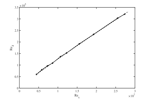
Figure 2: Non-dimensional boundary layer thickness $U_{e}\delta/\nu$ as a function of the non-dimensional downstream distance $Re_{x}=U_{e}x/\nu$. Circles: experimental data from Marusic (2015) (the SP40 configuration); Dashed line: Theoretical prediction of equation 79.

Figures 1 and 2 show that with these numerical values of the coefficients, the theoretical prediction has an excellent agreement with the experimental results. It is interesting to note that the values of the von Kármán constant obtained is different from the value of $0.384$ obtained in the same experiment and by Nagib et al. (2007), but much closer to that of Vallikivi et al. (2015) (0.40) and the typical value of 0.421 in pipe flows (McKeon et al. 2004; McKeon & Morrison 2007). We emphasize that these are preliminary comparisons with a single set of experimental data. Nevertheless, they might still shed some light on the way in which the von Kármán constant is determined from the velocity profile and needs further attention.

Here we also provide a list of predictions to be evaluated using experimental data in future works.

1. Comprehensive assessment of the downstream evolution of the friction velcity and the boundary layer thickness. In particular, the virtual origion, the von Kármán constant and the non-dimensional coefficients in 78 and 79 should be evaluated.

2. The logarithmic friction law 75. Note that there are no higher-order corrections to this law. Therefore, when plotting $U_{e}/u_{*}$ vs $\ln(u_{*}^{2}x/U_{e}\nu)$, a straightlie should extend down to relatively modest Reynolds numbers. Such comparisons will also provide another evaluation of the von Kármán constant

3. Comprehensive evaluation of the expansion coefficients in the asymptotic expansions 73 or 74 of velocity profile in the overlapping region. The extent of the log region can be evaluated and comparisons with channel flows can be made.

4. A new evaluation of the von Kármán constant using the measured mean velocity profile and the predicted higher-order prediction in the overlapping region (log law plus the higher-order corrections), rather than the log law alone, as done previously. This allows determination of the constant using data obtained at moderate Reynolds numbers, rather than chasing the seemingly ellusive high Reynolds numbers.

5. Comprehensive evaluation of the expansion coefficients in the asymptotic expansions 76 or 77 of Reynolds shear-stress profile in the overlapping region.

4 Discussions

The asymptotic expansions are an approximate solution of the boundary layer equations in the matching layer. They allow us to compare and contrast ZPGTBL with channel flows. In channel flows (and pipe flows), the leading-order mean momentum equation in the outer layer is a balance between the shear stress derivative and the mean pressure gradient (Afzal 1976), with the latter imposing the linear variation of the leading-order (linear) variation of the Reynolds shear stress. The Reynolds shear-stress budget is a balance between shear production and velocity-gradient–pressure interaction. While the mean velocity itself does not appear in the mean momentum equation, the mean velocity gradient is “adjusted” to balance the Reynolds stress budget. This is where the constant stress condition is needed for the log law (through the pressure-strain-rate correlation).

In ZPGTBL the leading-order mean momentum balance is between the mean advection due to the free-stream velocity $U_{e}$ and the shear stress derivative. The leading-order (linear) variation of the Reynolds shear stress results from the log law. It is interesting to observe that while the non-dimensional leading-order Reynolds shear stress derivative equals $1/\kappa$, the leading-order shear stress in the boundary layer can be written as

$$\overline{uv}=u_{*}^{2}\Big{\{}-1+\frac{1}{\kappa}y_{o}\Big{\}}=u_{*}^{2}\Big{\{}-1+\frac{0.3659}{\kappa}\frac{y}{\delta_{99}}\Big{\}}.$$ (81)

The coefficient for the second term on the r.h.s. is not very different from the value of one in channel flows. The mean advection depends on the growth of the boundary layer thickness and the variations of $u_{*}$; therefore the mean momentum balance is more delicate. The Reynolds shear stress balance is among the mean advection, production and velocity gradient-pressure interaction respectively. Again, due to the mean advection, the balance is also more delicate. However, in the near-wall region ($y_{o}\ll 1$), the advection term is of higher-order. Therefore the Reynolds shear stress balance is similar to that in channel flows.

The functional forms of the leading-order terms for both the outer ($U_{o}=(1/\kappa)\ln y_{o}+C+A_{u}y_{o}$) and inner expansions ($U_{i}=(1/\kappa)\ln y^{+}+B+C_{u}(y^{+})^{-1}$) are identical for channel flows and ZPGTBL. Therefore the von Kármán constant and the extent of the log layer at the leading order should be asymptotically identical for both flows. Physically this is because the leading-order scaling of the turbulence fluctuations (e.g., the velocity variances and the pressure-strain-rate correlation) are the essentially same for both channel flows and the boundary layer. Therefore, there is no reason to believe that the log law would not be universal. However the values of $A_{u}$ and $C_{u}$ determine the onset of the log layer, i.e., the lowest $y^{+}$ and the highest $y/\delta$ values for the log layer. Given that the leading-order Reynolds shear-stress budget contains an advection term, we might expect $A_{u}$ to be different from its counterpart in channel flows.

In channel flows, the lowest (second-order) order correction terms to (or deviations from) the leading-order terms are of order $Re_{*}^{-1}$ in both the outer and inner layers, whereas in ZPGTBL they are of order $u_{*}/U_{e}\sim\ln^{-1}Re_{*}$ in the outer layer, larger than in channel flows, and are of order $Re_{\delta}^{-1}$ in the inner layer, smaller than in channel flows. This suggests that the deviations from the leading order are larger toward the outer layer and smaller toward the inner layer in ZPGTBL than in channel flows.

In channel flows there is a second-order (and more at the higher orders) logarithmic term in the mean velocity (Afzal 1976), indicating that the observed coefficient for the logarithmic part of the profile, which is usually taken as the (apparent) von Kármán constant, is Reynolds-number dependent. Note that the von Kármán constant is defined as the coefficient for the leading-order logarithmic profile. Such a term is absent in ZPGTBL. As a result, at finite Reynolds numbers we will observe departures from the log law in ZPGTBL, rather than a Reynolds-number-dependent (apparent) von Kármán constant.

The physics related to the corrections are also different in the two flows. In channel flows it is due to (higher-order) viscous effects in the outer layer and (higher-order) variations of the shear stress in the inner layer respectively. The former depends explicitly on the Reynolds number whereas the latter has an implicit dependence through other variables (variations of the shear stress). In ZPGTBL, the leading-order the corrections in the outer layer are caused by the advection due to the velocity defect, advection due to the wall-normal mean velocity, and the streamwise derivative of the velocity variance differences. The dependence of the Reynolds number is implicit, through the effects of the Reynolds number on the growth of the boundary layer thickness and the variations of $u_{*}$, as none of the variables are directly dependent on the viscosity. In the inner layer, the corrections are caused by advection due to the vertical velocity.

The leading-order logarithmic friction law for channel flows is accurate to $O(Re_{*}^{-1})$. For ZPGTBL, equation 75 indicates that it is accurate, without any higher-order corrections. Therefore, the logarithmic friction law is more accurate in ZPGTBL than in channel flows.

5 Conclusions

We performed a symmetry analysis of the equations for ZPGTBL using Lie dilation groups, and obtained local, leading-order symmetries of the equations. The full set of similarity variables was obtained from the characteristic equations of the group. The dependent similarity variables, which are generally functions of the independent similarity variable (the local non-dimensional normal coordinate) and Reynolds numbers, were written as asymptotic expansions, with the gauge functions depending on the Reynolds numbers. Using the asymptotic expansions the perturbation equations for the outer and inner layers were obtained and the gauge functions were determined. Matching the expansions resulted in an approximate similarity solution of ZPGTBL in the overlapping layer. Expansion terms up to the third order were obtained. To our best knowledge, these results have not been obtained previously. Furthermore, they were obtained from first principles without any major assumptions. The main results are as follows.

1. We showed that similar to the Navier-Stokes equations at high Reynolds numbers (turbulent flows), the Reynolds-averaged boundary layer equations for ZPGTBL do not have global symmetries, only have local, approximate symmetries. We obtained the leading-order Lie dilation symmetries, i.e., invariance under Lie dilation groups, in both the outer and inner layers.

2. We showed that the friction $u_{*}$ is the scale for the velocity defect. Using the free-stream $U_{e}$ as the scale, as suggested by some previous studies, would lead to an inconsistency with the scaling of the TKE dissipation rate.

3. We derived analytically from the boundary layer equations the non-dimensional friction velocity $u_{*}/U_{e}$ and the non-dimensional boundary layer thickness $U_{e}\delta/\nu$ as functions of the non-dimensional downstream distance $U_{e}x/\nu$ using the characteristic equations of the group. When using the von Kármán constant, the virtual origin of the boundary layer, and two non-dimensional coefficients determined from the experimental data of Marusic et al. (2015), the theoretical prediction shows excellent agreement with the data.

4. From the symmetry analysis, the independent similarity variable for the outer layer wall-normal coordinate was obtained using the boundary layer parameters as $y_{o}=yU_{e}/(xu_{*})$, analogous to that in the Blasius boundary layer. Previously the non-dimensionalising variable was not fully defined, i.e., not using the boundary layer parameters.

5. The leading-order similarity equations, which are ordinary differential equations, were obtained. The dependent similarity variables, written as asymptotic expansions, were used to derive the perturbation equations, which also contain the higher-order similarity equations and have not been obtained previously. The gauge functions for the outer layer are determined as $u_{*}/U_{e}$, $Re_{*}^{-1}$, $u_{*}^{2}/U_{e}^{2}$, … Those for the inner layer are $Re_{\delta}^{-1}$, $Re_{\delta}^{-1}u_{*}/U_{e}$, … These gauge functions are in contrast to those for channel flows, which are $Re_{*}^{-1}$, $Re_{*}^{-2}$, …, for both the outer and inner layers. The approximate solution in the overlapping layer as asymptotic expansions were obtained. Using the method of matched asymptotic expansions to obtain an approximate solution avoided a turbulence model.

6. While the leading-order outer equations for ZPGTBL are different from those for channel flows, the leading-order expansion terms in the overlapping layer are formally identical. This result provides analytic support to the notion that the log law and the broader leading-order mean flow are asymptotically universal in this layer.

7. The higher-order expansions for the ZPGTBL and channel flows are different. With the log law at the leading order in ZPGTBL without any other logarithmic terms, the logarithmic friction law is accurate. By contrast, in channel flows it has a logarithmic term at the second order. Therefore the friction law is only accurate at the leading order.

8. The second-order corrections to the leading-order outer-layer expansions are asymptotically larger in ZPGTBL than in channel flows, whereas those to the leading-order inner-layer expansions are smaller in ZPGTBL than in channel flows. Due to these differences, we might expect the onset and possibly the extent of the logarithmic profile in measurements and simulations to be different. This issue will be investigated in a future work.

The asymptotic expansions obtained in the present work will also provide a more systematic approach to assess the asymptotic behaviours of ZPGTBL using experimental data. For example, the log law is often investigated using the measured mean velocity profile. While the mean profile exhibits an approximate logarithmic dependence only at sufficiently high Reynolds numbers, the log law is a leading-order term in the profile, a result of matching the leading-order outer and inner profiles with the same velocity scale (Tong & Ding 2020). It is present even at moderate Reynolds numbers. At such Reynolds numbers it may be obscured by the other leading-order and higher-order terms in the mean velocity profile. However, in principle it can be obtained experimentally by determining the coefficients of the other terms in 73, e.g., using measurements at several Reynolds numbers and then subtracting these terms from the mean profile. The issue of the asymptotic scaling of ZPGTBL perhaps could be better addressed through collaboration among the theoretical and experimental groups.

Declaration of Interests. The authors report no conflict of interest.

Acknowledgments

The author thanks Professors Zellman Warhaft and Katepalli Sreenivasan for reading the manuscript and for providing valuable comments. He is also thankful to Professor Sreenivasan for encouraging him to look into issues in classical engineering turbulent boundary layers. This work was supported by the National Science Foundation under grant AGS-2054983.

Appendix A Derivation of the outer and inner layer perturbation equations

Equation 17 suggests that $\Delta_{1}=u_{*}/U_{e}\approx\ln^{-1}Re_{*}$, which is confirmed by 89. It also shows that $\Delta_{2}=Re_{*}^{-1}$. With these gauge functions the perturbation and similarity equations for the mean momentum equation in the outer layer are derived as follows.

$$\frac{\partial U}{\partial x}=\frac{du_{*}}{dx}U_{o}+u_{*}\frac{d}{dx}\Big{\{}U_{o_{1}}+\Delta_{1}U_{o_{2}}+Re_{*}^{-1}U_{o_{3}}+\Delta_{3}(Re_{*})U_{o_{2}}(y_{o})\Big{\}},$$ (82)

where

$$\begin{split}\frac{d}{dx}\Big{\{}U_{o_{1}}+\Delta_{1}U_{o_{2}}\Big{\}}=\frac{dU_{o_{1}}}{dy_{o}}yU_{e}(\frac{-1}{x^{2}u_{*}}+\frac{-1}{xu_{*}}\frac{du_{*}}{dx})+\frac{d\Delta_{1}}{dx}U_{o_{2}}+\Delta_{1}\frac{dU_{o_{2}}}{dy_{o}}yu_{e}\\ =\frac{dU_{o1}}{dy_{o}}(\frac{-y_{o}}{x}+\frac{-y_{o}}{u_{*}}\frac{du_{*}}{dx})+\frac{1}{U_{e}}\frac{du_{*}}{dx}U_{o2}+\Delta_{1}\frac{dU_{o2}}{dy_{o}}(\frac{-y_{o}}{x}+\frac{-y_{o}}{u_{*}}\frac{du_{*}}{d_{x}}).\end{split}$$ (83)

The non-dimensional form of its contribution to the advection is

$$\begin{split}\frac{x}{U_{e}u_{*}}U_{e}u_{*}\frac{d}{dx}\Big{\{}U_{o_{1}}+\Delta_{1}U_{o_{2}}\Big{\}}=\frac{dU_{o_{1}}}{dy_{o}}(-y_{o}-\frac{x}{u_{*}}y_{o}\frac{du_{*}}{dx})+\frac{x}{U_{e}}\frac{du_{*}}{dx}U_{o2}+\Delta_{1}\frac{dU_{o2}}{dy_{o}}(y_{o}+\frac{x}{u_{*}}y_{o}\frac{du_{*}}{dx})\end{split}$$

$$\begin{split}=\frac{dU_{o1}}{dy_{o}}(-y_{o}+\frac{y_{o}}{\kappa\frac{U_{e}}{u_{*}}+2})-\frac{u_{*}}{U_{e}}\frac{U_{o2}}{\kappa\frac{U_{e}}{u_{*}}+2}+\Delta_{1}\frac{dU_{o2}}{dy_{o}}(-y_{o}+\frac{y_{o}}{\kappa\frac{U_{e}}{u_{*}}+2}).\end{split}$$ (84)

The term

$$\frac{1}{\kappa\frac{U_{e}}{u_{*}}+2}=\frac{u_{*}}{\kappa U_{e}}-2\Big{(}\frac{u_{*}}{\kappa U_{e}}\Big{)}^{2}+...,$$ (85)

and therefore contains both $\Delta_{1}$ and $\Delta_{3}$. The $U_{o3}$ term is

$$\begin{split}\frac{d}{dx}(Re_{*}^{-1}U_{o3})=\frac{dRe_{*}^{-1}}{dx}U_{o3}+Re_{*}^{-1}\frac{dU_{o3}}{dx}\\ =-Re_{*}^{-2}\frac{dRe_{*}}{dx}+Re_{*}^{-1}\frac{dU_{o3}}{dy_{o}}yU_{e}(\frac{-1}{x^{2}u_{*}}+\frac{-1}{xu_{*}^{2}}\frac{du_{*}}{dx})\\ =-Re_{*}^{-2}\frac{U_{o_{3}}}{\nu}\frac{1}{U_{e}}(u^{2}_{*}+2xu_{*}\frac{du_{*}}{dx})+Re_{*}^{-1}\frac{dU_{o3}}{dy_{o}}yU_{e}(\frac{-1}{x^{2}u_{*}}+\frac{-1}{xu_{*}^{2}}\frac{du_{*}}{dx}).\end{split}$$ (86)

Its non-dimensional form is

$$\begin{split}\frac{x}{U_{o}u_{*}}U_{e}u_{*}\frac{dRe_{x}^{-1}U_{o3}}{dx}=-\frac{u_{*}xRe_{*}^{-2}}{u_{*}}\frac{U_{o3}}{\nu}(u_{*}^{2}+2xu_{*}\frac{du_{*}}{dx})+\\ \frac{U_{e}xu_{*}}{U_{e}u_{*}}Re_{*}^{-1}\frac{dU_{o3}}{dy_{o}}yU_{e}(\frac{-1}{x^{2}u_{*}}+\frac{-1}{xu_{*}^{2}}\frac{du_{*}}{dx})-\\ =-Re_{*}^{-2}U_{o3}\big{(}\frac{u_{*}^{2}}{U_{e}}\frac{x}{\nu}+\frac{2x^{2}u_{*}}{U_{e}\nu}\frac{(-u_{*})}{x(\frac{\kappa kU_{e}}{u_{*}}+2)}\big{)}+\\ =-Re_{*}^{-2}U_{o3}\big{(}Re_{*}+Re_{*}\frac{-2}{\frac{\kappa U_{e}}{u_{*}}+2}\big{)}+Re_{*}^{-1}\frac{dU_{o_{3}}}{dy_{o}}\big{(}-y_{o}+\frac{y_{o}}{\frac{kU_{e}}{u_{*}}+2}\big{)}.\end{split}$$

The $U_{o4}$ term is

$$\frac{d\Delta_{3}U_{o_{4}}}{dx}=\frac{d\Delta_{3}}{dx}U_{o4}+\Delta_{3}\frac{dU_{o_{4}}}{dx}=\Delta^{{}^{\prime}}_{3}\frac{Re_{x}}{dx}U_{o4}+\Delta_{3}\frac{dU_{o_{4}}}{dx},$$ (87)

with the non-dimensional form

$$\begin{split}\frac{xU_{e}}{U_{e}u_{*}}U_{e}u_{*}\frac{d\Delta_{3}U_{o4}}{dx}=x\Delta^{{}^{\prime}}_{3}\frac{dRe_{x}}{dx}U_{o_{4}}+x\Delta_{3}\frac{dU_{o_{4}}}{dx}\\ =x\Delta^{{}^{\prime}}_{3}\frac{U_{o_{4}}}{U_{e}\nu}\big{(}u_{x}^{2}+2xu_{x}\frac{-u_{x}}{x(\frac{kU_{e}}{u_{x}}+2)}\big{)}+\Delta_{3}\frac{dU_{o_{4}}}{dy_{o}}\big{(}-y_{o}+\frac{y_{o}}{\frac{kU_{e}}{u_{x}}+2}\big{)}\\ =\Delta^{{}^{\prime}}_{3}Re_{x}U_{o_{4}}\big{(}1+\frac{-2}{\frac{kU_{e}}{u_{x}}+2}\big{)}+\Delta_{3}\frac{dU_{o_{4}}}{dy_{o}}\big{(}-y_{o}+\frac{y_{o}}{\frac{kU_{e}}{u_{x}}+2}\big{)}.\\ \end{split}$$ (88)

The non-dimensional advection term due to the velocity defect is

$$\frac{x}{U_{e}u_{x}}(U-U_{e})\frac{\partial U}{\partial x}=\frac{x}{U_{e}u_{*}}u_{*}U_{o}\frac{\partial U}{\partial x}=\frac{x}{U_{e}}U_{o}\frac{\partial U}{\partial x}$$

$$\begin{split}=\frac{x}{U_{e}}U_{o}\Big{\{}(U_{o_{1}}+\Delta_{1}U_{o_{2}})\frac{du_{x}}{dx}+u_{*}\frac{dU_{o_{1}}+\Delta_{1}U_{o_{2}}}{dx}\\ +(Re^{-1}_{*}U_{o_{3}}+\Delta_{2}U_{o_{4}})\frac{du_{*}}{dx}+u_{*}\frac{d}{dx}(Re^{-1}_{*}U_{o_{3}}+\Delta_{3}U_{o_{4}})\Big{\}}\\ =\frac{u_{*}}{U_{e}}\big{(}U_{o_{1}}+\Delta_{1}U_{o_{2}}+Re^{-1}_{*}U_{o_{3}}+\Delta_{3}U_{o_{4}}\big{)}^{2}\frac{-1}{k\frac{U_{e}}{u_{x}}+2}\\ +\frac{u_{*}}{U_{e}}\Big{\{}\frac{dU_{o1}}{dy_{o}}(-y_{o}+\frac{y_{o}}{\kappa\frac{U_{e}}{u_{*}}+2})-\frac{u_{*}}{U_{e}}\frac{U_{o2}}{\kappa\frac{U_{e}}{u_{*}}+2}+\Delta_{1}\frac{dU_{o2}}{dy_{o}}(-y_{o}+\frac{y_{o}}{\kappa\frac{U_{e}}{u_{*}}+2})\Big{\}}\end{split}$$

$$\begin{split}-\frac{u_{*}}{U_{e}}U_{o}Re^{-1}_{*}U_{o_{3}}\big{(}1+\frac{2}{k\frac{U_{e}}{u_{*}}+2}\big{)}+\frac{u_{*}}{U_{e}}U_{o}Re^{-1}_{*}U_{o_{3}}\frac{dU_{o_{3}}}{dy_{o}}\big{(}-y_{o}+\frac{y_{o}}{k\frac{U_{e}}{u_{x}}+2}\big{)}.\\ \end{split}$$ (89)

Equation 89 shows that

$$\Delta_{3}=\big{(}\frac{u_{*}}{U_{e}}\big{)}^{2}=\frac{1}{\ln^{2}Re_{*}}.\$$ (90)

Thus

$$\Delta_{3}^{{}^{\prime}}=\frac{-2}{\ln^{3}Re_{*}}\frac{d\ln Re_{*}}{dRe_{*}}.\ =\frac{-2}{\ln^{3}Re_{*}}\frac{1}{Re_{*}}.$$ (91)

The advection due to the normal velocity is obtained as

$$\frac{dU}{dy}=u_{*}\frac{dU_{o}}{dy}\frac{dy_{o}}{dy}=u_{*}\frac{dU_{o}}{dy_{o}}\frac{U_{e}}{u_{*}x},$$ (92)

$$V\frac{\partial U}{\partial y}=\frac{u_{*}^{2}}{U_{e}}V_{o}\frac{dU_{o}}{dy_{o}}\frac{U_{e}}{x}=\frac{u_{*}^{2}}{x}V_{o}\frac{dU_{o}}{dy_{o}},$$ (93)

and

$$\frac{x}{U_{e}u_{*}}\frac{u_{*}^{2}}{x}V_{o}\frac{dU_{e}}{dy_{o}}=\frac{u_{*}}{U_{e}}V_{o}\frac{dU_{o}}{dy_{o}}.$$ (94)

The shear-stress derivative is

$$\begin{split}\frac{d\overline{uv}}{dy}=u_{*}^{2}\frac{d\overline{uv}_{o}}{dy_{o}}\frac{dy_{o}}{dy}=u_{*}^{2}\frac{d\overline{uv_{o}}}{dy_{o}}\frac{U_{e}}{xu_{*}},\\ \frac{x}{U_{e}u_{*}}\frac{d\overline{uv}}{dy}=\frac{x}{U_{e}u_{*}}u_{*}^{2}\frac{d\overline{uv_{o}}}{dy_{o}}\frac{v_{e}}{xu_{*}}=\frac{d\overline{uv_{o}}}{dy_{o}}.\end{split}$$ (95)

The viscous term is

$$\nu\frac{\partial^{2}U}{\partial y^{2}}=\nu\frac{U_{e}}{x}\frac{\partial^{2}U_{o}}{\partial y_{o}^{2}}\frac{U_{e}}{xu_{*}},$$ (96)

$${\frac{x}{U_{e}u_{*}}}\nu{\frac{U_{e}}{x}}\frac{\partial^{2}U_{o}}{\partial y_{o}^{2}}\frac{U_{e}}{xu_{*}}=\frac{\nu}{xu_{*}}\frac{U_{e}}{u_{*}}\frac{\partial^{2}U_{o}}{\partial y_{o}^{2}}=\frac{\nu}{\partial u_{*}}\frac{\partial^{2}U_{o}}{\partial y_{o}^{2}}=Re_{*}^{-1}\frac{\partial^{2}U_{o}}{\partial y_{o}^{2}}.$$ (97)

The derivative of the normal stress difference is

$$\begin{split}\frac{\partial u_{*}^{2}(\overline{u_{o}^{2}}-\overline{v_{o}^{2}})}{\partial x}=2u_{*}\frac{\partial u_{*}}{dx}(\overline{u_{o}^{2}}-\overline{v_{o}^{2})}+u_{*}^{2}\frac{\partial}{\partial x}\big{(}\overline{u_{o1}^{2}}-\overline{v_{o1}^{2}}+\Delta_{1}(\overline{u_{o2}^{2}}-\overline{v_{o2}^{2}})+...\big{)}\\ =2u_{*}\frac{\partial u_{*}}{dx}(\overline{u_{o}^{2}}-\overline{v_{o}^{2})}+u_{*}^{2}\frac{d(\overline{u_{o1}^{2}}-\overline{v_{o1}^{2}})}{dy_{o}}yU_{e}\big{(}\frac{-1}{x^{2}u_{*}}-{\frac{1}{xu_{*}^{2}}\frac{\partial u_{*}}{\partial x}}\big{)}\\ +u_{*}^{2}\frac{d\Delta_{1}}{dx}(\overline{u_{o2}^{2}}-\overline{v_{o2}^{2}})+u_{*}^{2}\frac{d(\overline{u_{o2}^{2}}-\overline{v_{o2}^{2}})}{dy_{o}}yU_{e}\big{(}\frac{-1}{x^{2}u_{*}}-{\frac{1}{xu_{*}^{2}}\frac{\partial u_{*}}{\partial x}}\big{)}.\end{split}$$ (98)

Its non-dimensional form is

$$\begin{split}\frac{x}{U_{e}u_{*}}\frac{\partial(\overline{u^{2}}-\overline{v^{2}})}{\partial x}=2\frac{x}{U_{e}}\frac{du_{*}}{dx}(\overline{u_{o}^{2}}-\overline{v_{o}^{2}})+\frac{{x}}{U_{e}{u_{*}}}u_{*}^{2}yU_{e}\big{(}\frac{-1}{x^{2}u_{*}}-{\frac{1}{xu_{*}^{2}}\frac{du_{*}}{dx}}\big{)}\frac{d(\overline{u_{o1}^{2}}-\overline{v_{o1}^{2}})}{dy_{o}}\\ +\frac{x}{U_{e}u_{*}}u_{*}^{2}\frac{-u_{*}}{U_{e}x}\frac{\overline{u_{o2}^{2}}-\overline{v_{o2}^{2}}}{\kappa\frac{U_{e}}{u_{*}}+2}++\frac{u_{*}}{U_{e}}\big{(}\frac{u_{*}}{U_{e}}y_{o}+\frac{u_{*}}{U_{e}}y_{o}\frac{1}{\kappa\frac{U_{e}}{u_{*}}+2}\big{)}\frac{d(\overline{u_{o2}^{2}}-\overline{v_{o2}^{2}})}{dy_{o}}\\ =-2\frac{u_{*}}{U_{e}}\frac{(\overline{u_{o}^{2}}-\overline{v_{o}^{2}})}{k\frac{U_{e}}{u_{*}}+2}+\frac{u_{*}}{U_{e}}\big{(}-y_{o}+\frac{1}{k\frac{U_{e}}{u_{*}}+2}\big{)}\frac{d(\overline{u_{o1}^{2}}-\overline{v_{o1}^{2}})}{dy_{o}}+\frac{U_{e}^{2}}{u_{*}^{2}}\frac{(\overline{u_{o2}^{2}}-\overline{v_{o2}^{2}})}{k\frac{U_{e}}{u_{*}}+2}\\ +\frac{u_{*}^{2}}{U_{e}^{2}}\big{(}-y_{o}+\frac{1}{k\frac{U_{e}}{u_{*}}+2}\big{)}\frac{d(\overline{u_{o2}^{2}}-\overline{v_{o2}^{2}})}{dy_{o}}.\end{split}$$ (99)

Using 84, 86, 88, 89, 94, 95, 97, 99, and 1, we obtain the non-dimensional outer momentum equation 58.

The outer shear-stress budget are obtained as follows.

$$\begin{split}\frac{\partial\overline{uv}}{\partial x}=\overline{uv_{o}}\frac{\partial u_{*}^{2}}{\partial x}+u_{*}^{2}\frac{\partial\overline{uv_{o}}}{\partial x}=2\overline{uv}_{o}u_{*}\frac{-u_{*}}{x({k\frac{U_{e}}{u_{*}}+2})}\\ +u_{*}^{2}\Big{\{}\frac{d\overline{uv}_{o}}{dy_{o}}yU_{e}(\frac{-1}{x^{2}u_{*}}+\frac{-1}{xu_{*}^{2}}\frac{du_{*}}{dx})+\frac{d\Delta_{1}}{dx}\overline{uv_{o_{2}}}+\Delta_{1}{\frac{d\overline{uv_{o_{2}}}}{dy_{o}}yU_{e}(\frac{-1}{x^{2}u_{*}}+\frac{-1}{xu_{*}^{2}}\frac{du_{*}}{dx})}\\ +\frac{d}{dx}(Re_{*}^{-1}\overline{uv}_{o2})+\frac{d\Delta_{3}\overline{uv}_{o4}}{dx}\Big{\}}.\\ \end{split}$$ (100)

Its non-dimensional form up to the order of $\Delta_{1}$ is

$$\frac{x}{U_{e}u_{*}^{2}}U_{e}\frac{\partial\overline{uv}}{\partial x}=-\frac{2\overline{uv}_{o}}{k\frac{U_{e}}{u_{*}}+2}+\frac{d\overline{uv}_{o1}}{dy_{o}}y_{o}(-1+\frac{1}{{k\frac{U_{e}}{u_{*}}+2}})-\frac{u_{*}}{U_{e}}\frac{\overline{uv}_{o2}}{k\frac{U_{e}}{u_{*}}+1}+\frac{u_{*}}{U_{e}}\frac{d\overline{uv}_{02}}{dy_{o}}(y_{o}+\frac{y_{o}}{k\frac{U_{e}}{u_{*}}+2}).$$ (101)

The order $Re_{*}$ term is

$$\begin{split}\frac{d}{dx}(Re_{*}^{-1}\overline{uv}_{o2})=\frac{dRe_{*}^{-1}}{dx}\overline{uv}_{o3}+Re_{*}^{-1}\frac{\overline{uv}_{o2}}{dx}\\ =-Re_{*}^{-2}\frac{dRe_{*}}{dx}\overline{uv}_{o3}+Re_{*}^{-1}\frac{d\overline{uv}_{o3}}{dy_{o}}yU_{e}(\frac{-1}{x^{2}u_{*}}+\frac{-1}{xu_{*}^{2}}\frac{du_{*}}{dx})\\ =-Re_{*}^{-2}\frac{\overline{uv}_{o3}}{\nu}\frac{1}{U_{e}}(u^{2}_{*}+2xu_{*}\frac{du_{*}}{dx})+Re_{*}^{-1}\frac{d\overline{uv}_{o3}}{dy_{o}}yU_{e}(\frac{-1}{x^{2}u_{*}}+\frac{-1}{xu_{*}^{2}}\frac{du_{*}}{dx}).\end{split}$$ (102)

The non-dimensional form is

$$\begin{split}\frac{x}{U_{o}u_{*}}U_{e}u_{*}\frac{dRe_{x}^{-1}\overline{uv}_{o3}}{dx}=-\frac{u_{*}xRe_{*}^{-2}}{u_{*}}\frac{\overline{uv}_{o3}}{\nu}(u_{*}^{2}+2xu_{*}\frac{du_{*}}{dx})+\\ \frac{U_{e}xu_{*}}{U_{e}u_{*}}Re_{x}^{-1}\frac{d\overline{uv}_{o3}}{dy_{o}}yU_{e}(\frac{-1}{x^{2}u_{*}}+\frac{-1}{xu_{*}^{2}}\frac{du_{*}}{dx})\\ =-Re_{x}^{-1}\overline{uv}_{o3}\big{(}1+\frac{-2}{\frac{\kappa U_{e}}{u_{*}}+2}\big{)}+Re_{*}^{-1}\frac{d\overline{uv}_{o3}}{dy_{o}}\big{(}-y_{o}+\frac{y_{o}}{\frac{kU_{e}}{u_{*}}+2}\big{)}.\end{split}$$ (103)

The order $\Delta_{3}$ term is

$$\frac{d\Delta_{3}\overline{uv}_{o4}}{dx}=\frac{d\Delta_{3}}{dx}\overline{uv}_{o4}+\Delta_{3}\frac{d\overline{uv}_{o4}}{dx}=\Delta^{{}^{\prime}}_{3}\frac{dRe_{x}}{dx}\overline{uv}_{o4}+\Delta_{3}\frac{d\overline{uv}_{o4}}{dx},$$ (104)

with the non-dimensional form

$$\begin{split}\frac{xU_{e}}{U_{e}u_{*}}U_{e}u_{*}\frac{d\Delta_{3}\overline{uv}_{o4}}{dx}=x\Delta^{{}^{\prime}}_{3}\frac{dRe_{x}}{dx}\overline{uv}_{o4}+x\Delta_{3}\frac{d\overline{uv}_{o4}}{dx}\\ =x\Delta^{{}^{\prime}}_{3}\frac{\overline{uv}_{o4}}{U_{e}\nu}\big{(}u_{x}^{2}+2xu_{x}\frac{-u_{x}}{x(\frac{kU_{e}}{u_{x}}+2)}\big{)}+\Delta_{3}\frac{d\overline{uv}_{o4}}{dy_{o}}\big{(}-y_{o}+\frac{y_{o}}{\frac{kU_{e}}{u_{x}}+2}\big{)}\\ =-2\frac{u_{*}^{3}}{U_{e}^{3}}\overline{uv}_{o4}\big{(}1+\frac{-2}{\frac{kU_{e}}{u_{x}}+2}\big{)}+\frac{u_{*}^{2}}{U_{e}^{2}}\frac{d\overline{uv}_{o4}}{dy_{o}}\big{(}-y_{o}+\frac{y_{o}}{\frac{kU_{e}}{u_{x}}+2}\big{)}.\\ \end{split}$$ (105)

The advection due to the velocity defect is

$$\begin{split}\frac{x}{U_{e}u_{*}^{2}}(U-U_{e})\frac{\partial\overline{uv}}{\partial x}=-\frac{u_{*}}{U_{e}}\frac{2U_{o}\overline{uv_{o}}}{k\frac{U_{o}}{u_{*}}+2}+\frac{u_{*}}{U_{e}}U_{o}\frac{d\overline{uv}_{o2}}{dy_{o}}y_{o}(-1+\frac{1}{\frac{kU_{e}}{u_{x}}+2})+(\frac{u_{*}}{u_{e}})^{2}U_{o_{1}}\frac{-2\overline{uv}_{o2}}{\frac{kU_{e}}{u_{x}}+2}\\ -\frac{u_{*}^{2}}{U_{e}^{2}}U_{o1}\frac{d\overline{uv}_{o2}}{dy_{o}}(-1+\frac{-1}{\frac{kU_{e}}{u_{x}}+2}).\\ \end{split}$$ (106)

The advection due to the normal velocity is

$$\begin{split}\frac{\partial\overline{uv}}{\partial y}=u_{*}^{2}\frac{\partial\overline{uv_{o}}}{\partial y_{o}}\frac{U_{e}}{xu_{*}},\ \ V\frac{\partial\overline{uv}}{\partial y}=\frac{u_{*}^{2}}{U_{e}}V_{o}u_{*}^{2}\frac{\partial\overline{uv_{o}}}{\partial y_{o}}\frac{U_{e}}{xu_{*}}\\ \frac{x}{U_{e}u_{*}^{2}}V\frac{\partial\overline{uv}}{\partial y}=\frac{u_{*}}{U_{e}}V_{o}\frac{\partial\overline{uv_{o}}}{\partial y_{o}}.\\ \end{split}$$ (107)

The shear-stress production is

$$\begin{split}\overline{v_{o}^{2}}\frac{\partial U}{\partial y}=u_{*}^{2}v_{o}^{2}u_{*}\frac{\partial U_{o}}{\partial y_{o}}\frac{U_{e}}{xu_{*}},\\ \frac{x}{U_{e}u_{*}^{2}}\overline{v^{2}}\frac{\partial U}{\partial y}=\overline{v_{o}^{2}}\frac{\partial U_{o}}{\partial y_{o}}.\end{split}$$ (108)

The viscous diffusion is

$$\begin{split}\frac{\partial^{2}\overline{uv}}{\partial y^{2}}=u_{*}^{2}\frac{\partial^{2}\overline{uv_{o}}}{dy_{o}^{2}}(\frac{U_{e}}{xu_{*}^{2}}),\\ \frac{x}{U_{e}u_{*}^{2}}\nu\frac{\partial^{2}\overline{uv}}{\partial y^{2}}=\frac{x\nu}{U_{e}u_{*}^{2}}\frac{U_{e}^{2}}{x^{2}}\frac{d^{2}\overline{uv}_{o}}{dy_{o}^{2}}=\frac{\nu}{u_{*}x}\frac{U_{e}}{u_{*}}\frac{\partial^{2}\overline{uv}_{o}}{dy_{o}^{2}}=\frac{\nu}{U_{e}\delta}\frac{U_{e}}{u_{*}}\frac{\partial^{2}\overline{uv_{o}}}{dy_{o}^{2}}=\frac{\nu}{u_{*}\delta}\frac{\partial^{2}\overline{uv}_{o}}{dy_{o}^{2}}.\end{split}$$ (109)

Combining the above terms we obtain the outer shear-stress budget 60.

The perturbation momentum equation for the inner is derived as follows.

$$\begin{split}\frac{\partial U}{\partial x}=\frac{\partial u_{*}U_{i}}{\partial x}=\frac{du_{*}}{dx}U_{i}+u_{*}\frac{\partial(U_{i1}+{\delta_{1}}U_{i2}+....)}{\partial x}\\ =\frac{du_{*}}{dx}U_{i}+u_{*}\Big{\{}\frac{dU_{i1}}{dy^{+}}\frac{dy^{+}}{dx}+\frac{d\delta_{1}}{dx}U_{i2}+\delta_{1}\frac{dU_{i2}}{dy^{+}}\frac{dy^{+}}{dx}+...\Big{\}}\\ =\frac{du_{*}}{dx}U_{i}+\frac{u_{*}y}{\nu}\big{(}\frac{du_{*}}{dx}\big{(}\frac{dU_{i1}}{dy^{+}}+\delta_{1}\frac{dU_{i2}}{dy^{+}}+...\big{)}+u_{*}\frac{d\delta_{1}}{dx}U_{i2},\\ \end{split}$$ (110)

where $dy^{+}/dx=(y/\nu)(du_{*}/dx)$. The non-dimensional advection due to $U$ is

$$\begin{split}\frac{\delta_{\nu}}{u_{*}^{2}}U\frac{\partial U}{\partial x}=\frac{\nu}{u_{*}^{3}}u_{*}U_{i}\Big{\{}\frac{du_{*}}{dx}U_{i}+\frac{u_{*}y}{\nu}\big{(}\frac{du_{*}}{dx}\big{(}\frac{dU_{i1}}{dy^{+}}+\delta_{1}\frac{dU_{i2}}{dy^{+}}+...\big{)}+u_{*}\frac{d\delta_{1}}{dx}U_{i2}\Big{\}}\\ =\frac{\nu}{u_{*}^{{2}}}U_{i}\Big{\{}\frac{-{u_{*}}U_{i}}{x(k\frac{U_{e}}{u_{*}}+2)}+y^{+}\frac{{-u_{*}}}{x(k\frac{U_{e}}{u_{*}}+2)}\big{(}\frac{dU_{i1}}{dy^{+}}+\delta_{1}\frac{dU_{i2}}{dy^{+}}+...\big{)}\Big{\}}\\ \sim\Big{\{}-\frac{\nu}{U_{e}\delta}U_{i}^{2}-\frac{\nu}{U_{e}\delta}y^{+}U_{i}\big{(}\frac{dU_{i1}}{dy+}+\delta_{1}\frac{dU_{i2}}{dy^{+}}+...\big{)}\Big{\}}\frac{1}{k\frac{U_{e}}{u_{*}}+2}\\ \sim Re_{\delta}^{-1}\frac{1}{k\frac{U_{e}}{u_{*}}+2}\Big{\{}-U_{i}^{2}-y^{+}U_{i}\big{(}\frac{dU_{i1}}{dy+}+\delta_{1}\frac{dU_{i2}}{dy^{+}}+...\big{)}\Big{\}},\end{split}$$ (111)

where $\nu/(u_{*}x)\approx\nu/(U_{e}\delta)$ has been used. The shear-stress derivative is

$$\frac{\partial\overline{uv}}{\partial y}=u_{*}^{2}\frac{\partial\overline{uv}_{i}}{\partial y^{+}}\frac{u_{*}}{\nu}.$$ (112)

The advection due to $V$ is

$$\frac{\partial U}{\partial y}=u_{*}\frac{\partial U_{i}}{\partial y^{+}}\frac{u_{*}}{\nu},\ \ \frac{\partial^{2}U}{\partial y^{2}}=u_{*}\frac{\partial^{2}U_{i}}{\partial y^{+2}}(\frac{u_{*}}{\nu})^{2},$$ (113)

$$V\frac{\partial U}{\partial y}=\frac{\nu}{\delta}\frac{u_{*}}{U_{e}}u_{*}V_{i}\frac{u_{*}^{2}}{\nu}\frac{\partial U_{i}}{\partial y^{+}},\ \ \frac{\delta_{\nu}}{u_{*}^{2}}V\frac{\partial U}{\partial y}=\frac{\nu}{\delta U_{e}}V_{i}\frac{\partial U_{i}}{\partial y^{+}}.$$ (114)

The normal-stress difference derivative is

$$\begin{split}\frac{\partial\overline{u^{2}}-\overline{v^{2}}}{\partial x}=\frac{\partial u_{*}U_{e}\overline{u_{i}^{2}}}{\partial x}-\frac{\partial u_{*}^{2}\overline{v_{i}^{2}}}{\partial x}=\frac{du_{*}}{dx}U_{e}\overline{u_{i}^{2}}+u_{*}U_{e}\frac{\partial\overline{u_{i}^{2}}}{\partial x}-\big{(}-2u_{*}\frac{du_{*}}{dx}\overline{v_{i}^{2}}+u_{*}^{2}\frac{\partial\overline{v_{i}^{2}}}{\partial x}\big{)}\\ =-\frac{u_{*}}{x}\frac{1}{k\frac{U_{e}}{u_{*}}+2}U_{e}\overline{u_{i}^{2}}+u_{*}U_{e}\frac{\partial\overline{u_{i}^{2}}}{\partial y^{+}}\frac{y}{\nu}\frac{du_{*}}{dx}-\big{(}2u_{*}\frac{u_{*}}{x}\frac{\overline{v_{i}^{2}}}{k\frac{U_{e}}{u_{*}}+2}+u_{*}^{2}\frac{d\overline{v_{i}^{2}}}{dy^{+}}\frac{y}{\nu}\frac{du_{*}}{dx}\big{)}\\ =-\frac{u_{*}}{x}\frac{1}{k\frac{U_{e}}{u_{*}}+2}U_{e}\overline{u_{i}^{2}}-u_{*}U_{e}\frac{y}{\nu}\frac{u_{*}}{x}\frac{1}{k\frac{U_{e}}{u_{*}}+2}\frac{\partial\overline{u_{i}^{2}}}{\partial y^{+}}-\big{(}-2u_{*}\frac{u_{*}}{x}\frac{\overline{v_{i}^{2}}}{k\frac{U_{e}}{u_{*}}+2}-u_{*}^{2}\frac{\partial\overline{u_{i}^{2}}}{\partial y^{+}}\frac{y}{\nu}\frac{u_{*}}{x}\frac{1}{k\frac{U_{e}}{u_{*}}+2}\big{)},\end{split}$$ (115)

where the scaling $\overline{u^{2}}\sim u_{*}^{2}\ln Re_{*}\sim u_{*}U_{e}$ (Townsend 1976) has been used. Its non-dimensional form is

$$\begin{split}\frac{\delta_{\nu}}{u_{*}^{2}}\frac{\partial\overline{u^{2}}-\overline{v^{2}}}{\partial x}=-\frac{\nu}{u_{*}^{2}}\frac{U_{e}}{x}\frac{\overline{u}_{i}^{2}}{k\frac{U_{e}}{u_{*}}+2}-\frac{\nu U_{e}}{u_{*}^{2}}\frac{y}{\nu}\frac{u_{*}}{x}\frac{1}{k\frac{U_{e}}{u_{*}}+2}\frac{\partial\overline{u_{i}^{2}}}{\partial y^{+}}-\Big{\{}-2\frac{\nu}{u_{*}}{x}\frac{v_{i}^{2}}{k\frac{U_{e}}{u_{*}}+2}-\frac{\nu}{u_{*}}\frac{y}{\nu}\frac{u_{*}}{x}\frac{1}{k\frac{U_{e}}{u_{*}}+2}\frac{\partial\overline{v_{i}^{2}}}{\partial y^{+}}\Big{\}}\\ =-\frac{\nu}{u_{*}\delta}\frac{\overline{u_{i}^{2}}}{k\frac{U_{e}}{u_{*}}+2}-\frac{\nu}{u_{*}\delta}\frac{1}{k\frac{U_{e}}{u_{*}}+2}y^{+}\frac{d\overline{u_{i}^{2}}}{dy^{+}}-\Big{\{}-2\frac{\nu}{U_{e}\delta}\frac{\overline{v_{i}^{2}}}{k\frac{U_{e}}{u_{*}}+2}-\frac{\nu}{U_{e}\delta}\frac{y^{+}}{k\frac{U_{e}}{u_{*}}+2}\frac{\partial\overline{v_{i}^{2}}}{\partial y^{+}}\Big{\}}\\ \approx-Re_{\delta}^{-1}\overline{u_{i}^{2}}-Re_{\delta}^{-1}y^{+}\frac{d\overline{u_{i}^{2}}}{dy^{+}}+2Re_{\delta}^{-1}\frac{u_{*}}{U_{e}}\overline{v_{i}^{2}}+Re_{\delta}^{-1}\frac{u_{*}}{U_{e}}y^{+}\frac{\partial\overline{v_{i}^{2}}}{\partial y^{+}}.\end{split}$$ (116)

The inner perturbation equation up to the order of $Re_{\delta}^{-1}u_{*}/U_{e}$ is

$$\begin{split}-Re_{\delta}^{-1}\frac{u_{*}}{U_{e}}\Big{\{}U_{i}^{2}+y^{+}\frac{dU_{i}}{dy^{+}}\Big{\}}+Re_{\delta}^{-1}V_{i}\frac{dU_{i}}{dy^{+}}=-\frac{\partial\overline{uv_{i}}}{\partial y^{+}}+\frac{d^{2}U_{i}}{dy^{+2}}\\ -Re_{\delta}^{-1}\overline{u_{i}^{2}}-Re_{\delta}^{-1}y^{+}\frac{d\overline{u_{i}^{2}}}{dy^{+}}+2Re_{\delta}^{-1}\frac{u_{*}}{U_{e}}\overline{v_{i}^{2}}+Re_{\delta}^{-1}\frac{u_{*}}{U_{e}}y^{+}\frac{\partial\overline{v_{i}^{2}}}{\partial y^{+}}.\end{split}$$ (117)

The inner shear-stress budget is obtained as follows.

$$\begin{split}\frac{\partial\overline{uv}}{\partial x}=2u_{*}\frac{du_{*}}{dx}\overline{uv}_{i}+u_{*}^{2}\frac{d\overline{uv}_{i}}{dy^{+}}\frac{dy^{+}}{dx}=2u_{*}\frac{u_{*}}{x}\frac{-1}{k\frac{U_{e}}{u_{*}}+2}\overline{uv_{i}}+u_{*}^{2}\frac{d\overline{uv_{i}}}{dy^{+}}\frac{y}{\nu}\frac{du_{*}}{dx},\end{split}$$ (118)

$$\begin{split}\frac{\delta_{\nu}}{u_{*}^{3}}U\frac{\partial\overline{uv}}{\partial x}=\frac{\delta_{\nu}}{u_{*}^{3}}u_{*}U_{i}\frac{2u_{*}^{2}}{x}\frac{-\overline{uv_{i}}}{(k\frac{u_{*}}{U_{e}}+2)}+\frac{\delta_{\nu}}{u_{*}^{3}}u_{*}^{3}U_{i}\frac{d\overline{uv_{i}}}{dy^{+}}y^{+}\frac{1}{x}\frac{-1}{(k\frac{u_{*}}{U_{e}}+2)}\\ =\frac{\delta_{\nu}u_{*}}{\delta U_{e}}U_{i}\frac{\overline{uv_{i}}}{k\frac{U_{e}}{u_{*}}+2}+\frac{\delta_{\nu}u_{*}}{\delta U_{e}}U_{i}y^{+}\frac{\frac{d\overline{uv_{i}}}{dy^{+}}}{k\frac{U_{e}}{u_{*}}+2}\\ =\frac{\nu}{U_{e}\delta}U_{i}\big{(}\frac{\overline{uv_{i}}}{k\frac{U_{e}}{u_{*}}+2}+y^{+}\frac{d\overline{uv_{i}}}{dy^{+}}\big{)}.\end{split}$$ (119)

The advection term due to $V$ is

$$\begin{split}V\frac{\partial\overline{uv}}{\partial y}=\frac{\delta_{\nu}u_{*}}{\delta U_{e}}u_{*}V_{i}u_{*}^{2}\frac{\partial\overline{uv_{i}}}{\partial y^{+}}\frac{u_{*}}{\nu},\\ \frac{\delta_{\nu}}{u_{*}^{3}}V\frac{\partial\overline{uv}}{\partial y}=\frac{\delta_{\nu}}{u_{*}^{3}}\frac{\delta_{\nu}}{\delta}\frac{u_{*}}{U_{e}}u_{*}^{3}\frac{u_{*}}{\nu}V_{i}\frac{d\overline{uv_{i}}}{dy^{+}},\\ =\frac{\nu}{U_{e}\delta}V_{i}\frac{d\overline{uv_{i}}}{dy^{+}}.\end{split}$$ (120)

The production is

$$\begin{split}\overline{v^{2}}\frac{\partial U}{\partial y}=u_{*}^{2}\overline{v_{i}^{2}}u_{*}\frac{\partial U_{i}}{\partial y^{+}}\frac{u_{*}}{\nu},\ \ \frac{\delta\nu}{u_{*}^{3}}\overline{v_{i}^{2}}\frac{\partial U_{i}}{\partial y^{+}}\frac{1}{\delta\nu}=\overline{v_{i}^{2}}\frac{\partial U_{i}}{\partial y^{+}}.\end{split}$$ (121)

The viscous diffusion is

$$\begin{split}\frac{\partial\overline{uv}}{\partial y}=u_{*}^{2}\frac{\partial\overline{uv_{i}}}{\partial y^{+}}\frac{u_{*}}{\nu},\ \ \frac{\partial^{2}\overline{uv}}{\partial y^{2}}=u_{*}^{2}\frac{\partial^{2}\overline{uv_{i}}}{dy^{+2}}\big{(}\frac{u_{*}}{\nu}\big{)}^{2},\\ \frac{\delta v}{u_{*}^{3}}\nu\frac{\partial^{2}\overline{uv}}{dy^{2}}=\frac{\delta\nu}{u_{*}{3}}\nu\frac{u_{*}^{4}}{\nu^{2}}\frac{\partial^{2}\overline{uv_{i}}}{\partial y^{+2}}=\frac{\partial^{2}\overline{uv_{i}}}{\partial y^{+2}}.\end{split}$$ (122)

The inner shear-stress budget up to the order of $Re_{\delta}^{-1}u_{*}/U_{e}$ is obtained as

$$\begin{split}-Re_{\delta}^{-1}U_{i}\big{(}\frac{\overline{uv_{i}}}{k\frac{U_{e}}{u_{*}}+2}+y^{+}\frac{d\overline{uv_{i}}}{dy^{+}}\big{)}+Re_{\delta}^{-1}V_{i}\frac{d\overline{uv_{i}}}{dy^{+}}=-\overline{\Big{(}u\frac{\partial p}{\partial y}+v\frac{\partial p}{\partial x}\Big{)}}_{i}\\ -\overline{v_{i}^{2}}\Big{(}\frac{dU_{i1}}{dy^{+}}+Re_{\delta}^{-1}\frac{dU_{i2}}{dy^{+}}+Re_{\delta}^{-1}\frac{u_{*}}{\kappa U_{e}}\frac{dU_{i3}}{dy^{+}}\Big{)}+\frac{d^{2}\overline{uv}_{i1}}{dy^{+2}}+Re_{\delta}^{-1}\frac{d^{2}\overline{uv}_{i2}}{dy^{+2}}+Re_{\delta}^{-1}\frac{u_{*}}{\kappa U_{e}}\frac{d^{2}\overline{uv}_{i3}}{dy^{+2}}.\end{split}$$ (123)

References

• Afzal (1976) Afzal, N. 1976 Millikan’s argument at moderately large reynolds number. Phys. Fluids 19, 600–602.
• Bender & Orszag (1978) Bender, C. M. & Orszag, S. A. 1978 Advanced mathematical methods for scientists and engineers. New York, New York: Mcgraw-hill book company.
• Blasius (1908) Blasius, H. 1908 Grenrschichten in flussgkeiten mit kleiner reibung. Z. Math. Phys. 56, 1–37.
• Bluman & Kumei (1989) Bluman, G. W. & Kumei, S. 1989 Symmetry and differential equations. New York, USA: Springer.
• Cantwell (2002) Cantwell, B. J. 2002 Introduction to symmetry analysis. Cambridge, UK: Cambridge University Press.
• Castellani (2003) Castellani, E. 2003 On the meaning of symmetry breaking. In Symmetries in physics: philosophical reflections, pp. 1–17. Cambridge University Press.
• Clauser (1956) Clauser, F. H. 1956 The turbulent boundary layer. Adv. Appl. Mech. 56, 1–51.
• Coles (1956) Coles, D. E. 1956 The law of the wake in the turbulent boundary layer. J. Fluid Mech. 1, 191–226.
• Frisch (1995) Frisch, U. 1995 Turbulence. Cambridge, UK: Cambridge University Press.
• George & Castillo (1997) George, W. K. & Castillo, L. 1997 Zero pressure gradient turbulent boundary layer. Appl. Mech. Rev. 50, 689–729.
• Grebenev & Oberlack (2007) Grebenev, V. N. & Oberlack, M. 2007 Approximate symmetries of the navier-stokes equations. J. Nonlinear Math. Phys. 14, 157–163.
• Higgs (1964) Higgs, P. W. 1964 Broaken symmetries and the masses of gauge bosons. Phys. Rev. Let. 13, 508–509.
• Higgs (2014) Higgs, P. W. 2014 Nobel lecture: Evading the goldstone theorem. Rev. Modern Phys. 86, 851–853.
• Jones et al. (2008) Jones, M.B., Nickels, T.B. & Marusic, I. 2008 On the asymptotic similarity of the zero-pressure-gradient turbulent boundary layer. J. Fluid Mech. 616, 195–203.
• von Kármán (1930) von Kármán, Theodore 1930 Mechanische Ähnlichkeit und Turbulenz. In Proc. Third Int. Congr. Applied Mechanics, pp. 85–105. Stockholm.
• Klebanoff (1954) Klebanoff, P. S. 1954 Characteristics of turbulence in a turbulent boundary layer with zero pressure gradient. TN3178 NACA .
• Marusic et al. (2015) Marusic, I., Chauhan, K. A., Kulandaivelu, V. & Hutchins, N. 2015 Evolution of zero-pressure-gradient boundary layers from different tripping conditions. Fluid Mech. 783, 379–411.
• Marusic et al. (2010) Marusic, I., McKeon, B. J., Monkewitz, P. A., Nagib, H. M. & Smits, A. J. 2010 Wall-bounded turbulent flows at high reynolds numbers: Recent advances and key issues. Phys. Fluids 22, 065103.
• McKeon et al. (2004) McKeon, B. J., Li, J., Jiang, W., Morrison, J. F. & Smits, A. J. 2004 Further observations on the mean velocity distribution in fully developed pipe flow. Fluid Mech. 501, 135–147.
• McKeon & Morrison (2007) McKeon, B. J. & Morrison, J. F. 2007 Asymptotic scaling in turbulent pipe flow. Philos. Tras. R. Soc. Lond. A 365, 771–787.
• McKeon & Sreenivasan (2007) McKeon, B. J. & Sreenivasan 2007 Introduction: scaling and structure in high reynolds number wall-bounded flows. Philos. Tras. R. Soc. Lond. A 365, 635–646.
• Millikan (1938) Millikan, Clark B. 1938 A critical discussion of turbulent flows in channels and circular tubes. Proceedings Fifth Int. Conference Appl. Mech. .
• Monin & Yaglom (1971) Monin, A. S. & Yaglom, A. M. 1971 Statistical Fluid Mechanics. Cambridge, MA: MIT press.
• Monkewitz et al. (2007) Monkewitz, P. A., Chauhan, K. A. & Nagib, H. M. 2007 Self-contained high reynolds-number asymptotics for zero-pressure-gradient turbulent boundary layers. Phys. Fluids 19, 115101.
• Nagib et al. (2007) Nagib, H. M., Chauhan, K. A. & Monkewitz, P. A. 2007 Approach to an asymptotic state for zero pressure gradient turbulent boundary layers. Phil. Trans. R. Soc. Lond. A 365, 755–770.
• Oberlack & Khujadze (2006) Oberlack, M. & Khujadze, G. 2006 Symmetry methods in turbulent boundary layer theory: New wake region scaling laws and boundary layer growth. In IUTAM Symposium on One Hundred Years of Boundary Layer Research (ed. G.E.A. Meier, K.R. Sreenivasan & Hans-Joachim. Heinemann), pp. 39–48. Springer.
• Perry et al. (1994) Perry, A. E., Marusic, I. & Li, J. D. 1994 Wall turbulence closure based on classical similarity laws and the attached eddy hypothesis. Phys. Fluids 6.
• Pope (2000) Pope, S. B. 2000 Turbulent Flows. Cambridge, UK: Cambridge University Press.
• Prandtl (1925) Prandtl, Ludwig 1925 Bericht über die Entstehung der Turbulenz. Z. Angew. Math. Mech 5, 136–139.
• Schlichting (1956) Schlichting, H. 1956 Boundary layer theory. New York, New York: McGraw Hill book company.
• She et al. (2017) She, Z.-S., Chen, X. & Hussain, F. 2017 Quantifying wall turbulence via a symmetry approach: a lie group theory. J. Fluid. Mech. 827, 322–356.
• Smits et al. (2011) Smits, A. J., McKeon, B. J. & Marusic, I. 2011 High-reynolds number wall turbulence. Annu. Rev. Fluid Mech. 43, 353–375.
• Spalart (1988) Spalart, P.R. 1988 Direct numerical simulation of a turbulent boundary layer up to $r_{\theta}=1410$. J. Fluid Mech. 187, 61–98.
• Sreenivasan (1989) Sreenivasan, K. R. 1989 The turbulent boundary layer. In Lecture Notes in Physics, pp. 159–209. Springer.
• Taylor (1935) Taylor, G. I. 1935 Statistical theory of turbulence. i-iv. Philos. Tras. R. Soc. Lond. A 151, 421–478.
• Tennekes & Lumley (1972) Tennekes, H. & Lumley, J. L. 1972 A First Course in Turbulence. Cambridge, MA: MIT press.
• Tong & Ding (2020) Tong, C. & Ding, M. 2020 Velocity-defect laws, log law and logarithmic friction law in the convective atmospheric boundary layer. J. Fluid Mech. 883, A36.
• Townsend (1976) Townsend, A. A. 1976 The Structure of Turbulent Shear Flows. New York: Cambridge University Press.
• Vallikivi et al. (2015) Vallikivi, M., M., Hultmark & Smits, A. J. 2015 Turbulent boundary layers statistics at very high reynolds number. J. Fluid Mech. 779, 371–389.