A note on the admissibility of complex BTZ metrics

Abstract

We perform a nontrivial check of Witten’s recently proposed admissibility criterion for complex metrics. We consider the ‘quasi-Euclidean’ metrics obtained from continuing the BTZ class of metrics to imaginary time. Of special interest are the overspinning metrics, which are smooth in this three-dimensional context. Their inclusion as saddle points in the gravitational path integral would lead to puzzling results in conflict with those obtained using other methods. It is therefore encouraging that the admissibility criterion discards them. For completeness, we perform an analysis of smoothness and admissibility for the family of quasi-Euclidean BTZ metrics at all values of the mass and angular momentum.

1 Introduction and summary

In the path-integral approach to quantum gravity pioneered by Gibbons and Hawking Gibbons:1976ue , it was clear early on that in some cases complex metrics should be allowed to contribute to the ‘Euclidean’ path integral. For example, the thermodynamical properties of rotating black holes follow from admitting a complex saddle point in the path integral.

On the other hand, integrating over all complex metrics in the path integral does not lead to sensible results. Recently, Witten Witten:2021nzp proposed an admissibility criterion for complex metrics. This proposal was inspired by the work of Kontsevich and Segal Kontsevich:2021dmb investigating the requirements for a well-defined path integral for $p$-form fields in a complex background metric. See also the early work Louko:1995jw and, for an alternative admissibility proposal, Aharony:2021zkr . Since its inception, Witten’s proposal has been investigated further in various contexts (see Bondarenko:2021xvz ; Lehners:2021mah ; Visser:2021ucg ; Loges:2022nuw ; Jonas:2022uqb ; Briscese:2022evf ; Araujo-Regado:2022jpj for a partial list of references related to the present work).

In order to test the proposal, it is important to compare its predictions to those obtained using other methods where available. One such opportunity is provided by stationary metrics, which can be analytically continued to Euclidean signature by analytically continuing both the time coordinate some physical parameters to imaginary values (such as the angular momentum and angular potential in the case of rotating black holes). As stressed in Witten:2021nzp , it is not obvious that the partition function computed using admissible complex saddles agrees with the one obtained from Euclidean saddles. The advantage of the approach based on admissible complex metrics we consider in this paper is of course that it can be applied to more complicated time-dependent metrics which do not allow for an Euclidean continuation.

Anti-de Sitter gravity in $2+1$ dimensions provides a particularly rich setting to perform such a test. One peculiarity is that, unlike in higher dimensions, the Lorentzian metrics in the overspinning regime $|J|>M$, are not nakedly singular and can be described as quotients of global AdS without fixed points Hulik:2019pwr . Furthermore, conical defect solutions and their spinning cousins exist below the BTZ black hole threshold. Holographic conformal field theories may contain (sparse) states in both these regimes (see Figure 1), making the status of these geometries as admissible saddle points and their potential impact on thermodynamics and the Hawking-Page transition Hawking:1982dh especially worth investigating.

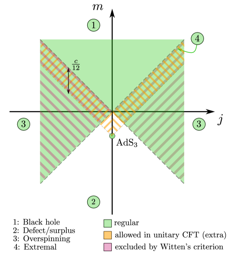
Figure 1: A summary of our analysis. The regular geometries (in green) comprise black holes (region 1), overspinning (region 3) and pure AdS₃ out of the conical geometries of region 2. Of these, the admissibility criterion of Witten:2021nzp excludes region 3, leaving only black holes and AdS₃. The orange region spans additional states allowed by unitarity in a dual conformal field theory.

Motivated by these considerations, in this note we will consider the family of complex metrics which arise from analytically continuing the BTZ-type metrics Banados:1992wn in the entire $(M,J)$ plane to imaginary time. We study which of these ‘quasi-Euclidean’ metrics qualify as saddle points for the grand canonical path integral, in the sense they are both smooth as well as obey Witten’s admissibility criterion. The result of this analysis is illustrated in Figure 1. Our main observation is that, while smoothness alone allows for the global AdS and BTZ black hole saddles as well as the overspinning solutions, the latter are in fact not admissible. Admissibility therefore successfully excises these metrics, in agreement with the Euclidean approach, where overspinning geometries do not contribute to the partition function.

2 BTZ class of metrics

The BTZ metric Banados:1992wn is the most general stationary, axisymmetric solution of the $(2+1)$-dimensional Einstein equations with negative cosmological constant, describing an object of arbitrary mass $M$ and angular momentum $J$. We will work in the conventions of Banados:1992gq and in units where the AdS radius is set to one, $l_{AdS}=1$. It is useful to define a dimensionless reduced mass and angular momentum

$$m=8G_{N}M,\qquad j=8G_{N}J.$$ (1)

The BTZ metric then takes the form

$$ds^{2}=-(r^{2}-m)dt^{2}+{r^{2}dr^{2}\over r^{4}-mr^{2}+{j^{2}\over 4}}+jdtd\tilde{\phi}+r^{2}d\tilde{\phi}^{2},$$ (2)

where $\tilde{\phi}$ has period $2\pi$. Global AdS₃ corresponds to $m=-1,j=0$. We will consider the class of metrics (2) for arbitrary real values of the parameters $m$ and $j$.

For later reference, it is useful to introduce the roots $r_{\pm}$ of the polynomial $x^{2}-mx+j^{2}/4$:

$$r_{\pm}=\pi\left(T_{+}\pm{\rm sgn}\,(m)T_{-}\right),$$ (3)

where we defined

$$T_{\pm}={1\over 2\pi}\sqrt{m\pm j}.$$ (4)

These generically complex parameters generalize the ‘left- and right-moving temperatures’ of the BTZ black hole. The sign in (3) was chosen such that

$${\rm Re\,}(r_{+}^{2})\geq{\rm Re\,}(r_{-}^{2})$$ (5)

for all values of $m$ and $j$.

We rewrite the metric (2) as

$$ds^{2} = -fdt^{2}+f^{-1}dr^{2}+r^{2}(d\phi+N^{\phi}dt)^{2},$$ (6)

$$f = r^{2}-m+{j^{2}\over 4r^{2}}={(r^{2}-r_{+}^{2})(r^{2}-r_{-}^{2})\over r^{2}},$$ (7)

$$N^{\phi} = {j\over 2r^{2}}-\Omega={r_{+}r_{-}\over r^{2}}-\Omega.$$ (8)

Here, we have also made an improper coordinate transformation $\tilde{\phi}=\phi-\Omega t$ which introduces an angular velocity at infinity,

$$ds^{2}\rightarrow-r^{2}dt^{2}+{dr^{2}\over r^{2}}+r^{2}\left(d(\phi-\Omega t)\right)^{2},$$ (9)

and describes AdS₃ in a rotating frame. Note that the Killing vector ${\partial_{t}}|_{\phi,r}$ is timelike at infinity only if the angular velocity $\Omega$ satisfies

$$|\Omega|<1.$$ (10)

It’s convenient to divide the $m,j$ plane into 4 physically distinct regions, see Figure 1:

1. Black hole regime, where $m>0,\ m>|j|$. The parameters $T_{\pm}$ and $r_{\pm}$ are real and positive, and $r_{+}$ and $r_{-}$ are the locations of the inner and outer horizons respectively.

2. Defect/surplus regime, where $m<0,\ |m|>|j|$. The parameters $T_{\pm}$ and $r_{\pm}$ are purely imaginary. This class includes the global AdS metric ($m=-1,j=0$), conical defects describing backreacted point particles Deser:1983nh ($-1<m<0,j=0$) and metrics with a conical surplus ($m<-1,j=0$), as well as spinning generalizations thereof.

3. Overspinning regime, where $|m|<|j|$. One of the ‘temperatures’ $T_{\pm}$ is real and the other is imaginary, while the $r_{\pm}^{2}$ are complex and each others conjugate.

4. Extremal regime, where $m=\pm j$. These metrics lie on the boundaries separating regions 1, 2 and 3 and include extremal spinning black holes for $m>0$, the zero-mass limit of the BTZ black hole for $m=0$, and extremal spinning defects for $m<0$.

The following table summarizes the values of the parameters in these regimes:

regime	$(m,j)$	$(T_{+},T_{-})$	$(r_{+},r_{-})$
1	$m>0,\ m>|j|$	$T_{\pm}>0$	$r_{+}>r_{-}\geq 0$
2	$m<0,\ |m|>|j|$	$T_{\pm}\in i\mathbb{R}$	$r_{\pm}\in i\mathbb{R},\ r_{-}^{2}<r_{+}^{2}\leq 0$
3	$|m|<|j|$	$T_{\pm}\in\mathbb{R},T_{\mp}\in i\mathbb{R}$	$r_{\pm}\in\mathbb{C},r_{+}^{2}=(r_{-}^{2})^{*}$
4	$m=\pm j$	$T_{\mp}=0,T_{\pm}={1\over\pi}\sqrt{m\over 2}$	$r_{+}^{2}=r_{-}^{2}={m\over 2}$

It is relevant to point out that in holographic theories the unitarity bound reads

$$m-|j|\geq-1.$$ (11)

Therefore, unitary holographic CFTs may in principle contain states in all four of the above regimes, as illustrated in Figure 1.

3 Quasi-Euclidean continuation

In the path-integral approach to quantum gravity Gibbons:1976ue , the grand canonical partition function at inverse temperature $\beta$ and angular potential $\Omega,$ (with $|\Omega|<1$) is expressed as a path integral over metrics,

$$Z(\beta,\Omega)={\rm tr}e^{-\beta(H+\Omega J)}\sim\int[Dg]e^{iS[g]},$$ (12)

where the metrics should behave near infinity as

$$ds^{2}\rightarrow r^{2}d\tau^{2}+{dr^{2}\over r^{2}}+r^{2}\left(d\phi-i\Omega d\tau\right)^{2}$$ (13)

with coordinates having the periods

$$(\tau,\phi)\sim(\tau+\beta,\phi)\sim(\tau,\phi+2\pi).$$ (14)

The asymptotic condition shows that the metrics included in the measure should be allowed to be complex. However, including all complex metrics does not lead to sensible results. Witten’s admissibility criterion Witten:2021nzp , which we review in Section 5, is a proposal to restrict to a subclass of physically sensible complex metrics.

In the semiclassical limit $G_{N}\rightarrow 0$, the path integral will be dominated by classical saddle points. A large class of potential classical saddles satisfying (13) is obtained from the metric (6) by continuing the time coordinate to the imaginary axis, $t\rightarrow i\tau$. The resulting metric is said to be quasi-Euclidean (qE) and takes the form

$$ds^{2}_{qE}=fd\tau^{2}+f^{-1}dr^{2}+r^{2}\left(d\phi+iN^{\phi}d\tau\right)^{2}.$$ (15)

Note that, as emphasized in the Introduction, in this approach one does not continue the parameters $j$ and $\Omega$ to imaginary values, which would result in a real Euclidean metric.

The metrics (15) generically have coordinate singularities where the metric degenerates. As in (pseudo-)Riemannian geometry, these can be either an artifact of the coordinate system (and disappear upon making a suitable coordinate change), or reflect a genuine pathology. We will interpret the latter case as a sign that the classical gravity approximation breaks down and we should not include the solution as a saddle.

Our strategy will be to first determine the qE metrics which are smooth and subsequently, in Section 5, analyze which ones obey Witten’s admissibility criterion.

4 Smoothness

In order to analyze the smoothness of the quasi-Euclidean metrics, it is useful to make a further coordinate redefinition. In the above coordinate system, the quasi-Euclidean (qE) metric (15) degenerates at $r=0$, where $\det g$ vanishes. Unless $r_{+}$ or $r_{-}$ also vanishes, this is a coordinate singularity which can be removed by defining the new coordinate

$$u=r^{2}.$$ (16)

The qE metric then becomes

$$ds^{2}_{qE}={(u-r_{+}^{2})(u-r_{-}^{2})\over u}d\tau^{2}+{du^{2}\over 4(u-r_{+}^{2})(u-r_{-}^{2})}+u\left(d\phi+i\left({r_{+}r_{-}\over u}-\Omega\right)d\tau\right)^{2}.\\$$ (17)

Coordinate singularities still occur when $u=r_{+}^{2}$ and $u=r_{-}^{2}$, while $\det g$ is constant for all values of $u$. This of course happens only if $r_{+}^{2}$ and $r_{-}^{2}$ are real, i.e. in the regimes 1, 2 and 4, while the overspinning regime 3 is free of coordinate singularities. When $r_{+}^{2}$ and $r_{-}^{2}$ are real it will be useful to divide the spacetime into subregions to the left (L), in the middle (M) and to the right (R) of the coordinate singularities:

$$L : \qquad u\leq r_{-}^{2},$$ (18)

$$M : \qquad r_{-}^{2}<u<r_{+}^{2},$$ (19)

$$R : \qquad r_{+}^{2}\leq u.$$ (20)

We note that in the extremal regime 4 the middle (M) region is absent.

In the rest of this section we want to establish in which regions and for which values of the parameters $\beta,\Omega$ the qE metrics (17) are invertible and smooth. In three-dimensional gravity, all curvature invariants are locally constant and detecting singularities is more subtle than in higher dimensions, requiring a careful description of the global manifold structure. Extending the Lorentzian analysis Banados:1992gq ; Cangemi:1992my , we will use the fact that the ‘quasi-Euclidean manifold’ on which the qE metric is defined can be obtained from the smooth group manifold $SL(2,\mathbb{C})$ by two operations: a quotient by a discrete group and a subsequent restriction to a three-dimensional real subspace. In sections 4.1 and 4.2 we establish when these operations introduce singularities. A complementary approach, presented in Section 4.3, is to study the holonomy of the Chern-Simons connections, which for regular solutions should be trivial when evaluated on smoothly contractible cycles. This will lead to results consistent with the first approach, though is somewhat more crude since, as we shall see, certain singularities in the manifold structure can still lead to trivial Chern-Simons holonomy.

4.1 The quotient

The $SL(2,\mathbb{C})$ group manifold can be viewed as a smooth hypersurface in $\mathbb{C}^{4}$,

$$\det G=G_{11}G_{22}-G_{12}G_{21}=1,$$ (21)

with invariant metric

$$ds^{2}=-{1\over 2}\,{\rm tr}\left(dG^{-1}dG\right)=-dG_{11}dG_{22}+dG_{12}dG_{21}.$$ (22)

When $m>0$, the aforementioned quotient amounts to imposing the following two identifications:

$$I_{1}:\qquad(G_{11},G_{22},G_{12},G_{21}) \sim (e^{2\pi r_{+}}G_{11},e^{-2\pi r_{+}}G_{22},e^{-2\pi r_{-}}G_{12},e^{2\pi r_{-}}G_{21})$$

$${}I_{2}:\qquad(G_{11},G_{22},G_{12},G_{21}) \sim (e^{i(r_{-}-\Omega r_{+})\beta}G_{11},e^{-i(r_{-}-\Omega r_{+})\beta}G_{22},$$ (23)

$$e^{-i(r_{+}-\Omega r_{-})\beta}G_{12},e^{i(r_{+}-\Omega r_{-})\beta}G_{21}),$$

while for $m<0$, one has to interchange $r_{+}$ and $r_{-}$ in these expressions. Note that these identifications preserve the hypersurface (21). Their appropriateness will become manifest in Section 4.2, where we will recover the qE metric (17) by selecting a real slice of a group element satisfying (23). We should also note that (23) breaks down in the limit of extremal metrics, i.e. regime 4, the details of which are discussed in Appendix A.

The quotient space is a smooth manifold only if the identifications act without fixed points on the hypersurface (21), see e.g. HawkingEllis . Both identifications have a fixed point in $\mathbb{C}^{4}$ at $G_{11}=G_{22}=G_{12}=G_{21}=0$, which however does not lie on (21). From the form of (23) we see that singularities can occur on two possible loci, namely

• at $G_{12}=G_{21}=0$, $G_{11}G_{22}=1$. This is a fixed locus of $I_{1}$ for $r_{+}=0$ provided that $r_{-}\neq i$. The case $r_{+}=0$, $r_{-}=i$, is special, since $I_{1}$ then becomes trivial. Similarly, it is a fixed locus of $I_{2}$ for $\Omega={r_{-}\over r_{+}}$ provided that $\beta\neq{2\pi r_{+}\over r_{+}^{2}-r_{-}^{2}}$, with the case $\Omega={r_{-}\over r_{+}}$, $\beta={2\pi r_{+}\over r_{+}^{2}-r_{-}^{2}}$ corresponding to $I_{2}$ becoming trivial.

• at $G_{11}=G_{22}=0$, $G_{12}G_{21}=-1$. This is a fixed locus of $I_{1}$ for $r_{-}=0$ and $r_{+}\neq i$, and a fixed locus of $I_{2}$ for $\Omega={r_{-}\over r_{+}}$ and $\beta\neq{2\pi r_{+}\over r_{+}^{2}-r_{-}^{2}}$.

As one would expect, these loci correspond to the coordinate singularities at $u=r_{+}^{2}$ or $u=r_{-}^{2}$ as we shall see shortly. Recalling the ranges of the parameters $r_{\pm}$ in the various regimes and the fact that $\beta$ and $\Omega$ are required to be real, the above analysis (and its extension to region 4 in Appendix A) can be summarized in the following table of regular quotients:

regime	quotient regular for
1	$\left\{\begin{array}[]{l}\Omega={r_{-}\over r_{+}},\beta={2\pi r_{+}\over r_{+}^{2}-r_{-}^{2}}\\ \Omega={r_{+}\over r_{-}},\beta={2\pi r_{-}\over r_{+}^{2}-r_{-}^{2}}\\ \Omega\neq\{{r_{-}\over r_{+}},{r_{+}\over r_{-}}\}\end{array}\right.$
2	$\left\{\begin{array}[]{l}r_{-}=i,r_{+}=0\\ \Omega\neq\{{r_{-}\over r_{+}},{r_{+}\over r_{-}}\}\end{array}\right.$
3	always
4	$\left\{\begin{array}[]{l}\Omega={\rm sgn}\,{m\over j},\beta=\infty,m>0\\ \Omega\neq{\rm sgn}\,{m\over j},m\neq 0\end{array}\right.$

Table 1: Summary of smooth quotients.

A remark is in order concerning this table. In principle, we could have also allowed the values of $\beta$ in the first and second lines and of $r_{-}$ in the fourth line to be an integer multiple of the displayed values, since the relevant identification would then still act trivially. However, in doing so we would no longer describe a quotient of $SL(2,\mathbb{C})$ but rather a multi-sheeted covering space. Furthermore, the resulting manifold would not be a smooth covering space (see e.g. Lee ), since the sheets would meet at the loci described above, and therefore we will not consider these spacetimes in this context.

4.2 The real slice

Now we turn to the second operation of restricting the above quotients to a real, three-dimensional subspace. For this purpose we parametrize the group element as

$$G_{11} = z_{1}w\exp\left({r_{+}\phi}+i(r_{-}-\Omega r_{+})\tau\right)$$

$${}G_{22} = z_{1}w^{-1}\exp\left[-\left({r_{+}\phi}+i(r_{-}-\Omega r_{+})\tau\right)\right]$$

$${}G_{12} = z_{2}w^{-1}\exp\left[-\left({r_{-}\phi}+i(r_{+}-\Omega r_{-})\tau\right)\right]$$

$${}G_{21} = z_{2}w\exp\left({r_{-}\phi}+i(r_{+}-\Omega r_{-})\tau\right),$$ (24)

where $z_{1},z_{2}\in\mathbb{C},w\in\mathbb{C}\backslash\{0\}$ and $\phi,\tau\in\mathbb{R}$. For instance, in regime 1 one checks that these are good coordinates away from the locus where at least one of the $G_{ij}$ vanishes, as long as $r_{+}\neq r_{-}$ and $\Omega\neq-1$. The equation (21) becomes

$$z_{1}^{2}-z_{2}^{2}=1,$$ (25)

while the identifications (23) read

$$I_{1}:\phi\sim\phi+2\pi,\qquad I_{2}:\tau\sim\tau+\beta.$$ (26)

Regime 1

Let us discuss the real slice in terms of these coordinates firstly in regime 1. The qE geometry in the subregions 1R, 1M, and 1L arises from imposing:

• Region 1R: $w=1,\arg z_{1}=\arg z_{2}=0.$

• Region 1M: $w=1,\arg z_{1}=0,\arg z_{2}={\pi\over 2}.$

• Region 1L: $w=1,\arg z_{1}=\arg z_{2}={\pi\over 2}.$

In all cases, $z_{1}$ and $z_{2}$ can be expressed in terms of the real coordinate $u$ as

$$z_{1}=\sqrt{u-r_{-}^{2}\over r_{+}^{2}-r_{-}^{2}},\qquad z_{2}=\sqrt{u-r_{+}^{2}\over r_{+}^{2}-r_{-}^{2}}.$$ (27)

One checks that the pullback of the invariant metric (22) is indeed (17).

Let us now discuss in which cases the pullback to the real slice of the smooth metric on the regular quotient spaces listed in Table 1 fails to be a smooth complex metric. For $\Omega={r_{-}\over r_{+}}$ and $\beta={2\pi r_{+}\over r_{+}^{2}-r_{-}^{2}}$, the locus $u\rightarrow r_{+}^{2}$ has codimension 2 and is the $\phi$-circle embedded as $G_{12}=G_{21}=0,G_{11}=G_{22}^{-1}=e^{r_{+}\phi}$. In other words, the $\tau$-circle ‘pinches off’ there. From the form of $G_{12},G_{21}$ we see that it does so smoothly and that the spacetime locally looks like $\mathbb{R}^{2}\times S^{1}$. In this case the region 1R ends smoothly at $u\rightarrow r_{+}^{2}$. Similarly, for $\Omega={r_{+}\over r_{-}}$ and $\beta={2\pi r_{-}\over r_{+}^{2}-r_{-}^{2}}$ the region 1L forms a smooth submanifold.

For $\Omega\neq{r_{-}\over r_{+}}$, the locus $u=r_{+}^{2}$ has codimension 1: it is an $S^{1}\times S^{1}$ embedded as

$$G_{12}=G_{21}=0,\qquad G_{11}=G_{22}^{-1}=e^{r_{+}\phi+2\pi i(r_{-}-\Omega r_{+})\tau}.$$ (28)

Neither the $\tau$ or $\phi$-circles pinch off and one expects the spacetime to continue into region 1M. However, the regions 1R and 1M cannot be joined together smoothly as we shall now argue in two complimentary ways: the first based on degeneracy of the pulled-back metric and the second from the fact that the embedded real submanifold is not sufficiently smooth.

Firstly, one can argue that the coordinate singularity in $u=r_{+}^{2}$ is not removable. Indeed, from (28) we see that $\partial_{\phi}$ and $\partial_{\tau}$ provide linearly independent basis vectors of the tangent space at each point. The metric on this locus is however always of rank one, independent of the chosen coordinates on the real slice. Indeed, the metric (22) pulled back to the $u=r_{+}^{2}$ locus $G_{12}=G_{21}=0,G_{11}=G_{22}^{-1}$ is

$$ds^{2}_{hor}={dG_{11}^{2}\over G_{11}}.$$ (29)

Since a nondegenerate metric should have maximal rank when pulled back to a proper submanifold, we see that the quasi-Euclidean ‘metric’ is in this case degenerate.

A second argument comes from considering the smoothness of the 3D submanifold. It is instructive to see how the radial coordinate lines of constant $\phi$ and $\tau$ are embedded in the ambient space in the vicinity of $u=r_{+}^{2}$. While they are embedded as straight lines in the $G_{11}$ and $G_{22}$ planes, they are not embedded as differentiable curves in the $G_{12}$ and $G_{21}$ planes, where they have a rectangular ‘corner’ as shown in Figure 2(a).

Figure 2: Radial coordinate lines embedded in the $G_{12}$ plane in (a) Region 1 for $\Omega\neq{r_{-}\over r_{+}}$ (b) Region 3.

Therefore, the radial coordinate lines and the embedded 3D real manifold are at most of class ${\cal C}^{0}$ (see HawkingEllis ). However, in order to be able to reliably compute the curvature of the pulled-back metric, one would need the embedding map to be at least of class ${\cal C}^{2}$. Similarly, one argues that, for $\Omega\neq{r_{+}\over r_{-}}$, the region 1L cannot be not smoothly joined to the region 1M at $u=r_{-}^{2}$.

Regime 2

In region 2, the real slice in subregions 2R, 2M, and 2L is:

• Region 2R: $w=1,\arg z_{1}=\arg z_{2}=0.$

• Region 2M: $w=1,\arg z_{1}={\pi\over 2},\arg z_{2}=0.$

• Region 2L: $w=1,\arg z_{1}=\arg z_{2}={\pi\over 2}.$

In all cases, $z_{1}$ and $z_{2}$ can be expressed in terms of the real coordinate $u$ as

$$z_{1}=\sqrt{u-r_{+}^{2}\over r_{+}^{2}-r_{-}^{2}},\qquad z_{2}=\sqrt{u-r_{-}^{2}\over r_{+}^{2}-r_{-}^{2}}.$$ (30)

Similarly as in regime 1, one argues that for $r_{-}=i,r_{+}=0$, the region $2R$ is a smooth submanifold which ends at $u=0$, where the $\phi$-circle pinches off smoothly. Also, as above one shows that for $r_{-}=i,r_{+}=0$, the regions 2L and 2M cannot join smoothly. Similarly, when $\Omega\neq{r_{-}\over r_{+}},r_{+}\neq 0$, the region 2R cannot be smoothly joined to the region 2M.

Regime 3

In the overspinning regime, the real slice is defined by setting

$$w=1,\qquad z_{1}=\sqrt{u-r_{-}^{2}\over r_{+}^{2}-r_{-}^{2}},\qquad z_{2}=\sqrt{u-r_{+}^{2}\over r_{+}^{2}-r_{-}^{2}}.$$ (31)

As already mentioned, the metric is everywhere nondegenerate and one checks that (31) defines a smooth submanifold; for example, the radial curves are now smooth curves in the ambient $\mathbb{C}^{4}$ as illustrated in Figure 2(b).

Regime 4

Using the embedding (56) in Appendix A, one can similarly show that the real slice defining the extremal metrics is not smooth for $\Omega\neq{\rm sgn}\,{m\over j}$, $m\neq 0$. Smooth extremal metrics can be thought of as $j\rightarrow\pm m$ limits of the smooth metrics in region 1, in the sense of requiring $\beta\rightarrow\infty,\Omega\rightarrow\pm 1$ while keeping $\beta(1-\Omega^{2})={4\pi\over m}$ fixed.

Combining the above results, we arrive at Table 2 of smooth qE metrics. We also indicate in the last column whether the spacetime is a potential saddle for the partition function $Z(\beta,\Omega)$ in (12). For this it needs to contain the region $u\rightarrow\infty$ and satisfy $|\Omega|<1$.

region	regular if	potential saddle?
1R	$\beta={2\pi r_{+}\over r_{+}^{2}-r_{-}^{2}},\Omega={r_{-}\over r_{+}}$	$\times$
1L	$r_{-}\neq 0,\beta={2\pi r_{-}\over r_{+}^{2}-r_{-}^{2}},\Omega={r_{+}\over r_{-}}$	-
2R	$r_{+}=0,r_{-}=i,\beta\in\mathbb{R},$	$\times$
3	$\beta,\Omega\in\mathbb{R}$	$\times$
4L	$\beta\rightarrow\infty,\Omega\rightarrow{\rm sgn}{j\over m}$	-
4R	$\beta\rightarrow\infty,\Omega\rightarrow{\rm sgn}{j\over m}$	$\times$

Table 2: Summary of smooth qE metrics.

4.3 Smoothness and holonomies

In order to complement the above discussion on regularity, one can study holonomies of the Chern-Simons connections associated to the metric Cangemi:1992my . These quantities encode information on the topology of spacetime, but they can still fail to detect certain singularities. Despite these shortcomings, one can at least compute the relevant holonomies as a consistency check.

The flat $SL(2,\mathbb{C})\times SL(2,\mathbb{C})$ gauge potentials describing the quasi-Euclidean metrics (17) are of the form

$$A=g^{-1}dg,\qquad\tilde{A}=\tilde{g}^{-1}d\tilde{g}.$$ (32)

The $SL(2,\mathbb{C})$ group elements can be can be obtained from the group element $G$ by writing it as

$$G=g\tilde{g}^{-1},\qquad g=e^{\pi T_{-}\left(\phi-i(1+\Omega)\tau\right)\sigma_{3}}B(u),\qquad\tilde{g}=e^{-\pi T_{+}\left(\phi+i(1-\Omega)\tau\right)\sigma_{3}}B(u)^{-1},$$ (33)

where the specific form of the $2\times 2$ matrix $B(u)$ is not needed, since we shall seek trivial holonomies around curves with constant $u_{0}$.

Using (33) one can easily compute the holonomies of $A$ and $\tilde{A}$ around closed curves $\gamma$ at constant radius $u=u_{0}$. For an angular circle of period $2\pi$ at constant $\tau=\tau_{0}$ one finds

$$H_{\gamma} = B(u_{0})^{-1}e^{2\pi^{2}T_{-}\sigma_{3}}B(u_{0})\,$$ (34)

$$\tilde{H}_{\gamma} = B(u_{0})e^{-2\pi^{2}T_{+}\sigma_{3}}B(u_{0})^{-1}\,.$$ (35)

These are trivial (meaning equal to $1$ or $-1$, i.e. in the center of $SL(2,\mathbb{C})$) for $r_{\pm}\in i\mathbb{Z}$, namely for

$$m=-{p^{2}+q^{2}\over 2},\qquad j=-{p^{2}-q^{2}\over 2},$$ (36)

where $p,q$ are nonzero integers. In the extremal case, when either of them vanishes, one needs to use a different group element. We discuss this subtlety in Appendix A. Except for the pure AdS₃ case $p=q=1$, these represent a discrete family of conical surpluses and their spinning generalizations. Such branched covering spaces are singular as manifolds as we have explained below Table 1. In region 1 (black hole regime) the angular circle is not contractible, so there is no issue.

For a time circle with period $\beta$ at constant $\phi=\phi_{0}$, the holonomies read

$$H_{\gamma} = B(u_{0})^{-1}e^{-i\pi T_{-}(1+\Omega)\beta\sigma_{3}}B(u_{0})\,,$$ (37)

$$\tilde{H}_{\gamma} = B(u_{0})e^{-i\pi T_{+}(1-\Omega)\beta\sigma_{3}}B(u_{0})^{-1}\,,$$ (38)

which are in the center only for

$$\beta = \pi\,\frac{p(r_{+}+r_{-})+q(r_{+}-r_{-})}{r_{+}^{2}-r_{-}^{2}}\,,$$ (39)

$$\Omega = \frac{p(r_{+}+r_{-})-q(r_{+}-r_{-})}{p(r_{+}+r_{-})+q(r_{+}-r_{-})}$$ (40)

with $p\,,\,q\in\mathbb{Z}$. However, most of these solutions again describe singular branched covering spaces. The inequivalent “minimal” choices are (representable by) $p=q=1$ and $p=-q=1$. In region 1 the former is consistent with the regularity conditions of the black hole geometry (region 1R), while the latter gives region 1L which is not a potential saddle for the partition function.

In region 2, these solutions would lead to imaginary $\beta$ which gives a singular geometry. A similar argument excludes region 3. All in all, the regular geometries that we have determined do have trivial Chern-Simons holonomies along contractible curves, as expected, but this condition by itself is not sufficient.

5 Admissibility

In this section we investigate in which regions the qE metrics (17) obey Witten’s admissibility criterion. As discussed in Kontsevich:2021dmb ; Witten:2021nzp , defining a well-behaved (semiclassical) path integral on a manifold requires that large field fluctuations be suppressed by the (exponential of the) Euclidean action. For complex metrics coupled to $p$-form fields, the real part of the action ought to be positive definite, or more generally bounded from below. Extending this criterion to fields of different type is more subtle, due to the difficulties in coupling them consistently to gravity.

In 3 dimensions, the admissibility conditions reduce to Witten:2021nzp

$${\rm Re\,}(\sqrt{g})>0,\qquad{\rm Re\,}(\sqrt{g}\lambda_{i}^{-1})>0,$$ (41)

where $\lambda_{i},i=1,2,3$ are the eigenvalues of the metric. Applying to (17), the first condition is satisfied since $\sqrt{g}={1\over 2}$. The remaining conditions reduce to the requirement that $g_{uu}>0$ and that the eigenvalues of the 2D $\tau,\phi$ submatrix have positive real parts. As shown in Witten:2021nzp , this latter condition is equivalent to $g_{\tau\tau}>0$. Using (17), the admissibility criteria $g_{uu}>0$, $g_{\tau\tau}>0$ then reduce to

$$I: (u-r_{+}^{2})(u-r_{-}^{2}) >0,$$ (42)

$$II: (1-\Omega^{2})u-(r_{+}^{2}+r_{-}^{2})+2r_{+}r_{-}\Omega >0.$$ (43)

The second condition, which is linear in $u$, is always satisfied on a half-infinite line in the $u$ coordinate and can be rephrased as

$$II: \left\{\begin{array}[]{ll}u>u_{0}&{\rm for\ }|\Omega|<1\\ (r_{+}\mp r_{-})^{2}<0&{\rm for\ }\Omega=\pm 1\\ u<u_{0}&{\rm for\ }|\Omega|>1\end{array}\right.,$$ (47)

where $u_{0}$ is the zero of $g_{\tau\tau}$, namely

$$u_{0}={r_{+}^{2}+r_{-}^{2}-2r_{+}r_{-}\Omega\over 1-\Omega^{2}}.$$ (48)

We now investigate in which of the regions described above, i.e. (1L, 1M, 1R; 2L, 2M, 2R; 3; 4L, 4R), the conditions $I$ and $II$ are satisfied, possibly upon imposing some restriction on the angular velocity $\Omega$. In regions 1M, 2M the condition $I$ is violated. In region 1L one finds that $I$ and $II$ hold simultaneously only if $u_{0}=r_{-}^{2}$ and $|\Omega|<1$, while in region 1R they hold if $u_{0}=r_{+}^{2}$ and $|\Omega|>1$. In region 2L, conditions $I$ and $II$ both hold for any $|\Omega|>1$, while in region 2R they hold for $|\Omega|<1$. In region 3, condition $II$ is always violated in some range of $u$ (namely $u<u_{0}$ when $|\Omega|<1$ and $u>u_{0}$ when $|\Omega|>1$). In region 4, taking $m=j$ for definiteness, condition I is obeyed (except at $u=m/2$). When $\Omega<1$, condition II is violated in region 4R for ${m\over 2}<u<{m\over\Omega+1}$, while for $\Omega>1$, it is violated in region 4L for ${m\over\Omega+1}<u<{m\over 2}$. Thefore both 4L and 4R become admissible in the limit $\Omega\rightarrow 1$. These conclusions are summarized in the following table:

region	admissible if
1L	$\Omega={r_{+}\over r_{-}}$
1M	never
1R	$\Omega={r_{-}\over r_{+}}$
2L	$|\Omega|>1$
2M	never
2R	$|\Omega|<1$
3	never
4L	$\Omega\rightarrow{\rm sgn}\,{j\over m}$
4R	$\Omega\rightarrow{\rm sgn}\,{j\over m}$

Table 3: Summary of admissible qE metrics.

6 Discussion

Combining the results from the smoothness (Table 2) and admissibility (Table 3) analyses, we conclude that the smooth, admissible quasi-Euclidean saddles contributing to the partition function (12) are

region	smooth & admissible for
1R	$\beta={2\pi r_{+}\over r_{+}^{2}-r_{-}^{2}},\Omega={r_{-}\over r_{+}}$
2R	$r_{+}=0,r_{-}=i,\beta\in\mathbb{R},|\Omega|<1,$

In other words, the contributing saddles are the black holes with the standard relations between $\beta,\Omega$ and $m,j$, and rotating thermal AdS. Therefore the admissible complex saddles agree with those considered in the more standard approach of going to Euclidean signature by continuing also the angular momentum and the angular potential to imaginary values Maldacena:1998bw . For this agreement it was crucial that admissibility discards the overspinning metrics. These would be hard to interpret thermodynamically as they are wormhole-like geometries connecting two asymptotic regions, and do not contribute in the Euclidean approach. We see it as an encouraging sign that the method passes this nontrivial consistency check.

The computation of the contribution of these saddles to the partition function (12) proceeds in the standard manner using holographic renormalization Henningson:1998gx ; Balasubramanian:1999re . The regularized on-shell action is

$$S_{reg}={1\over 4\pi G_{N}}\left[\int_{u\leq L^{2}}d^{3}x\sqrt{-g}-{1\over 2}\int_{u=L^{2}}d^{2}x\sqrt{-\gamma}(K-1)\right],$$ (49)

where $L$ is a large radius cutoff, to be taken to infinity in the end. Evaluating on a solution, the divergent terms of order $L^{2}$ are cancelled and taking $L$ to infinity the result is

$$iS_{ren}={c\over 12}\beta(2u_{0}-m).$$ (50)

Here, $c={3\over 2G_{N}}$ and $u_{0}$ is the starting point of the radial interval $u_{0}\leq u\leq L^{2}$. For both saddles, the starting point is at $u_{0}=r_{+}^{2}$, leading to

$$Z(\beta,\Omega) = e^{iS_{ren,1R}}+e^{iS_{ren,2R}}=e^{{c\over 3}{\pi^{2}\over\beta(1-\Omega^{2})}}+e^{{c\over 12}\beta}.$$ (51)

The Hawking-Page transition Hawking:1982dh arises from exchange of dominance between these saddles in $(\beta,\Omega)$ space (see also Kurita:2004yn ).

Appendix A Details of the extremal case

Now let us consider the extremal metrics where $m=\pm j$. Without loss of generality (by making a parity transformation if necessary), we can assume that

$$m=j$$ (52)

so that

$$T_{-}=0,\qquad T_{+}={r_{+}\over\pi}={1\over\pi}\sqrt{m\over 2}.$$ (53)

In this case, it turns out that the identifications act on the complex $2\times 2$ group element $G$ as follows:

$$I_{1}:\qquad G \sim e^{\sqrt{2}\pi\sigma_{+}}Ge^{\sqrt{2}\pi(\sigma_{-}+m\sigma_{+})},$$ (54)

$$I_{2}:\qquad G \sim e^{-{i\over\sqrt{2}}(1+\Omega)\beta\sigma_{+}}Ge^{{i\over\sqrt{2}}(1-\Omega)\beta(\sigma_{-}+m\sigma_{+})},$$ (55)

where $\sigma_{\pm}={1\over 2}(\sigma_{1}\pm i\sigma_{2})$. Aside from $G=0$, these have the following fixed points. $I_{1}$ has fixed points only when $m=0$, namely at $G_{21}=-G_{12},G_{22}=0$. The identification $I_{2}$ has fixed loci for $\Omega=1$, namely at $G_{21}=G_{22}=0$ and for $m=0$ at $G_{21}={{1+\Omega\over 1-\Omega}}G_{21}$. This leads to the smooth quotient spaces given in Table 1.

The real slice is in this case defined by taking the group element to be of the form

$$G=\exp{\left(\phi-i(1+\Omega)\tau\right){\sigma_{+}}\over\sqrt{2}}\left(\begin{array}[]{cc}{1\over\sqrt{a}}&0\\ 0&\sqrt{a}\end{array}\right)\exp{\left(\phi+i(1-\Omega)\tau\right)\left(\sigma_{-}+m\sigma_{+}\right)\over\sqrt{2}},$$ (56)

where

$$a=2u-m=2(u-r_{+}^{2}).$$ (57)

One sees from (56) that in this case the horizon $u\rightarrow r_{+}^{2}$ corresponds points at infinity in $SL(2,\mathbb{C})$:

$$G_{11}\rightarrow\infty,\quad G_{22}\rightarrow 0,\quad G_{12}\rightarrow\infty,\quad G_{21}\rightarrow 0.$$ (58)

References

- (1) G. W. Gibbons and S. W. Hawking, “Action Integrals and Partition Functions in Quantum Gravity,” Phys. Rev. D 15 (1977) 2752–2756.
- (2) E. Witten, “A Note On Complex Spacetime Metrics,” arXiv:2111.06514 [hep-th].
- (3) M. Kontsevich and G. Segal, “Wick Rotation and the Positivity of Energy in Quantum Field Theory,” Quart. J. Math. Oxford Ser. 72 no. 1-2, (2021) 673–699, arXiv:2105.10161 [hep-th].
- (4) J. Louko and R. D. Sorkin, “Complex actions in two-dimensional topology change,” Class. Quant. Grav. 14 (1997) 179–204, arXiv:gr-qc/9511023.
- (5) O. Aharony, F. Benini, O. Mamroud, and E. Milan, “A gravity interpretation for the Bethe Ansatz expansion of the SYM index,” Phys. Rev. D 104 (2021) 086026, arXiv:2104.13932 [hep-th].
- (6) S. Bondarenko, “Dynamical Signature: Complex Manifolds, Gauge Fields and Non-Flat Tangent Space,” Universe 8 no. 10, (2022) 497, arXiv:2111.06095 [gr-qc].
- (7) J.-L. Lehners, “Allowable complex metrics in minisuperspace quantum cosmology,” Phys. Rev. D 105 no. 2, (2022) 026022, arXiv:2111.07816 [hep-th].
- (8) M. Visser, “Feynman’s i prescription, almost real spacetimes, and acceptable complex spacetimes,” JHEP 08 (2022) 129, arXiv:2111.14016 [gr-qc].
- (9) G. J. Loges, G. Shiu, and N. Sudhir, “Complex saddles and Euclidean wormholes in the Lorentzian path integral,” JHEP 08 (2022) 064, arXiv:2203.01956 [hep-th].
- (10) C. Jonas, J.-L. Lehners, and J. Quintin, “Uses of complex metrics in cosmology,” JHEP 08 (2022) 284, arXiv:2205.15332 [hep-th].
- (11) F. Briscese, “Note on complex metrics, complex time, and periodic universes,” Phys. Rev. D 105 no. 12, (2022) 126028, arXiv:2206.09767 [hep-th].
- (12) G. Araujo-Regado, “Holographic Cosmology on Closed Slices in 2+1 Dimensions,” arXiv:2212.03219 [hep-th].
- (13) O. Hulik, J. Raeymaekers, and O. Vasilakis, “Information recovery from pure state geometries in 3D,” JHEP 06 (2020) 119, arXiv:1911.12309 [hep-th].
- (14) S. W. Hawking and D. N. Page, “Thermodynamics of Black Holes in anti-De Sitter Space,” Commun. Math. Phys. 87 (1983) 577.
- (15) M. Banados, C. Teitelboim, and J. Zanelli, “The Black hole in three-dimensional space-time,” Phys. Rev. Lett. 69 (1992) 1849–1851, arXiv:hep-th/9204099.
- (16) M. Banados, M. Henneaux, C. Teitelboim, and J. Zanelli, “Geometry of the (2+1) black hole,” Phys. Rev. D 48 (1993) 1506–1525, arXiv:gr-qc/9302012. [Erratum: Phys.Rev.D 88, 069902 (2013)].
- (17) S. Carlip and C. Teitelboim, “Aspects of black hole quantum mechanics and thermodynamics in (2+1)-dimensions,” Phys. Rev. D 51 (1995) 622–631, arXiv:gr-qc/9405070.
- (18) O. Miskovic and J. Zanelli, “On the negative spectrum of the 2+1 black hole,” Phys. Rev. D 79 (2009) 105011, arXiv:0904.0475 [hep-th].
- (19) M. Briceño, C. Martínez, and J. Zanelli, “Overspinning naked singularities in AdS3 spacetime,” Phys. Rev. D 104 no. 4, (2021) 044023, arXiv:2105.06488 [gr-qc].
- (20) S. Deser and R. Jackiw, “Three-Dimensional Cosmological Gravity: Dynamics of Constant Curvature,” Annals Phys. 153 (1984) 405–416.
- (21) D. Cangemi, M. Leblanc, and R. B. Mann, “Gauge formulation of the spinning black hole in (2+1)-dimensional anti-De Sitter space,” Phys. Rev. D 48 (1993) 3606–3610, arXiv:gr-qc/9211013.
- (22) S. Hawking and G. Ellis, The large-scale structure of space-time. Cambridge University Press, 1973.
- (23) J. Lee, Introduction to Smooth Manifolds. Springer, 2012.
- (24) A. Castro, R. Gopakumar, M. Gutperle, and J. Raeymaekers, “Conical Defects in Higher Spin Theories,” JHEP 02 (2012) 096, arXiv:1111.3381 [hep-th].
- (25) E. Perlmutter, T. Prochazka, and J. Raeymaekers, “The semiclassical limit of CFTs and Vasiliev theory,” JHEP 05 (2013) 007, arXiv:1210.8452 [hep-th].
- (26) A. Campoleoni and S. Fredenhagen, “On the higher-spin charges of conical defects,” Phys. Lett. B 726 (2013) 387–389, arXiv:1307.3745 [hep-th].
- (27) J. Raeymaekers, “Quantization of conical spaces in 3D gravity,” JHEP 03 (2015) 060, arXiv:1412.0278 [hep-th].
- (28) H. Afshar, D. Grumiller, M. M. Sheikh-Jabbari, and H. Yavartanoo, “Horizon fluff, semi-classical black hole microstates — Log-corrections to BTZ entropy and black hole/particle correspondence,” JHEP 08 (2017) 087, arXiv:1705.06257 [hep-th].
- (29) J. M. Maldacena and A. Strominger, “AdS(3) black holes and a stringy exclusion principle,” JHEP 12 (1998) 005, arXiv:hep-th/9804085.
- (30) M. Henningson and K. Skenderis, “The Holographic Weyl anomaly,” JHEP 07 (1998) 023, arXiv:hep-th/9806087.
- (31) V. Balasubramanian and P. Kraus, “A Stress tensor for Anti-de Sitter gravity,” Commun. Math. Phys. 208 (1999) 413–428, arXiv:hep-th/9902121.
- (32) Y. Kurita and M.-a. Sakagami, “CFT description of three-dimensional Hawking Page transition,” Prog. Theor. Phys. 113 (2005) 1193–1213, arXiv:hep-th/0403091.