The DEHVILS Survey Overview and Initial Data Release: High-Quality Near-Infrared Type Ia Supernova Light Curves at Low Redshift

Abstract

While the sample of optical Type Ia Supernova (SN Ia) light curves (LCs) usable for cosmological parameter measurements surpasses 2000, the sample of published, cosmologically viable near-infrared (NIR) SN Ia LCs, which have been shown to be good “standard candles,” is still $\lesssim$ 200. Here, we present high-quality NIR LCs for 83 SNe Ia ranging from $0.002<z<0.09$ as a part of the Dark Energy, H₀, and peculiar Velocities using Infrared Light from Supernovae (DEHVILS) survey. Observations are taken using UKIRT’s WFCAM, where the median depth of the images is 20.7, 20.1, and 19.3 mag (Vega) for Y, J, and H-bands, respectively. The median number of epochs per SN Ia is 18 for all three bands (YJH) combined and 6 for each band individually. We fit 47 SN Ia LCs that pass strict quality cuts using three LC models, SALT3, SNooPy, and BayeSN and find scatter on the Hubble diagram to be comparable to or better than scatter from optical-only fits in the literature. Fitting NIR-only LCs, we obtain standard deviations ranging from 0.128–0.135 mag. Additionally, we present a refined calibration method for transforming 2MASS magnitudes to WFCAM magnitudes using HST CALSPEC stars that results in a 0.03 mag shift in the WFCAM Y-band magnitudes.

tablenum

1 Introduction

Table 1: Publicly available SN counts with NIR data after cumulative cuts

	Total	DEHVILS (% of Total)	CSP	CfA	RATIR	SweetSpot	RAISIN
Before Cuts	429	96 (22%)	120	94	41	33	45
Type Ia normala	368	83 (23%)	85	88	38	30	44
$\geq$ 3 NIR epochsb	345	83 (24%)	82	86	33	17	44
NIR near peakc	193	71 (37%)	48	49	21	4	0
$z_{\textrm{CMB}}>0.01$	171	67 (39%)	40	39	21	4	0

• Spectroscopically confirmed as Type Ia and designated as normal (e.g., exclusion of Iax, 86G-like, 91T-like, 91bg-like, 06gz-like, 06bt-like, Super-Chandrasekhar, and Ia’s interacting with circumstellar matter).

• Number of unique nights with a NIR observation.

• At least one NIR observation within $\pm 3$ days of fitted NIR maximum.

Type Ia Supernovae (SNe Ia) can be used to characterize the expansion of our universe (e.g., Freedman et al., 2019; Riess et al., 2022), and historically, SNe Ia have primarily been studied at optical wavelengths (e.g., Phillips, 1993; Hamuy et al., 1996; Riess et al., 1998, 1999; Perlmutter et al., 1999; Jha et al., 2006; Guy et al., 2010; Conley et al., 2011; Betoule et al., 2014; Jones et al., 2018; Scolnic et al., 2018; Brout et al., 2019, 2022). Analysis in the near-infrared (NIR) has advantages however — namely that SNe Ia in the NIR are more nearly standard candles as the SN light is less affected by dust and more uniform in luminosity (Meikle, 2000; Krisciunas et al., 2004; Wood-Vasey et al., 2008; Mandel et al., 2009; Folatelli et al., 2010; Phillips, 2012; Kattner et al., 2012; Barone-Nugent et al., 2012; Avelino et al., 2019; Mandel et al., 2022). But, observing and working with SNe Ia in the NIR is difficult. The sky background is much brighter in the NIR than in the optical, making NIR light from SNe more difficult to observe. Additionally, galaxies are brighter relative to SNe in the NIR, making light from SNe discovered on top of galaxy light more difficult to extract; SNe Ia are fainter in the NIR; and NIR detectors have historically trailed in both quantity and quality to optical detectors. Due to these difficulties, fewer SNe Ia have been observed in the NIR, and less work has been done in terms of NIR SN Ia testing, analyzing, and light curve (LC) modeling than in the optical.

NIR SN Ia samples and analyses have been performed by projects such as the Carnegie Supernova Project (CSP; Hamuy et al., 2006) through CSP-I (Contreras et al., 2010; Stritzinger et al., 2011; Krisciunas et al., 2017) and CSP-II (yet to be publicly available; Phillips et al., 2019; Hsiao et al., 2019), CfA (Wood-Vasey et al., 2008; Friedman et al., 2015), RATIR (Johansson et al., 2021), SweetSpot (Weyant et al., 2018), RAISIN (Jones et al., 2022), and are ongoing in the VISTA Extragalactic Infrared Legacy Survey (VEILS) and the Supernovae in the InfRAred Avec Hubble (SIRAH) projects. However, as the sample of LCs in the optical approaches $\sim$2000 (Scolnic et al., 2022), the sample of published NIR LCs approaching the typical quality of optical LCs is still $\lesssim$ 200. We present respective SN counts from each of these projects, including this work, in Table 1. Still, even with relatively few high-quality NIR LCs available, analysis on SNe Ia in the NIR has resulted in measurements of the Hubble constant, H₀, with a few percent precision (e.g., Burns et al., 2018; Dhawan et al., 2018; Jones et al., 2022; Galbany et al., 2022; Dhawan et al., 2022). These measurements show the utility of a sample with largely independent systematic uncertainties.

SN Ia optical brightnesses have been shown to correlate with LC stretch and LC color (Pskovskii, 1977; Phillips, 1993; Tripp, 1998). In addition to these empirical correlations accounted for in SN Ia LC analyses, for a given best-fit shape and color parameter, SNe Ia found in galaxies with higher stellar masses are intrinsically brighter in the optical after standardization than those found in less massive host galaxies (Kelly et al., 2010; Sullivan et al., 2010; Lampeitl et al., 2010). This so-called mass step has had many theories for its physical explanation, one of which is progenitor physics (Rigault et al., 2020), and another explanation is dust, in particular different attenuation dust laws in high and low mass galaxies (Brout & Scolnic, 2021). Since dust absorbs less NIR light, the mass step should starkly decrease or altogether disappear in the NIR. The findings from tests on this prediction have been varied. Both Uddin et al. (2020) and Ponder et al. (2021) claim there is evidence for a mass step in the NIR of $\sim$0.10 $\pm$ 0.04 mag. Johansson et al. (2021) do not find evidence for a NIR mass step in J and H-bands ($\sim$0.02 $\pm$ 0.03 mag), while RAISIN (Jones et al., 2022) and Thorp & Mandel (2022) present similar findings as Uddin et al. (2020) and Ponder et al. (2021) with limited significance ($\sim$0.07 $\pm$ 0.04 mag at $10^{10}$ $\textrm{M}_{\odot}$).

With the Dark Energy, H₀, and peculiar Velocities using Infrared Light from Supernovae (DEHVILS) survey, we look to substantially improve the NIR SN Ia data sample, further augment NIR SN Ia understanding, and provide an anchor sample for the upcoming data from the Rubin Observatory (Ivezić et al., 2019) and Roman Space Telescope (Spergel et al., 2015; Hounsell et al., 2018; Rose et al., 2021). One of our main goals is to improve measurements of dark energy parameters (i.e., $w$), H₀, and the growth-of-structure parameter $f\sigma_{8}$ in the nearby universe. We plan to analyze a potential NIR mass step from DEHVILS in future work.

A complementary project to DEHVILS, Hawaii Supernova Flows (HSF; Do et al. in prep.), targets far more SNe but with fewer epochs and in only one or two filters (primarily J-band alone). Both Stanishev et al. (2018) and Müller-Bravo et al. (2022) have demonstrated that constraining the time of peak with optical data and fitting for distance with the NIR (even with few epochs) is viable for cosmological analyses. HSF will be able to test the claims from Stanishev et al. (2018) and Müller-Bravo et al. (2022) and measure cosmological parameters with large statistics, while our sample is better suited for building SN standardization models, testing which NIR LC characteristics are best for cosmology, and anchoring Roman across multiple wavelengths.

In Section 2 we describe the framework of the DEHVILS survey images and data, in Section 3 we illustrate how the data are reduced, and in Section 4 we describe and validate the photometric calibration. In Sections 5 and 6 we fit the SN LCs to different SN models and present the initial analysis of our data. Discussions and conclusions are in Sections 7 and 8.

2 Survey Overview

DEHVILS is a follow-up survey with the goal of improving cosmological parameter measurements from SNe Ia in the NIR. Images from DEHVILS were obtained using the Wide Field Camera (WFCAM) mounted on the United Kingdom InfraRed Telescope (UKIRT) on Maunakea. UKIRT is a 3.8-meter, reflecting, Cassegrain telescope with an aluminum mirror coating (which was most recently applied in 2010). WFCAM is a NIR wide-field camera with four individual arrays each covering 0.05 degrees² (13.65’$\times$13.65’; Casali et al., 2007).

A summary of the initial DEHVILS survey data release can be found in Table 1. The final counts in Table 1 are not statements on how many SNe should be used in a cosmological analysis for a given survey, but instead are intended to give the reader a sense of how many NIR LCs are available with a given set of criteria. For example, for measuring the Hubble constant with NIR observations, Galbany et al. (2022) use even stricter cuts than those given in Table 1 utilizing only 37 SNe from CSP and 26 SNe from CfA (with some LCs in both surveys). Pierel et al. (2022) incorporate just 25 CSP SNe and 22 CfA SNe with NIR data in their training sample for a NIR extension of the SALT3 LC fitting model. There are other sources of published NIR LCs in the literature (Table 1 is not an exhaustive list), but the surveys listed are some of the largest and most widely used samples of NIR LCs available.

In total, for this initial data release, DEHVILS observed 96 SNe with 83 SNe spectroscopically confirmed as Type Ia and designated as normal. Of the spectroscopically-confirmed SNe Ia, we have host galaxy spectroscopic redshifts for 77 of them. We observe all of our SNe in the NIR YJH bands. We reach a median of 18 epochs in all three bands combined for the SNe in our sample, with 6 epochs in each of the three bands. All SNe have at least 3 epochs in Y and H and at least 2 epochs in J. Information on each individual SN can be found in Table LABEL:tab:SNe including SN type, coordinates, redshift ($z$), host galaxy (Principal Galaxies Catalog; PGC ID), discovering group, classifying group, and number of epochs. Of the 12 SNe that have no classification on the Transient Name Server, $\sim$1/2 fit reasonable well to a SN Ia template. Data are available for download at https://github.com/erikpeterson23/DEHVILSDR1.

2.1 Target Selection

As a follow-up survey, DEHVILS candidates were obtained from many different surveys discovering SNe including the Asteroid Terrestrial-impact Last Alert System (ATLAS; Tonry et al., 2018; Smith et al., 2020), the Zwicky Transient Facility (ZTF; Bellm et al., 2019) through the Automatic Learning for the Rapid Classification of Events (ALeRCE; Förster et al., 2021) broker, Supernova and Gravitational Lenses Follow-up (SGLF; Poidevin et al., 2020a, b; Shirley et al., 2020; Angel et al., 2020; Perez-Fournon et al., 2020; Marques-Chaves et al., 2020; Poidevin et al., 2021), Pan-STARRS1 (PS1; Chambers et al., 2016, 2020, 2021), GaiaAlerts (Hodgkin et al., 2021a, b, c), the Gravitational-wave Optical Transient Observer (GOTO; Steeghs et al., 2020, 2022), SIRAH (Jha et al., 2020b), Itagaki (2021), and the Young Supernova Experiment (YSE; Jones et al., 2021a, b).

LCs of objects recently discovered were analyzed in order to pick targets. Only candidates which were likely to be SNe Ia were selected as targets. To decide if a candidate was a likely SN Ia, we inspected the initial rise time; we looked for candidates which rose $\sim$1 mag/day in the optical for at least two consecutive days. With this strategy, out of all targets we observed at least once, only 21 out of 166 (12.7%) were spectroscopically confirmed as non-Ia. Classification efforts are further described in Section 2.7.

After July 15th, 2020 (after data on about half of our SNe had been taken), we modified our target selection strategy such that all targets needed to be not only likely SNe Ia but also likely to reach 18th mag in the optical (r band), again judging from the early-time optical LC. This modification resulted in DEHVILS LCs with slightly later initial phases (relative to optical maximum, median initial phase before this modification was $-5.4$ days and $-4.7$ days after), but the targets were more likely SN Ia and SNe for which we could obtain high signal-to-noise observations more easily. For those SNe targeted in SIRAH, introduced above, we intentionally followed regardless of the SN’s likelihood of reaching 18th mag.

2.2 Observing Strategy

Our preliminary cadence strategy was to aim for 5–6 epochs targeting observations in all YJH bands at the phases $-3,0,+3,+8,+13,$ and $+23$ days relative to NIR maximum. Our goal was to obtain a near 3-day cadence around the NIR-peak and relax to a 5-day cadence and then 10-day cadence post NIR-peak.

Obtaining the exact desired cadence was difficult. Weather was a factor in stretching out the time between observations as well as the telescope’s prioritization requirements. In the end, we obtained a median cadence of 4.0 days for phases $<+5$ days and a median cadence of 6.6 days for phases $>+5$ days which is greater than but near our preliminary cadence strategy goals.

Because we obtained a poorer cadence than initially intended, we sampled a larger phase range than expected. Our 5th or 6th epochs (or 7th or 8th epochs when telescope time for our program allowed) reached an estimated phase $\sim+40$ days (we capped observations at 45 days past first epoch), and so we were able to observe and study the secondary maximum present in the NIR SN Ia LC which occurs between rest-frame phase $\sim$20–30 days past NIR peak (Elias et al., 1981; Kasen, 2006; Mandel et al., 2009; Folatelli et al., 2010; Dhawan et al., 2015; Mandel et al., 2022). In Section 5, we discuss fitting for a time of maximum in order to obtain LC phases.

We removed targets from the observation queue for a variety of reasons. First, if a target had not been observed and we estimated it had passed NIR peak ($\sim$2 days before optical peak), the target was removed. Second, if a target was observed once before or near peak but had not been observed again for over a week, as long as the SN was also past estimated NIR peak, the target was dropped. And finally, if at any point the target had been spectroscopically classified as non-Ia, the target was dropped.

Of note, when targets in the queue were observed under poor conditions, we view those observations as bonus observations (with albeit poorer quality images). These images inflate the total epoch numbers, and the data are used, but we did not count them as fulfilling criteria in our observing strategy in real time.

Table 2: 96 DEHVILS SN types, coordinates, heliocentric redshifts, host galaxies, sources, and observation counts

SN	Type	RA	DEC	$z$	PGC ID	Disc. Group	Class. Group	Epochs ($Y$,$J$,$H$)
2020fxa	SN Ia	15:34:33.040	+37:32:01.79	0.064228	2103053	ALeRCE	SIRAH	8 (3,2,3)
2020jdo	SN Ia	18:15:43.645	+58:12:54.94	0.072513	2575993	SGLF	SIRAH	25 (8,9,8)
2020jfc	SN Ia	19:10:07.080	+40:00:33.66	0.027606	62844	ALeRCE	ZTF	27 (9,9,9)
2020jgl	SN Ia	09:28:58.426	$-$14:48:19.88	0.006765	26905	ATLAS	SIRAH	15 (6,4,5)
2020jht	SN Ia	11:59:12.293	+11:30:19.77	0.030441	1394626	ZTF	ZTF	21 (7,7,7)
2020jio	–	16:58:10.856	+46:53:47.87	0.043982	–	ALeRCE	–	21 (7,7,7)
2020jjf	SN Ia	15:35:08.262	+23:56:44.05	0.064268	1696614	ZTF	ZTF	28 (9,10,9)
2020jjh	SN Ia	16:32:17.340	+50:11:25.94	0.047369	58466	ZTF	ZTF	21 (7,7,7)
2020jsa	SN Ia	14:24:23.974	+26:41:23.19	0.036555	51460	ZTF	ZTF	25 (8,8,9)
2020jwl	SN Ia	18:18:39.279	+19:11:23.67	0.05798	1583731	ZTF	ZTF	27 (9,9,9)
2020kav	–	16:12:28.915	+45:57:36.23	0.093855	–	ATLAS	–	20 (8,4,8)
2020kaz	–	11:41:06.900	+42:25:03.97	0.067107	–	ATLAS	–	16 (6,4,6)
2020kbw	SN Ia	15:25:58.515	+46:18:44.50	0.076315	9005037	PS1	ZTF	18 (7,4,7)
2020kcr	–	15:35:42.822	+33:09:01.74	0.110676	–	SGLF	–	23 (8,7,8)
2020khm	–	17:55:36.179	+17:54:58.38	0.093571	–	ZTF	–	27 (9,8,10)
2020kkc	SN Ia	14:35:23.056	$-$13:39:14.71	0.070025	9005038	ALeRCE	ZTF	21 (7,7,7)
2020kku	SN Ia	17:32:33.723	+15:44:09.17	0.084701	3885592	ALeRCE	Galbany et al.	29 (10,9,10)
2020kpx	SN Ia	15:38:10.150	+04:46:50.41	0.022909	55656	ATLAS	SIRAH	24 (8,8,8)
2020kqv	SN Ia	20:49:03.001	$-$31:43:51.86	0.074988	9005039	ATLAS	DEHVILS	22 (9,5,8)
2020kru	SN Ia	19:15:35.903	+53:20:21.50	0.027142	2438264	ATLAS	ZTF	19 (7,5,7)
2020krw	SN Ia	15:02:45.909	+58:32:05.31	0.075716	9005040	ATLAS	ZTF	16 (7,3,6)
2020kyx	SN Ia	16:13:45.510	+22:55:14.38	0.031915	57542	ALeRCE	Galbany et al.	21 (7,7,7)
2020kzn	SN Ia	15:38:11.563	+03:01:40.20	0.077754	3122970	ZTF	DEHVILS	28 (11,6,11)
2020lfe	SN Ia	23:48:18.228	+33:08:56.28	0.036485	9005042	ALeRCE	ZTF	24 (8,8,8)
2020lil	SN Ia	14:37:59.660	+09:23:18.74	0.030715	1364397	ALeRCE	SIRAH	21 (7,7,7)
2020lsc	SN Ia	16:14:03.750	+14:16:57.50	0.030294	57562	ZTF	ZTF	18 (6,6,6)
2020lwj	–	15:22:50.430	+16:36:21.78	0.061635	–	ATLAS	–	17 (6,5,6)
2020may	SN Ia	12:23:58.950	+48:21:18.90	0.053362	2315646	ZTF	ZTF	11 (4,3,4)
(continued on next page)
2020mbf	SN Ia	20:23:32.720	+19:42:39.96	0.047349	5061218	ATLAS	ZTF	27 (9,9,9)
2020mby	SN Ia	17:59:52.479	+50:29:27.31	0.05394	2374563	ALeRCE	ZTF	18 (6,6,6)
2020mdd	SN Ia	15:51:53.805	+34:04:24.19	0.048779	4119139	ATLAS	ZTF	19 (6,6,7)
2020mnv	SN Ia	16:40:43.830	+40:24:52.13	0.025885	2165441	ATLAS	C. Balcon	21 (7,7,7)
2020mvp	SN Ia	14:35:46.540	+24:43:34.43	0.03658	52171	ATLAS	ZTF	22 (7,7,8)
2020naj	SN Ia	13:59:39.060	+29:42:36.43	0.057356	4395882	ZTF	ZTF	13 (3,5,5)
2020nbo	SN Ia	15:58:14.150	+18:06:10.04	0.05	–	ZTF	ZTF	15 (5,5,5)
2020ndv	SN Ia	23:09:38.098	+12:49:48.01	0.037416	1417025	ATLAS	ZTF	25 (8,9,8)
2020ned	–	00:14:26.470	$-$24:10:09.48	0.026028	–	ATLAS	–	18 (6,6,6)
2020nef	SN Ia	15:19:59.141	+20:42:47.35	0.040954	1634244	ZTF	Soraisam et al.	18 (6,6,6)
2020npb	SN Ia	17:59:58.220	+44:51:45.61	0.038463	61249	SGLF	UCSC	21 (7,7,7)
2020npz	–	16:35:42.064	+07:23:03.10	–	–	ATLAS	–	18 (6,6,6)
2020nst	–	21:49:10.293	$-$27:58:09.89	0.070618	190310	ATLAS	–	18 (6,6,6)
2020nta	91bg-like	16:07:23.350	+13:53:33.75	0.03373	57215	ALeRCE	SIRAH	17 (6,5,6)
2020ocv	SN Ia	17:46:36.924	+20:30:17.01	0.062942	1629162	ZTF	ZTF	14 (5,4,5)
2020oil	SN Ia	17:54:25.190	+15:37:04.84	0.040462	61077	ZTF	ZTF	16 (6,4,6)
2020oms	SN Ia	21:38:10.983	+06:44:27.73	0.065038	67077	GOTO	ZTF	17 (6,5,6)
2020pst	SN Ia	01:13:12.040	+02:17:01.82	0.046035	212683	SIRAH	SIRAH	12 (5,3,4)
2020qic	SN Ia	00:15:05.600	+43:20:35.84	0.0485	9005050	SGLF	SIRAH	12 (4,4,4)
2020qne	–	01:38:20.210	$-$28:38:54.24	0.030391	132876	ATLAS	–	12 (4,4,4)
2020rgz	SN Ia	18:12:01.060	+51:43:28.49	0.028753	2398983	ALeRCE	SIRAH	20 (7,7,6)
2020rlj	SN Ia	23:01:09.614	+23:29:14.00	0.039761	3089722	ALeRCE	SIRAH	18 (6,6,6)
2020sjo	SN Ia	04:26:21.950	$-$10:05:55.72	0.031268	15090	ZTF	ZTF	20 (7,7,6)
2020sme	SN Ia	02:44:20.820	+14:55:16.68	0.045625	1470478	ZTF	ZTF	22 (9,7,6)
2020svo	SN Ia	02:42:32.033	$-$00:57:47.30	0.038747	4136229	ATLAS	ZTF	21 (7,7,7)
2020swy	SN Ia	01:23:55.560	$-$38:00:49.54	0.032009	5121	ATLAS	SCAT	18 (6,6,6)
2020szr	SN Ia	23:09:33.100	+15:39:33.37	0.025281	70585	ATLAS	ZTF	14 (4,6,4)
2020tdy	SN Ia	16:51:21.918	+07:51:41.79	0.04279	59121	ATLAS	ZTF	14 (5,4,5)
2020tfc	SN Ia	22:17:00.804	+30:39:21.07	0.039431	3959667	ATLAS	UCSC	21 (7,8,6)
2020tkp	SN Ia	23:58:10.572	+22:46:12.45	0.034794	73077	ZTF	Pellegrino et al.	18 (6,6,6)
2020tpf	SN Ia	05:25:06.969	$-$21:14:47.21	0.028867	3698393	ATLAS	ZTF	18 (6,6,6)
2020tug	SN Ia	23:59:27.881	+17:51:54.77	0.045769	73166	SGLF	adH0cc	18 (6,6,6)
2020uea	SN Ia	02:31:21.169	+43:27:53.25	0.019544	9595	ALeRCE	ZTF	18 (6,6,6)
2020uec	SN Ia	21:09:48.530	+15:08:54.89	0.027914	1476551	SGLF	ZTF	18 (6,6,6)
2020uek	SN Ia	00:53:54.913	$-$31:05:36.80	0.031942	3169	ATLAS	SCAT	18 (6,6,6)
2020uen	–	05:21:52.846	$-$27:33:52.56	0.032553	–	ATLAS	–	18 (6,6,6)
2020ueq	–	04:43:21.510	$-$33:45:41.26	–	–	ATLAS	–	18 (6,6,6)
2020unl	SN Ia	06:35:48.100	+55:42:39.89	0.047154	2511708	ALeRCE	C. Balcon	19 (6,7,6)
2020vnr	SN Ia	00:03:16.553	+02:15:07.84	0.09	9005071	ALeRCE	ZTF	19 (6,7,6)
2020vwv	SN Ia	06:55:20.540	$-$36:22:46.92	0.03186	637506	ATLAS	SCAT	12 (4,4,4)
2020wcj	SN Ia	02:52:50.310	$-$01:13:51.71	0.02386	213114	ZTF	ZTF	17 (6,6,5)
2020wgr	SN Ia	08:23:39.740	$-$00:10:05.99	0.034964	23543	ZTF	ZTF	16 (5,6,5)
2020wtq	SN Ia	01:13:08.065	+28:40:37.21	0.007	–	ZTF	ZTF	15 (5,5,5)
2020yjf	SN Ia	09:42:35.620	$-$03:29:24.65	0.03818	1070612	ZTF	ZTF	9 (3,3,3)
2020ysl	SN Ia	08:05:42.080	$-$09:48:52.27	0.036419	986045	ATLAS	SCAT	13 (4,4,5)
2020aczg	SN Ia	10:01:06.690	+54:47:22.45	0.02506	9005030	ATLAS	SIRAH	9 (3,3,3)
2021J	SN Ia	12:26:27.011	+31:13:20.55	0.002445	40692	ALeRCE	UCSC	9 (3,3,3)
2021ash	SN Ia	13:19:42.767	$-$04:31:45.09	0.036002	3274255	ATLAS	ePESSTO+	10 (4,2,4)
2021aut	SN Ia	13:27:15.401	$-$26:46:34.00	0.044745	764003	ATLAS	ePESSTO+	17 (7,5,5)
(continued on next page)
2021bbz	SN Ia	11:45:23.600	+20:19:28.06	0.023313	36639	GaiaAlerts	ePESSTO+	14 (6,3,5)
2021biz	SN Ia	12:16:34.755	+33:31:35.51	0.021815	39329	ATLAS	Global SN Proj.	14 (5,4,5)
2021bjy	SN Ia	08:49:33.430	+50:52:03.68	0.027257	24798	ATLAS	ZTF	14 (5,4,5)
2021bkw	SN Ia	14:21:13.614	+20:42:53.99	0.018193	1634284	ATLAS	ePESSTO+	15 (5,5,5)
2021ble	SN Ia	11:39:03.590	$-$09:24:37.15	0.050527	3098267	GaiaAlerts	ePESSTO+	15 (5,5,5)
2021dnm	SN Ia	12:37:24.213	+23:05:36.74	0.046072	4334569	SGLF	ZTF	17 (6,6,5)
2021fof	SN Ia	14:08:12.794	$-$08:49:57.76	0.04	–	ATLAS	SCAT	21 (7,7,7)
2021fxy	SN Ia	13:13:01.570	$-$19:30:45.18	0.009483	45908	K. Itagaki	SIRAH	18 (6,6,6)
2021ghc	SN Ia	09:56:32.990	+00:45:08.24	0.046172	1174488	ATLAS	SIRAH	13 (4,5,4)
2021glz	SN Ia	16:24:52.059	+45:10:51.36	0.069562	9005119	ALeRCE	ZTF	16 (5,6,5)
2021hiz	SN Ia	12:25:41.670	+07:13:42.20	0.003319	40566	ALeRCE	UCSC	18 (5,8,5)
2021huu	SN Ia	11:54:26.690	+55:04:26.33	0.046189	3475597	ZTF	ZTF	19 (7,6,6)
2021lug	SN Ia	17:18:23.136	$-$00:23:15.48	0.04	–	ZTF	ZTF	17 (6,5,6)
2021mim	SN Ia	15:40:21.365	+07:16:53.50	0.038233	55759	ALeRCE	SIRAH	24 (7,10,7)
2021pfs	SN Ia	14:03:23.580	$-$06:01:53.90	0.00897	50084	ALeRCE	DLT40	21 (6,9,6)
2021usd	SN Ia	18:22:03.336	+36:37:20.39	0.02824	61781	PS1	ZTF	19 (7,6,6)
2021zfq	SN Ia	19:52:46.620	+50:32:47.94	0.025965	3097207	ZTF	ZTF	18 (6,6,6)
2021zfs	SN Ia	21:32:29.830	+05:20:46.72	0.01963	1281969	ATLAS	C. Balcon	18 (6,6,6)
2021zfw	SN Ia	21:31:37.680	+11:49:58.62	0.028837	66899	YSE	UCSC	18 (6,6,6)

2.3 Science Images

For our program, observation requirements included seeing $<1.8$ arcseconds and cloud coverage of thin cirrus or better ($<20\%$ attenuation variability). Whenever possible, we placed the SN at the center of the detector focal plane. When guide stars were unavailable in the guiding regions with the SN centered, the pointing was modified so that the observation could be carried out with the SN as close to the center of the detector as possible.

Our observations were taken with both half-integer pixel-offset exposures called microstepping and full-integer pixel-offset exposures called jittering. The microstep pattern was incorporated so that better resolution (0.2 arcseconds/pixel) than the native WFCAM pixel scale (0.4 arcseconds/pixel) and better sampling of the point-spread functions (PSFs) could be achieved. The microstepping was done by taking separate integrations at precisely half-integer pixel offsets from the original pointing (in our case, 4 integrations with 4.62-arcsecond offsets along each axis).

The jittering utilized for our images was a 5-point 6.4-arcsecond jitter used to ameliorate effects from hot or bad pixels and other potential flat-field issues. Jittering is done by co-adding images taken at whole-integer pixel offsets (rather than half-integer pixel offsets as in microstepping). After microstepping and jittering with the target in WFCAM’s Camera 3, the same process of microstepping and jittering is done with the target in Camera 2 to minimize effects from deficiencies in either camera and for sky removal. We follow UKIRT’s recommendation to use Cameras 2 and 3 since Camera 1 has a quantum efficiency valley, and Camera 4 has a dead column.

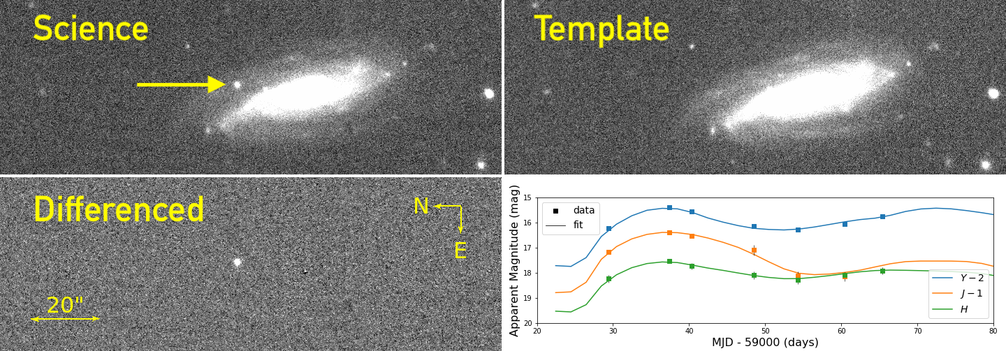
Figure 1: Example images and LC from SN 2020npb. Images span 60”$\times$172” and are taken in the Y-band. Upper Left: Science image from MJD 59029.4 (phase $-12.3$ days relative to optical maximum), the first epoch in the LC. Upper Right: Template image from MJD 59472.2 (phase $+430.5$ days) taken well over a year past peak brightness. Lower Left: Differenced image of the upper two panels with the template image convolved to fit the science image. Lower Right: SNooPy (Burns et al., 2011, 2014) fit to the LC with magnitude offsets for visualization.

Exposure times for all images in all bands were set at 5 seconds. With 2 sets of 5 jitter pointings all microstepping 4 times, each image therefore totaled 200 seconds of exposed time. Across the 3 bands, each target totaled 600 seconds of exposed time. Accounting for time between exposures, filter flushes, slewing, etc., total overhead time for one SN epoch was $\sim$1400 seconds (0.4 hours).

By measuring the magnitudes of the faintest detected stars in each image, we reach a median depth of 20.7, 20.1, and 19.3 mag in Y, J, and H, respectively (with standard deviations of 0.6, 0.8, and 0.6 mag). In the upper-left panel of Fig. 1, we present an example science image from SN 2020npb. The SN itself can be seen offset from the galaxy as indicated by the green arrow a few arcseconds to the upper left of the galaxy.

2.4 Template Images

Template images for the DEHVILS survey were taken in all cases more than a year after our first epoch. Templates were observed and reduced in the exact same way as the corresponding science images except that we doubled the exposure time and required better seeing of $<1.6$ arcseconds. The increased exposure time was used to obtain better depth in our template images than in our science images. The seeing requirement for the template images was modified so that the template image PSFs could be convolved to match the corresponding science image PSFs when performing difference imaging. An example template image is provided in the upper-right panel of Fig. 1 which was taken for SN 2020npb more than a year after peak brightness. When comparing to the corresponding science image to its left, one can see that by eye the SN light is undetectable in the template image.

2.4.1 Archival Templates

Where available, we used images taken as a part of the UKIRT Infrared Deep Sky Survey (UKIDSS; Lawrence et al., 2007) and the UKIRT Hemisphere Survey (UHS; Dye et al., 2018) samples as templates rather than obtaining our own. The UKIDSS survey ran from 2005–2012, and the images we obtained from UKIDSS come primarily from the Large Area Survey, but all surveys are queried using the UKIDSSDR11PLUS data release. Each survey covers approximately 12,700 and 7,000 degrees² for UHS and UKIDSS respectively.

Images from both UKIDSS and UHS have been published online and were taken on the same instrument (WFCAM) and same telescope (UKIRT) as our sample. Images are obtained using astroquery (Ginsburg et al., 2019) and coadded and stitched together using SWarp (Bertin et al., 2002) to construct the templates. Since these surveys did not use microstepping, images from these surveys have a larger pixel scale of 0.4 arcseconds/pixel; therefore, when using the archival templates, we resample our corresponding science images to 0.4 arcseconds/pixel using SWarp.

Archival J-band templates were obtained from UHS. We obtained archival UKIDSS templates for Y and H-bands but our own templates for J-band in the UKIDSS regions. When archival UKIDSS templates for J-band became accessible for us, we utilized those images as well. In total, we use 84 archival template images: 14 in Y, 55 in J, and 15 in H. Since we implement template subtraction for all science images, the remaining 204 template images required come from DEHVILS as described previously.

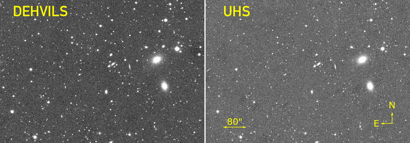
Figure 2: Comparing cutouts from a J-band DEHVILS template to an archival J-band template image for SN 2020uec. Left: Obtained by our program as described in Sections 2.3 and 2.4. Right: Obtained from UHS as described in Section 2.4.1.

In Fig. 2, we compare cutouts from an example DEHVILS template and an archival template from UHS taken at the same location (the SN 2020uec field) and in the same band (J). In many cases, due to the stitching together of multiple survey images, regions of the archival template images that we construct are poor. An effect from this stitching can be seen down the middle of the UHS template. Additionally, the DEHVILS templates have a smaller pixel scale than the archival templates, so we opt for our own template in the few cases where an archival template was also available.

2.5 Optical Data

Optical data for our analysis come from the ATLAS project (Tonry et al., 2018). ATLAS samples the accessible night sky from Hawaii on a near two-day cadence in the optical c and o-bands which span 4200–6500 Å and 5600–8200 Å, respectively. The survey reaches a depth of o $\sim 20$ mag and covers the complete northern sky as well as much of the southern sky down to $\delta\sim-45\degree$. ATLAS images are photometrically calibrated using Pan-STARRS (Chambers et al., 2016). LCs from ATLAS are publicly available, and all DEHVILS SN LCs have a corresponding ATLAS LC (Smith et al., 2020). Optical data from ZTF (Bellm et al., 2019; Förster et al., 2021) are also available for many of the SNe presented here. An analysis on incorporating data from ZTF will be performed in future work from DEHVILS.

2.6 Redshifts

Redshifts come from a variety of sources with host galaxies identified primarily as the nearest neighbor (each SN was inspected individually for assignment). The University of Hawaii 88-inch telescope (UH88) spectra were analyzed with the same methodology used in Section 6 of Williams et al. (2020), the exception being that we avoid the dichroic feature in each SuperNova Integral-Field Spectrograph (SNIFS; Lantz et al., 2004) spectrum by performing independent cross-correlations for the blue channel ($<5070$ Å) and red channel ($>5170$ Å). We then visually compare a template spectrum and the two halves of the SNIFS spectrum and use a weighted average as the observed redshift. The literature sources are from HyperLEDA, which uses multiple published redshift values and a proprietary weighting scheme to estimate the recessional velocity. Additional redshifts are obtained from Subaru spectra using the same method as used on SNIFS spectra, except for the red/blue separation because the Faint Object Camera and Spectrograph (FOCAS; Kashikawa et al., 2002) is a slit spectrograph. 68% of the redshifts come from the literature, 20% from SNIFS, and 12% from Subaru.

Following the cuts listed in Table 1, we present the DEHVILS redshift distribution in comparison to other NIR SN Ia redshift distributions from the literature in Fig. 3. RAISIN SNe are not included in the figure since their redshifts are all $>0.1$. Again, we emphasize that the cuts applied are not definitive statements on which SNe should be used in cosmological analyses (our final sample of SNe on the Hubble diagram is a set of 47 SNe from DEHVILS after cuts, rather than the 67 presented in the right panel of Fig. 3), but the figure is instead intended to provide the reader with a sense of how DEHVILS redshifts compare to those from other surveys in the literature.

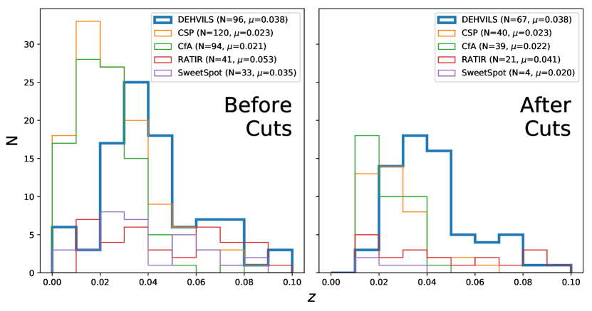
Figure 3: Distribution of redshifts for DEHVILS SNe and SNe from the literature in the first (before cuts; left panel) and final (after cuts; right panel) lines of Table 1.

2.7 Classification

The classifications for DEHVILS SNe come primarily from ZTF. The second-most common group confirming our targets as Type Ia is SIRAH. Other classifying groups given in Table LABEL:tab:SNe include the University of California Santa Cruz (UCSC) Transients Team, Spectroscopic Classification of Astronomical Transients (SCAT; Tucker et al., 2022), the extended-Public ESO Spectroscopic Survey for Transient Objects (ePESSTO+; Smartt et al., 2015), Balcon (2020a, b, 2021), Galbany et al. (2020a, b), DEHVILS (Jha et al., 2020a, c), Soraisam et al. (2020), Pellegrino et al. (2020), accurate determination of H₀ with core-collapse supernovae (adH0cc; Floers et al., 2020), the Global SN Project (Burke et al., 2021), and the Distance Less Than 40 Mpc survey (DLT40; Yang et al., 2019; Wyatt, 2021). The DEHVILS classifications come from spectra obtained using the Robert Stobie Spectrograph (RSS) on the Southern African Large Telescope (SALT).

3 Data Reduction

Initial reductions for our images from UKIRT are done before we receive the data. The microstepping and jittering steps are processed and coadded (averaging counts across jitter steps), and the darks and the sky flats for the evening are applied as corrections so that we receive a single semi-processed image with four extensions, one for each camera (Mike Irwin, private communication).

After the initial reductions, we average counts from both WFCAM’s Camera 3 and Camera 2 (image acquisition detailed in Section 2.3), and we construct mask and noise images given our image characteristics. Given that the saturation point for WFCAM is $\sim$60,000–70,000 counts, we set the masking threshold at 40,000 counts as to avoid regions with possible count-rate nonlinearity. Noise images are computed from the expected poisson noise because read noise for our images is subdominant.

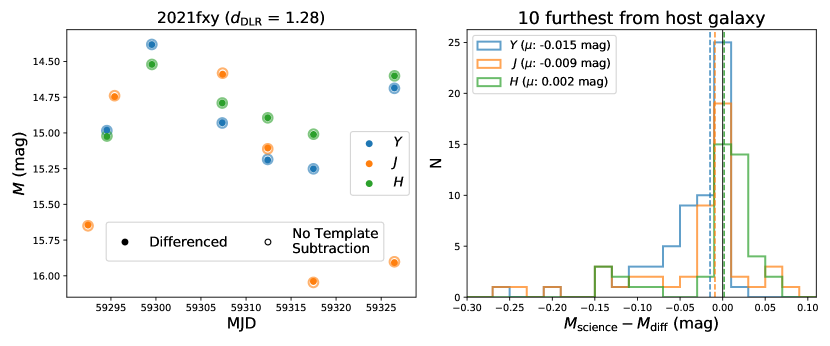
Figure 4: Comparing photometry with and without utilizing a template for galaxy subtraction for SNe relatively far from their host galaxy. Left: Photometry with difference imaging (filled points) and without differencing (unfilled points) for SN 2021fxy which has a large $d_{\textrm{DLR}}$ (angular distance/host galaxy directional light radius). Right: Residual magnitudes for all epochs comparing with and without differencing for the ten SNe found furthest from their host galaxy. Median values are reported in the legend and plotted as dotted lines. Outliers in this panel are due to clear galaxy contamination viewable by eye for SN 2020jdo and SN 2020swy in Y and J.

Further processing for DEHVILS is based on photpipe (Rest et al., 2005, 2014), which is a photometric pipeline that takes SN and template images and outputs calibrated, difference-imaged, forced-photometry LCs. The photpipe reduction pipeline, adapted for the DEHVILS survey here, incorporates the following steps:

1. Photometry: PSF Photometry is performed on sources in the science and template images with the DoPHOT software (Schechter et al., 1993). Stellar detections from this stage are saved and used later in the analysis.

2. Calibration: The 2MASS database is queried for sources within a given WFCAM image footprint. 2MASS JH magnitudes are transformed to YJH magnitudes in the WFCAM natural system following Hodgkin et al. (2009). Existing DoPHOT photometry for point sources in each image is then compared to the transformed 2MASS photometry in order to calculate a zeropoint. Magnitudes are further refined using Hubble Space Telescope (HST) CALSPEC standard stars. Details on calibration are given in Section 4.

3. Difference Imaging: After astrometric alignment of the science and template images, difference imaging is carried out using the image subtraction software High Order Transform of PSF ANd Template Subtraction (HOTPANTS; Becker, 2015) which uses the Alard & Lupton algorithm (Alard & Lupton, 1998; Alard, 2000). This procedure convolves the template image with three best-fit Gaussian kernels to match the PSF of the science image, scales the template image such that both images have the same zeropoint, and subtracts the template image from the science image.

   Alternatively, one could convolve the science images to match the template images; however, our seeing requirement for template images was more restrictive than for the science images and therefore, the average seeing for template images was better than that of the science images. As a result, in all cases we convolved the template image to match the PSF of the science image prior to image subtraction.

   We present an example differenced image in the lower-left panel of Fig. 1.

4. Photometry on the Differenced Image and Final Checks: DoPHOT photometry is performed on the differenced images to determine a weighted-average centroid for each SN. Final forced-photometry LCs including non-detections are produced, again using DoPHOT, for each SN using this centroid.

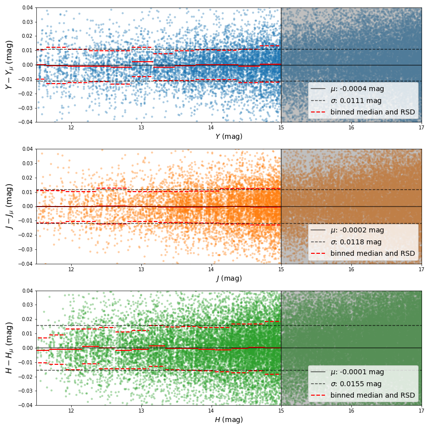
Figure 5: Testing the repeatability of obtaining a given magnitude for a star by taking the distribution of observed magnitudes for that star and comparing it to the mean. Individual magnitudes are compared to the mean magnitude and plotted as a function of magnitude. Binned statistics are plotted in red, and the overall median and RSD of the residuals for all stars brighter than 15 mag are reported in the legend.

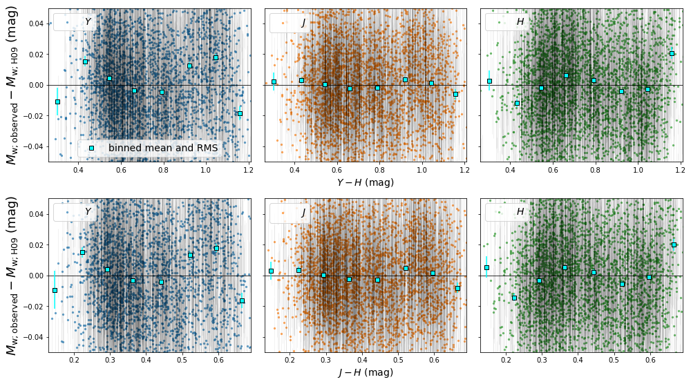
Figure 6: Residual (observed minus transformed from 2MASS) YJH WFCAM magnitudes for all stars detected in our sample with respect to color (both Y$-$H and J$-$H using transformed magnitudes). Binned means with RMS are also provided.

3.1 Validating Image Subtraction

For the ten SNe furthest from their host galaxy, which were designated using a parameter that uses the angular distance normalized by the host galaxy’s directional light radius (DLR; variable dependent on the galaxy’s shape and direction to the SN) called $d_{\textrm{DLR}}$ (Gupta et al., 2016; Sako et al., 2018), photometry could be done on the SN alone and a LC could be constructed without image subtraction. The $d_{\textrm{DLR}}$ values were obtained using the Galaxies HOsting Supernovae and other Transients (GHOST; Gagliano et al., 2021) program which identifies likely host galaxies for each SN. These ten SNe all have $d_{\textrm{DLR}}$ values $>0.98$ meaning their angular separations are all close to if not larger than the host galaxy’s DLR, and they provide us with a consistency check for our difference imaging analysis. The left panel of Fig. 4 depicts how similar LCs (with and without subtraction) are for an example SN designated as far from the galaxy. For SN 2021fxy, all observations without subtraction are consistent with the values obtained with template subtraction. In the right panel of Fig. 4, we present the distribution of residual magnitudes with and without template subtraction observing median residuals of $-0.009$ mag and $0.002$ mag for J and H, respectively, each near zero. The robust median absolute standard deviation (RSD, Hoaglin et al. (2000); defined by applying a factor of 1.48 to the median of the absolute values of the deviations of the residuals from the median residual) of these residual magnitudes are 0.022 mag and 0.023 mag. We see the largest deviation from zero in Y-band at $-0.015$ mag (0.026 mag RSD) indicating photometry on images without subtraction may result in slightly brighter SN magnitudes — potentially due to galaxy contamination.

3.2 Repeatability of Stellar Magnitudes

We check our photometric precision by calculating the repeatability floor of the stars in our sample in Fig. 5. We compile stellar detections from all images for 30 of our SNe, calculating the derived magnitude for all stars across all images for each SN. The mean magnitude of each star’s distribution of magnitudes is calculated and used to compare distributions of magnitudes across the sample. Only stars detected at 15th magnitude or brighter are used (the unshaded region of the figure). We obtain RSD values of 0.0111, 0.0118, and 0.0155 mag for Y, J, and H respectively, and as a result, we use 0.0150 mag as our repeatability floor. Thus, we include this as an additional error to the calculated SN magnitudes and magnitude errors obtained from the reduction pipeline described in Section 3.

4 Calibration

The general calibration strategy is as follows:

1. To determine calibration zeropoints for each image, we use photometry from the Two Micron All Sky Survey (2MASS; Skrutskie et al., 2006) as it has full sky coverage in JHK across our complete survey footprint. This photometry must be transformed to that expected from WFCAM.

2. To define an absolute calibration, we compute single offsets for each filter by comparing photometry we obtain of HST standard stars in the CALSPEC database (Bohlin et al., 2014, 2020) to predicted synthetic magnitudes from WFCAM.

4.1 Calibration Zeropoints for each Image

To transform the 2MASS photometry to WFCAM magnitudes, we follow Hodgkin et al. (2009) (hereafter H09). The specific transformations for the filters we use are:

$$Y_{\textrm{w}}=J_{2}+0.500(J_{2}-H_{2})+0.080,$$ (1)

$$J_{\textrm{w}}=J_{2}+0.065(J_{2}-H_{2}),$$ (2)

$$H_{\textrm{w}}=H_{2}+0.070(J_{2}-H_{2})-0.030.$$ (3)

YJH with subscripts w are filter values for WFCAM and are transformed from JH 2MASS bands (with subscript 2). As can be inferred from Eq. 1, 2MASS did not have a Y-band filter; 2MASS used JHK bands.

When we compare our observed stellar magnitudes ($M_{\textrm{w; observed}}$) to the derived WFCAM magnitudes from the 2MASS catalog ($M_{\textrm{w; H09}}$; obtained using Eqs. 1, 2, and 3), we observe the differences in magnitude of the two as a function of color. We present these residuals as a function of Y$-$H and J$-$H colors in Fig. 6. We find that across all comparisons when splitting the distributions into bins, the calibrations are reliable down to $2\%$ — consistent with the findings of H09. However, we do observe bright stars as $\sim$0.02 mag too bright and magnitude dependent trends in YJH of $\sim$8 mmag/mag, $\sim$4 mmag/mag, and $\sim$2 mmag/mag, respectively, but we attribute this to nonlinearity of either the 2MASS or WFCAM detector.

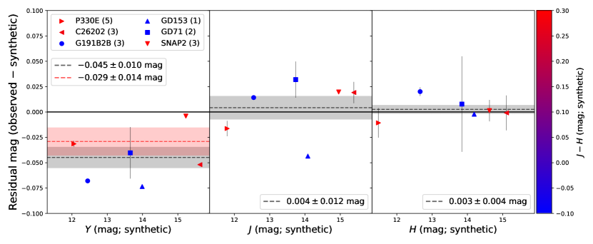
Figure 7: Comparing observed magnitudes to synthetically obtained magnitudes by integrating over the WFCAM bandpasses for six CALSPEC standard stars on the Vega magnitude system. Observed magnitudes are calculated using the obtained flux and the transformation equations from H09 in the zeropoint calculation. For each star, the number of observations from which the mean and standard error on the mean are calculated is reported in the legend. A best-fit offset and relative error is also provided in each panel with an additional fit to the three reddest stars in the Y-band panel. J$-$H colors are depicted as well.

4.2 Absolute Calibration Using HST CALSPEC Stars

We take observations of HST CALSPEC standard stars in order to further validate and/or improve upon the calibration of our sample. HST spectra from these CALSPEC standard stars are described in Bohlin et al. (2014, 2020) and obtained online. Synthetic magnitudes are calculated using those spectra and integrating over the WFCAM YJH bandpasses. These synthetic magnitudes are then compared to the observed magnitudes for each of these standard stars in Fig. 7 on the Vega magnitude system. Most standard stars were observed multiple times, so we provide the mean observed magnitude and standard error on the mean. Each panel is fit for an offset from zero in gray. J$-$H color information is provided on a color scale from blue to red. We observe that with the current calibration system J and H seem to be calibrated well (median offsets of $0.004\pm 0.012$ mag and $0.003\pm 0.004$ mag, respectively), but Y demonstrates a significant offset from zero at $-0.045\pm 0.010$ mag.

We present an additional fit in red to the three reddest CALSPEC stars in the Y-band panel of Fig. 7. As can be seen from Fig. 6, these stars, with J$-$H colors ranging from 0.278–0.331 mag, are the CALSPEC stars most similar (in terms of J$-$H color) to the stars used to compute zeropoints for DEHVILS. These three redder stars demonstrate a smaller offset from zero than the full sample of CALSPEC stars in Y band, but the offset is still significant at $-0.029\pm 0.014$ mag. Given this finding, we add 0.029 mag to all of our SN LC Y-band magnitudes and consider the difference between this calculated offset and the offset from the complete CALSPEC sample as a systematic that should be incorporated in cosmological analyses using DEHVILS data. Additional observations of CALSPEC standard stars will help refine this correction.

5 Light Curve Model Descriptions and Fits

We use the SNANA software package (Kessler et al., 2009, 2019) to fit our LCs using both SALT3 (Pierel et al., 2022) and SNooPy (Burns et al., 2011, 2014). SNANA is a package that can estimate LC parameters, simulate SN samples, measure distances, and fit for cosmological parameters. Additional fits are done using BayeSN (Mandel et al., 2022; Ward et al., 2022). For NIR-only fits, the time of maximum is constrained using the optical ATLAS data.

5.1 SALT3

We use the SALT3 model (Kenworthy et al., 2021) for LC fits, but specifically we test the extension to the NIR described in Pierel et al. (2022). The SALT3 model extension is trained on $\sim$1000 LCs with data in the optical bands and 166 LCs with data in the NIR (including data from this sample). SALT3 is also trained with both optical and NIR spectra to build in K-corrections. SALT3 fits for a LC stretch, $x_{1}$, a LC color, $c$, and an amplitude, $x_{0}$ and uses an equation with flux, $f$, wavelength, $\lambda$, phase, $p$, $M_{0}$ and $M_{1}$ as phase-factors on $x_{0}$ and $x_{1}$ describing the spectral energy distribution (SED), and CL as a color law inputted into the model. This extension to the SALT3 model (Pierel et al., 2022), used for all of our NIR-only, NIR+optical, and optical-only SALT3 fits, expands on the SALT3 model (Kenworthy et al., 2021) by extending the $M_{0}$ and $M_{1}$ wavelength ranges and defining the color law out to 20,000 Å each.

When fitted using the SALT3 model, each LC has a best fit $x_{0}$, $x_{1}$, and $c$ value which is then incorporated in the Tripp equation (Tripp, 1998) in order to obtain a distance modulus, $\mu$,

$$\mu=m_{B}+{\alpha}x_{1}-{\beta}c-\mathcal{M}$$ (4)

where $m_{B}$ is the apparent SN peak magnitude in the $B$ band and directly related to $x_{0}$ ($m_{B}=-2.5\log(x_{0})+const.$), $\alpha$ and $\beta$ are the regression coefficients that relate $x_{1}$ and $c$, respectively, to a luminosity correction, and $\mathcal{M}$ is the globally fit absolute SN peak magnitude (for a SN with $c,x_{1}=0,0$). When using SALT3 on NIR data, because of the extended framework presented by Pierel et al. (2022), NIR SN LCs are fit in much the same way as in the optical.

Table 3: SALT3 Fit Parameters and Hubble Residual Scatter

Filters	PV Corr.	$x_{1}$	$c$	$\alpha$	$\beta$	N fit	RSD	STD
							(mag)	(mag)
YJH	No	fixed	fixed	0.000	0.000	47	0.139 $\pm$ 0.026	0.172 $\pm$ 0.027
coYJH	No	floated	floated	0.075 $\pm$ 0.034	2.903 $\pm$ 0.223	47	0.132 $\pm$ 0.025	0.175 $\pm$ 0.034
co	No	floated	floated	0.145 $\pm$ 0.043	2.359 $\pm$ 0.249	47	0.177 $\pm$ 0.029	0.221 $\pm$ 0.043
YJH	Yes	fixed	fixed	0.000	0.000	47	0.102 $\pm$ 0.018	0.128 $\pm$ 0.015
coYJH	Yes	floated	floated	0.073 $\pm$ 0.025	2.753 $\pm$ 0.161	47	0.119 $\pm$ 0.019	0.128 $\pm$ 0.016
co	Yes	floated	floated	0.140 $\pm$ 0.034	2.349 $\pm$ 0.190	47	0.141 $\pm$ 0.033	0.169 $\pm$ 0.023

5.2 SNooPy

SNooPy (Burns et al., 2011, 2014) is a model that has been used widely for NIR LC fitting. SNooPy has been trained on well-calibrated CSP LCs with templates across uBVgriYJH bands. Fitted parameters for SNooPy include a time of maximum, $T_{\textrm{max}}$, a color-stretch parameter that is a measure of how quickly the SN reaches maximum $B-V$ color, $s_{BV}$, and parameters related to dust; the Milky Way’s (MW) color excess $E(B-V)_{\textrm{MW}}$, the host galaxy’s color excess $E(B-V)_{\textrm{host}}$, and the ratio of total to selective absorption $R_{V}$. We use SNooPy’s EBV_model2 fixing $s_{BV}=1$, $A_{V}=0$, and $E(B-V)_{\textrm{host}}=0$ to fit the NIR-only LCs in SNANA following Jones et al. (2022). We also fix the time of maximum to the value determined from the optical data; therefore, the only free parameter in the SNooPy fits is the overall SN amplitude.

5.3 BayeSN

Another LC fitter trained on NIR data is BayeSN (Thorp et al., 2021; Mandel et al., 2022; Ward et al., 2022). BayeSN employs a hierarchical Bayesian approach to modeling SNe Ia, generalizing the previous LC model of Mandel et al. (2011). BayeSN is a probabilistic time-dependent SED model which leverages both optical and NIR data to infer host galaxy dust parameters and intrinsic spectral components. Specifically, BayeSN fits the LCs for a distance modulus, $\mu$, the coefficient of the first functional principal component, $\theta$ (correlated strongly with stretch but also includes intrinsic color), and extinction, $A_{V}$. For the BayeSN fits, we use the M20 version described in Mandel et al. (2022). Because we are fitting only NIR data, where the sensitivity to dust is minimal, we fix $A_{V}=0$ and $\theta=-1$ (corresponding to $s_{BV}\approx 1$).

6 Hubble Diagram

The distance modulus values for the DEHVILS SNe that are fit using SALT3 and SNooPy are calculated using SNANA. LC quality cuts for the DEHVILS data are defined as follows: SALT3 $|x_{1}|<3$, uncertainty on SALT3 $x_{1}<1$, uncertainty on the peak MJD $<2$ days, $E(B-V)_{\textrm{MW}}<0.2$, and Type Ia LC fit probability (defined by SNANA) $>0.01$. Typical LC cuts also include a cut on SALT3 $|c|<0.3$ and uncertainty on SALT3 $c<0.05$, but in the case of NIR-only LC fits, $c$ is often unconstrainable because NIR magnitude is largely degenerate with the $c$ parameter. Thus, we do not include a color constraint in these cases. In total, 47 out of 83 SNe Ia satisfy all cuts. The LC fit probability cut causes the greatest loss, cutting 40 of the the 46 removed; by visual inspection, we believe the model errors are likely underestimated leading to low fit probabilities, but we leave redevelopment of this model to a future work.

Hubble diagrams are constructed using (i) the $\mu$ values derived from the fitted LC parameters and a modified version of Eq. 4, depending on which corrections are applied (i.e., stretch, color, mass step; could be simply $\mu=m_{B}-\mathcal{M}$) and (ii) the spectroscopic host redshifts obtained, which are corrected into the Cosmic Microwave Background (CMB) frame. Where indicated, peculiar velocity (PV) corrections are also applied to the redshifts according to Peterson et al. (2022) utilizing the recommended group and coherent-flow corrections.

For measurements of scatter on the Hubble diagram, we calculate the RSD for each of our fitting procedures as the median of the absolute values of the deviations of the Hubble residuals ($\Delta_{\mu}=\mu-\mu(z)$) from the median residual multiplied by 1.48,

$$\textrm{RSD}=1.48\times\textrm{median}\big{(}|\Delta_{\mu}-\textrm{median}(\Delta_{\mu})|\big{)},$$ (5)

where $\mu(z)$ is the predicted distance with a given redshift and a fiducial cosmology. The sample standard deviation (STD) of the $\mu$ residuals is also provided. We provide a measurement of the uncertainty in these scatter values using bootstrapping. We recalculate each scatter value (both RSDs and STDs) choosing the 47 $\mu$ residuals at random, with replacement, 5000 times and take the STD of that sample as a measure of uncertainty for the scatter values given in Table 3.

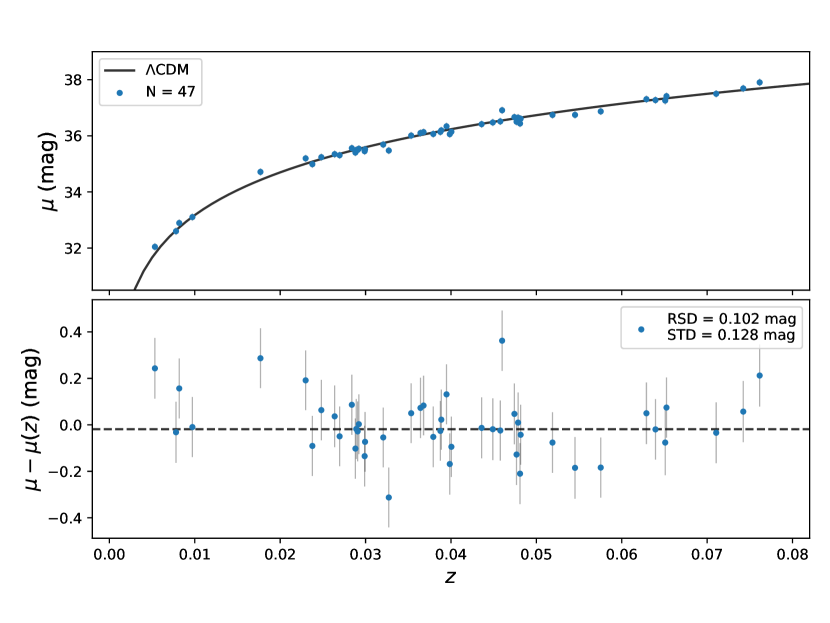
Figure 8: Hubble diagram (top) and Hubble residuals (bottom) for a NIR-only SALT3 fit with the LC parameters $x_{1}$ and $c$ fixed to zero and PV corrections applied. The dotted line indicates the median Hubble residual of the sample.

Studies have claimed that omitting stretch/color corrections in the NIR yields distance measurements with minimal scatter, indicating SNe Ia in the NIR are more nearly standard candles (Dhawan et al., 2018; Avelino et al., 2019; Pierel et al., 2022; Galbany et al., 2022). We test both the omission and inclusion of stretch/color corrections as well as the omission and inclusion of optical data on fits using SALT3. Results from these tests are presented in Table 3. We observe that when comparing NIR-only (YJH) SALT3 fits to NIR+optical (coYJH) SALT3 fits, scatter is smaller for the NIR-only fits in all cases except for the RSD value without PV corrections. The inclusion of PV corrections results in improved RSD and STD values for all cases. When we float $x_{1}$ while keeping $c$ fixed to zero for NIR-only fits, the scatter increases but the errors on $\alpha$ also increase significantly. When treating the SNe as perfect standard candles for NIR-only fits (fixing both $x_{1}=0$ and $c=0$), we observe RSD and STD values of 0.139 mag and 0.172 mag without using PV corrections. Treating the DEHVILS SNe as standard candles, using only NIR data, and including PV corrections results in the most favorable scatter values (RSD of 0.102 mag and STD of 0.128 mag) in Table 3.

Table 4: LC Model Hubble Residual Scatter Comparison

Model	Filters	N fit	PV Corr.	RSD	STD
				(mag)	(mag)
SALT3a	YJH	47	No	0.139 $\pm$ 0.026	0.172 $\pm$ 0.027
SNooPy	YJH	47	No	0.162 $\pm$ 0.037	0.177 $\pm$ 0.031
BayeSN	YJH	47	No	0.115 $\pm$ 0.033	0.180 $\pm$ 0.032
SALT3a	YJH	47	Yes	0.102 $\pm$ 0.018	0.128 $\pm$ 0.016
SNooPy	YJH	47	Yes	0.093 $\pm$ 0.026	0.135 $\pm$ 0.016
BayeSN	YJH	47	Yes	0.094 $\pm$ 0.025	0.131 $\pm$ 0.015

• fixed $x_{1}=0$ and fixed $c=0$ from Table 3.

We present an example Hubble diagram with Hubble residuals with respect to a fiducial cosmology in Fig. 8 which has its results listed in Table 3. The Hubble diagram provided is from the SALT3 fit, fixing both $x_{1}=0$ and $c=0$ and fitting NIR-only (YJH) with PV corrections applied. When comparing these NIR-only Hubble residuals to the optical-only fitted parameters $x_{1}$ and $c$, we find no significant correlations ($<2\sigma$ detections of a correlation in each case). The distance uncertainties obtained for this sample are likely underestimated with the SALT3 fitting process in the NIR (median of 0.030 mag). Therefore, the derived intrinsic scatter, $\sigma_{\textrm{int}}$, to make the reduced $\chi^{2}$ set to unity for this sample is 0.126 mag, which dominates the errors on $\mu$ in Fig. 8.

Hubble residual scatter values from all LC fitters are given in Table 4. Uncertainties on those scatter values are provided and calculated using the same bootstrapping method as described above for Table 3. To ensure a valid comparison between LC models, we use the same SNe in calculating all scatter values, and LC model fits are NIR-only. Additionally, we fix similar parameters across each model. For SALT3, we fix both $x_{1}=0$ and $c=0$; for SNooPy, we fix $A_{V}=0$ and $s_{BV}=1$; and for BayeSN we fix $A_{V}=0$ and $\theta=-1$. All LC models are competitive. SALT3, SNooPy, and BayeSN exhibit similar results in terms of RSD and STD values. In terms of RSD, scatter on the Hubble diagram before PV corrections are applied ranges 0.115–0.162 mag and after PV corrections are applied ranges 0.093–0.102 mag. In terms of STD, all models exhibit similar values of $\sim$0.175 mag without PV corrections and $\sim$0.130 mag with PV corrections.

Using the redshift-based distance $\mu(z)$ based on a fiducial cosmology, we present composite YJH LCs in Fig. 9 for the 47 SNe passing cuts. Individual SN LCs are aligned with respect to phase relative to optical maximum and brightness by subtracting $\mu(z)$ values from each SN LC’s apparent magnitudes. A Gaussian Process regression line is provided in Fig. 9 along with its STD presented in gray for each filter. STD values in the DEHVILS composite LCs are 0.189, 0.248, and 0.194 mag at optical maximum for Y, J, and H, respectively. These results demonstrate how viable treating SNe Ia as standard candles is in the NIR.

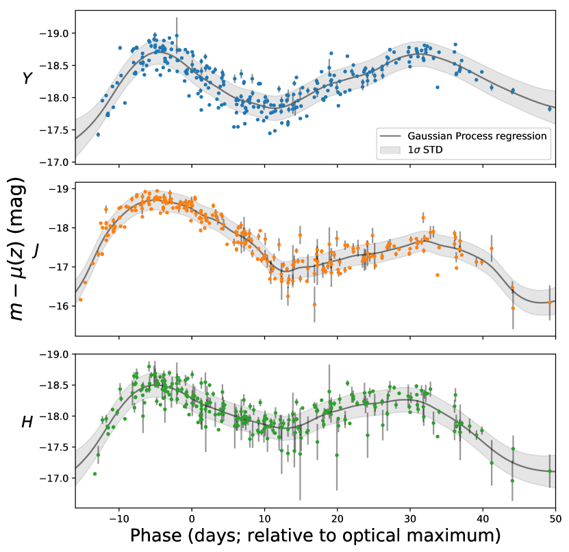
Figure 9: Composite YJH LCs for the 47 SNe presented in Fig. 8. Individual SN LCs are aligned horizontally by phase and vertically by taking the apparent magnitudes and subtracting the redshift-based distance $\mu(z)$ based on a fiducial cosmology. The data are fit using a Gaussian Process regression, and a 1$\sigma$ confidence interval is indicated in gray.

7 Discussion

This initial DEHVILS data release is a sizable contribution to the current publicly available NIR SN Ia LC sample. In the literature, there are still $\lesssim$ 200 NIR SN Ia LCs with a coverage and cadence similar to DEHVILS. We contribute an additional 83 such LCs to the field. For the 47 SNe which pass strict SALT3 cuts, we find the best scatter (an RSD value of 0.093 mag) on the Hubble diagram comes from using NIR-only filters, fixing SNooPy $A_{V}$ and SNooPy $s_{BV}$, and utilizing PV corrections in Table 4. We note that, for SALT3, the inclusion of optical ATLAS data in the fits results in worse scatter in most cases; in part, this may be due to the fact that the SALT3 model uncertainties do not include off-diagonal covariance to aid in the weighting of data at different wavelengths at this time. Comparing to the literature, Stanishev et al. (2018) compile a sample of $\sim$120 single-band (J and H) LCs (including data from CSP and CfA) for root-mean-square (RMS) values of $\sim$0.14–0.15 mag. Johansson et al. (2021) report single-band (J and H) RMS values of $\sim$0.2 mag when combining their data from RATIR with SNe from the literature (e.g., from CSP and CfA) for a total of $\sim$160 SNe and fitting with SNooPy. Pierel et al. (2022) find a NIR-only RMS value of 0.126 mag using SALT3 and a sample of 24 SNe (including a few from this data release).

We aimed for NIR LCs with good sample coverage and achieved a sample average of $\sim$6 epochs in three different bands. Work has been done previously to ascertain how many epochs and what quality of observations are necessary for good cosmological results with both NIR and optical data (Stanishev et al., 2018; Müller-Bravo et al., 2022). The findings from these works suggest that NIR epochs need not be plentiful ($\sim$1–2 epochs in a single band) nor outstanding in quality (signal-to-noise $\gtrsim$ 8 in H) in order to precisely measure cosmological parameters as long as the epochs are near NIR-peak. We encourage future works to utilize our data to further test this hypothesis.

In future work, we intend to test a wider range of fitting parameters compared to those presented in both Table 3 and Table 4. For example, we will test single-filter fits and combinations of filters. We plan to examine the effects from using or not using various LC model fitting parameters and from the inclusion of optical data for SNooPy and BayeSN fits. Given that our quality cuts are focused on the SALT3 parameters and LC fit metric, we recognize that the scatter results on the selected subsample are likely to favor the SALT3 model, and thus may underestimate the true variation in the NIR LCs. We also intend to present results from different LC quality-cut criteria (such as cuts focused on results from BayeSN fits) and results from combining our data with LCs in the literature. An analysis on a DEHVILS NIR mass step value will also be included in future work.

We also encourage future work to be done on testing the 2MASS to WFCAM filter transformation equations, specifically in the Y-band. Given our HST CALSPEC standard star analysis, we add an additional 0.029 mag to all Y-band SN magnitudes as a part of our absolute calibration. This systematic could be further tested, for example, with HST observations of the stars in our SN fields. Analyzing a potential zeropoint systematic due to variation across the field is another goal for future work from DEHVILS.

8 Conclusions

In this data release, we present 83 SN Ia LCs. We describe both our data reduction pipeline and calibration and confirm that neither introduces significant errors into our analysis. We validate our HOTPANTS difference imaging process by comparing photometry done on both template-subtracted and unsubtracted images. We confirm that our calibration is reliable to 2% by comparing obtained stellar magnitudes to transformed 2MASS catalog stellar magnitudes, and we further refine our calibration by comparing obtained magnitudes to magnitudes synthetically obtained from spectra for HST CALSPEC stars. We conclude that the J and H bands are calibrated well, but we find a magnitude offset in Y band of 0.029 $\pm$ 0.014 mag indicating our initial derived Y-band magnitudes were slightly too bright. We correct for this offset and report our results.

Of the 83 SN Ia LCs, 47 make it through strict SALT3 quality cuts. We report scatter on the Hubble diagram for these 47 SNe to be $\lesssim$ 0.1 mag using NIR-only fits for the DEHVILS sample which is better than the scatter reported for optical-only Hubble diagrams at $\sim$0.15–0.17 mag (Betoule et al., 2014; Brout et al., 2022). This supports the finding that SNe Ia are excellent standard candles in the NIR. We find that all the LC models tested here exhibit similar amounts of scatter on the Hubble diagram.

SN Ia cosmology with Roman will require an anchor sample, preferably in the NIR, with comparable precision in calibration and limited systematics. Continued work and further observations from DEHVILS must be done to achieve this. The DEHVILS data outlined here have been released to the public at https://github.com/erikpeterson23/DEHVILSDR1. Additional data from the DEHVILS survey targeting Cepheids have been published (Konchady et al., 2022).

Software

SNANA (Kessler et al., 2009), astropy (Astropy Collaboration et al., 2013; Price-Whelan et al., 2018), matplotlib (Hunter, 2007), numpy (Van Der Walt et al., 2011), PIPPIN (Hinton & Brout, 2020), astroquery (Ginsburg et al., 2019), SWarp (Bertin, 2010).

Data Availability

The data are available on GitHub at https://github.com/erikpeterson23/DEHVILSDR1.

Table 5: Optical-only SALT3 fit results

SN	Optical Peak MJD	SALT3 $x_{1}$	SALT3 $c$
	(days)
2020fxa	58958.6 $\pm$ 0.3	0.89 $\pm$ 0.22	$-$0.07 $\pm$ 0.03
2020jdo	58984.1 $\pm$ 0.3	$-$1.84 $\pm$ 0.37	0.18 $\pm$ 0.08
2020jfc	58985.2 $\pm$ 0.1	$-$2.90 $\pm$ 0.19	0.34 $\pm$ 0.05
2020jgl	58993.0 $\pm$ 0.3	$-$0.67 $\pm$ 0.40	$-$0.00 $\pm$ 0.04
2020jht	58990.8 $\pm$ 0.2	1.17 $\pm$ 0.27	0.46 $\pm$ 0.03
2020jio	58993.6 $\pm$ 0.3	5.00 $\pm$ 0.63	0.45 $\pm$ 0.05
2020jjf	58988.2 $\pm$ 0.3	0.16 $\pm$ 0.30	0.04 $\pm$ 0.04
2020jjh	58993.4 $\pm$ 0.2	0.35 $\pm$ 0.18	0.02 $\pm$ 0.03
2020jsa	58992.9 $\pm$ 0.2	$-$1.89 $\pm$ 0.19	0.28 $\pm$ 0.04
2020jwl	58992.4 $\pm$ 0.3	$-$0.25 $\pm$ 0.27	0.00 $\pm$ 0.04
2020kav	58989.1 $\pm$ 0.6	$-$1.69 $\pm$ 0.62	$-$0.08 $\pm$ 0.06
2020kaz	58992.5 $\pm$ 0.2	0.56 $\pm$ 0.28	$-$0.19 $\pm$ 0.04
2020kbw	58997.1 $\pm$ 0.3	0.02 $\pm$ 0.36	0.02 $\pm$ 0.06
2020kcr	58998.2 $\pm$ 0.3	5.00 $\pm$ 0.04	0.35 $\pm$ 0.06
2020khm	58993.0 $\pm$ 0.4	$-$2.20 $\pm$ 0.61	$-$0.06 $\pm$ 0.08
2020kkc	58998.5 $\pm$ 0.2	$-$0.06 $\pm$ 0.28	0.12 $\pm$ 0.05
2020kku	58995.3 $\pm$ 0.3	$-$2.43 $\pm$ 0.37	0.34 $\pm$ 0.07
2020kpx	59004.7 $\pm$ 0.1	$-$1.68 $\pm$ 0.11	$-$0.10 $\pm$ 0.04
2020kqv	58997.7 $\pm$ 0.4	$-$0.25 $\pm$ 0.45	$-$0.14 $\pm$ 0.05
2020kru	58997.2 $\pm$ 0.2	$-$1.19 $\pm$ 0.23	0.53 $\pm$ 0.06
2020krw	58999.1 $\pm$ 0.2	$-$1.25 $\pm$ 0.36	0.15 $\pm$ 0.08
2020kyx	59008.8 $\pm$ 0.1	$-$0.53 $\pm$ 0.13	0.08 $\pm$ 0.04
2020kzn	59000.9 $\pm$ 0.3	1.20 $\pm$ 0.34	0.61 $\pm$ 0.07
2020lfe	59009.5 $\pm$ 0.2	0.40 $\pm$ 0.21	$-$0.00 $\pm$ 0.04
2020lil	59011.7 $\pm$ 0.2	$-$1.68 $\pm$ 0.13	0.03 $\pm$ 0.05
2020lsc	59018.2 $\pm$ 0.2	$-$0.26 $\pm$ 0.12	0.03 $\pm$ 0.03
2020lwj	59015.4 $\pm$ 0.2	$-$1.39 $\pm$ 0.21	$-$0.12 $\pm$ 0.05
2020may	59025.1 $\pm$ 0.2	1.66 $\pm$ 0.50	$-$0.13 $\pm$ 0.06
2020mbf	59020.2 $\pm$ 0.2	$-$0.63 $\pm$ 0.18	0.08 $\pm$ 0.04
2020mby	59022.9 $\pm$ 0.2	$-$1.43 $\pm$ 0.12	$-$0.10 $\pm$ 0.05
2020mdd	59016.9 $\pm$ 0.0	$-$1.82 $\pm$ 0.00	$-$0.22 $\pm$ 0.03
2020mnv	59028.3 $\pm$ 0.1	$-$0.53 $\pm$ 0.13	0.00 $\pm$ 0.03
2020mvp	59028.0 $\pm$ 0.2	$-$0.45 $\pm$ 0.22	0.51 $\pm$ 0.05
2020naj	59036.3 $\pm$ 0.2	4.32 $\pm$ 0.33	0.08 $\pm$ 0.03
2020nbo	59028.8 $\pm$ 0.2	$-$2.33 $\pm$ 0.23	0.07 $\pm$ 0.06
2020ndv	59034.3 $\pm$ 0.2	0.52 $\pm$ 0.16	$-$0.08 $\pm$ 0.03
2020ned	59034.6 $\pm$ 0.2	5.00 $\pm$ 0.02	0.68 $\pm$ 0.04
2020nef	59029.7 $\pm$ 0.2	$-$1.38 $\pm$ 0.28	$-$0.16 $\pm$ 0.06
2020npb	59041.7 $\pm$ 0.2	0.76 $\pm$ 0.16	0.02 $\pm$ 0.03
2020nst	59031.6 $\pm$ 0.3	1.21 $\pm$ 0.36	0.47 $\pm$ 0.06
2020nta	59036.1 $\pm$ 0.3	$-$4.32 $\pm$ 0.35	0.56 $\pm$ 0.13
2020ocv	59048.4 $\pm$ 0.3	0.49 $\pm$ 0.34	0.15 $\pm$ 0.05
2020oil	59054.1 $\pm$ 0.2	$-$0.06 $\pm$ 0.17	$-$0.18 $\pm$ 0.04
2020oms	59050.3 $\pm$ 0.3	0.73 $\pm$ 0.25	0.00 $\pm$ 0.04
2020pst	59064.6 $\pm$ 0.2	$-$0.58 $\pm$ 0.20	$-$0.10 $\pm$ 0.04
(continued on next page)
2020qic	59071.1 $\pm$ 0.2	0.31 $\pm$ 0.18	$-$0.13 $\pm$ 0.03
2020qne	59075.1 $\pm$ 0.2	5.00 $\pm$ 0.03	0.50 $\pm$ 0.05
2020rgz	59089.4 $\pm$ 0.1	0.18 $\pm$ 0.13	0.25 $\pm$ 0.03
2020rlj	59088.7 $\pm$ 0.3	$-$2.35 $\pm$ 0.23	0.18 $\pm$ 0.06
2020sjo	59107.6 $\pm$ 0.2	$-$0.57 $\pm$ 0.13	$-$0.03 $\pm$ 0.02
2020sme	59112.9 $\pm$ 0.2	1.85 $\pm$ 0.21	0.08 $\pm$ 0.03
2020svo	59113.5 $\pm$ 0.1	0.45 $\pm$ 0.18	$-$0.06 $\pm$ 0.03
2020swy	59116.1 $\pm$ 0.2	1.08 $\pm$ 0.18	0.16 $\pm$ 0.03
2020szr	59118.0 $\pm$ 0.1	0.39 $\pm$ 0.14	0.07 $\pm$ 0.03
2020tdy	59118.8 $\pm$ 0.3	$-$0.84 $\pm$ 0.36	$-$0.05 $\pm$ 0.07
2020tfc	59114.4 $\pm$ 0.2	$-$2.41 $\pm$ 0.20	$-$0.02 $\pm$ 0.04
2020tkp	59123.9 $\pm$ 0.1	1.02 $\pm$ 0.18	0.27 $\pm$ 0.03
2020tpf	59123.6 $\pm$ 0.2	1.29 $\pm$ 0.23	$-$0.13 $\pm$ 0.03
2020tug	59127.2 $\pm$ 0.2	0.19 $\pm$ 0.27	$-$0.17 $\pm$ 0.04
2020uea	59126.7 $\pm$ 0.1	$-$3.97 $\pm$ 0.20	0.82 $\pm$ 0.09
2020uec	59131.5 $\pm$ 0.2	0.61 $\pm$ 0.16	$-$0.08 $\pm$ 0.03
2020uek	59125.1 $\pm$ 0.1	$-$1.54 $\pm$ 0.16	0.08 $\pm$ 0.04
2020uen	59125.7 $\pm$ 0.0	$-$0.62 $\pm$ 0.16	0.28 $\pm$ 0.04
2020unl	59135.0 $\pm$ 0.2	$-$2.00 $\pm$ 0.17	0.18 $\pm$ 0.03
2020vnr	59142.9 $\pm$ 0.4	1.28 $\pm$ 0.55	$-$0.06 $\pm$ 0.06
2020vwv	59148.4 $\pm$ 0.2	0.73 $\pm$ 0.22	$-$0.05 $\pm$ 0.04
2020wcj	59148.8 $\pm$ 0.2	$-$1.30 $\pm$ 0.15	$-$0.09 $\pm$ 0.03
2020wgr	59148.3 $\pm$ 0.2	0.17 $\pm$ 0.19	0.08 $\pm$ 0.04
2020wtq	59148.8 $\pm$ 0.1	$-$0.76 $\pm$ 0.17	$-$0.04 $\pm$ 0.04
2020yjf	59164.6 $\pm$ 0.3	0.59 $\pm$ 0.23	$-$0.29 $\pm$ 0.05
2020ysl	59162.5 $\pm$ 0.3	$-$1.39 $\pm$ 0.20	$-$0.00 $\pm$ 0.06
2020aczg	59217.4 $\pm$ 0.2	$-$0.04 $\pm$ 0.17	$-$0.13 $\pm$ 0.03
2021ash	59245.7 $\pm$ 0.3	$-$0.35 $\pm$ 0.21	$-$0.19 $\pm$ 0.04
2021aut	59245.0 $\pm$ 0.3	0.03 $\pm$ 0.27	$-$0.11 $\pm$ 0.04
2021bbz	59251.9 $\pm$ 0.4	$-$0.17 $\pm$ 0.17	$-$0.01 $\pm$ 0.03
2021biz	59258.4 $\pm$ 0.1	$-$0.42 $\pm$ 0.13	0.02 $\pm$ 0.02
2021bjy	59250.5 $\pm$ 0.3	$-$2.05 $\pm$ 0.24	$-$0.10 $\pm$ 0.05
2021bkw	59251.8 $\pm$ 0.0	$-$1.60 $\pm$ 0.14	0.04 $\pm$ 0.03
2021ble	59258.3 $\pm$ 0.3	1.37 $\pm$ 0.32	$-$0.08 $\pm$ 0.04
2021dnm	59281.3 $\pm$ 0.2	1.05 $\pm$ 0.26	0.13 $\pm$ 0.05
2021fof	59299.5 $\pm$ 0.2	$-$0.28 $\pm$ 0.18	$-$0.00 $\pm$ 0.04
2021fxy	59306.1 $\pm$ 0.2	0.28 $\pm$ 0.14	$-$0.07 $\pm$ 0.03
2021ghc	59307.3 $\pm$ 0.3	0.46 $\pm$ 0.23	$-$0.06 $\pm$ 0.04
2021glz	59307.5 $\pm$ 0.2	3.00 $\pm$ 0.28	0.15 $\pm$ 0.03
2021hiz	59320.7 $\pm$ 0.1	$-$0.09 $\pm$ 0.10	$-$0.14 $\pm$ 0.02
2021huu	59323.1 $\pm$ 0.2	0.37 $\pm$ 0.19	0.00 $\pm$ 0.04
2021J	59233.4 $\pm$ 0.2	0.22 $\pm$ 0.10	$-$0.25 $\pm$ 0.03
2021lug	59353.5 $\pm$ 0.2	0.85 $\pm$ 0.26	$-$0.27 $\pm$ 0.03
2021mim	59362.1 $\pm$ 0.2	$-$1.95 $\pm$ 0.17	0.11 $\pm$ 0.05
2021pfs	59391.9 $\pm$ 0.1	$-$0.55 $\pm$ 0.11	0.02 $\pm$ 0.03
2021usd	59442.9 $\pm$ 0.1	0.59 $\pm$ 0.12	0.17 $\pm$ 0.03
2021zfq	59488.2 $\pm$ 0.3	$-$3.29 $\pm$ 0.24	$-$0.40 $\pm$ 0.20
2021zfs	59484.4 $\pm$ 0.2	$-$1.46 $\pm$ 0.15	$-$0.13 $\pm$ 0.07
2021zfw	59483.7 $\pm$ 0.1	$-$2.51 $\pm$ 0.20	$-$0.47 $\pm$ 0.13

References

- Alard (2000) Alard, C., 2000, A&AS, 144, 363
- Alard & Lupton (1998) Alard, C., Lupton, R. H., 1998, ApJ, 503, 1, 325, arXiv:astro-ph/9712287
- Angel et al. (2020) Angel, C. J., Perez-Fournon, I., Poidevin, F., et al., 2020, Transient Name Server Discovery Report, 2020-2278, 1
- Astropy Collaboration et al. (2013) Astropy Collaboration, Robitaille, T. P., Tollerud, E. J., et al., 2013, A&A, 558, A33, arXiv:1307.6212
- Avelino et al. (2019) Avelino, A., Friedman, A. S., Mandel, K. S., Jones, D. O., Challis, P. J., Kirshner, R. P., 2019, ApJ, 887, 1, 106, arXiv:1902.03261
- Balcon (2020a) Balcon, C., 2020a, Transient Name Server Classification Report, 2020-2051, 1
- Balcon (2020b) Balcon, C., 2020b, Transient Name Server Classification Report, 2020-3181, 1
- Balcon (2021) Balcon, C., 2021, Transient Name Server Classification Report, 2021-3273, 1
- Barone-Nugent et al. (2012) Barone-Nugent, R. L., Lidman, C., Wyithe, J. S. B., et al., 2012, MNRAS, 425, 2, 1007, arXiv:1204.2308
- Becker (2015) Becker, A., 2015, HOTPANTS: High Order Transform of PSF ANd Template Subtraction, Astrophysics Source Code Library, record ascl:1504.004, ascl:1504.004
- Bellm et al. (2019) Bellm, E. C., Kulkarni, S. R., Graham, M. J., et al., 2019, PASP, 131, 995, 018002, arXiv:1902.01932
- Bertin (2010) Bertin, E., 2010, SWarp: Resampling and Co-adding FITS Images Together, Astrophysics Source Code Library, record ascl:1010.068, ascl:1010.068
- Bertin et al. (2002) Bertin, E., Mellier, Y., Radovich, M., Missonnier, G., Didelon, P., Morin, B., 2002, in Astronomical Data Analysis Software and Systems XI, edited by Bohlender, D. A., Durand, D., Handley, T. H., vol. 281 of Astronomical Society of the Pacific Conference Series, 228
- Betoule et al. (2014) Betoule, M., Kessler, R., Guy, J., et al., 2014, A&A, 568, A22, arXiv:1401.4064
- Bohlin et al. (2014) Bohlin, R. C., Gordon, K. D., Tremblay, P. E., 2014, PASP, 126, 942, 711, arXiv:1406.1707
- Bohlin et al. (2020) Bohlin, R. C., Hubeny, I., Rauch, T., 2020, AJ, 160, 1, 21, arXiv:2005.10945
- Brout & Scolnic (2021) Brout, D., Scolnic, D., 2021, ApJ, 909, 1, 26, arXiv:2004.10206
- Brout et al. (2019) Brout, D., Scolnic, D., Kessler, R., et al., 2019, ApJ, 874, 2, 150, arXiv:1811.02377
- Brout et al. (2022) Brout, D., Scolnic, D., Popovic, B., et al., 2022, ApJ, 938, 2, 110, arXiv:2202.04077
- Burke et al. (2021) Burke, J., Gonzalez, E. P., Hiramatsu, D., Howell, D. A., McCully, C., Pellegrino, C., 2021, Transient Name Server Classification Report, 2021-307, 1
- Burns et al. (2018) Burns, C. R., Parent, E., Phillips, M. M., et al., 2018, ApJ, 869, 1, 56, arXiv:1809.06381
- Burns et al. (2011) Burns, C. R., Stritzinger, M., Phillips, M. M., et al., 2011, AJ, 141, 1, 19, arXiv:1010.4040
- Burns et al. (2014) Burns, C. R., Stritzinger, M., Phillips, M. M., et al., 2014, ApJ, 789, 1, 32, arXiv:1405.3934
- Casali et al. (2007) Casali, M., Adamson, A., Alves de Oliveira, C., et al., 2007, A&A, 467, 2, 777
- Chambers et al. (2020) Chambers, K. C., Boer, T. D., Bulger, J., et al., 2020, Transient Name Server Discovery Report, 2020-1372, 1
- Chambers et al. (2021) Chambers, K. C., Boer, T. D., Bulger, J., et al., 2021, Transient Name Server Discovery Report, 2021-2667, 1
- Chambers et al. (2016) Chambers, K. C., Magnier, E. A., Metcalfe, N., et al., 2016, arXiv e-prints, arXiv:1612.05560, arXiv:1612.05560
- Conley et al. (2011) Conley, A., Guy, J., Sullivan, M., et al., 2011, ApJS, 192, 1, 1, arXiv:1104.1443
- Contreras et al. (2010) Contreras, C., Hamuy, M., Phillips, M. M., et al., 2010, AJ, 139, 2, 519, arXiv:0910.3330
- Dhawan et al. (2018) Dhawan, S., Jha, S. W., Leibundgut, B., 2018, A&A, 609, A72, arXiv:1707.00715
- Dhawan et al. (2015) Dhawan, S., Leibundgut, B., Spyromilio, J., Maguire, K., 2015, MNRAS, 448, 2, 1345, arXiv:1502.00568
- Dhawan et al. (2022) Dhawan, S., Thorp, S., Mandel, K. S., et al., 2022, arXiv e-prints, arXiv:2211.07657, arXiv:2211.07657
- Dye et al. (2018) Dye, S., Lawrence, A., Read, M. A., et al., 2018, MNRAS, 473, 4, 5113, arXiv:1707.09975
- Elias et al. (1981) Elias, J. H., Frogel, J. A., Hackwell, J. A., Persson, S. E., 1981, ApJ, 251, L13
- Floers et al. (2020) Floers, A., Taubenberger, S., Vogl, C., et al., 2020, Transient Name Server Classification Report, 2020-2901, 1
- Folatelli et al. (2010) Folatelli, G., Phillips, M. M., Burns, C. R., et al., 2010, AJ, 139, 1, 120, arXiv:0910.3317
- Förster et al. (2021) Förster, F., Cabrera-Vives, G., Castillo-Navarrete, E., et al., 2021, AJ, 161, 5, 242, arXiv:2008.03303
- Freedman et al. (2019) Freedman, W. L., Madore, B. F., Hatt, D., et al., 2019, ApJ, 882, 1, 34, arXiv:1907.05922
- Friedman et al. (2015) Friedman, A. S., Wood-Vasey, W. M., Marion, G. H., et al., 2015, ApJS, 220, 1, 9, arXiv:1408.0465
- Gagliano et al. (2021) Gagliano, A., Narayan, G., Engel, A., Carrasco Kind, M., LSST Dark Energy Science Collaboration, 2021, ApJ, 908, 2, 170, arXiv:2008.09630
- Galbany et al. (2022) Galbany, L., de Jaeger, T., Riess, A., et al., 2022, arXiv e-prints, arXiv:2209.02546, arXiv:2209.02546
- Galbany et al. (2020a) Galbany, L., Lavers, A. L. C., Ashall, C., et al., 2020a, Transient Name Server Classification Report, 2020-1560, 1
- Galbany et al. (2020b) Galbany, L., Lavers, A. L. C., Stritzinger, M., Ashall, C., Morales-Garoffolo, A., Rosa, N. E., 2020b, Transient Name Server Classification Report, 2020-1420, 1
- Ginsburg et al. (2019) Ginsburg, A., Sipőcz, B. M., Brasseur, C. E., et al., 2019, AJ, 157, 3, 98, arXiv:1901.04520
- Gupta et al. (2016) Gupta, R. R., Kuhlmann, S., Kovacs, E., et al., 2016, AJ, 152, 6, 154, arXiv:1604.06138
- Guy et al. (2010) Guy, J., Sullivan, M., Conley, A., et al., 2010, A&A, 523, A7, arXiv:1010.4743
- Hamuy et al. (2006) Hamuy, M., Folatelli, G., Morrell, N. I., et al., 2006, PASP, 118, 839, 2, arXiv:astro-ph/0512039
- Hamuy et al. (1996) Hamuy, M., Phillips, M. M., Suntzeff, N. B., et al., 1996, AJ, 112, 2438, arXiv:astro-ph/9609063
- Hinton & Brout (2020) Hinton, S., Brout, D., 2020, Journal of Open Source Software, 5, 47, 2122
- Hoaglin et al. (2000) Hoaglin, D. C., Mosteller, F., (Editor), J. W. T., 2000, Understanding Robust and Exploratory Data Analysis, Wiley-Interscience, 1st edn.
- Hodgkin et al. (2021a) Hodgkin, S. T., Breedt, E., Delgado, A., et al., 2021a, Transient Name Server Discovery Report, 2021-241, 1
- Hodgkin et al. (2021b) Hodgkin, S. T., Breedt, E., Delgado, A., et al., 2021b, Transient Name Server Discovery Report, 2021-302, 1
- Hodgkin et al. (2021c) Hodgkin, S. T., Harrison, D. L., Breedt, E., et al., 2021c, A&A, 652, A76, arXiv:2106.01394
- Hodgkin et al. (2009) Hodgkin, S. T., Irwin, M. J., Hewett, P. C., Warren, S. J., 2009, MNRAS, 394, 2, 675, arXiv:0812.3081
- Hounsell et al. (2018) Hounsell, R., Scolnic, D., Foley, R. J., et al., 2018, ApJ, 867, 1, 23, arXiv:1702.01747
- Hsiao et al. (2019) Hsiao, E. Y., Phillips, M. M., Marion, G. H., et al., 2019, PASP, 131, 995, 014002, arXiv:1810.08213
- Hunter (2007) Hunter, J. D., 2007, Computing In Science & Engineering, 9, 3, 90
- Itagaki (2021) Itagaki, K., 2021, Transient Name Server Discovery Report, 2021-785, 1
- Ivezić et al. (2019) Ivezić, Ž., Kahn, S. M., Tyson, J. A., et al., 2019, ApJ, 873, 2, 111, arXiv:0805.2366
- Jha et al. (2020a) Jha, S., Jones, D., Do, A., 2020a, Transient Name Server Classification Report, 2020-1707, 1
- Jha et al. (2006) Jha, S., Kirshner, R. P., Challis, P., et al., 2006, AJ, 131, 1, 527, arXiv:astro-ph/0509234
- Jha et al. (2020b) Jha, S. W., Dai, M., Perez-Fournon, I., et al., 2020b, Transient Name Server Discovery Report, 2020-2189, 1
- Jha et al. (2020c) Jha, S. W., Jones, D., Do, A., 2020c, Transient Name Server Classification Report, 2020-1875, 1
- Johansson et al. (2021) Johansson, J., Cenko, S. B., Fox, O. D., et al., 2021, ApJ, 923, 2, 237, arXiv:2105.06236
- Jones et al. (2021a) Jones, D. O., Foley, R. J., Narayan, G., et al., 2021a, ApJ, 908, 2, 143, arXiv:2010.09724
- Jones et al. (2021b) Jones, D. O., French, K. D., Agnello, A., et al., 2021b, Transient Name Server Discovery Report, 2021-3267, 1
- Jones et al. (2022) Jones, D. O., Mandel, K. S., Kirshner, R. P., et al., 2022, ApJ, 933, 2, 172, arXiv:2201.07801
- Jones et al. (2018) Jones, D. O., Riess, A. G., Scolnic, D. M., et al., 2018, ApJ, 867, 2, 108, arXiv:1805.05911
- Kasen (2006) Kasen, D., 2006, ApJ, 649, 2, 939, arXiv:astro-ph/0606449
- Kashikawa et al. (2002) Kashikawa, N., Aoki, K., Asai, R., et al., 2002, PASJ, 54, 6, 819
- Kattner et al. (2012) Kattner, S., Leonard, D. C., Burns, C. R., et al., 2012, PASP, 124, 912, 114, arXiv:1201.2913
- Kelly et al. (2010) Kelly, P. L., Hicken, M., Burke, D. L., Mand el, K. S., Kirshner, R. P., 2010, ApJ, 715, 2, 743, arXiv:0912.0929
- Kenworthy et al. (2021) Kenworthy, W. D., Jones, D. O., Dai, M., et al., 2021, ApJ, 923, 2, 265, arXiv:2104.07795
- Kessler et al. (2009) Kessler, R., Becker, A. C., Cinabro, D., et al., 2009, ApJS, 185, 1, 32, arXiv:0908.4274
- Kessler et al. (2019) Kessler, R., Brout, D., D’Andrea, C. B., et al., 2019, MNRAS, 485, 1, 1171, arXiv:1811.02379
- Konchady et al. (2022) Konchady, T., Oelkers, R. J., Jones, D. O., et al., 2022, ApJS, 258, 2, 24, arXiv:2112.04597
- Krisciunas et al. (2017) Krisciunas, K., Contreras, C., Burns, C. R., et al., 2017, AJ, 154, 5, 211, arXiv:1709.05146
- Krisciunas et al. (2004) Krisciunas, K., Phillips, M. M., Suntzeff, N. B., 2004, ApJ, 602, 2, L81, arXiv:astro-ph/0312626
- Lampeitl et al. (2010) Lampeitl, H., Smith, M., Nichol, R. C., et al., 2010, ApJ, 722, 1, 566, arXiv:1005.4687
- Lantz et al. (2004) Lantz, B., Aldering, G., Antilogus, P., et al., 2004, in Optical Design and Engineering, edited by Mazuray, L., Rogers, P. J., Wartmann, R., vol. 5249 of Society of Photo-Optical Instrumentation Engineers (SPIE) Conference Series, 146–155
- Lawrence et al. (2007) Lawrence, A., Warren, S. J., Almaini, O., et al., 2007, MNRAS, 379, 4, 1599, arXiv:astro-ph/0604426
- Mandel et al. (2011) Mandel, K. S., Narayan, G., Kirshner, R. P., 2011, ApJ, 731, 2, 120, arXiv:1011.5910
- Mandel et al. (2022) Mandel, K. S., Thorp, S., Narayan, G., Friedman, A. S., Avelino, A., 2022, MNRAS, 510, 3, 3939, arXiv:2008.07538
- Mandel et al. (2009) Mandel, K. S., Wood-Vasey, W. M., Friedman, A. S., Kirshner, R. P., 2009, ApJ, 704, 1, 629, arXiv:0908.0536
- Marques-Chaves et al. (2020) Marques-Chaves, R., Perez-Fournon, I., Angel, C. J., et al., 2020, Transient Name Server Discovery Report, 2020-2935, 1
- Meikle (2000) Meikle, W. P. S., 2000, MNRAS, 314, 4, 782, arXiv:astro-ph/9912123
- Müller-Bravo et al. (2022) Müller-Bravo, T. E., Galbany, L., Karamehmetoglu, E., et al., 2022, A&A, 665, A123, arXiv:2207.04780
- Pellegrino et al. (2020) Pellegrino, C., Jha, S. W., Burke, J., et al., 2020, Transient Name Server Classification Report, 2020-2883, 1
- Perez-Fournon et al. (2020) Perez-Fournon, I., Angel, C. J., Poidevin, F., et al., 2020, Transient Name Server Discovery Report, 2020-2870, 1
- Perlmutter et al. (1999) Perlmutter, S., Aldering, G., Goldhaber, G., et al., 1999, ApJ, 517, 2, 565, arXiv:astro-ph/9812133
- Peterson et al. (2022) Peterson, E. R., Kenworthy, W. D., Scolnic, D., et al., 2022, ApJ, 938, 2, 112, arXiv:2110.03487
- Phillips (1993) Phillips, M. M., 1993, ApJ, 413, L105
- Phillips (2012) Phillips, M. M., 2012, PASA, 29, 4, 434, arXiv:1111.4463
- Phillips et al. (2019) Phillips, M. M., Contreras, C., Hsiao, E. Y., et al., 2019, PASP, 131, 995, 014001, arXiv:1810.09252
- Pierel et al. (2022) Pierel, J. D. R., Jones, D. O., Kenworthy, W. D., et al., 2022, ApJ, 939, 1, 11, arXiv:2209.05594
- Poidevin et al. (2020a) Poidevin, F., Perez-Fournon, I., Angel, C. J., et al., 2020a, Transient Name Server Discovery Report, 2020-1226, 1
- Poidevin et al. (2020b) Poidevin, F., Perez-Fournon, I., Angel, C. J., et al., 2020b, Transient Name Server Discovery Report, 2020-1374, 1
- Poidevin et al. (2021) Poidevin, F., Perez-Fournon, I., Angel, C. J., et al., 2021, Transient Name Server Discovery Report, 2021-556, 1
- Ponder et al. (2021) Ponder, K. A., Wood-Vasey, W. M., Weyant, A., et al., 2021, ApJ, 923, 2, 197, arXiv:2006.13803
- Price-Whelan et al. (2018) Price-Whelan, A. M., Sipőcz, B. M., Günther, H. M., et al., 2018, AJ, 156, 123
- Pskovskii (1977) Pskovskii, I. P., 1977, Soviet Ast., 21, 675
- Rest et al. (2014) Rest, A., Scolnic, D., Foley, R. J., et al., 2014, ApJ, 795, 1, 44, arXiv:1310.3828
- Rest et al. (2005) Rest, A., Stubbs, C., Becker, A. C., et al., 2005, ApJ, 634, 2, 1103, arXiv:astro-ph/0509240
- Riess et al. (1998) Riess, A. G., Filippenko, A. V., Challis, P., et al., 1998, AJ, 116, 3, 1009, arXiv:astro-ph/9805201
- Riess et al. (1999) Riess, A. G., Kirshner, R. P., Schmidt, B. P., et al., 1999, AJ, 117, 2, 707, arXiv:astro-ph/9810291
- Riess et al. (2022) Riess, A. G., Yuan, W., Macri, L. M., et al., 2022, ApJ, 934, 1, L7, arXiv:2112.04510
- Rigault et al. (2020) Rigault, M., Brinnel, V., Aldering, G., et al., 2020, A&A, 644, A176, arXiv:1806.03849
- Rose et al. (2021) Rose, B. M., Baltay, C., Hounsell, R., et al., 2021, arXiv e-prints, arXiv:2111.03081, arXiv:2111.03081
- Sako et al. (2018) Sako, M., Bassett, B., Becker, A. C., et al., 2018, PASP, 130, 988, 064002, arXiv:1401.3317
- Schechter et al. (1993) Schechter, P. L., Mateo, M., Saha, A., 1993, PASP, 105, 1342
- Scolnic et al. (2022) Scolnic, D., Brout, D., Carr, A., et al., 2022, ApJ, 938, 2, 113, arXiv:2112.03863
- Scolnic et al. (2018) Scolnic, D. M., Jones, D. O., Rest, A., et al., 2018, ApJ, 859, 2, 101, arXiv:1710.00845
- Shirley et al. (2020) Shirley, R., Perez-Fournon, I., Angel, C. J., et al., 2020, Transient Name Server Discovery Report, 2020-1957, 1
- Skrutskie et al. (2006) Skrutskie, M. F., Cutri, R. M., Stiening, R., et al., 2006, AJ, 131, 2, 1163
- Smartt et al. (2015) Smartt, S. J., Valenti, S., Fraser, M., et al., 2015, A&A, 579, A40, arXiv:1411.0299
- Smith et al. (2020) Smith, K. W., Smartt, S. J., Young, D. R., et al., 2020, PASP, 132, 1014, 085002, arXiv:2003.09052
- Soraisam et al. (2020) Soraisam, M., Lee, C., Narayan, G., et al., 2020, Transient Name Server Classification Report, 2020-2147, 1
- Spergel et al. (2015) Spergel, D., Gehrels, N., Baltay, C., et al., 2015, arXiv e-prints, arXiv:1503.03757, arXiv:1503.03757
- Stanishev et al. (2018) Stanishev, V., Goobar, A., Amanullah, R., et al., 2018, A&A, 615, A45
- Steeghs et al. (2022) Steeghs, D., Galloway, D. K., Ackley, K., et al., 2022, MNRAS, 511, 2, 2405, arXiv:2110.05539
- Steeghs et al. (2020) Steeghs, D., Kotak, R., Galloway, D. K., et al., 2020, Transient Name Server Discovery Report, 2020-2090, 1
- Stritzinger et al. (2011) Stritzinger, M. D., Phillips, M. M., Boldt, L. N., et al., 2011, AJ, 142, 5, 156, arXiv:1108.3108
- Sullivan et al. (2010) Sullivan, M., Conley, A., Howell, D. A., et al., 2010, MNRAS, 406, 2, 782, arXiv:1003.5119
- Thorp & Mandel (2022) Thorp, S., Mandel, K. S., 2022, MNRAS, 517, 2, 2360, arXiv:2209.10552
- Thorp et al. (2021) Thorp, S., Mandel, K. S., Jones, D. O., Ward, S. M., Narayan, G., 2021, MNRAS, 508, 3, 4310, arXiv:2102.05678
- Tonry et al. (2018) Tonry, J. L., Denneau, L., Heinze, A. N., et al., 2018, PASP, 130, 988, 064505, arXiv:1802.00879
- Tripp (1998) Tripp, R., 1998, A&A, 331, 815
- Tucker et al. (2022) Tucker, M. A., Shappee, B. J., Huber, M. E., et al., 2022, PASP, 134, 1042, 124502, arXiv:2210.09322
- Uddin et al. (2020) Uddin, S. A., Burns, C. R., Phillips, M. M., et al., 2020, ApJ, 901, 2, 143, arXiv:2006.15164
- Van Der Walt et al. (2011) Van Der Walt, S., Colbert, S. C., Varoquaux, G., 2011, Computing in Science & Engineering, 13, 22, arXiv:1102.1523
- Ward et al. (2022) Ward, S. M., Thorp, S., Mandel, K. S., et al., 2022, arXiv e-prints, arXiv:2209.10558, arXiv:2209.10558
- Weyant et al. (2018) Weyant, A., Wood-Vasey, W. M., Joyce, R., et al., 2018, AJ, 155, 5, 201, arXiv:1703.02402
- Williams et al. (2020) Williams, S. C., Hook, I. M., Hayden, B., et al., 2020, MNRAS, 495, 4, 3859, arXiv:2005.07112
- Wood-Vasey et al. (2008) Wood-Vasey, W. M., Friedman, A. S., Bloom, J. S., et al., 2008, ApJ, 689, 1, 377, arXiv:0711.2068
- Wyatt (2021) Wyatt, S., 2021, Transient Name Server Classification Report, 2021-2003, 1
- Yang et al. (2019) Yang, S., Sand, D. J., Valenti, S., et al., 2019, ApJ, 875, 1, 59, arXiv:1901.08474