Neural Additive Models for Location Scale and Shape:
A Framework for Interpretable Neural Regression Beyond the Mean

Abstract

Deep neural networks (DNNs) have proven to be highly effective in a variety of tasks, making them the go-to method for problems requiring high-level predictive power. Despite this success, the inner workings of DNNs are often not transparent, making them difficult to interpret or understand. This lack of interpretability has led to increased research on inherently interpretable neural networks in recent years. Models such as Neural Additive Models (NAMs) achieve visual interpretability through the combination of classical statistical methods with DNNs. However, these approaches only concentrate on mean response predictions, leaving out other properties of the response distribution of the underlying data. We propose Neural Additive Models for Location Scale and Shape (NAMLSS), a modelling framework that combines the predictive power of classical deep learning models with the inherent advantages of distributional regression while maintaining the interpretability of additive models.

1 Introduction

Deep learning models have shown impressive performances on a variety of predictive tasks. They are state-of-the-art models for tasks involving unstructured data, such as image classification (Yu et al., 2022; Dosovitskiy et al., 2020), text classification (Huang et al., 2021; Lin et al., 2021), audio classification (Nagrani et al., 2021), time-series forecasting (Zhou et al., 2022; Zeng et al., 2022) and many more. However, the predictive performance comes not only at the price of computational demands. The black-box nature of deep neural networks poses hard challenges for interpretability. To achieve sample-level interpretability, existing methods resort to model-agnostic methods. Locally Interpretable Model Explanations (LIME) (Ribeiro et al., 2016) or Shapley values (Shapley, 1953) and their extensions (Sundararajan & Najmi, 2020) try to explain model predictions via local approximation and feature importance. Sensitivity-based approaches (Horel & Giesecke, 2020), exploiting significance statistics, can only be applied to single-layer feed-forward neural networks and can hence not be used to model difficult non-linear effects, requiring more complex model structures.

Subsequently, high-risk domains, such as e.g. medical applications often cannot exploit the advantages of complex neural networks due to their lack of innate interpretability. The creation of these innately interpretable models hence remains an important challenge. Achieving the interpretability from flexible statistical models as e.g. Generalized Linear Models (GLMs) (Nelder & Wedderburn, 1972) or Generalized Additive Models (GAMs) (Hastie, 2017), in deep neural networks, however, is inherently difficult. Recently, Agarwal et al. (2021) introduced Neural Additive Models (NAMs), a framework that models all features individually and thus creates visual interpretability of the single features. While this is an important step towards interpretable deep neural networks, any insightfulness of aspects beyond the mean is lost in the model structure. To counter that, we propose the neural counterpart to Generalized Additive Models for Location, Scale and Shape (GAMLSS) (Rigby & Stasinopoulos, 2005), the Neural Additive Model for Location, Scale and Shape (NAMLSS). NAMLSS adopts and iterates on the model class of GAMLSS, in the same scope as NAMs (Agarwal et al., 2021) on GAMs.

The GAMLSS framework relaxes the exponential family assumption and replaces it with a general distribution family. The systematic part of the model is expanded to allow not only the mean (location) but all the parameters of the conditional distribution of the dependent variable to be modelled as additive nonparametric functions of the features, resulting in the following model notation:

$$\theta^{(k)}={g^{(k)}}^{-1}\left(\beta^{(k)}+\sum_{j=1}^{J_{k}}f_{j}^{(k)}(x_{j}^{(k)})\right)=\eta_{\theta^{(k)}},$$

with the superscript $k=1,\dots,K$ denoting the $k$-th parameter and $j=1,\dots,J$ denoting the features.

The model assumes that the underlying response observations $y_{i}$ for $i=1,2,\dots,n$ are conditionally independent given the covariates. The assumed conditional density can depend on up to $K$ different distributional parameters. Each of these distribution parameters $\theta^{(k)}$ can be modelled using its additive predictor $\eta_{\theta^{(k)}}$ for $k=1,\dots,K$, allowing for complex relationships between the response and predictor variables, as well as the flexibility to choose different distributions for different parts of the response variable. An additional important component of the GAMLSS model is the link function $g^{(k)}(\cdot)$, which allows each parameter of the distribution vector to be conditional on different sets of covariates. In the case that the distribution under consideration features only one distribution parameter, the model simplifies to an ordinary GAM model. Therefore, GAMLSS is to be seen as a conceptual extension of the GAM idea and is suitable for the extension and generalisation of approaches such as NAMs which are themselves built upon the GAM idea. For an overview of the current state of regression models that focus on the full response distribution approaches see Kneib et al. (2021).

While the NAM learns linear combinations of different input features to learn arbitrary complex functions and at the same time provides improved interpretability, these models, like their statistical counterparts the GAM models, focus exclusively on modelling mean and dispersion. This is in contrast to the GAMLSS and subsequently, the proposed NAMLSS models, which substantially broadens the scope by allowing all underlying parameters of the response distribution to potentially depend on the information of the covariates.

Contributions

The contributions of the paper hence can be summarized as follows:

• We present a novel architecture for Neural Additive Models for Location, Scale and Shape.

• Compared to state-of-the-art GAM, GAMLSS and DNNs our NAMLSS achieves similar results on benchmark datasets.

• We demonstrate that NAMLSS effectively captures the information underlying the data.

• Lastly, we show that the NAMLSS approach allows to go beyond the mean prediction of the response and to model the entire response distribution.

The rest of the paper is structured as follows: Section 2 gives an overview of the current state of the NAM and other more interpretable deep learning methods on which our model is based. Section 3 provides an introduction to the underlying architectural and mathematical concepts of the proposed NAMLSS approach, as well as contrasts it with its methodological sibling the GAMLSS approach. Section 4 analyzes the properties of the implemented methods by contrasting their performance in comparison to popular and common modelling techniques from statistics, machine and deep learning. The last Section 5 offers a deeper discussion on the improved interpretability of the presented method, contrasting the results with those of other recent methods in the field of interpretable deep learning and thereby offering an outlook on upcoming applications and possible further research questions.

2 Literature Review

The idea of generating feature-level interpretability in deep neural networks by translating GAMs into a neural framework was already introduced by Potts (1999) and expanded by de Waal & du Toit (2007). While the framework was remarkably parameter-sparse, it did not use backpropagation and hence did not achieve as good predictive results as GAMs, while remaining less interpretable. More recently, Agarwal et al. (2021) introduced NAMs, a more flexible approach than the Generalized Additive Neural Networks (GANNs) introduced by de Waal & du Toit (2007) that leverages the recent advances in the field of Deep Learning.

NAMs are a class of flexible and powerful machine learning models that combine the strengths of neural networks and GAMs. These models can be used to model complex, non-linear relationships between response and predictor variables, and can be applied to a wide range of tasks including regression, classification, and time series forecasting. The basic structure of a NAM consists of a sum of multiple components, each representing a different aspect of the relationship between the response and predictor variables. These components can be linear, non-linear, or a combination of both, and can be learned using a variety of optimization algorithms. One of the key advantages of NAMs is their inherent ability to learn the interactions between different predictor variables and the response without the need for manual feature engineering. This allows NAMs to capture complex relationships in the data that may not be easily apparent to the human eye.

The general form of a NAM can be written as:

$$\mathbb{E}(y)=h\left(\beta+\sum_{j=1}^{J}f_{j}(x_{j})\right),$$ (1)

where $h(\cdot)$ is the activation function used in the output layer, $x\in\mathbb{R}^{j}$ are the input features, $\beta$ is the global intercept term, and $f_{j}:\mathbb{R}\rightarrow\mathbb{R}$ represents the Multi-Layer Perceptrons (MLPs) corresponding to the $j$-th feature. The similarity to GAMs is apparent, as the two frameworks mostly distinguish in the form the individual features are modelled. $h(\cdot)$ is comparable to the link function $g(\cdot)$.

Several extensions to the NAM framework have already been introduced. Yang et al. (2021) extends NAMs to account for pairwise interaction effects. Chang et al. (2021) introduced NODE-GAM, a differentiable model based on forgetful decision trees developed for high-risk domains. All these models follow the additive framework from GAMs and learn the nonlinear additive features with separate networks, one for each feature or feature interaction, either leveraging MLPs (Potts, 1999; de Waal & du Toit, 2007; Agarwal et al., 2021; Yang et al., 2021) or using decision trees (Chang et al., 2021).

The applications of such models range from nowcasting (Jo & Kim, 2022), financial applications (Chen & Ye, 2022), to survival analysis (Peroni et al., 2022). While the linear combination of neural subnetworks provides a visual interpretation of the results, any interpretability beyond the feature-level representation of the model predictions is lost in their black-box subnetworks.

The idea of focusing on more than the underlying mean prediction is certainly relevant and has been an important part, especially of the statistical literature in recent years. There has been a strong focus on the GAMLSS (Rigby & Stasinopoulos, 2005) framework, conditional transformation models (Hothorn et al., 2014), density regression (Wang et al., 1996) or quantile and expectile regression frameworks. However, these methods are inferior to machine and deep learning techniques in terms of pure predictive power; the disadvantage of not being able to deal with unstructured data forms such as images, text or audio files; or the inherent problems of statistical models in dealing with extremely large and complex data sets. One resulting development to deal with these drawbacks is frameworks that utilize statistical modelling methods and combine them with machine learning techniques such as boosting to create new types of distributional regression models such as boosted generalized additive model for location, scale and shape as presented by Hofner et al. (2014b). However, the models leveraging boosting techniques, while successfully modelling all distributional parameters, lack the inherent interpretability from GAMLSS or even the visual interpretability from NAMs.

3 Methodology

While NAMs incorporate some feature-level interpretability and hence entail easy interpretability of the estimated regression effects, they are unable to capture skewness, heteroskedasticity or kurtosis in the underlying data distribution due to their focus on mean prediction. Therefore, the presented method is the neural counterpart to GAMLSS, offering the flexibility and predictive performance of neural networks while maintaining feature-level interpretability and which allows estimation of the underlying total response distribution.

Let $\mathcal{D}=\{(x^{(i)},y^{(i)})\}_{i=1}^{n}$ be the training dataset of size n. Each input $x=(x_{1},x_{2},\dots,x_{J})$ contains J features. $y$ denotes the target variable and can be arbitrarily distributed. NAMLSS are trained by minimizing the negative log-likelihood as the loss function, $-\log\left(\mathcal{L}(\theta|y)\right)$ by optimally approximating the distributional parameters, $\theta^{(k)}$. Each parameter, $\theta^{(k)}$, is defined as:

$$\theta^{(k)}=h^{(k)}\left(\beta^{(k)}+\sum_{j=1}^{J}f_{j}^{(k)}(x_{j})\right),$$

where $h^{(k)}(\cdot)$ denotes the output layer activation functions dependent on the underlying distributional parameter, $\beta^{(k)}$ denotes the parameter-specific intercept and $f_{j}^{(k)}:\mathbb{R}\rightarrow\mathbb{R}$ represents the feature network for parameter $k$ for the $j$-th feature, subsequently called the parameter-feature network. Just as in GAMLSS, $\theta^{(k)}$ can be derived from a subset of the $J$ features, however, due to the inherent flexibility of the neural networks, defining each $\theta^{(k)}$ over all $J$ is sufficient, as the individual feature importance for each parameter, $\theta^{(k)}$, is learned automatically. Each parameter-feature network, $f_{j}^{(k)}$, can be regularized employing regular dropout coefficients in conjunction with feature dropout coefficients, $\lambda_{1j}^{(k)}$ and $\lambda_{2j}^{(k)}$ respectively, as also implemented by Agarwal et al. (2021).

For e.g. a normal distribution, NAMLSS would hence minimize

$$-\log\left(\mathcal{L}(\hat{\mu},\hat{\sigma}^{2}|y)\right)$$

$$=-\left(-\frac{n}{2}\log(2\pi\hat{\sigma}^{2})-\frac{1}{2\hat{\sigma}^{2}}\sum_{i=1}^{n}(y_{i}-\hat{\mu})^{2}\right),$$ (2)

where

$$\hat{\mu}=\beta^{(1)}+\sum_{j=1}^{J}f_{j}^{(1)}(x_{j})$$ (3)

and

$$\hat{\sigma}^{2}=\log\left(1+\exp\left[\beta^{(2)}+\sum_{j=1}^{J}f_{j}^{(2)}(x_{j})\right]\right),$$ (4)

utilizing a Softplus activation function for the scale parameter and a linear activation for the location parameter.

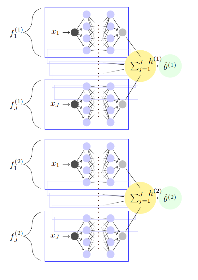
Figure 1: The network structure of a simple NAMLSS model. Each input variable as well as each distributional parameter is handled by a different neural network. $h^{(k)}$ are different activation functions depending on the distributional parameter that is modelled. E.g. a quadratic transformation for modelling the variance in a normally distributed variable to ensure the non-negativity constraint. The presented structure demonstrates a NAMLSS modelling a distribution with two parameters, e.g. a normal distribution.

We propose two different network architectures that can both flexibly model all distributional parameters. The first is depicted in Figure 1 and creates $J$ subnetworks for each of the $K$ distributional parameters. Each distributional subnetwork is comprised of the sum of the parameter-feature networks $f_{j}^{(k)}$. Hence we create $K\times J$ parameter-feature networks. To account for distributional restrictions, each distributional subnetwork is specified with possibly differing activation functions in the output layer. The second model architecture, possible due to the flexibility of neural networks, leverages the architecture of NAMs (see formula (1)) and is depicted in figure 5 in the Appendix. Here, only $J$ subnetworks are created, with each subnetwork having a $K$-dimensional output layer. This architecture thus creates the same number of subnetworks as a common NAM. Each distributional parameter, $\theta^{(k)}$, is subsequently obtained by summing over the $k$-th output of the $J$ subnetworks. Every dimension in the output layer can be activated using different activation functions, according to parameter restrictions. This allows the capture of interaction effects between the given model parameters in each of the subnetworks.

Integrating possible feature interactions can easily be achieved in both architectures by training a fully connected MLP on the residuals after the NAMLSS has converged. Hence, again leveraging the example of a normally distributed $y$, equation (3) for that interaction part becomes:

$$-\log\left(\mathcal{L}(\tilde{\mu},\tilde{\sigma}^{2}|e)\right)$$

$$=-\left(-\frac{n}{2}\log(2\pi\tilde{\sigma}^{2})-\frac{1}{2\tilde{\sigma}^{2}}\sum_{i=1}^{n}(e_{i}-\tilde{\mu})^{2}\right),$$ (5)

where $e_{i}$ denote the residuals $y_{i}-\hat{y}_{i}$.

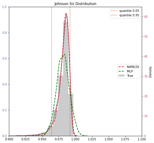
Figure 2: Johnson’s S_U Distribution: Simulated Johnson’s S_U distribution and the fit of a simple NAMLSS (see Figure 1) and a MLP. While the MLP achieves an impressive fit concerning the quadratic loss, it clearly cannot capture the underlying distribution adequately.

As neural networks can achieve optimal approximation rates, NAMLSS can learn any non-linearity or dependence between distribution parameters and features. And unlike GAMLSS, NAMLSS can model jagged shape functions and easily incorporate huge amounts of data.

Table 1: Results for Synthetic data: The benchmark results for the simulated data. We compare the models based on log-likelihoods, $\ell$. A larger log-likelihood represents a better fit. Means and standard deviations of 5-fold cross validation are reported. See the Appendix A.1, for a comprehensive list of the used log-likelihoods. Note, that for distributions where only one parameter is modelled, the two proposed NAMLSS structures are identical. Hence, we report only one value for the Binomial as well as the Poisson distribution.

Model	Binomial	Poisson	Normal	Inverse Gaussian	Weibull	Johnson’s SU
GAMLSS	-397 $\pm$ (4.0)	-800 $\pm$ (19.5)	-600 $\pm$ (23.7)	-385 $\pm$ (30.4)	-625 $\pm$ (31.1)	-370 $\pm$ (13.8)
gamboostLSS1	-315 $\pm$ (7.4)	-800 $\pm$ (19.8)	-575 $\pm$ (15.6)	-366 $\pm$ (29.0)	-648 $\pm$ (22.1)	-478 $\pm$ (15.5)
DNN	-260 $\pm$ (53.7)	-802 $\pm$ (20.2)	-558 $\pm$ (16.3)	-343 $\pm$ (31.1)	-624 $\pm$ (23.6)	-285 $\pm$ (14.1)
NAMLSS2	-	-	-589 $\pm$ (15.1)	-377 $\pm$ (26.6)	-621 $\pm$ (25.3)	-326 $\pm$ (12.1)
NAMLSS3	-274 $\pm$ (27.1)	-802 $\pm$ (18.6)	-577 $\pm$ (16.8)	-362 $\pm$ (24.9)	-620 $\pm$ (25.5)	-327 $\pm$ (12.4)

• ¹ For boosting one-parametric families like the Binomial or Poisson distribution, a model-based boosting algorithm is used (Hofner et al., 2014a).
  ² With $K$ $\times 5$ subnetworks. See Table 1 for an exemplary network structure.
  ³ With 5 subnetworks and each subnetwork returning a parameter for the location and shape respectively. See Table 5 for an exemplary network structure.
  

While predicting all parameters from a distribution may not always improve predictive power, understanding the underlying data distribution is crucial in high-risk domains and can provide valuable insights about feature effects. As an example, Figure 2 illustrates the fit of our approach on data following a Johnson’s S_U distribution, including 3 features, compared to the fit of a MLP that minimizes the Mean Squared Error (MSE). The MLP has a better predictive performance with an MSE of 0.0002, however, NAMLSS is able to reflect the underlying data distribution much more accurately (as shown in Figure 2), even though it has an MSE of 0.0005.

4 Benchmarking

To demonstrate the competitiveness of the presented method, we perform several analyses. We compare the performance of NAMLSS with several state-of-the-art models including neural as well as non-neural approaches and orientate on the benchmarks performed by Agarwal et al. (2021). Additionally, we compare related methods of distribution-focused data analysis approaches that overcome the focus on relating the conditional mean of the response to features and instead target the complete conditional response distribution. We analyze multiple datasets as well as conduct experiments on synthetic data. We choose the following baselines for the comparisons:

• Multilayer Perceptron (MLP): Unrestricted fully connected deep neural network trained with either a mean squared error loss function (regression) or binary cross entropy (logistic regression).

• Gradient Boosted Trees (XGBoost): Decision tree based gradient boosting. We use the implementation provided by Chen & Guestrin (2016).

• Neural Additive Models (NAMs): Linear combination of DNNs as described in equation (1) and presented by Agarwal et al. (2021).

• Explainable Boosting Machines (EBMs): State-of-the-art Generalized Additive Models leveraging shallow boosted trees (Lou et al., 2013).

• Deep Neural Network (DNN): Similar to the Multilayer Perceptron a fully connected neural network. However, not trained to minimize the previously mentioned loss functions but to minimize the negative log-likelihood of the specified distribution. All distributional parameters are predicted.

• Generalized Additive Models for Location Scale and Shape (GAMLSS): Standard GAMLSS models using the R implementation from Rigby & Stasinopoulos (2005).

• gamboost for Location Scale and Shape (gamboostLSS): Fitting GAMLSS by employing boosting techniques as proposed by Hofner et al. (2014b).

We preprocess all used datasets exactly as done by Agarwal et al. (2021). We perform 5-fold cross-validation for all datasets and report the average performances over all folds as well as the standard deviations. For reproducibility, we have only chosen publicly available datasets. The datasets, as well as the preprocessing and the seeds set for obtaining the folds, are described in detail in the Appendix, C. We fit all models without an intercept and explicitly do not model feature interaction effects.

4.1 Beyond the mean: Synthetic data comparison study

The synthetic data used for this task is generated from the same underlying processes. Five features are included in each application. The data-generating functions used to generate the true underlying distributional parameters can be found in Appendix C.1. Each of the five input vectors $x_{j}$ is sampled from a uniform distribution $\mathcal{U}(0,1)$, with a total of $n=3000$ observations per data set. The remaining parameters are generated based on the input vectors and the chosen distribution. We selected distributions that are widely used, popular in science, or relatively complex to reflect a diverse range of scenarios. We compare models that specifically model all distributional parameters in this simulation study. The results can be found in Table 1.

We find that the presented NAMLSS perform similarly to fully connected DNNs that specifically minimize the log-likelihood and perform better than GAMLSS or gamboostLSS, all while maintaining visual intelligibility. We can hence confirm the findings from Agarwal et al. (2021) that additive neural networks can achieve similar results to fully connected DNNs.

4.2 Experiments with Real World Data

Table 2: Benchmark results for the regression comparison datasets: For models not explicitly modelling a shape parameter, the shape is approximated with a constant as the true standard deviation of the dependent variable. Higher log-likelihoods ($\ell$) and lower MSEs are better. We report results on two commonly used regression datasets. The California Housing dataset for predicting house prices (Pace & Barry, 1997a) and an Insurance dataset for predicting billed medical expenses (Lantz, 2019).

	CA Housing		Insurance
Model	$\ell$ ($\uparrow$)	MSE ($\downarrow$)	$\ell$ ($\uparrow$)	MSE ($\downarrow$)
MLP	-4191 $\pm$(41.7)	0.197 $\pm$ (0.005)	-266.8 $\pm$ (10.9)	0.163 $\pm$ (0.022)
XGBoost	-4219 $\pm$(39.7)	0.211 $\pm$(0.005)	-266.8 $\pm$ (9.2)	0.161 $\pm$ (0.014)
NAM	-8344 $\pm$(1764.4)	0.273 $\pm$(0.037)	-474.7 $\pm$ (72.5)	0.249 $\pm$ (0.029)
EBM	-4202 $\pm$(42.2)	0.203 $\pm$(0.004)	-263.8 $\pm$ (10.1)	0.139 $\pm$ (0.017)
DNN	-2681 $\pm$(1279)	0.197 $\pm$ (0.005)	-178.2 $\pm$ (29.6)	0.165 $\pm$ (0.026)
GAMLSS	-3512 $\pm$(66.7)	0.390 $\pm$(0.035)	-175.5 $\pm$ (28.3)	0.269 $\pm$ (0.050)
gamboostLSS	-3812 $\pm$(51.7)	0.415 $\pm$ (0.026)	-141.4 $\pm$ (31.2)	0.268 $\pm$ (0.050)
NAMLSS1	-2667 $\pm$ (91.4)	0.245 $\pm$ (0.004)	-172.7 $\pm$ (22.6)	0.268 $\pm$ (0.043)
NAMLSS2	-2329 $\pm$ (176.2)	0.265 $\pm$ (0.005)	-172.6 $\pm$ (19.5)	0.265 $\pm$ (0.040)

• ¹ With $J\times K$ subnetworks. See Table 1 for an exemplary network structure.
  ² With $J$ subnetworks and each subnetwork returning a parameter for the location and shape respectively. See Table 5 for an exemplary network structure.
  

Normal Distribution

For a regression benchmark, we use the California Housing (CA Housing) dataset (Pace & Barry, 1997a) from sklearn (Pedregosa et al., 2011b) and the Insurance dataset (Lantz, 2019) and standard normalize the response variables. As comparison metrics we use the log-likelihood, $\ell$ (see Appendix, A.1), as well as the mean squared error (MSE). A larger log-likelihood thus represents a better model fit, while a smaller mean squared error represents a better predictive performance in terms of the mean. Thus, we try to illustrate the trade-off between pure predictive performance, interpretability and overall data fit.

Table 2 presents the results obtained from the analyses carried out on the two popular regression data benchmark datasets. In both applications, a normal distribution $\mathcal{N}\left(\mu,\sigma^{2}\mathcal{I}\right)$ of the underlying response variable was assumed. As the log-likelihood of a normal distribution (see equation (A.1)) is dependent on two parameters, but models as an MLP or XGBoost only predict a single parameter, we adjust the computation accordingly and use the standard deviation calculated from the underlying data for XGBoost, EBM, NAM and MLP. For NAMLSS, independent of the implementation, we use a Softplus activation for the scale parameter $\sigma^{2}$ to ensure non-negativity and a linear activation for the mean $\mu$. The NAMLSS approach achieves the highest log-likelihood values of all presented approaches which speaks for its good approximation capabilities for the California Housing dataset. It can also be seen that the trade-off between MSE performance and the possibility of modelling the response distribution is relatively moderate in its impact as NAMLSS even outperforms the predictive performance of a NAM. The results could have been further improved by accounting for feature interactions, resulting in a log-likelihood of -1654 and an MSE of 0.20.

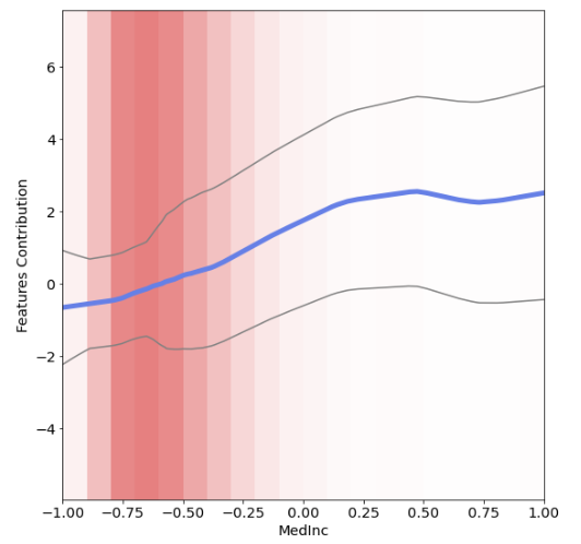
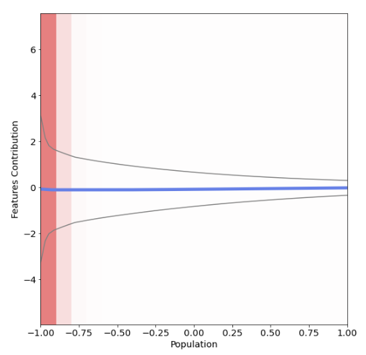
Figure 3: California Housing: Graphs for median income and population respectively learned by the NAMLSS model. We see an increase in housing prices with a larger median income. Additionally, we find a larger variance in housing prices in less densely populated areas.

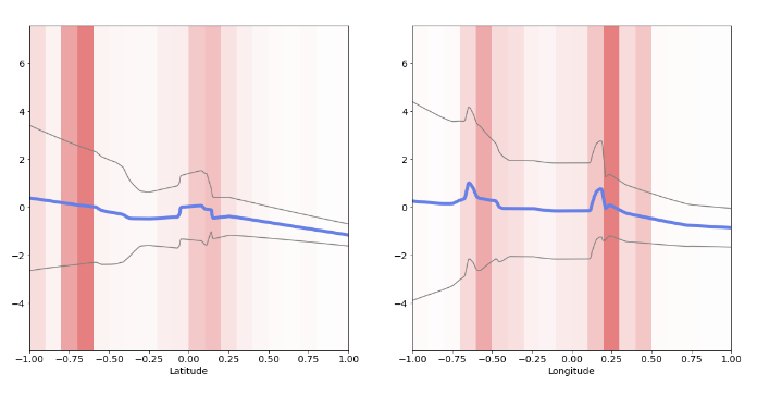
Figure 4: California Housing: Graphs for longitude and latitude respectively learned by the NAMLSS model. The house price jumps around the location of Los Angeles are depictable. Additionally, we find a decrease in variance for areas further away from the large cities.

One of the advantages of NAMLSS compared to DNNs is the feature level interpretability. Similar to NAMs, we can plot and visually analyze the results (see Figures 3 and 4). Additionally, we are able to accurately depict shifts in variance in the underlying data. It is, for example, clearly distinguishable, that with a larger median income, the house prices tend to vary much stronger than with a smaller median income (see Figure 3). A piece of information, that is lost in the models focusing solely on mean predictions. Additionally, we are capable of accurately representing sharp price jumps around the location of San Francisco, depicted by the jumps in the graphs for longitude and latitude (see Figure 4) as compared to GAMLSS, NAMLSS are additionally capable of representing jagged shape functions.

For the Insurance dataset, which is only comprised of 1338 observations, we unsurprisingly find strong performances of the classical statistical models. NAMLSS perform similarly to NAMs in terms of pure predictive power and perform similarly to DNNs in terms of log-likelihoods.

Inverse Gamma

Table 3: Benchmark results for the AirBnB dataset: For models not explicitly modelling the distributional parameters, transformations are performed. Similar for models resulting in distributional parameters but not mean predictions. A larger log-likelihood, $\ell$, and smaller average gamma deviance (see Appendix A.2) are better.

	AirBnB
Model	$\ell$ ($\uparrow$)	Avg. Gamma Dev. ($\downarrow$)
MLP	-6827 $\pm$ (177.8)	0.55 $\pm$ (0.04)
XGBoost	-5618 $\pm$ (152.4)	0.48 $\pm$ (0.09)
NAM	-5892 $\pm$ (37.0)	0.72 $\pm$(0.10)
EBM	-5474 $\pm$ (56.2)	0.49 $\pm$(0.09)
DNN	-5555 $\pm$ (33.6)	0.69 $\pm$ (0.04)
GAMLSS	-5419 $\pm$ (60.6)	0.71 $\pm$ (0.44)
gamboostLSS	-5421 $\pm$ (33.1)	0.54 $\pm$ (0.07)
NAMLSS1	-5383 $\pm$ (23.7)	0.59 $\pm$ (0.09)
NAMLSS2	-5422 $\pm$ (22.0)	0.59 $\pm$ (0.10)

• ¹ With $J\times k$ subnetworks. See Table 1 for an exemplary network structure.
  ² With $J$ subnetworks and each subnetwork returning a parameter for the location and shape respectively. See Table 5 for an exemplary network structure.
  

For the AirBnB dataset, also analyzed by Rügamer et al. (2020), we assume an Inverse Gamma distribution $\mathcal{IG}(\alpha,\beta)$ as the underlying data distribution (see equation (A.1) for the log-likelihood). For NAMLSS as well as the DNN we have to adjust the activation functions, as both models minimize the log-likelihood via the parameters $\alpha$ and $\beta$. However, the mean prediction resulting from these parameters is defined via:

$$\mu=\frac{\beta}{\alpha-1}$$

and is hence only defined for $\alpha>1$. The activation functions thus need to ensure an $\alpha$ prediction that is larger than 1 and a $\beta$ prediction that is larger than 0. Hence we again use a Softplus activation for the $\beta$ output layer. For the $\alpha$ prediction, we use the following activation function element-wise:

$$h(x)=\begin{cases}\log(1+\exp(x)),&\text{if }\log(1+\exp(x))>1,\\ \frac{1}{\log(1+\exp(x))},&\text{else}.\end{cases}$$ (6)

To compute the log-likelihood for the models resulting in a mean prediction we compute the parameters $\alpha$ and $\beta$ as follows:

$$\alpha=\frac{\mu^{2}}{\sigma^{2}+2},$$

$$\beta=\mu\frac{\mu^{2}}{\sigma^{2}+1},$$

with $\sigma^{2}$ denoting the variance of the mean predictions. For XGBoost and EBM we use a simple transformation of the target variable to ensure that $\mu>0$. Hence we fit the model on $\log(y)$ and re-transform the predictions accordingly with $\exp(\hat{y})$. Interestingly, the NAM did not converge using the Softplus activation function as the MLP did. Using the Softplus activation resulted in tremendously large mean gamma deviances and log-likelihoods, as the model kept predicting values that were nearly zero. Hence, we were only able to achieve good results for the NAM using the activation function given by formula (6).

Logistic Distribution

For a (binary) classification benchmark we use the FICO dataset (FICO, 2018). A logistic distribution, $\mathcal{LO}\left(\mu,s\right)$, of the underlying response variable was assumed (see equation (A.1) for the log-likelihood). Again, we use the true standard deviation of the underlying data for the models only resulting in a mean prediction. For evaluating the sole predictive performance we use the Area Under the Curve (AUC). The models resulting in a mean prediction use binary cross-entropy as the loss function and hence a sigmoid activation function on the output layer. NAMLSS outperforms all models in terms of log-likelihood and maintains a reasonable predictive performance, comparable to NAMs, XGBoost and EBMs (see Table 4).

Table 4: Benchmark results for the FICO dataset: For all models, modelling distributional parameters, a logistic distribution is assumed. For all other models, the binary cross-entropy loss function is minimized during training and the distributional parameters for computing the log-likelihood, $\ell$, are approximated. The Area under the Curve (AUC) (see Appendix A.2) is used.

	FICO
Model	$\ell$ ($\uparrow$)	AUC ($\uparrow$)
MLP	-1813 $\pm$(6.3)	0.79 $\pm$ (0.007)
XGBoost	-1976 $\pm$(13.4)	0.73 $\pm$(0.010)
NAM	-1809 $\pm$ (7.6)	0.73 $\pm$(0.010)
EBM	-1944 $\pm$(20.6)	0.73 $\pm$(0.010)
DNN	-1230 $\pm$ (47.5)	0.72 $\pm$ (0.006)
GAMLSS	-1321 $\pm$ (30.0)	0.78 $\pm$ (0.009)
gamboostLSS	-1191 $\pm$ (29.7)	0.79 $\pm$ (0.008)
NAMLSS1	-1201 $\pm$ (40.9)	0.73 $\pm$ (0.010)
NAMLSS2	-1160 $\pm$ (48.8)	0.72 $\pm$ (0.008)

• ¹ With $J\times k$ subnetworks. See Table 1 for an exemplary network structure.
  ² With $J$ subnetworks and each subnetwork returning a parameter for the location and shape respectively. See Table 5 for an exemplary network structure.
  

5 Conclusion & Future Work

We have presented Neural Additive Models for Location, Scale and Shape and their theoretical foundation as the neural counterpart to GAMLSS. NAMLSS can model an arbitrary number of parameters of the underlying data distribution while preserving the predictive quality of NAMs. The visual intelligibility achieved by NAMs is also maintained by NAMLSS, with the added benefit of gaining further insights from knowledge of additional distribution characteristics. Hence, NAMLSS are a further step in the direction of fully interpretable neural networks and already offer interpretability that may make them suitable for high-risk domains.

The extensibility of NAMLSS offers many different further applied and theoretical research directions. One important point is the extension of the modelling of the distribution of the response variable. Many empirical works focus on modelling not just one, but several responses conditionally on covariates. One way to do this is to use copula methods, which are a valuable extension of our approach, hence including a copula-based approach for NAMLSS models would greatly improve the overall general usefulness. Another possible extension would be the adaptation to mixture density networks, as e.g. done by Seifert et al. (2022).

Another possible focus is to switch our approach to a Bayesian-based training approach. Bayesian approaches are particularly well suited to deal with epistemic uncertainty and to incorporate it into the modelling. Another advantage is that Bayesian approaches are particularly suitable in cases where insufficiently small training datasets have to be dealt with and have been shown to have better prediction performance in these cases.

Finally, there should be a focus on incorporating unstructured data to extend the previously purely tabular data with high-dimensional input structures.

Appendix A APPENDIX

A.1 Log-Likelihoods

As the presented method minimizes negative log-likelihoods, we created a comprehensive list of all the log-likelihoods of the distributions used in the paper. When we reference the results of NAMLSS these are the log-likelihoods we used for fitting the models as well as evaluating them.

(Bernoulli) Logistic Distribution

The log-likelihood function for a logistic distribution is given by:

$$\log\left(\mathcal{L}(\mu,\sigma|y)\right)=\sum_{i=1}^{n}\left[y_{i}\log(\frac{1}{1+e^{-(\frac{y_{i}-\mu}{\sigma})}})+(1-y_{i})\log(1-\frac{1}{1+e^{-(\frac{y_{i}-\mu}{\sigma})}})\right],$$

with $n$ is as the number of observations and the parameters location $\mu\in\mathbb{R}$, scale $\sigma\in\mathbb{R}^{+}$ and $x\in\mathbb{R}$.

Binomial Distribution

The log-likelihood function for a binomial distribution is given by:

$$\log\left(\mathcal{L}(k|n,p)\right)=k\log(p)+(n-k)\log(1-p)+\log\left(\binom{n}{k}\right),$$

where $n$ is the number of trials, the parameters success probability is given by $p\in\left[0,1\right]$ and the number of successes is denoted as $k\in\mathbb{N}_{0}$.

Inverse Gamma Distribution

The log-likelihood function of the invers gamma distribution is defined as:

$$\log\left(\mathcal{L}(\alpha,\beta|y)\right)=-n\left(\alpha+1\right)\overline{\log\bm{y}}-n\log\Gamma(\alpha)+n\alpha\log\beta-\sum_{i=1}^{n}\beta y_{i}^{-1}.$$

with $\alpha>0$ and $\beta>0$ and where the upper bar operand indicates the arithmetic mean

Normal Distribution

The log-likelihood function for a normal distribution is given by:

$$log\left(\mathcal{L}(\mu,\sigma^{2}|y)\right)=-\frac{n}{2}\log(2\pi\sigma^{2})-\frac{1}{2\sigma^{2}}\sum_{i=1}^{n}(y_{i}-\mu)^{2},$$

where $n$ is the underlying number of observations and parameters $y\in\mathbb{R}$, location $\mu\in\mathbb{R}$ and scale $\sigma\in\mathbb{R}^{+}$.

Inverse Gaussian Distribution

The log-likelihood function of the inverse Gaussian distribution is given by:

$$\log\left(\mathcal{L}(\mu,\sigma|x)\right)=\frac{n}{2}\ln(\sigma)-\sum_{i=1}^{n}\frac{\sigma(x_{i}-\mu)^{2}}{2\mu^{2}x_{i}},$$

with $n$ is as the number of observations and the parameters location $\mu\in\mathbb{R}^{+}$, scale $\sigma\in\mathbb{R}^{+}$ and $x\in\mathbb{R}^{+}$.

Johnson’s S_U

The log-likelihood function of the Johnson’s S_U distribution is defined as:

$$\log\left(\mathcal{L}(\beta,\omega,\mu,\sigma|y)\right)=n\log\left[\frac{\beta}{\omega\sqrt{2\pi}}\right]-\frac{\beta^{2}}{2\omega^{2}}\sum_{i=1}^{n}\left[\frac{(y_{i}-\mu)^{2}}{\sigma^{2}}+\ln\left(1+\frac{(y_{i}-\mu)^{2}}{\omega^{2}\sigma^{2}}\right)\right],$$

with $n$ is as the number of observations and the parameters location $\mu\in\mathbb{R}$, scale $\sigma\in\mathbb{R}^{+}$, shape $\omega\in\mathbb{R}^{+}$, skewness $\beta\in\mathbb{R}$ and $y\in\mathbb{R}$.

Weibull

The log-likelihood function of the Weibull distribution is defined as:

$$\log\left(\mathcal{L}(\lambda,\beta,|y)\right)=n\ln\beta-n\beta\ln\lambda-\sum_{i=1}^{n}\left(\frac{y_{i}}{\lambda}\right)^{\beta}+(\beta-1)\sum_{i=1}^{n}\ln y_{i},$$

with $n$ is the number of observations and with the location $\lambda\in\mathbb{R}^{+}$, the shape $\beta\in\mathbb{R}^{+}$ and $y\in\mathbb{R}^{+}$.

A.2 Deviance Measures

We use several deviance measures, to evaluate the model performances beyond the log-likelihoods. These deviance measures are focused on the mere predictive power of the models. The depiction of both, the log-likelihoods as well as these deviance measures, thus captures the trade-off between pure predictive power and the ability to capture the underlying data distribution.

Mean Squared Error

The mean squared error is defined as :

$$MSE=\frac{1}{n}\sum_{i=1}^{n}(y_{i}-\hat{y}_{i})^{2}.$$

Mean Gamma Deviance

The mean gamma deviance used for the AirBnB dataset is defined as:

$$D=\frac{2}{n}\sum_{i=1}^{n}\left(\log(\frac{\hat{y}_{i})}{y_{i}})+\frac{y_{i}}{\hat{y}_{i}}-1\right).$$

Area Under the Curve

We use the Riemannian formula for the AUC. Hence the area of rectangles is defined as:

$$AR=\sum_{i}=1^{n-1}f(x_{i})\Delta x,$$

and hence with larger n, the definite integral of $f$ from $a$ to $b$ is defined as:

$$\int_{a}^{b}f(x)dx=\lim_{n\to\infty}\sum_{i=0}^{n-1}f(x_{i})\Delta x.$$

Appendix B Network architecture

We propose two different network architectures that can both flexibly model all distributional parameters. The first one is depicted in Figure 1 and creates J subnetworks for each distributional parameter. Each distributional subnetwork is comprised of the sum of $f_{j}^{(k)}$. Hence we create $K\times J$ subnetworks. To account for distributional restrictions, each distributional subnetwork is specified with possibly differing activation functions in the output layer.

The second model architecture is depicted in Figure 5. Here we only create $J$ subnetworks and hence have the same amount of subnetworks as a common NAM. Each subnetwork then has a $k$-dimensional output layer. Each distributional Parameter, $\theta^{(k)}$, is subsequently obtained by summing over the $k$-th output of the $J$ subnetworks. Each dimension in the output layer can be activated using different activation functions, adjusting to parameter restrictions.

Figure 5: The network structure of a simple NAMLSS model. Each input variable as well as each distributional parameter is handled by a different neural network. $h_{k}$ are different activation functions depending on the distributional parameter that is modelled. E.g. a quadratic transformation for modelling the variance in a normally distributed variable to ensure the non-negativity constraint.

Appendix C Benchmarking

The benchmark study for used real-world datasets was performed under similar conditions. All datasets are publicly available and we describe every preprocessing step as well as all model specifications in detail in the following.

C.1 Synthetic Data Generation

For the simulation of the data, respectively their underlying distribution parameters $\theta=\left(\theta^{(1)},\theta^{(2)},\theta^{(3)},\theta^{(4)}\right)$, the following assumptions are made:

$$\theta^{(1)} =\frac{30}{13}x_{1}\left((3x_{2}+1.5)-2\sin\left(\frac{x_{3}}{2}\right)\right)^{-1}+\frac{113}{115}x_{4}+0.1x_{5},$$

$$\theta^{(2)} =\exp\left(-0.0035x_{1}+(x_{2}-0.23)^{2}-1.42x_{3}\right)+0.0001x_{4},$$

$$\theta^{(3)} =\frac{1}{42}(4x_{1}-90x_{2}),$$

$$\theta^{(4)} =exp\left(0.0323*x_{2}+0.0123-0.0234*x_{4}\right),$$

where each of the five input vectors $x_{j}$ is sampled from a uniform distribution $\mathcal{U}(0,1)$, with a total of $n=3000$ observations per data set.

C.2 Preprocessing

We implement the same preprocessing for all used datasets and only slightly adapt the preprocessing of the target variable for the two regression problems, California Housing and Insurance. We closely follow Gorishniy et al. (2021) in their preprocessing steps and use the preprocessing also implemented by Agarwal et al. (2021). Hence all numerical variables are scaled between -1 and 1, all categorical features are one-hot encoded. In contrast to Gorishniy et al. (2021) we do not implement quantile smoothing, as one of the biggest advantages of neural models is the capability to model jagged shape functions. We use 5-fold cross-validation and report mean results as well as the standard deviations over all datasets. For reproducibility, we use the sklearn (Pedregosa et al., 2011a) Kfold function with a random state of 101 and shuffle equal to true for all datasets. For the two regression datasets, we implement a standard normal transformation of the target variable. This results in better performances in terms of log-likelihood for all models only predicting a mean and is hence even disadvantageous for the presented NAMLSS framework.

C.3 Datasets

California Housing

Table 5: Statistics of the benchmarking datasets.

Dataset	No. Samples	No. Features	Distribution	Task
California Housing	$20640$	8	Normal $\mathcal{N}(\mu,\sigma)$	Regression
Insurance	$1338$	6	Normal $\mathcal{N}(\mu,\sigma)$	Regression
Fico	$10459$	23	Logistic $\mathcal{LO}(\mu,s)$	Classification
AirBnB	$4568$	9	Inverse Gamma $\mathcal{IG}(\alpha,\beta)$	Regression

The California Housing (CA Housing) dataset (Pace & Barry, 1997b) is a popular publicly available dataset and was obtained from sklearn (Pedregosa et al., 2011a). It is also used as a benchmark in (Agarwal et al., 2021) and Gorishniy et al. (2021) and we achieve similar results concerning the MSE for the models which were used in both publications. The dataset contains the house prices for California homes from the U.S. census in 1990. The dataset is comprised of 20640 observations and besides the logarithmic median house price of the blockwise areas as the target variable contains eight predictors. As described above, we additionally standard normalize the target variable. All other variables are preprocessed as described above.

Insurance

The Insurance dataset is another regression type dataset for predicting billed medical expenses (Lantz, 2019). The dataset is publicly available in the book Machine Learning with R by Lantz (2019). Additionally, the data is freely available on Github and Kaggle. It is a small dataset with only 1338 observations. The target variable is charges, which represents the Individual medical costs billed by health insurance. Similar to the California Housing regression we standard normalize the response. Additionally, the dataset includes 6 feature variables. They are preprocessed as described above, which, due to one-hot encoding leads to a feature matrix with 9 columns.

FICO

Similar to Agarwal et al. (2021) we also use the FICO dataset for our benchmarking study. However, we use it as described on the website and hence use the Risk Performance as the target variable. A detailed description of the features and their meaning is available at the Explainable Machine Learning Challenge. The dataset is comprised of 10459 observations. We did not implement any preprocessing steps for the target variable.

AirBnB

For the AirBnB data, we orientate on Rügamer et al. (2020) and used the data for the city of Munich. The dataset is also publicly available and was taken from Inside AirBnB on January 15, 2023. After excluding the variables ID, Name, Host ID, Host Name, Last Review and after removing rows with missing values the dataset contains 4568 observations. Additionally, we drop the Neighbourhood variable as firstly the predictive power of that variable is limited at best and secondly not to create too large feature matrices for GAMLSS. Hence, in addition to the target variable, the dataset contains 9 variables. All preprocessing steps are subsequently performed as described above and the target variable, Price, is not preprocessed at all.

C.4 Model Architectures & Hyperparameters

As we do not implement extensive hyperparameter tuning for the presented NAMLSS framework, we do not perform hyperparameter tuning for the comparison models. We fit all models without an intercept. However, we try to achieve the highest comparability by choosing similar modelling frameworks, network architectures and hyperparameters where possible. All neural models are hence fit with identical learning rates, batch sizes, hidden layer sizes, activation functions and regularization techniques. Through all neural models and all datasets, we use the ADAM optimizer (Kingma & Ba, 2014) with a starting learning rate of 1e-04. For the larger datasets, California Housing and FICO, we orient on Agarwal et al. (2021) and use larger batch sizes of 1024. For the smaller dataset, Insurance, we use a smaller batch size of 256 and for the AirBnB dataset we use a batch size of 512. For every dataset and for every neural model, the maximum number of epochs is set to 2000. However, we implement early stopping with a patience of 150 epochs and no model over no fold and no dataset ever trained for the full 2000 epochs. Additionally, we reduce the learning rate with a factor of 0.95 with patience of 10 epochs for all models for all datasets. We use the Rectified Linear Unit (ReLU) activation function for all hidden layers for all models:

$$h(x)=\begin{cases}0,&x<0\\ x,&\text{else}.\end{cases}$$

We also experimented with the Exponential centred hidden Unit (ExU) activation function presented by Agarwal et al. (2021) but found no improvement in model performance and even a slight deterioration for most models.

For the statistical models used from the GAMLSS and gamboostLSS frameworks, we do not optimize the model hyperparameters, as with neural networks. We use the respective default settings unless otherwise stated in the modelling descriptions included in the Appendix. We try to keep the model settings equal between all models, if applicable. All GAMLSS models use the same RS solver proposed by (Rigby & Stasinopoulos, 2005), in cases where this approach does not lead to convergence, the alternative CG solver presented by (Cole & Green, 1992) is employed. To exclude possible numerical differences, the same distributions from the GAMLSS R package are used for modelling the response distribution and calculating the log-likelihoods. gamboostLSS allows the use of different boosting approaches. Here we use the implemented boosting methods based on GAMs and GLMs and choose the model that performs better in terms of log-likelihood and the assumed loss.

California Housing

Table 6: Hyperparameters for the neural models for the California Housing dataset

Hyperparameter	NAMLSS1	NAMLSS2	DNN	MLP	NAM
Learning Rate	1e-04	1e-04	1e-04	1e-04	1e-04
Dropout	0.25	0.25	0.25	0.25	0.25
Hidden Layers	$[1000,500,$	$[1000,500,$	$[1000,500,$	$[1000,500,$	$[1000,500,$
	$100,50,25]$	$100,50,25]$	$100,50,25]$	$100,50,25]$	$100,50,25]$
LR Decay, Patience	0.95 - 10	0.95 - 10	0.95 - 10	0.95 - 10	0.95 - 10
Activation	ReLU	ReLU	ReLU	ReLU	ReLU
Output Activation	Linear, Softplus	Linear, Softplus	Linear, Softplus	Linear	Linear

• ¹ With 2 $\times 8$ subnetworks. See Table 1 for an exemplary network structure.
  ² With 8 subnetworks and each subnetwork returning a parameter for the location and shape respectively. See Table 5 for an exemplary network structure.
  

For the California Housing dataset, we orient again on Agarwal et al. (2021) and use the following hidden layer sizes for all networks: $[1000,500,100,50,25]$. The second hidden layer is followed by a 0.25 dropout layer. While subsequently the NAM and NAMLSS have much more trainable parameters than the MLP and the DNN, we find that the MLP and DNN outperform the NAM and NAMLSS in terms of mean prediction. Additionally, we encountered severe overfitting when using the same number of parameters in an MLP as in the NAM and NAMLSS implementation. For the mean predicting models, we use a one-dimensional output layer with a linear activation. For the DNN and both NAMLSS implementations, we use a linear activation over the mean prediction and a Softplus activation for the variance prediction with:

$$h(x)=\log(1+\exp(x)).$$

For the NAMLSS implementation depicted in Figure 1 we use a smaller network structure for predicting the variance with two hidden layers of sizes 50 and 25 without any form of regularization as Dürr et al. (2020) found that using smaller networks for predicting the scale parameters is sufficient. For XGBoost we use the default parameters from the Python implementation. For the Explainable Boosting machines, we increased the number of maximum epochs to the default value of 5000 but set the early stopping patience considerably lower to 10, as otherwise, the model reached far worse results compared to the other models. We additionally increased the learning rate to 0.005 compared to the learning rate used in the neural approaches as a too small learning rate resulted in bad results. Otherwise, we kept all other hyperparameters as the default values. The GAMLSS and gamboostLSS models assume a normal distribution, with a location estimator $\mu$ employing an identity link and a scale estimator $\sigma$ with a $\log$-link function. Due to numerical instabilities, we choose to use the GLM-based boosting method instead of the default GAM-based version.

Insurance

Table 7: Hyperparameters for the neural models for the Insurance dataset

Hyperparameter	NAMLSS1	NAMLSS2	DNN	MLP	NAM
Learning Rate	1e-04	1e-04	1e-04	1e-04	1e-04
Dropout	0.5	0.5	0.5	0.5	0.5
Hidden Layers	$[250,50,25]$	$[250,50,25]$	$[250,50,25]$	$[250,50,25]$	$[250,50,25]$
LR Decay, Patience	0.95 - 10	0.95 - 10	0.95 - 10	0.95 - 10	0.95 - 10
Activation	ReLU	ReLU	ReLU	ReLU	ReLU
Output Activation	Linear, Softplus	Linear, Softplus	Linear, Softplus	Linear	Linear

• ¹ With 2 $\times 9$ subnetworks. See Table 1 for an exemplary network structure.
  ² With 9 subnetworks and each subnetwork returning a parameter for the location and shape respectively. See Table 5 for an exemplary network structure.
  

As the insurance dataset is considerably smaller than the California Housing dataset we use slightly different model structures, as the model structure used for the California Housing dataset led to worse results. Hence, for all neural models, we use hidden layers of sizes $[250,50,25]$. The first layer is followed by a 0.5 dropout layer. Again, we use a simple linear activation for the models only predicting the mean and a linear and a Softplus activation for the models predicting the mean and the variance respectively. For the first NAMLSS implementation (see Figure 1) we again use a smaller network for predicting the variance with just one hidden layer with 50 neurons.

For XGBoost and EBM we use the same hyperparameter specifications as for the California Housing dataset.

The GAMLSS and gamboostLSS models assume a normal distribution, with a location estimator $\mu$ employing an identity link and a scale estimator $\sigma$ with a $\log$-link function. The boosting for location, scale and shape method employed uses the GLM based, instead of the GAM, based version.

FICO

Table 8: Hyperparameters for the neural models for the FICO dataset

Hyperparameter	NAMLSS1	NAMLSS2	DNN	MLP	NAM
Learning Rate	1e-04	1e-04	1e-04	1e-04	1e-04
Dropout	0.5	0.5	0.5	0.5	0.5
Hidden Layers	$[250,50,25]$	$[250,50,25]$	$[250,50,25]$	$[250,50,25]$	$[250,50,25]$
LR Decay, Patience	0.95 - 10	0.95 - 10	0.95 - 10	0.95 - 10	0.95 - 10
Activation	ReLU	ReLU	ReLU	ReLU	ReLU
Output Activation	Sigmoid, Softplus	Sigmoid, Softplus	Sigmoid, Softplus	Sigmoid	Sigmoid

• ¹ With 2 $\times 23$ subnetworks. See Table 1 for an exemplary network structure.
  ² With 23 subnetworks and each subnetwork returning a parameter for the location and shape respectively. See Table 5 for an exemplary network structure.
  

For the FICO dataset, we use the exact same model structure as for the Insurance dataset, as the model structures implemented for the California Housing dataset resulted in worse results. However, as it is a binary classification problem we use a Sigmoid activation for the MLP as well as the NAM. For the DNN and both NAMLSS implementations, we use a Sigmoid activation for the location and a Softplus activation for the scale. To generate the log-likelihoods for the models only predicting a mean, we again use the true standard deviation of the underlying data.

For XGBoost and EBM we had to adjust the hyperparameters in order to get results comparable to the MLP, NAM or NAMLSS. Hence, for EBM we use 10 as the maximum number of leaves, 100 early stopping rounds and again the same learning rate of 0.005.

For XGboost we use 500 estimators with a maximum depth of 15. $\eta$ is set to 0.05.

For the GAMLSS and gamboost models we use a logistic distribution to model the response distribution, where $\mu$ estimator uses identity and the $\sigma$ estimator uses a log-link function.

AirBnB

Table 9: Hyperparameters for the neural models for the AirBnB dataset

Hyperparameter	NAMLSS1	NAMLSS2	DNN	MLP	NAM
Learning Rate	1e-04	1e-04	1e-04	1e-04	1e-04
Dropout	0.5	0.5	0.5	0.5	0.5
Hidden Layers	$[512,256,50]$	$[512,256,50]$	$[512,256,50]$	$[512,256,50]$	$[512,256,50]$
LR Decay, Patience	0.95 - 10	0.95 - 10	0.95 - 10	0.95 - 10	0.95 - 10
Activation	ReLU	ReLU	ReLU	ReLU	ReLU
Output Activation	Gamma∗, Softplus	Gamma∗, Softplus	Gamma∗, Softplus	Linear	Linear

• ¹ With 2 $\times 23$ subnetworks. See Table 1 for an exemplary network structure.
  ² With 23 subnetworks and each subnetwork returning a parameter for the location and shape respectively. See Table 5 for an exemplary network structure.
  ^∗ See formula (6) for the detailed element-wise activation function.
  

We fit the AirBnB dataset, with an Inverse Gamma distribution where applicable. However, we train the models that only predict the mean with the squared error loss function. While one might suspect worse performances due to that, we find that using the squared error actually leads to much smaller gamma deviances compared to the models leveraging the Inverse Gamma distribution. Additionally, we use slightly smaller model structures than for the California Housing dataset. For all neural models, we use hidden layers of sizes $[512,256,50]$. The first hidden layer is followed by a 0.5 dropout layer. Throughout the hidden layers, we use ReLU activation functions. However, we deviate from that for the output layer activation functions. For the MLP we use a Softplus activation function for the output layer, ensuring that strictly positive values are predicted. For NAMLSS as well as the DNN we have to adjust the activation functions, as both models minimize the log-likelihood via the parameters $\alpha$ and $\beta$. However, the mean prediction resulting from these parameters is defined via:

$$\mu=\frac{\beta}{\alpha-1}$$

and is hence only defined for $\alpha>1$. The activation functions thus need to ensure a $\alpha$ prediction that is larger than 1 and a $\beta$ prediction that is larger than 0. Hence we again use a Softplus activation for the $\beta$ output layer. For the $\alpha$ prediction, we use the following activation function element-wise:

$$h(x)=\begin{cases}\log(1+\exp(x)),&\text{if }\log(1+\exp(x))>1\\ \frac{1}{\log(1+\exp(x))},&\text{else}.\end{cases}$$

To compute the log-likelihood for the models resulting in a mean prediction we compute the parameters $\alpha$ and $\beta$ as follows:

$$\alpha=\frac{\mu^{2}}{\sigma^{2}+2},$$

$$\beta=\mu\frac{\mu^{2}}{\sigma^{2}+1},$$

with $\sigma^{2}$ denoting the variance of the mean predictions.

For XGBoost and EBM we use a simple transformation of the target variable in order to ensure that $\mu>0$. Hence we fit the model on $\log(y)$ and re-transform the predictions accordingly with $\exp(\hat{y})$. Otherwise, we use the same hyperparameters as for the California Housing dataset.

Interestingly, the NAM did not converge using the Softplus activation function as the MLP did. Using the Softplus activation resulted in tremendously large mean gamma deviances and log-likelihoods, as the model kept predicting values that were nearly zero. Hence, we were only able to achieve good results for the NAM using the activation function given by formula (6).

The presented GAMLSS and gamboostLSS models assume an Inverse Gamma distribution with both $\mu$ and $\sigma$ utilizing the log-link function. It should be noted that the RS algorithm does not converge with GAMLSS, which is why CG is used.

References

- Agarwal et al. (2021) Agarwal, R., Melnick, L., Frosst, N., Zhang, X., Lengerich, B., Caruana, R., and Hinton, G. E. Neural additive models: Interpretable machine learning with neural nets. Advances in Neural Information Processing Systems, 34, 2021.
- Chang et al. (2021) Chang, C.-H., Caruana, R., and Goldenberg, A. Node-gam: Neural generalized additive model for interpretable deep learning. arXiv preprint arXiv:2106.01613, 2021.
- Chen & Ye (2022) Chen, D. and Ye, W. Generalized gloves of neural additive models: Pursuing transparent and accurate machine learning models in finance. arXiv preprint arXiv:2209.10082, 2022.
- Chen & Guestrin (2016) Chen, T. and Guestrin, C. XGBoost: A scalable tree boosting system. In Proceedings of the 22nd ACM SIGKDD International Conference on Knowledge Discovery and Data Mining, KDD ’16, pp. 785–794, New York, NY, USA, 2016. ACM. ISBN 978-1-4503-4232-2. doi: 10.1145/2939672.2939785. URL http://doi.acm.org/10.1145/2939672.2939785.
- Cole & Green (1992) Cole, T. J. and Green, P. J. Smoothing reference centile curves: the lms method and penalized likelihood. Statistics in medicine, 11(10):1305–1319, 1992.
- de Waal & du Toit (2007) de Waal, D. A. and du Toit, J. V. Generalized additive models from a neural network perspective. In Seventh IEEE International Conference on Data Mining Workshops (ICDMW 2007), pp. 265–270. IEEE, 2007.
- Dosovitskiy et al. (2020) Dosovitskiy, A., Beyer, L., Kolesnikov, A., Weissenborn, D., Zhai, X., Unterthiner, T., Dehghani, M., Minderer, M., Heigold, G., Gelly, S., et al. An image is worth 16x16 words: Transformers for image recognition at scale. arXiv preprint arXiv:2010.11929, 2020.
- Dürr et al. (2020) Dürr, O., Sick, B., and Murina, E. Probabilistic Deep Learning: With Python, Keras and TensorFlow Probability. Manning Publications, 2020.
- FICO (2018) FICO. Fico explainable machine learning challenge. 2018.
- Gorishniy et al. (2021) Gorishniy, Y., Rubachev, I., Khrulkov, V., and Babenko, A. Revisiting deep learning models for tabular data. Advances in Neural Information Processing Systems, 34, 2021.
- Hastie (2017) Hastie, T. J. Generalized additive models. In Statistical models in S, pp. 249–307. Routledge, 2017.
- Hofner et al. (2014a) Hofner, B., Mayr, A., Robinzonov, N., and Schmid, M. Model-based boosting in r: a hands-on tutorial using the r package mboost. Computational statistics, 29:3–35, 2014a.
- Hofner et al. (2014b) Hofner, B., Mayr, A., and Schmid, M. gamboostlss: An r package for model building and variable selection in the gamlss framework. arXiv preprint arXiv:1407.1774, 2014b.
- Horel & Giesecke (2020) Horel, E. and Giesecke, K. Significance tests for neural networks. Journal of Machine Learning Research, 21(227):1–29, 2020.
- Hothorn et al. (2014) Hothorn, T., Kneib, T., and Bühlmann, P. Conditional transformation models. Journal of the Royal Statistical Society: Series B (Statistical Methodology), 76(1):3–27, 2014.
- Huang et al. (2021) Huang, Y., Giledereli, B., Köksal, A., Özgür, A., and Ozkirimli, E. Balancing methods for multi-label text classification with long-tailed class distribution. arXiv preprint arXiv:2109.04712, 2021.
- Jo & Kim (2022) Jo, W. and Kim, D. Neural additive models for nowcasting. arXiv preprint arXiv:2205.10020, 2022.
- Kingma & Ba (2014) Kingma, D. P. and Ba, J. Adam: A method for stochastic optimization. arXiv preprint arXiv:1412.6980, 2014.
- Kneib et al. (2021) Kneib, T., Silbersdorff, A., and Säfken, B. Rage against the mean–a review of distributional regression approaches. Econometrics and Statistics, 2021.
- Lantz (2019) Lantz, B. Machine learning with R: expert techniques for predictive modeling. Packt publishing ltd, 2019.
- Lin et al. (2021) Lin, Y., Meng, Y., Sun, X., Han, Q., Kuang, K., Li, J., and Wu, F. Bertgcn: Transductive text classification by combining gcn and bert. arXiv preprint arXiv:2105.05727, 2021.
- Lou et al. (2013) Lou, Y., Caruana, R., Gehrke, J., and Hooker, G. Accurate intelligible models with pairwise interactions. In Proceedings of the 19th ACM SIGKDD international conference on Knowledge discovery and data mining, pp. 623–631, 2013.
- Nagrani et al. (2021) Nagrani, A., Yang, S., Arnab, A., Jansen, A., Schmid, C., and Sun, C. Attention bottlenecks for multimodal fusion. Advances in Neural Information Processing Systems, 34:14200–14213, 2021.
- Nelder & Wedderburn (1972) Nelder, J. A. and Wedderburn, R. W. Generalized linear models. Journal of the Royal Statistical Society: Series A (General), 135(3):370–384, 1972.
- Pace & Barry (1997a) Pace, R. K. and Barry, R. Sparse spatial autoregressions. Statistics & Probability Letters, 33(3):291–297, 1997a.
- Pace & Barry (1997b) Pace, R. K. and Barry, R. Sparse spatial autoregressions. Statistics & Probability Letters, 33(3):291–297, 1997b. Publisher: Elsevier.
- Pedregosa et al. (2011a) Pedregosa, F., Varoquaux, G., Gramfort, A., Michel, V., Thirion, B., Grisel, O., Blondel, M., Prettenhofer, P., Weiss, R., Dubourg, V., Vanderplas, J., Passos, A., Cournapeau, D., Brucher, M., Perrot, M., and Duchesnay, E. Scikit-learn: Machine Learning in Python. Journal of Machine Learning Research, 12:2825–2830, 2011a.
- Pedregosa et al. (2011b) Pedregosa, F., Varoquaux, G., Gramfort, A., Michel, V., Thirion, B., Grisel, O., Blondel, M., Prettenhofer, P., Weiss, R., Dubourg, V., Vanderplas, J., Passos, A., Cournapeau, D., Brucher, M., Perrot, M., and Duchesnay, E. Scikit-learn: Machine learning in Python. Journal of Machine Learning Research, 12:2825–2830, 2011b.
- Peroni et al. (2022) Peroni, M., Kurban, M., Yang, S. Y., Kim, Y. S., Kang, H. Y., and Song, J. H. Extending the neural additive model for survival analysis with ehr data. arXiv preprint arXiv:2211.07814, 2022.
- Potts (1999) Potts, W. J. Generalized additive neural networks. In Proceedings of the fifth ACM SIGKDD international conference on Knowledge discovery and data mining, pp. 194–200, 1999.
- Ribeiro et al. (2016) Ribeiro, M. T., Singh, S., and Guestrin, C. ” why should i trust you?” explaining the predictions of any classifier. In Proceedings of the 22nd ACM SIGKDD international conference on knowledge discovery and data mining, pp. 1135–1144, 2016.
- Rigby & Stasinopoulos (2005) Rigby, R. A. and Stasinopoulos, D. M. Generalized additive models for location, scale and shape. Journal of the Royal Statistical Society: Series C (Applied Statistics), 54(3):507–554, 2005.
- Rügamer et al. (2020) Rügamer, D., Kolb, C., and Klein, N. Semi-structured deep distributional regression: Combining structured additive models and deep learning. arXiv preprint arXiv:2002.05777, 2020.
- Seifert et al. (2022) Seifert, Q. E., Thielmann, A., Bergherr, E., Säfken, B., Zierk, J., Rauh, M., and Hepp, T. Penalized regression splines in mixture density networks, 2022. URL https://doi.org/10.21203/rs.3.rs-2398185/v1.
- Shapley (1953) Shapley, L. Quota solutions op n-person games1. Edited by Emil Artin and Marston Morse, pp. 343, 1953.
- Sundararajan & Najmi (2020) Sundararajan, M. and Najmi, A. The many shapley values for model explanation. In International conference on machine learning, pp. 9269–9278. PMLR, 2020.
- Wang et al. (1996) Wang, P., Puterman, M. L., Cockburn, I., and Le, N. Mixed poisson regression models with covariate dependent rates. Biometrics, pp. 381–400, 1996.
- Yang et al. (2021) Yang, Z., Zhang, A., and Sudjianto, A. Gami-net: An explainable neural network based on generalized additive models with structured interactions. Pattern Recognition, 120:108192, 2021.
- Yu et al. (2022) Yu, J., Wang, Z., Vasudevan, V., Yeung, L., Seyedhosseini, M., and Wu, Y. Coca: Contrastive captioners are image-text foundation models. arXiv preprint arXiv:2205.01917, 2022.
- Zeng et al. (2022) Zeng, A., Chen, M., Zhang, L., and Xu, Q. Are transformers effective for time series forecasting? arXiv preprint arXiv:2205.13504, 2022.
- Zhou et al. (2022) Zhou, T., Ma, Z., Wen, Q., Sun, L., Yao, T., Jin, R., et al. Film: Frequency improved legendre memory model for long-term time series forecasting. arXiv preprint arXiv:2205.08897, 2022.