Neutrinos from dense environments : Flavor mechanisms, theoretical approaches, observations, and new directions

Abstract

Neutrino masses and mixings produce vacuum oscillations, an established quantum mechanical phenomenon. In matter, the Mikheev-Smirnov-Wolfenstein effect, due to neutrino interactions with the background particles, triggers resonant flavor modification. In dense environments, such as core-collapse supernovae or compact mergers, sizable neutrino-neutrino interactions, shock waves and turbulence impact the neutrino flavor content under a variety of phenomena. Theoretical approaches of neutrino propagation range from the mean-field approximation to the full quantum kinetic equations. Intriguing connections have been uncovered between weakly interacting dense neutrino gases and other many-body systems and domains, from condensed matter and nuclear physics to quantum computing. Besides the intrinsic theoretical interest, establishing how neutrinos change flavor contributes to answer the longstanding open questions of how massive stars explode and of the $r$-process sites. It is also important for future observations of core-collapse supernova neutrinos and of the diffuse supernova neutrino background that should be discovered in the foreseeable future.

I General and historical

I.1 The birth of neutrino astronomy

In his famous letter to Lise Meitner, and to ”Dear Radioactive Ladies and Gentlemen”, Pauli [402, 403] hypothesized the existence of a new fermion, the neutron. He wanted to explain the observed continuous beta spectrum in the $\beta$-decay of atomic nuclei and ”to save the laws of energy conservation and the statistics”. This particle had to be as light as the electron with a mass not heavier than 0.01 the one of the proton. Renamed neutrino (”small neutral particle” in Italian), it remained elusive until Cowan et al. [160] detected electron anti-neutrinos via inverse $\beta$-decay from nearby reactors, the most powerful human-made neutrino sources in terrestrial experiments.

The same year Lee and Yang [322] examined the question of parity conservation in weak interactions, stimulated by the so-called $\theta$-$\tau$ meson puzzle. They suggested, as a possible experimental test of the parity non-conservation hypothesis, the measurement of a pseudo-scalar observable, namely the angular distribution of electrons emitted in polarized ⁶⁰Co decay. In a few months Wu et al. [511] successfully performed the experiment, demonstrating weak interaction differentiates the right from the left. In 1958 Goldhaber et al. [258] measured neutrinos from electron capture in ¹⁵²Eu and found them to be left-handed. In the Glashow [255], Weinberg [507], Salam [439] (GWS) model, there are three neutrino flavors, $\nu_{\_}e$, $\nu_{\_}{\mu}$ and $\nu_{\_}{\tau}$ and neutrinos are massless.

In his seminal work Bethe [97] suggested that carbon and nitrogen act as catalysts in a chain reaction and are mainly responsible for hydrogen burning into helium in luminous main sequence stars (later known as the CNO cycle). Afterwards, solar models predicted sizable $\nu_{\_}e$ fluxes from energy generation mostly due to hydrogen burning into helium in the proton-proton (pp) reaction chain [68]. It was Davis et al. [173] who first detected solar neutrinos with his pioneering radiochemical experiment in the Homestake mine, using neutrino capture on ³⁷Cl [174]. In a few months the measurement revealed less neutrinos than expected according to the predictions of [69]: the solar neutrino problem was born. Based on these observations it was deduced that only a small portion of the solar radiated energy was coming from the CNO cycle [173, 69].

For over more than three decades, radiochemical, water Cherenkov and scintillator experiments showed that, depending on neutrino energy, one-third to one-half of the predicted solar neutrino fluxes were actually reaching the Earth (see for example [423, 249, 275]). Both the Standard Solar Model and neutrino properties were questioned. Helioseismology brought an important clue in favor of the Standard Solar Model (see for example [487]). In particular, the solar sound speed, measured at a few $\%$ level, was agreeing with predictions.

Among the debated solutions of the solar neutrino problem was the possibility that neutrinos could oscillate, as earlier pointed out by Pontecorvo [412, 413] who first suggested that $\nu$ could transform into $\bar{\nu}$. Later on, Gribov and Pontecorvo [260] considered the possibility of $\nu_{\_}e$ oscillations into $\nu_{\_}{\mu}$ in analogy with oscillations of neutral $K_{\_}0$-$\bar{K}_{\_}0$ mesons.

Wolfenstein [508] pointed out that in matter neutrinos can change flavor due to coherent forward scattering and a flavor-dependent refractive index. In a subsequent work, Wolfenstein [509] explained that matter at high density in collapsing stars can inhibit vacuum oscillations. Later on, Mikheev and Smirnov [363] realized that flavor conversion in matter could be resonantly amplified: an adiabatic evolution at the resonance location could solve the solar neutrino problem (see also [363, 115, 96, 274, 398]). This phenomenon became to be known as the Mikheev-Smirnov-Wolfenstein (MSW) effect.

In 1987, the explosion of the blue supergiant Sk-69^∘202 brought evidence that core-collapse supernovae emit $\nu$ at the end of their life (Figure 1). SN1987A was in the Large Magellanic Cloud (LMC), a satellite galaxy of the Milky Way. Kamiokande-II (KII) [278], Irvine-Michigan-Brookhaven (IMB) [104] detectors and the Baksan Scintillator Telescope (BST) [41] recorded a 10 seconds burst of about 24 events, with a few tens of MeV energy. The Mont Blanc Liquid Scintillator Detector (LSD) [24] detected 5 events, five hours before others, so that the connection of LSD events to SN1987A remains controversial.

The neutrino events from SN1987A confirmed that neutrinos take away most of the gravitational energy, as Colgate and White [157] conjectured, and agreed overall with the predicted neutrino fluxes and spectra. Moreover, the Bayesian analysis of the SN1987A time signal by Loredo and Lamb [327] corroborated a two-component (accretion+cooling) model at $2$-$3\sigma$, which was confirmed by the subsequent analysis by Pagliaroli et al. [396]. This supported the delayed neutrino-heating mechanism of Bethe and Wilson [100], thus rejecting the favored prompt bounce-shock model by Colgate and White [157]. On the particle physics side, the about two dozens events brought an impressive amount of constraints on unknown neutrino properties (e.g. the neutrino magnetic moment, charge radius or decay), on non-standard interactions and particles such as axions (see for example [423, 533, 369, 404, 141, 78, 341, 217]).

The observation of neutrinos from the Sun and from SN1987A pioneered neutrino astronomy. The detection of PeV neutrinos in the IceCube detector at the South Pole [1] opened a new observational window. One of the events detected so far is consistent with blazar TXS 0506+056 [2]. Furthermore, $79^{+22}_{\_}{-20}$ TeV neutrino events have been associated to the active galaxy NGC1068 and a supermassive black hole, with a statistical significance of 4.2 $\sigma$ [12]. With these observations, neutrino astronomy now covers from MeVs to the highest neutrino energies.

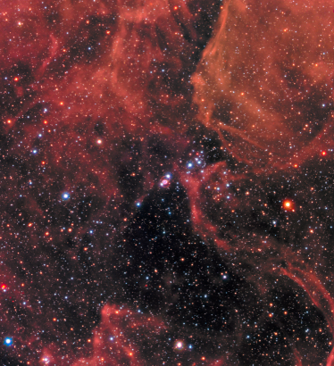
Figure 1: Hubble Space Telescope image of SN1987A, in the Large Magellanic Cloud, a neighboring galaxy of our Milky way, 30 years after its explosion. The central part of the image – SN1987A – shows three rings which correspond to earlier events. The central inner ring is material that has been ejected by the star about 20 000 years before SN1987A. The material ejected by the supernova explosion has reached the inner ring and makes it glow. (Figure from [380]).

I.2 The oscillation discovery

Primary cosmic rays interacting with the Earth’s atmosphere produce twice as many $\nu_{\_}{\mu}$ as $\nu_{\_}{e}$ from $\pi$ and $\mu$ decay. Underground experiments searching for proton instability, which was expected in some unified theories, reported a reduced $\nu_{\_}{\mu}/\nu_{\_}e$ ratio in the atmospheric background, with respect to Monte-Carlo simulations. This was known as the atmospheric anomaly (see for example 249).

In 1998 the Super-Kamiokande (Super-K) Collaboration [233] discovered that atmospheric $\nu_{\_}{\mu}$ traversing the Earth (up-going) were less than expected, whereas up-going $\nu_{\_}{e}$ stayed unaffected. The zenith angle dependence of the $\mu$-like and $e$-like events gave unambiguous proof that $\nu_{\_}{\mu}$ oscillated into $\nu_{\_}{\tau}$.

The Sudbury Neutrino Observatory (SNO) [32] and the Kamioka Liquid Scintillator Antineutrino Detector (KamLAND) [197] experiments brought two further milestones in the clarification of the solar neutrino problem. The first experiment [33], using heavy water, found ⁸B solar neutrinos to be in agreement with the Standard Solar Model predictions. The different sensitivity of $\nu_{\_}e$ and $\nu_{\_}{\mu},\nu_{\_}{\tau}$ to elastic scattering, combined with neutral- and charged-current $\nu$ interactions on deuterium allowed to identify the solar $\nu_{\_}{\mu},\nu_{\_}{\tau}$ fluxes at $5.3~{}\sigma$ [34]. Moreover KamLAND [197] measured $\bar{\nu}_{\_}e$ disappearance at an average distance of 200 km from Japanese reactors and unambiguously identified the MSW solution called large-mixing-angle (LMA). .

These observations established that only half of low energy (less than 2 MeV) solar $\nu_{\_}e$ reach the Earth because of averaged vacuum oscillations; whereas high energy ⁸B neutrinos are reduced to one-third due to the MSW effect. The solar neutrino problem was finally solved.

The solution of the solar neutrino problem had required more than three decades of searches, concerning in particular the origin of the energy dependence of the solar neutrino deficit, the day/night effect, seasonal variations, and was also the result of global data analysis and fits. These investigations excluded other explanations due to non-standard physics, investigated along the years, such as neutrino decay, non-standard interactions or the neutrino magnetic moment (see for example the review by Haxton et al. [275]).

Furthermore the Borexino experiment measured for the first time the solar ⁷Be [61], the $pep$ [94] and the $pp$ neutrinos from the keystone reaction of the $pp$ reaction chain. The corresponding fluxes are consistent with vacuum-averaged oscillations. In particular, the measurement of the ⁷Be flux brought the confirmation that the $\nu_{\_}e$ survival probability increases in the vacuum-dominated region. Besides neutrinos from the CNO cycle were first detected [27], confirming that it contributes to solar fusion at 1 $\%$ level, favoring Standard Solar models with high metallicity.

Vacuum oscillations imply that neutrinos are elementary particles with non-zero masses and mixings. Hence, the flavor and mass bases are related by the Pontecorvo-Maki-Nakagawa-Sakata (PMNS) unitary matrix, analogous to the Cabibbo-Kobayashi-Maskawa matrix in the quark sector (although with large mixing angles).

Since 1998, atmospheric, solar, reactor and accelerator experiments have determined most of the neutrino oscillation parameters in the theoretical framework with three active neutrinos. The mixing angles, $\theta_{\_}{23}\approx 45^{\circ}$, $\theta_{\_}{12}\approx 35^{\circ}$ and $\theta_{\_}{13}\approx 8.2^{\circ}$, as the mass-squared differences $\Delta m^{2}_{\_}{32}=m^{2}_{\_}{3}-m^{2}_{\_}{2}=2.4\times 10^{-3}$ eV² (atmospheric) and $\Delta m^{2}_{\_}{21}=m^{2}_{\_}{2}-m^{2}_{\_}{1}=7.5\times 10^{-5}$ eV² (solar) [533] are known with good accuracy (few percent precision). The PMNS matrix also depends on three phases, one Dirac and two Majorana phases. The Dirac phase is being measured. It can produce a difference between neutrino and antineutrino oscillations, breaking the CP symmetry (C for charge conjugation and P for parity). The Majorana phases remain unknown.

The discovery of neutrino vacuum oscillations was a breakthrough: it opened a window beyond the Standard model and had an impact in astrophysics and cosmology.

I.3 Unknown neutrino properties

Key neutrino properties remain unknown and will be the object of an intense experimental program. Sixty years after Christenson et al. [152] discovered that weak interaction breaks the CP symmetry in $K_{\_}0$ decay, there are indications that neutrinos do not oscillate in the same way as antineutrinos. If confirmed by future experiments, this will point to the presence of CP violation in the lepton sector and to CP breaking values of the Dirac phase (see for example [129] for an analysis).

The ordering of the neutrino mass eigenstates needs to be established, since the atmospheric mass-squared difference sign has not been measured yet. The neutrino mass ordering (or hierarchy) might be normal ($\Delta m^{2}_{\_}{32}>0$), or inverted ($\Delta m^{2}_{\_}{32}<0$). On the other hand, the sign of the solar mass-squared difference is determined by the presence of the MSW resonance in the Sun. Currently data show a preference (at 2.5 $\sigma$) for normal ordering, i.e. the third mass eigenstate is likely more massive than the others [129].

Vacuum oscillations are sensitive to mass-squared differences but do not give information on the scale of the neutrino masses. The absolute neutrino mass scale is not identified yet. The KATRIN experiment has obtained sub-eV upper limits ($m<0.8$ eV at 90 $\%$ confidence level) on the effective $\nu_{\_}e$ mass with tritium $\beta$-decay [36]. Complementary information comes from cosmological observations which give (model dependent) information on the sum of the neutrino masses (at sub-eV level) [533].

The ensemble of results from oscillation experiments cannot be fully interpreted in the theoretical framework with three active neutrinos. It presents some anomalies. The reactor antineutrino anomaly refers to a discrepancy, at 5-6 $\%$ level, between the predicted and measured ${\bar{\nu}}_{\_}e$ fluxes from nuclear power plants, due to a reevaluation of the fluxes [358]. The Gallium anomaly refers to a $\nu_{\_}e$ deficit observed in the solar GALLEX and SAGE experiments when the fluxes from a radioactive source were measured [251]. The last debated anomalies come from neutrino accelerator experiments, namely the LSND experiment that measured vacuum oscillations at $\Delta m^{2}\approx 1$ eV² and the MiniBooNE experiment that found an excess of $\nu_{\_}e$ events at low energy.

Recent evaluations of the reactor neutrino fluxes and a campaign of nuclear measurements have lowered the statistical significance of the reactor anomaly [252, 529], whereas the Gallium one, confirmed by the counting BEST experiment [84], gives sterile mixing parameters in tension with the reactor anomaly. Moreover, the first results from the MicroBooNE experiment [56] disfavor some explanations and part of the parameter space identified by the MiniBooNE low energy excess. Clearly further work is needed to elucidate the origin of such anomalies.

Among the debated solutions of the anomalies is the existence of a fourth non-standard sterile neutrino. Sterile neutrinos do not interact with matter (they do not couple to the Standard Model gauge bosons) and can manifest themselves in neutrino vacuum oscillations because of their coupling to active neutrinos through a PMNS matrix with $N\geq 4$. The existence of sterile neutrinos is actively debated (see for example [23]).

The origin of the neutrino masses remains an open issue. See-saw mechanisms constitute a possibility to explain the smallness of neutrino masses and are investigated in numerous theories beyond the Standard model (see for example the reviews [43, 305]). In the simplest (Type-I) see-saw models, neutrinos acquire a small mass because of the existence of very heavy right-handed neutrinos.

Moreover, as pointed out long ago by Majorana [342], neutrinos could well be their own antiparticles. Searches for a rare nuclear process called 0$\nu$2$\beta$ decay that implies total lepton-number violation [249, 26] appear the most feasible path to uncover the neutrino nature and give access to the Majorana CP violating phases. As for neutrino electromagnetic properties, such as the neutrino magnetic moment, only bounds exist (see for example [250]).

In conclusion, the key open issues in neutrino physics include the neutrino absolute mass and mass ordering, the origin of neutrino masses, the existence of CP violation in the lepton sector and of sterile neutrinos, the neutrino Dirac versus Majorana nature and neutrino electromagnetic properties.

Neutrino properties are intertwined with neutrino flavor evolution in dense sources and influence observations. Therefore, as we shall discuss, neutrinos from such environments offer ways to learn about some of the unknowns on the one hand, and constitute a unique probe in astrophysics and in cosmology on the other.

I.4 Future supernova neutrino observations

SN1987A remains to date the only core-collapse supernova observed through its neutrinos. Supernovae type II and Ib/c are exciting and a rich laboratory for particle physics and astrophysics, requiring both multipurpose and dedicated neutrino observatories that can run over long time periods.

A network of neutrino detectors, based on different technologies, around the world, is awaiting for the next (extra)galactic supernova explosion. Among the detectors included in the network are the helium and lead observatory (HALO, 76 tons of lead), KamLAND (1 kton, liquid scintillator), the deep underground neutrino experiment (DUNE, 40 ktons, liquid argon), the Jiangmen underground neutrino observatory (JUNO, 20 kton, liquid scintillator), IceCube (cubic-km, Cherenkov detector) and in the future the Hyper-Kamiokande (Hyper-K, water Cherenkov, 248 ktons) and the dark matter wimp search with liquid xenon (DARWIN, 40 tons). The Supernova Early Warning System (SNEWS) [453, 40] should alert astronomers if the lucky event of a supernova explosion takes place.

In the Milky Way the spatial probability distribution of objects that are likely to become supernovae has its maximum at the galaxy center at 8 kpc while its mean is at 10 kpc. The latter is mostly adopted to make predictions.

Neutrino observatories will measure the time signal and the spectra of $\nu_{\_}e$, $\bar{\nu}_{\_}e$, $\nu_{\_}x,\bar{\nu}_{\_}x$ ($x=\mu,\tau$) with charged-current $\nu_{\_}e$ scattering on nuclei, inverse $\beta$-decay, elastic scattering on electrons and on protons [88], and coherent neutrino-nucleus scattering [39]. If a supernova explodes in our galaxy (10 kpc), detectors will measure about 40 (540) events in HALO (HALO-2, 1 kton) [490], hundreds in KamLAND, up to $3\times 10^{3}$ in DUNE [22], up to about $8\times 10^{3}$ in JUNO [45], almost 10⁴ in Super-K [90], $10^{5}$ in Hyper-Kamiokande [19] and $10^{6}$ in IceCube. From a supernova in Andromeda galaxy (M31, 773 kpc) which has a low supernova rate, 12 events are expected in Hyper-K.

Dark matter detectors will also measure supernova neutrinos through coherent neutrino-nucleus scattering, sensitive to all neutrino flavors. Xenon nT/LZ (7 tons) and DARWIN (40 tons) will measure 120 and 700 events, and have a discovery potential for supernova neutrinos up to the Milky Way edge and the small Magellanic Cloud (SMC), respectively (27 ${\rm M}_{\_}{\odot}$ progenitor) [318]. For the same progenitor, a liquid argon dark matter detector such as Darkside-20k (50 tons) will detect 336 events (supernova at 10 kpc) and be able to detect supernova neutrinos up to the LMC; whereas Argo (360 tons) will detect 2592 events and be sensitive to a supernova explosion up to the SMC [25].

Supernovae are rare in our galaxy. Typical quoted number for the core-collapse supernova rate in our Galaxy is 1-3/century. Rozwadowska et al. [435], obtained a mean time of occurrence of 61 ${}^{+24}_{\_}{-14}$ based on neutrino and electromagnetic observations of collapse events in the Milky Way and the Local Group.

Supernovae are frequent in the universe. With a 1 Mt detector, about one supernova per year is expected within 10 Mpc, due to nearby galaxies with higher rates than the Milky Way. Within 4 Mpc, less than one neutrino event per year would be detected [53].

Neutrinos from past supernova explosions form a relic, or diffuse, supernova neutrino background (DSNB) (see the reviews by Ando and Sato [55], Beacom [87], Lunardini [334], Mathews et al. [354], Suliga [469], Ando et al. [54]). Its flux, integrated over cosmological redshift, depends on the redshifted supernova neutrino fluxes, on the evolving core-collapse supernova rate and on the fraction of failed supernovae that turn into a black hole without an electromagnetic counterpart [333, 300]. At present we only have upper limits.

Super-K [343] set the first upper limit of $1.2$ $\bar{\nu}_{\_}e$ cm^-2s^-1 ($E_{\_}{\nu}>19.3~{}$MeV, 90 $\%$ CL) on the supernova relic flux. The bound was improved with Super-K IV data [530] using $\bar{\nu}_{\_}e$ detection via inverse $\beta$-decay and neutron tagging on protons. The DSNB search combining Super-K I to Super-K IV data yields $2.7$ $\bar{\nu}_{\_}e$ cm^-2s^-1 ($E_{\_}{\nu}>17.3~{}$MeV, 90 $\%$ CL). The KamLAND experiment obtained the upper value of 139 $\bar{\nu}_{\_}e$ cm^-2s^-1 (90 $\%$ CL) in the window $[8.3,31.8]$ MeV [242]. The Borexino Collaboration extracted a model dependent limit of 112.3 $\bar{\nu}_{\_}e$ cm^-2s^-1 (90 $\%$ CL) in the interval $[7.8,16.8]$ MeV [28].

As for $\nu_{\_}e$, the ensemble of SNO data provided the upper limit of 19 $\nu_{\_}e$ cm^-2s^-1 in the window $[22.9,36.9]$ MeV (90 $\%$ CL) [29]. The loosest limits are $\phi_{\_}{\nu_{\_}x,\bar{\nu}_{\_}x}<$ 1.3-1.8 10³ cm^-2s^-1 ($E_{\_}{\nu}>19$ MeV) [335] (for $x=\mu,\tau$ flavors). With neutrino-nucleus coherent scattering in dark matter detectors, one could improve this bound to 10 $\nu_{\_}x$ or $\bar{\nu}_{\_}x$ [470].

Beacom and Vagins [89] suggested to add gadolinium (Gd) to water Cherenkov detectors. Neutron capture by Gd improves inverse $\beta$-decay tagging through the 8 MeV photons following the capture. The SK-Gd experiment is currently taking data.

DSNB predictions are close to current bounds (see [55, 234, 332, 525, 237, 135, 494, 415, 286, 368, 312, 288, 475, 175, 199, 63, 64]). The analysis from the combined SK-I to IV data shows an excess at 1.5 $\sigma$ over background prediction [20]. The related sensitivity analysis is on par with four of the most optimistic predictions [55, 283, 312, 237] and a factor of about 2-5 larger than the most conservative ones. With SK-Gd, the upcoming JUNO, the more distant future Hyper-K and DUNE experiments, the DNSB should be discovered in the forthcoming future. And indeed, its discovery could be imminent.

I.5 The $r$-process and GW170817

Besides direct observations of neutrinos from supernovae, the study of indirect effects produced by neutrinos in dense environments has also stimulated intense investigations of neutrinos and of neutrino flavor evolution in dense media. Neutrinos in dense environments are tightly connected to two unresolved issues in astrophysics: the death of massive stars and the origin of $r$-process elements ($r$-process stands for rapid neutron capture process).

Currently, two- and three-dimensional simulations include realistic neutrino transport, convection, turbulence and hydrodynamical instabilities such as the standing accretion-shock instability (SASI) [108] and the lepton-number emission self-sustained asymmetry (LESA) [478] (see for example Kotake et al. [311], Janka [290, 291], Mezzacappa et al. [361], Radice et al. [419], Burrows et al. [122], Takiwaki et al. [477], Foglizzo et al. [224]). The delayed neutrino-heating mechanism is believed to trigger most of core-collapse supernova explosions. The most energetic supernovae might require a magneto-hydrodynamical mechanism (see for example Janka [290]). The future observation of neutrinos from a galactic or extragalactic supernova could confirm or refute the current paradigm and elucidate a six-decade quest.

The $r$-process is a nucleosynthesis process which takes place in a neutron-rich environment and during short timescales (i.e. seconds). In this process nuclei capture neutrons faster than they undergo $\beta$-decay towards the stability line. The $r$-process produces thousands of exotic nuclei far from the neutron drip-line and about half of the heavy elements in our galaxy. A weak $r$-process produces elements in the first peak around mass number A=80-90 and the second peak around A=130-138. A strong $r$-process reaches the third peak at A=195-208.

Burbidge et al. [118] and Cameron [125] first linked the $r$-process to core-collapse supernovae which have long been thought the main $r$-process site (see for example Qian [416], Kajino et al. [297]). While simulations show that entropies are typically too low, the most energetic supernovae seem to provide the right conditions to attain a successful nucleosynthesis (see Côté et al. [163], Cowan et al. [161] for a comprehensive review).

Another candidate site for the $r$-process are binary neutron star mergers (BNS) as first suggested by Lattimer and Schramm [320, 321] (see for example [297, 163, 259] for reviews). As supernovae, BNS are powerful sources of MeV neutrinos. Indeed they emit 10⁵¹ to 10⁵³ erg in $\nu_{\_}e$, ${\nu}_{\_}{\mu}$, ${\nu}_{\_}{\tau}$ and their antiparticles, with tens of MeV. Contrary to supernovae, binary neutron star mergers are more neutron-rich and produce an excess of $\bar{\nu}_{\_}e$ over $\nu_{\_}e$ (see e.g. Cusinato et al. [162]). As for ${\nu}_{\_}{\mu}$s and ${\nu}_{\_}{\tau}$s, their fluxes are predicted to be small compared to those of core-collapse supernovae and have large theoretical uncertainties. If supernovae are more frequent than BNS, simulations show that BNS offer more suitable astrophysical conditions for a strong $r$-process. Moreover studies have shown some $r$-process elements are synthetised in accretion disks around black holes [472] and black hole-neutron star mergers [473, 123].

The first detection of gravitational waves from the fusion of two black-holes by the Virgo-LIGO Collaboration [13] has opened the era of gravitational wave astronomy. To date, GW170817 [15, 14] is a unique multi-messenger event in which gravitational waves from a binary neutron star merger were first detected, also concomitantly with a short-gamma ray burst and a kilonova. The electromagnetic signal of a kilonova [359], or macronova [313] is in-between the ones of novae and supernovae. Since the afterglow emission of the kilonova associated with GW170817 extends over some days, it appears that radioactivity injects some energy, powering the kilonova. The optical/IR spectra in the IR emission peak are compatible with elements heavier than iron to be responsible for absorption and reemission of the radiation [161] (Fig. 2). In particular, the ejecta opacities show presence of actinides and lanthanides (see for example the studies by [163, 483, 161]). This represents the first evidence for $r$-process elements in binary neutron star mergers.

Before GW170817 dynamical ejecta were thought to mainly contribute to a strong $r$-process (see for example the discussion in Martin et al. [349]. But, the kilonova observation has changed this paradigm. Indeed the comparison of the electromagnetic emission with most models shows two components: the early and fast pre-merger contribution from dynamical ejecta, the later post-merger one due to viscosity and neutrino-driven winds. The former is associated with red emission, the latter with the blue one [420]. The role of neutrinos on the pre- and post-merger ejecta and of flavor evolution appears crucial and is currently object of debate (see e.g. Nedora et al. [381]).

Indeed numerous $r$-process studies include not only neutrinos but also neutrino flavor evolution. Many find that matter becomes proton-rich and tends to harm the $r$-process in core-collapse supernovae. One should keep in mind though the complexity of studying flavor evolution in dense environments in a consistent manner tracking the evolution both of the neutrino flavor and of the nucleosynthetic abundances. This is true both for core-collapse supernovae and for BNS. Depending on the site and on the assumptions made, one can find situations in which flavor modification favors, or harms, the $r$-process. In general, what emerges from investigations is that neutrino flavor evolution impacts the nucleosynthetic abundances when one includes standard or non-standard $\nu$ properties and interactions.

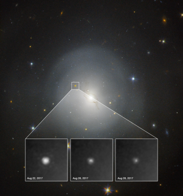
Figure 2: Hubble Space Telescope image of kilonova gradually fading, in the lenticular galaxy NGC 4993 (40 Mpc). The event GW170817 was seen concomitantly in gravitational waves, in electromagnetic emission and with a short gamma-ray burst. It represents the first observation from merging binary neutron stars. (Figure adapted from [379]).

In conclusion, the quest for the identification of the $r$-process site(s) and the supernova mechanism as well as the need of predictions for future observations has motivated an in-depth investigation of flavor evolution in dense environments for many years, as we shall now discuss.

I.6 Theoretical developments

In an astrophysical environment such as binary neutron star merger remnants or core-collapse supernovae, the environments are not only dense in matter but also in neutrinos. Indeed, in such sites the neutrino density becomes comparable to the one of electrons or of nucleons. For example, during the explosion of a core-collapse supernova, about $10^{58}\nu$ with an average energy of 10 MeV are emitted, so that the neutral-current $\nu\nu$ interaction becomes sizable.

Undoubtedly, understanding flavor evolution is an intriguing theoretical problem, with many interesting questions. In dense environments, do new phenomena emerge? What are the conditions to trigger them and what is their impact? Do novel flavor mechanisms introduce extra heating and help supernova explosions? How do neutrinos behave in presence of shock waves and of turbulence? Are there flavor mechanisms that favor the $r$-process? Is the commonly employed mean-field approximation sufficient? Do weakly interacting neutrino gases behave like known many-body systems? What is the interplay with unknown neutrino properties? What is the role of strong gravitational fields? Are many-body correlations important? The list encompasses many others. Over thirty years theoretical studies have paved the way to their answers.

First of all, investigations have shown that a variety of novel conversion phenomena can occur due to matter, shock waves, turbulence and $\nu\nu$ interactions. Obviously, there is the established MSW effect that takes place both in astrophysical and cosmological environments. In particular, Dighe and Smirnov [184] pointed out that, because of the large densities and of radiative corrections [114], three MSW resonances occur in core-collapse supernovae. While the MSW effect is certainly a reference in studies of flavor modification, the novel phenomena uncovered go much beyond it.

Schirato and Fuller [451] reported that shock waves could modify the time signal of supernova neutrinos. Tomàs et al. [485] showed the presence of front and reverse shocks in supernova simulations. Fogli et al. [218] and then Dasgupta and Dighe [165] found that front and reverse shocks produce multiple MSW resonances and phase effects. Several authors studied their impact (see for example [476, 222, 151, 307, 244]).

Concerning noisy media, Loreti and Balantekin [328] first studied the influence of matter fluctuations in relation with solar neutrinos. Balantekin et al. [70], Nunokawa et al. [385], Loreti et al. [329] showed that fluctuations of matter density profiles could induce neutrino depolarization. The impact of turbulence on neutrinos was then explored in the context of supernovae reaching similar conclusions [223, 228, 308, 339, 4], or opposite ones [113].

Besides shock waves and turbulence, neutrino-neutrino interactions have attracted a strong interest. In the early nineties, Pantaleone [397] pointed out that such interactions become sizable when the neutrino number densities are sufficiently large, introducing an off-diagonal refractive index. As a consequence, neutrino propagation becomes a non-linear many-body problem. Samuel [441] showed that such interactions could trigger new flavor effects. At first, studies for the early universe implemented $\nu\nu$ interactions [309, 310, 186, 399, 3, 347] (see also [246]). Moreover, Rudzsky [437], Sigl and Raffelt [461] and McKellar and Thomson [356] derived neutrino quantum kinetic equations including neutrino interactions with matter and neutrinos.

It was the work by Duan et al. [187] that triggered the attention on $\nu\nu$ interactions in core-collapse supernovae. Balantekin and Yüksel [72] also showed that such interactions could produce significant effects on the $r$-process (see also the early work [417]). These works stimulated an intense activity on $\nu\nu$ interactions (see the reviews by Duan and Kneller [192], Duan et al. [191], Mirizzi et al. [367], Volpe [502]). The first numerical simulations, based on the stationary bulb model, studied in great detail the mechanisms under which neutrinos first synchronised, then underwent bipolar oscillations and finally spectral splits. In the literature, authors commonly refer to flavor modes due to $\nu\nu$ interactions as collective neutrino oscillations.

Moreover, Malkus et al. [345] showed that in black hole accretion disks the interplay between $\nu\nu$ and matter interactions produced a new mechanism later called neutrino matter resonance. This was studied in the context of merging compact objects (black hole-neutron star, neutron star-neutron star) [344, 346, 512, 489, 227, 498] and of core-collapse supernovae, with non-standard interactions [464].

Earlier than the bulb model, Sawyer [447] showed that the neutrino-neutrino interaction could trigger significant flavor conversion on very short scales (see also Sawyer [448]). It was only ten years after [449], when he considered different neutrinospheres for $\nu_{\_}e$ and $\bar{\nu}_{\_}e$ and found flavor modes with a few ns scale, that his findings triggered excitement. Indeed, for long, theorists had searched for mechanisms that could take place behind the shock wave and impact the explosion dynamics of core-collapse supernovae. These modes were called fast, in contrast with the ones found in the bulb model.

Subsequent studies showed the occurrence of fast modes is when non-trivial angular distributions of $\nu_{\_}e$ and $\bar{\nu}_{\_}e$ produce a crossing (a change of sign) of the angle distribution of the electron lepton number (ELN) of the neutrino flux, as first pointed out by Izaguirre et al. [289]. The conditions to have fast modes and their impact is actively investigated (see for example [139, 169, 11, 8, 9, 254, 514, 515, 247, 375, 296] and the review by Tamborra and Shalgar [482]). Morinaga [370] demostrated that the presence of ELN crossings is a necessary and sufficient condition for fast modes in an inhomogeneous medium. Moreover Fiorillo and Raffelt [214] also proved that ELN crossings is not only necessary but also sufficient in homogenous media.

While most of the developments focussed on the novel flavor mechanisms and their impact, numerous studies concentrated on the neutrino evolution equations themselves. Indeed the majority of the literature employs mean-field equations, derived by several authors [441, 447, 71, 504, 457]. However, in very dense stellar regions, or in the early universe, where collisions matter, neutrino quantum kinetic equations are necessary. Such equations were obtained using different approaches (see e.g. [437, 461, 356, 496, 106, 232]). In principle, the theoretical framework should consistently evolve from the collision-dominated to the mean-field regime.

One should keep in mind that, even in models with reduced degrees of freedom and approximations, the description of neutrino propagation requires the solution of a large number of stiff and coupled non-linear equations (in presence of $\nu\nu$ interactions). Instead of focussing on the solution of the full non-linear problem, some information on the occurrence of flavor instabilities can come from linearized equations of motion, as first pointed out by Sawyer [448].

Banerjee et al. [79] provided a linearization of the equations of motion which give eigenvalue equations. If solutions are complex they point to unstable normal modes whose amplitude can grow exponentially. Väänänen and Volpe [491] provided an alternative derivation inspired by the Random-Phase-Approximation used, for example, in the study of collective vibrations in atomic nuclei or in metallic clusters. Izaguirre et al. [289] cast the linearized equations in a dispersion-relation approach, commonly used in the study of fast modes.

New numerical methods based on deep learning techniques have been recently employed (see e.g. [436, 57, 58, 10]). They go beyond theoretical approaches using forward integration.

But, are the commonly employed mean-field equations enough when neutrinos start free-streaming? This aspect is actively debated. First, extended mean-field equations were suggested. In particular, Balantekin and Pehlivan [71] discussed corrections to the mean-field approximation using the coherent-state path-integral approach. Volpe et al. [504] pointed out that the most general mean-field equations include both pairing correlations, analogous to those of Bardeen-Cooper-Schrieffer [82], and wrong-helicity contributions due to the absolute neutrino mass. For the latter, in an early work Rudzsky [437] had derived quantum kinetic equations for Wigner distribution functions in both flavor and spin space. The wrong-helicity contributions were also revived by Vlasenko et al. [496], and called spin coherence, in their derivation of the neutrino quantum kinetic equations based on the Closed-Time-Path formalism. Serreau and Volpe [457] referred to them as helicity coherence and provided the most general mean-field equations for anisotropic and inhomogeneous media.

The commonly used mean-field approximation involves a coherent sum of neutrino forward-scattering amplitudes. Cherry et al. [148] showed that a small fraction of backward neutrinos (neutrino halo) can influence the neutrino flavor content. Back-scattered neutrinos can be consistently accounted for only with the solution of the full quantum kinetic equations. The result by Cherry et al. [148] questioned the commonly used description of neutrino flavor evolution as a boundary-value problem. Halo effects were further studied in O-Ne-Mg [149] and iron core-collapse supernovae (see for example [443]).

Moreover, Pehlivan et al. [406] showed that the use of algebraic methods and of the Bethe ansatz opens the way to exact solutions of the quantum many-body problem of neutrino propagation in dense media (without the matter term and collisions). Further investigated, this has uncovered the importance of many-body correlations [405, 105] and brought exciting connections to quantum information theory [132, 401, 316, 432, 433, 434] and quantum devices [265, 44].

As for the neutrino quantum kinetic equations, that consistently include collisions, their full solution is achievable if the medium is homogeneous and isotropic as in the early universe. Such a solution was recently obtained by [232, 95]. In contrast, this becomes a formidable numerical task in dense stellar environments, unfortunately. Indeed the neutrino quantum kinetic equations depend on time and on the neutrino position and momentum. Not only the phase space is 7-dimensional, but also the $\nu\nu$ interactions are sizable, and we face a non-linear many-body problem!

There are currently serious efforts to explore the role of collisions and their interplay with flavor mechanisms (see for example [128, 429, 271, 520, 198]). Moreover a new mechanism, the collisional instability, which can occurs on $\mu$s scale, was pointed out by [293]. This new instability takes place if the collision rates for neutrinos and antineutrinos are unequal in the deep supernova regions where neutrinos have not fully decoupled from the medium. Collisional instabilities are currently being investigated (see for example [295, 520, 518]).

Furthermore, theoretical studies brought intriguing connections between a weakly interacting neutrino gas in a dense environment and other many-body systems. Pehlivan et al. [406] showed that the neutrino Hamiltonian can be related to the (reduced) Bardeen-Cooper-Schrieffer Hamiltonian of Cooper pairs in superconductivity. Volpe et al. [504] applied the Born-Bogoliubov-Green-Kirkwood-Yvon (BBGKY) hierarchy to an interacting neutrino gas in a medium, introducing contributions from the neutrino mass and from pairing correlators, and established a formal connection with atomic nuclei and condensed matter. Väänänen and Volpe [491] linearized the extended mean-field equations and introduced a description in terms of quasi-particles. Moreover, with the SU(2) (SU(3)) formalism for $2\nu$ ($3\nu$) flavors of Bloch vectors, Fiorillo and Raffelt [215] analyzed differences and similarities of both slow and fast modes, and the connection with the BCS theory for superconductivity based on the works of Anderson [50] and Yuzbashyan [527] on the BCS Hamiltonians. Finally, Mirizzi et al. [366] pointed out a connection between flavor evolution of an interacting neutrino gas with the transition from laminar to turbulent regimes in non-linear fluids.

Flavor evolution in dense objects is also interesting because it is tightly linked to neutrino properties and non-standard physics or particles, e.g. sterile neutrinos [357, 211, 481, 513, 521], non-standard interactions [508, 205, 107, 464, 144, 164], the neutrino mass ordering [202, 183, 83, 244, 456] or CP violation [38, 74, 245, 405, 414].

At present, numerous reviews on core-collapse supernova neutrinos are available. They focus on oscillations in media [314], on the diffuse supernova $\nu$ background [55, 87, 334, 354, 469, 54], on pre-supernova neutrinos [299], on $\nu\nu$ interactions [191, 482], on $\nu\nu$ interactions and turbulence [192], on supernova $\nu$ detection [454], on observations [284], on production, oscillations and detection [367] and on the neutrino evolution equations [502].

The goal of this review is to highlight the richness and complexity of neutrino flavor evolution in dense media, summarizing the status and the challenges still ahead. The review encompasses in particular two aspects of this fascinating problem, namely flavor mechanisms and the theoretical frameworks including the connections to other domains, and discusses aspects of supernova neutrino observations. Since more than fifteen years this is a fast developing field, where new approaches, exciting connections and interesting ideas keep being proposed which makes the writing of this review challenging.

The structure of the manuscript is as follows. Section II is focussed on flavor mechanisms in media. Section III presents the theoretical approaches and developments in the description of neutrino propagation in dense media, as well as the connections to other domains. Section IV is on past and future observations of supernova neutrinos. Section V presents conclusions and perspectives.

II Neutrino flavor mechanisms in dense environments

Neutrino flavor mechanisms are quantum mechanical phenomena. Suggested by Pontecorvo [412], oscillations in vacuum arise because the flavor (or interaction) and mass (or propagation) bases do not coincide. This produces an interference phenomenon among the mass eigenstates when neutrinos propagate. Vacuum oscillations are analogous to Rabi oscillations in atomic physics, or $K_{\_}0-\bar{K}_{\_}0$ oscillations in meson systems.

The flavor and the mass bases are related by the PMNS matrix $U$, that is

$$|\nu_{\_}{\alpha}\rangle=U^{*}_{\_}{\alpha i}~{}|\nu_{\_}{i}\rangle\,,$$ (1)

with $i=1,2,3,...,N$ and $\alpha=e,\mu,\tau,\dots$ the mass and flavor indices respectively, $N$ being an arbitrary number of neutrino families. The matrix is unitary ($U^{-1}=U^{\dagger}$). For antineutrinos the same relation holds, with $U_{\_}{\alpha i}$ instead of $U^{*}_{\_}{\alpha i}$.

For $N$ neutrino families, the PMNS matrix depends on $N(N-1)/2$ angles and $N(N+1)/2$ phases. However, only $(N-1)(N-2)/2$ phases are left if neutrinos are Dirac particles, since some phases can be reabsorbed by a redefinition of both the charged lepton and the neutrino fields in the GWS Lagrangian. In contrast, $N-1$ supplementary phases remain if neutrinos are Majorana particles, since some of the phases cannot be reabsorbed by a redefinition of the neutrino fields.

More explicitly, the PMNS matrix for 3$\nu$ flavors can be parametrized as [533]

$$U_{\_}{\rm PMNS}=UV=U{\rm diag}(1,e^{i\eta_{\_}1},e^{i\eta_{\_}2})\ ,$$

with $\eta_{\_}1$and $\eta_{\_}2$ the Majorana CP violating phases and,

$$U=\left(\begin{tabular}[]{ccc}$c_{\_}{12}c_{\_}{13}$&$s_{\_}{12}c_{\_}{13}$&$s_{\_}{13}e^{-i\delta}$\\ $-s_{\_}{12}c_{\_}{23}-c_{\_}{12}s_{\_}{13}s_{\_}{23}e^{i\delta}$&$c_{\_}{12}c_{\_}{23}-s_{\_}{12}s_{\_}{13}s_{\_}{23}e^{i\delta}$&$c_{\_}{13}s_{\_}{23}$\\ $s_{\_}{12}s_{\_}{23}-c_{\_}{12}s_{\_}{13}c_{\_}{23}e^{i\delta}$&$-c_{\_}{12}s_{\_}{23}-s_{\_}{12}s_{\_}{13}c_{\_}{23}e^{i\delta}$&$c_{\_}{13}c_{\_}{23}$\\ \end{tabular}\right)\,,$$

with $c_{\_}{ij}=\cos\theta_{\_}{ij}$ and $s_{\_}{ij}=\sin\theta_{\_}{ij}$ with $i,j=1,3$; $\delta$ is the Dirac CP violating phase.

The massive neutrino states are eigenstates of the free Hamiltonian ${\cal H}_{\_}{\rm vac}={\rm diag}(E_{\_}i)$, with eigenenergies

$$E_{\_}i=\sqrt{{\bf p}^{2}_{\_}i+m_{\_}i^{2}}\,,$$ (2)

momentum ${\bf p}_{\_}i$ and mass $m_{\_}i$. Assuming neutrinos are ultra-relativistic and the equal momentum approximation, the neutrino energy can be written as

$$E_{\_}i\approx E+{m_{\_}i^{2}\over{2E}}\ ,$$ (3)

where $E=|{\bf p}|$.

In the flavor basis, the free Hamiltonian reads

$${\cal H}^{f}_{\_}{\rm vac}=U{\cal H}_{\_}{\rm vac}U^{\dagger}.$$ (4)

This Hamiltonian is responsible for the well established phenomenon of neutrino oscillations in vacuum.

Let us recall the neutrino equations of motion mostly used to determine how neutrino flavor changes in media. Based on such equations several flavor conversion mechanisms emerge, as we will see.

II.1 Mean-field equations

Here we consider that neutrinos evolve in a medium and coherently scatter on the particules composing it. Incoherent scattering and general relativistic effects (e.g. space-time curvature due to the presence of strong gravitational fields) are neglected. Moreover neutrinos are described by plane waves. Under these assumptions, a neutrino flavor state evolves according to the Schrödinger-like equation [266]

$$i{d\over dt}|\nu_{\_}{\alpha}(t)\rangle={\cal H} |\nu_{\_}{\alpha}(t)\rangle\,,$$ (5)

with the initial condition $|\nu_{\_}{\alpha}(0)\rangle=|\nu_{\_}{\alpha}\rangle$. When neutrinos traverse dense matter, the neutrino Hamiltonian receives different contributions, namely

$${\cal H}={\cal H}_{\_}{\rm vac}^{f}+{\cal H}_{\_}{\rm mat}+{\cal H_{\_}{\nu\nu}}+{\cal H_{\_}{\rm NSI}}\,,$$ (6)

where ${\cal H}_{\_}{\rm mat}$ comes from neutrino interactions with matter and ${\cal H_{\_}{\nu\nu}}$ from $\nu\nu$ interactions. The last term ${\cal H}_{\_}{\rm NSI}$ is present if non-standard interactions exist between neutrinos and neutrinos, or neutrinos and matter.

We now have a closer look at the different contributions to the neutrino Hamiltonian Eq.(6). When neutrinos traverse a dense astrophysical medium, they interact with the background electrons, protons, neutrons and neutrinos. The mean-field is the simplest and widely used approximation to implement such interactions.

A number of authors have derived mean-field evolution equations including neutrino interactions with matter and neutrinos [441, 447, 71, 504, 457]. In words, the mean-field approximation consists in adding the amplitudes associated with neutrino scattering on a background particle, weighted by the quantum expectation value of the particle number operator over the background. Integrating such quantity, over the degrees of freedom of the background particle, generates a potential that acts on the neutrino propagating through the medium (Fig. 3). Since only forward scattering is included, one commonly says that the mean-field approximation corresponds to coherent forward scattering.

Let us first consider neutrino-matter interactions whose contribution can be derived from the charged- and neutral-current interactions terms of the GWS model. Associated with charged-current $\nu$-e scattering is the well known (mean-field) Hamiltonian

$$H_{\_}{\rm CC}^{\nu e}=\sqrt{2}G_{\_}{\rm F}(n_{\_}e-n_{\_}{\bar{e}})\ ,$$ (7)

$G_{\_}{\rm F}$ being the Fermi coupling constant and $n_{\_}e$ ($n_{\_}{\bar{e}}$) the electron (positron) number density. For antineutrinos, the r.h.s. has a negative sign (see Section III.A). Neutral-current interactions of $\nu_{\_}e$, $\nu_{\_}{\mu}$ and $\nu_{\_}{\tau}$ on neutrons give the following mean-field contribution

$$H_{\_}{\rm NC}^{\nu n}=-\sqrt{2}G_{\_}Fn_{\_}n/2\ ,$$ (8)

which is equal for all neutrino flavors, with $n_{\_}n$ the neutron number density. The neutral-current contributions on electrons and protons cancel each other in a neutral medium.

Putting these contributions together, one gets the Hamiltonian in flavor space that accounts for neutrino scattering with electrons, protons and neutrons in the background

$${\cal H}_{\_}{\rm mat}=\left(\begin{tabular}[]{ccc}$\sqrt{2}G_{\_}{\rm F}(n_{\_}e-{n_{\_}n\over 2})$&0&0\\ 0&$-{G_{\_}F\over{\sqrt{2}}}n_{\_}n$&0\\ 0&0&$-{G_{\_}F\over{\sqrt{2}}}n_{\_}n$\\ \end{tabular}\right)\ ,$$ (9)

(positron number densities are usually small and neglected here). Since the neutral-current contributions on neutrons are proportional to the identity matrix, they do not influence neutrino oscillations and are usually not explicitly shown. Note that recent works in core-collapse supernovae (see for example [110]) have found that there is a significant density of muons, giving a supplementary contribution to the matter Hamiltonian.

Equation (7) holds for a homogenous, isotropic and unpolarized medium. This is a good approximation for example for the Sun. If the assumptions are relaxed, more mean-field terms appear due for example to polarisation, as discussed by e.g. Nunokawa et al. [386]. In dense media, like supernovae or compact objects remnants, interesting features arise due to anisotropy, as we shall see.

For $2\nu$ flavors, the evolution equations (5) are

$$i{d\over{dt}}\left(\begin{array}[]{c}|\nu_{\_}{\alpha}\rangle\\ |\nu_{\_}{\beta}\rangle\end{array}\right)={\cal H}\left(\begin{array}[]{c}|\nu_{\_}{\alpha}\rangle\\ |\nu_{\_}{\beta}\rangle\end{array}\right)\,.$$ (10)

The neutrino Hamiltonian in Eq.(10) including the vacuum and matter terms is

$${\cal H}={\cal H}_{\_}c+\Big{(}\begin{tabular}[]{cc}- ${\Delta m^{2}\over{4E}}\cos 2\theta+\sqrt{2}G_{\_}{\rm F}n_{\_}e$&${\Delta m^{2}\over{4E}}\sin 2\theta$\\ ${\Delta m^{2}\over{4E}}\sin 2\theta$&${\Delta m^{2}\over{4E}}\cos 2\theta$\\ \end{tabular}\Big{)}\ ,$$ (11)

where $\theta$ is the neutrino mixing angle and $\Delta m^{2}=m_{\_}2^{2}-m_{\_}1^{2}$ is the difference of the mass-squared of the mass eigenstates 2 and 1. The first term is a term common to all flavors, which has been subtracted to the Hamiltonian in Eq.(10). It reads

$${\cal H}_{\_}c=\left[E+{(m_{\_}1^{2}+m_{\_}2^{2})\over 4E}\right]{\bf 1}\,,$$ (12)

where ${\bf 1}$ is the identity matrix. The second term in Eq.(11) depends on the neutrino momentum through the vacuum oscillation frequency, i.e. $\omega=\Delta m^{2}/(2E)$.

Let us remind that, to investigate flavor evolution, instead of neutrino flavor states, one often evolves neutrino amplitudes, effective spins (Appendix A) or density matrices (see for example [249]). It was Harris and Stodolsky [273] who first discussed the density matrix (and polarization vector) approach in relation to neutrinos, to describe the coherence properties of a two state system undergoing random fluctuations in a medium. For $3\nu$ flavors the neutrino density matrix reads

$$\varrho_{\_}{\bf p}=\left(\begin{tabular}[]{ccc}$\langle a^{\dagger}_{\_}{e}a_{\_}{e}\rangle$&$\langle a^{\dagger}_{\_}{\mu}a_{\_}{e}\rangle$&$\langle a^{\dagger}_{\_}{\tau}a_{\_}{e}\rangle$\\ $\langle a^{\dagger}_{\_}{e}a_{\_}{\mu}\rangle$&$\langle a^{\dagger}_{\_}{\mu}a_{\_}{\mu}\rangle$&$\langle a^{\dagger}_{\_}{\tau}a_{\_}{\mu}\rangle$\\ $\langle a^{\dagger}_{\_}{e}a_{\_}{\tau}\rangle$&$\langle a^{\dagger}_{\_}{\mu}a_{\_}{\tau}\rangle$&$\langle a^{\dagger}_{\_}{\tau}a_{\_}{\tau}\rangle$\\ \end{tabular}\right)\,,$$ (13)

where the quantum expectation values is over the background that neutrinos are traversing. Here $\varrho_{\_}{\bf p}=\varrho({\bf p},t)$ and on the r.h.s. we omit the explicit dependence on time and on neutrino quantum numbers which characterize the neutrino states, like momentum (or helicity), not to overburden the text. An expression similar to Eq.(13) holds for antineutrinos, but with $\bar{\varrho}_{\_}{ij}=\langle b^{\dagger}_{\_}ib_{\_}j\rangle$ instead of $\varrho_{\_}{ij}=\langle a^{\dagger}_{\_}ja_{\_}i\rangle$. The diagonal entries of Eq.(13) are the quantum expectation values of the occupation number operator. Note also that the general form of Eq.(13) involves bilinear products of the type $a^{\dagger}_{\_}i({\bf p})a_{\_}j({\bf p}^{\prime})$ or $b^{\dagger}_{\_}j({\bf p})b_{\_}i({\bf p}^{\prime})$ (see Eq.(III.1) and Section III).

Instead of evolving neutrino states as in Eq.(5), one can solve the Liouville Von Neumann equation for the neutrino or the antineutrino density matrix, i.e.

$$i{\dot{\varrho}_{\_}{\bf p}}=[{\cal H}_{\_}{\bf p},\varrho_{\_}{\bf p}]~{}~{}~{}~{}~{}~{}~{}i{\dot{\bar{\varrho}}_{\_}{\bf p}}=[\bar{{\cal H}}_{\_}{\bf p},\bar{\varrho}_{\_}{\bf p}].$$ (14)

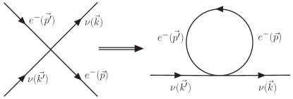
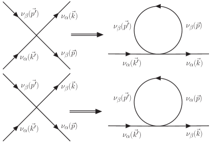
Figure 3: Mean-field approximation. Left: low energy diagrams for $\nu$-electron (top) and $\nu$-$\nu$ scattering (middle and bottom) that contribute to the neutrino evolution equations in dense media. Right: tadpole diagrams corresponding to the left ones in the mean-field approximation with ${\vec{p}}={\vec{p}}^{\prime}$. For the $\nu\nu$ interaction, the mean-field contributions have a diagonal (middle) and an off-diagonal (bottom) term (see text). (Figure from Volpe et al. [504]).

Besides the contributions from the neutrino mixings and the $\nu$-matter interactions, dense media have the peculiarity that neutral-current $\nu\nu$ interactions are sizable. In the mean-field approximation, the $\nu\nu$ Hamiltonian reads

$${\cal H_{\_}{\nu\nu,{\bf p}}}=\sqrt{2}G_{\_}{\rm F}\int_{\_}{p^{\prime}}(1-\hat{\bf p}\cdot\hat{\bf p}^{\prime})\left[\varrho_{\_}{{\bf p}^{\prime}}-\bar{\varrho}_{\_}{{\bf p}^{\prime}}\right]\,,$$ (15)

with

$$\int_{\_}{p^{\prime}}=\int d{\bf p}^{\prime}/(2\pi)^{3}\ ,$$ (16)

In the angular term on the r.h.s. of Eq.(15), $\hat{\bf p}={\bf p}/|{\bf p}|$ (similarly for $\hat{\bf p}^{\prime}$). The term $\hat{\bf p}\cdot\hat{\bf p}^{\prime}$ originates from the $V$-$A$ structure of the weak interactions and contributes in anisotropic dense media, playing a significant role.

More generally, the mean-field equations of motion that describe neutrino propagation in dense environments (and similarly antineutrinos) read

$$i(\partial_{\_}t+\mathbf{v}\cdot\mathbf{\nabla}_{\_}{\bf x}+\mathbf{F}\cdot\mathbf{\nabla}_{\_}{\bf p})\varrho_{\_}{\bf x,p}=[{\cal H}_{\_}{\bf x,p},\varrho_{\_}{\bf x,p}]\ ,$$ (17)

with $\mathbf{v}={\bf p}/E$ the neutrino velocity. In the Liouville operator on the l.h.s., the second term is an advective term which contributes in presence of spatial inhomogeneities. The third term depends on a possible external force $\mathbf{F}$, such as the gravitational one, that acting on the neutrinos can change its momentum or energy (because of trajectory bending for example). Since the Liouville operator depends on time, position and momentum, describing neutrino evolution in dense media is a 7-dimensional problem, and therefore extremely challenging numerically.

The solution of the neutrino mean-field equations reveals flavor mechanism that mostly arise from the interplay between the vacuum, the matter and the $\nu\nu$ contributions, as we now describe.

II.2 The MSW effect

The MSW effect is a reference phenomenon for flavor evolution studies. Several of the uncovered mechanisms are either MSW-like or multiple MSW phenomena. To clarify this link, we remind some basics.

The MSW effect arises when a resonance condition is satisfied, the resonance width is large and evolution through it is adiabatic. It is equivalent to the two-level problem in quantum mechanics [155].

Let us now introduce a new basis made of the eigenvectors for which the Hamiltonian describing neutrino propagation in an environment, is diagonal at each instant of time. This basis is called the matter basis and the corresponding eigenvalues the matter eigenvalues. In this section the neutrino Hamiltonian only comprises the vacuum and the matter contributions. More generally, a ”matter” basis can be introduced whatever terms are included in the Hamiltonian.

The flavor basis is related to the matter basis through the relation

$$|\nu_{\_}{\alpha}\rangle=\tilde{U}_{\_}{\alpha i}^{*}~{}|\tilde{\nu}_{\_}{i}\rangle\,,$$ (18)

with $i=1,2,3,...,N$ and $\alpha==e,\mu,\tau,\dots$. In the unitary matrix $\tilde{U}$, effective mixing parameters in matter replace the vacuum ones.

From Eqs. (5) and (18), one gets the following equation of motion for the matter basis

$$i{d\over dt}|\tilde{\nu}(t)\rangle={\cal\tilde{H}}~{}|\tilde{\nu}(t)\rangle=\Big{[}{\cal{\tilde{K}}}+i\tilde{U}^{\dagger}{d\tilde{U}\over{dt}}\Big{]} |\tilde{\nu}(t)\rangle\,,$$ (19)

where ${\cal{\tilde{K}}}={\rm diag}(\tilde{k}_{\_}1,\tilde{k}_{\_}2,\dots\tilde{k}_{\_}N)$ depends on the matter eigenvalues $\tilde{k}_{\_}i$ ($i=1,N$) and the matter Hamiltonian $\cal\tilde{H}$ now includes the derivatives of the effective mixing parameters in matter. These depend on the specific environment neutrinos are traversing.

Let us consider the explicit expressions for 2$\nu$ flavors for which equation (18) reads

$$\left(\begin{array}[]{c}|\nu_{\_}e\rangle\\ |\nu_{\_}x\rangle\end{array}\right)=\Big{(}\begin{tabular}[]{cc}1&0\\ 0&$e^{i\tilde{\beta}}$\\ \end{tabular}\Big{)}\Big{(}\begin{tabular}[]{cc}$\cos\tilde{\theta}$&$\sin\tilde{\theta}$\\ $-\sin\tilde{\theta}$&$\cos\tilde{\theta}$\\ \end{tabular}\Big{)}\left(\begin{array}[]{c}|\tilde{\nu}_{\_}1\rangle\\ |\tilde{\nu}_{\_}2\rangle\end{array}\right)\,,$$ (20)

with $\tilde{\theta}$ and $\tilde{\beta}$ the effective mixing angle and phase respectively. Neglecting the phase, the evolution equation of the matter basis (19) reads

$$i{d\over{dt}}\left(\begin{array}[]{c}|\tilde{\nu}_{\_}1\rangle\\ |\tilde{\nu}_{\_}2\rangle\end{array}\right)=\Big{(}\begin{tabular}[]{cc}$\tilde{k}_{\_}1$&$i\dot{\tilde{\theta}}$\\ -$i\dot{\tilde{\theta}}$&$\tilde{k}_{\_}2$\\ \end{tabular}\Big{)}\left(\begin{array}[]{c}|\tilde{\nu}_{\_}1\rangle\\ |\tilde{\nu}_{\_}2\rangle\end{array}\right)\,,$$ (21)

where the difference between $\tilde{k}_{\_}1$ and $\tilde{k}_{\_}2$ is given by

$$\tilde{k}_{\_}2-\tilde{k}_{\_}1=\sqrt{(\Delta m^{2}\cos 2\theta-A)^{2}+\Delta m^{2}\sin^{2}2\theta}\,.$$ (22)

In matter neutrinos acquire an effective mass. Figure 4 shows how $\tilde{k}_{\_}1$ and $\tilde{k}_{\_}2$ evolve as a function of the electron number density in an environment.

The effective mixing angle diagonalizing the $2\times 2$ matrix given by equation (11) satisfies

$$\sin^{2}2\tilde{\theta}={{\Delta m^{2}\sin^{2}2\theta}\over{(\Delta m^{2}\cos^{2}2\theta-A)^{2}+\Delta m^{2}\sin^{2}2\theta}}\,,$$ (23)

with $A=2EH_{\_}{\rm CC}^{\nu e}$ Eq.(7).

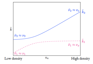
Figure 4: The Mikheev-Smirnov-Wolfenstein effect: matter eigenvalues of the heavier (solid) and lighter (dashed) matter eigenstates, as a function of the electron number density $n_{\_}e$. The matter eigenvalues $\tilde{k}_{\_}2$ and $\tilde{k}_{\_}1$ evolve from the inner dense regions of a star (right) to the star surface (left part of the figure), where $\tilde{\nu}_{\_}2,\tilde{\nu}_{\_}1$ become the neutrino mass eigenstates in vacuum $\nu_{\_}2$ and $\nu_{\_}1$ respectively. The MSW resonance is at the location where the matter eigenvalues are the closest and the matter mixing angle maximal. The MSW effect is a two-level problem in quantum mechanics. (Figure from [142]).

One can see that, when the following equality holds

$$\sqrt{2}G_{\_}{\rm F}n_{\_}e={\Delta m^{2}\over{2E}}\cos 2\theta\,,$$ (24)

the matter mixing angle is maximal, i.e. $\tilde{\theta}=\pi/4$, and the distance between the matter eigenvalues minimal (Fig. 4).

Relation (24) corresponds to the difference of the diagonal elements in the Hamiltonian Eq.(11) being equal to zero (or to a minimal distance of the matter eigenvalues in the matter basis). It is the MSW resonance condition. In the usually adopted convention, the fulfillment of relation (24) implies that, since $\theta<\pi/4$ and $\cos 2\theta>0$, $\Delta m^{2}>0$ to have the r.h.s. positive. Therefore the occurrence of the MSW effect gives the sign of the mass-squared difference.

When the resonance condition is satisfied, and its width

$$\Gamma_{\_}{\rm MSW}=\Delta m^{2}\sin^{2}2\theta\,,$$ (25)

large, the fate of neutrinos depends on the adiabaticity of the neutrino evolution through the resonance. As in the two-level problem in quantum mechanics, adiabaticity through the resonance can be quantified by the adiabaticity condition (see e.g. [249])

$$\gamma^{-1}={2|\dot{\tilde{\theta}}|\over {\tilde{k}_{\_}2-\tilde{k}_{\_}1}}={{\Delta m^{2}}\over{2E}}{{\sin^{2}2\theta}\over{\cos 2\theta}}{{n_{\_}e}\over{|dn_{\_}e/dr|}}\ll 1\,,$$ (26)

where $\gamma$ is the adiabaticity parameter. Eq.(26) corresponds to adiabatic evolution; whereas if $\gamma^{-1}\gg 1$, evolution is fully non-adiabatic. Indeed, it is the derivative of the matter mixing angle that governs the mixing between the matter eigenstates Eq.(21), but how significant is its impact on the neutrino evolution depends on the ratio of the off-diagonal terms of the Hamiltonian over the difference of the diagonal terms. If the former are much smaller than the latter, the adiabaticity condition Eq.(26) holds and each mass eigenstate only acquires a phase during the evolution from the inner regions to the surface of the star.

Let us consider again the case of solar neutrinos. In the dense inner regions of the Sun, the matter mixing angle $\tilde{\theta}$ is close to $\pi/2$: the matter and flavor eigenstates practically coincide. If a neutrino, initially produced as a $\nu_{\_}e$ coincides with $\tilde{\nu}_{\_}2$ evolves through the MSW resonance adiabatically it emerges as a $\nu_{\_}2$ at the surface of the star (Fig. 4). A significant fraction of the $\nu_{\_}e$ flux is then detected as $\nu_{\_}{x}$ on Earth. Note that, if the vacuum mixing angle had been small (as believed historically), the MSW effect would have produced a spectacular matter enhanced conversion of $\nu_{\_}e$ into the other flavors.

The survival probability of solar $\nu_{\_}e$, averaged over the production region, reads [398]

$$\langle P(\nu_{\_}e\rightarrow\nu_{\_}e)\rangle={1\over 2}+({1\over 2}-P_{\_}{h})\cos 2\tilde{\theta}^{(i)}\cos 2\theta\ ,$$ (27)

where $\tilde{\theta}^{(i)}$ is the mixing angle at production at high density. The quantity $P_{\_}{h}$ is the probability of $\tilde{\nu}_{\_}2$ to $\tilde{\nu}_{\_}1$ transitions, and is thus related to the mixings of the matter eigenstates at the MSW resonance. In the adiabatic case, the mixing is suppressed, $P_{\_}h=0$. For the large mixing angle $\theta=35^{\circ}$, equation (27) gives $\langle P(\nu_{\_}e\rightarrow\nu_{\_}e)\rangle=\sin^{2}\theta=0.33$, as observed for solar ⁸B neutrinos.

The observation of solar neutrinos by the SNO experiment, through charged-current and neutral-current interactions of neutrinos on deuterium and neutrino-electron elastic scattering, allowed to measure the total solar neutrino flux and showed unambiguous conversion of $\nu_{\_}e$ to the other active $\nu_{\_}{\mu}$ and $\nu_{\_}{\tau}$ flavors [34]. Moreover KamLAND measurement of reactor $\bar{\nu}_{\_}e$ disappearance showed oscillations with $\Delta m^{2}=6.9\times 10^{-5}$ eV² and $\sin 2\theta=1.0$ (best fit) thus identifying the MSW solution to the solar neutrino problem, with the large mixing angle [197].

So, the MSW effect is responsible for a reduction of the ⁸B solar neutrino flux to 1/3 the value predicted by the Standard Solar Model. Since the MSW resonance condition is satisfied for the high energy solar neutrinos, this gives us the sign of the corresponding mass-squared difference: $\Delta m_{\_}{12}^{2}>0$.

Let us now come back to the concept of adiabaticity more generally. The adiabaticity condition, defined as the ratio of (twice) the modulus of the off-diagonal term of the neutrino Hamiltonian over the difference of the diagonal ones, can be generalized in presence, for example, of $\nu\nu$ interactions as done in Galais et al. [236]. In this case the condition also involves the derivatives of the phase that arise because of the complex contribution, to the neutrino Hamiltonian, due to the neutrino-neutrino interaction Eq.(15).

When the matter density changes smoothly, neutrinos evolve through the resonance ”adjusting” to the density variation: evolution is adiabatic. This contrasts with what happens when steep variations of the density profiles are present, as e.g. in presence of shock waves.

With the spin formalism, we look at flavor phenomena with different eyes, since we follow neutrinos through the evolution of effective spin ${\rm{\bf P}}$, subject to effective magnetic fields (see Appendix A and [155]). In this context, vacuum oscillation is a precession of neutrino spins in flavor space, around the vacuum (effective) magnetic field ${\rm{\bf B}}_{\_}{\rm vac}$ tilted by $2\theta$ [304, 303] (Fig. 5). One can show that, from the evolution of the third component $P_{\_}z$, one recovers the vacuum oscillation formula.

As for the MSW effect, it takes place in matter when ${\rm{\bf P}}$ goes through the $x$-$y$ plane, since the MSW resonance condition Eq.(24) corresponds to $P_{\_}z=0$. Adiabatic evolution occurs when the precession frequency of ${\rm{\bf P}}$ around ${\rm{\bf B}}={\rm{\bf B}}_{\_}{\rm vac}+{\rm{\bf B}}_{\_}{\rm mat}$ is fast compared to the rate with which ${\rm{\bf B}}$ changes, so that neutrino spins follow the magnetic field during propagation. On the contrary, if evolution is non-adiabatic, ${\rm{\bf P}}$ ”lags behind”.

The theoretical description in terms of neutrino isospins has been largely exploited to study neutrino flavor evolution in dense environments and in particular when $\nu\nu$ interactions are sizable (see for example the review by Duan et al. [191]).

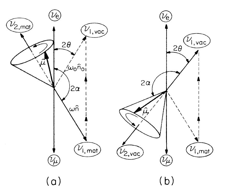
Figure 5: Spin formalism: picture of the neutrino evolution in flavor space for $2\nu$ flavors. The third component of the neutrino spin vector corresponds either to $\nu_{\_}e$ (upward) or to $\nu_{\_}{\mu}$ (downward). When electron neutrinos are produced in the Sun, the vector ${\bf\mu}$ (${\bf P}$ in the text) precess around the matter vector ${\bf n}$ (${\bf B_{\_}{\rm mat}}$ in the text) and, if evolution is adiabatic, it follows ${\bf n}$ until it becomes the vacuum vector ${\bf n}_{\_}0$ (${\bf B_{\_}{\rm vac}}$ in the text). The latter is tilted by $2\theta$ with respect to the $z$-axis. (Figure from Kim et al. [303].)

II.3 The MSW effect in dense media

Neutrinos face more than one resonance if the density is large as e.g. in astrophysical environments or the early universe. Although we will mostly refer here to supernova neutrinos as an example, the aspects we cover can be transposed to other dense environments, such as binary neutron star mergers. In our discussion, we will assume that, unless differently stated, the $\nu_{\_}{\mu},\nu_{\_}{\tau}$ and $\bar{\nu}_{\_}{\mu},\bar{\nu}_{\_}{\tau}$ fluxes (referred to as $\nu_{\_}x$ and $\bar{\nu}_{\_}x$ respectively) are equal, as in nearly all the available literature.

Dighe and Smirnov [184] pointed out that there are three MSW resonances in supernovae: the high (H-), the low (L-) and the $V_{\_}{\mu\tau}$. As the MSW resonance condition shows, the resonance location depends on the neutrino energy and mixing parameters. From Eq. (24) one finds that the H- and L-resonances, associated with $(\theta_{\_}{31},\Delta m^{2}_{\_}{31})$ and $(\theta_{\_}{21},\Delta m^{2}_{\_}{21})$ respectively, take place at

$$\rho_{\_}{\rm res}\simeq 1.4\times 10^{6}~{}{\rm g\over{cm^{3}}}\Big{(}{{\rm\Delta m^{2}}\over 1~{}{\rm eV}^{2}}\Big{)}\Big{(}{15~{}{\rm MeV}\over E}\Big{)}\Big{(}{0.5\over Y_{\_}e}\Big{)}\cos 2\theta\,.$$ (28)

where the electron fraction $Y_{\_}e$ is given by

$$Y_{\_}e={{n_{\_}e-n_{\_}{\bar{e}}}\over{n_{\_}B}}\ ,$$ (29)

that is, it is the net number of electrons (the difference between the electron and positron number densities) per baryon $n_{\_}B=n_{\_}p+n_{\_}n$ ($n_{\_}p$ is the proton number density). Therefore, for a 40 MeV neutrino, one finds $\rho_{\_}{res}=1.2\times 10^{3}$ g/cm³ for the H–resonance and $\rho_{\_}{res}=13$ g/cm³ for the L-resonance ($Y_{\_}e=0.5$).

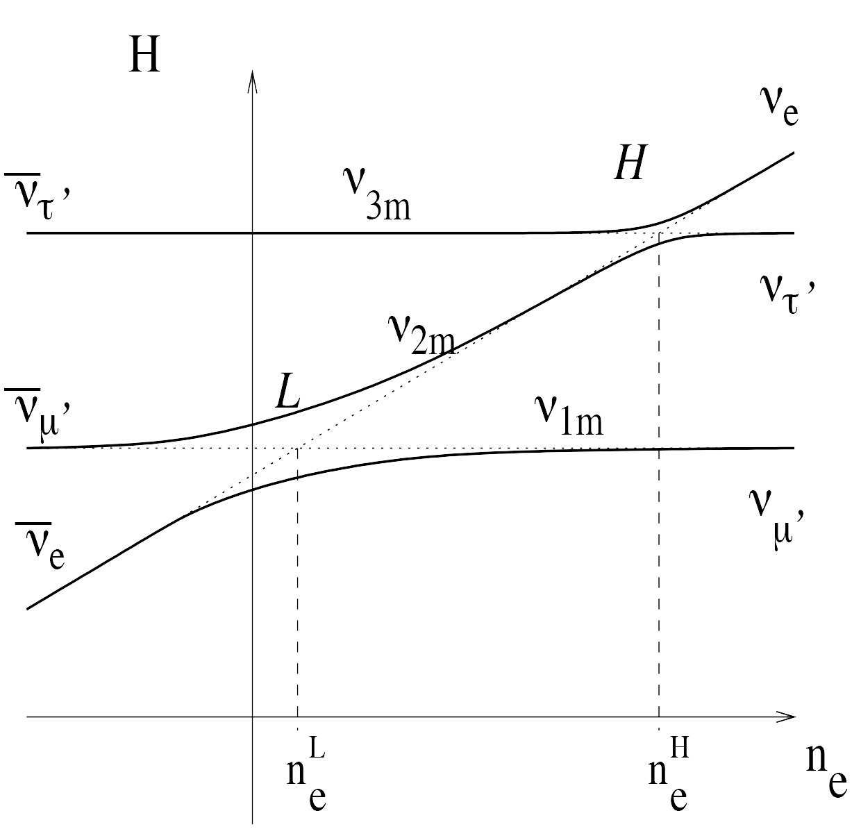
Figure 6: MSW effect in core-collapse supernovae: effective neutrino masses as a function of the electron number density in absence (dashed) or in presence (solid lines) of neutrino mixings. The high (H-) and low (L-) MSW resonances are indicated, whereas the $V_{\_}{\mu\tau}$ resonance (at higher density) is not shown. Note that the antineutrino case is represented in the part of the plot with negative electron number density. The diagram corresponds to normal mass ordering. (Figure adapted from [184].)

Moreover radiative corrections that differentiate $\nu_{\_}{\mu}$ and $\nu_{\_}{\tau}$ [114], introduce the potential $V_{\_}{\mu\tau}=10^{-5}V_{\_}{\rm CC}$ where $V_{\_}{\rm CC}$ is given by Eq.(7). The quantity $V_{\_}{\mu\tau}$ becomes relevant if the medium is very dense (i.e. for densities larger than $10^{7}$-$10^{8}$ g/cm³). The $V_{\_}{\mu\tau}$ resonance is associated with the atmospheric mixing parameters $(\theta_{\_}{32},\Delta m^{2}_{\_}{32})$. Figure 6 shows the eigenvalues of the neutrino Hamiltonian given by Eq.(9) and including the $V_{\_}{\mu\tau}$ potential, in the ($\nu_{\_}e,\nu_{\_}{\mu}^{\prime},\nu_{\_}{\tau}^{\prime}$) basis which is a rotated ($\nu_{\_}e,\nu_{\_}{\mu},\nu_{\_}{\tau}$) basis where the ($\nu_{\_}{\mu},\nu_{\_}{\tau}$) sub-matrix of the neutrino Hamiltonian is diagonal.

As is well known, the supernova neutrino time signal comprises three characteristic phases of the supernova dynamics and explosion called the neutronization burst, the accretion phase and the cooling phase of the newly-born proto-neutron star (see Fig.23, section IV.B and for example the reviews by Mirizzi et al. [367] and Vitagliano et al. [495]). The neutrino spectra depend on these phases, on the supernova progenitor and on the direction of observation, in particular because of the SASI and LESA instabilities. For what follows, the explicit time dependence of the neutrino signals is not necessary.

A characteristic feature of flavor phenomena is that they induce spectral modifications. Let us consider the neutrino spectra at the neutrinosphere, $\phi^{0}_{\_}{\bar{\nu}_{\_}e}$ and $\phi^{0}_{\_}{\bar{\nu}_{\_}x}$ (thought as a function of time, or as fluences, i.e. time-integrated fluxes) and assume $\nu$ evolution through H- and L-resonances only in terms of probabilities. For example, if $\bar{\nu}_{\_}e$, produced in the inner stellar regions, traverse the three resonances, their spectra become

$$\phi_{\_}{\bar{\nu}_{\_}e}=\bar{p}\phi^{0}_{\_}{\bar{\nu}_{\_}e}+(1-\bar{p})\phi^{0}_{\_}{\bar{\nu}_{\_}x}\,,$$ (30)

where $\bar{p}$ is the spectral swapping probability. In particular, $\bar{p}=0.68$ and $\bar{p}=0$ for normal and inverted mass ordering respectively.

As supernova simulations show, the neutrino spectra at the neutrinospheres, $\phi^{0}_{\_}{\bar{\nu}_{\_}e}$ and $\phi^{0}_{\_}{\bar{\nu}_{\_}x}$, are well described by pinched Fermi-Dirac distributions [184] or by power laws [301]. Because of their microscopic interactions, the neutrino average energies often satisfy the (approximate) hierarchy $\langle E_{\_}{\nu_{\_}e}\rangle<\langle E_{\_}{\bar{\nu}_{\_}e}\rangle<\langle E_{\_}{\nu_{\_}x}\rangle$, with typical energies $E_{\_}{\nu_{\_}e}\in[8,14]$ MeV, $E_{\_}{\bar{\nu}_{\_}e}\in[14,18]$ MeV and $E_{\_}{\nu_{\_}x}\in[16,20]$ MeV. In fact, $\nu_{\_}x$ undergo neutral current interactions and decouple from deeper hotter regions. Unlike $\nu_{\_}x$, $\nu_{\_}e$ and $\bar{\nu}_{\_}e$ interact via charged- and neutral-current interactions and decouple from colder outer shells.

From Eq.(30), one sees that, in case of inverted mass ordering, due to the MSW effect, $\bar{\nu}_{\_}e$ can acquire the hotter spectra of the non-electron flavor neutrinos (if the latter have a higher average energy at the neutrinosphere). A similar mechanism occurs to the $\nu_{\_}e$ spectra, if the mass ordering is normal. If a supernova blows off, such spectral modifications will impact charged-current events associated with inverse-$\beta$ decay or neutrino-nucleus interactions, in a scintillator, Cherenkov, lead, or liquid argon supernova neutrino detector. On the contrary, neutral-current events are ”flavor blind” and therefore not sensitive to spectral swapping.

It is important to keep in mind that if, under some conditions, the supernova fluxes of the different neutrino flavors become (practically) degenerate, then spectral distortions due to flavor mechanisms, according e.g. to (30), impact neither directly nor indirectly observations. For this reason, the possibility of flavor equilibration is often discussed in the literature and theorists have been actively looking for this simplifying possibility.

A few more remarks. First, in core-collapse supernovae, for typical matter profiles (in absence of shock waves), the evolution through the L-resonance is adiabatic. Second, as mostly assumed in the literature, if $\phi^{0}_{\_}{\bar{\nu}_{\_}{\tau}}=\phi^{0}_{\_}{\bar{\nu}_{\_}{\mu}}$ at tree level, the $V_{\_}{\mu\tau}$ resonance, which mixes $\nu_{\_}{\mu}$ and $\nu_{\_}{\tau}$, does not produce spectral modifications and therefore observables effects. Note however that, if one includes muons and six-species neutrino transport in supernova simulations [110], $\nu_{\_}{\mu}$ and $\nu_{\_}{\tau}$ fluxes can differ at tree level. The study of the impact of the six-species neutrino transport on neutrino flavor evolution is ongoing. Third, the only unknown parameter that impacts the standard MSW effect is the neutrino mass ordering, since the sign of $\Delta m^{2}_{\_}{23}\approx\Delta m^{2}_{\_}{13}$ is not determined yet. Therefore, the detection of the neutrino signal from a future galactic supernova could inform us on this key property, as we shall see.

Let us now discuss multiple MSW resonances and MSW-like mechanisms that arise in dense astrophysical environments such as an exploding supernova.

II.4 Shock wave effects

Shock-related structures in supernova neutrino observations could inform us on shock reheating and propagation, a unique observation of the explosion mechanism on its becoming. The availability of large scale observatories and a close supernova would offer the possibility to observe such structures and other deviations from the expected exponential cooling of the newly formed neutron star. Even if there are variations among models, some features appear as sufficiently generic to deserve investigation.

In an exploding supernova, shock waves constitute a major perturbation of the electron fraction $Y_{\_}e$, and of the pre-supernova matter density profiles. The shock wave reaches the H-resonance region in about 2 s after core-bounce. Tomàs et al. [485] showed the presence of both a front and a reverse shock, due to the earlier slower ejecta meeting a hot supersonically expanding neutrino-driven wind (Fig. 7).

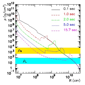
Figure 7: Shock waves: matter density profiles, at different post-bounce times, as a function of distance in an exploding core-collapse supernova model. Front and reverse shocks are visible. The yellow and blue bands correspond to the densities and neutrino energies that fulfill the high (H-) and low (L-) MSW resonance conditions. (Figure from [485].)

Schirato and Fuller [451] first pointed out that shock waves could ”shut off” flavor evolution when passing through an MSW resonance region. Because of the steepness of the density profile, $\nu_{\_}{\mu,\tau}\leftrightharpoons\nu_{\_}{\rm e}$ would be suppressed due to non-adiabatic evolution. Hence the $\nu_{\_}{\rm e},\bar{\nu}_{\_}e$ fluxes would become colder producing dips in the supernova neutrino time signal.

The passage of shock waves in MSW resonance regions engenders two effects: it makes the resonance temporarily non-adiabatic and induces multiple MSW-resonances. The evolution through the different resonance locations can be treated as incoherent or as coherent. In the former, the MSW resonances are independent, in the latter coherent evolution produces interference effects among the matter eigenstates called phase effects. Since the MSW resonance condition is necessary for shock wave effects, they occur either in the $\nu_{\_}e$ signal (for normal), or in the $\bar{\nu}_{\_}e$ signal (for inverted mass ordering).

The change in the adiabaticity at the MSW resonance locations impacts the evolution in the H-resonance region and modifies the neutrino average energies creating dips or bumps in the supernova time signal and the corresponding rates. These features were investigated in a series of works [476, 218, 336, 222, 307], see the review by Duan and Kneller [192]).

Fogli et al. [218] pointed out that multiple resonances could produce phase effects that would average out for large values of $\theta_{\_}{13}$. Dasgupta and Dighe [165] investigated them in detail. Phase effects require semi-adiabatic and coherent evolution at the resonances. They are difficult to be seen because even when the coherence condition is met, the associated oscillations are smeared by the energy resolution of detectors.

Let us consider the presence of a dip in a supernova density profile as an example. A neutrino of energy $E$ encounters two resonances at locations $x_{\_}1$ and $x_{\_}2$. If $|\nu_{\_}h\rangle$ and $|\nu_{\_}l\rangle$ are the heavier and lighter matter eigenstates respectively, at $x<x_{\_}1$, one has $|\nu_{\_}h\rangle(x\ll x_{\_}1)\approx|\nu_{\_}e\rangle$. While evolution before the resonance is adiabatic, the resonance mixes the matter eigenstates just before the crossing $x<x_{\_}{1-}$ yielding new matter eigenstates

$$\left(\begin{array}[]{c}|\nu_{\_}h(x_{\_}{1+})\rangle\\ |\nu_{\_}l(x_{\_}{1+})\rangle\end{array}\right)=\Big{(}\begin{tabular}[]{cc}$\cos\chi_{\_}1$&$\sin\chi_{\_}1e^{i\phi}$\\ $-\sin\chi_{\_}1e^{-i\phi}$&$\cos\chi_{\_}1$\\ \end{tabular}\Big{)}\left(\begin{array}[]{c}|\nu_{\_}h(x_{\_}{1-})\rangle\\ |\nu_{\_}l(x_{\_}{1-})\rangle\end{array}\right)\,,$$ (31)

where $P_{\_}i=\sin^{2}\chi_{\_}1$ is the hopping probability for an isolated resonance. The matter eigenstates acquire a relative phase up to the second resonance at $x_{\_}2$. After the latter the $\nu_{\_}e$ survival probability is (far from $x_{\_}2$)

$$P({\nu_{\_}e\rightarrow\nu_{\_}e}) =\cos^{2}(\chi_{\_}1-\chi_{\_}2)$$ (32)

$$-\sin 2\chi_{\_}1\sin 2\chi_{\_}2\sin^{2}\Big{(}\int_{\_}{x_{\_}1}^{x_{\_}2}{{\Delta\tilde{m}^{2}}\over{4E}}dx\Big{)}\,.$$

The last term, due to the interference between the matter eigenstates, oscillates with the neutrino energy and with the resonance locations. It produces fast oscillations (the phase effects) as a function of energy or, for a given energy, as a function of distance (or time) because the shock wave propagation slightly shifts such locations. In absence of coherence, the interference term averages out and the two resonances at $x_{\_}1$ and at $x_{\_}2$ are independent.

Two studies implemented shock wave effects and $\nu\nu$ interactions (in the bulb model). Using a consistent treatment that retains phase information, Gava et al. [244] showed that, depending on the neutrino energy, dips or bumps are present in the positron time signal, due to inverse-beta decay (i.e. $\bar{\nu}_{\_}e+p\rightarrow e^{+}+n$), of scintillators or Cherenkov detectors (inverted mass ordering). Similar features are present, for normal mass ordering, in the electron time signal of an argon-based detectors e.g. DUNE, due to charged-current $\nu$-⁴⁰Ar interactions. In contrast, the detailed analysis of the time signal for the lead detector HALO-2 performed by Ekinci et al. [201] showed changes at the level of a few percent for the one-neutron and two-neutron emission rates in neutrino-lead interactions, so too small to be seen.

Besides shock waves, turbulence can play a significant role in supernova explosions (see for example Radice et al. [419]). The influence of turbulence on the neutrino flavor content has features in common with shock wave effects, as we shall now discuss.

II.5 Turbulence effects

Noisy media, originating e.g. from helioseismic g-modes or temperature fluctuations, influence neutrino flavor evolution, as pointed out in relation with the solar neutrino problem (see for example Sawyer [446], Nunokawa et al. [385], Balantekin et al. [70]). In particular, Loreti and Balantekin [328] showed that randomly fluctuating matter density and magnetic fields tend to depolarize neutrinos, i.e. the survival probability averages to one-half. Neutrino propagation in stochastic media was also discussed in Torrente-Lujan [486], Burgess and Michaud [120].

Interestingly, solar neutrino and KamLAND data constrain matter density fluctuations in our Sun at a few percent level. This result holds for delta correlated (white) noise, and correlation lengths of 10 km to 100 km (see Balantekin and Yüksel [76], Guzzo et al. [262]). Hence, one can extract the solar oscillation parameters independently from fluctuations [119].

Simulations of exploding core-collapse supernovae show that non-radial turbulent flows associated with convection and SASI have explosion supportive effects [362, 290, 159, 291, 419, 224]. Hydrodynamic instabilities generate large scale anisotropies between the proto-neutron star and the supernova envelope. Therefore, supernova neutrinos reaching the Earth ”see” stochastic matter density profiles.

Noisy media might influence the supernova neutrino flavor content significantly. First investigations evolved fluctuations-averaged density matrices, or probabilities, with delta-correlated fluctuations and static [329] or dynamic density profiles with front and reverse shocks [223]. Friedland and Gruzinov [228] argued for Kolmogorov correlated fluctuations.

Kneller and Volpe [308] evolved neutrino amplitudes and built a statistical ensemble of instantiations for the neutrino survival probabilities using one-dimensional simulations and Kolmogorov fluctuations added. Retaining the phase information, the approach revealed the presence of multiple MSW resonances from turbulence and a transition, when increasing the fluctuations amplitude, from phase effects due to shock waves to a fluctuations dominated regime. Lund and Kneller [339] investigated the interplay between neutrino-neutrino interactions, shock waves and turbulence using one-dimensional dynamical simulations for three progenitors. These studies showed that large amplitude fluctuations resulted into depolarization of the neutrino probabilities [329, 223, 228, 308].

Borriello et al. [113] came to different conclusions. The authors performed the first investigation exploiting fluctuations from high resolution two-dimensional supernova simulations down to scales smaller than typical matter oscillation lengths. These fluctuations followed broken power laws (with exponents 5/3 and 3) in agreement with two-dimensional Kolgomorov-Kraichnan theory of turbulence. Their analysis showed small damping of the neutrino probabilities due to matter fluctuations and absence of strong or full depolarization.

Clearly further work is needed to determine the impact of turbulence on flavor evolution and to assess if matter fluctuations introduce a loss of memory effects, or not.

II.6 MSW-like mechanisms

The MSW effect arises from the cancellation of the vacuum and the matter contributions. New resonance conditions emerge from the interplay of the different terms of the neutrino Hamiltonian Eq.(6) describing neutrino propagation in a dense medium. Thus, various types of MSW-like phenomena have been uncovered, in particular the matter-neutrino resonance, helicity coherence and the I-resonance that we shall now describe.

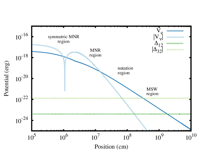
Figure 8: Matter-neutrino resonances: potentials of the neutrino Hamiltonian, as a function of distance, in an accretion disk model of a black hole-neutron star merger. Regions are indicated where different neutrino flavor mechanisms take place. The $\nu\nu$ interaction and the matter terms ($V_{\_}e=H_{\_}{\rm CC}^{\nu e}$) cross at the locations of the symmetric and standard MNRs. Note that $|V_{\_}{\nu}|$ indicates the only non-zero term of the $\nu\nu$ Hamiltonian, in a disk geometry, at initial time. The nutation region is a region where oscillations occur due to a cancellation between the $\nu\nu$ interactions and the vacuum ($\Delta_{\_}{32}$) terms. The MSW region is also shown. Note that $\Delta_{\_}{12}=\Delta m^{2}_{\_}{12}$ and $|\Delta_{\_}{32}|=|\Delta m^{2}_{\_}{32}|$. (Figure adapted from [346].)

II.6.1 Matter-neutrino resonance

Accretion disks around compact objects – binary neutron star merger remnants or black holes – produce large amounts of neutrinos with luminosities and average energies similar to those of core-collapse supernovae. An important difference is that, in these environments, matter is neutron-rich which produces an excess of the $\bar{\nu}_{\_}e$ flux over the $\nu_{\_}e$ one. Computationally, even the simplest models require spherical symmetry breaking which is numerically more involved. It is to be noted that, in the context of core-collapse supernovae, spherical symmetry was assumed in numerous studies which yielded interesting results.

In a collapsar-type disk, Malkus et al. [345] found a novel conversion mechanism called the matter-neutrino resonance (MNR). The MNR arises in regions above the disk when the $\nu$-matter and the $\nu\nu$ interactions cancel each other (Figs. 8 and 9). Indeed, the excess of the $\bar{\nu}_{\_}e$ flux over the $\nu_{\_}e$ one gives a different sign to the two contributions giving the possibility of a cancellation. Moreover, because of the geometry of the disks and the $\bar{\nu}_{\_}e$s decoupling deeper than $\nu_{\_}e$s, the sign of the only non-zero element of the $\nu\nu$ Hamiltonian at initial time (i.e. the $ee^{th}$) can flip at some location. If the flip in sign is not present the phenomenon is called standard MNR [344]; whereas if it is present, the process is called the symmetric MNR [345, 346] (Fig. 8). Adiabatic evolution through the MNRs produces efficient conversion of ${\nu}_{\_}e$ into ${\nu}_{\_}{\mu},{\nu}_{\_}{\tau}$ for the former; or of $\nu_{\_}e$ and $\bar{\nu}_{\_}e$ for the latter. This can influence the electron fraction $Y_{\_}e$ and favor disk wind nucleosynthesis of $r$-process elements (Fig. 10).

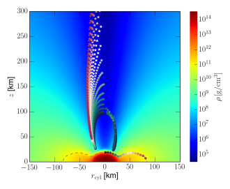
Figure 9: Matter-neutrino resonances: the central object at the bottom is a binary neutron star merger remnant, with its accretion disk (dashed line). The stars indicate the locations where the MNR resonance condition is fulfilled along different trajectories above the remnant. (Figure from [227].)

Zhu et al. [531] and Frensel et al. [227] showed that patterns of flavor evolution depend on the neutrino path. Both studies were based on astrophysical inputs from the detailed two-dimensional simulations of a binary neutron star merger remnant by Perego et al. [408]. Considering different initial conditions and azimuthal angles, Frensel et al. [227] also found that the neutrino capture rates on neutrons and protons showed variations by tens of percent due to flavor mechanisms.

In these studies the $\nu\nu$ Hamiltonian Eq.(15) is treated by taking the flavor history of one neutrino as representative of all trajectories. A consistent treatment of the neutrino-neutrino interaction term should also implement the neutrino evolution along different paths. Vlasenko and McLaughlin [498] showed that, even when a more consistent treatment is used, the MNRs take place leading to significant neutrino conversion.

What is the underlying mechanism of the matter-neutrino resonances? Wu et al. [512], with a schematic model, and Chatelain and Volpe [143], with detailed BNS simulations, showed the MNRs are multiple MSW resonances. The crossing of the potentials shows the location where the MNR starts (Fig. 8). Furthermore if one looks at the full evolution of the Hamiltonian, the matter and the $\nu\nu$ interaction terms cancel for tens of km, concomitantly with the MNR process. Indeed, using a perturbative argument, Chatelain and Volpe [143] showed that the $\nu\nu$ interactions adjust to the matter term over long distances: the MNR condition is fulfilled multiple times due to the non-linearity of the equations and non-linear feedback.

II.6.2 Spin or helicity coherence

The derivation of extended mean-field equations beyond the ones usually employed in flavor studies uncovered new terms (see Section II.A). Thanks to these, new resonances become possible that can influence the neutrino content.

Already long ago, Rudzsky [437] had pointed out wrong helicity contributions. Volpe et al. [504] derived mean-field equations including pairing correlators and wrong-helicity contributions, due to the neutrino mass. Afterwards Vlasenko et al. [496] obtained quantum kinetic equations for Majorana neutrinos, using the Closed-Time-Path formalism, and pointed to wrong-helicity terms $\sim m/E$ naming them spin coherence. Serreau and Volpe [457] presented the most general mean-field equations and called such contributions helicity coherence. Present in anisotropic media, they couple neutrinos with antineutrinos but are suppressed, as expected, by the ratio $m/E$.

In a toy 2$\nu$ model Vlasenko et al. [497] first studied if helicity coherence modifies flavor. The authors found that it could trigger significant $\nu$-$\bar{\nu}$ transformation through non-linear feedback. Motivated by such findings, Chatelain and Volpe [143] investigated these terms in binary neutron star mergers with inputs from detailed simulations. In contrast with the previous findings, their results showed that, while the resonance condition for helicity coherence (similar to the MNR one) was fulfilled, adiabatic evolution was absent for the ensemble of trajectories considered. Indeed, the authors were able to show that non-linear feedback could not induce multiple matching of the resonance conditions, contrarily to the MNR. The subsequent work of Tian et al. [484] on the role of helicity coherence in core-collapse supernovae reached similar conclusion.

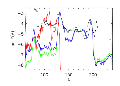
Figure 10: Nucleosynthetic abundances: the crosses show the scaled solar abundances. Visible are the second peak (around A=130-138) and the third peak (around A=195-208) as well as the rare elements plateau in-between. The observations are compared with predictions of nucleosynthetic abundances in a black hole-accretion disk scenario. The lines correspond to results in absence of neutrino oscillations (red), with oscillations (blue) or without the $\nu\nu$ interaction (green). The results are for normal neutrino mass ordering. (Figure from [345].)

II.6.3 I-resonance

Non-standard interactions are present in theories beyond the Standard Model. Limits on non-standard neutrino-neutrino interactions are rather loose [103]; whereas oscillations and scattering experiments provide tight constraints on non-standard neutrino-matter interactions (NSI) (see for example the reviews by Ohlsson [389], Davidson et al. [172], Farzan and Tortola [209], Biggio et al. [102]). After decades of attempts, Akimov et al. [39] (COHERENT Collaboration) measured coherent neutrino-nucleus scattering, giving, among others, new constraints [158, 248].

NSI are often evoked in the interpretation of neutrino oscillation experiments, as possible explanations of anomalies. If NSI exist, mixing angles and mass-squared differences inferred by experiments are modified. In dense astrophysical environments, NSI were studied by several authors [220, 206, 207, 464, 144]. Their results highlighted that NSI significantly impact flavor evolution. Moreover the role of non-standard neutrino-neutrino interactions in supernovae was also studied by Blennow et al. [107]. In the context of primordial nucleosynthesis, NSI give a subleading contribution to the effective number of degrees of freedom [348].

Esteban-Pretel et al. [206, 207] explored the combined effect of $\nu\nu$ interactions and $\nu$-matter NSI in core-collapse supernovae. For NSI couplings $|\epsilon|\geq 10^{-2}$, an MSW-like phenomenon called the I-resonance emerges. It takes place for $\nu$ and $\bar{\nu}$ simultaneously when the standard and non-standard matter terms cancel each other. The I-resonance triggers efficient conversions of $\nu_{\_}{\rm e}\rightarrow\nu_{\_}{\mu,\tau}$ and $\bar{\nu}_{\_}{\rm e}\rightarrow\bar{\nu}_{\_}{\mu,\tau}$ independently from the neutrino energy.

Stapleford et al. [464] performed an extensive investigation of NSI effects as a function of their couplings. The authors found that, even for NSI strengths well below bounds, NSIs produce (symmetric and standard) MNRs in core-collapse supernovae and impact the MSW-H resonance and $\nu\nu$ interactions effects (bulb model, see section II.G.1).

The first investigation of NSI effects in BNS was performed by Chatelain and Volpe [144]. They showed that neutrino-neutrino interactions play a role on the I-resonance, contrarily to previous findings. Indeed, when the $\nu\nu$ interactions matter, the I-resonance becomes a synchronized MSW effect. The investigation of a large ensemble of trajectories, above a BNS remnant, uncovered that, as in core-collapse supernovae, even very small values of NSI parameters produce intricate patterns of mechanisms, including MNRs (Fig. 11), I- and synchronized I-resonances.

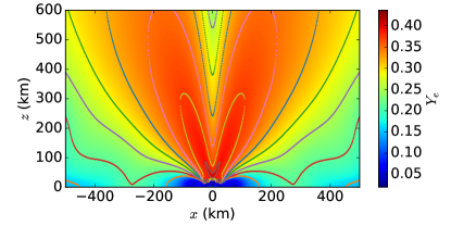
Figure 11: I-resonances: the lines indicate the locations where the I-resonance condition is fulfilled above a binary neutron star merger remnant (at the centre, bottom of the figure). Values of the electron fraction $Y_{\_}e$, in absence of flavor evolution, are coded with colors. (Figure from [144].)

II.7 Neutrino-neutrino interactions

Dense environments have sizable $\nu\nu$ standard neutral-current interactions because neutrinos are emitted in large amounts. In a seminal work, Pantaleone [397] pointed out that the $\nu\nu$ interactions introduce off-diagonal potentials and make $\nu$ evolution a non-linear many-body problem.

In the last fifteen years theorists have tirelessly worked to understand the neutrino-neutrino refraction effects, the novel flavor mechanisms, how they arise and their impact. They have established connections with other many-body systems and figured out new approaches to deal with such interactions. Several reviews dress a detailed picture of these developments [191, 192, 367, 502, 284, 482]. Here I shall highlight aspects emerged from the efforts to solve this complex problem.

Flavor mechanisms due to $\nu\nu$ interactions are currently classified as slow or as fast. Slow modes occur at typical distances of $\mathcal{O}(10^{2}$-$10^{3})$ km from the neutrinosphere, whereas fast modes have scales of $\mathcal{O}(1)$ m or much less and frequencies as large as $\mu\sim\sqrt{2}G_{\_}{\rm F}n_{\_}{\nu}$, $n_{\_}{\nu}$ being the neutrino number density. Their rate can exceed the vacuum oscillation frequency by large factors, e.g. $\mu/\omega=10^{5}$.

II.7.1 Slow modes

Already thirty years ago Samuel [441] showed that $\nu\nu$ interactions stimulated new flavor effects. Studies in the cosmological context (see for example uncovered a stunning mechanism where neutrino spins ”sticked together”, precessing collectively around an effective magnetic field [309, 310, 399]). Synchronized oscillations were included for example in investigations of cosmological neutrino-antineutrino asymmetries [186, 3], also with CP violation [246].

It was Duan et al. [189] who uncovered collective flavor modes in supernovae, due to $\nu\nu$ forward scattering using the bulb model (Fig. 12). In this model neutrinos start free-streaming at the neutrinosphere, taken to be a sharp surface (independent from energy and flavor), and are emitted assuming both spherical symmetry and azimuthal symmetry along the radial direction $r$.

Using the bulb model Duan et al. [187] performed ”single-angle” and demanding ”multi-angle” simulations. Indeed computationally, one can treat ${\cal H}_{\_}{\nu\nu,{\bf p}}$ Eq.(15) in two ways. In the simplified ”single-angle” approximation, the flavor history of a neutrino, at a given angle with respect to the radial direction, is representative of all angles. In contrast, multi-angle simulations include the full angular dependence of the $\nu\nu$ potential. Note that in binary compact objects, in which calculations are particularly challenging, it is also common to treat ${\cal H}_{\_}{\nu\nu,{\bf p}}$ as in ”single-angle” approximation (see for example [345, 344, 346, 227, 531]).

The numerical results by Duan et al. [187] showed large-scale modes and spectral splits, which are sharp boundary features at the edges of spectral swap intervals (Fig. 13). Note that in these early works, the neutrino and the matter number densities were such that self-induced flavor conversion was intertwined with matter effects.

Figure 12: Geometric picture of the bulb model: in a supernova explosion the newly formed proto-neutron star (PNS), depicted as sphere, emits neutrinos uniformly and isotropically from its surface at radius R (the neutrinosphere). At emission, neutrinos are in flavor eigenstates. The bulb model assumes both spherical and azimuthal symmetry along the radial direction, $r$ being the distance from any point outside the sphere to the center of the PNS. Each neutrino state of the neutrino beam is characterized by the momentum and the emission angle $\vartheta_{\_}R$. A neutrino emitted at $\vartheta_{\_}R$ (full line) encounters a radially propagating neutrino (dashed line) with an angle $\vartheta$ at the intersection point. The dotted lines show the cone of neutrinos seen from this point, that contributes to the $\nu\nu$ interaction Hamiltonian. (Figure adapted from [191]).

Moreover, Balantekin and Yüksel [72] found that the neutrino-neutrino refraction impacted the equilibrium electron-fraction $Y_{\_}e$, important for $r$-process nucleosynthesis in neutrino-driven winds.

For several years the bulb model has received peculiar attention. Simulations showed puzzling flavor behaviors which triggered intense theoretical work. Named collective neutrino oscillations, these phenomena occur for sizable $\nu\nu$ interactions and for non-zero mixings (even for extremely small values of $\theta$). The collective modes were named slow after the identification of fast modes (see Section II.G.2).

Three regimes emerge when neutrinos travel from the neutrinospheres, where the neutrino number densities are large, to regions where matter dominates. They are called the synchronization, the bipolar instability [189, 187, 188, 268] and the spectral splits [187, 424, 219, 236, 167].

The spin formalism in flavor space gives an image of these three phases. First, as in the early universe at the epoch of primordial nucleosynthesis, neutrino spins synchronize in a stable collective mode. Second, neutrino spins experience an instability where $\nu_{\_}e\bar{\nu}_{\_}e$ pairs convert into $\nu_{\_}x\bar{\nu}_{\_}x$ ones, due to lepton-number conservation. They perform precession and nutation around ${\rm{\bf B}}$ and behave like a pendulum [189, 188, 190], or a gyroscopic pendulum [268]. Third, they undergo either full or no conversion, depending on the neutrino energy, generating spectral swapping and splits (Fig. 13). A pictorial image of these modes for $3\nu$ flavors was given in the $e_{\_}3$-$e_{\_}8$ triangle diagram by Dasgupta et al. [167] who employed Bloch vectors and the SU(3) algebra.

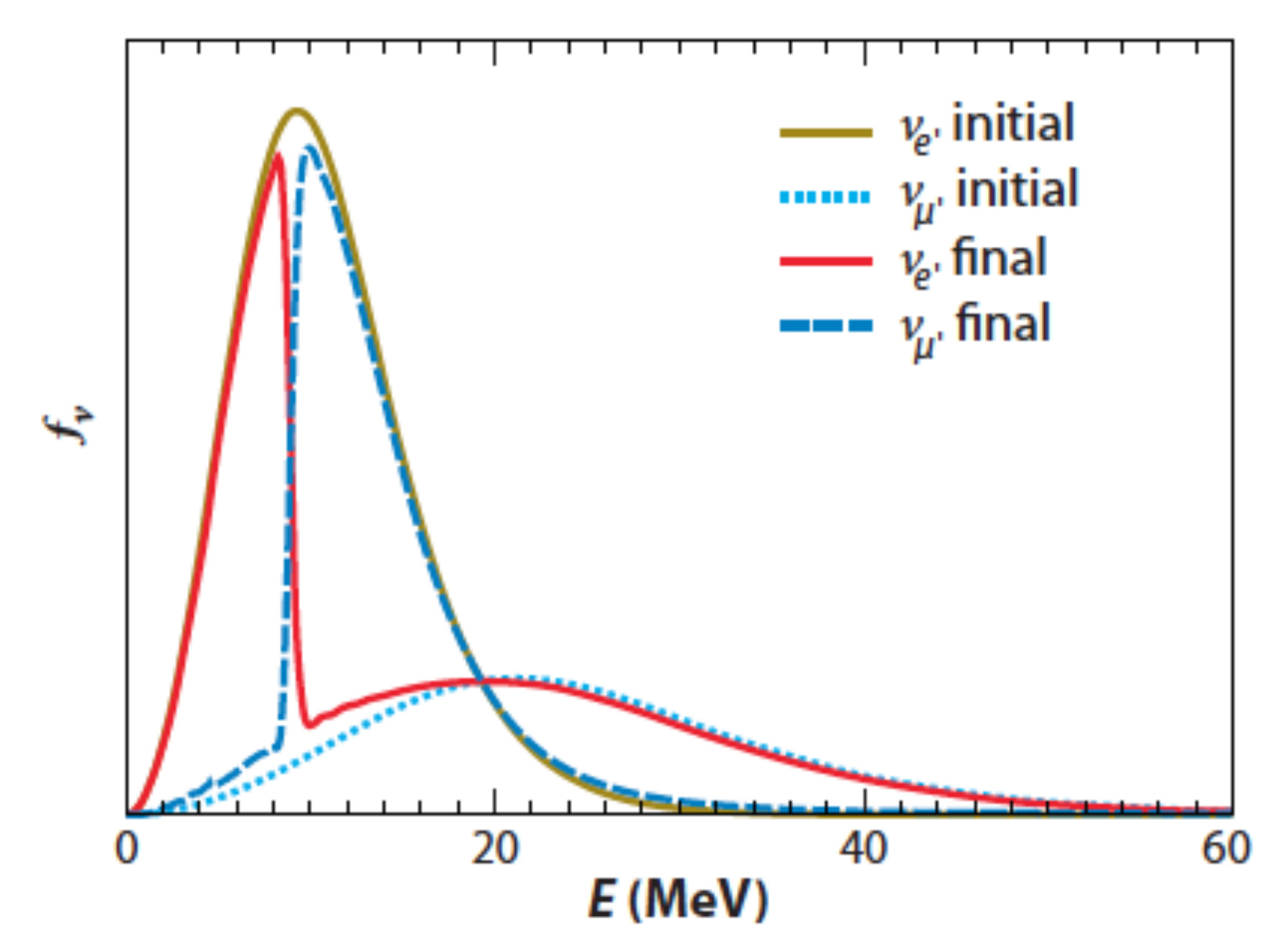
Figure 13: Spectral splits in the bulb model: example of the neutrino spectral swapping in supernovae. Due to $\nu\nu$ interactions, the initial (quasi-thermal) $\nu_{\_}e$ and $\nu_{\_}{\mu}$ spectra undergo significant modification. As the figure shows, there is a critical energy ($E_{\_}{\rm crit}=8$ MeV) for which, if $E<E_{\_}{\rm crit}$ the $\nu_{\_}e$ flux is unchanged, whereas for $E>E_{\_}{\rm crit}$ the $\nu_{\_}x$ and the $\nu_{\_}e$ fluxes interchange. (Figure adapted from [191]).

Other approaches to these phenomena brought further insight. Using the matter basis, Galais et al. [236] found that with the $\nu\nu$ refraction the adiabaticity parameters depend on the matter angle and phase derivative and bipolar oscillations start when the latter diverges. Moreover, Galais and Volpe [238] showed that spectral splits arise from a magnetic resonance phenomenon: the swapping emerges because the spins satisfy (or do not satisfy) a magnetic resonance condition, depending on the neutrino energy.

Pehlivan et al. [406] used a different angle of attack. With an algebraic many-body approach and the Bethe ansatz, they demonstrated that the splits emerged in the transition from a quasi-particle to a particle description. In a subsequent study Pehlivan et al. [407] established that the emergence of spectral splits in the bulb model, when going from the regions where neutrinos strongly interact to those where they weakly interact, is similar to the behavior of Cooper pairs in the BEC-BCS crossover in experiments with ultra cold atomic gases (Fig. 14, see Section III.G).

While first studies revealed instabilities only in inverted mass ordering, Dasgupta et al. [167] showed that more plausible ratios of the $\nu_{\_}e,\bar{\nu}_{\_}e,\nu_{\_}x$ fluxes (i.e. different from one) produced single and multiple spectral splits in both hierarchies. One of the key hypothesis of the bulb model is that neutrinos are emitted as pure flavor states at the neutrinosphere assumed as a sharp surface. Hansen and Smirnov [272] pointed out that if one takes into account that neutrino emission is over a region of finite width (a few kms), the integration over the extended emission region either modifies the growth of slow modes (started in the emission region), or delay the start of flavor transitions.

Moreover, Esteban-Pretel et al. [204] argued that large matter densities introduced decoherence in multi-angle calculations because of the angular factor $(1-\hat{\bf p}\cdot\hat{\bf p}^{\prime})$ in Eq.(15). Following these findings, Chakraborty et al. [137, 136] showed, using one-dimensional supernova simulations, that matter suppressed collective effects when the matter exceeded the $\nu\nu$ number density. This finding should be confirmed by multi-angle calculations using multi-dimensional supernova simulations.

The studies assumed stationarity and homogeneity of the medium where neutrinos propagate. Moreover, they used the mean-field approximation and neglected collisions. Thanks to these approximations, the full 7-dimensional problem of neutrino flavor evolution reduces to a more tractable one, typically in two- or three-dimensions, i.e. ($E,r$) or ($E,r,\theta$). But even schematic models with a reduced number of degrees of freedom are often quite challenging to solve.

A step towards higher spatial dimensionality was provided by the so-called neutrino line model with two spatial dimensions, either with only two neutrino beams from each initial condition [193], or with multi-angles at each point source [7], showing inhomogeneous modes located at larger neutrino densities than homogenous ones. Abbar and Duan [5] and Dasgupta and Mirizzi [168] identified temporal instabilities arising in non-stationary models since time can cancel a (albeit) constant matter term, producing instabilities (quite) deep in the supernova.

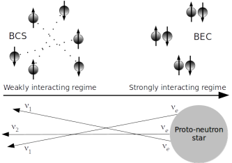
Figure 14: Neutrino-neutrino interactions in a supernova: correspondence between neutrinos propagating from dense to dilute regions and the BEC to BCS limits in ultra cold atomic gases. (Figure from [407]).

Moreover, Cherry et al. [148, 149] uncovered that a neutrino halo – a small amount of back-scattered neutrinos due to collisions – could completely reshape the flavor patterns produced by forward scattering. This finding cast doubts on the treatment of $\nu\nu$ interactions, showing limitations of the mean-field equations used (see Section II.1) in which neutrinos forward scatter only from the neutrinosphere (see Sections III.2 and F). The halo effect was further studied by Sarikas et al. [443] and Cherry et al. [150].

Furthermore, based on a linearized study of the bulb model Raffelt et al. [421] found azymuthal-angle-instabilities. This finding showed that solutions do not necessarily inherit the symmetries of the initial or boundary conditions (unless enforced). This fact was dubbed spontaneous symmetry breaking. Several works confirmed symmetry breaking solutions with linearized analysis in supernovae [365, 140].

Flavor evolution can even reveal chaotic behaviors. This was mentioned by Raffelt and de Sousa Seixas [422] in a stationary model with two opposite neutrino momenta. And, in fact, in the same model Hansen and Hannestad [269] clearly identified the exponential divergence of Liapounov exponents when considering infinitely close initial trajectories of the neutrino spin vectors.

So, after the discovery of novel phenomena in the bulb model, models increased in complexity and included e.g. non-stationarity, inhomogeneities, unconstrained symmetries and more. These in-depth investigations kept uncovering new features and the richness of flavor evolution in dense media, due to the $\nu\nu$ refraction. While theorists thought they were shaping a solid understanding, fast modes arrived ”on the stage”, triggering another ”runaway” of studies …

II.7.2 Fast modes

In a $3\nu$ two-beam model Sawyer [447, 448] found that $\nu\nu$ interactions could ”speed-up” flavor transformation and produce counterintuitive modifications on a short time scale of $t=(2\sqrt{2}G_{\_}{\rm F}n_{\_}{\nu})^{-1}$ of order a few ns. Much later Sawyer [449] considered non-trivial angular distributions at the neutrinospheres, with $\bar{\nu}_{\_}e$ emitted deeper than $\nu_{\_}e$. He identified modes with (tens of) meters scale.

Sawyer’s findings triggered excitement again: fast modes took place close to the neutrinosphere. They could influence the supernova dynamics and nucleosynthesis. Theorists had found the short scale modes they were looking for, finally!

Contrarily to slow modes, fast modes have the peculiarity that they are not triggered neither by the mixings Eqs.(II) and (4), nor by the matter contribution Eq.(9). Since only the neutrino emission matters, Izaguirre et al. [289] introduced the angle distribution of the electron lepton number (ELN) which for $2\nu$ flavors reads

$$G_{\_}{\bf v}=\sqrt{2}G_{\_}{\rm F}\int_{\_}0^{\infty}dE~{}{E^{2}\over{2\pi^{2}}}~{}[\phi_{\_}{\nu_{\_}e}(E,{\bf v})-\phi_{\_}{\bar{\nu}_{\_}e}(E,{\bf v})]\ .$$ (33)

As indicated by the results of Sawyer [449] and pointed out by Dasgupta et al. [169], Izaguirre et al. [289], fast modes take place when the angular distributions of $\nu_{\_}e$ and $\bar{\nu}_{\_}e$ cross each other along a given direction (i.e. $G_{\_}{\bf v}$ changes sign): this is an ELN crossing. The sufficiency of this condition and/or its necessity have been controversial.Morinaga [370] gave the mathematical proof that in inhomogeneous media the occurrence of an ELN crossing is equivalent to the existence of a fast instability, i.e. the condition is both necessary and sufficient. Besides Fiorillo and Raffelt [214] also proved that it is a sufficient condition when the medium is homogenous.

In the last years many studies of fast modes have been realized based on the linearized approach (see for example [127, 9, 8, 180, 478, 6, 134, 138, 139, 458, 391, 514, 247, 519] and Tamborra and Shalgar [482] for a review).

It was already advocated by Sawyer [447] that fast modes could bring flavor equilibration of the different neutrino species. The ansatz has been admitted in the literature for some time. In fact it has the advantage that it simplifies the problem since the neutrino spectra emerge identical from a supernova. However, in a two-beam model, Abbar and Volpe [11] evolved for the first time fast modes in the full non-linear regime showing they do not necessarily lead to flavor equilibration.

Fast modes behave differently in $3\nu$ flavors with respect to $2\nu$ flavors. For the former the concept of ELN crossing needs to be generalized to $\mu$LN and $\tau$LN crossings. Chakraborty and Chakraborty [134] first investigated such effects with the dispersion relation treating both time and space. The authors pointed out the importance of three-flavor effects. The further analysis of Capozzi et al. [126], that went up to the non-linear regime, showed instabilities over tens of ns scale which were either absent (in $2\nu$ flavors), or got damped. Clearly these findings emphasize the need for three-flavor analysis of fast modes.

Since the scale for fast modes is so short, there can be regions requiring the treatment of flavor mechanisms and collisions when the medium is very dense. Indeed the fast rate exceeds the collision rate even within a supernova core. Using a one-dimensional model, with two momentum modes, Capozzi et al. [128] analyzed the interplay between collisions and fast modes and showed that collisions can trigger the conditions for fast conversions. Significant efforts are made to study flavor conversion modes in presence of collisions (see for example Capozzi et al. [128], Richers et al. [429], Hansen et al. [271], Xiong et al. [520], Johns [293], Padilla-Gay et al. [392])). It is necessary to keep in mind, though, that a consistent treatment in multidimensional simulations is numerically very challenging and therefore far ahead.

Fast modes are present in schematic models, but do they occur in detailed supernova simulations? The first investigation by Tamborra et al. [479], based on one-dimensional simulations, concluded for the absence of fast modes. Searches in multidimensional simulations revealed the presence of fast modes, in contrast with this early finding.

Abbar et al. [9] identified fast-growing modes in two- and three-dimensional simulations when $\alpha=n_{\_}{\nu_{\_}e}/n_{\_}{\bar{\nu}_{\_}e}$ is of the order of 1. A linear stability analysis confirmed the presence of fast modes in correspondence with the angular crossings (Fig. 15), even deep in the supernova core. Their influence on the neutrino spectra was found to be small, since the neutrino spectra are already very similar at the location of the crossings.

Glas et al. [254] and Delfan Azari et al. [181] also found ELN crossings nearby the neutrinosphere and confirmed the presence of fast modes in detailed supernova simulations (with full Boltzmann transport) in three- and two-dimensions respectively. It is to be noted that multi-dimensional supernova simulations do not provide full information of the neutrino angular distributions as a function of time. Therefore methods have been developed, as in Dasgupta et al. [170], to identify fast modes using the moments of the angular distributions.

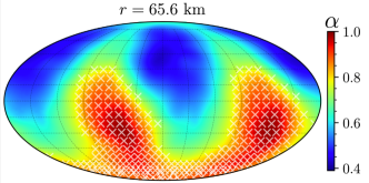
Figure 15: Fast modes in multidimensional supernova simulations: Mollweide projection of the $\bar{\nu}_{\_}e$-over-$\nu_{\_}e$ ratio at a distance $r=65.6$ km in a snapshot at post-bounce time of 200 ms of a 3D supernova model. The white crosses indicate the location where fast modes occur, based on a linearized analysis. (Figure from [9]).

Moment methods are commonly used in supernova codes with classical (Boltzmann) neutrino transport. They require a truncation of the tower of moment equations and the use of a closure approximation to estimate the unknown from the evolved moments. Myers et al. [373] suggested a method to study flavor evolution based on quantum moments, i.e. angular moments of the quantum neutrino distributions. In the bulb model setting, the authors showed that calculations with two moments were able to capture features of multi-angle simulations, such as the onset of collective oscillations, sometimes overestimating the coherence. The method was applied to fast modes by Grohs et al. [261] in a three-dimensional simulation of a neutron star merger. The results showed that the method can qualitatively capture some of the aspects of fast modes like their growth rate.

Nagakura and Zaizen [376] proposed a method to investigate fast modes on large scales ($>$ 10 km) in a supernova, by an ad hoc rescaling of the neutrino number density and studying the convergence when its value tends to the one found in physical conditions. Currently first studies are appearing that implement fast modes in detailed one-dimensional [374] or multi-dimensional core-collapse supernova simulations [198]. The goal is to investigate their impact on the heating rates in the gain region and on the explosion dynamics (see Appendix B). While exploring this role is crucial, at this stage and in the light of the approximations done, it is too early to draw conclusions.

Beyond the studies in the supernova context, Wu and Tamborra [514] performed the first analysis of fast modes in accretion disks resulting from binary compact objects mergers. They found the conditions for fast modes to be generically met because of the excess of $\bar{\nu}_{\_}e$s over $\nu_{\_}e$s and of the geometry of such environments.

As for nucleosynthesis, Xiong et al. [519] studied the influence of fast oscillations in neutrino-driven winds in a low and a high mass core-collapse supernova. They showed that partial (or total) flavor equilibration creates more proton-rich conditions ($Y_{\_}e>0.5$) enhancing the $\nu$p process and mass ejection. Wu et al. [515] considered the impact of fast modes on the $r$-process in a neutrino driven wind nearby a black hole remnant from compact binary mergers. Under the approximate assumption of flavor equilibration, fast modes produced an increase of lanthanides (more generally nuclei with A $>$ 130) up to a factor of $10^{3}$, due to the decrease of $Y_{\_}e$, showing a potentially high impact on kilonova light-curves.

On the contrary, in an analysis for an hyper-massive BNS merger remnant, George et al. [247] found lanthanides to be little affected by fast pairwise conversion (under the same flavor equilibration hypothesis). In the disk outflows of an hypermassive neutron star Fernández et al. [210] studied the production of heavy $r$-process elements in the disk outflows of an hyper-massive neutron star and found that the abundance of lanthanides and actinides, important for kilonova opacities, can be modified up to a factor of 2 if fast modes are included (assuming partial or total flavor equilibration).

In conclusion, while studies clearly show that the impact of flavor mechanisms on $r$-process nucleosynthesis is important, further work is needed, also based on more consistent treatments, in order to draw definite conclusions about their role. As for fast modes and their impact, their investigation undergoes a fast development where interesting aspects are being uncovered. Clearly, these short scale modes will keep attracting attention in the coming years.

III Flavor evolution: Theoretical frameworks

Neutrinos propagating in a dense environment constitute a unique, weakly interacting, many-body system. Its description benefits of a lucky situation in some respects, since one does not have to deal with phenomenological interactions as for atomic nuclei, as it has been for long before the advent of ab-initio calculations. It is a specific case also, because theoretical approaches developed for many-body systems need to be extended to relativistic particles with mixings.

The literature is rich with theoretical approaches for the neutrino many-body system (see the review by Volpe [502]). These range from the mean-field and the extended mean-field equations, the linearized equations and a dispersion relation approach to the neutrino quantum kinetic equations, as we shall now see.

III.1 The mean-field approximation

The mean-field constitutes the simplest approximation to describe neutrino propagation in astrophysical environments. Neutrino mean-field equations were derived by several authors [185, 441, 447, 457, 71, 504].

It is common to determine neutrino propagation using the formalisms of Green’s functions, of density matrices, of neutrino (iso)spins, or of neutrino amplitudes. The density matrix formalism is widely used. The $\nu$ and $\bar{\nu}$ one-body densities are defined as

$$\varrho_{\_}{1,ij}({\bf p},h,{\bf p}^{\prime},h^{\prime}) = \langle a^{\dagger}_{\_}j({\bf p}^{\prime},h^{\prime})a_{\_}i({\bf p},h)\rangle\ ,$$

$$\bar{\varrho}_{\_}{1,ij}({\bf p},h,{\bf p}^{\prime},h^{\prime}) = \langle b^{\dagger}_{\_}i({\bf p},h)b_{\_}j({\bf p}^{\prime},h^{\prime})\rangle\ ,$$ (34)

where the quantum expectation value are over the astrophysical or cosmological background; $i,j\in[1,N]$ with $N$ the number of neutrino families. The diagonal elements of the one-body density matrix correspond to the expectation value of the number operator and are the only contributions for particles without mixings. The off-diagonal elements ($i\neq j$) implement coherence due to the mixings. Sometimes it is said that neutrino evolution requires a ”matrix of densities” quoting Sigl and Raffelt [461].

The mean-field approximation consists in replacing a two-body interaction term, which has the form of a quadratic operator ${\cal I}_{\_}1{\cal I}_{\_}2$, by one-body ones as

$${\cal I}_{\_}1{\cal I}_{\_}2\rightarrow{\cal I}_{\_}1\langle{\cal I}_{\_}2\rangle+\langle{\cal I}_{\_}1\rangle{\cal I}_{\_}2+\langle{\cal I}_{\_}1\rangle\langle{\cal I}_{\_}2\rangle\ .$$ (35)

If one takes the charged- or the neutral-current interaction terms of the GWS model, the Hamiltonian is quartic in the creation and annihilation operators. In the mean-field approximation, the Hamiltonian becomes quadratic in the creation and annihilation operators and has the general bilinear form [457]

$$H_{\_}{\rm MF}(t)=\int d{\bf x}\,\bar{\psi}_{\_}{i}(t,{\bf x})\Gamma_{\_}{ij}(t,{\bf x})\psi_{\_}{j}(t,{\bf x}),$$ (36)

where $\Gamma_{\_}{ij}(t,{\bf x})$ is the interaction kernel that depends on the specific interaction terms that one considers. The quantities $\psi_{\_}i$ denote the neutrino field in the mass basis (for the $i$th mass eigenstate)

$$\psi_{\_}{j}(t,{\bf x})=\sum_{\_}h\int_{\_}{p}[u_{\_}j({\bf p},h)a_{\_}j({\bf p},h)e^{-ip\cdot x}+v_{\_}j({\bf p},h)b_{\_}j^{\dagger}e^{ip\cdot x}]\ ,$$ (37)

with $p\cdot x=p^{\mu}x_{\_}{\mu}$ and $u_{\_}j({\bf p},h)$ and ${v_{\_}j(\bf p},h)$ the four-components complex spinors, solution of the Dirac equation. As an example, putting (37) in (36) and taking the case of $\nu_{\_}e$-electron scattering, the interaction kernel reads

$$\Gamma_{\_}{ee}(t,{\bf x})={G_{\_}F\over\sqrt{2}}\gamma^{\mu}(1-\gamma^{5})\langle\bar{\psi}_{\_}e(t,{\bf x})\gamma_{\_}{\mu}(1-\gamma^{5})\psi_{\_}e(t,{\bf x})\rangle\ .$$ (38)

A theoretical framework to treat the evolution of many-body systems is given by the Born and Green [112], Bogoliubov [109], Kirkwood [306], Yvon [528] (BBGKY) hierarchy. First introduced for a non-relativistic many-body system the hierarchy replaces the exact evolution of the quantum many-body system by a hierarchy of integro-differential equations for $n$-body density matrices

$$\rho_{\_}{1\ldots n}=\langle a^{\dagger}_{\_}n\ldots a^{\dagger}_{\_}1a_{\_}1\ldots a_{\_}n\rangle\ ,$$ (39)

If one truncates the hierarchy at different levels, one can derive approximate equations of motion, including the mean-field, extended mean-field and the Boltzmann equation.

The mean-field approximation consists in neglecting the correlated part of the two-body density

$$\rho_{\_}{12}=\rho_{\_}1\rho_{\_}2-c_{\_}{12}\ ,$$ (40)

i.e. setting $c_{\_}{12}=0$, where $\rho_{\_}{12}$ is the two-body density of a generic many-body system, and $\rho_{\_}1$ and $\rho_{\_}2$ are one-body densities for particles 1 and 2. Since only the uncorrelated part is retained, the two particles propagate independently. Thus the full many-body system evolves as made up of independent particles.

In the BBGKY hierarchy the mean-field approximation corresponds to a truncation at the lowest level, neglecting collisions and more generally two-body (and higher order) correlations. Implementing the correlated part of $\rho_{\_}{12}$ (i.e. $c_{\_}{12}\neq 0$), collisions are also included. Thus one gets from the evolution of the full two-body density $\rho_{\_}{12}$ the Boltzmann equation.

Note that a simple way to derive mean-field evolution equations is through the Ehrenfest theorem

$$i\dot{\varrho}_{\_}{1,ij}=\langle[a^{\dagger}_{\_}ja_{\_}i,H]\rangle\ ,$$ (41)

where the neutrino Hamiltonian operator here is in second-quantized form.

While BBGKY was originally for a non-relativistic many-body system, Calzetta and Hu [124] generalized it for relativistic many-body systems which involves, in particular, an infinite hierarchy of equations. Volpe et al. [504] applied the BBGKY hierarchy to a many-body neutrino system, considering neutrino and antineutrino one-body densities (III.1) in an astrophysical environment. The authors obtained the commonly used mean-field equations, as well as extended mean-field equations, as we will discuss (see section III.C). Following these developments, Froustey et al. [232] included also the contribution of $c_{\_}{12}$ and derived the Boltzmann equation for particles with mixings (neutrino quantum kinetic equations) for the case of the early universe.

III.2 The mean-field Hamiltonian: a derivation

Let us consider a particle propagating in a medium and interacting with the particles composing it. The mean-field Hamiltonian associated with a given interaction term depends on a coherent addition of the scattering amplitudes between the propagating particle and a particle in the background. More explicitly, the mean-field potential can be derived from

$$V_{\_}{kr}(\rho)=\sum_{\_}{s,p}v_{\_}{(kp,rs)}\rho_{\_}{sp}\ ,$$ (42)

where the sum (or integration) is over the product of the matrix elements $v_{\_}{(kp,rs)}$ between the incoming and outgoing single-particle states, and the quantity $\rho_{\_}{sp}$ is

$$\rho_{\_}{sp}=\langle a^{\dagger}_{\_}pa_{\_}s\rangle\$$ (43)

where the average is over the background. The quantum numbers $k,p,r,s$ (e.g. the particle momentum and helicity) characterize the incoming and outgoing single-particle states in the scattering process.

Let us now apply Eqs.(42)-(43) to the neutrino case and, as an example, derive the mean-field term of the matter Hamiltonian associated with $\nu_{\_}e$-$e$ scattering (Figure 3, upper right tadpole diagram).

The charged-current interaction term associated with $\nu_{\_}e$-e scatting reads

$$H_{\_}{\rm CC}= {G_{\_}{\rm F}\over{\sqrt{2}}}[\bar{\psi}_{\_}{\nu_{\_}e}(t,{\bf x})\gamma^{\mu}(1-\gamma_{\_}5)\psi_{\_}{e}(t,{\bf x})]$$

$$\times[\bar{\psi}_{\_}{e}(t,{\bf x})\gamma_{\_}{\mu}(1-\gamma_{\_}5)\psi_{\_}{\nu_{\_}e}(t,{\bf x})]\ .$$ (44)

The first step in determining Eq. (42) is to evaluate the matrix elements

$$v_{\_}{(kp,rs)}\equiv\langle k,p|H_{\_}{\rm CC}|r,s\rangle\ .$$ (45)

More explicitly one needs to calculate

$$v_{\_}{(kp,rs)}= {G_{\_}{\rm F}\over{\sqrt{2}}}\langle\nu_{\_}e,e|\int d{\bf x}~{}[\bar{\psi}_{\_}{e}(t,{\bf x})\gamma^{\mu}(1-\gamma_{\_}5)\psi_{\_}{e}(t,{\bf x})]$$

$$\times[\bar{\psi}_{\_}{\nu_{\_}e}(t,{\bf x})\gamma_{\_}{\mu}(1-\gamma_{\_}5)\psi_{\_}{\nu_{\_}e}(t,{\bf x})]|\nu_{\_}e,e\rangle\ ,$$ (46)

where the Fierz transformation has been applied to Eq.(III.2).

By introducing the Fourier expansions of the electron and the neutrino quantum fields Eq.(37), one can calculate the matrix element using the following general relation

$$\langle e(1)|a^{\dagger}(2)a(3)|e(4)\rangle= (2\pi)^{3}\delta^{3}({\bf p}_{\_}1-{\bf p}_{\_}2)2E_{\_}{p_{\_}1}\delta_{\_}{h_{\_}1,h_{\_}2}$$

$$(2\pi)^{3}\delta^{3}({\bf p}_{\_}3-{\bf p}_{\_}4)2E_{\_}{p_{\_}3}\delta_{\_}{h_{\_}3,h_{\_}4}\ ,$$ (47)

that can be easily obtained from the equal-time anti-commutation rules (see Footnote 20). Here the labels (1,2,3,4) stand for a set of single particle quantum numbers (${\bf p},h$). The momentum of the incoming particle is ${\bf p}_{\_}4$ and the one of the outgoing particle is ${\bf p}_{\_}1$.

Using (III.2) one gets

$$v_{\_}{({\bf k}^{\prime}{\bf p}^{\prime},{\bf k}{\bf p})}= {G_{\_}{\rm F}\over{\sqrt{2}}}\int d{\bf x}~{}[\bar{u}_{\_}{\nu_{\_}e}({\bf k}^{\prime})\gamma^{\mu}(1-\gamma_{\_}5)u_{\_}{\nu_{\_}e}({\bf k})]$$

$$\times[\bar{u}_{\_}{e}({\bf p}^{\prime})\gamma_{\_}{\mu}(1-\gamma_{\_}5)u_{\_}{e}({\bf p})]e^{i({\bf p}+{\bf k}-{\bf p}^{\prime}-{\bf k}^{\prime})\cdot{\bf x}}\ ,$$ (48)

where $({\bf p},{\bf k})$ and $({\bf p}^{\prime},{\bf k}^{\prime})$ are the momenta of the incoming and outgoing particles respectively. The first two factors in the integral depend on spinorial products, whereas the last one ensures momentum conservation.

The second step to determine the mean-field term is to perform the integration over the degrees of freedom of the electron background and evaluate

$$V_{\_}{\rm CC}(n_{\_}e)= {G_{\_}{\rm F}\over{\sqrt{2}}}\sum_{\_}{h_{\_}e,h_{\_}e^{\prime}}\int_{\_}{p_{\_}e,p^{\prime}_{\_}e}\int d{\bf x}~{}[\bar{u}_{\_}{\nu_{\_}e}({\bf k}^{\prime})\gamma^{\mu}(1-\gamma_{\_}5)u_{\_}{\nu_{\_}e}({\bf k})]$$

$$\times[\bar{u}_{\_}{e}({\bf p}^{\prime})\gamma_{\_}{\mu}(1-\gamma_{\_}5)u_{\_}{e}({\bf p})]e^{i({\bf p}+{\bf k}-{\bf p}^{\prime}-{\bf k}^{\prime})\cdot{\bf x}}$$

$$\times\rho_{\_}{({\bf p}_{\_}e,h_{\_}e,{\bf p}_{\_}e^{\prime},h_{\_}e^{\prime})}\ ,$$ (49)

with

$$\rho_{\_}{({\bf p}_{\_}e,h_{\_}e,{\bf p}_{\_}e^{\prime},h_{\_}e^{\prime})} =\langle\psi|a^{\dagger}_{\_}e({\bf p}_{\_}e^{\prime},h_{\_}e^{\prime})a_{\_}e({\bf p}_{\_}e,h_{\_}e)|\psi\rangle\,.$$ (50)

Here the expectation value is over the wave-function describing the background (at finite temperature $T$ and chemical potential $\mu$).

If one assumes that the background particles are uncorrelated (independent), then the expectation value can be performed on the single-particle states describing the electrons. Besides neglecting correlations, one very often makes the following ansatz for the background

$$\rho_{\_}{({\bf p}_{\_}e,h_{\_}e,{\bf p}_{\_}e^{\prime},h_{\_}e^{\prime})} =(2\pi)^{3}\delta^{3}({\bf p}_{\_}e-{\bf p}_{\_}e^{\prime})\delta_{\_}{h_{\_}e,h_{\_}e^{\prime}}2E_{\_}{p}\rho_{\_}{e,p}\ ,$$ (51)

that is, that the medium is homogeneous and only forward-scattering is considered, the electrons (and therefore neutrino) momenta are unchanged. The quantity $\rho_{\_}{e,p}$ is the distribution of the electron occupation numbers which follows a Fermi-Dirac function. We often say that the mean-field approximation corresponds to coherent forward scattering.

By plugging Eq.(51) into Eq. (III.2), the spinorial products in Eq. (III.2) can be evaluated thus giving

$$8p^{\mu}(k_{\_}{\mu}-ms_{\_}{\mu})=8E_{\_}{p}E_{\_}{k}(1-\hat{\bf p}\cdot\hat{\bf k})(1-h_{\_}{\nu})\ ,$$ (52)

where we have introduced the 4-vector

$$s_{\_}{\mu}=h_{\_}{\nu}\Big{(}{|{\bf k}|\over{m}},{E_{\_}{k}\over{m|{\bf k}|}}\Big{)}\ ,$$ (53)

and already imposed momentum conservation. Assuming that electrons are relativistic, one gets

$$V_{\_}{\rm CC}(n_{\_}{e})= {G_{\_}{F}\over{\sqrt{2}}}(2\pi)^{3}\delta^{3}({\bf k}-{\bf k}^{\prime})8E_{\_}{k}(1-h_{\_}{\nu})\int_{\_}{p}(1-\hat{\bf p}\cdot\hat{\bf k})\rho_{\_}{e,p}\ ,$$

$$= 2a\sqrt{2}G_{\_}{\rm F}\int{{d{\bf p}}\over{(2\pi)^{3}}}(1-\hat{\bf p}\cdot\hat{\bf k})\rho_{\_}{e,p}\ ,$$ (54)

with $a=(2\pi)^{3}\delta^{3}({\bf k}-{\bf k}^{\prime})E_{\_}{k}(1-h_{\_}{\nu})$. If the medium is isotropic the angular dependence in Eq.(III.2) averages out.

Since the total number of electrons in the medium is given by

$$N_{\_}e\equiv \sum_{\_}{h_{\_}e}\int_{\_}{p}\langle a^{\dagger}_{\_}e({\bf p},h_{\_}e)a_{\_}e({\bf p},h_{\_}e)\rangle=2V\int{d{\bf p}\over{(2\pi)}^{3}}\rho_{\_}{e,p}\ ,$$ (55)

equation (III.2) becomes

$$V_{\_}{\rm CC}(n_{\_}e)=\sqrt{2}G_{\_}{\rm F}n_{\_}e\ ,$$ (56)

where ${n}_{\_}e=N_{\_}e/V$ is the electron number density. This is the well known mean-field Hamiltonian responsible for the MSW effect in matter Eq. (7).

Let us consider a $\bar{\nu}$ propagating in an electron background. Using the same procedure, the derivation of the mean-field contribution requires the calculation of the matrix element Eq.(III.2) involving this time the $b$ and $b^{\dagger}$ operators. This introduces a negative sign arising from anti-commuting the antiparticle operators. Then, one gets the well known potential

$$V_{\_}{\rm CC}(n_{\_}e)=-\sqrt{2}G_{\_}{\rm F}n_{\_}e\ ,$$ (57)

with an opposite sign with respect to the neutrino case. Similarly, one can obtain that the potential for $\bar{\nu}_{\_}e$-positron ($\nu_{\_}e$-positron) scattering has a positive (negative) sign respectively.

Following the procedure just outlined, one can derive any mean-field contribution to the neutrino Hamiltonian, such as the those coming from $\nu\nu$ interactions, or from NSI.

III.3 Beyond the usual mean-field

The mean-field equations Eqs.(14) and (17) with vacuum mixings, the standard charged- and neutral-current $\nu$-matter and $\nu\nu$ interactions respectively have been widely used in studies of flavor evolution in dense astrophysical environments. Already more than a decade ago, some works explored extensions of such equations to establish the robustness of the mean-field approximation and the possible necessity to go beyond.

Let us first mention that, as was pointed out by several authors, the Hamiltonian with $\nu\nu$ interactions is analogous to an interacting system of spins that have a spin-exchange interaction and feel an external magnetic field. Following Balantekin and Pehlivan [71], one can introduce the operators

$$J^{+}_{\_}{\bf p} =a_{\_}x^{\dagger}({\bf p})a_{\_}e({\bf p})~{}~{}J^{-}_{\_}{\bf p}=a_{\_}e^{\dagger}({\bf p})a_{\_}x({\bf p})$$ (58)

$$J^{0}_{\_}{\bf p} =\frac{1}{2}\left[a_{\_}x^{\dagger}({\bf p})a_{\_}x({\bf p})-a_{\_}e^{\dagger}({\bf p})a_{\_}e({\bf p})\right]\ ,$$

that satisfy the commutation relations

$$[J^{0}_{\_}{\bf p},J^{\pm}_{\_}{\bf p}] =\pm\delta^{3}({\bf p}-{\bf q})J^{\pm}_{\_}{\bf p}$$ (59)

$$[J^{+}_{\_}{\bf p},J^{-}_{\_}{\bf q}] =2\delta^{3}({\bf p}-{\bf p})J^{0}_{\_}{\bf p}\ ,$$

and are the generators of as many SU(2) algebra(s) as the number of distinct neutrino momenta.

The neutrino Hamiltonian for 2$\nu$ can be written as [71, 406]

$$H =\sum_{\_}{\omega}\omega{\rm{\bf B}}_{\_}{\rm vac}\cdot{\bf J}_{\_}{\omega}+\mu\sum_{\_}{{\bf p},{\bf q}}(1-\cos\theta_{\_}{{\bf p}{\bf q}}){\bf J}_{\_}{\bf p}\cdot{\bf J}_{\_}{\bf q}\ .$$ (60)

The first term is the vacuum contribution that depends the effective vacuum magnetic field ${\bf B}_{\_}{\rm vac}$ (see Appendix A) and on ${\bf J}_{\_}{\omega}$, the flavor (iso)spin operator of the neutrino with the vacuum oscillation frequency $\omega$. The second term is the $\nu\nu$ interaction term in the mean-field approximation, where neutrinos either keep or exchange their momenta. The $\nu\nu$ coupling is $\mu=\sqrt{2}G_{\_}{\rm F}/V$, $\theta_{\_}{{\bf p}{\bf q}}$ the angle between ${\bf p}$ and ${\bf q}$. Here the matter term is neglected.

Balantekin and Pehlivan [71] provided a derivation of the mean-field equations using the algebraic formulation of the neutrino Hamiltonian (60). The authors used a coherent-state path-integral approach and showed that the mean-field equations correspond to the saddle point approximation of the path-integral for the full many-body system. Moreover, they pointed out contributions beyond the mean-field as corrections to the saddle-point solution.

Later on Volpe et al. [504] used the BBGKY hierarchy to derive mean-field equations for the $\nu$ and $\bar{\nu}$ one-body density matrices Eqs.(III.1) in a dense astrophysical environment. Moreover, thanks to the hierarchy, the authors pointed out that the neutrino evolution equations had further terms at the mean-field level, namely two-point correlators from wrong-helicity contributions due to neutrino masses and from pairing (or abnormal) densities. For Dirac neutrinos the latter read

$$\kappa_{\_}{ij}(t,{\bf q},h,{\bf q}^{\prime},h^{\prime}) =\langle b_{\_}{j}(t,{\bf q^{\prime}},h^{\prime})a_{\_}{i}(t,{\bf q},h)\rangle\ ,$$ (61)

and their hermitian conjugates. Volpe et al. [504] showed that in presence of pairing correlators one can cast the extended mean-field evolution equations, similarly to Eq. (14) as

$$i\dot{\cal R}=[{\cal H},{\cal R}]\ ,$$ (62)

by introducing the quantities ${\cal H}$ and ${\cal R}$ that are the generalized Hamiltonian and density. These includes both the $\nu$ and $\bar{\nu}$ contributions and have a to $2N\times 2N$ matrix form (see Volpe et al. [504] for their explicit expressions). Such a system of $\nu$ and $\bar{\nu}$, with pairing correlators, can be described in terms of independent quasi-particles, by introducing a Bogoliubov transformation Väänänen and Volpe [491].

Besides pairing correlators, wrong helicity contributions have also been discussed. Already in the early nineties, Rudzsky [437] had derived quantum kinetic equations for Wigner distribution functions and included both neutrino flavor and spin. In their derivation of neutrino quantum kinetic equations, Vlasenko et al. [496] pointed out again contributions from the correlators

$$\zeta_{\_}{ij}(t,{\bf q})=\langle a^{\dagger}_{\_}j(t,{\bf q},+)a_{\_}i(t,{\bf q},-)\rangle\ ,$$ (63)

and named them spin coherence. They are due to the neutrino mass and suppressed by the factor $m/E$.

Serreau and Volpe [457] derived the most general mean-field equations for inhomogeneous and anisotropic media considering Dirac as well as Majorana neutrinos. Such equations include contributions either from pairing or from wrong-helicity correlators referred to as helicity (instead of spin) coherence. Using the approach of Serreau and Volpe [457], Kartavtsev et al. [298] also included contributions from neutrino electromagnetic properties.

Spin or helicity coherence requires anisotropy of the medium to be non-zero. The corresponding generalized equations (62) can again be cast in the form Eq.(14) but with the generalized Hamiltonian having both flavor and helicity structure [437, 496, 457]. Helicity coherence couples $\nu$ with $\bar{\nu}$, i.e. active and sterile neutrinos if $\nu$ are Dirac particles, or neutrinos and antineutrinos if $\nu$ are Majorana particles.

The impact on flavor evolution of the supplementary terms from the correlators (61) and (63) was investigated as well. Kartavtsev et al. [298] pointed out that the pairing correlators do not influence flavor because the large kinetic contributions cannot be removed. This fact makes the influence of the off-diagonal contributions from pairing correlators tiny.

Concerning helicity coherence, simulations in $3\nu$ flavors with detailed astrophysical inputs from binary neutron star merger remnants [143] or supernovae [484] showed that non-linear feedback does not operate in detailed settings (see section II.F.2). As a consequence, according to current understanding, helicity coherence does not seem to influence the neutrino flavor in media.

III.4 Linearization

Linearization is a widespread approach. It is used in many domains of physics, e.g. in nuclear physics, condensed matter or in hydrodynamics. In the linearization procedure, which is a small amplitude approximation, one solves eigenvalue equations that are numerically more tractable than the full non-linear problem.

The first application of linearization to the neutrino mean-field equations in a supernova was done by Sawyer [448]. Afterwards, Banerjee et al. [79] derived a linearized version of the equations of motion in the bulb model. Since then, the procedure has been widely employed in the study of both slow and fast modes. Väänänen and Volpe [491] provided an alternative derivation of the linearized equations, by generalizing the random-phase-approximation (RPA) commonly used in the study of atomic nuclei or metallic clusters. Subsequently Izaguirre et al. [289] recast the linearized equations in a dispersion relation approach.

III.4.1 The linearised equations

Let us have a closer look at the linearized version of the equations of motion for supernova neutrinos. Here we follow Banerjee et al. [79] and consider the bulb model, which includes neutral-current $\nu\nu$ interactions (section II.G.1). For 2$\nu$ flavors, the neutrino flux matrices can be rewritten as

$$\rho_{\_}{\ell,r}={\phi_{\_}{\nu_{\_}e,\ell,r}+\phi_{\_}{\nu_{\_}x,\ell,r}\over 2}+g_{\_}{\ell}\Big{(}\begin{tabular}[]{cc}$s_{\_}{\ell,r}$&$S_{\_}{\ell,r}$\\ $S^{*}_{\_}{\ell,r}$&- $s_{\_}{\ell,r}$\\ \end{tabular}\Big{)}\ ,$$ (64)

where $\ell=({\omega,u})$. The last matrix on the r.h.s., referred to as ${\bf S}_{\_}{\ell,r}$ is an Hermitian matrix and its pre-factor

$$g_{\_}{\ell}={(\phi^{0}_{\_}{\nu_{\_}e,\ell}-\phi^{0}_{\_}{\nu_{\_}x,\ell})\over 2}\ .$$ (65)

depends on the fluxes at the neutrinosphere. The $s_{\_}{\ell,r}$ factor tells, for a given mode, how much the flavor content has changed with respect to the initial condition. The elements of ${\bf S}_{\_}{\ell,r}$ satisfy the normalization condition $s^{2}_{\_}{\ell,r}+|S_{\_}{\ell,r}|^{2}=1$. The quantities $(1+s)/2$ are the survival probabilities.

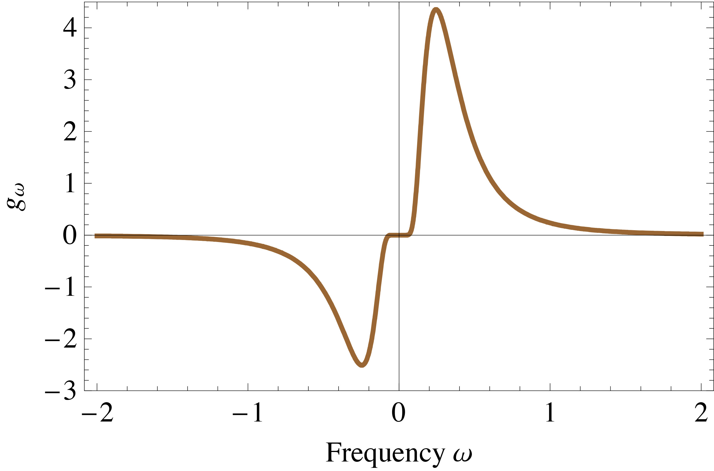
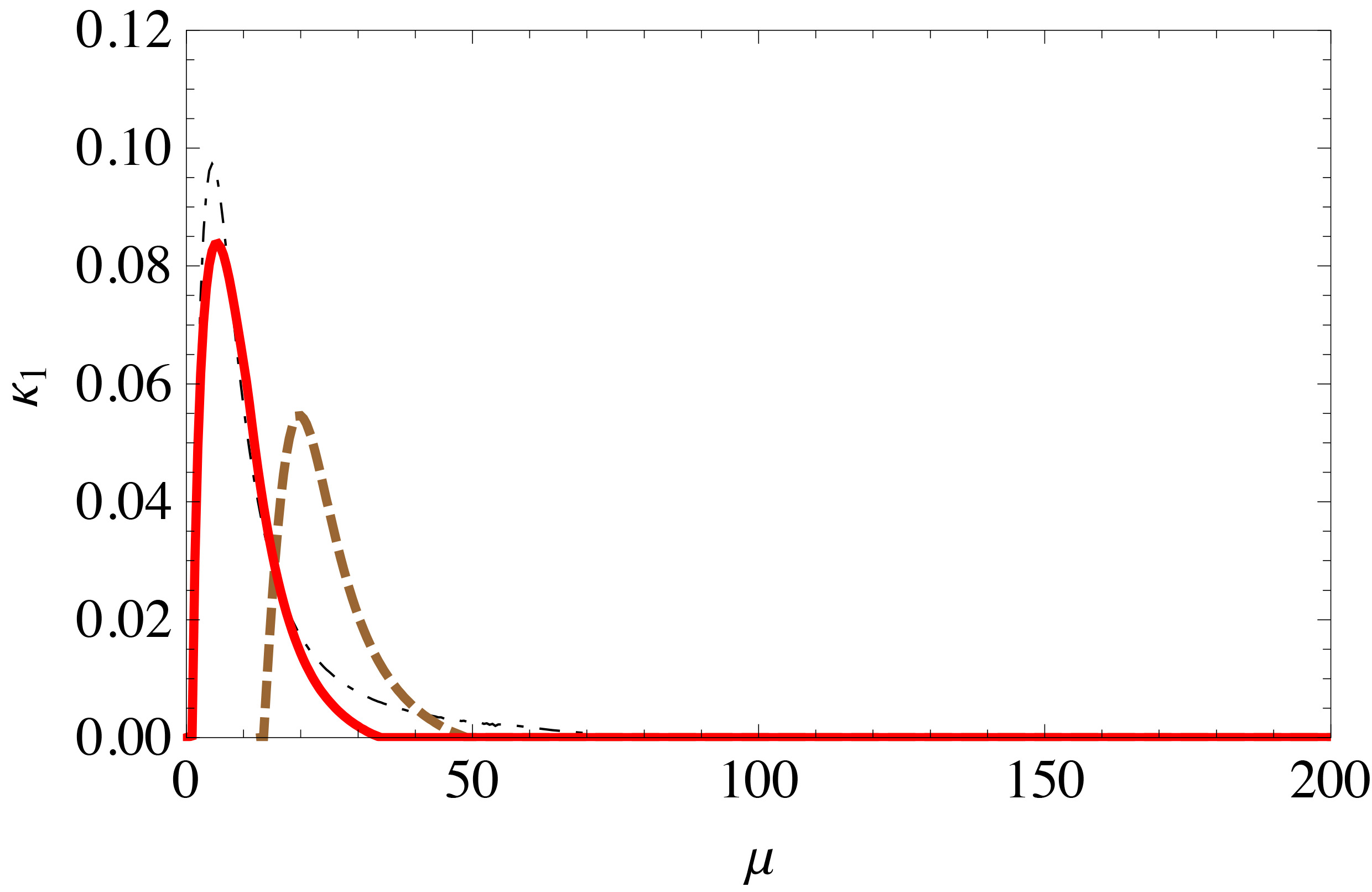
Figure 16: Linearisation: example of the solution of the eigenvalue equations for neutrino Fermi-Dirac distributions at the neutrinosphere (upper figure). The positive frequencies correspond to neutrinos, whereas the negative ones to antineutrinos. The quantity $\kappa_{\_}1$, as a function of the $\nu\nu$ interaction coupling constant $\mu$, is the imaginary part of one of the two unstable solutions (lower figure). (Figure adapted from Banerjee et al. [79].)

The indices $(\omega,u,r)$ are the vacuum oscillation frequency, $u=\sin^{2}\vartheta_{\_}R$ with $u\in[0,1]$ characterizes the neutrino emission at the neutrinosphere (at $r=R$), $r$ is the distance defining the $\nu\nu$ intersection point along the symmetry direction (Fig. 12).

In the linearization procedure one considers the initial state and performs small variations around it. The initial states at the neutrinosphere are in our case ${\bf S}_{\_}{\ell,R}={\rm diag}(1,-1)$ and $\rho_{\_}{\ell,R}={\rm diag}(\phi^{0}_{\_}{\nu_{\_}e},\phi^{0}_{\_}{\nu_{\_}x})$ Eq. (64). The small amplitude approximation consists in the following assumption

$$s_{\_}{\ell,r}\simeq 1~{}~{}~{}~{}|S_{\_}{\ell,r}|\ll 1.$$ (66)

Under this hypothesis, the neutrino mean-field equations Eq.(14) with the contributions from vacuum Eq. (4), matter Eq. (9), and $\nu\nu$ interaction Eq. (15) become, when $r\gg R$

$$i\partial_{\_}rS_{\_}{\ell,r}=~{} [\omega~{}+~{}u(\lambda_{\_}r~{}+~{}\epsilon\mu_{\_}r)]~{}S_{\_}{\ell,r}$$

$$-\mu_{\_}r\int_{\_}0^{1}du^{\prime}\int_{\_}{-\infty}^{+\infty}d\omega^{\prime}(u+u^{\prime})g_{\_}{\ell^{\prime}}S_{\_}{\ell^{\prime},r}\ .$$ (67)

with the positive (negative) frequencies corresponding to neutrinos (antineutrinos) (see Figure 16). In Eq.(III.4.1) the third term on the r.h.s. is the total lepton number $\epsilon=\int~{}du~{}d\omega~{}g_{\_}{\ell}$ (normalized to $\phi^{0}_{\_}{\bar{\nu}_{\_}e}$). The second and the last terms on the r.h.s. are the matter and the $\nu\nu$ terms, with the following coefficients

$$\lambda_{\_}r=\sqrt{2}G_{\_}{\rm F}(n_{\_}e-n_{\_}{\bar{e}}){R^{2}\over{2r^{2}}}~{}~{}~{}\mu_{\_}r={\sqrt{2}G_{\_}{\rm F}\phi^{0}_{\_}{\bar{\nu}_{\_}e}R^{2}\over{8\pi r^{4}}}\ .$$ (68)

One seeks for solutions of Eq. (III.4.1) of the type

$$S_{\_}{\ell,r}=Q_{\_}{\ell,r}e^{-i\Omega r}\ ,$$ (69)

which leads to the eigenvalue equations

$$[\omega~{}+~{}u(\lambda_{\_}r~{}+~{}\epsilon\mu_{\_}r)- \Omega]Q_{\_}{\ell,r} =$$

$$-\mu_{\_}r\int_{\_}0^{1}du^{\prime}\int_{\_}{-\infty}^{+\infty}d\omega^{\prime}(u+u^{\prime}) g_{\_}{\ell^{\prime}}Q_{\_}{\ell^{\prime},r}\ .$$ (70)

If the eigenvalue $\Omega\in{\Re}$, the initial condition is stable and the system performs small oscillations around it. If $\Omega\in{\cal C}$, one faces an instability in flavor space: the system deviates exponentially from the initial state. This is often called a runaway solution. Figure 16 gives an example of the application of linearized equations in the supernova context.

Therefore, a complex eigenvalue indicates the start of flavor modification when neutrinos depart from the neutrinosphere. However, it is worth emphasizing that linearization does not provide any information on the full non-linear regime. Indeed the linearized equations are inherently based on the small amplitude approximation Eq.(66). Only the full numerical solution of the equations of motion tells us how significant flavor conversion is, at large scales.

In the study of atomic nuclei or metallic clusters, linearized equations are obtained with RPA. With this approach one determines small variations of the matter density around the initial state. If the eigenvalues are real that indicates that the initial state is a true ground state; if they are complex, then the initial state is not a ground state of the system. The latter situation is, in fact, what one looks for, in the neutrino case. Also, in RPA, one can face ”spurious” solutions that are numerical artifacts (see for example [430]). These were also found in the neutrino context e.g. when multi-angle calculations of the $\nu\nu$ interaction do not include a sufficiently large number of angle bins [442].

Here is how Väänänen and Volpe [491] generalized RPA to neutrinos. At initial time, the density matrices $\varrho$ and $\bar{\varrho}$ correspond to a stationary state

$$[h^{0},\varrho^{0}]=0~{}~{}~{}~{}~{}~{}[\bar{h}^{0},\bar{\varrho}^{0}]=0\ .$$ (71)

Since RPA is a small amplitude approximation, one performs small variations $\delta\varrho(t)$ of the density around $\varrho^{0}$:

$$\delta\varrho=\varrho^{0}+\delta\varrho(t)=\varrho^{0}+\varrho^{\prime}e^{-i\Omega t}+\varrho^{\prime\dagger}e^{i\Omega^{*}t}.$$ (72)

where $\varrho^{\prime}$ here stands for the off-diagonal terms of the density matrix. The mean-field Hamiltonian around this solution changes accordingly

$$h(\varrho)=h^{0}+{\delta h\over{\delta\varrho}}\Big{|}_{\_}{\varrho^{0}}\delta\varrho+\ldots~{}~{}~{}~{}\bar{h}(\bar{\varrho})=\bar{h}^{0}+{\delta\bar{h}\over{\delta\bar{\varrho}}}\Big{|}_{\_}{\bar{\varrho}^{0}}\delta\bar{\varrho}+\ldots\ .$$ (73)

By implementing Eq. (72) and retaining terms at lowest order, one obtains linearized equations of motion which can be cast in the following matrix form (known in RPA)

$$\left(\begin{array}[]{ll}A&B\\ \bar{B}&\bar{A}\\ \end{array}\right)\left(\begin{array}[]{l}\varrho^{\prime}\\ \bar{\varrho}^{\prime}\\ \end{array}\right) =\Omega\left(\begin{array}[]{l}\varrho^{\prime}\\ \bar{\varrho}^{\prime}\\ \end{array}\right).$$ (80)

Note that linearized equations were also cast in a similar matrix form in Sarikas et al. [442]. The condition for the applicability of linearized equations by Väänänen and Volpe [491] is that the system satisfies Eqs.(71) at initial time. This can hold in the flavor basis, but also in the matter basis. In the latter case, in principle, one could apply the linearized equations also at a time later than the initial time at the neutrinosphere (as usually done).

III.4.2 A dispersion-relation approach

A third formulation of the linearized equations was suggested by Izaguirre et al. [289], for fast modes. The authors cast them in a dispersion-relation approach where the neutrino modes are neutrino flavor (iso)spin waves, described by a four vector $c$ and a ”polarization” vector, in the matter and the neutrino backgrounds. Instead of Eq.(III.4.1) one seeks for plane waves (in an homogeneous and stationary background)

$$S_{\_}{{\bf v}}(t,{\bf r})=Q_{\_}{\bf v}(\Omega,{\bf K})e^{-i(\Omega t-{\bf K}\cdot{\bf r})}\ .$$ (81)

After linearizing the mean-field equations (14), one gets the following equation

$$v^{\mu}k_{\_}{\mu}Q_{\_}{\bf v}=-\int{d{\bf v}\over{4\pi}}v^{\mu}v^{\prime}_{\_}{\mu}G_{\_}{\bf v}Q_{\_}{\bf v^{\prime}}$$ (82)

where $v^{\mu}=(1,{\bf v})$, and $(\Omega,{\bf K})$ is replaced by $(\omega,{\bf k})$. By considering

$$Q_{\_}{\bf v}=a^{\mu}k_{\_}{\mu}/v^{\mu}k_{\_}{\mu}\ ,$$ (83)

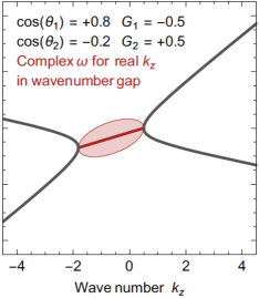
Figure 17: Dispersion-relation approach: results for a two-beam model with angular modes $G_{\_}1$ and $G_{\_}2$. The red region corresponds to complex values of $\omega$ for real ${\bf k}$ with ${\bf k}=(0,0,k_{\_}z)$ for which fast modes grow in time (temporal instability). (Figure adapted from Izaguirre et al. [289].)

one can recast Equation (82) as a dispersion relation $\omega=\omega(k)$ as

$$\Pi^{\mu\nu}a_{\_}{\nu}=0$$ (84)

seeking for non-trivial solutions, such that ${\rm det}[\Pi^{\mu\nu}]=0$. The ”polarisation tensor” in Eq. (84) reads

$$\Pi^{\mu\nu}=\eta^{\mu\nu}+\int{d{\bf v}\over{4\pi}}G_{\_}{\bf v}{v^{\mu}v^{\nu}\over{\omega-{\bf v}\cdot{\bf k}}}\ ,$$ (85)

with $\eta^{\mu\nu}={\rm diag}(+,-,-,-)$. Equation (84) is a quartic equation in $\omega$ whose roots give four possible dispersion-relation branches: a) $(\omega,{\bf k})\in{\Re}$ for stable solutions; b) $\omega$ or ${\bf k}$ $\in{\cal C}$ for an unstable solution that grows in time, or in space (Fig. 17); c) $\omega,{\bf k}\in{\cal C}$, for a mode growing in space and time.

A classification of instabilities was suggested by Capozzi et al. [127] following the one for plasmas by Sturrock [468] and Briggs [116]. According to this classification, the linear instabilities can be of four categories: the completely stable or stable with damping correspond to spatially stable modes; the absolute and convective grow either temporally (but still embracing the point of its origin) or spatially, moving away from its origin while growing in amplitude and extent. Note that many flavor evolution studies (for slow or fast modes) were performed by evolving either space or time.

Among the applications is the study by Martin et al. [353] in a dynamic one-dimensional model. The authors showed that fast modes evolve coherently in the non-linear regime in time and in space, when the corresponding ELN crossings undergo absolute or convective instabilities in the linear regime. The work by Capozzi et al. [127] was further deepened by Yi et al. [523] who pointed out that the complex dispersion relation branches are bounded by critical points and emphasized their usefulness in identifying fast modes.

III.5 Neutrino quantum kinetic equations

The study of the interplay between collisions and flavor modes is numerically challenging. Thus its investigation is still in early stages. First it requires a consistent theoretical framework where one goes from the dense collision-dominated regime to the dilute regions in which mean-field equations are sufficient. Second, the dimensionality remains high in astrophysical environments; whereas in the early universe isotropy and homogeneity reduces the dimensionality of the problem, making it numerically tractable.

Numerous authors derived neutrino quantum kinetic equations (QKEs) for the early universe [466, 437, 461, 356, 496, 106, 232], see also the review by Volpe [502]). Such QKEs are being used for the study of neutrino flavor evolution in dense astrophysical environments.

Rudzsky [437] gave an early derivation of the Boltzmann equation for neutrino Wigner distribution functions including neutrino mixings and the MSW potential. He considered distribution functions as a matrix in the neutrino spin and isospin space, allowing both neutrino oscillations in flavor and spin. The latter become zero when the neutrino rest mass is zero.

Sigl and Raffelt [461] derived QKEs for a matrix of densities for the early universe, implementing antineutrinos for the first time. They included (anti)neutrino scattering on neutrons, protons, electrons, positrons, $\nu$ and pair annihilation in a perturbative approach using the assumption of molecular chaos. In this approximation, the collision timescale is short enough that correlations do not develop between collisions: the incoming and outgoing particles in the collision integrals are free single-particle states.

Vlasenko et al. [496] gave an alternative derivation of the flavored quantum Boltzmann equations for Majorana neutrinos using the Closed Time Path (or ”in-in”) formalism and the 2 Particle-Irreducible (2PI) effective action. Blaschke and Cirigliano [106] extended their results and obtained the full collision term for neutrinos for anisotropic media. Extending the work by Volpe et al. [504] for supernova neutrinos, Froustey et al. [232] rederived the neutrino quantum kinetic equations with the BBGKY hierarchy and found that the full collision term agrees with the one of Blaschke and Cirigliano [106].

While the above-mentioned works use different theoretical frameworks and approximation schemes, the neutrino QKEs obtained by different authors agree when common assumptions are made. Using density matrices, the general form of QKEs, including collision terms (proportional to $G_{\_}{\rm F}^{2}$) and mean-field contributions (linear in $G_{\_}{\rm F})$, reads

$$i(\partial_{\_}t+\mathbf{v}\cdot\mathbf{\nabla}_{\_}{\bf x})\varrho_{\_}{\bf x,p}=[{\cal H}_{\_}{\bf x,p},\varrho_{\_}{\bf x,p}]+iC[\varrho,\bar{\varrho}]\ ,$$ (86)

and similarly for $\bar{\varrho}_{\_}{\bf p}$. Here ${\cal H}_{\_}{\bf p}$ includes the mixings and the mean-field Hamiltonian describing neutrino propagation either in an astrophysical environment or in the early universe. The last term in Eq.(86) is the collision term $C$. While the first term on the r.h.s. of Eq.(86) usually introduces coherence, the second term is responsible for production and absorption of neutrinos and of kinematical decoherence among neutrinos with different momenta.

A separation of scales?
In dense matter, an important length-scale is the neutrino mean-free path, i.e. $\lambda=(\sigma\rho)^{-1}$, with $\rho$ the matter number density and $\sigma$ the interaction cross section of a neutrino with a particle of the medium. Close to matter saturation density, at $\rho=3\times 10^{14}$ g/cm³, and for a typical cross section $\sigma=6\times 10^{-41}$ cm², a 10 MeV neutrino has a mean free path of about a meter. Depending on the neutrino energy (and flavor) the idealized location where neutrinos start free streaming in a supernova core is at densities of about $\rho=10^{10}$-$10^{12}$ g/cm³. At $\rho=10^{10}$ g/cm³, $\lambda$ is of tens of kilometers.

The flavor length-scale is another important quantity. For a long time, the MSW resonance(s) have provided the only flavor length-scale in flavor studies. Considering for example typical supernova matter profiles, the H-resonance is approximately located at $\rho=10^{3}$ g/cm³; whereas the L-resonance is at about $\rho=1$ g/cm³ (10 MeV neutrino). If the MSW effect was the only flavor phenomenon, the mean-free path and the flavor length-scales would be well separated.

For many years, this argument has supported the use of two distinct theoretical treatments, one for the dense region, where the particles of the medium acts as random scatterer, and one for the dilute region, where neutrinos free stream. This translates, formally, in the use of relativistic Boltzmann transport equations [325, 117, 130] for the former, and of mean-field equations for the latter.

It is common practice numerically to simplify the seven-dimensional transport neglecting, in particular, the mixing and the mean-field terms. On the other hand, flavor studies usually separate the two regions of applicability and treated the neutrinosphere as an idealized sharp surface, although the neutrino decoupling region is build up by collisions, and is energy and flavor dependent.

Since the work of Duan et al. [187], more than fifteen years of investigations have introduced new scales in the problem showing that the separation of the collision and of the flavor scales does not necessarily hold in presence of neutrino-neutrino interactions. This is particularly true in presence of fast modes, that take place very close to the neutrinosphere, and have wavelengths shorter than the collision one.

III.6 Flavor instabilities in presence of collisions

In the supernova context, studies have started that include collisions as well as contributions from the neutrino mixings and the mean-field. Richers et al. [429] studied the influence of collisions on slow modes. But it is the influence of collisions on fast modes, in particular, that is being investigated because of their short scale (see for example Capozzi et al. [128], Hansen et al. [271], Shalgar and Tamborra [459], Martin et al. [350], Johns [293], Padilla-Gay et al. [392]).

Usually, collisions introduce decoherence, and are thought to damp flavor conversion. However things are more subtle, since for example collisions also contribute to determine the neutrino angular distributions that are key for fast modes. There are now two examples indicating that collisions might enhance flavor conversion: the scattering-enhanced fast modes and collisional instabilities.

Capozzi et al. [128] highlighted collisions can trigger fast modes. Martin et al. [350] studied, in the linear and non-linear regimes, an inhomogeneous gas model with mono-energetic neutrino undergoing direction changing $\nu$-nucleon elastic scattering. They showed that collisions can make ELN distributions tend asymptotically isotropic as a function of time, thus suppressing or killing fast modes. Hansen et al. [271] found that collisions can enhance or suppress fast flavor conversions depending on the hypothesis that neutrino emission is close to isotropic, or forward peaked. Johns and Nagakura [294] argued that inhomogeneous models are better suited than homogeneous ones when one investigates the role of collisions on fast modes. The importance of inhomogeneities was also stressed by Sigl [460]. Indeed neutrino angular distributions, that are crucial in triggering fast modes, are determined by advection and inhomogeneity on one hand, and collisions on the other.

Moreover, collisional instabilities have emerged. First pointed out by Johns [293], collisional instabilities is a new kind of flavor instability. In the transition region where neutrinos are still partially coupled to the medium, a difference between the collision rates of neutrino and antineutrinos can cause neutrino coherence to grow and trigger an instability on $\mu s$ timescale. If neutrino angular distributions are made anisotropic, the interplay of fast modes and collisions produces a collisional instability with even shorter timescales.

In an homogenous, axisymmetric model, Padilla-Gay et al. [393] showed that fast modes evolve as a gyroscopic pendulum in flavor space, analogously to slow modes. In a subsequent work Padilla-Gay et al. [392] added collisions in the damping approximation. The authors showed that the system tends to an asymptotic state, identified by an universal relation which only depends on the largest departure of the flavor pendulum from its initial orientation. Moreover the results confirm the presence of collisional instabilities when the neutrino and antineutrino collision rates are unequal. Clearly, progress towards the implementation of collisions in models of increased complexity is ongoing.

It is interesting to note that steps towards a consistent solution of the full QKEs were also done in the early universe. Indeed, for the off-diagonal contributions of the collision term, the damping approximation was extensively used by authors (see for example Dolgov et al. [186], Mangano et al. [347], Gava and Volpe [246]. Froustey et al. [232] first and then Bennett et al. [95] recently performed the first calculations with the full collision term, the $\nu$ mixings and the mean-field terms. Also including radiative corrections to the plasma equation of state, this challenging numerical calculation has yielded a very precise value of the effective number of degrees of freedom $N_{\_}{\rm eff}=3.0440$, at the epoch of primordial nucleosynthesis.

Moreover Cirigliano et al. [154] investigated the role of anisotropies in a dense neutrino gas with two spatial dimensions, in presence of $\nu\nu$ interactions and collisions, and showed instabilities are not necessarily suppressed by kinematical decoherence. Hansen et al. [270] showed that $\nu$-$\bar{\nu}$ asymmetry can significantly grow due to the non-linearity of the evolution and influence $N_{\_}{\rm eff}$ in presence of small anisotropies.

It is to be emphasized that the computational cost of implementing quantum neutrino transport in detailed core-collapse supernova simulations is high. As long as the MSW effect or slow modes were the main focus of flavor studies, the argument of separation of scale held as mentioned before, since slow modes took place far out in the star’s layers to impact the supernova engine (see for example Dasgupta et al. [171]). However, contrarily to slow modes, fast modes can influence the supernova dynamics. In a full quantum neutrino transport, the treatment of fast modes would require a range of dynamical length-scales of many orders of magnitude, besides a large number of angle and energy bins which are usually necessary to fully track the evolution of neutrino flavor mechanisms.

It is clear that more work is needed to achieve definite understanding of the impact of collisions on flavor evolution in dense astrophysical environments. In this respect, a unified and consistent solution of the full neutrino QKEs represents a longterm goal.

III.7 Neutrinos in presence of strong gravitational fields

The theoretical description of neutrino propagation discussed so far are in flat spacetime. In core-collapse supernovae, accretion disks around black holes or compact binary mergers, there is a compact central object producing a strong gravitational field. Gravity modifies neutrino propagation and impacts flavor evolution. To investigate its role, the neutrino equations of motion need to be extended to curved spacetime, as done by Cardall and Fuller [131], Piriz et al. [410], Dvornikov et al. [195], Dvornikov [194], Deaton et al. [178], Chatelain and Volpe [145].

So far, the influence of gravity has received limited attention, although the first works exploring its role date back to the eighties. It was Stodolsky [465] who first considered the problem of finding the quantum mechanical phase acquired by a particle propagating along a classical trajectory in presence of gravitational fields. In order to discuss and compare matter and light interferometry, he introduced the quantum mechanical phase along a path, from the spacetime point A to the spacetime point B,

$$\Phi=\int_{\_}A^{B}mds,$$ (87)

where $m$ is the particle mass. The quantity $ds$ is the infinitesimal line element along the particle worldline

$$ds^{2}=g_{\_}{\mu\nu}dx^{\mu}dx^{\nu},$$ (88)

with $g_{\_}{\mu\nu}$ the metric tensor and $x^{\mu}$ a coordinate system. The covariant phase Eq. (87) can be rewritten as

$$\Phi=\int_{\_}A^{B}p^{\mu}dx_{\_}{\mu},$$ (89)

$p^{\mu}=mg^{\mu\nu}{dx_{\_}{\nu}\over{ds}}$ being the particle canonical momentum.

Afterwards, the impact of gravitational fields on the vacuum oscillation phase was investigated by many authors. In particular Ahluwalia and Burgard [30, 31], Bhattacharya et al. [101], Cardall and Fuller [131], Fornengo et al. [225], Godunov and Pastukhov [256], Chatelain and Volpe [145] considered the case of a Schwatzschild metric of a static and spherically symmetric gravitational field, and Wudka [516], Lambiase et al. [317], Mosquera Cuesta et al. [371], Visinelli [492] focussed on the Kerr-Newman metric. It is to be noted that early works discussed the possibility to separate the contribution to the oscillation phase from the gravitational field, from the one due to the mixings. This does not appear observationally possible. Note also that Dvornikov et al. [196] pointed out a new mechanism called ”spin light” that neutrinos emit in presence of gravitational fields.

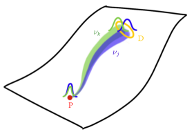
Figure 18: Decoherence in curved spacetime: drawing of neutrino wave-packet propagation from a production point P to a ”detection” point D in presence of strong gravitational fields. The widths correspond to the trajectories distributions due to the finite wave-packet width. Each wave-packet associated with a mass eigenstate follows a trajectory close to null geodesics. (Figure from Chatelain and Volpe [145].)

In core-collapse supernovae the role of trajectory bending and energy redshift was studied by few authors. For example, Fuller and Qian [235] argued that the difference in the gravitational redshift between $\bar{\nu}_{\_}e$ and $\nu_{\_}e$ can increase the electron fraction and impact $r$-process nucleosysnthesis above the nascent proto-neutron star. Yang and Kneller [522] found that trajectory bending nearby a very compact source in a supernovae produces a neutrino ”halo” similar to the one identified by Cherry et al. [148] due to $\nu\nu$ interactions. Caballero et al. [123] provided the full nucleosynthetic outcomes of $r$-process elements in black hole accretion disks models. Their results clearly show the importance of the inclusion of trajectory bending and neutrino energy redshift when determining element abundances.

Decoherence is also an important aspect of neutrino flavor evolution. Indeed, in a wave-packet description of neutrino propagation the wave-packets associated with neutrino mass eigenstates can decohere suppressing flavor oscillations (see for example [249]. In vacuum one quantifies decoherence by wave-packet separation through the ”coherence length”, $L_{\_}{\rm coh}\simeq(4\sqrt{2}E^{2}/|\Delta m^{2}|)\sigma_{\_}x$ for Gaussian wave-packets, with $\sigma_{\_}x$ the intrinsic wave-packet dispersion. Note that the Daya-Bay experiment investigated the effects of a wave-packet description of vacuum oscillations and set the first limit on its width, finding it not to be significant [47].

For supernova neutrinos, since neutrinos travel over large distances, decoherence effects by wave-packet separation can be sizable as discussed e.g. in Kersten and Smirnov [302]. Akhmedov et al. [37] investigated such effects in the density matrix formalism and showed that, in vacuum, they induce a damping of the off-diagonal terms. Moreover they studied decoherence effects in presence of dense matter and neutrino backgrounds for the cases of adiabatic and non-adiabatic evolution.

Extending the formalism to curved-spacetime, Chatelain and Volpe [143] investigated the impact of wave-packet decoherence in a Schwarzschild metric (Fig. 18). They pointed out that, in curved space-time, instead of the coherence length a coherence proper time $\tau_{\_}{coh}$ should be used to quantify decoherence. This is defined as the time at which the difference between the proper times at a ”detection” point D satisfies $\tau=\sigma_{\_}t\sqrt{B(r_{\_}D)}$. Neglecting matter and $\nu\nu$ interactions, decoherence was found to produce modifications of the proper time by several tens of a percent.

III.8 Connections: from atomic nuclei to quantum devices

Several authors have unravelled exciting connections between a weakly interacting neutrino gas and other many body systems [406, 504, 491, 366], or investigated the role of many-body correlations and of entanglement [92, 93, 91, 230, 229, 405, 105, 316, 132, 401, 432, 433, 434, 352, 44, 351]. Besides being interesting from the theoretical point of view, these studies brought novel ways to approach the problem of neutrino propagation in dense environments and opened new numerical treatments, in particular using quantum devices.

Let us first emphasize that the algebraic formulation of the neutrino Hamiltonian in dense environments allowed to establish an interesting connection between dense neutrino gases and condensed matter. Indeed, following Balantekin and Pehlivan [71], Pehlivan et al. [406] considered the Hamiltonian in Eq.(60) with the single-angle approximation

$$H =\sum_{\_}{\omega}\omega{\rm{\bf B}}_{\_}{\rm vac}\cdot{\bf J}_{\_}{\omega}+\mu\sum_{\_}{{\bf p},{\bf q}}{\bf J}_{\_}{\bf p}\cdot{\bf J}_{\_}{\bf q}\ .$$ (90)

The authors showed that the neutrino Hamiltonian Eq. (90) (without matter and for constant $\mu$) is formally equivalent to the reduced Bardeen-Cooper-Schrieffer (BCS) Hamiltonian in the theory of superconductivity [82]

$$H_{\_}{\rm BCS}=\sum_{\_}k\epsilon_{\_}kt_{\_}k^{z}+GT^{+}T^{-}\ ,$$ (91)

which describe Cooper pairs of of valence electrons in a lattice. The first term depends on the single-particle energies $\epsilon_{\_}k$ of the Cooper pairs that electrons with spin-up ($\uparrow$) or spin-down ($\downarrow$) can occupy. The second term depends on the constant $G$, representing the pairing interaction strength, and on the quasi-spin operators

$$t_{\_}k^{z}=(c^{\dagger}_{\_}{k,\downarrow}c_{\_}{k,\downarrow}-c^{\dagger}_{\_}{k,\uparrow}c_{\_}{k,\uparrow}-1)\ ,$$ (92)

and

$$T^{+}=\sum_{\_}{k}t_{\_}k^{+} =\sum_{\_}kc^{\dagger}_{\_}{k,\downarrow}c^{\dagger}_{\_}{k,\uparrow}~{}~{}~{}~{}T^{-}=\sum_{\_}kt_{\_}k^{-}=\sum_{\_}kc_{\_}{k,\uparrow}c_{\_}{k,\downarrow}\ ,$$ (93)

that obey SU(2) commutation relations. This result highlighted that the neutrino Hamiltonian is exactly solvable since, as pointed out by Richardson [428], the BCS Hamiltonian has analytical solutions thanks to the algebraic Bethe ansatz method; whereas Gaudin [243] showed the exact solvability of the model because of the number of quantum invariants. The work of Pehlivan et al. [406] was further elaborated in Pehlivan et al. [405] that included neutrino magnetic moments coupled to magnetic fields. Moreover, Fiorillo and Raffelt [215] discussed that pendulum-like solutions, identified in the context of both slow and fast modes, are analogous to soliton solutions in the BCS case.

More connections between neutrino gases in dense systems and other domains have been uncovered. Volpe et al. [504] established a formal connection between neutrinos propagating in dense media and atomic nuclei, or metallic clusters, through the BBGKY hierarchy. Moreover the authors pointed out that extended mean-field equations include the pairing correlators Eq. (61) that are formally analogous to pairing correlations in the BCS theory for superconductivity in condensed matter, or to pairing in atomic nuclei.

An analogy with fluids was pointed out by Mirizzi et al. [366] in a two-dimensional model of supernova neutrinos. The authors discussed that the instability produced by $\nu\nu$ interactions, breaking the spatial symmetry, has a nice analogy with nonlinear fluid instability. In particular, the transition from a coherent to an incoherent regime in flavor behaves like a streaming flow that changes from the laminar to the turbulent regime (Fig. 19).

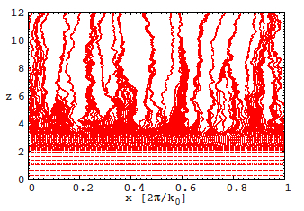
Figure 19: Analogy between non-linear fluids and supernova neutrinos with $\nu\nu$ interactions: as the translation symmetry is broken in a two-dimensional model, the streamlines of the $\nu_{\_}e$ flux along the vertical direction become irregular, showing large variations and converging towards preferred directions. This behavior is analogous to the transition from laminar to turbulent regime. (Figure adapted from [366]).

One of the crucial open questions is how many-body correlations evolve as a function of the number of particles $N$, since the Hilbert space of the corresponding wave-function increases exponentially with $N$. Developments based on the Bethe ansatz have brought the first comparisons of mean-field and exact results (for a small number of particles), showing in some cases significant differences. Cervia et al. [132], Patwardhan et al. [401] have employed concepts from quantum information theory, in particular entanglement entropy, to quantify the entanglement between neutrino states.

The entanglement entropy of a neutrino with frequency $\omega$ with the rest of the neutrinos is defined as

$$S({\omega})=-{\rm Tr}[{\varrho^{(red)}_{\_}{\omega}}{\rm log}\varrho^{(red)}_{\_}{\omega}]=-\sum_{\_}{s={\pm}}\lambda_{\_}{s,\omega}{\rm log}(\lambda_{\_}{s,\omega})\ ,$$ (94)

with the reduced density matrix obtained by tracing over all other neutrinos

$$\varrho^{(red)}_{\_}{\omega}={\rm Tr}_{\_}{(\omega^{\prime}\neq\omega)}\varrho\ ,$$ (95)

and the eigenvalues given by

$$\lambda_{\_}{\pm,\omega}={1\over 2}(1\pm|{\bf P}_{\_}{\omega}|)\ ,$$ (96)

with ${\bf P}_{\_}{\omega}$ the polarization vector (see Appendix A).

If the neutrino mode is maximally entangled with its environment, then $|{\bf P}_{\_}{\omega}|=0$, and the entanglement entropy $S({\omega})=\log(2)$. In the mean-field approximation, the many-body wave-function is the factorized product of single-particle wave-functions, giving $|{\bf P}_{\_}{\omega}|=1$ and $S({\omega})=0$. Thus the entanglement entropy gives information on the deviations from the mean-field approximation due to many-body correlations. Figure 20 shows the entanglement entropy for a system of the order of $10$ particles. The results show that the entropy is the highest for the neutrinos whose energies are the closest to the spectral split (see Figure 13 and section II.G.1).

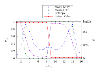
Figure 20: Probability that each neutrino is found in the $\nu_{\_}1$ state, $P_{\_}{\nu_{\_}1}$ when $\mu\leq\omega_{\_}{0}$ (the latter being the vacuum oscillation frequency) for a number of neutrinos $N=16$. Shown are the initial configurations (a $\nu_{\_}e$ at $\omega_{\_}i$ with $i=1,8$ and $\nu_{\_}x$ at $\omega_{\_}i$ with $i=8,16$). The many-body results (purple) are compared with the mean-field ones (green). The entanglement entropy $S$, that encodes information on the deviation from the mean-field results of the full many-body ones, peaks at the spectral split frequencies $\omega/\omega_{\_}{0}=3$ and 14, showing that correlations are important around the spectral-split frequencies. (Figure adapted from [401]).

After extending the Hamiltonian (90) to $3\nu$ flavors using the SU(3) algebra, Siwach et al. [463] realised the first study of the entanglement of a many-body system with $N=5$. The results show that the role of correlations increases with $N$ and can reach the maximum entanglement entropy $S({\omega})=log(3)$ (instead of $log(2)$ for 2$\nu$ flavors), as found in Patwardhan et al. [401].

Furthermore advanced numerical techniques such as tensor network methods allow to treat the time-evolution of the neutrino many-body problem for a number of particles larger than conventional methods. Cervia et al. [133] showed that, depending on the initial conditions and the number of spectral splits, some speed up can be obtained (for $N$ up to 20-25), compared to direct numerical integration methods, if one uses a time-dependent variational principle on a tensor network.

Roggero [432, 433] and Roggero et al. [434], Martin et al. [352] performed further investigations of the entanglement entropy for neutrino systems, following the real-time dynamics of systems of larger size, up to $10^{2}$ and $10^{3}$ particles.

New developments also concern numerical methods that are at variance with forward integration techniques. An example are the recent efforts to employ an inference procedure, as in the statistical data assimilation explored by Armstrong et al. [59], Rrapaj et al. [436], Armstrong [57], that look for the optimization of a cost function. The method does not require knowledge of the initial conditions, but rather constraints at some locations of the coordinate axis (not necessarily at the bounds) that parametrize the model equations of motion.

Finally, recent studies are opening the exciting possibility to investigate correlations and entanglement of strongly correlated neutrinos on quantum computers. Hall et al. [265] studied the evolution, the entanglement entropy (of a pair) and concurrence of a 4 particle neutrino system using, for the first time, a quantum device. Amitrano et al. [44] considered trapped-ion qubits.

The results obtained so far for (very) small $N$ are exploratory and indicate the potential impact of many-body correlations in this context. However, it is important to keep in mind that to definitely assess the role of many-body correlations and the reliability of the mean-field approximation, we will need to go to very large number of neutrinos. This is computationally very challenging. Having highlighted aspects of our understanding of neutrino flavor evolution in dense environments, we now turn to observations.

IV Past and future observations

IV.1 SN1987A

On the 23^rd of February 1987 Sk-69^∘202 exploded in the Large Magellanic Cloud, a satellite galaxy of the Milky Way, producing SN1987A [60, 98, 423]. It was the first naked-eye since Kepler’s supernova (Ia) in 1604. Measurements based on the expanding photosphere method agreed within 10 $\%$ [452] that the supernova was located at 50 $\pm$ 5 kpc from the Earth. Nowadays the distance to the LMC is known within 1$\%$, i.e. $49.59\pm 0.09~{}(stat)\pm 0.54~{}(sys)$ kpc, based on eclipsing binary systems [409].

SN1987A was unique in many respects. Its progenitor, the first known, was a blue supergiant, whereas supernovae progenitors were thought to be red supergiants. This became the blue problem [60, 98] (for a recent discussion e.g., see [517]). The earlier SN1054, seen by Chinese astronomers, left a pulsar in the Crab nebula. It has taken slightly more than thirty years to finally have indications for a compact object, likely a neutron star, at its location [42, 153, 394]. The inner ring, large mixing and asymmetrical ejecta of SN1987A indicated strong asphericity in the explosion (see Arnett et al. [60], Podsiadlowski [411], Janka [290] and Figure 1).

SN1987A, the closest supernova in the last hundreds of years, was observed in all wavelengths from gamma rays to radio, and for the first time, neutrinos from the collapse of the stellar core were detected. Suzuki [474], at its 20th anniversary, gave a lively description of this pioneering observation. The water Çerenkov detector KII [278] observed a neutrino burst of 11 events of energy 7.5 to 36 MeV in 13 s; while IMB [104] measured 8 events in 6 s with 20 MeV to 40 MeV. BST [41] detected a burst of 5 events in 9 s and, about 5 h before, the Mont Blanc Liquid Scintillator Detector (LSD) [24] recorded 5 events during 7 s with energy $\geq$ 7 MeV (Fig. 21). Since no signal has been found correspondingly in the other detectors, the LSD events remain controversial.

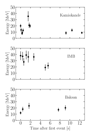
Figure 21: Neutrino events from SN1987A at Kamiokande, IMB and Baksan: energies correspond to secondary positrons produced in inverse $\beta$-decay. Events have been shifted at same t=0 (clock relative offsets are unknown). (Figure from Fiorillo et al. [217].)

Assuming energy equipartition among the neutrino species, early analysis [445, 455, 60] and subsequent studies based on two-dimensional likelihoods [327, 396, 493, 78, 213] showed the total energy associated with the neutrino events from SN987A to be $5\times 10^{-52}~{}$erg at best-fit value, confirming Colgate and White’s hypothesis, and that the spectra agree reasonably well with thermal expectations with $\bar{\nu}_{\_}e$ temperatures $T=4$ MeV (best fit). Analysis of the neutrino time signal agreed with the expected supernova pulse duration of about 10 s and exponential neutron star cooling. Therefore, SN1987A events confirmed the global picture of the neutrino emission during a gravitational core-collapse supernova explosion.

Moreover, the Bayesian analysis of the time signal by Loredo and Lamb [327] and by Pagliaroli et al. [396] supported the delayed-shock over the favored prompt-shock model by unambiguously showing the presence of an accretion phase. From nuclear matter equations of state, the formation of a neutron star (instead of a black hole was favored, with mass [445] and radius [327, 396] compatible with expectations. The radius of the neutrino emitting surface was found to be 18 km [423].

The observation of neutrinos from SN1987A was confirming suggestions and results obtained by the supernova modelers. It was Baade [67] who first suggested that in supernovae the tremendous energy comes from the gravitational collapse of the inner core into a neutron star. Hoyle and Fowler [287] proposed stars could dye due to thermonuclear runaway (SN Ia) of degenerate material or implosion of the stellar core (SN II and Ib/c). Colgate and Johnson [156] pointed out that the collapse could be followed by core bounce and shock formation. The shock would expel most of the star’s mass by propagating into the mantle.

To support the prompt-shock model, Colgate and White [157] hypothesized that most of the gravitational binding energy of the imploding core, $E_{\_}b\sim GM_{\_}{\rm NS}^{2}/R_{\_}{\rm NS}$, ($M_{\_}{\rm NS}$ and $R_{\_}{\rm NS}$ being the mass and radius of the newly formed neutron star) namely $[1.5,4.5]\times 10^{-53}~{}$erg, would be emitted with neutrinos. A few percent of the energy deposited by neutrinos back into matter energy, could drive the supernova explosion. In the early seventies, Freedman [226] suggested that neutrinos could scatter coherently on nuclei with a large cross section at neutrino energies below 100 MeV. He pointed out that this coherent effect might impact $\nu$ emission during stellar collapse and neutron star cooling. This gave a new insight on the role of $\nu$ in dense astrophysical ennvironments. Later on, Bethe and Wilson [100] shaped the model for supernova explosions into the delayed neutrino-heating mechanism.

The information on the about 24 neutrinos from SN1987A has been a marvelous laboratory for particle physics and astrophysics. The neutrino signal gave the start of the explosion, the energy released in the gravitational collapse, the temperature at the neutrinosphere, information on the explosion mechanism on the one hand, e.g. rejecting the favored prompt bounce-shock model and supporting the delayed neutrino-heating mechanism, and giving limits on neutrino properties and non-standard physics on the other.

But, is the delayed neutrino-heating mechanism that drives the explosion of most core-collapse supernovae? Early one-dimensional calculations faced shock stagnation. SN1987A observations of asymmetries and the presence of strong hydrodynamic mixing processes, during the explosion, gave momentum to the development of multi-dimensional simulations. With the advent of two-dimensional simulations, investigations showed the region behind the shock to be convectively unstable, then the shock itself to be unstable to radial perturbations (the SASI) and finally that, neutrino-driven convection being turbulent, turbulence could aid the shock propagate at larger radii (see, e.g. Mezzacappa [360] and references therein).

Thanks to this impressive progress in ascertaining the explosion mechanism, since few years a consensus has been emerging across the supernova community. Indeed simulations show that the majority of supernovae explodes because of the delayed neutrino-heating mechanism, where neutrinos efficiently reheat the shock aided by convection, turbulence and the SASI [360]. However there is for example not yet a consensus on the role of the SASI for all progenitors (see, e.g.Burrows et al. [121, 122]). More generally, different groups might not obtain similar outcomes for the same progenitor because of differences in numerical treatments, e.g. of the neutrino transport, or on the progenitor. Rotation and magnetic fields can also help explosions, and their effects are being studied (see for example Kotake et al. [311], Kuroda et al. [315]). Notwithstanding, the answer to this longstanding unresolved question appears to be close.

Analyses of the SN1987A events have produced a wealth of information on non-standard neutrino properties, interactions or particles [423, 533]. For example, neutrinos flew through space for 1.6 $\times 10^{5}$ years, yielding a bound on the neutrino lifetime of $\tau/m>5\times 10^{5}$ s/eV [278, 98]. The non-observation of a $\gamma$-ray signal over background, in correspondence with the neutrino time signal, gave stringent bounds on the neutrino lifetime from radiative decays [423, 253, 533]. Optical brightening followed neutrino emission by a few hours. Neutrino propagation through space, at nearly the same speed as photons, gave a tight constraint on the neutrino speed $c_{\_}{\nu}$, i.e. $|(c-c_{\_}{\nu})/c|<2\times 10^{-9}$ [326]. Moreover, the absence of a dispersion of the neutrino pulse gave upper limits on the neutrino charge and on the $\nu_{\_}e$ mass (about 20 eV, now excluded).

As for neutrino non-radiative two-body decay, Figure 22) shows a comparison of the sensitivity of experiments using different neutrino sources on to $\tau/m$, the lifetime-to-mass ratio. One can see that neutrinos from core-collapse supernovae and the DSNB have a unique sensitivity window. As for SN1987A, Iváñez Ballesteros and Volpe [78] performed a full 3$\nu$ flavor study of neutrino non-radiative two-body decay. Using spectral information of the neutrino events, the authors derived the bound $\tau/m\geq 2.4~{}(1.2)\times 10^{5}$ s/eV at 68 (90) $\%$ CL for $\nu_{\_}2$ and $\nu_{\_}1$ (inverted mass ordering), competitive to cosmological bounds.

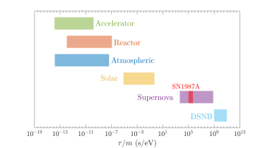
Figure 22: Neutrino two-body non-radiative decay: the figure shows the sensitivity to the lifetime-to-mass ratio for experiments exploiting different neutrino sources. The bands are obtained by assuming an exponential depletion of the initial neutrino flux, with only $1\%$ or $99\%$ of it reaching the detectors. The red band for SN1987A assumes a distance of 50 kpc. Typical neutrino energies and distances are assumed for the other neutrino sources.(Figure from Iváñez Ballesteros and Volpe [78].)

Furthermore, energy-loss arguments on the shortening of SN1987A $\nu$ time signal, associated with the neutron star cooling, gave limits on the neutrino magnetic moment [81], on right-handed neutrinos or currents, on axions and axion-like particles (see e.g. [141, 404]), on dark photons (see e.g. [341] . Considering Majoron-like bosons decaying to neutrinos, the absence of a SN1987A flux with $E>$100 MeV provides a strong bound on neutrino Majoron-coupling for Majorons with 100 eV $<m_{\_}{\phi}<100$ MeV [217].

The impact of flavor mechanisms on SN1987A $\nu$ data was also investigated. Jegerlehner et al. [292] studied the sensitivity of SN1987A events to the MSW effect. It is to be noted that in this early analysis the priors for $\langle E_{\_}{\bar{\nu}_{\_}e}\rangle$ and $\langle E_{\_}{\bar{\nu}_{\_}{\mu,\tau}}\rangle$ were based on supernova simulations with incomplete microphysics, which was yielding too large $\langle E_{\_}{\bar{\nu}_{\_}{\mu,\tau}}\rangle$, i.e. in the range [24, 27] MeV. In their analysis including MSW, the authors found that hot $\bar{\nu}_{\_}e$ spectra were marginally compatible with observations, correctly pointing to an inconsistency.

Lunardini and Smirnov [337] performed a model-dependent analysis of the spectral modifications of SN1987A events, due to the MSW effect, and found it to be significant. However, the likelihood analysis by Vissani [493] based on modern supernova fluxes showed the impact of the MSW phenomenon to be small and comparable to effects from other inputs (e.g. backgrounds, detector thresholds, …). Furthermore, with a similar analysis, Iváñez Ballesteros and Volpe [78] showed that the best fit and confidence contours of the $\bar{\nu}_{\_}e$ average energy and luminosity also depend on the pinching parameter, producing variations are at the same level as other inputs. Finally the analysis of the time and energy of the SN1987A neutrino events by Dedin Neto et al. [179] agreed on a preference for the accretion model, as in previous findings, and showed a slight preference for the MSW mechanism (normal mass ordering).

Besides the studies on the impact of flavor phenomena, detailed comparisons are being realized between SN1987A data and supernova simulations. Olsen and Qian [390] compared one-dimensional supernova models to K-II data based on Bayesian analysis. On the other hand, Li et al. [323] confronted outcomes of multi-dimensional supernova models with SN1987A data during the first second, finding disagreement even when considering different flavor scenarios (MSW effect, flavor equilibration due to the $\nu\nu$ interaction). On the contrary Fiorillo et al. [213] did a detailed comparison of one-dimensional supernova simulations with the SN1987A observations finding an agreement with the early neutrino signal. The late neutrino time signal appears to be too short, which might point to the role of convection in the proto-neutron star. Clearly, further progress towards obtaining consistent three-dimensional successful supernova models will shed more light on the consistency between modern simulations and the neutrino events from SN1987A.

The ensemble of the results extracted so far from SN1987A observations is emblematic of how much patience for such rare events can be rewarded in scientific knowledge and progress.

IV.2 From the next supernova

If a supernova explodes in the future, neutrinos emitted in the first instants of the core-collapse will be detected several hours before optical emission, and will guide optical instruments [18]. If the supernova is nearby, pre-supernova neutrinos from thermal [388] and weak processes [400] in the late stages of the stellar evolution could be observed preceding core-collapse and give advanced warning [524] as well as information on the supernova progenitor (see the review by Kato et al. [299]). SK could detect about 200 pre-supernova neutrinos 12 hours before collapse of a 15-25 ${\rm~{}M}_{\_}{\odot}$ star at 0.2 kpc (such as Betelgeuse); whereas SK-Gd and KamLAND could reach 0.6 kpc [18] and 0.69 kpc [62] respectively. Moreover, if close enough, one could measure the neutrino lightcurve up to 100 s, as first pointed out by Li et al. [324], which would yield interesting information on the late cooling phases of the newly formed proto-neutron star.

The observation of the next supernova will benefit of the SNEWS network [40] and of dark matter detectors (see e.g. [25, 318]. From the complementarity of the technologies available, we shall measure the time and energy of neutrino flavors through inverse $\beta$-decay, neutrino-nucleus scattering, neutral current scattering on electrons as well as on protons [88], and coherent neutrino-nucleus scattering [39].

For inverse $\beta$-decay the cross sections are precisely known [467, 427]. On the contrary, the cross sections associated with charged-current $\nu$-nucleus interactions, in particular on ¹⁶O, ⁴⁰Ar, ⁵⁶Fe, ²⁰⁸Pb are still affected by theoretical uncertainties, that can reach several tens of a percent (Cfr. for example Fig. 5 of Väänänen and Volpe [490] for the lead case). The two exceptions include deuterium whose cross sections are known with a few percent precision [75], and ¹²C [503, 276].

Volpe [499, 501] suggested to use a novel technique, i.e. the low energy beta-beam, also to perform $\nu$-nucleus cross section measurements at energies of interest for supernovae. More than twenty years after the proposal at the Spallation Neutron Source [66, 80], neutrinos from decay-at-rest muons are being used for such experiments. The results of the first two measurements on the inclusive $\nu_{\_}e$ charged-current cross section on ¹²⁷I [49] and $\nu_{\_}e$ on ^natPb [48] have been released. More nuclear targets will be studied, including ⁴⁰Ar, important for the DUNE experiment.

Besides providing a better knowledge of the spin and spin-isospin weak nuclear response to neutrinos, in the energy range of interest for the detection of supernova neutrinos, such measurements could shed further light on the issue of the quenching of the axial-vector coupling constant, also for forbidden states, as pointed out by Volpe [500]. Recently, using effective field theories and powerful quantum many-body techniques, Gysbers et al. [263] have shown that the quenching of the allowed Gamow-Teller transitions arises from strong correlations in the nucleus and weak interaction coupling to two nucleons. Indeed this result represents a major step forward, since this quenching, observed in beta-decay and in charge-exchange reactions, has been an open controversial issue for 50 years.

The future observation of a supernova time signal will be rich of fundamental lessons. As supernova simulations show, according to the current paradigm, the neutrino time signal involves three main characteristic phases: the neutronization burst, the accretion phase and the cooling of the newly born proton-neutron star. An example is Figure 23 which provides the outcome of a self-consistent three-dimensional simulation by Bollig et al. [111] that reaches an explosion energy (at infinity) of 1 Bethe (10⁵¹ erg) and a ⁵⁶Ni amount of $\leq 0.087{\rm~{}M}_{\_}{\odot}$ in agreement with SN1987A observations (wthin 10$\%$).

During the first tens of ms, $\nu_{\_}e$ are emitted due to the capture of the electrons by the nuclei, that, with iron photodissociation, contribute to the core collapse. These neutrinos form the so-called neutronization peak. Then the neutrino emission is powered by the accretion flow (accretion phase) during which all neutrino flavors are produced. The signal presents fast variations and directional dependence due to large convection and hydrodynamic instabilities and the LESA. Finally, when the explosion is ongoing, and shock stagnation overcome, neutrinos are emitted from the cooling of the proton-neutron star and the luminosity drops. From Figure 23 one can see how much the hierarchy of average energies $\langle E_{\_}{\nu_{\_}e}\rangle<\langle E_{\_}{\bar{\nu}_{\_}e}\rangle<\langle E_{\_}{\nu_{\_}x}\rangle$ is satisfied.

The $\nu_{\_}e$ flux from the 50 ms neutronization-burst represent less than 1$\%$ of the total neutrino luminosity. The accretion phase that lasts from few tens to few hundreds ms and the neutron star cooling about 10 seconds take away most of the gravitational binding energy. Each of these phases has its own specificities from the point of view of the supernova evolution and of neutrino flavor conversion as we will discuss.

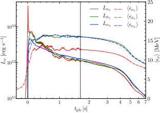
Figure 23: Neutrino supernova time signal: the figure presents the luminosities $L_{\_}{\nu}$ and the average energies $\langle\epsilon_{\_}{\nu}\rangle$ of $\nu_{\_}e$, $\bar{\nu}_{\_}e$ and of $\nu_{\_}x$ (the latter stand for $\nu_{\_}{\mu},\bar{\nu}_{\_}{\mu},\nu_{\_}{\tau},\bar{\nu}_{\_}{\tau}$). The results correspond to the three-dimensional simulation of a nearly 19 ${\rm~{}M}_{\_}{\odot}$ progenitor followed from about 7 minutes before the onset of explosion up to 7 seconds. There are three characteristic phases: the $\nu_{\_}e$ neutronization peak (about 20 ms), the $\nu_{\_}e$, $\bar{\nu}_{\_}e$ and $\nu_{\_}x$ ($\bar{\nu}_{\_}x$) emitted during the accretion phase (about 500 ms) and the cooling of the newborn neutron star. (Figure from Bollig et al. [111].)

If the supernova is close enough, the precise measurement of the time signal will be crucial to definitely assess the explosion mechanism through the identification of oscillations with high frequencies, correlated with SASI, whose measurement requires a very precise time resolution, as the one e.g. in the IceCube detector (see for example [505, 480, 372]). In this respect, modifications from flavor evolution should not swamp the signature.

The measurement of early ($<20$ ms) stages of neutrino emission would give information on the bounce time [267]. Note that this is key to estimate the burst time of the gravitational waves [395] which are mainly produced by the oscillations of the newly formed proto-neutron star [16]. The concomitant multimessenger event of neutrino and gravitational waves from a core-collapse supernova was discussed also for example by Halim et al. [264].

From the point of view of flavor evolution, the neutronization-burst represents a unique phase. Only the MSW effect appears to influence the neutrino spectra. Neither fast nor slow modes are at work, as we understand them now. The former requires crossings in the neutrinos and antineutrinos angular distributions, the latter $\nu\bar{\nu}$ pairs (in the bulb model). Moreover there are neither effects from shock waves, since shock waves reach the MSW region after 1-2 s, nor from turbulence. Therefore, the neutronization-burst appears to be a good laboratory to explore non-standard properties. These include for example non-standard $\nu\nu$ interactions [164] or neutrino non-radiative decay [52, 177].

Since flavor mechanisms produce neutrino spectral modifications (see Section II.B), an important question to ask is with which precision we will be able to reconstruct the supernova neutrino fluxes when the next supernova blows off (see for example [490, 330, 331, 239]). The answer obviously depends on which observatories will be operating at that time and on the supernova distance.

It is interesting to note that a precise determination and reconstruction of the supernova neutrino spectra might not be trivial in likelihood analysis where the ensemble of the parameters are left free to vary, even in the simplest case with the MSW effect. Indeed Minakata et al. [364] pointed out the presence of parameter degeneracies that can in principle be broken by combining detection channels [240]. However, while most of the neutrino parameters appear to be precisely measurable (for a supernova at 10 kpc) identifying the neutrino pinching for some of the flavors might be more tricky [241].

As for unknown neutrino properties, the neutrino signal from the next supernova could be a good laboratory to determine the neutrino mass ordering for which there are currently hints with a low statistical significance. The passage of the shock wave can be pictured as it goes through the MSW region (see section II.D). Shock waves effects can be important and produce distortions of the positron (or electron) time signals, depending on the neutrino energy and mass ordering (see for example [476, 218, 336, 222, 307] and the reviews by Duan and Kneller [192], Horiuchi and Kneller [284]). Also, the rise time of the neutronization-burst can be used to determine the neutrino mass ordering in a detector like IceCube [456]. Although these signatures are interesting, it is likely that Earth-based experiments like JUNO, DUNE or Hyper-K will measure the neutrino mass ordering before the next supernova blows off. In particular it should be measured at about 3 $\sigma$ after 6 [45] or 10 years [17] respectively.

As for CP violation in the lepton sector, hints for $\sin\delta<0$ (90 $\%$ CL) indicates that the CP violating phase should be discovered soon from the DUNE and Hyper-K experiments. The effects of the Dirac CP violating phase was studied in the context of core-collapse supernovae. Akhmedov et al. [38] concluded that there should be no impact of the Dirac phase on the $\nu_{\_}e$ fluxes in a supernova, even if the $\nu_{\_}{\mu}$ and $\nu_{\_}{\tau}$ fluxes are unequal. In contrast with such findings Balantekin et al. [74] demonstrated that the Dirac phase can impact the electron neutrino fluxes if the muon and tau neutrino fluxes differ, because of e.g. radiative corrections or of non-standard interactions, such as flavor-changing neutral currents. The result relies on a factorization condition of the neutrino Hamiltonian, i.e. ${\cal H}(\delta)=S^{\dagger}{\cal H}(\delta=0)S$ with $S^{\dagger}(\delta)={\rm diag}(1,1,e^{i\delta})$. Physics that breaks such condition can engender CP violation effects on the $\nu_{\_}e$ fluxes.

These findings were generalized in presence of $\nu\nu$ interactions by Gava and Volpe [245], beyond the mean-field to the full many-body problem [405] and on the neutrino degeneracy parameter in the early universe [246]. In the supernova numerical calculations showed the impact of the phase to be small [74]. However, the combined effect of the Majorana CP violating phase(s) and the neutrino magnetic moment could trigger sizable effects, opening the possibility for new resonances, as pointed out by Popov and Studenikin [414].

Obviously, even when the mass ordering and CP violation will be precisely measured, supernova neutrinos will remain interesting probes for non-standard physics. Indeed there are numerous flavor mechanisms related to other key unknown neutrino properties that have been extensively discussed in the literature, such as sterile neutrinos, non-standard interactions, or the neutrino magnetic moment (see for example which can give sizable modification of the neutrino spectra in presence of strong magnetic fields, in core-collapse supernovae or nearby compact objects Nunokawa et al. [384], Pehlivan et al. [405], Giunti and Studenikin [253], Sasaki and Takiwaki [444]).

IV.3 Towards the discovery of the diffuse supernova neutrino background

Complementary to a single supernova is the DSNB, made of neutrinos emitted by past core-collapse supernovae. The DSNB is nearly isotropic and constant in time. It depends on cosmology, astrophysics and particle physics (see the reviews by Ando and Sato [55], Beacom [87], Lunardini [334], Mathews et al. [354], Suliga [469], Ando et al. [54]).

The DSNB flux, including a progenitor dependence, reads

$$\phi_{\_}{\nu_{\_}{\alpha}}(E_{\_}{\nu})={c}\int\int{\rm dM}~{}dz~{}\Big{|}{dt_{\_}{\rm c}\over{dz}}\Big{|}~{}R_{\_}{\rm SN}(z,{\rm~{}M})~{}{\phi_{\_}{\nu_{\_}{\alpha}}(E^{\prime}_{\_}{\nu},{\rm~{}M})}\ ,$$ (97)

where $z\in[0,z_{\_}{max}]$ is the cosmological redshift, $c$ is the speed of light, $E_{\_}{\nu}^{\prime}$ is the neutrino energy at the star location at redshift $z$, related to the energy $E_{\_}{\nu}$ on Earth through $E_{\_}{\nu}^{\prime}=E_{\_}{\nu}(1+z)$, $\phi_{\_}{\nu_{\_}{\alpha}}(E_{\_}{\nu}^{\prime},M)$ is the time-integrated neutrino flux for a progenitor of mass M.

A progenitor mass dependence of the DSNB flux was first included by Lunardini and Tamborra [338]. It is to be noted that the most general expression for the DSNB flux should also have an explicit dependence on the galactic chemical evolution, as considered for example by Nakazato et al. [378], Ashida et al. [64]. In Eq. (97) usually $z\in[0,5]$. However only the lowest redshifts, i.e. $z\in[0,2]$ give the most important contribution to the DSNB flux. Moreover note that the integral on the progenitor mass covers the range ${\rm M}\in[8,125]{\rm~{}M}_{\_}{\odot}$ (taking $100{\rm~{}M}_{\_}{\odot}$ does not introduce any significant difference).

The first factor in Eq.(97) is the cosmological time that depends on the cosmological model. Usually the $\Lambda$CDM model is assumed. The expansion history of the universe is then

$$\Big{|}{dz\over{dt_{\_}{\rm c}}}\Big{|}=H_{\_}0(1+z)\sqrt{\Omega_{\_}{\Lambda}+(1+z)^{3}\Omega_{\_}m}\ ,$$ (98)

with $\Omega_{\_}m$ and $\Omega_{\_}{\Lambda}$ the matter and the dark energy cosmic energy densities, $H_{\_}0=70~{}$km s^-1 Mpc^-1 is the Hubble constant. DSNB predictions show that the DSNB is not sensitive to variations compatible with the Hubble tension.

The second important input in Eq.(97) is the evolving core-collapse supernova rate $R_{\_}{\rm SN}(z,{\rm~{}M})$ that is related to the star-formation rate history $\dot{\rho}_{\_}*(z)$ according to

$$R_{\_}{\rm SN}(z,{\rm M})=\dot{\rho}_{\_}*(z){\phi({\rm M})d{\rm M}\over{\int^{125{\rm~{}M}_{\_}{\odot}}_{\_}{0.5{\rm~{}M}_{\_}{\odot}}\phi({\rm M}){\rm M}d{\rm M}}}\ ,$$ (99)

where $\phi(\rm M)$ is the initial mass function.

With his seminal work Salpeter [440] introduced the power law initial mass function

$$\phi(\rm M)\sim{\rm M}^{\chi}\ ,$$ (100)

for ${\rm M}\in[0.5,1]~{}{\rm M}_{\_}{\odot}$. The quantity $\phi(\rm M)d(\rm M)$ gives the number of stars in the mass interval $[\rm M,\rm M+d\rm M]$. Since, the Salpeter IMF has been employed, $\chi$ being determined with an uncertainty of about $10\%$. Baldry and Glazebrook [77] introduced a modified broken power law for the IMF with $\chi=-1.5$ at $0.1~{}{\rm M}_{\_}{\odot}\leq{\rm M}\leq 0.5~{}{\rm M}_{\_}{\odot}$ and $\chi=-2.12$ for ${\rm M}>0.5~{}{\rm M}_{\_}{\odot}$. Note that such a modified IMF gives a similar result for $R_{\_}{\rm SN}(z,{\rm M})$ [281]. The universality of the IMF at high masses, i.e. the fact that it is the same in all environments and throughout cosmic time, is being discussed (see for example by Ziegler et al. [532]).

As for the cosmic star-formation history, it can be deduced from observations (see e.g. [280, 425, 438]) and described by a piecewise continuous form of a broken power law by Yüksel et al. [526] (see also [340, 462])

$$\dot{\rho}_{\_}*(z)=\dot{\rho}_{\_}{0}\Big{[}(1+z)^{\alpha\eta}+\Big{(}{1+z\over{B}}\Big{)}^{\beta\eta}+\Big{(}{1+z\over{C}}\Big{)}^{\gamma\eta}\Big{]}^{-1/\eta}\ ,$$ (101)

with $\alpha=3.4,\beta=-0.3,\gamma=-3.5$ the logarithmic slopes at low, intermediate and high redshift. The quantity $\eta=-10$ is the smoothing function and the constants defining the redshift breaks are $B=5000$, $C=9$. In the cosmological model considered by Yüksel et al. [526], $\Omega_{\_}m=0.3$ and $\Omega_{\_}{\Lambda}=0.7$ and $H_{\_}0=70~{}$km s^-1 Mpc^-1.

Concerning the cosmic star-formation rate history, several parametrization are available in the literature. The one given by equation (101) from Yüksel et al. [526], Horiuchi et al. [281] includes GRB data $z>4$ and is commonly employed.The parametrization in Fogli et al. [221] is outdated, whereas the one in Priya and Lunardini [415] present kinks. Mathews et al. [355] suggested an alternative parametrization by including only the subset of the star-formation rate data corrected for extinction by dust (Figure 24).

Currently, the local core-collapse supernova rate is known with the following precision

$$R_{\_}{\rm SN}(0) =\int^{125{\rm~{}M}_{\_}{\odot}}_{\_}{8{\rm~{}M}_{\_}{\odot}}R_{\_}{\rm SN}(0,{\rm M}){\rm d}{\rm M}$$

$$=(1.25\pm 0.5)\times 10^{-4}{\rm yr}^{-1}{\rm Mpc}^{-3}\ .$$ (102)

Moreover there is a disagreement by a factor 2 at $0\leq z\leq 1$ between the core-collapse supernova rate deduced from the star-formation rate history and the one from direct core-collapse supernova observations [282]. This is known as the ”supernova rate problem”. The uncertainty on the evolving core-collapse supernova rate constitutes one of the largest uncertainties in the DSNB predictions (Figure 24).

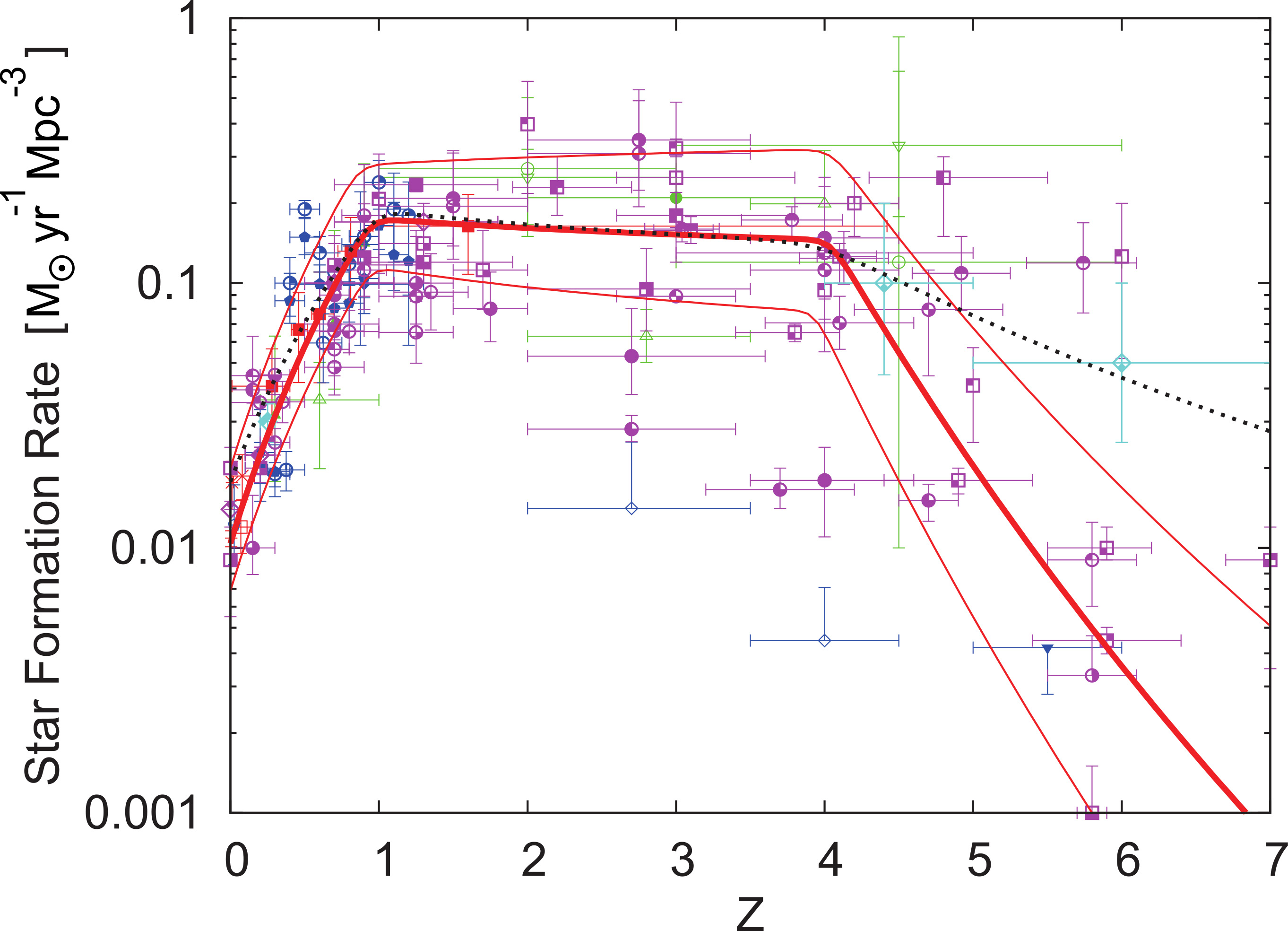
Figure 24: The figure shows a piecewise linear star formation rate fit to observed dust-corrected data. Data in IR, optical, UV, X-ray/$\gamma$-ray and radio-bands are shown by the red, blue, magenta, light-blue and green points respectively. The $\chi^{2}$ fit to the star formation rate and the $\pm 1\sigma$ upper and lower limits as a function of redshift, are shown by the red full and dotted lines respectively. The black dotted line shows the star formation rate obtained with the full data used in the work of Yüksel et al. [526]. Note that only the low $z$ part contributes to the DNSB. (Figure from [355].

The third and last important factor is the neutrino flux from one single-supernova with progenitor mass ${\rm M}$. Lunardini [333] pointed out the relic supernova background can receive a significant contribution from failed supernovae (collapsing into a black hole). Indeed, due to the compression of baryonic matter during black hole formation, the supernova generates large neutrino fluxes with higher average energies and larger differences among flavors than optical supernovae, depending on the soft or stiff equation of state, as pointed out by Sumiyoshi et al. [471].

Although the fraction of supernovae that turn into a black hole is sub-leading, this contribution influence the tail of the DSNB spectrum and contributes substantially to the DSNB rates. The dependence on the progenitor mass was first included by Lunardini and Tamborra [338] using detailed long-term supernova simulations. If one includes the neutrino spectra from core-collapse supernovae that leave a neutron star or a black hole, Eq.(97) becomes

$$\phi_{\_}{\nu_{\_}{\alpha}}(E_{\_}{\nu})= {c}\int dz~{}(1+z)\Big{|}{dt_{\_}{\rm c}\over{dz}}\Big{|}$$ (103)

$$\times\left[\int_{\_}\Omega~{}{\rm dM}~{}R_{\_}{\rm SN}(z,{\rm~{}M})~{}{\phi_{\_}{\nu_{\_}{\alpha}}^{\rm NS}(E^{\prime}_{\_}{\nu},{\rm~{}M})}\right.$$

$$+\left.\int_{\_}\Sigma~{}{\rm dM}~{}R_{\_}{\rm SN}(z,{\rm~{}M})~{}{\phi_{\_}{\nu_{\_}{\alpha}}^{\rm BH}(E^{\prime}_{\_}{\nu},{\rm~{}M})}\right]\ ,$$

where $\Omega$ and $\Sigma$ correspond to the range of masses for which the collapse gives a NS or a BH. Thus the BH fraction is given by

$$f_{\_}{\rm BH}=\frac{\int_{\_}\Sigma d\rm M\phi(\rm M)}{\int_{\_}{8\rm M_{\_}\odot}^{125\rm M_{\_}\odot}d\rm M\phi(\rm M)}.$$ (104)

Note that Schilbach et al. [450] investigated the DSNB only coming from black hole accretion disks.

The fraction of failed supernovae is currently debated. It has been argued by O’Connor and Ott [387], Horiuchi et al. [285], Ugliano et al. [488], Horiuchi et al. [286] that the star compactness could be a good indicator of the fraction of supernovae leaving black holes. This is in contrast with Ertl et al. [203] who suggested as indicators two parameters, $M_{\_}4$ and $\mu_{\_}4$, giving the enclosed mass and its derivative (s = 4, dimensionless entropy per nucleon), to better predict successful explosions in the neutrino driven wind mechanism. On the observational side, a decade long search for failed supernovae found a fraction of failed supernovae of $f_{\_}{\rm BH}=0.16+0.23-0.12$ at 90 $\%$ CL (see Neustadt et al. [382] and references therein).

Figure 25: The figure shows the current spread on DSNB $\bar{\nu}_{\_}e$ flux predictions as a function of neutrino energy. The results correspond to the predictions by Horiuchi et al. [283], Tabrizi and Horiuchi [475], Kresse et al. [312], Horiuchi and Kneller [284], Nakazato et al. [378], Galais et al. [237], Horiuchi et al. [281], Lunardini [333], Ando [51]. The labels refer to neutrino normal mass ordering (NH), inverted mass ordering (IH), neutron star (NS) and black hole (BH). (Figure from [20]).

Predictions of the DSNB flux and rates have different levels of sophistication with respect to astrophysical inputs (including black-hole fraction, contribution from binaries, evolving core-collapse supernova rate, shock waves and shock wave revival time, dense matter equation of state) on the one hand; neutrino flavor mechanisms, neutrino properties and new physics on the other. Besides the astrophysical uncertainties previously mentioned, the neutrino fluxes from one single supernova with progenitor mass M also have important variations. Figure 25 shows the current spread on the predictions of the DSNB fluxes.

Already twenty years ago, Ando and Sato [55] pointed out that the most of the DSNB flux would come from low redshifts, i.e. $0<z<1$; whereas the higher redshifts ($z>1$) would contribute at low energy ($E<$10 MeV). The authors emphasized that the early SK limit by [343] was just above predictions when employing realistic evolving core-collapse supernova rate and neutrino spectra.

Concerning the black-hole fraction, its value is treated either in a parametrized form, or obtained from extensive supernova simulations. For example in Tabrizi and Horiuchi [475], Moeller et al. [368], Ivanez-Ballesteros and Volpe [288], Priya and Lunardini [415] the progenitor mass dependence and the fraction of failed supernovae was implemented based on one-dimensional supernova simulations. It is to be noted that according to the detailed simulations by Kresse et al. [312] the BH fraction ranges from 17 $\%$ to 41 $\%$. Kresse et al. [312], Moeller et al. [368], Horiuchi et al. [286, 283] performed extensive supernova simulations (100 to 200 models) to include a detailed progenitor mass dependence. Kresse et al. [312] and Horiuchi et al. [283] also included helium-star progenitors to account for contributions from binaries, currently unknown, showing it can be significant. In their detailed study Horiuchi et al. [286] argued the compactness to be a good indicator of the fate of a supernova, as previously mentioned, and found that the DSNB detection could test small values, namely $f_{\_}{\rm BH}>20\%$.

Several authors investigated the sensitivity of the DSNB to the nuclear equation of state [368, 63, 378]. Moeller et al. [368] showed it to be statistically poor. On the other hand the authors found, with a joint analysis of Hyper-K, DUNE and JUNO events that the BH fraction can be confirmed at $90\%$ CL if it is $\geq 20\%$; and a sensitivity to the local supernova rate at 20-33 $\%$ (20 years running). Ashida and Nakazato [63] also examined the dependence of the DSNB fluxes on the equation-of-state for both its NS and BH contributions. Their results showed that Hyper-K could test the $f_{\_}{\rm BH}$-$f_{\_}{\rm HNS}$ at $3\sigma$ level in 10 years running. In a subsequent investigation, besides the dependence on the equation-of-state,Ashida et al. [64] proposed a new model for the chemical evolution of galaxies, where the IMF is varied with the galaxy type. The authors found a significant increase at low energy (extra contribution from early-type galaxies) and at higher energy (more frequent BHs) which could be discriminated from the other models considered through a Bayesian analysis of the events in SK-Gd and Hyper-K.

Some of the DSNB predictions are anchored to the SN1987A neutrino signal. First Lunardini [332] used neutrino spectral information from SN1987A and direct information on the supernova rate, finding the DSNB flux to be a factor of 4 smaller than the early upper limit by [343]. Yüksel and Beacom [525] discussed the compatibility of the spectra detected in Kam-II and IMB and showed the two were consistent. Using inferential statistical methods their DSNB predictions showed a significant flux in the detectable window ($E\in[10,18]$ MeV). Using SN1987A analysis to model neutrino emission, Vissani and Pagliaroli [494] also obtained DSNB predictions finding about 1 event/year for Super-K to 1-3 events/year, when Gd is included.

Predictions on the DSNB neutrino spectra and rates are influenced by flavor conversion mechanisms as well. The established MSW effect is routinely implemented in predictions [55, 237, 135, 415, 368, 286, 312, 288, 475, 175, 199, 63, 64]. So far only a few studies implemented flavor effects beyond the MSW mechanism.

Lunardini and Tamborra [338] and Chakraborty et al. [135] studied the influence of collective neutrino oscillations due to the $\nu\nu$ interaction which produces single or multiple spectral splits, depending on the initial neutrino fluxes and the neutrino mass ordering. The authors found small sensitivity to these effects and the mass ordering. Galais et al. [237] investigated shock waves and $\nu\nu$ interactions effects in the bulb model and found variations up to $10\%$-$20\%$ due to the shock waves. Nakazato [377] found that the DSNB rates also depend on the shock wave revival time.

It is to be noted that the DSNB is also influenced by the way ones describe the late time emission from the cooling of the neutron star (about 50 $\%$ of the whole supernova neutrino emission). Using information from late time 3D simulations, Ekanger et al. [199] showed that the importance of a precise knowledge of the neutron star cooling phase, which can make the DSNB event rate in SK vary by a factor of 2-3. Furthermore, Ekanger et al. [200] included recent data on the evolving star formation rate as well as long-term axisymmetric models for supernova neutrino emission. Their findings corroborate the fact that the DSNB detection lies in the near future.

The DSNB is also a laboratory for non-standard neutrino properties and particles (see e.g. [257, 208, 426, 176]). For example, the presence of a background of strongly interacting sterile neutrinos can leave an imprint on the DSNB, as dips, that could be detected in Hyper-K [73]. The DSNB is also sensitive to non-radiative two-body decay in the window $\tau/m\in[10^{9},10^{11}]$ s/eV (see Fig.22 and Ando [51], Fogli et al. [221], Tabrizi and Horiuchi [475], Ivanez-Ballesteros and Volpe [288], De Gouvêa et al. [175]). This observational window for the lifetime-to-mass ratio is unique compared to terrestrial experiments, astrophysical sources like the Sun or a supernova, and cosmological probes such as BBN or the CMB (for the latter see e.g. [146]).

In this context, Fogli et al. [221] performed a three flavor study of neutrino non-radiative decay showing that it can have an important impact on DSNB predictions associated with inverse beta-decay. In 2$\nu$ framework of neutrino non-radiative decay, De Gouvêa et al. [175] found the DSNB has a sensitivity to $\tau/m=10^{9}$ s/eV even implementing $40\%$ uncertainty on the DSNB fluxes. Still in a 2$\nu$ framework Tabrizi and Horiuchi [475] showed that combining DSNB detection channels at DUNE, JUNO and Hyper-K one could break degeneracies on DSNB predictions between the no-decay and the decay case for neutrino normal mass ordering (with a strongly hierarchical mass pattern). Ivanez-Ballesteros and Volpe [288] performed a full $3\nu$ investigation including current uncertainties on the evolving core-collapse supernova rate and different scenarios for the fraction of failed supernovae. This study revealed that the DSNB flux and rates can be suppressed by several factors in inverted mass ordering, if neutrinos decay. On the contrary, predictions in normal ordering (for any mass patterns) are essentially degenerate in presence or absence of decay in the window $\tau/m\in[10^{9},10^{11}]$ s/eV. So, the possibility that neutrino can non-radiatively decay adds a layer of complexity in the interpretation of the upcoming DSNB measurements, if it is detected, or not.

The SK-Gd experiment is running since 2020. The JUNO should start by 2025. The Hyper-Kamiokande experiment will start taking data in 2027. The DUNE experiments should start around 2030. It is to be noted that the DSNB represents a background in dark matter detectors, referred to as (part of) the neutrino floor or fog.

Reduction of the backgrounds is crucial for the detection of the feeble DSNB flux signal. At low energies, solar $\nu_{\_}e$s represent an irreducible backgrounds in the detection of DSNB $\nu_{\_}e$s; whereas reactor $\bar{\nu}_{\_}e$ constitute a background that depends on the location of detectors searching for the DSNB $\bar{\nu}_{\_}e$s. Priya and Lunardini [415] pointed out, in particular, the necessity of a careful treatment of the neutral-current scattering of atmospheric neutrinos in the SK-Gd experiment. In-depth studies, also using learning algorithms, are ongoing for the suppression of this and of other backgrounds, e.g. from cosmogenic ray muon spallation and production of exotic nuclei such as ⁹Li [20]. In the case of JUNO, it has been shown that the use of pulse-shape analysis, combined with learning numerical algorithms, significantly improves the signal efficiency [147]. Moreover, a new detector called THEIA (Titan Goddess of light, 25 or 100 kton) is under study that would combine the specificities of Cherenkov and scintillator detectors [65]. THEIA-100 would have a unprecedented capability for background discrimination (e.g. atmospheric neutrino neutral current interactions).

As for the expected number of events, this ranges typically between 10-20 events in SK-Gd experiment, about 10 to 40 in JUNO, 5 to 10 in DUNE, 25 to 145 in Hyper-K (10 years running). Such numbers should be considered as indicative from the most conservative to the most optimistic cases, while some of the predictions can yield even larger number of events.

At present, there is a fluctuation-over-background at 1.5 $\sigma$ from SK-I to SK-IV combined analysis [20]. The first results from SK-Gd experiment should be delivered soon. The DSNB discovery could be imminent and, in any case, appears to lie in the foreseeable future.

V Conclusions and perspectives

In our journey from the beginnings of neutrino physics and astronomy we went through some of the discoveries that paved our knowledge of these elusive particles and opened new horizons. After the breakthroughs of the evidence for neutrino oscillations and of the solution of the solar neutrino problem, experiments and theory put milestones in our understanding of neutrino masses and mixings, of neutrinos from stellar and cosmological environments and set important limits on new physics.

Neutrino physics and astrophysics keep being a very active domain of research. The recent results by IceCube Collaboration is also bringing excitement from the observations on ultra-high energy neutrinos.

Among the most challenging unsolved issues is the evolution and flavor modification of neutrinos from dense compact objects. What makes this problem so intriguing and challenging is that, besides shock waves and turbulence inherent to exploding massive stars, nearby compact objects one has sizable neutrino-neutrino interactions that render neutrino flavor evolution a complex non-linear many-body problem. Efforts to solve it are motivated not only by theoretical interest but also, obviously, by observations.

So far, investigations of shock wave effects have mostly used parametric matter density profiles of one-dimensional supernova simulations. Dips, or bumps, are characteristic features of the neutrino time signals due to the shock wave passage in MSW regions and, in particular, in the H-resonance one. The identification of such structures offers a mean to identify the neutrino mass ordering; normal if the shock wave passage is ”seen” in the $\nu_{\_}e$ time signals, inverted, if ”seen” in the $\bar{\nu}_{\_}e$ one. Since experiments like JUNO, DUNE or Hyper-K are likely to unambiguously measure the neutrino mass ordering before next supernova, the imprint of the shock waves in the time signals will give a picture of the explosion dynamics.

It is useful to keep in mind that multi-dimensional supernova simulations present strong anisotropies which can produce large angular variations of the front and the reverse shocks. Moreover, down-flows colliding with hot matter that expands due to convection can induce multiple shocks. As a consequence, the exact structures might be direction dependent and possibly evolve chaotically. Therefore, further investigations are necessary to assess if the generic features of the shock wave passage, identified in one-dimensional studies, remain, when one implements information from multi-dimensional supernova simulations.

Turbulence also contributes to the not-yet fully understood core-collapse supernova explosion mechanism. It is another important aspect that impacts flavor evolution since it introduces matter density fluctuations which might produce neutrino depolarization, as early pointed out. Their characteristics – amplitude, scale and power spectrum – should be extracted from multi-dimensional supernova simulations. Since this is a difficult numerical task, most of the available studies have used parametric matter profiles where fluctuations are superimposed. So far, only one investigation has exploited information from a two-dimensional supernova simulation, finding weak indications that depolarization takes place, in contrast with all previous findings. Clearly, new studies are called for, with inputs from two- and three-dimensional simulations, to establish if neutrino probabilities do have a loss of memory effect, or not, due to turbulence, in an exploding supernova.

Interestingly, studies have uncovered that, besides the established MSW effect present in compact objects, multiple MSW resonances are produced by shock waves or turbulence in supernovae, or more generally because of non-linear feedback. In particular the MSW-like phenomena that were pointed out include the matter-neutrino resonances, the resonance due to helicity coherence, or the I- and synchronized I-resonances triggered by non-standard neutrino-matter interactions.

Another feature that impacts the neutrino flavor in dense media are neutrino-neutrino interactions which were first studied in the nineties in the context of the early universe. Their investigation in core-collapse supernovae and compact binary mergers has triggered an intense theoretical activity in the last fifteen years. In fact, novel unexpected flavor phenomena, located much deeper than the MSW region, have attracted enthusiasm because of the potential impact on the supernova explosion mechanism and on nucleosynthesis, besides the one on future observations of supernova neutrinos.

Neutrino evolution in presence of neutrino-neutrino interactions is still an unsolved problem. From the studies performed so far we have learnt that, relaxing an approximation, or going beyond approaches, unforeseen aspects emerge that can overturn how we represent the picture of neutrino flavor evolution. The first, widely investigated, bulb model revealed collective slow modes that are triggered by mixings. With frequencies $\sqrt{\mu\omega}$ at typical distances of $\mathcal{O}(10^{2}$-$10^{3})$ km from the neutrinosphere, such modes occur in regions where they cannot induce extra heating to help explosions, whereas they can influence the $r$-process, as shown by numerous studies.

Moreover the interplay of $\nu\nu$ interactions with other contributions, such as the standard and non-standard neutrino-matter interactions, opens the way to new MSW-like phenomena (e.g. the matter-neutrino and the I-resonances). With time we have learnt that the inclusion of new degrees of freedom, as in non-stationary models, or in models with two-dimensional spatial degrees of freedom like the line model, opens up new regions for flavor instabilities. There are also situations where small initial perturbations, that do not pertain the same symmetries as the initial neutrino emission, give solutions that spontaneously break symmetries (e.g. the azymuthal one). And in some cases, even chaotic flavor evolution can emerge.

If, instead of only forward-scattering neutrinos, one includes a small amount of back-scattered neutrinos or a better description of the $\nu$ angular emission, then the whole picture can be overturned as it came unexpectedly. The first option cast doubts on the treatment of neutrino evolution and the need to go beyond a boundary-value problem. For the second, crossings of the $\nu_{\_}e$ and $\bar{\nu}_{\_}e$ angular distributions turned out to trigger short scale flavor modes, i.e. $\mathcal{O}(1)$ m or much less, very close to the neutrinosphere. These fast modes are currently very actively investigated.

It is now established that fast modes occur in two- and three-dimensional supernova simulations, nearby the neutrinosphere and even inside the proton-neutron star. If the neutrino spectra are similar, at the fast mode location, as it appears, their influence on the spectra is small. So, far, only some studies have evolved fast modes to the full non-linear regime. There are indications that fast modes can influence the $r$-process in binary neutron star mergers and the $\nu$p-process in core-collapse supernovae. Also three-flavor effects were shown to be important to determine when flavor evolution is modified on large scales. The study of fast modes, the conditions for their occurrence and impact is at present a fast developing field.

With a few exceptions, all the findings concerning flavor evolution in dense environments available in the literature use the mean-field approximation. Linearized mean-field equations and a dispersion relation approach for fast modes are commonly used to study when neutrino flavor modification is triggered. This has the advantage of solving an eigenvalue equation close to the initial condition but looses the long-term evolution of the full non-linear problem.

A special effort was devoted to check the validity of the mean-field equations. This lead to new evolution equations, to the re-derivation of quantum kinetic equations and to the first attempts to solve kinetic equations with the inclusion of mixings in schematic models. Neutrinos in the early universe, where neutrino kinetic equations are needed, represent a different case in many respects. The homogeneity and isotropy of the medium made possible the first consistent calculations of neutrino evolution with the full collision term, the mixings and mean-field terms.

In the supernova context, extended mean-field evolution equations were derived using in particular the coherent-state path integral, the closed time path integral and the BBGKY hierarchy. Such equations included, in particular, contributions by supplementary two-point correlators, i.e. helicity coherence and pairing correlators. For the former calculations based on detailed simulations of binary compact mergers and core-collapse supernovae showed that they do not trigger significant flavor evolution due to non-linear feedback, as perturbative arguments also show. For the latter, no flavor modification appears because the kinetic terms dominate.

The impact of collisions on flavor evolution is currently an open problem which is numerically very challenging because of its high dimensionality. For a long time, the argument of the separation of scales between flavor mechanisms (the MSW effect) and the collision-dominated region justified the use of mean-field equations. With the advent of $\nu\nu$ interaction studies for dense astrophysical environments, the identification of slow and then fast modes has deeply changed our vision.

Currently, the interplay between the collisions and fast modes is receiving particular attention. Studies of models with lower dimensionality and approximate treatment of collisions (e.g. direction changing and neutrino-nucleon only) uncovered the possibility that collisions can trigger fast modes, or suppress them, or enhance them, depending for example on the assumed angular distribution of the neutrino emission at the neutrinosphere. While the models studied so far necessarily have many approximations and limitations, there are now clear indications that we need to go towards further complexity since even if the collision rate is smaller than flavor scale, collisions are important. And, in fact, it goes without saying that even the crossings between the neutrino and antineutrino angular distributions, associated with the occurrence of fast modes, should emerge from collisions in a fully consistent treatment.

Furthermore collisional instabilities were uncovered that are triggered by a difference between the collision rates of neutrino and antineutrino in very dense regions. The understanding of fast modes, of collisional instabilities and their interplay will require more work. Moreover, a crucial question is what is their impact on the supernova, as well as on nucleosynthesis and on observations. Studies to assess their role, also in SN simulations, have just started and will be central in the coming years.

Conceptually, these studies brought crucial progress. We were used to the MSW effect, that occurs to the vacuum and the matter contributions to the neutrino Hamiltonian, also due to the observational discoveries in the field. We learnt that slow modes do not require matter to take place, whereas fast modes do not need mixings either, but both depend on sizable neutral-current neutrino-neutrino interactions. Clearly, theoretical developments widely broadened our conceptual framework, opening up a vast ensemble of possibilities due to the non-linear nature of flavor evolution in dense environments.

All these developments are based on theoretical approaches in flat spacetime. However, strong gravitational fields are present nearby compact objects. Their impact on flavor evolution is still in an exploratory phase. An extension of the equations of motion in curved spacetime has been discussed by a few authors.

Several studies investigated the impact on the vacuum oscillation phase for different metrics and recently on the decoherence by wave packet separation, in a wave-packet treatment of neutrino evolution in curved spacetime. A ”halo” effect was found in an exploding supernova, whereas it was clearly shown that the inclusion of gravity effects (trajectory bending, energy redshift) influence $r$-process nucleosynthesis in accretion disks around black holes. Clearly, gravitational effects on neutrino propagation and flavor evolution should deserve more attention in the future.

Furthermore intriguing connections between a system of weakly interacting neutrinos and other domains have been uncovered, often opening new unforeseen possibilities. Links have been established to the BCS theory for superconductivity. On the one hand it has been shown that the neutrino Hamiltonian in the spin formalism is equivalent to the (reduced) BCS Hamiltonian. On the other hand, extended equations obtained through the BBGKY hierarchy were shown to include correlations of the pairing type. This also allowed to connect formally the equations of motion for the neutrino many-body system to other systems in condensed matter, or to atomic nuclei.

An algebraic formulation and the Bethe ansatz showed the $\nu\nu$ many-body Hamiltonian to be solvable (under some conditions). This and further works have yielded the first comparison between mean-field and many-body results highlighting the role of many-body correlations in particular through the entanglement entropy. Moreover first calculations based on an inference procedure and on quantum devices are appearing. The latter open exciting new possibilities.

In this respect, we should keep in mind that the results obtained so far on the role of many-body correlations are exploratory, potentially indicating limitations of the widely employed mean-field approximation. Notwithstanding, only when we will obtain results for really large number of neutrinos we will be able to assess the necessity to go beyond mean-field approaches and predictions. This constitutes a long term goal.

On the observational side, after the about two dozens $\bar{\nu}_{\_}{e}$ events of SN1987A, we are eagerly awaiting for the next supernova to precisely measure the neutrino light-curves hopefully this time, if the supernova is close and we are patient enough. It goes without saying that this observation is crucial both for astrophysics and for particle physics. Just to mention a few examples, we will learn a lot on the supernova explosion, possibly having definite evidence for the explosion mechanism and the favored delayed neutrino-heating mechanism, the onset time of the explosion, important for gravitational wave detection. We will get a picture of the shock wave passage in the MSW region from the time signal, and eventually signatures of the SASI instability. With the advent of SNEWS 2.0 we will be able lo locate the exploding star through its neutrinos.

The discovery of the diffuse supernova neutrino background might be imminent. It will be the second time ever we observe neutrinos from core-collapse supernovae, with a unique sensitivity to the evolving core-collapse supernova rate, the fraction of failed supernovae and binaries, flavor mechanisms and non-standard neutrino properties such as neutrino decay. The ensemble of studies performed so far shows clearly that the DSNB encodes crucial information for astrophysics and particle physics.

Much of the information that we will extract from the upcoming observations will depend on different aspects. These go from lowering energy thresholds and reducing backgrounds in experiments, to constraining the number of parameters and theoretical scenarios through the identification of the neutrino mass ordering, a better knowledge of the equation-of-state of dense matter, or of the late time neutrino emission in long-term 3D simulations. Moreover, the steady progress in our understanding of neutrino flavor evolution in dense environments will also contribute to the assessment of their impact on the DSNB. Clearly, if the DSNB much awaited discovery becomes a reality, this novel window in low energy neutrino astrophysics will be a unique laboratory for astrophysics, particle physics and for the search of new physics.

In this journey, I highlighted aspects of our current understanding of flavor evolution in dense media, setting it in the context of the historical developments in neutrino physics. With a bit of an historical perspective also on the theoretical progress in this field, I have discussed many aspects that appear now as clear and the numerous theoretical challenges still ahead.

Serious progress has been done. But one lesson we have learnt, that new possibilities can always come up and completely change the way we look at this complex problem. Clearly, the novel developments recently emerged might give, once more, a completely new insight on this fascinating subject.

VI Acknowledgments

Along the years I had interesting discussions with numerous researchers in the field. In particular, I wish to thank Baha Balantekin, Carlo Giunti, Thomas Janka, Gail McLaughlin, George Fuller, Manfred Lindner, Kate Scholberg, Francesco Vissani, and also Evgeny Akhmedov, Alessandro Mirizzi, Georg Raffelt, Alexey Smirnov, Rebecca Surman, Irene Tamborra as well as many others with whom I discussed at workshops and conferences, or I exchanged correspondence.

Moreover I would like to thank very warmly to two of my former PhD students, Amélie Chatelain and Jérôme Gava, for the enthusiasm we shared working together on this intriguing domain.

VII Appendix: The spin formalism

The formalism of effective spins has been extensively used to describe neutrino evolution in dense environments and particularly in theoretical studies that involve the $\nu\nu$ interactions. It provides a useful tool to picture neutrino conversion mechanisms in flavor space.

Let us consider a two-level system described by the Hamiltonian (see for example [155])

$$H=\left(\begin{tabular}[]{cc}$H_{\_}{11}$&$H_{\_}{12}$\\ $H_{\_}{21}$&$H_{\_}{22}$\\ \end{tabular}\right)\ ,$$ (105)

with $H_{\_}{21}=H_{\_}{12}^{*}$, evolving according to the Schrödinger equation

$$i{d\over{dt}}|\psi(t)\rangle=H|\psi(t)\rangle\ .$$ (106)

Let us also consider a spin 1/2, with ${\bf S}={\bf\sigma}/2$, $\sigma$ being the Pauli matrices

$$\sigma_{\_}x=\left(\begin{matrix}0&1\\ 1&0\end{matrix}\right)~{}~{}~{}\sigma_{\_}y=\left(\begin{matrix}0&-i\\ i&0\end{matrix}\right)~{}~{}~{}\sigma_{\_}z=\left(\begin{matrix}1&0\\ 0&-1\end{matrix}\right)\ .$$ (107)

that are a basis for $2\times 2$ matrices. To any two-level system one can associate an effective spin 1/2 whose Hamiltonian in the basis of the eigenstates of the third component of ${\bf S}$, i.e. $S_{\_}z$ has the same elements as $H$ Eq.(105).

To this aim let us remind that the Hamiltonian describing the interaction between a spin 1/2 and a magnetic field reads

$${\tilde{H}}=-\gamma{\bf B}\cdot{\bf S}\\ ,$$ (108)

with $\gamma$ the gyromagnetic factor. Using (107), the operator (108) reads in matrix form

$${\tilde{H}}=-{\gamma\over 2}\left(\begin{matrix}B_{\_}z&B_{\_}x-iB_{\_}y\\ B_{\_}x+iB_{\_}y&B_{\_}z\end{matrix}\right)\ ,$$ (109)

with $B_{\_}x,B_{\_}y,B_{\_}z$ the components of the magnetic field.

In order for Eq.(108) to be identified with Eq.(105), one introduces an effective magnetic field ${\bf B}$ with components

$${\bf B}=-{1\over\gamma}\left(\begin{tabular}[]{c}2 ${\rm Re}H_{\_}{12}$\\ - 2 ${\rm Im}H_{\_}{12}$\\ $H_{\_}{11}-H_{\_}{22}$\end{tabular}\right)\ .$$ (110)

Following the Ehrenfest theorem, one can show that the Schrödinger equation can be replaced by a precession equation for the expectation values of the effective spin, subject to the effective magnetic field,

$$\dot{\bf P}={\bf P}\times{\bf B}\ .$$ (111)

Such a spin formalism is routinely employed to describe neutrino evolution in flavor space (see for example [304, 303, 399, 189, 191, 238]). Let us consider the evolution equations (10) for 2$\nu$ flavors involving the neutrino wavefunction (instead of the neutrino flavor state)

$$|\psi(t)\rangle=\left(\begin{tabular}[]{c}$a_{\_}{\nu_{\_}e}$\\ $a_{\_}{\nu_{\_}{\mu}}$\end{tabular}\right)\ ,$$ (112)

where $a_{\_}{\nu_{\_}e},a_{\_}{\nu_{\_}{\mu}}$ the neutrino amplitudes for a neutrino to be $\nu_{\_}e$ or $\nu_{\_}{\mu}$ at time $t$.

Then, from Eqs. (107) and (112), one has for the polarization vector

$${\bf P}=\langle\psi(t)|\sigma|\psi(t)\rangle=\left(\begin{tabular}[]{c}2 ${\rm Re}(a_{\_}{\nu_{\_}e}a_{\_}{\nu_{\_}{\mu}}^{*})$\\ 2 ${\rm Im}(a_{\_}{\nu_{\_}e}a_{\_}{\nu_{\_}{\mu}}^{*})$\\ $|a_{\_}{\nu_{\_}e}|^{2}-|a_{\_}{\nu_{\_}{\mu}}|^{2}$\end{tabular}\right)\ .$$ (113)

Note that the polarization vector is related to the density matrix through

$$\varrho={1\over 2}(P_{\_}0{\bf 1}+{\bf\sigma}\cdot{\bf P})\ ,$$ (114)

where the first term depends on the trace $tr(\varrho)=P_{\_}0$ and the second on a trace-free part.

Having defined the polarization vector in Eq.(111) for $2\nu$ flavors, the effective magnetic field depends on the medium neutrinos are traversing. If one includes only the vacuum and the matter terms to the neutrino Hamiltonian in Eq.(106), the effective magnetic field reads

$${\bf B}=\omega{\bf B_{\_}{\rm vac}}+{\bf B_{\_}{\rm mat}}\ ,$$ (115)

with $\omega$ the vacuum oscillation frequency and

$${\bf B_{\_}{\rm vac}}=\left(\begin{matrix}\sin 2\theta\\ 0\\ -\cos 2\theta\end{matrix}\right)~{}~{}~{}{\bf B_{\_}{\rm mat}}=\left(\begin{matrix}0\\ 0\\ \sqrt{2}G_{\_}Fn_{\_}e\end{matrix}\right)\ .$$ (116)

Figure (5) shows an example of the evolution of the neutrino flavor isospins in presence of the neutrino mixing and neutrino-matter interactions. Equations (111), (115)-(116) can be easily extended in presence of the $\nu\nu$ interactions (see for example Sigl and Raffelt [461], Pastor et al. [399], Duan et al. [189, 191], Galais and Volpe [238]). Note that, following Duan et al. [189], the vector ${\bf P}$ (113) is often referred to as the neutrino flavor isospin (NFIS) in studies on the $\nu\nu$ interactions in core-collapse supernovae. The extension to $3\nu$ flavors requires SU(3) and has been discussed for example by [166].

VIII Appendix: Neutrinos and the heating rate in core-collapse supernovae or the $r$-process

Neutrinos play a role both for the core-collapse supernova dynamics and for nucleosynthesis processes, in particular the $r$-process, the $\nu$p process and $\nu$ nucleosynthesis in dense environments. Studies clearly show that flavor evolution impacts such nucleosynthesis processes, and recently also the supernova dynamics (when fast modes are considered).

Here we give further elements on these connections. Both for the supernova dynamics and for the nucleosynthetic abundances, a key role is played by neutrino interactions on neutrons and protons, i.e.

$$\nu_{\_}e+n \rightarrow e^{-}+p\ ,$$ (117)

$$\bar{\nu}_{\_}e+p \rightarrow e^{+}+n\ .$$

A key parameter for the $r$-process is the electron fraction $Y_{\_}e$ Eq.(29). Processes (117) are the dominant reactions that set the neutron-to-proton ratio (as in primordial nucleosynthesis) and $Y_{\_}e$ in neutrino-driven winds (see e.g. [418, 279, 349]). The ratio of the rates for processes (117) is (see Qian [416])

$${\lambda_{\_}{\nu_{\_}en}\over{\lambda_{\_}{\bar{\nu}_{\_}ep}}}={{\phi_{\_}{\nu_{\_}e}\over{\phi_{\_}{\bar{\nu}_{\_}e}}}}{{\langle\sigma_{\_}{\nu_{\_}en}\rangle}\over{\langle\sigma_{\_}{\bar{\nu}_{\_}ep}}\rangle}\approx{L_{\_}{\nu_{\_}e}\over{L_{\_}{\bar{\nu}_{\_}e}}}{{\epsilon_{\_}{\nu_{\_}e}+2~{}\Delta_{\_}{np}}\over{\epsilon_{\_}{\bar{\nu}_{\_}e}-2~{}\Delta_{\_}{np}}}\ ,$$ (118)

where $\langle\sigma_{\_}{\bar{\nu}_{\_}ep}\rangle$ and $\langle\sigma_{\_}{\nu_{\_}en}\rangle$ are the neutrino flux-averaged cross sections, $\epsilon_{\_}{\bar{\nu}_{\_}e}\equiv{\langle E_{\_}{\bar{\nu}_{\_}e}^{2}\rangle/{\langle E_{\_}{\bar{\nu}_{\_}e}}\rangle}$ (similarly for $\epsilon_{\_}{\nu_{\_}e}$) and $\Delta_{\_}{np}=1.293$ MeV is the neutron-proton mass difference. The last equality on the r.h.s. comes from the approximate expressions $\phi_{\_}{\nu_{\_}e}={L_{\_}{\nu_{\_}e}/\langle{E_{\_}{\nu_{\_}e}\rangle}}$ (similarly for $\bar{\nu}_{\_}e$) and from the low energy $\nu$-nucleon cross sections $\sigma_{\_}{\nu_{\_}en}\approx(E_{\_}{\nu_{\_}e}+\Delta_{\_}{np})^{2}$ and $\sigma_{\_}{\bar{\nu}_{\_}ep}\approx(E_{\_}{\nu_{\_}e}-\Delta_{\_}{np})^{2}$ (for a detailed discussion on the $\nu$-nucleon cross sections, see Strumia and Vissani [467], Ricciardi et al. [427]).

Concerning core-collapse supernova neutrinos and the supernova dynamics, knowledge of the neutrino luminosities, spectra and angular distributions is necessary to calculate the heating rate in the gain region. Introduced by Bethe [99], the gain radius separates the region in the supernova where energy loss due to electron capture is less than energy gain due to neutrino absorption. Within the gain radius the region cools through neutrino emission, whereas outside matter heats because of neutrinos.

The neutrino heating rate per gram in the gain region reads (see for example Mezzacappa [360], Janka [291])

$$q_{\_}{\nu}={X_{\_}n\over{\lambda^{0}_{\_}a}}{{L_{\_}{\nu_{\_}e}\langle E_{\_}{\nu_{\_}e}^{2}\rangle} \over{4\pi r^{2}}\langle s_{\_}{\nu_{\_}e}\rangle}+{X_{\_}p\over{\bar{\lambda}^{0}_{\_}a}}{{L_{\_}{\bar{\nu}_{\_}e}\langle E_{\_}{\bar{\nu}_{\_}e}^{2}\rangle} \over{4\pi r^{2}}\langle s_{\_}{\bar{\nu}_{\_}e}\rangle}\ ,$$ (119)

where the so-called flux factor $s_{\_}{\nu_{\_}e},s_{\_}{\bar{\nu}_{\_}e}$, in the denominators, implement the fact that neutrinos close to the neutrinosphere do not move necessarily radially outward. The quantities $X_{\_}n,X_{\_}p$ are the neutron and proton mass fractions and $\lambda^{0}_{\_}a,\bar{\lambda}^{0}_{\_}a$ are constants related to the weak interaction coupling constants. From Eq.(119) one can see that knowledge of the neutrino angular distributions, spectra and luminosities are necessary to determine the neutrino heating rate.

In conclusion, from the expressions (118) and (119) it is clear that spectral modifications due to flavor mechanisms can influence the electron fraction, and therefore nucleosynthetic abundances in a dense environment, as well as the heating rate and consequently the dynamics of a core-collapse supernova.

References

- Aartsen et al. [2014] Aartsen, M. G., et al. (IceCube) (2014), Phys. Rev. Lett. 113, 101101, arXiv:1405.5303 [astro-ph.HE] .
- Aartsen et al. [2018] Aartsen, M. G., et al. (IceCube) (2018), Science 361 (6398), 147, arXiv:1807.08794 [astro-ph.HE] .
- Abazajian et al. [2002] Abazajian, K. N., J. F. Beacom, and N. F. Bell (2002), Phys. Rev. D 66, 013008, arXiv:astro-ph/0203442 .
- Abbar [2021] Abbar, S. (2021), Phys. Rev. D 103 (4), 045014, arXiv:2007.13655 [astro-ph.HE] .
- Abbar and Duan [2015] Abbar, S., and H. Duan (2015), Phys. Lett. B 751, 43, arXiv:1509.01538 [astro-ph.HE] .
- Abbar and Duan [2018] Abbar, S., and H. Duan (2018), Phys. Rev. D 98 (4), 043014, arXiv:1712.07013 [hep-ph] .
- Abbar et al. [2015] Abbar, S., H. Duan, and S. Shalgar (2015), Phys. Rev. D 92 (6), 065019, arXiv:1507.08992 [hep-ph] .
- Abbar et al. [2019] Abbar, S., H. Duan, K. Sumiyoshi, T. Takiwaki, and M. C. Volpe (2019), Phys. Rev. D 100 (4), 043004, arXiv:1812.06883 [astro-ph.HE] .
- Abbar et al. [2020] Abbar, S., H. Duan, K. Sumiyoshi, T. Takiwaki, and M. C. Volpe (2020), Phys. Rev. D 101 (4), 043016, arXiv:1911.01983 [astro-ph.HE] .
- Abbar and Nagakura [2023] Abbar, S., and H. Nagakura (2023), arXiv:2310.03807 [astro-ph.HE] .
- Abbar and Volpe [2019] Abbar, S., and M. C. Volpe (2019), Phys. Lett. B 790, 545, arXiv:1811.04215 [astro-ph.HE] .
- Abbasi et al. [2022] Abbasi, R., et al. (IceCube) (2022), Science 378 (6619), 538, arXiv:2211.09972 [astro-ph.HE] .
- Abbott et al. [2016] Abbott, B., et al. (LIGO Scientific, Virgo) (2016), Phys. Rev. Lett. 116 (6), 061102, arXiv:1602.03837 [gr-qc] .
- Abbott et al. [2017a] Abbott, B., et al. (2017a), Astrophys. J. Lett. 848 (2), L12, arXiv:1710.05833 [astro-ph.HE] .
- Abbott et al. [2017b] Abbott, B. P., et al. (LIGO Scientific, Virgo) (2017b), Phys. Rev. Lett. 119 (16), 161101, arXiv:1710.05832 [gr-qc] .
- Abdikamalov et al. [2020] Abdikamalov, E., G. Pagliaroli, and D. Radice (2020), arXiv:2010.04356 [astro-ph.SR] .
- Abe et al. [2011] Abe, K., et al. (2011), arXiv:1109.3262 [hep-ex] .
- Abe et al. [2016] Abe, K., et al. (Super-Kamiokande) (2016), Astropart. Phys. 81, 39, arXiv:1601.04778 [astro-ph.HE] .
- Abe et al. [2018] Abe, K., et al. (Hyper-Kamiokande) (2018), arXiv:1805.04163 [physics.ins-det] .
- Abe et al. [2021] Abe, K., et al. (Super-Kamiokande) (2021), Phys. Rev. D 104 (12), 122002, arXiv:2109.11174 [astro-ph.HE] .
- Abe et al. [2012] Abe, Y., et al. (Double Chooz) (2012), Phys. Rev. Lett. 108, 131801, arXiv:1112.6353 [hep-ex] .
- Abi et al. [2021] Abi, B., et al. (DUNE) (2021), Eur. Phys. J. C 81 (5), 423, arXiv:2008.06647 [hep-ex] .
- Acero et al. [2022] Acero, M. A., et al. (2022), arXiv:2203.07323 [hep-ex] .
- Aglietta et al. [1987] Aglietta, M., et al. (1987), Europhys. Lett. 3, 1315.
- Agnes et al. [2021] Agnes, P., et al. (DarkSide 20k) (2021), JCAP 03, 043, arXiv:2011.07819 [astro-ph.HE] .
- Agostini et al. [2022] Agostini, M., G. Benato, J. A. Detwiler, J. Menéndez, and F. Vissani (2022), arXiv:2202.01787 [hep-ex] .
- Agostini et al. [2020] Agostini, M., et al. (BOREXINO) (2020), Nature 587, 577, arXiv:2006.15115 [hep-ex] .
- Agostini et al. [2021] Agostini, M., et al. (Borexino) (2021), Astropart. Phys. 125, 102509, arXiv:1909.02422 [hep-ex] .
- Aharmim et al. [2006] Aharmim, B., et al. (SNO) (2006), Astrophys. J. 653, 1545, arXiv:hep-ex/0607010 .
- Ahluwalia and Burgard [1996] Ahluwalia, D. V., and C. Burgard (1996), Gen. Rel. Grav. 28, 1161, arXiv:gr-qc/9603008 [gr-qc] .
- Ahluwalia and Burgard [1998] Ahluwalia, D. V., and C. Burgard (1998), Phys. Rev. D57, 4724, arXiv:gr-qc/9803013 [gr-qc] .
- Ahmad et al. [2001a] Ahmad, Q. R., et al. (SNO) (2001a), Phys. Rev. Lett. 87, 071301, arXiv:nucl-ex/0106015 [nucl-ex] .
- Ahmad et al. [2001b] Ahmad, Q. R., et al. (SNO) (2001b), Phys. Rev. Lett. 87, 071301, arXiv:nucl-ex/0106015 .
- Ahmad et al. [2002] Ahmad, Q. R., et al. (SNO) (2002), Phys. Rev. Lett. 89, 011301, arXiv:nucl-ex/0204008 [nucl-ex] .
- Ahn et al. [2012] Ahn, J. K., et al. (RENO) (2012), Phys. Rev. Lett. 108, 191802, arXiv:1204.0626 [hep-ex] .
- Aker et al. [2022] Aker, M., et al. (KATRIN) (2022), Nature Phys. 18 (2), 160, arXiv:2105.08533 [hep-ex] .
- Akhmedov et al. [2017] Akhmedov, E., J. Kopp, and M. Lindner (2017), JCAP 09, 017, arXiv:1702.08338 [hep-ph] .
- Akhmedov et al. [2002] Akhmedov, E. K., C. Lunardini, and A. Y. Smirnov (2002), Nucl. Phys. B 643, 339, arXiv:hep-ph/0204091 .
- Akimov et al. [2017] Akimov, D., et al. (COHERENT) (2017), Science 357 (6356), 1123, arXiv:1708.01294 [nucl-ex] .
- Al Kharusi et al. [2021] Al Kharusi, S., et al. (SNEWS) (2021), New J. Phys. 23 (3), 031201, arXiv:2011.00035 [astro-ph.HE] .
- Alekseev et al. [1988] Alekseev, E. N., L. N. Alekseeva, I. V. Krivosheina, and V. I. Volchenko (1988), Phys. Lett. B205, 209.
- Alp et al. [2018] Alp, D., et al. (2018), Astrophys. J. 864 (2), 174, arXiv:1805.04526 [astro-ph.HE] .
- Altarelli and Feruglio [2010] Altarelli, G., and F. Feruglio (2010), Rev. Mod. Phys. 82, 2701, arXiv:1002.0211 [hep-ph] .
- Amitrano et al. [2023] Amitrano, V., A. Roggero, P. Luchi, F. Turro, L. Vespucci, and F. Pederiva (2023), Phys. Rev. D 107 (2), 023007, arXiv:2207.03189 [quant-ph] .
- An et al. [2016] An, F., et al. (JUNO) (2016), J. Phys. G 43 (3), 030401, arXiv:1507.05613 [physics.ins-det] .
- An et al. [2012] An, F. P., et al. (Daya Bay) (2012), Phys. Rev. Lett. 108, 171803, arXiv:1203.1669 [hep-ex] .
- An et al. [2017] An, F. P., et al. (Daya Bay) (2017), Eur. Phys. J. C 77 (9), 606, arXiv:1608.01661 [hep-ex] .
- An et al. [2022] An, P., et al. (COHERENT) (2022), arXiv:2212.11295 [hep-ex] .
- An et al. [2023] An, P., et al. (COHERENT) (2023), arXiv:2305.19594 [nucl-ex] .
- Anderson [1958] Anderson, P. W. (1958), Phys. Rev. 112, 1900.
- Ando [2003] Ando, S. (2003), Phys. Lett. B 570, 11, arXiv:hep-ph/0307169 .
- Ando [2004] Ando, S. (2004), Phys. Rev. D 70, 033004, arXiv:hep-ph/0405200 .
- Ando et al. [2005] Ando, S., J. F. Beacom, and H. Yüksel (2005), Phys. Rev. Lett. 95, 171101, arXiv:astro-ph/0503321 .
- Ando et al. [2023] Ando, S., N. Ekanger, S. Horiuchi, and Y. Koshio (2023), arXiv:2306.16076 [astro-ph.HE] .
- Ando and Sato [2004] Ando, S., and K. Sato (2004), New J. Phys. 6, 170, arXiv:astro-ph/0410061 .
- Argüelles et al. [2022] Argüelles, C. A., I. Esteban, M. Hostert, K. J. Kelly, J. Kopp, P. A. N. Machado, I. Martinez-Soler, and Y. F. Perez-Gonzalez (2022), Phys. Rev. Lett. 128 (24), 241802, arXiv:2111.10359 [hep-ph] .
- Armstrong [2022] Armstrong, E. (2022), Phys. Rev. D 105 (8), 083012, arXiv:2111.07412 [physics.comp-ph] .
- Armstrong et al. [2022] Armstrong, E., A. V. Patwardhan, A. A. Ahmetaj, M. M. Sanchez, S. Miskiewicz, M. Ibrahim, and I. Singh (2022), Phys. Rev. D 105 (10), 103003, arXiv:2201.08505 [astro-ph.HE] .
- Armstrong et al. [2020] Armstrong, E., A. V. Patwardhan, E. Rrapaj, S. F. Ardizi, and G. M. Fuller (2020), Phys. Rev. D 102 (4), 043013, arXiv:2006.07725 [astro-ph.HE] .
- Arnett et al. [1989] Arnett, W. D., J. N. Bahcall, R. P. Kirshner, and S. E. Woosley (1989), Ann. Rev. Astron. Astrophys. 27, 629.
- Arpesella et al. [2008] Arpesella, C., et al. (Borexino) (2008), Phys. Rev. Lett. 101, 091302, arXiv:0805.3843 [astro-ph] .
- Asakura et al. [2016] Asakura, K., et al. (KamLAND) (2016), Astrophys. J. 818 (1), 91, arXiv:1506.01175 [astro-ph.HE] .
- Ashida and Nakazato [2022] Ashida, Y., and K. Nakazato (2022), Astrophys. J. 937 (1), 30, arXiv:2204.04880 [astro-ph.HE] .
- Ashida et al. [2023] Ashida, Y., K. Nakazato, and T. Tsujimoto (2023), Astrophys. J. 953 (2), 151, arXiv:2305.13543 [astro-ph.HE] .
- Askins et al. [2020] Askins, M., et al. (Theia) (2020), Eur. Phys. J. C 80 (5), 416, arXiv:1911.03501 [physics.ins-det] .
- Avignone et al. [2001] Avignone, F. T., V. P. Gudkov, L. Chatterjee, Y. Efremenko, and M. Strayer (2001), Nucl. Phys. B Proc. Suppl. 91, 113.
- Baade [1934] Baade, Z. F., W. (1934), On super-novae, Vol. 20.
- Bahcall [1964] Bahcall, J. N. (1964), Phys. Rev. Lett. 12, 300.
- Bahcall et al. [1968] Bahcall, J. N., N. A. Bahcall, and G. Shaviv (1968), Phys. Rev. Lett. 20, 1209, [,45(1968)].
- Balantekin et al. [1996] Balantekin, A., J. Fetter, and F. Loreti (1996), Phys. Rev. D 54, 3941, arXiv:astro-ph/9604061 .