TrojanSAINT: Gate-Level Netlist Sampling-Based Inductive Learning for Hardware Trojan Detection

Abstract

We propose TrojanSAINT, a graph neural network (GNN)-based hardware Trojan (HT) detection scheme working at the gate level. Unlike prior GNN-based art, TrojanSAINT enables both pre-/post-silicon HT detection. TrojanSAINT leverages a sampling-based GNN framework to detect and also localize HTs. For practical validation, TrojanSAINT achieves on average (oa) 78% true positive rate (TPR) and 85% true negative rate (TNR), respectively, on various TrustHub HT benchmarks. For best-case validation, TrojanSAINT even achieves 98% TPR and 96% TNR oa. TrojanSAINT outperforms related prior works and baseline classifiers. We release our source codes and result artifacts.

I Introduction

Integrated circuit (IC) design and manufacturing has become an increasingly outsourced process that involves various third parties. While this has allowed to increase both productivity and complexity of ICs, it has also made them more vulnerable to the introduction of hardware Trojans (HTs), among other threats. HTs are malicious circuitry, causing system failure, leaking sensitive information, etc [1, 2]. Thus, methods to accurately check for HTs become increasingly important.

Conventional methods for HT detection include code review [3] and verification against a “golden reference”, i.e., a trusted, HT-free version of the design [4]. However, the former is prone to errors, especially for complex ICs, and the latter is not always feasible, especially when untrusted parties are engaged in the design process [4]. Other methods have been proposed as well, e.g., utilizing side-channel fingerprinting [5]; however, such are limited to post-silicon HT detection. Researchers have shown that machine learning (ML) can successfully adapt to a wide variety of HTs, without necessitating new techniques for detecting new HT designs [6].

Using graph neural networks (GNNs) is an emerging and promising method toward this end [3, 7, 8, 9]. Thanks to their ability to work on graph-structured data – such as circuits – GNNs can leverage both a) the features of each gate and b) the overall structure of the design for the prediction of HTs.

Still, prior art for GNN-based HT detection suffers from the following limitations (also summarized in Table I).

Table I: Comparison of GNN-based HT Detection Schemes

Method	HT	HT	Gate-Level	Pre-	Post-
	Detection	Localization	Netlist	Silicon	Silicon
GNN4TJ [3]	Yes	No	No	Yes	No
HW2VEC [7]	Yes	No	No	Yes	No
GRFTL [10]	Yes	Yes	No	Yes	No
Our Work	Yes	Yes	Yes	Yes	Yes

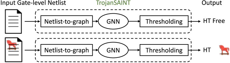
Figure 1: Concept of TrojanSAINT.

HT Localization. State-of-the-art GNN-based detection schemes, GNN4TJ [3] and HW2VEC [7], predict whether a design contains a HT or not, but they cannot localize HTs. However, localizing HTs is essential to identify the part of the design at fault and name the responsible, malicious party.

Scope. Earlier works [3, 7, 10] are limited to register transfer level (RTL), unable to handle gate-level netlists (GLNs). Such methods are restricted to pre-silicon assessment; they cannot detect HTs in the field. Note that only schemes which can work on GLNs allow for pre- and post-silicon detection.

Associated Research Challenges. Developing a GNN-based HT detection and localization scheme that can work on GLNs imposes the following research challenges (RC).

RC1: GLN Complexity. Compared to RTL, GLN designs are more complex to analyze, as GLNs are flattened (i.e., hierarchical information is lost) and also considerably larger, in the range of thousands or even millions of gates and wires.

RC2: Imbalanced Datasets. HTs are stealthy and small in size; HT gates represent a very small percentage, e.g., 0.14–11.29% or 1.94% on average for the TrustHub suite considered in this work. Thus, a highly imbalanced dataset arises (e.g., the ratio of regular to HT gates reaches up to 719$\times$ for the TrustHub suite), which is difficult to handle for any ML model.

Our Contributions. Here, we propose TrojanSAINT, a GNN-based method for HT detection and localization that works well on large-scale GLNs. The concept is outlined in Fig. 1.

As indicated, the graph representations of GLNs are complex and large, which makes them difficult to handle with traditional architectures such as graph convolutional networks (GCNs).

This motivates our decision to, without loss of generality (w/o.l.o.g.), use GraphSAINT [11] for our methodology. GraphSAINT is a well-established, sampling-based approach that extracts smaller sub-graphs for training from the larger original graph. It has shown good performance for various tasks [11, 12, 13], but it has not been considered for HT detection until now. We summarize our contributions as follows:

1. A parser for GLN-to-graph conversion (Sec. II-A) which performs feature extraction tailored for HT detection.

2. A GNN-based method for detection and localization of HT in GLNs (Sec. II-B), addressing RC1.

3. A procedure for tuning of the classification thresholds to obtain more accurate predictions, addressing RC2.

4. We demonstrate that our scheme is competitive to traditional ML baselines and prior art. We also verify the generalization ability of our scheme – i.e., good prediction accuracy for unknown HTs on unseen GLNs.

5. We open-source our scheme and related artifacts from our experimental study [https://github.com/DfX-NYUAD/TrojanSAINT].

II TrojanSAINT Methodology

An overview of our methodology is shown in Fig. 2. Next, we describe all relevant details.

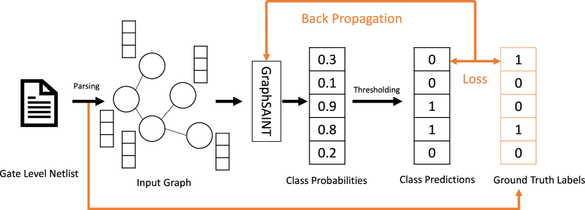
Figure 2: Overview of TrojanSAINT. Black arrows follow the inference process, orange arrows follow the additional steps needed for training and validation. In this example, the thresholding value is 0.4.

II-A GLN Parsing and Feature Vectors

Parser. We develop a parser that converts GLNs (given in Verilog format) into unweighted and undirected graphs, where nodes represent gates and edges represent wires. We are discarding directionality for improved representation learning [14]. Given a set of GLNs, our parser generates one large single graph, consisting of multiple disjoint graphs, where nodes are labeled as ‘train,’ ‘validation’ or ‘test,’ depending on the designation of the GLN they belong to. The graph is encoded as an adjacency matrix ${\bm{A}}$ following a standard procedure.

Feature Vectors. Our parser also generates a matrix ${\bm{X}}$ of feature vectors for all nodes. Vectors cover the following:

• Gate type, represented via one-hot encoding. From experimentation, we are more interested in the functionality of the gate over the exact implementation. That is, we group functionally related gates together, e.g., all AND gates are grouped regardless of the number of inputs and the driver strengths that the different AND gates support.

• Input, output degrees of gates, i.e., the number of incoming and outgoing connections.

• Shortest distances to primary inputs/outputs. For gates not directly connected with a primary input/output, a breadth-first search is conducted to obtain shortest distances.

For training and validation, we also use a binary label vector which marks each node as part of some HT or as regular/benign gate. The related information is derived during parsing.

II-B GNN Implementation and Application

Outline. We utilize GraphSAINT [11] for sampling. Further, we utilize the GNN architecture of GNN-RE [15], along with GraphSAGE [16]. We tune the classification thresholds for more accurate predictions. We further utilize a practical validation. For training and inference, we employ standard procedures.

GNN Architecture. We consider an undirected graph $\IfEq{}{}{\mathcal{G}}{\mathcal{G}}\left(\IfEq{}{}{\mathcal{V}}{\mathcal{V}},{\bm{A}}\right)$ for representing a GLN, where $\IfEq{}{}{\mathcal{V}}{\mathcal{V}}$ is the set of vertices/nodes/gates, and the adjacency matrix of the graph is ${\bm{A}}$, where $A_{u,v}=1$ and $A_{v,u}=1$ if there exists an edge/wire from vertex/gate $u$ to vertex/gate $v$. Each vertex $u$ in the initial graph $\IfEq{}{}{\mathcal{G}}{\mathcal{G}}$ has a feature vector $\bm{x}_{u}$. This vector represents the node embedding at layer zero of the GNN. The embedding of node $u$ is iteratively updated by the GNN, by aggregating the embedding of the node and its neighbors $\IfEq{}{}{\mathcal{N}}{\mathcal{N}}(u)$. The embedding of a node $u$ after $l$ GNN layers, $\bm{h}_{u}^{(l)}$, is given by:

$$\footnotesize\bm{a}_{u}^{(l)}=\text{AGGREGATE}^{(l)}\left(\left\{\bm{h}_{v}^{(l-1)}:v\in\mathcal{N}(u)\right\}\right)\vspace*{-5mm}$$ (1)

$$\footnotesize\bm{h}_{u}^{(l)}=\text{COMBINE}^{(l)}\left(\bm{h}_{u}^{(l-1)},\bm{a}_{u}^{(l)}\right)\vspace*{-5mm}$$ (2)

GNN architectures are defined by their implementation of AGGREGATE$(\cdot)$ and COMBINE$(\cdot)$. For example, GraphSAGE [16], which we also use here, works as follows:

$$\bm{h}_{u}^{(l)}=\sigma([\bm{W}_{l}\cdot AGG(\{\bm{h}_{v}^{(l-1)},\forall v\in\IfEq{}{}{\mathcal{N}}{\mathcal{N}}(u)\}),\bm{B}_{l}\bm{h}_{u}^{(l-1)}])$$ (3)

$$AGG=\sum_{v\in\IfEq{}{}{\mathcal{N}}{\mathcal{N}}(u)}\frac{\bm{h}_{v}^{(l-1)}}{|\IfEq{}{}{\mathcal{N}}{\mathcal{N}}(u)|}$$ (4)

where $\sigma(.)$ is an activation function such as ReLU and $\bm{W}_{l}$ and $\bm{B}_{l}$ are trainable weight matrices. In GraphSAGE, the embedding of node $\bm{h}_{u}^{(l)}$ is determined by first concatenating the node’s features from the previous layer $\bm{h}_{u}^{(l-1)}$ with the output of the AGG function. Then the $\bm{W}_{l}$ and $\bm{B}_{l}$ transformations learns the important components of the neighbors’ features and the node $u$, respectively. GraphSAGE is compatible with different $AGG$ functions. Here, we use the mean aggregator as described in Equation (4).

Thresholding. From experimentation, we observe that the classification threshold plays a significant role for prediction performance. This is because of the considerably imbalanced datasets (Sec. I, RC2), where the GNN model as is can predict the minority class, i.e., HT nodes, only with low confidence.

The goal of thresholding is to determine a sufficiently small value so that HT nodes/gates are classified as such the moment the GNN captures any hint of malicious structures. In other words, thresholding allows the GNN to focus more on the minority class, improving the performance of the entire model.

W/o.l.o.g., we tune the threshold between 0–0.5 in steps of 1,000 and select the threshold that yields the best score on validation. Here, best score refers to the average of true positive rate (TPR) and true negative rate (TNR).

Practical Validation. We propose an approach where predictions are made on unknown HTs residing within circuits that are neither seen during training nor have golden references. This represents a real-world scenario, where security engineers do not know in advance which HT to expect, if any at all, and further need to test circuits without golden references. Prior art did not necessarily consider such practical validation.

Training. First, we construct sub-graphs using a standard random-walk sampler (RWS). TrojanSAINT’s training procedure is shown in Algorithm 1. Due to the RWS, the network can become biased towards frequently sampled nodes. To alleviate this issue, we follow the normalization technique of [11]. We use stochastic gradient descent as optimizer. ${\IfEq{}{}{\mathcal{G}}{\mathcal{G}}}_{s}$ is sampled for each minibatch and a GNN is built on the sub-graph. The cross-entropy loss is calculated for each node in the sub-graph and the GNN weights are then updated by backpropagation.

Algorithm 1 TrojanSAINT training algorithm

1:Training graph $\IfEq{}{}{\mathcal{G}}{\mathcal{G}}\left(\IfEq{}{}{\mathcal{V}}{\mathcal{V}},{\bm{A}}\right)$; Ground truth $\overline{\bm{Y}}$; Sampler RWS

2:Trained GNN

3:Compute normalization coefficients $\alpha$, $\lambda$ using RWS

4:for each mini-batch do

5:    ${\IfEq{}{}{\mathcal{G}}{\mathcal{G}}}_{s}\left({\IfEq{}{}{\mathcal{V}}{\mathcal{V}}}_{s},{{\bm{A}}}_{s}\right)\leftarrow$ Sampled sub-graph of $\IfEq{}{}{\mathcal{G}}{\mathcal{G}}$ using RWS

6:    Build GNN on ${\IfEq{}{}{\mathcal{G}}{\mathcal{G}}}_{s}$

7:    $\left\{\bm{y}_{u}\;\middle|\;u\in\IfEq{}{}{\mathcal{V}}{\mathcal{V}}_{s}\right\}\leftarrow$ Propagating $\alpha$-normalized $\left\{\bm{x}_{u}\;\middle|\;u\in\IfEq{}{}{\mathcal{V}}{\mathcal{V}}_{s}\right\}$

8:    Propagating $\lambda$-normalized loss $L\left(\bm{y}_{u},\overline{\bm{y}}_{u}\right)$ to update weights

9:end for

Inference. See Algorithm 2. For all test nodes in the graph, node embeddings are calculated and passed to a fully-connected layer with softmax activation, to compute class probabilities. We then apply our thresholding technique, and finally convert class probabilities into labels.

Algorithm 2 TrojanSAINT inference algorithm

1:Flattened netlist $N$; Trained GNN; Threshold $th$

2:Trojan classification of all nodes/gates

3:Initiate $\IfEq{}{}{\mathcal{G}}{\mathcal{G}}\left(\IfEq{}{}{\mathcal{V}}{\mathcal{V}},{\bm{A}}\right)$ with $V\leftarrow GLN\_to\_graph(N)$

4:for each $u\in\IfEq{}{}{\mathcal{V}}{\mathcal{V}}$ do

5:    $\bm{z}_{u}\leftarrow GNN(u)$ $\triangleright$ Compute embedding

6:    $c_{u}\leftarrow fc({z}_{u},th)$ $\triangleright$ Classify node $u$ based on the threshold

7:end for

III Experimental Study

Table II: TPR/TNR Results for Practical Validation. Best Results, Considering Average of TPR and TNR, are Marked in Boldface.

TrustHub	All With Thresholding								Others Without Thresholding
Benchmark	TrojanSAINT	XGBoost	FCNN	GNN-RE	Logistic	Random	SVM		TrojanSAINT	XGBoost	FCNN	GNN-RE	Logistic	Random	SVM
					Regression	Forest							Regression	Forest
rs232t1000	1.00/0.60	1.00/0.57	0.85/0.64	0.77/0.51	1.00/0.46	0.69/0.75	N/A		1.00/0.60	0.23/0.91	0.00/1.00	0.00/1.00	0.00/1.00	0.15/0.92	0.00/1.00
rs232t1100	0.92/0.68	0.83/0.57	1.00/0.61	0.92/0.52	0.83/0.61	0.33/0.90	N/A		0.92/0.68	0.08/0.91	0.00/0.94	0.00/0.94	0.00/1.00	0.08/0.92	0.00/1.00
rs232t1200	0.41/0.80	0.59/0.56	0.59/0.91	0.82/0.27	0.71/0.60	0.35/0.75	N/A		0.41/0.80	0.06/0.90	0.06/1.00	0.06/0.93	0.00/1.00	0.00/0.91	0.00/1.00
rs232t1300	1.00/0.74	1.00/0.57	1.00/0.66	1.00/0.71	1.00/0.43	0.56/0.86	N/A		1.00/0.74	0.22/0.91	0.00/1.00	0.00/0.98	0.00/1.00	0.00/0.92	0.00/1.00
rs232t1400	0.92/0.50	0.92/0.57	1.00/0.56	1.00/0.27	1.00/0.46	0.54/0.70	N/A		0.92/0.50	0.08/0.91	0.08/0.71	0.62/0.94	0.00/1.00	0.00/0.92	0.00/1.00
rs232t1500	0.71/0.82	0.93/0.57	0.93/0.57	0.79/0.61	1.00/0.46	0.57/0.76	N/A		0.71/0.82	0.21/0.91	0.07/0.77	0.36/0.94	0.00/1.00	0.14/0.91	0.00/1.00
rs232t1600	0.73/0.57	0.73/0.57	0.91/0.49	0.55/0.66	0.73/0.59	0.27/0.90	N/A		0.73/0.57	0.18/0.91	0.00/1.00	0.00/0.83	0.00/1.00	0.00/0.91	0.00/1.00
s15850t100	0.35/0.97	0.77/0.94	0.92/0.76	0.88/0.97	0.96/0.73	0.85/0.94	N/A		0.35/0.97	0.12/1.00	0.00/1.00	0.12/1.00	0.00/1.00	0.04/1.00	0.04/1.00
s35932t100	1.00/1.00	0.87/0.98	0.87/0.64	0.93/1.00	0.93/0.44	1.00/0.98	N/A		1.00/1.00	0.20/1.00	0.00/1.00	0.00/0.97	0.00/1.00	0.13/1.00	0.07/1.00
s35932t200	1.00/1.00	1.00/0.98	0.92/0.80	1.00/1.00	0.92/0.44	1.00/0.99	N/A		1.00/1.00	0.00/1.00	0.00/1.00	0.00/1.00	0.00/1.00	0.00/1.00	0.00/1.00
s35932t300	0.97/1.00	0.94/0.98	1.00/0.81	1.00/1.00	0.40/0.81	0.97/0.97	N/A		0.97/1.00	0.63/1.00	0.00/1.00	0.09/1.00	0.00/1.00	0.57/1.00	0.00/1.00
s38417t100	0.92/0.92	1.00/0.82	0.75/0.77	1.00/0.92	1.00/0.35	0.75/0.90	N/A		0.92/0.92	0.33/0.95	0.00/1.00	0.00/1.00	0.00/1.00	0.42/0.94	0.00/1.00
s38417t200	0.40/0.99	0.53/0.86	0.73/0.73	0.47/0.93	1.00/0.35	0.73/0.90	N/A		0.40/0.99	0.27/0.95	0.73/0.90	0.00/1.00	0.00/1.00	0.27/0.94	0.00/1.00
s38417t300	0.98/0.96	0.98/0.82	0.18/0.89	0.98/0.91	0.16/0.87	0.95/0.84	N/A		0.98/0.96	0.14/0.95	0.07/1.00	0.00/0.98	0.02/1.00	0.23/0.95	0.07/1.00
s38584t100	1.00/0.95	1.00/0.87	1.00/0.87	1.00/0.92	1.00/0.52	1.00/0.93	N/A		1.00/0.95	0.22/1.00	0.00/1.00	0.00/1.00	0.00/1.00	0.22/1.00	0.00/1.00
s38584t200	0.90/0.98	0.49/0.87	0.89/0.87	0.39/0.95	0.98/0.52	0.84/0.94	N/A		0.90/0.98	0.02/1.00	0.00/1.00	0.00/1.00	0.00/1.00	0.02/1.00	0.02/1.00
s38584t300	0.13/0.98	0.08/0.88	0.47/0.94	0.23/0.93	0.94/0.52	0.45/0.94	N/A		0.13/0.98	0.01/1.00	0.00/1.00	0.00/1.00	0.00/1.00	0.01/1.00	0.00/1.00
Average	0.78/0.85	0.80/0.76	0.82/0.74	0.81/0.77	0.86/0.54	0.70/0.88	N/A		0.78/0.85	0.18/0.95	0.06/0.96	0.07/0.97	0.00/1.00	0.13/0.95	0.01/1.00

III-A Setup

Software. We use Python for coding and bash scripts for job/data management. TrojanSAINT extends on GNN-RE, which is obtained from [14] and is implemented in PyTorch. Our TrojanSAINT platform is available online [https://github.com/DfX-NYUAD/TrojanSAINT]. Baseline models are implemented using Scikit-Learn, except the fully-connected neural network (FCNN) in PyTorch.

Computation. Experiments for GNN-RE, TrojanSAINT and FCNN are conducted on a high-performance cluster with 4x Nvidia V100 GPUs and 360GB RAM; experiments for others are conducted on a workstation with Intel i7 CPU and 16GB RAM. Training of GNN-RE and TrojanSAINT takes $\approx$15–30 minutes per model, FCNN $\approx$10 minutes per model, and all others $\approx$3 minutes in total. All inference takes few seconds.

Benchmarks and Model Building. We use 17 exemplary GLN benchmarks from the TrustHub suite [17]. For each benchmark, a respective model is trained from scratch. For our practical validation, each model does not get to see the design to be tested at all during training.

We note that random seeds used in TrojanSAINT’s components affect performance significantly. Thus, we conduct w/o.l.o.g. 6 runs with different seeds and report only results for each model that performs best on its validation set.

Prior Art, Comparative Study. From Table I, recall that none of the prior art in GNN-based HT detection works on GLNs. Thus, a direct comparison is not practical. However, we consider the following works for comparison.

• GNN-RE [15]: Proposed for reverse engineering of GLNs, it could also be utilized for HT detection and localization. This is because GNN-RE seeks to classify gates/nodes from flattened GLNs into the circuit modules they belong to; TrojanSAINT’s task of classifying gates/nodes into begin or HT-infested ones is analogous.

• Related Works [18, 19, 20]: ML-based, not GNN-based, HT detection schemes that are working on GLNs. Unlike ours, these works employ elaborate feature engineering. Also, these works do not offer native HT localization.

We also implement and run the following well-known baseline classifiers for a further comparative study.

• XGBoost: A decision tree (DT)-based model that uses an ensemble of sequentially added DTs. DTs are added aiming to minimize errors of their predecessor.

• Random Forest: A DT-based model that uses an ensemble of DTs trained on subsets of the training data.

• Logistic Regression: A classification algorithm that utilizes the sigmoid function on independent variables.

• Support Vector Machine (SVM): A classification model that generates a hyperplane to separate different classes.

• FCNN: We implement a three-layer network; each layer use the SELU activation function [21] and batch normalization. The final layer uses sigmoid activation to calculate classification probabilities.

All these classifiers work on tabular, non-graph data; thus, we provide them with the feature vectors as inputs. All classifiers, except SVM, output probabilities; thus, we can study them considering our proposed thresholding as well.

III-B Results

Practical Validation and Impact of Thresholding. In Table II, we report TPR/TNR results for practical validation across two scenarios: with thresholding versus without.

First, the results show that TrojanSAINT outperforms other methods for this realistic but challenging scenario of HT detection considering unknown Trojans within unseen circuits. The GNN framework underlying of TrojanSAINT is superior to other models. Recall that others take the same feature vectors as inputs; such direct comparison is fair. Second, thresholding is crucial for high prediction performance for this task.

Relaxed Validation. We also study a “best case” validation, using a leave-one-out split where validation and test sets are the same. Such setting is often considered in the literature, as it shows the best performance for any model and benchmark. As indicated, however, it is not as realistic for HT detection.

With thresholding applied, we observe the following average TPR/TNR values here: 0.98/0.96 for TrojanSAINT, 0.93/0.93 for XGBoost, 0.91/0.89 for FCNN, 0.98/0.96 for GNN-RE, 0.89/0.81 for logistic regression, and 0.91/0.994 for random forest, respectively. Without thresholding applied, we observe the following average TPR/TNR values: 0.41/0.99 for XGBoost, 0.09/1.00 for FCNN, 0.07/0.97 for GNN-RE, 0.09/1.00 for logistic regression, 0.40/0.99 for random forest, and 0.11/1.00 for SVM, respectively. TrojanSAINT is superior to almost all methods across these two cases; only GNN-RE, and only with thresholding applied, becomes a close contender.

Related Works. In Table III, we compare to more loosely related works (Sec. III-A). Results are quoted and rounded. Numbers of nodes/gates are reported as obtained from our parser. The related works employ leave-one-out or “best case” validation schemes; thus, we also report TrojanSAINT results for such “best case” validation here.

Table III: Benchmark Properties; TPR/TNR Results for Related Works

TrustHub	Benign	HT	Ratio of Nodes,		R-HTD [18]	[19]	[20]	TrojanSAINT
Benchmark	Nodes	Nodes	HT to Benign		(Orig. Samples)
rs232t1000	202	13	0.064		1.00/0.94	1.00/0.99	1.00/1.00	1.00/0.94
rs232t1100	204	12	0.059		1.00/0.93	0.50/0.98	1.00/1.00	1.00/0.93
rs232t1200	199	17	0.085		0.97/0.96	0.88/1.00	1.00/1.00	0.82/0.96
rs232t1300	204	9	0.044		1.00/0.95	1.00/1.00	0.86/1.00	1.00/0.98
rs232t1400	202	13	0.064		1.00/0.98	0.98/1.00	1.00/1.00	1.00/0.96
rs232t1500	202	14	0.069		1.00/0.94	0.95/1.00	1.00/1.00	1.00/0.94
rs232t1600	203	11	0.054		0.97/0.92	0.93/0.99	0.78/0.99	1.00/0.88
s15850t100	2,156	26	0.012		0.74/0.93	0.78/1.00	0.08/1.00	0.88/0.97
s35932t100	5,426	15	0.003		0.80/0.69	0.73/1.00	0.08/1.00	1.00/0.97
s35932t200	5,426	12	0.002		0.08/1.00	0.08/1.00	0.08/1.00	1.00/1.00
s35932t300	5,427	35	0.006		0.84/1.00	0.81/1.00	0.92/1.00	1.00/1.00
s38417t100	5,329	12	0.002		0.67/1.00	0.33/1.00	0.09/1.00	1.00/0.97
s38417t200	5,329	15	0.003		0.73/0.99	0.47/1.00	0.09/1.00	1.00/0.97
s38417t300	5,329	44	0.008		0.89/1.00	0.75/1.00	1.00/1.00	1.00/0.96
s38584t100	6,473	9	0.001		N/A	N/A	0.17/1.00	1.00/0.99
s38584t200	6,473	83	0.013		N/A	N/A	0.18/1.00	1.00/0.98
s38584t300	6,473	731	0.113		N/A	N/A	0.03/1.00	0.99/0.95
Average	3,250	63	0.035∗		0.84/0.95	0.72/1.00	0.55/1.00	0.98/0.96
			0.019∗

^∗The first value is averaged across the column; the second value, more representative of the overall imbalance, is based on re-calculating the ratio using the average node counts.

TrojanSAINT outperforms these related works for all larger benchmarks, where the ratio of HT gates/nodes to regular ones is more challenging—this demonstrates superior scalability for ours. For the smaller benchmarks, which are not representative of real IC designs, related works achieve better results presumably due to feature engineering. In fact, up to 76 features are considered in [19, 20] which reflects on considerable efforts, whereas for ours, some simple feature vectors suffice.

IV Conclusion

We have developed TrojanSAINT, a GNN-based method for detection and localization of HTs. We overcome the HT-inherent issue of class imbalance through threshold tuning. Through practical validation, ours is capable of generalizing to circuits and HTs it has not seen for training. Our method outperforms prior art and a number of strong ML baselines. The use of a GNN framework renders TrojanSAINT simple yet competitive. For future work, we will study the role of different feature vectors in more details.

References

- [1] J. Rajendran, H. Zhang, O. Sinanoglu, and R. Karri, “High-level synthesis for security and trust,” in International On-Line Testing Symposium (IOLTS). IEEE, 2013, pp. 232–233.
- [2] R. Karri, J. Rajendran, K. Rosenfeld, and M. Tehranipoor, “Trustworthy hardware: Identifying and classifying hardware Trojans,” Computer, vol. 43, no. 10, pp. 39–46, 2010.
- [3] R. Yasaei, S.-Y. Yu, and M. A. Al Faruque, “GNN4TJ: Graph neural networks for hardware Trojan detection at register transfer level,” in Design, Automation & Test in Europe Conference & Exhibition (DATE). IEEE, 2021, pp. 1504–1509.
- [4] S. Faezi, R. Yasaei, and M. A. Al Faruque, “HTnet: Transfer learning for golden chip-free hardware Trojan detection,” in Design, Automation & Test in Europe Conference & Exhibition (DATE). IEEE, 2021, pp. 1484–1489.
- [5] J. He, Y. Liu, Y. Yuan, K. Hu, X. Xia, and Y. Zhao, “Golden chip free Trojan detection leveraging electromagnetic side channel fingerprinting,” IEICE Electronics Express, pp. 16–20 181 065, 2018.
- [6] K. Hasegawa, M. Yanagisawa, and N. Togawa, “Trojan-feature extraction at gate-level netlists and its application to hardware-trojan detection using random forest classifier,” in International Symposium on Circuits and Systems (ISCAS). IEEE, 2017, pp. 1–4.
- [7] S.-Y. Yu, R. Yasaei, Q. Zhou, T. Nguyen, and M. A. Al Faruque, “HW2VEC: A graph learning tool for automating hardware security,” in International Symposium on Hardware Oriented Security and Trust (HOST). IEEE, 2021, pp. 13–23.
- [8] L. Alrahis, S. Patnaik, M. Shafique, and O. Sinanoglu, “Embracing graph neural networks for hardware security,” in International Conference on Computer-Aided Design (ICCAD), IEEE/ACM. New York, NY, USA: Association for Computing Machinery, 2022. [Online]. Available: https://doi.org/10.1145/3508352.3561096
- [9] L. Alrahis, J. Knechtel, and O. Sinanoglu, “Graph neural networks: A powerful and versatile tool for advancing design, reliability, and security of ICs,” arXiv preprint arXiv:2211.16495, 2022.
- [10] R. Yasaei, S. Faezi, and M. A. Al Faruque, “Golden reference-free hardware Trojan localization using graph convolutional network,” IEEE Transactions on Very Large Scale Integration (VLSI) Systems, vol. 30, no. 10, pp. 1401–1411, 2022.
- [11] H. Zeng, H. Zhou, A. Srivastava, R. Kannan, and V. Prasanna, “Graphsaint: Graph sampling based inductive learning method,” arXiv preprint arXiv:1907.04931, 2019.
- [12] L. Alrahis, S. Patnaik, F. Khalid, M. A. Hanif, H. Saleh, M. Shafique et al., “GNNUnlock: Graph neural networks-based oracle-less unlocking scheme for provably secure logic locking,” in Design, Automation & Test in Europe Conference & Exhibition (DATE), 2021, pp. 780–785.
- [13] L. Alrahis, S. Patnaik, M. A. Hanif, H. Saleh, M. Shafique, and O. Sinanoglu, “GNNUnlock+: A systematic methodology for designing graph neural networks-based oracle-less unlocking schemes for provably secure logic locking,” IEEE Transactions on Emerging Topics in Computing, vol. 10, no. 3, pp. 1575–1592, 2022.
- [14] L. Alrahis. (2022) Gnn-re: Graph neural networks for reverse engineering of gate-level netlists. [Online]. Available: https://github.com/DfX-NYUAD/GNN-RE
- [15] L. Alrahis, A. Sengupta, J. Knechtel, S. Patnaik, H. Saleh, B. Mohammad et al., “GNN-RE: Graph neural networks for reverse engineering of gate-level netlists,” IEEE Transactions on Computer-Aided Design of Integrated Circuits and Systems, 2021.
- [16] W. Hamilton, Z. Ying, and J. Leskovec, “Inductive representation learning on large graphs,” Advances in neural information processing systems, vol. 30, 2017.
- [17] H. Salmani and M. Tehranipoor. (2021) Trust-hub: Chip-level Trojan benchmarks. [Online]. Available: https://trust-hub.org/#/benchmarks/chip-level-trojan
- [18] K. Hasegawa, S. Hidano, K. Nozawa, S. Kiyomoto, and N. Togawa, “R-htdetector: Robust hardware-trojan detection based on adversarial training,” 2022. [Online]. Available: https://arxiv.org/abs/2205.13702
- [19] K. Hasegawa, M. Yanagisawa, and N. Togawa, “Trojan-feature extraction at gate-level netlists and its application to hardware-trojan detection using random forest classifier,” in International Symposium on Circuits and Systems (ISCAS), 2017, pp. 1–4.
- [20] T. Kurihara and N. Togawa, “Hardware-trojan classification based on the structure of trigger circuits utilizing random forests,” in International Symposium on On-Line Testing and Robust System Design (IOLTS), 2021, pp. 1–4.
- [21] G. Klambauer, T. Unterthiner, A. Mayr, and S. Hochreiter, “Self-normalizing neural networks,” Advances in neural information processing systems, vol. 30, 2017.