Jet-veto resummation at ${}_{\text{p}}$+ in boson production processes

Abstract

Vetoing energetic jet activity is a crucial tool for suppressing backgrounds and enabling new physics searches at the LHC, but the introduction of a veto scale can introduce large logarithms that may need to be resummed. We present an implementation of jet-veto resummation for color-singlet processes at the level of N³LL${}_{\text{p}}$ matched to fixed-order predictions. Our public code MCFM allows for predictions of a single boson, such as $Z/\gamma^{*}$, $W^{\pm}$ or $H$, or with a pair of vector bosons, such as $W^{+}W^{-}$, $W^{\pm}Z$ or $ZZ$. The implementation relies on recent calculations of the soft and beam functions in the presence of a jet veto over all rapidities, with jets defined using a sequential recombination algorithm with jet radius $R$. However one of the ingredients that is required to reach full accuracy is only known approximately, hence N³LL${}_{\text{p}}$. We describe in detail our formalism and compare with previous public codes that operate at the level of NNLL. Our higher-order predictions improve significantly upon NNLL calculations by reducing theoretical uncertainties. We demonstrate this by comparing our predictions with ATLAS and CMS results.

1 Introduction

Jet vetoing is a crucial technique in particle physics that is used primarily to suppress backgrounds in processes involving the production of $W^{+}W^{-}$ final states (e.g. directly or in Higgs decays). By identifying and removing events that contain energetic hadronic jets (vetoing), the impact of the dominant top-quark pair production background is reduced. The concrete jet-veto implementation depends on factors such as the jet algorithm and its parameters, as well as the kinematic selection cuts applied to the identified jets. For LHC analyses, the most common jet vetoing scheme is to impose a maximum transverse momentum cut $p_{T}^{\rm veto}{}$ on anti-$k_{T}$ jets.

The jet veto scale $p_{T}^{\rm veto}{}$ can induce large logarithms if it is smaller than the hard process scale $Q$, which then mandates resummation. In this paper we describe a coherent implementation of jet veto resummation in processes involving the production of a color-singlet boson ($W,Z/\gamma^{*}$ and $H$ bosons) or a pair of bosons ($ZZ$, $W^{\pm}Z$, and $W^{+}W^{-}$). Our resummation operates at the level of N³LL${}_{\text{p}}$ matched to fixed order .

We build on the pioneering work of previous studies, which have demonstrated the effectiveness of resummation methods for a jet veto Berger:2010xi ; Stewart:2010tn ; Becher:2012qa ; Banfi:2012yh ; Banfi:2012jm . General purpose implementations include a numerical approach to resummation at +NNLL Kallweit:2020gva ; Re:2021con and an automated approach to jet veto studies at NLO+NNLL Becher:2014aya . Publicly available codes operating at NNLL and addressing the same issue are, JetVHeto JetHveto , the code MCFM-RE MCFM-RE which is derivative of both MCFM and JetVHeto, and MATRIX+RadISH Matrix+Radish . Both JetVHeto and RadISH implement the same analytic resummation formula of ref. Banfi:2012jm .

Our research extends and improves upon these earlier results through detailed phenomenological studies of specific final states, including Higgs boson production Banfi:2012jm ; Becher:2013xia ; Stewart:2013faa ; Banfi:2015pju , $W^{+}W^{-}$ production Dawson:2016ysj ; Arpino:2019fmo , and $ZZ$ and $W^{\pm}Z$ production Wang:2015mvz . Another important aspect of our study is the performance of the resummation at N³LL${}_{\text{p}}$ accuracy, which has not always been the case in previous work. We also describe our approximation of the missing $d_{3}^{{\rm veto}}$ that would be necessary to reach full accuracy. Finally, we include our results in MCFM, a publicly distributed code, which allows users to easily perform studies in practice.

Resummation of jet-veto logarithms has a close relationship with the resummation of transverse momentum logarithms. In the latter, one is interested in transverse momenta all the way down to zero $p_{T}$, so the logarithms can be larger than in jet-veto processes where $p_{T}^{\rm veto}$ in the range $2530\text{\,}\mathrm{GeV}$ is used experimentally. In this paper we explore which jet-veto processes actually require resummation at these values of $p_{T}^{\rm veto}$, supply the best predictions for those processes where it is warranted, and confront our theoretical predictions with experimental data where it is available.

In Section 2 we discuss the jet-veto factorization theorem including its ingredients that result in the resummation. We describe our setup for phenomenology including our uncertainty procedure in Section 3, compare with the public code JetVHeto in Section 4, and study the phenomenological implications for a wide range of processes in Section 5. We conclude in Section 6.

2 Jet-veto factorization and resummation

We consider processes where jets have been defined using sequential recombination jet algorithms Salam:2010nqg with distance measure

$$d_{ij}=\mbox{min}(k_{Ti}^{2n},k_{Tj}^{2n})\,\frac{\Delta y_{ij}^{2}+\Delta\phi_{ij}^{2}}{R^{2}}\,,\qquad d_{iB}=k_{Ti}^{2n}\,,$$ (1)

where the choice $n=-1$ is the anti-$k_{T}$ algorithm Cacciari:2008gp , $n=0$ is the Cambridge-Aachen algorithm Dokshitzer:1997in ; Wobisch:1998wt , and $n=1$ is the $k_{T}$ algorithm Catani:1993hr ; Ellis:1993tq . $k_{Ti}$ denotes the transverse momentum of (pseudo-)particle $i$ with respect to the beam direction, and $\Delta y_{ij}$ and $\Delta\phi_{ij}$ are the rapidity and azimuthal angle differences of (pseudo-)particles $i$ and $j$.

To describe the resummation method we focus on the simplest case of quark-antiquark induced Drell-Yan production of a lepton pair of invariant mass $Q$ and rapidity $y$. The case of gluon initiated processes is structurally the same, but with different ingredients that we give below and in the appendices. In the presence of a jet veto over all rapidities we have a factorization formula Becher:2012qa ; Becher:2013xia ; Stewart:2013faa ,

$$\frac{d^{2}\sigma(p_{T}^{\rm veto})}{dQ^{2}dy} =\frac{d\sigma_{0}}{dQ^{2}}\,\left|C^{V}(-Q^{2},\mu)\right|^{2}$$

$$\times\Big{[}{\cal B}_{q}(\xi_{1},Q,p_{T}^{\rm veto},R,\mu,\nu)\,{\cal B}_{\bar{q}}(\xi_{2},Q,p_{T}^{\rm veto},R,\mu,\nu)\,{\cal S}(p_{T}^{\rm veto},R,\mu,\nu)\Big{]}+\mathcal{O}\left(\frac{p_{T}^{\rm veto}}{Q}\right)$$ (2)

where $\xi_{1,2}=(Q/\sqrt{s})\,e^{\pm y}$ and,

$$\frac{d\sigma_{0}}{dQ^{2}}=\frac{4\pi\alpha^{2}}{3N_{c}Q^{2}s}\,.$$ (3)

In this equation $C^{V}$ is a matching coefficient whose square is the hard coefficient function that corrects the lowest order cross-section, see Eq. 3. ${\cal B}_{q}$ and ${\cal B}_{\bar{q}}$ are the quark beam functions which describe the emission of radiation collinear to the two beam directions in the presence of a jet veto, and ${\cal S}$ describes the emission of soft radiation in the presence of a jet veto. The quantity $\nu$ is a supplementary scale necessitated by the rapidity divergences present in beam and soft functions. The main process-independent ingredients are the beam and soft functions for both incoming quarks and gluons which have been published recently at the two-loop level Abreu:2022zgo ; Abreu:2022sdc . The hard function is process specific. We have used the existing two-loop fixed order implementations in MCFM.

Overall the factorization theorem achieves a separation of scales. The hard function contains logarithms of the ratio $Q^{2}/\mu^{2}$, which can be minimized by setting $\mu^{2}=\mu_{h}^{2}\sim Q^{2}$. However, inside the beam and soft functions, it is natural to choose $\mu=p_{T}^{\rm veto}$ to avoid large logarithms. The resummation of large logarithms is achieved by choosing $\mu\sim Q$ in the hard function and evolving it down to the resummation scale $\mu\sim p_{T}^{\rm veto}$ using the renormalization group (RG). For the hard function the evolution is solved analytically, see Appendix E.

In RG-improved power counting the logarithms $L_{\perp}=2\log(\mu_{h}/p_{T}^{\rm veto})$, where $\mu_{h}$ is of order $Q$, are assumed to be of order $1/\alpha_{s}$. With this definition the counting of powers of $\alpha_{s}$ and of the large logarithm $L_{\perp}$ is shown in Table 1.

Table 1: Counting of orders in the resummation, adapted from ref. Becher:2006mr . The second column indicates the nominal order when counting $L_{\perp}\sim 1/\alpha_{s}$. The third column states which logarithms are included. The last three columns show the necessary additional anomalous dimensions and hard function corrections in each successive order. The requisite anomalous dimensions are provided in Appendix B.

Approximation	Nominal order	Accuracy $\sim\alpha_{s}^{n}L_{\perp}^{k}$	$\Gamma_{\text{cusp}}$	$\gamma_{\text{coll.}}$	$H$
LL	$\alpha_{s}^{-1}$	$2n\geq k\geq n+1$	$\Gamma_{0}$	tree	tree
NLL+LO	$\alpha_{s}^{0}$	$2n\geq k\geq n$	$\Gamma_{1}$,	$\gamma_{0}$	tree
N2LL+NLO	$\alpha_{s}^{1}$	$2n\geq k\geq\text{max}(n-1,0)$	$\Gamma_{2}$	$\gamma_{1}$	1-loop
N3LL +NNLO	$\alpha_{s}^{2}$	$2n\geq k\geq\text{max}(n-2,0)$	$\Gamma_{3}$	$\gamma_{2}$	2-loop

The non-logarithmic terms that the resummation does not provide are easily accounted for by adding the matching corrections. The matching corrections are a finite contribution and add the effect of fixed-order corrections while removing the logarithmic overlap through a fixed-order expansion of the resummation.

2.0.1 Soft function

The jet veto soft function has been calculated using an exponential regulator Li:2016axz in Ref. Abreu:2022sdc . The calculation is divided into the sum of the soft function for a reference observable and a correction factor,

$$S(p_{T}^{\rm veto},R,\mu,\nu)=S_{\perp}(p_{T}^{\rm veto},\mu,\nu)+\Delta S(p_{T}^{\rm veto},R,\mu,\nu)\,.$$ (4)

In Ref. Abreu:2022sdc the reference observable is the transverse momentum of the color singlet system denoted by $S_{\perp}$. $S_{\perp}$ can be derived from the expression given in Refs. Vladimirov:2016dll ; Li:2016ctv after performing the Fourier transform to momentum space (see, for instance, the rules given in Table 1 of Ref. Billis:2019vxg ). $\Delta S$ depends on the jet algorithm and contributes for two or more emissions. It thus depends only on double real emission diagrams.

2.0.2 Refactorization and reduced beam functions

For consistency with the transverse momentum resummation framework in CuTe-MCFM Becher:2020ugp we cast the factorization theorem in terms of the collinear anomaly framework. In this framework the rapidity logarithms are exponentiated directly instead of resummed by solving rapidity RG equations Chiu:2012ir ; Chiu:2011qc . For this we rewrite the square bracket in Eq. 2 as follows,

$${\cal B}_{q}(\xi_{1},Q,p_{T}^{\rm veto},R,\mu,\nu)\,{\cal B}_{\bar{q}}(\xi_{2},Q,p_{T}^{\rm veto},R,\mu,\nu){\cal S}(p_{T}^{\rm veto},R,\mu,\nu)$$

$$=\left(\frac{Q}{p_{T}^{\rm veto}}\right)^{-2F_{qq}(p_{T}^{\rm veto},R,\mu)}e^{2h^{F}(p_{T}^{\rm veto},\mu)}\,\bar{B}_{q}(\xi_{1},p_{T}^{\rm veto},R,\mu)\,\bar{B}_{\bar{q}}(\xi_{2},p_{T}^{\rm veto},R,\mu)\,.$$ (5)

The $\nu$ dependence vanishes in this combination of beam and soft functions.

We have factored out $e^{h^{F/A}(p_{T}^{\rm veto},\mu)}$ from each beam function, resulting in the reduced beam functions $\bar{B}$. By construction $h^{F/A}$ are solutions of the RGE equation,

$$\frac{d}{d\ln\mu}\,h^{F/A}(p_{T}^{\rm veto},\mu)=2\Gamma_{\rm cusp}^{F/A}(\mu)\,\ln\frac{\mu}{p_{T}^{\rm veto}}-2\gamma^{q/g}(\mu)\,,$$ (6)

with boundary condition $h^{F/A}(\mu,\mu)=0$. The superscripts $F$ or $A$ signify whether the color is treated in the fundamental ($F$) or adjoint ($A$) representation, corresponding to a quark initiated process or a gluon initiated process, respectively. The exact form of $h^{F/A}(p_{T}^{\rm veto},\mu)$, determined by solving Eq. (6), is given in Appendix C.1. In terms of the reduced beam functions the jet-vetoed cross-section is now given by,

$$\frac{d^{2}\sigma(p_{T}^{\rm veto})}{dQ^{2}dy}=\frac{d\sigma_{0}}{dQ^{2}}\,\bar{H}(Q,\mu,p_{T}^{\rm veto})\bar{B}_{q}(\xi_{1},p_{T}^{\rm veto},R,\mu)\,\bar{B}_{\bar{q}}(\xi_{2},p_{T}^{\rm veto},R,\mu)+\mathcal{O}(p_{T}^{\rm veto}/Q)\,,$$ (7)

The choice of $h^{F/A}$ in Eq. 6 divides Eq. 2 into two separately RG invariant pieces, the product of the two reduced beam functions ($\bar{B}_{q}\,\bar{B}_{\bar{q}}$), and the hard function, ($\bar{H}$)

$$\bar{H}(Q,\mu,p_{T}^{\rm veto})=\left|C^{V}(-Q^{2},\mu)\right|^{2}\left(\frac{Q}{p_{T}^{\rm veto}}\right)^{-2F_{qq}(p_{T}^{\rm veto},R,\mu)}\,e^{2h^{F}(p_{T}^{\rm veto},\mu)}\,.$$ (8)

For quark-initiated processes the functions $C^{V}$ and $F_{qq}$ obey the following RG equations.

$$\frac{d}{d\ln\mu}\,C^{V}(-Q^{2},\mu) =\Big{[}\Gamma_{\rm cusp}^{F}(\mu)\,\ln\frac{-Q^{2}}{\mu^{2}}+2\gamma^{q}(\mu)\Big{]}C^{V}(-Q^{2},\mu)\,,$$ (9)

$$\frac{d}{d\ln\mu}F_{qq}(p_{T}^{\rm veto},R,\mu) =2\Gamma_{\mathrm{cusp}}^{F}(\mu)\,.$$ (10)

Eqs. 9 and 10 are structurally the same for the gluon case with different anomalous dimensions.

The function $\bar{H}$ is RG invariant due to the RGE’s satisfied by $C^{V}$ and $F_{qq}$ and $h_{F}$:

$$\frac{d}{d\mu}\bar{H}(Q,\mu,p_{T}^{\rm veto})=\mathcal{O}(\alpha_{s}^{3})\,.$$

Consequently, the remaining product of reduced beam functions is also RG invariant, up to the order calculated. In our case,

$$\frac{d}{d\mu}\bar{B}_{q}(\xi_{1},p_{T}^{\rm veto},R,\mu)\,\bar{B}_{\bar{q}}(\xi_{2},p_{T}^{\rm veto},R,\mu)=\mathcal{O}(\alpha_{s}^{3})\,.$$ (11)

The confirmation of Eq. 11 and the confirmation of the $R$-dependence of the collinear anomaly given in the next section are two simple checks of the results of Refs. Abreu:2022zgo ; Abreu:2022sdc . Full details of the formulas needed to perform this check are given in Appendix C.

If the scale $p_{T}^{\rm veto}$ is in the perturbative domain, the reduced beam function can be written in terms of the matching kernels $\bar{I}$ as

$$\bar{B}_{i}(\xi,p_{T}^{\rm veto},R,\mu)=\sum_{j=g,q,\bar{q}}\int_{\xi}^{1}\!\frac{dz}{z}\,\bar{I}_{ij}(z,p_{T}^{\rm veto},R,\mu)\,\phi_{j/P}(\xi/z,\mu)\,,$$

where $\phi$ denotes the usual collinear parton distribution of a parton of flavor $j$ in a proton $P$. The matching coefficients $\bar{I}$ are extracted from $I$, the two-loop beam and soft functions of Refs. Abreu:2022zgo ; Abreu:2022sdc as,

$$\bar{I}_{ij}(z,p_{T}^{\rm veto},R,\mu)=e^{-h^{F/A}(p_{T}^{\rm veto},\mu)}\,I_{ij}(z,p_{T}^{\rm veto},R,\mu)\,.$$ (12)

The coefficients in Ref. Abreu:2022zgo are presented as a Laurent expansion in the jet radius parameter $R$. Analytic expressions are presented for all flavor channels except for a set of $R$-independent non-logarithmic terms which are presented as numerical grids. For our purposes we have interpolated the numerical grids using a spline fit. We give further details on the reduced beam functions in Appendix A.

2.1 The collinear anomaly coefficient and its approximations

The missing ingredient for a complete resummation is the three-loop collinear anomaly coefficient and therefore warrants a longer discussion. This limitation has been discussed in the literature and approximated in various ways. Here we discuss the uncertainty associated with the approximations and how we take it into account in our phenomenological predictions.

As presented in Eq. 10 the collinear anomaly coefficients obey the RG equations,

$$\frac{d}{d\ln\mu}F_{qq}(p_{T}^{\rm veto},R,\mu) =2\Gamma^{F}_{\mathrm{cusp}}(\mu)\,,$$ (13)

$$\frac{d}{d\ln\mu}F_{gg}(p_{T}^{\rm veto},R,\mu) =2\Gamma^{A}_{\mathrm{cusp}}(\mu)\,,$$ (14)

where, for example, $F_{qq}$ has the expansion,

$$F_{qq}(p_{T}^{\rm veto},R,\mu) =\frac{\alpha_{s}}{4\pi}F_{qq}^{(0)}(p_{T}^{\rm veto},R,\mu)+\left(\frac{\alpha_{s}}{4\pi}\right)^{2}F_{qq}^{(1)}(p_{T}^{\rm veto},R,\mu)$$

$$+\left(\frac{\alpha_{s}}{4\pi}\right)^{3}F_{qq}^{(2)}(p_{T}^{\rm veto},R,\mu)+\left(\frac{\alpha_{s}}{4\pi}\right)^{4}F_{qq}^{(3)}(p_{T}^{\rm veto},R,\mu)+\ldots$$ (15)

While the logarithmic structure is given by the RG equations, the constant boundary parts $d_{k}^{\rm veto}(R,B)$ where $B=F$ or $A$ need to be determined by separate calculations and are also referred to as the rapidity anomalous dimensions in the framework of Refs. Chiu:2012ir ; Chiu:2011qc :

$$F_{qq}^{(0)}(p_{T}^{\rm veto},R,\mu_{h}) = \Gamma_{0}^{F}L_{\perp}+d_{1}^{\rm veto}(R,F)\,,$$

$$F_{qq}^{(1)}(p_{T}^{\rm veto},R,\mu_{h}) = \frac{1}{2}\Gamma_{0}^{F}\*\beta_{0}\*L_{\perp}^{2}+\Gamma_{1}^{F}\*L_{\perp}+d_{2}^{{\rm veto}}(R,F)\,,$$

$$F_{qq}^{(2)}(p_{T}^{\rm veto},R,\mu_{h}) = \frac{1}{3}\Gamma_{0}^{F}\*\beta_{0}^{2}\*L_{\perp}^{3}+\frac{1}{2}(\Gamma_{0}^{F}\*\beta_{1}+2\*\Gamma_{1}^{F}\*\beta_{0})\*L_{\perp}^{2}$$

$$+ (\Gamma_{2}^{F}+2\*\beta_{0}\*d_{2}^{{\rm veto}}(R,F))\*L_{\perp}+d_{3}^{{\rm veto}}(R,F)\,,$$

$$F_{qq}^{(3)}(p_{T}^{\rm veto},R,\mu_{h}) = \frac{1}{4}\*\beta_{0}^{3}\*\Gamma_{0}^{F}\*L_{\perp}^{4}+(\Gamma_{1}^{F}\*\beta_{0}^{2}+\frac{5}{6}\*\Gamma_{0}^{F}\*\beta_{0}\*\beta_{1})\*L_{\perp}^{3}$$ (16)

$$+ (\frac{1}{2}\*\Gamma_{0}^{F}\*\beta_{2}+\Gamma_{1}^{F}\*\beta_{1}+\frac{3}{2}\*\Gamma_{2}^{F}\*\beta_{0}+3\*d_{2}^{{\rm veto}}(R,F)\*\beta_{0}^{2})\*L_{\perp}^{2}$$

$$+ (\Gamma_{3}^{F}+3\*d_{3}^{{\rm veto}}(R,F)\*\beta_{0}+2\*d_{2}^{{\rm veto}}(R,F)\*\beta_{1})L_{\perp}+d_{4}^{{\rm veto}}(R,F)\,.$$

The analogous expression for gluons ($F\to A$) is given in Eq. (D). The coefficients in the expansion of the cusp anomalous dimension, $\Gamma_{k}^{F}$, are given in Appendix B.2.

For single gluon emission $d_{1}^{\rm veto}(R,B)=0$. The function $d_{2}^{{\rm veto}}$ is defined below in Section 2.1. There is only partial information on $d_{3}^{{\rm veto}}$ from Refs. Alioli:2013hba ; Dasgupta:2014yra ; Banfi:2015pju , and we have to rely on an approximation. To estimate the validity of this approximation we first study similar approximations of $d_{2}^{\rm veto}$.

The function $d_{2}^{{\rm veto}}$ is given by Becher:2013xia ,

$$d_{2}^{{\rm veto}}(R,B) =d_{2}^{B}-32C_{B}\,f(R,B)\,,\text{ where }$$

$$d_{2}^{B} =C_{B}\left[\left(\frac{808}{27}-28\zeta_{3}\right)C_{A}-\frac{224}{27}\,T_{F}n_{f}\right].$$ (17)

The function $f(R,B)$, which gives the dependence on the jet radius $R$, is known as an expansion about $R=0$ up to terms including $R^{4}$,

$$f(R,B) = C_{B}\Big{(}-\frac{\pi^{2}R^{2}}{12}+\frac{R^{4}}{16}\Big{)}$$ (18)

$$+ C_{A}\,\Big{(}c_{L}^{A}\ln R+c_{0}^{A}+c_{2}^{A}R^{2}+c_{4}^{A}R^{4}+\dots\Big{)}$$

$$+ T_{F}n_{f}\,\Big{(}c_{L}^{f}\ln R+c_{0}^{f}+c_{2}^{f}R^{2}+c_{4}^{f}R^{4}+\dots\Big{)}\,.$$

The terms on the first line are due to independent emission, whereas the terms on the second and third lines are due to correlated emission Banfi:2012yh . The expansion coefficients are given in Appendix D in analytic and numerical form.

2.1.1 Approximations for $d_{2}^{{\rm veto}}$

Using Sections 2.1 and 104 we have for the gluon case in the limit $n_{f}\to 0$ and retaining only logarithmic and constant terms in $R$,

$$d_{2}^{{\rm veto}}(R,A) =-32C_{A}^{2}\Big{[}-\frac{1}{32C_{A}^{2}}d_{2}^{A}+c_{L}^{A}\ln R+c_{0}^{A}\Big{]}$$

$$\simeq-32C_{A}^{2}\Big{[}-1.096259\ln R+0.7272641]$$

$$\sim 32C_{A}^{2}\times\ln\Big{(}\frac{R}{2}\Big{)}\,.$$ (19)

This result was used as a basis for an approximation to $d_{3}^{{\rm veto}}$ in ref. Becher:2013xia . However, the leading color ($n_{f}=0$) approximation is rather poor. With full $n_{f}$ dependence, but retaining only logarithmic and constant terms in $R$ and setting $n_{f}=5$ we have

$$d_{2}^{{\rm veto}}(R,B) = 32C_{B}C_{A}\Big{[}(1.096+0.0295n_{f})\*\ln R-(0.72726+0.12445n_{f})\Big{]}$$ (20)

$$\sim 32C_{B}C_{A}\Big{[}1.2435\ln\Big{(}\frac{R}{2.96}\Big{)}\Big{]}.$$

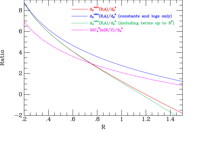
Figure 1: Approximations of $d_{2}^{{\rm veto}}(R,A)$ scaled by the constant $d_{2}^{A}$. The full result, Eq. (2.1) is plotted in red. The approximation retaining only constant terms and logarithms of $R$ is shown in blue. The approximation retaining constant terms and logarithms of $R$ and $R^{2}$ terms is shown in green. The leading color ansatz, Eq. (2.1.1), derived setting $n_{f}=0$, is $32C_{A}^{2}\ln(R/2)$ and is shown in magenta. The red, blue and green curves are all plotted for $n_{f}=5$.

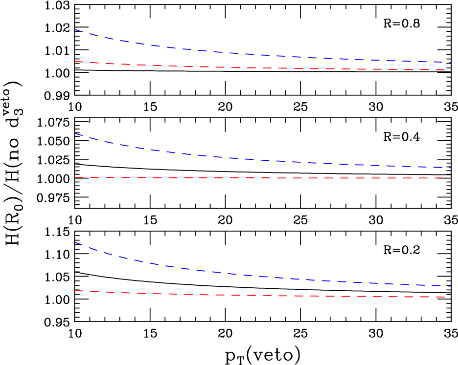
Figure 2: Effect of $R_{0}$ variation in $d_{3}^{\rm veto}$ as given by Eq. (24) with $Q=125$ GeV and $n_{f}=5$, compared to the case $d_{3}^{{\rm veto}}=0$: $R_{0}=1$ (black), $R_{0}=0.5$ (red, dashed), $R_{0}=2$ (blue, dashed).

In Fig. 1 we show $d_{2}^{{\rm veto}}(R,A)$ and its approximations in units of $d_{2}^{A}$ as a function of the jet radius $R$. As a reminder, $d_{2}^{A}$ is the non-$R$ dependent part of $d_{2}$, see Section 2.1. We first compare the full result (red) with the inclusion of terms up order $R^{2}$ (green). This shows that the $R$ expansion converges quickly and it is sufficient to consider only terms up to $R^{4}$ for practical applications. Including only the logarithm and the constant (blue) gives a reasonable approximation for sufficiently small $R$, with percent-level deviations around $R=0.4$. The leading color approximation (magenta) works only crudely as a first guess and could be used in the absence of any better estimate.

2.1.2 The function $d_{3}^{{\rm veto}}$

While the complete $d_{3}^{{\rm veto}}$ is unknown so far, we can extract the leading logarithmic term from results in the literature. Given that this approximation works reasonably well for $d_{2}^{\text{veto}}$ for $R\sim 0.4$, it is reasonable to expect a similar behavior for $d_{3}^{{\rm veto}}$. We further estimate the uncertainty associated with such an approximation.

From Eq. 15 the collinear anomaly coefficient at $\mu=p_{T}^{\rm veto}$ is given by,

$$F_{gg}(p_{T}^{\rm veto},R,p_{T}^{\rm veto})=\left(\frac{\alpha_{s}}{4\pi}\right)^{2}d_{2}^{{\rm veto}}(R,A)+\left(\frac{\alpha_{s}}{4\pi}\right)^{3}d_{3}^{{\rm veto}}(R,A)+\ldots$$ (21)

Therefore, expanding the collinear anomaly we have that

$$\Big{(}\frac{Q}{p_{T}^{\rm veto}}\Big{)}^{-2F_{gg}(p_{T}^{\rm veto},p_{T}^{\rm veto})}= 1-2\left(\frac{\alpha_{s}(p_{T}^{\rm veto})}{4\pi}\right)^{2}\ln\left(\frac{Q}{p_{T}^{\rm veto}}\right)d_{2}^{{\rm veto}}(R,A)$$

$$-2\ln\left(\frac{\alpha_{s}(p_{T}^{\rm veto})}{4\pi}\right)^{3}\ln\left(\frac{Q}{p_{T}^{\rm veto}}\right)d_{3}^{{\rm veto}}(R,A)\,+{\cal O}(\alpha_{s}^{4}).$$ (22)

At order $\alpha_{s}^{3}$ the leading term in the limit $R\to 0$ can be extracted from Eq. (C.2) of Ref. Banfi:2015pju which reads,

$$\mathcal{F}^{\text{correl}}_{\text{LL${}_{R}$},31}(R)=\left(\frac{\alpha_{s}}{4\pi}\right)^{3}\ln\Big{(}\frac{Q}{p_{T}^{\rm veto}}\Big{)}\cdot 128C_{A}\ln^{2}\frac{R}{R_{0}}$$

$$\times\Big{[}1.803136C_{A}^{2}-0.589237n_{f}2T_{R}C_{A}+0.36982C_{F}n_{f}2T_{R}-0.05893n_{f}^{2}4T_{R}^{2}\Big{]}\,.$$ (23)

Comparing the third-order coefficient in the two equations we thus have for a general color representation

$$d_{3}^{{\rm veto}}(R,B) =-64C_{B}\ln^{2}\Big{(}\frac{R}{R_{0}}\Big{)}(1.803136C_{A}^{2}+0.36982C_{F}n_{f}-0.589237C_{A}n_{f}-0.05893n_{f}^{2})$$

$$=-8.38188\times 64C_{B}\ln^{2}\Big{(}\frac{R}{R_{0}}\Big{)}~{}\mbox{for}~{}n_{f}=5\,.$$ (24)

Hence, the sign of the leading term in the small $R$ limit is known. In this limit $d_{3}^{{\rm veto}}$ leads to an increase in the cross-section. This approximation only gives the leading $R$ behavior, and it has been suggested that one may plausibly take $\frac{1}{2}<R_{0}<2$ as an uncertainty envelope Banfi:2015pju .

Since $d_{3}^{{\rm veto}}$ enters through the collinear anomaly as an overall factor, we consider the impact of varying $R_{0}$ in Fig. 2. For typical values of $p_{T}^{\rm veto}=$30\text{\,}\mathrm{GeV}$$ (as considered in this paper for the comparison with experimental studies) there is an effect of less than two percent for $R=0.4$. This is in agreement with the deviations we found for $d_{2}^{\text{veto}}$ for this approximation.

We take into account this variation in our uncertainty estimates, see Section 3.3. A definitive statement on this issue will have to await an exact calculation of $d_{3}^{{\rm veto}}$.

3 Setup for phenomenology

Before discussing phenomenological results, we list our input parameters, the method for matching to fixed order, and the approach for estimating uncertainties at fixed order and at the resummed level.

3.1 Input parameters

The input values used in our numerical studies are shown in Table 2. As indicated in the table we use the complex mass scheme for the $W$ and $Z$ boson masses. The number of light quarks, $n_{f}$, is set equal to five, except for the case of $W^{+}W^{-}$-production where $n_{f}=4$. We use the PDF distribution NNPDF31_nnlo_as_0118 except for $W^{+}W^{-}$ where we use NNPDF31_nnlo_as_0118_nf_4 NNPDF:2017mvq . Note that we use these parton distributions even in our lower order predictions.

Table 2: Input and derived parameters used for our numerical estimates.

$M_{W}$	80.385 GeV	$\Gamma_{W}$	2.0854 GeV
$M_{Z}$	91.1876 GeV	$\Gamma_{Z}$	2.4952 GeV
$G_{\mu}$	$1.166390\times 10^{-5}$ GeV-2
$m_{t}$	173.2 GeV	$m_{h}$	125 GeV
$m_{W}^{2}=M_{W}^{2}-iM_{W}\Gamma_{W}$	$(6461.748225-167.634879\,i)$ GeV2
$m_{Z}^{2}=M_{Z}^{2}-iM_{Z}\Gamma_{Z}$	$(8315.17839376-227.53129952\,i)$ GeV2
$\cos^{2}\theta_{W}={m_{W}^{2}}/{m_{Z}^{2}}$	$(0.7770725897054007+0.001103218322282256\,i)$
$\alpha=\frac{\sqrt{2}G_{\mu}}{\pi}M_{W}^{2}(1-\frac{M_{W}^{2}}{M_{Z}^{2}})$	$7.56246890198475\times 10^{-3}$ giving $1/\alpha\approx 132.23\ldots$

In the cases of $WW$ and $ZZ$ production, at ${\cal O}(\alpha_{s}^{2})$ the cross-section receives contributions from processes with two gluons in the initial state. When performing the resummed calculations we include such contributions at NLL relative to the leading order, which is of order $\alpha_{s}^{2}$. For the complete process the terms included are of order $\alpha_{s}^{n}L^{k}$ with $2n-4>k>\max(n-2,0)$ and hence they contribute at $\NNNLL$. Because of the large flux of gluons, one might worry that this formal counting is not appropriate. However, these contributions only represent about 3% of the cross-section for $p_{T}^{\rm veto}=10$ GeV, rising to about 6–8% for $p_{T}^{\rm veto}=60$ GeV. Therefore, neglecting higher order corrections to these contributions, which are not implemented in our code, is justified.

We match the resummation and fixed-order N^kLO corrections using a naive additive scheme as follows,

$$\sigma^{\text{N${}^{(k+1)}$LL+N${}^{(k)}$LO}}(p_{T}^{\rm veto}) =\sigma^{\text{N${}^{(k+1)}$LL}}(p_{T}^{\rm veto})+\sigma^{\Delta,k}(p_{T}^{\rm veto})\,,\text{ where}$$ (25)

$$\sigma^{\Delta}(p_{T}^{\rm veto}) =\sigma^{\text{N${}^{k}$LO}}(p_{T}^{\rm veto})-\mathrm{d}\sigma^{\text{N${}^{(k+1)}$LL}}(p_{T}^{\rm veto})\bigg{|}_{\text{exp. to {\text{N${}^{k}$LO}}}}.$$ (26)

The matching correction $\sigma^{\Delta}(p_{T}^{\rm veto})$ is defined as a function of $p_{T}^{\rm veto}$, using the difference between the fixed-order contribution and the resummed result expanded to the same fixed order. The limit $p_{T}^{\rm veto}\to 0$ of $\sigma^{\Delta}(p_{T}^{\rm veto})$ is finite, which also allows its use as a higher-order subtraction scheme.

The use of a naive matching without a transition mechanism that switches off the resummation at large $p_{T}^{\rm veto}$ is justified since the matching corrections for all considered cases in this paper are small; even in the most extreme case they are less than $20\%$. In other words, the resummation alone provides a good description of the cross-sections and does not need to be switched off. Any transition function to turn off the resummation at large $p_{T}^{\rm veto}$ would have a very small effect. This is in contrast to transverse-momentum resummation where a transition function is necessary Becher:2020ugp .

3.2 Uncertainty estimates at fixed order

Ultimately the resummed predictions should offer a practical advantage compared to the fixed-order predictions. In many cases, the quantity $\log(Q/p_{T}^{\rm veto})$ is not very large, and it may not seem worthwhile to use resummed results. However, as we will show, the resummation works remarkably well on its own and has matching corrections of only up to around 20%, often much less. The clear separation of scales and the resummation then allow for smaller and more reliable uncertainty estimates. To set the stage, we first examine perturbative convergence and uncertainties at fixed order for quark and gluon induced boson processes, as well as for $WW$ and $ZZ$ production.

Constructing jet-vetoed cross-sections at fixed order requires the combination of different cross-sections. However, if we naively subtract the jet cross-section from the inclusive result, it can result in underestimated uncertainties and narrowing uncertainty bands. To avoid this, different methods have been proposed in the literature, of which we compare the following two.

One strategy, which we term the "two-scale" approach, is to consider the different relevant scales $Q$ and $p_{T}^{\rm veto}$ of the vetoed cross-section $\sigma_{0}$, and include both of them in the uncertainty estimate through a multi-point variation around both scales Becher:2014aya . To compute this uncertainty, we separately vary the renormalization scale $\mu_{r}$ and the factorization scale $\mu_{f}$ over the values $\{\mu_{h},2\mu_{h},\mu_{h}/2,p_{T}^{\rm veto},2p_{T}^{\rm veto},p_{T}^{\rm veto}/2\}$, where $\mu_{h}$ depends on the process under consideration. An estimate of the uncertainty is then obtained by adding in quadrature the maximum deviations from $\mu_{r}=\mu_{f}=\mu_{h}$, from $\mu_{r}$ and $\mu_{f}$ variation separately.

Another approach, advocated by Refs. Banfi:2013eda ; Banfi:2015pju , takes the jet-veto efficiency (JVE) as the central quantity, which is the ratio of jet-vetoed cross-section to total cross-section. By combining the uncertainties of these two quantities in quadrature, one obtains a more robust estimate of the uncertainty in the jet-vetoed cross-section. This is because the uncertainties are considered uncorrelated: the uncertainties in the jet-veto efficiency are typically due to non-cancellation of real and virtual contributions, while those in the total cross-section are connected with large corrections from higher orders Banfi:2015pju .

For our JVE approach, we follow the simplest formulation (“scheme (a)” of Ref. Banfi:2015pju ) to compute a JVE-based uncertainty. For this we consider variation over the scales $\{\mu_{h},2\mu_{h},\mu_{h}/2\}$ of $\sigma_{\text{incl}}$ and combine in quadrature the uncertainty from the calculation of the $0$-jet efficiency ($\sigma_{0}/\sigma_{\text{incl}}$) and the uncertainty from the inclusive calculation. Our final fixed-order uncertainty band is the envelope of the two-scale and JVE approaches.

With these procedures, our fixed-order results for $Z$ and $H$ production are shown in Fig. 3. For $Z$ production we use the canonical choice $\mu_{h}=Q$, where $Q$ is the invariant mass in the final state. For Higgs production we use $\mu_{h}=Q/2$, guided by the calculation of the inclusive cross-section where such a choice results in markedly-improved perturbative convergence. We observe that for $Z$ production the uncertainty band is wholly contained within the NLO one, while for the Higgs case the bands at least overlap somewhat throughout the range. For Higgs production following the combined two-scale and JVE approach results in a significantly larger uncertainty at both NLO and , especially at smaller values of $p_{T}^{\rm veto}$. On the other hand, for $Z$ production the additional uncertainty from the JVE approach is very small and negligible at .

(a) $Z$ production using the setup of ref. CMS:2022ilp .

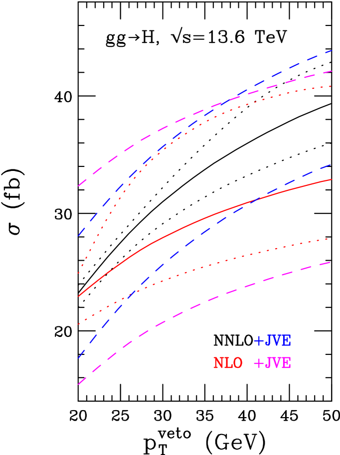
(b) $H$ production.

Figure 3: Comparison of NLO and fixed order predictions as a function of the jet veto. Central predictions solid, uncertainty estimates using either the two-scale approach (dotted) or the envelope of that and the JVE approach (dashed).

Predictions for $WW$ and $ZZ$ production (with $\mu_{h}=Q$) are shown in Fig. 4. The limited overlap between the NLO and bands indicates that uncertainties are underestimated, even with the generous scale uncertainty procedure that we follow. The additional uncertainty resulting from the JVE procedure is small, especially at , because the scale uncertainty of the inclusive cross-sections is very small.

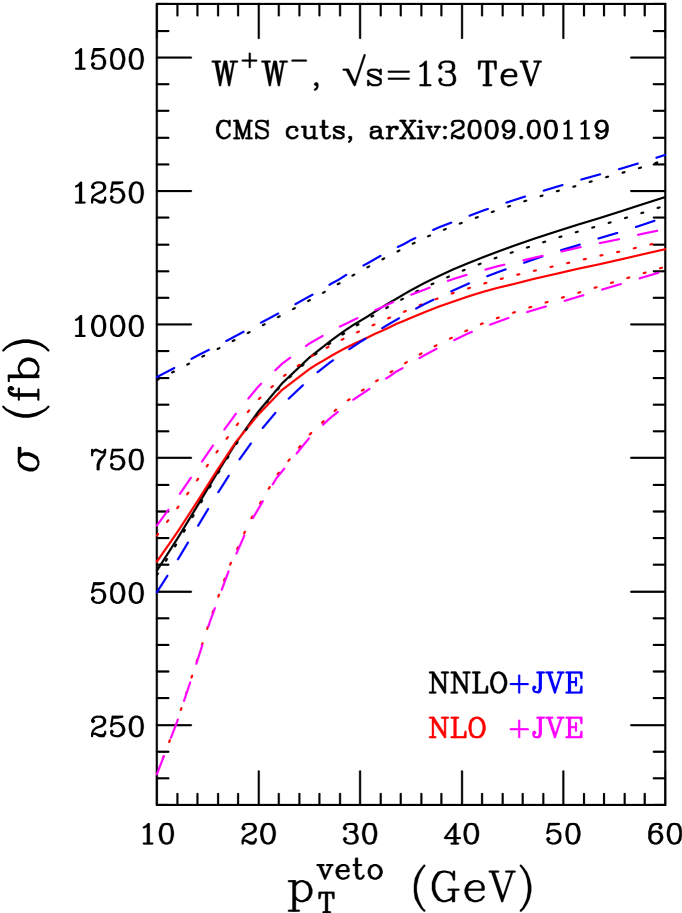
(a) $WW$ production using the setup of ref. CMS:2020mxy .

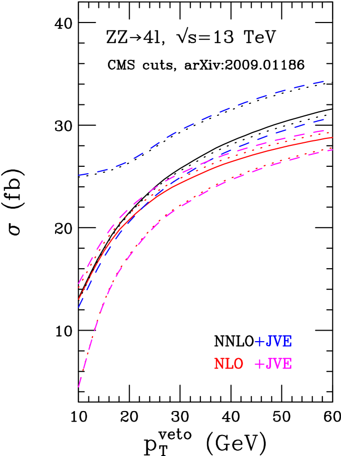
(b) $ZZ$ production using the setup of ref. CMS:2020gtj .

Figure 4: Comparison of NLO and fixed order predictions as a function of the jet veto. Central predictions solid, uncertainty estimates using either the two-scale approach (dotted) or the envelope of that and the JVE approach (dashed).

3.3 Uncertainty estimates at the resummed and matched level

For our central predictions, we set the resummation and factorization scales to $\mu=p_{T}^{\rm veto}$ and the hard scale (corresponding to the renormalization scale) to $\mu_{h}=Q$, where $Q$ is the invariant mass of the color-singlet final state. The exception is Higgs production, where we choose $\mu_{h}=Q/2$ as previously discussed. For the collinear anomaly coefficient $d_{3}^{{\rm veto}}$, we use the form given in Eq. 24 Banfi:2015pju with $R_{0}=1$.

Complications arising at fixed order, described in Section 3.2, are not present in the resummed case and therefore we can follow a simpler approach where we vary all scales in our formalism and take the envelope, as detailed below. While the matching of resummed predictions to fixed-order could still introduce a complication, the matching corrections are not dominant. The bulk of the cross-section comes from the resummation and it allows us to follow the simple procedure of varying all scales in the naively obtained (without JVE) jet-veto cross-section too.

The small and narrowing uncertainty bands at fixed order would typically appear in regions where the resummation is found to be dominant, i.e. where fixed-order contributes very little through the matching corrections. In practice we observe that the size of uncertainties are overall uniform in both the resummation and large $p_{T}^{\rm veto}$ fixed-order regions, as can be seen in all of our following predictions. This supports the conclusion that our procedure is sufficient.

Overall, our procedure for estimating uncertainties is as follows.

1. For the resummation (fixed-order) parts we vary both the resummation (factorization) and hard (renormalization) scales by a factor of two about their central values, adding the excursions in quadrature to obtain the total scale uncertainty.

2. For the resummation we re-introduce the rapidity scale in Eq. (5) by re-writing the collinear anomaly factor as follows Becher:2013xia ; Jaiswal:2015nka :

   $$\bigg{(}\frac{Q}{p_{T}^{\rm veto}}\bigg{)}^{-2F_{ii}(p_{T}^{\rm veto},R,\mu)}=\bigg{(}\frac{Q}{\nu}\bigg{)}^{-2F_{ii}(p_{T}^{\rm veto},R,\mu)}\bigg{(}\frac{\nu}{p_{T}^{\rm veto}}\bigg{)}^{-2F_{ii}(p_{T}^{\rm veto},R,\mu)}\,.$$ (27)

   For $\nu\sim p_{T}^{\rm veto}$ the second factor can be expanded since it does not contain a large logarithm. We vary the rapidity scale $\nu$ in the range $[p_{T}^{\rm veto}/2,2p_{T}^{\rm veto}]$ for gluon-initiated processes and in the range $[p_{T}^{\rm veto}/6,6p_{T}^{\rm veto}]$ for quark-initiated processes. The large variation for quark-initiated processes ensures overlapping uncertainty bands at NNLL and N³LL${}_{\text{p}}$; this is achieved by the range given above, as demonstrated explicitly in Sections 4 and 5.

3. The parameter $R_{0}$ in $d_{3}^{{\rm veto}}$ is varied between $0.5$ and 2.

We first combine the scale uncertainties (1 and 2) in quadrature and then, to obtain our total uncertainty, add the variation of $R_{0}$ (3) linearly.

3.4 Effects of cuts on rapidity at fixed order

The usual jet veto resummation described so far imposes no cut on the jet rapidity. This is in contrast to experimental analyses, see Table 3, which impose such a cut because of limited detector acceptance and to diminish the effect of pileup. Ref. Michel:2018hui identifies three different regimes, depending on $p_{t},Q$ and $y_{\text{cut}}$.

• For $p_{T}^{\rm veto}/Q\gg\exp(-y_{\text{cut}})$ standard jet veto resummation should apply, effects due to the rapidity cut are corrections power suppressed by $Q\exp(-y_{\text{cut}})/p_{T}^{\rm veto}$.

• For $p_{T}^{\rm veto}/Q\sim\exp(-y_{\text{cut}})$ the effects of a rapidity cut must be treated as a leading power correction.

• For $p_{T}^{\rm veto}/Q\ll\exp(-y_{\text{cut}})$ the logarithmic structure is changed already at leading log level, and non-global logarithms appear.

Table 3: Jet rapidity cuts applied in the experimental studies examined later in this paper.

Process	Ref.	$y_{\text{cut}}$
Higgs	–	no study
$Z$ (CMS)	CMS:2022ilp	$2.4$
$W$ (ATLAS)	ATLAS:2017irc	$4.4$
$WW$ (CMS)	CMS:2020mxy	$4.5$
$WZ$ (ATLAS)	ATLAS:2019bsc	$4.5$
$WZ$ (CMS)	CMS:2021icx	$2.5$
$ZZ$ (CMS)	–	no study

We estimate the practical impact of experimentally used jet rapidity cuts at fixed order. Including the rapidity cut in the resummation requires large changes and ingredients, which are also only available a low order so far Michel:2018hui .

The effect of the jet rapidity cut for the $Z$ and Higgs production cases is illustrated in Fig. 5. These calculations are performed at for $p_{T}^{\rm veto}=30$ GeV. The rapidity cut plays a bigger role for Higgs production: for example for $y_{\text{cut}}=2.5$ the cross-section is 11% larger than the result with no rapidity cut, compared to only 2% for $Z$ production. This is due to the larger logarithm ($\log(m_{H}/p_{T}^{\rm veto})/\log(m_{Z}/p_{T}^{\rm veto})\approx 1.28$) and the larger color prefactor ($C_{A}/C_{F}$ = 2.25) in Higgs production. However, for $y_{\text{cut}}=4.5$ the effect of the rapidity cut is negligible in both cases.

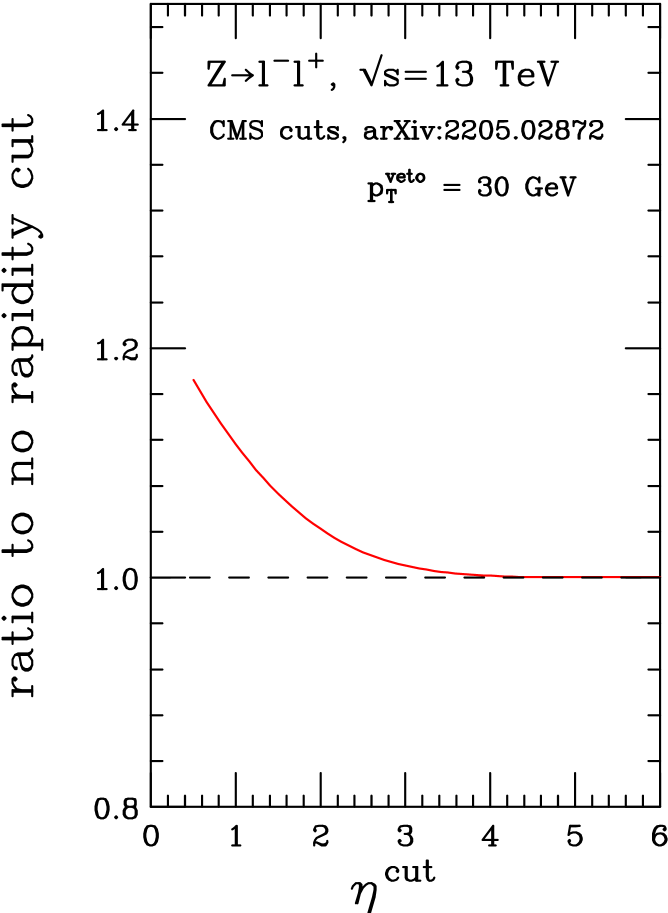
(a) $Z$ production following the setup of ref. CMS:2022ilp .

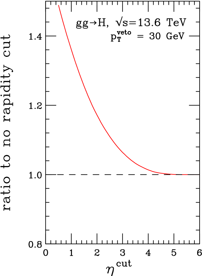
(b) $H$ production.

Figure 5: Effect of the jet rapidity cut at with $p_{T}^{\rm veto}=30$ GeV.

The corresponding results for diboson processes are shown in Fig. 6. In this case, the disparity between $Q$ and $p_{T}^{\rm veto}$ is much larger, so the rapidity cut can play a crucial role, although the effect is still not as important as for Higgs production. For $y_{\text{cut}}=2.5$ the $WW$ and $ZZ$ cross-sections 4% larger than the results with no rapidity cut, and the effect of $y_{\text{cut}}=4.5$ is negligible.

(a) $WW$ production.

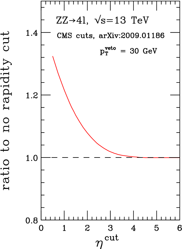
(b) $ZZ$ production.

Figure 6: Effect of the jet rapidity cut at with $p_{T}^{\rm veto}=30$ GeV.

4 Comparison with JetVHeto

While jet-veto resummed phenomenology has been extensively studied in the literature, the only public codes that permit detailed predictions use JetVHeto or RadISH. For jet-veto resummation RadISH implements the analytic JetVHeto resummation formula Banfi:2012jm . The codes rely on the formalism of the CAESAR approach Banfi:2004yd ; Banfi:2012yh extended to NNLL Banfi:2012jm . An extension of the RadISH code has been used to perform joint jet-veto and boson transverse momentum resummation Monni:2019yyr .

For our comparisons we use RadISH version 3.0.0 Bizon:2017rah ; Monni:2016ktx and JetVHeto version 3.0.0 Banfi:2015pju ; Banfi:2012jm ; Banfi:2013eda including small-$R$ resummation Dasgupta:2014yra ; Banfi:2012yh as part of MCFM-RE Arpino:2019fmo . Both codes operate at the level of NNLL and we have checked that they give indeed the same results.

In our comparison, we would like focus on the differences in the resummation part, since the fixed-order part is identical in each calculation. We explore how central values and uncertainties compare at NNLL to our results and in how far N³LL${}_{\text{p}}$ results improve the perturbative convergence. However, the matching to fixed-order is handled differently in each formalism. Different matching schemes (e.g. additive or multiplicative schemes of various types) probe higher-order effects. It has also been advocated to match at the level of jet-veto efficiencies Banfi:2015pju . Fortunately, matching corrections are generally small for jet-veto scales of $3040\text{\,}\mathrm{GeV}$ for all considered boson and di-boson processes. We therefore focus on the resummation in our comparison.

The JetVHeto formalism considers three scales $\mu_{R}$, $\mu_{F}$ and $Q$ that are all similar in magnitude to the hard scale. To ensure that the resummation switches off for $p_{T}^{\rm veto}{}\gtrsim Q$, the resummed logarithms are modified through the prescription $\log(Q/p_{T}^{\rm veto}{})\to 1/p\,\log((Q/p_{T}^{\rm veto}{})^{p}+1)$. For JetVHeto $p$ has a default value of $5$ Banfi:2015pju , while for RadISH the default choice is $4$. For comparison purposes we use $p=5$ in both cases. It is evident that for sufficiently small $p_{T}^{\rm veto}{}$ the precise value of $p$ does not matter. Changing this parameter has a similar effect to turning off the resummation with a transition function. In principle this demands a fully matched calculation, but the matching corrections of our considered cases are small and we have checked that the effect of changing $p$ to $3$ or $4$ is subleading compared to the scale uncertainties. Here we focus on those scale uncertainties.

In ref. Banfi:2015pju it has been argued that the $Q$ should be varied by a factor of $\frac{3}{2}$ around its central value, based on new insights from convergence at N³LO for Higgs production. For simplicity, we use a more conservative variation by a factor of two. We independently vary $\mu_{R},\mu_{F}$ and $Q$ by a factor of two around a central scale of $m_{\ell\ell}$ for $Z$-boson production and around $m_{H}/2$ for Higgs production. Our uncertainty bands for this comparison are obtained by taking the envelope of these results.

$Z$-boson production

For the comparison of $Z$ production we choose a central hard scale of $m_{\ell\ell}$ with results shown in Fig. 7. We find that the uncertainty bands of our MCFM NNLL predictions mostly contain those obtained by JetVHeto (as estimated according to our procedure just described). Furthermore, the uncertainty bands of both NNLL predictions overlap with our N³LL${}_{\text{p}}$ results, indicating robust uncertainties.

At N³LL${}_{\text{p}}$ uncertainties decrease dramatically compared to NNLL, but they are quite asymmetric, which suggests that a symmetrization of uncertainties may be necessary in this case. We also observe that without the large uncertainties at NNLL, there would be no overlap between the N³LL${}_{\text{p}}$ results and NNLL. This highlights the importance of carefully estimating and comparing uncertainties to accurately assess the compatibility of different methods and results.

Figure 7: Comparison of JetVHeto NNLL resummation with our NNLL and N³LL${}_{\text{p}}$ results for $Z$ production with cuts as in Table 4.

$H$-boson production

In our study of Higgs production, we choose a central hard scale of $m_{H}/2$ and show results in Fig. 8. All results are computed in the $m_{t}\to\infty$ theory and rescaled by a factor of $1.0653$ to account for finite top-quark mass effects, see Eq. 144.

The Higgs case is distinct from $Z$ production since it is gluon-gluon initiated instead of quark-initiated. In this case, our predictions agree well with the JetVHeto results, but our uncertainties at NNLL are again much larger.

Note that we vary the JetVHeto scale $Q$ by a factor of two, while the JetVHeto authors vary by a factor of $3/2$ in the Higgs case. This difference in the amount of variation may require some tuning in our formalism, at least at the NNLL level. However, the perturbative convergence is again excellent with small uncertainties at N³LL${}_{\text{p}}$ and central predictions that agree well with NNLL.

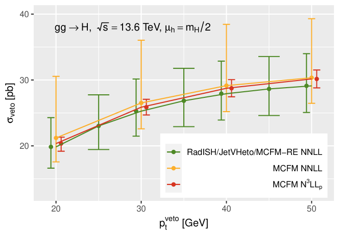
Figure 8: Comparison of JetVHeto NNLL resummation with our NNLL and N³LL${}_{\text{p}}$ results for non-decaying $H$ production.

5 Phenomenological results

In this section, we present the results of our phenomenological studies, which are based on the uncertainty procedure, matching to fixed-order, and input parameters described in Section 3. We compare our findings with experimental results from the literature and discuss their implications.

5.1 $Z$ and $W$ production

The process of $Z$ production has already been extensively studied in the literature, thus enabling a variety of cross-checks of our calculation. The implementation of the hard function and its evolution has been verified by comparison with the explicit results given in Table 1 of ref. Becher:2011xn . The full machinery of the resummation and matching procedure can also be compared with the results of ref. Banfi:2012jm , with which we find excellent agreement within uncertainties, see also Section 4.

We first investigate the impact of choosing a time-like hard scale in the resummed result for $Z$ production. Previous work has shown that choosing a space-like hard scale ($\mu_{h}^{2}=Q^{2}$) can lead to significant corrections in the perturbative expansion of some processes, while a time-like hard scale ($\mu_{h}^{2}=-Q^{2}$) can resum certain $\pi^{2}$ contributions Ahrens:2008qu using a complex strong coupling.

Table 4: Cuts used in the analysis of $Z$ production, adapted from ref. CMS:2022ilp .

lepton cuts	$q_{T}^{l_{1}}>$30\text{\,}\mathrm{GeV}$$, $q_{T}^{l_{2}}>$20\text{\,}\mathrm{GeV}$$, $|\eta^{l}|<2.4$
lepton pair mass	$$71\text{\,}\mathrm{GeV}$<m_{l^{-}l^{+}}<$111\text{\,}\mathrm{GeV}$$
jet veto	anti-$k_{T}$, $R=0.4$, 0-jet events only

For this comparison we consider purely resummed results at NNLL and N³LL${}_{\text{p}}$, only considering uncertainties originating from scale variation (items 1 and 2 of our uncertainty procedure in Section 3.3). We consider the process $pp\to Z/\gamma^{*}\to\ell^{-}\ell^{+}$, i.e. a final state of definite lepton flavor. We use the same set of cuts and vetoes as in the $\sqrt{s}=$13\text{\,}\mathrm{TeV}$$ CMS analysis CMS:2022ilp , but extend the veto to jets of all rapidities, rather than only those with $|y|<2.4$. This difference, and the effect of matching to , is discussed in detail in Section 5.1.1.

Our results are shown in Fig. 9(a) as a function of the value of the jet veto. We observe that the results do not depend strongly on the choice of hard scale, with a difference of about $4\%$ at NNLL and only $1\%$ at N³LL${}_{\text{p}}$. This indicates that resumming the $\pi^{2}$ terms results in only a small enhancement of the cross-section for $W$ and $Z$ production. Based on these findings, we use the space-like hard scale ($\mu_{h}^{2}=Q^{2}$) in our subsequent studies of $Z$ and $W$ boson production, as it is the more commonly used choice in the literature.

(a) Predictions are computed using a central choice for the hard scale given by either $\mu_{h}^{2}=Q^{2}$ or $\mu_{h}^{2}=-Q^{2}$. The lower panel shows the ratio of the result for $\mu_{h}^{2}=-Q^{2}$ to the one for $\mu_{h}^{2}=Q^{2}$.

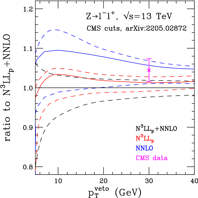
(b) Predictions and CMS measurement as ratio to matched result.

Figure 9: Comparison of NNLL and N³LL${}_{\text{p}}$ predictions for $Z$ production as a function of the jet veto, using the setup of ref. CMS:2022ilp (central predictions solid, uncertainty estimate according to the text, dashed).

5.1.1 CMS $Z$ production

As previously mentioned, the CMS measurement we are comparing to includes a jet rapidity cut of $|y|<2.4$. To assess the importance of this restriction, we first compare the predictions with and without the rapidity cut, as a function of the jet veto value. This comparison, shown in Table 5, helps us better understand the limitations of our analysis.

We use the quantity $\epsilon(p_{T}^{\text{veto}})$ to quantify the increase in the cross-section when the rapidity cut is applied, defined as

$$\epsilon(p_{T}^{\text{veto}})=\frac{\sigma_{0-\text{jet}}(y_{\text{cut}}=2.4)}{\sigma_{0-\text{jet}}(\text{no}~{}y_{\text{cut}})}-1\,.$$ (28)

The experimental measurement we are comparing to uses a jet veto of $p_{T}^{\text{veto}}=$30\text{\,}\mathrm{GeV}$$, for which the rapidity cut has only a 3% effect on the cross-section. This suggests that our calculation with an all-rapidity jet veto is appropriate for comparing to the experimental measurement. However, as $p_{T}^{\text{veto}}$ decreases, the impact of the rapidity cut becomes more significant, until at $p_{T}^{\text{veto}}=$5\text{\,}\mathrm{GeV}$$ it is no longer appropriate to neglect the rapidity cut. This is consistent with the arguments of Ref. Michel:2018hui , which suggest that the standard jet veto resummation formalism should suffice as long as $\ln(Q/p_{T}^{\text{veto}})\ll y_{\text{cut}}$. In our case, $\ln(Q/p_{T}^{\text{veto}})$ ranges from 0.8 to 2.9 for $p_{T}^{\text{veto}}$ from 40 down to $5$ GeV, so the standard jet veto resummation should be appropriate, albeit with sizeable power corrections, for $y_{\text{cut}}=2.4$ except for the smallest values of $p_{T}^{\rm veto}$.

Table 5: The $Z+0$-jet cross-section prediction at NNLO ($\mu=Q$), with and without a jet rapidity cut.

$p_{T}^{\text{veto}}$ [GeV]	5	10	20	30	40
$\sigma_{0-\text{jet}}(\text{no}~{}y_{\text{cut}})$ [pb]	140	347	539	627	675
$\sigma_{0-\text{jet}}(y_{\text{cut}}=2.4)$ [pb]	242	411	569	643	685
$\epsilon$	0.73	0.18	0.06	0.03	0.01

We now turn to a comparison with the CMS result CMS:2022ilp , which uses a jet threshold of $30$ GeV. Our comparison with fixed-order, purely resummed and matched predictions is shown in Fig. 10. We find that the fixed-order and resummed results differ by only a few percent, indicating that resummation is not necessary for this value of the jet veto. This is because the quantity $\ln(M_{Z}/p_{T}^{\rm veto})=1.1$ is not large enough to require resummation. The CMS measurement yields a cross-section of $618\pm 17\text{\,}\mathrm{p}\mathrm{b}$, while our best prediction is $592^{+11}_{-14}\,$pb.

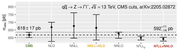
Figure 10: Comparison of $Z$-boson jet-vetoed predictions with the CMS CMS:2022ilp $13\text{\,}\mathrm{TeV}$ measurement. Shown are results at fixed-order, purely resummed and matched.

We study the production of $Z$ bosons as a function of the jet veto in Fig. 9(b). We observe that the difference between the resummed and central fixed-order results is small, even for the smallest values of $p_{T}^{\rm veto}$ considered. However, the uncertainties in the fixed-order prediction are larger across the whole range, particularly for small $p_{T}^{\rm veto}$. For values of $p_{T}^{\rm veto}$ in the range of $2040\text{\,}\mathrm{GeV}$, which are of practical interest, the N³LL${}_{\text{p}}$ uncertainty is smaller than the uncertainty by about a factor of 1.5.

5.1.2 ATLAS $W$ production

We now perform a comparison with $\sqrt{s}=$8\text{\,}\mathrm{TeV}$$ ATLAS data on $W$ production ATLAS:2017irc . For this study, jets were identified using the anti-$k_{T}$ algorithm with $R=0.4$ and must satisfy $p_{T}>30$ GeV and $|y|<4.4$. We have checked at fixed order that this large rapidity cut has a negligible impact of a few per mille, i.e. results are unchanged within the numerical precision to which we work.

Summing over both $W$ charges and including only the decay into electrons we compare our predictions in Fig. 11. We show results at fixed order, at the resummed level, and at the matched level. The effect of matching is large and we thus conclude that this value for the jet veto is outside the sensible range for a purely resummed result, unlike for the $Z$ study in the previous subsection.

We observe excellent agreement with the theoretical prediction, albeit with a larger experimental uncertainty. The experimentally measured cross-section is $4.72\pm 0.3\text{\,}\mathrm{n}\mathrm{b}$ while our best prediction is $4.71^{+0.09}_{-0.11}\,$nb. Since this measurement corresponds to an integrated luminosity of only $20\text{\,}\mathrm{f}\mathrm{b}^{-1}$ it is clear that the high-luminosity LHC will eventually be able to provide a much keener test of perturbative QCD in this process.

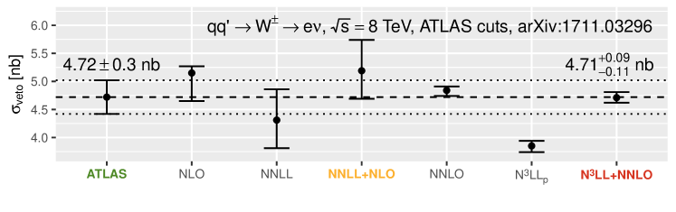
Figure 11: Comparison of $W$-boson jet-vetoed predictions with the ATLAS ATLAS:2017irc $8\text{\,}\mathrm{TeV}$ measurement. Shown are results at fixed-order, purely resummed and matched.

5.2 $W^{+}W^{-}$ production

Experimental studies of $WW$ production were performed by both ATLAS ATLAS:2017bbg ; ATLAS:2019rob and CMS CMS:2019ppl ; CMS:2020mxy . Here we focus on the CMS analysis of ref. CMS:2020mxy since it provides a measurement of the $0$-jet cross-section as a function of the jet $p_{T}$ veto. This cross-section measurment corresponds to a sum over both electron and muon decays of the $W$ bosons, which we denote by the label $pp\to W^{-}W^{+}\to 2\ell 2\nu$. In order to account for this in our calculation, we compute the result for $pp\to e^{-}\mu^{+}\bar{\nu}_{e}\nu_{\mu}$ at and multiply it by the factor that accounts exactly for all lepton combinations through NLO. The impact of $ZZ$ contributions in the same-flavor case results in a slight enhancement over the naïve factor of four. We find that, independent of the value of the jet veto in the range that we consider, this factor is equal to $4.15$.

The CMS analysis only imposes a jet rapidity cut of $y_{\text{cut}}=4.5$, so our expectation is that the standard jet veto resummation formalism should be appropriate for $p_{T}^{\text{veto}}$ values between 60 and $10$ GeV, since in this case the logarithm of the ratio of $Q$ to $p_{T}^{\text{veto}}$ are in the range of 1.3 to 3.1. This expectation is supported by the analysis in Table 6, which shows only a small 2% effect from the rapidity cut for $p_{T}^{\text{veto}}=10$ GeV (and none for values above that). Unlike the processes considered so far, $Q$ is no longer set by a resonance mass but is instead a distribution with a peak slightly above the $2M_{W}$ threshold. For illustration, we have used an average value of $Q\sim$220\text{\,}\mathrm{GeV}$$.

Table 6: The $pp\to W^{-}W^{+}\to 2\ell 2\nu+$0-jet cross-section at , with and without a jet rapidity cut.

$p_{T}^{\text{veto}}$ [GeV]	10	25	30	35	45	60
$\sigma_{0-\text{jet}}(\text{no}~{}y_{\text{cut}})$ [fb]	535	963	1004	1054	1145	1237
$\sigma_{0-\text{jet}}(y_{\text{cut}}=4.5)$ [fb]	548	963	1004	1054	1145	1237
$\epsilon$	0.02	0.00	0.00	0.00	0.00	0.00

We first fix the value of $p_{T}^{\rm veto}=$30\text{\,}\mathrm{GeV}$$ and study the sensitivity of the pure fixed-order and resummed calculations to the jet-clustering parameter $R$. The results are shown in Fig. 12(a). At NLO, there is at most one additional parton, so the NLO result does not depend on the value of $R$. However, the NNLL result exhibits a mild dependence on $R$, which is most noticeable in the size of the uncertainties. These uncertainties are much larger for smaller values of $R$, as was previously observed and discussed in the context of Higgs production in Ref. Becher:2013xia . At , the fixed-order calculation becomes sensitive to the value of $R$, although the dependence is very small. At N³LL${}_{\text{p}}$, the dependence is reduced compared to NNLL, especially at small $R$. Overall, these results suggest that the jet-clustering parameter has a mild effect on the predictions of the fixed-order and resummed calculations for $WW$ production. We have not investigated the effect of small $R$ resummation Banfi:2015pju on these results.

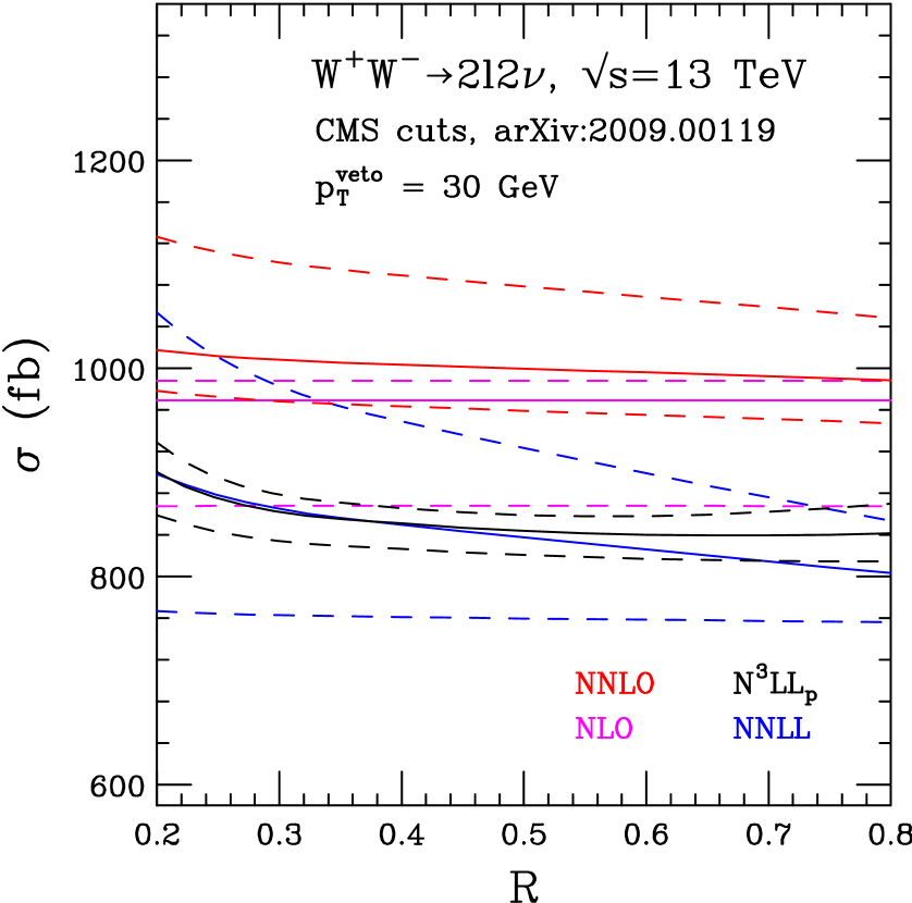
(a) Jet radius $R$ dependence of fixed-order and purely resummed results.

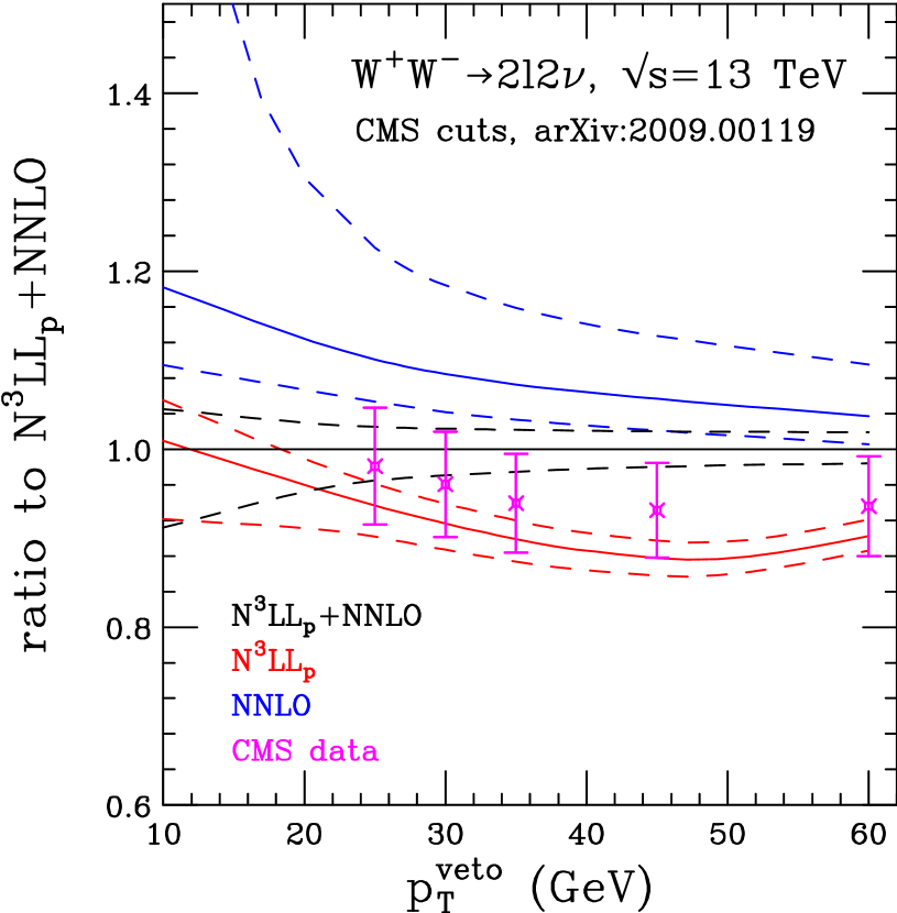
(b) Predictions and CMS measurement as a ratio to the matched result.

Figure 12: Comparison of , N³LL${}_{\text{p}}$ and matched N³LL${}_{\text{p}}$+ results for $W^{+}W^{-}$ production.

In Fig. 12(b), we extend our previous analysis of the jet-veto dependence of $WW$ production, which was presented in Ref. Campbell:2022uzw . The effect of matching is substantial for values of $p_{T}^{\rm veto}$ greater than $20\text{\,}\mathrm{GeV}$, so for typical jet vetoes in the range of $2040\text{\,}\mathrm{GeV}$, matched predictions are important. We find that the fixed-order description is only capable of providing an adequate result for the highest value of $p_{T}^{\rm veto}$ studied here. A comparison with the CMS measurement shows better agreement with the matched resummed calculation, although the experimental uncertainties are still substantial, corresponding to an integrated luminosity of 36 fb^-1. A breakdown of the estimated uncertainty on the matched N³LL${}_{\text{p}}$+ prediction, into the categories described in Section 3.3, is shown in Fig. 13. The uncertainty from the variation of the hard (renormalization) and resummation (factorization) scales dominates, except for the very lowest values of $p_{T}^{\rm veto}$ where the uncertainty on $d_{3}^{{\rm veto}}$ becomes significant.

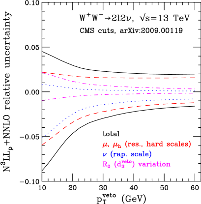
Figure 13: Uncertainty breakdown of the N³LL${}_{\text{p}}$+ results for $W^{+}W^{-}$ production.

We eagerly anticipate a measurement with more statistics in order to hone this comparison. Future measurements with higher precision and larger data samples will provide a more stringent test of the theoretical predictions and help to refine our understanding of $WW$ production at the LHC.

5.3 $W^{\pm}Z$ production

5.3.1 ATLAS

For $W^{\pm}Z$ production, we first compare our results with an analysis from the ATLAS collaboration at $\sqrt{s}=$13\text{\,}\mathrm{TeV}$$ ATLAS:2019bsc . The $0$-jet cross-section is measured with jets defined by the anti-$k_{T}$ algorithm with $p_{T}>25$ GeV, $|y|<4.5$, and $R=0.4$.

Since $\ln(Q/p_{T}^{\text{veto}})=2.3$ (for $p_{T}^{\text{veto}}=$25\text{\,}\mathrm{GeV}$$, using an average $Q$ of about $240\text{\,}\mathrm{GeV}$), we expect that standard jet veto resummation should be applicable in this case, since $y_{\text{cut}}=4.5$. We have checked that the effect of the rapidity cut is at the per mille level, which is less than our numerical precision.

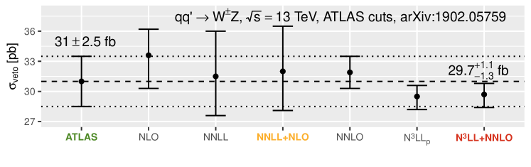
Figure 14: Comparison of $W^{\pm}Z$ jet-vetoed predictions with the ATLAS $13\text{\,}\mathrm{TeV}$ measurement ATLAS:2019bsc . Shown are results at fixed order, purely resummed and matched.

The ATLAS result is presented for a single leptonic channel and summed over both $W$ charges. The corresponding theoretical predictions at fixed order, at the resummed level, and at the matched level are shown in Fig. 14.

Overall, the measurement is in good agreement with both the N³LL${}_{\text{p}}$+ and predictions, within the mutual uncertainties. Only a more precise measurement would be able to definitively support the need for resummation in this case. Since the ATLAS analysis includes only $36\text{\,}\mathrm{f}\mathrm{b}^{-1}$ of data, it is likely that a more precise measurement will be possible in the near future.

5.3.2 CMS

We now contrast the ATLAS study of the $W^{\pm}Z$ process with one from CMS CMS:2021icx . In the CMS study, jets are defined by the anti-$k_{T}$ algorithm with $p_{T}>25$ GeV, $|y|<2.5$, and $R=0.4$.

To assess the applicability of the jet-rapidity inclusive resummation framework, we must compare $\ln(Q/p_{T}^{\text{veto}})=2.3$ with $y_{\text{cut}}=2.5$. This suggests that the standard jet veto resummation formalism may not be appropriate in this case, and that the use of $y_{\text{cut}}$-dependent beam functions Michel:2018hui may be necessary to provide a reliable theoretical prediction. Despite this, we still pursue the comparison here, without using $y_{\text{cut}}$-dependent beam functions, to examine the limitations of our approach.

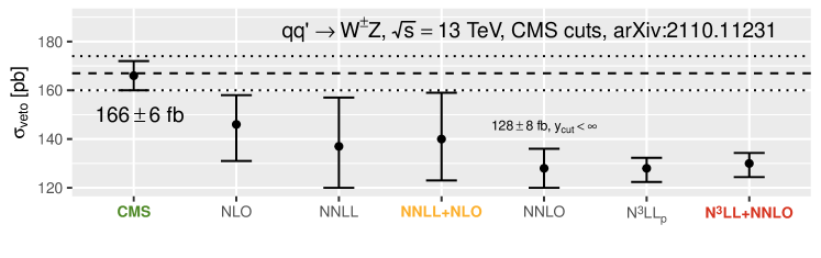
Figure 15: Comparison of $W^{\pm}Z$ jet-vetoed predictions with the CMS CMS:2021icx $13\text{\,}\mathrm{TeV}$ measurement. Shown are results at fixed-order, purely resummed and matched, all without a rapidity cut.

The CMS result for $W^{\pm}Z$ production is presented after summing over all lepton flavors and both $W$ charges. On the theoretical side, we perform a similar analysis, but ignore same-flavor effects that only enter at the 2% level. To construct the jet-vetoed cross-section for the CMS measurement, we combine the differential results in Figure 14(c) of Ref. CMS:2021icx with the inclusive cross-sections reported in Table 6 of the same reference. Our results are shown in Fig. 15.

We find that neither the resummed prediction nor the one are in good agreement with the CMS data, even when the calculation takes the jet rapidity cut into account (increasing the result from $128\text{\,}\mathrm{f}\mathrm{b}$ to $137\text{\,}\mathrm{f}\mathrm{b}$). This suggests that resummation is required in this case, and that the use of $y_{\text{cut}}$-dependent beam functions is necessary to provide a reliable theoretical prediction. Overall, these results highlight the importance of using appropriate resummation techniques to accurately predict $W^{\pm}Z$ production at the LHC with a small jet rapidity cut.

5.4 $ZZ$ production

In the absence of jet-vetoed cross-sections for comparison, we use the cuts from a recent CMS study CMS:2020gtj to investigate our theoretical predictions for $ZZ$ production as a function of $p_{T}^{\rm veto}$. In the results that follow we consider a sum over $Z$ decays into both electrons and muons, which we denote by $pp\to ZZ\to 4$ leptons, and apply the cuts shown in Table 7.

lepton cuts	$q_{T}^{l_{1}}>$20\text{\,}\mathrm{GeV}$$, $q_{T}^{l_{2}}>$10\text{\,}\mathrm{GeV}$$,
	$q_{T}^{l_{3,4}}>$5\text{\,}\mathrm{GeV}$$, $|\eta^{l}|<2.5$
lepton pair mass	$$60\text{\,}\mathrm{GeV}$<m_{l^{-}l^{+}}<$120\text{\,}\mathrm{GeV}$$
jet veto	anti-$k_{T}$, $R=0.5$

Table 7: Fiducial cuts used for the $ZZ$ analysis, taken from the CMS study in Ref. CMS:2020gtj .

We expect that standard jet veto resummation should provide good predictions for $y_{\text{cut}}=4.5$, since $\ln(Q/p_{T}^{\text{veto}})$ is in the range of 1.4 to 3.2 for $p_{T}^{\text{veto}}$ values between 60 and $10\text{\,}\mathrm{GeV}$, using an average $Q$ of about $240\text{\,}\mathrm{GeV}$. For $y_{\text{cut}}=2.5$, we expect larger rapidity effects for the smallest values of $p_{T}^{\text{veto}}$. This is supported by our analysis in Table 8, which shows only a very small (1%) effect from a rapidity cut of $y_{\text{cut}}=4.5$ for $p_{T}^{\text{veto}}=$10\text{\,}\mathrm{GeV}$$ (and no effect for higher values). Even for $y_{\text{cut}}=2.5$, the rapidity cut has a relevant effect only for $p_{T}^{\text{veto}}$ values below $30\text{\,}\mathrm{GeV}$, and is mostly insignificant beyond that.

Table 8: The $ZZ+0$-jet cross-section at ($\mu=Q$), with and without a jet rapidity cut.

$p_{T}^{\text{veto}}$ [GeV]	10	20	30	40	50	60
$\sigma_{0-\text{jet}}(\text{no}~{}y_{\text{cut}})$ [fb]	13.3	21.5	25.8	28.4	30.3	31.6
$\sigma_{0-\text{jet}}(y_{\text{cut}}=4.5)$ [fb]	13.4	21.5	25.8	28.4	30.3	31.6
$\sigma_{0-\text{jet}}(y_{\text{cut}}=2.5)$ [fb]	14.9	22.4	26.3	28.8	30.6	31.8
$\epsilon(y_{\text{cut}}=4.5)$	0.01	0.00	0.00	0.00	0.00	0.00
$\epsilon(y_{\text{cut}}=2.5)$	0.12	0.04	0.02	0.01	0.01	0.01

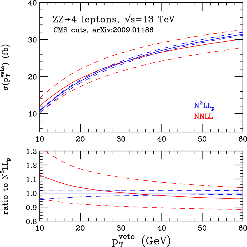
(a) Purely resummed results.

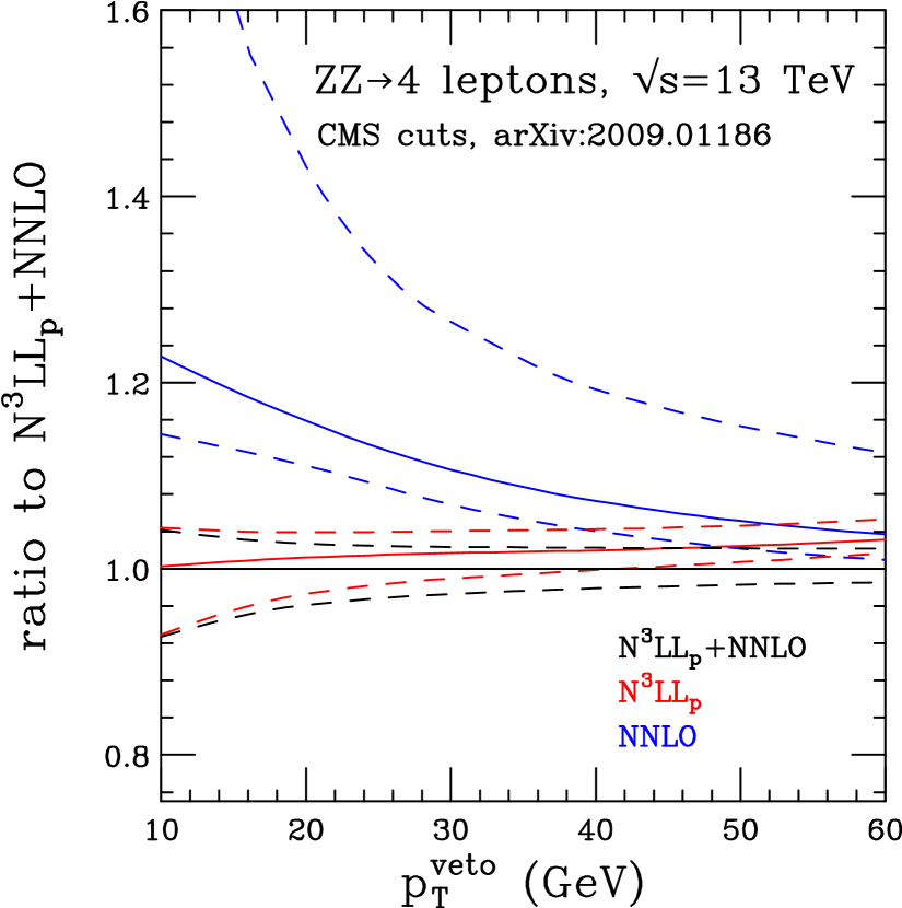
(b) Ratio to matched result.

Figure 16: Comparison of , N³LL${}_{\text{p}}$ and matched N³LL${}_{\text{p}}$+ results for $ZZ$ production as a function of the jet veto.

Fig. 16(a) shows a comparison of the dependence on $p_{T}^{\rm veto}$ for purely-resummed results at two different logarithmic orders. The central predictions are very similar at NNLL and N³LL${}_{\text{p}}$ and are consistent within uncertainties for all values of $p_{T}^{\rm veto}$. Fig. 16(b) compares the matched N³LL${}_{\text{p}}$+ and results. The prediction has large uncertainties over the whole range of $p_{T}^{\rm veto}$ and only overlaps with N³LL${}_{\text{p}}$+ around $40\text{\,}\mathrm{GeV}$ and higher. The difference between the central resummed and fixed-order results is significant (around 10%) for typical values of $p_{T}^{\text{veto}}$ around $30\text{\,}\mathrm{GeV}$. For most relevant values of $p_{T}^{\rm veto}$ at the LHC, resummation is clearly important for providing a precision prediction for this process.

5.5 Higgs production

For gluon fusion Higgs production an important topic is the inclusion of finite top-quark mass effects. Although at these could be included exactly Bonciani:2022jmb ; Czakon:2021yub , the mass effects are not relevant in the jet-vetoed case Neumann:2014nha at the current level of precision. A simple overall one-loop rescaling factor that takes into account the full mass dependence is sufficient to introduce mass effects into $m_{t}\to\infty$ EFT predictions. In the resummation formalism, the coefficient for the matching of Higgs production in QCD onto SCET can be calculated in two ways, referred to as one-step and two-step procedures.

5.5.1 One-step and two-step schemes

The one-step procedure is based on the observation that the ratio $m_{H}/m_{t}$ is not large in a logarithmic sense (c.f. $\rho=m_{H}^{2}/m_{t}^{2}\approx 1/2$ and $\alpha_{s}\log 1/\rho\approx 0.07$). This procedure matches the full QCD result, typically obtained at higher orders as an expansion in the parameter $r$, onto SCET at the scale $\mu_{h}\sim m_{H}$. In this way, terms of order $\rho$ are retained, but logs of $m_{t}/m_{H}$ are neglected.

In the two-step procedure outlined in Refs. Idilbi:2005er ; Idilbi:2005ni ; Ahrens:2009cxz ; Mantry:2009qz , the top quark is first integrated out at a scale $\mu_{t}\approxeq m_{t}$, and then the QCD effective Lagrangian is matched onto the SCET at a scale $\mu_{h}\approxeq m_{H}$. Running between $\mu_{t}$ and $\mu_{h}$ allows one to sum logarithms of $m_{t}/m_{H}$, and finite top-mass effects are included by scaling the result by a correction factor obtained at leading order (an increase with respect to the EFT result by a factor of $1.0653$, see Eq. (144)). Terms enhanced by powers of $m_{H}/m_{t}$ are thus only included in an approximate fashion at NLO and beyond. The one-step procedure is described in detail in Appendix G.1 and the two-step procedure is described in Appendix G.2.

We compare the numerical difference between the one- and two-step schemes, computed at $\sqrt{s}=13.6$ TeV and for $R=0.4$ in Fig. 17(a). Guided by fixed-order results, and in accord with previous studies of this process Banfi:2015pju , we set the hard (renormalization) scale using $\mu_{h}=Q/2$. We observe that the one-step scheme results in a cross-section that is about $1.7$–$2.3\%$ larger at NNLL and only $1.6\%$ larger at N³LL${}_{\text{p}}$. This small difference occurs if one works rigorously at a fixed order of $\alpha_{s}$. Working at a fixed order in $\alpha_{s}$ in the component parts of the two-step scheme can lead to larger differences, as described in more detail in Section G.3.

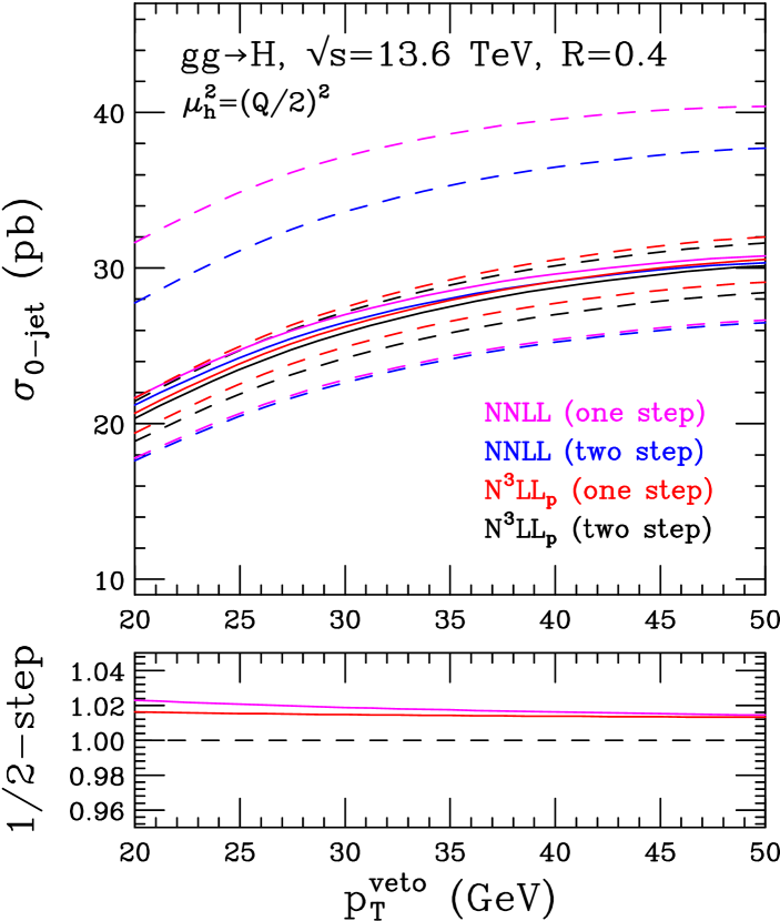
(a) Results in the one- or two-step scheme. The lower panel shows the ratio of the one-step to the two-step result.

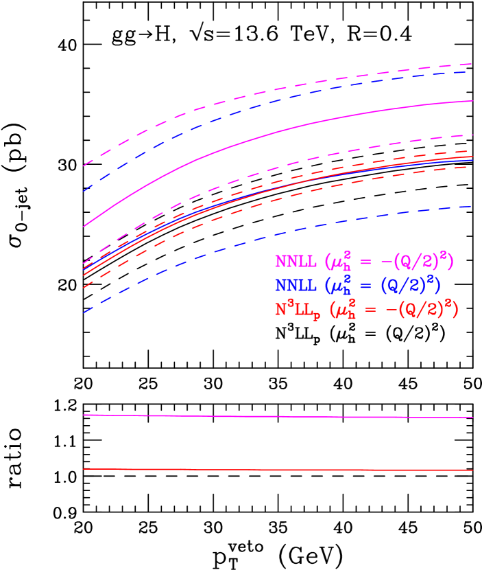
(b) Results using a central scale of either $\mu_{h}^{2}=Q^{2}$ or $\mu_{h}^{2}=-Q^{2}$. The lower panel shows the ratio of the result for $\mu_{h}^{2}=-Q^{2}$ to the one for $\mu_{h}^{2}=Q^{2}$.

Figure 17: Comparison of NNLL and N³LL${}_{\text{p}}$ predictions for Higgs production at $\sqrt{s}=13.6$ TeV as a function of the jet veto.

5.5.2 Time-like vs. space-like $\mu_{h}^{2}$

We now study the impact of choosing a time-like hard scale for the calculation of the Higgs cross-section. To do this, we compare $\mu_{h}^{2}=(Q/2)^{2}$ (the space-like scale) with $\mu_{h}^{2}=-(Q/2)^{2}$ (the time-like scale). The use of a time-like hard scale allows us to resum certain $\pi^{2}$ terms, by employing a complex strong coupling Ahrens:2008qu . For this comparison, we consider purely resummed results at NNLL and N³LL${}_{\text{p}}$ accuracy.

Results are shown in Fig. 17(b), for the two-step scheme computed at $\sqrt{s}=13.6$ TeV with $R=0.4$. We observe that at NNLL, the resummation of the $\pi^{2}$ terms significantly enhances the cross-section by 17%. However, at N³LL${}_{\text{p}}$ accuracy, this resummation only leads to a small increase of 2% in the cross-section.

Results for the matched vetoed cross-section are shown in Fig. 18(a). After matching, we observe substantial agreement between the and N³LL${}_{\text{p}}$+ calculations within uncertainties. The central predictions differ by about 5% across the range, but the uncertainties are substantially smaller in the resummed calculation.

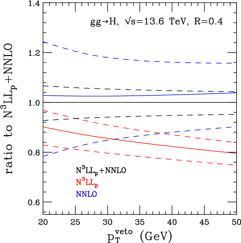
(a) Comparison of NNLL, N³LL${}_{\text{p}}$ and N³LL${}_{\text{p}}$+ predictions.

(b) Uncertainty breakdown of the N³LL${}_{\text{p}}$+ prediction.

Figure 18: Results for Higgs production at $\sqrt{s}=13.6$ TeV as a function of the jet veto.

The estimated uncertainty on the matched N³LL${}_{\text{p}}$+ prediction, broken down into the various sources that we consider, is shown in Fig. 18(b). Although the uncertainty from the variation of $d_{3}^{{\rm veto}}$ reaches 2% for $p_{T}^{\rm veto}=20$ GeV, the uncertainty from the variation of the hard (renormalization) and resummation (factorization) scales dominates across the entire range.

6 Conclusions

We have presented a comprehensive study of jet-veto resummation in the production of color singlet final states using the most up-to-date theoretical ingredients and achieving N³LL${}_{\text{p}}$ accuracy. Our implementation in MCFM improves upon previous public NNLL calculations by reducing theoretical uncertainties, as demonstrated by comparisons with ATLAS and CMS results. Once the one remaining theoretical element, $d_{3}^{{\rm veto}}$, becomes available, it will be simple to upgrade our predictions to full accuracy.

The primary motivation for this work comes from the need for reliable and accurate predictions of jet-veto cross-sections in processes such as Higgs boson and $W^{+}W^{-}$ production, which are commonly used to study new physics at the LHC. In these processes, the imposition of a jet veto is often necessary to suppress backgrounds and enhance sensitivity to new physics signals. Experimental results going beyond these two processes are much less frequent. We encourage the experimental collaborations to consider measurements of more Standard Model processes with a jet veto, as larger data samples become available, to better understand the dependence of these processes on the jet veto parameters $p_{T}^{\rm veto}$ and $R$.

In addition to providing improved predictions for jet-veto cross-sections, our work also serves as a valuable tool for testing and validation of general purpose shower Monte Carlo programs. Our code allows for a detailed investigation of the dependence on the jet parameters $p_{T}^{\rm veto}$ and $R$, providing a benchmark for assessing the logarithmic accuracy and reliability of Monte Carlo simulations in this important class of processes.

Our analysis shows that at the currently experimentally used values of $p_{T}^{\rm veto}$ in $W$ and $Z$ production, the logarithms are not large enough to justify the use of jet-veto resummation. In these cases, fixed-order perturbation theory, which can be used to give the results with a jet veto over a limited range of rapidities, is simpler and sufficient. We have also found that attempts to resum $\pi^{2}$ terms using a timelike renormalization point have little numerical importance at N³LL${}_{\text{p}}$ if the $p_{T}^{\rm veto}$ scale is around $2030\text{\,}\mathrm{GeV}$.

The production of a Higgs boson is an exception among single-boson processes. In this case, the combination of larger corrections from color factors and slightly larger values of the scale ($m_{H}$) appearing in the jet veto logarithms make resummation an important tool for improving the accuracy of predictions. In the appendix we have investigated the differences between the one-step and two-step procedures for calculating the hard function at the scale of $p_{T}^{\rm veto}$. We find agreement within $2\%$ of these two approaches.

The $W^{+}W^{-}$ production process, where the jet veto has experimental importance, requires both resummation and matching to . For the $ZZ$ process resummation is mandatory but the matching to fixed order is less important. Although this reflects the expectation that the resummed prediction is more accurate for systems of higher invariant mass, these findings depend on the exact nature of the cuts for each process. Our work provides a comprehensive theoretical framework for studying jet vetoes in vector boson pair processes, and as data becomes available, a comparative experimental study would be of great interest and could help to validate our theoretical predictions.

Appendix A Reduced beam functions

We have used the two loop beam function in the presence of a jet veto calculated in Ref. Abreu:2022zgo . Their calculation, together with the corresponding soft function Abreu:2022sdc has been performed in SCET using the exponential rapidity regulator Li:2016axz . The beam function for quark initiated processes in the presence of a jet veto has also been presented in Mellin space in Ref. Bell:2022nrj .

The calculation in Ref. Abreu:2022zgo has a perturbative expansion,

$$I_{ij}=\sum_{k=0}^{\infty}\Big{(}\frac{\alpha_{s}}{4\pi}\Big{)}^{k}\,I^{(k)}_{ij}\,.$$ (29)

The beam functions with a jet veto are decomposed into a reference observable, the beam function for the transverse momentum of a color singlet observable and a remainder term accounting for the effects of jet clustering,

$$I_{ij}(x,Q,p_{T}^{\rm veto},R;\mu,\nu)=I^{\perp}_{ij}(x,Q,p_{T}^{\rm veto};\mu,\nu)+\Delta I_{ij}(x,Q,p_{T}^{\rm veto},R;\mu,\nu)\;.$$ (30)

Since the divergence structure of the reference observable is the same as the beam function with a jet veto, $\Delta I_{ij}$ can be calculated in four dimensions. Results for the reference observable are available in Refs. Luo:2019hmp ; Luo:2019bmw .

The reduced beam function kernels $\bar{I}$ as used in our setup are extracted from the coefficient $I$ as

$$\bar{I}_{ij}(z,p_{T}^{\rm veto},R,\mu)=e^{-h^{A}(p_{T}^{\rm veto},\mu)}\,I_{ij}(z,p_{T}^{\rm veto},R,\mu)\,.$$ (31)

They similarly follow a perturbative expansion

$$\bar{I}_{ik}(z,p_{T}^{\rm veto},R,\mu)=\delta_{ik}\,\delta(1-z)+\frac{\alpha_{s}}{4\pi}\bar{I}^{(1)}_{ik}(z,p_{T}^{\rm veto},\mu)+\Big{(}\frac{\alpha_{s}}{4\pi}\Big{)}^{2}\bar{I}^{(2)}_{ik}(z,p_{T}^{\rm veto},R,\mu)+O(\alpha_{s}^{3})\,.$$ (32)

Contributions at order $\alpha_{s}$

The $\alpha_{s}$ contributions to $\bar{I}$ were first obtained in Refs. Becher:2011xn ; Becher:2012qa and read,

$$\bar{I}_{ij}(z,p_{T}^{\rm veto},R,\mu)=\delta(1-z)\,\delta_{ij}+\frac{\alpha_{s}}{4\pi}\left[-2P_{ij}^{(1)}(z)\,L_{\perp}+R^{(1)}_{ij}(z)\right]+{\cal O}(\alpha_{s}^{2})\,,$$ (33)

where $L_{\perp}=2\ln(\mu/p_{T}^{\rm veto})$. $R$ is the jet measure used in Eq. (1) and $R^{(1)}(z)$ is a remainder function given below. At this order there is no dependence on the jet radius, $R$.

Throughout this paper we expand in powers of $\alpha_{s}/(4\pi)$. The one exception to this rule are the perturbative DGLAP splitting functions,

$$P_{ij}(z)=\frac{\alpha_{s}}{2\pi}P^{(1)}(z)+\Big{(}\frac{\alpha_{s}}{2\pi}\Big{)}^{2}P^{(2)}(z)+\ldots$$ (34)

Explicit expressions for $P^{(1)}$ and $P^{(2)}$ are given in Appendices C.2 and C.3. The remainder functions at order $\alpha_{S}$ are Becher:2010tm

$$R^{(1)}_{qq}(z) = C_{F}\left[2(1-z)-\frac{\pi^{2}}{6}\,\delta(1-z)\right],\qquad R^{(1)}_{qg}(z)=4T_{F}\,z(1-z)\,,$$

$$R^{(1)}_{gg}(z) = -C_{A}\,\frac{\pi^{2}}{6}\,\delta(1-z)\,,\qquad R^{(1)}_{gq}(z)=2C_{F}\,z\,.$$ (35)

where $C_{A}=3,C_{F}=\frac{4}{3},T_{F}=\frac{1}{2}$.

Contributions at order $\alpha_{s}^{2}$

At order $\alpha_{s}^{2}$ we have

$$\bar{I}^{(2)}_{ik}(z,p_{T}^{\rm veto},R,\mu)=\big{[}2\*P^{(1)}_{ij}(x)\otimes P^{(1)}_{jk}(y)-\*\beta_{0}\*P^{(1)}_{ik}(z)\big{]}L_{\perp}^{2}$$

$$+\big{[}-4\*P^{(2)}_{ik}(z)+\beta_{0}\*R^{(1)}_{ik}(z)-2\*R^{(1)}_{ij}(x)\otimes P^{(1)}_{jk}(y)\big{]}L_{\perp}+R^{(2)}_{ik}(z,R)\,.$$ (36)

In this equation $\otimes$ represents a convolution,

$$f(x)\otimes g(y)=\int_{0}^{1}\,dx\,\int_{0}^{1}\,dyf(x)\,g(y)\,\delta(z-xy)=\int_{z}^{1}\,\frac{dy}{y}f(z/y)\,g(y)\,.$$ (37)

Explicit expressions for $P^{(1)}$ and $P^{(2)}$ are given in Appendices C.2 and C.3. The expressions for $P^{(1)}\otimes P^{(1)}$, $R^{(1)}\otimes P^{(1)}$ are given in appendix C.4.

The results from Refs. Abreu:2022zgo ; Abreu:2022sdc recast in the language of reduced beam functions allow us to extract $R^{(2)}_{ik}(z,R)$. We have checked that the reduced beam functions have the form predicted by Eqs. 33 and 36. In addition, we have confirmed the known results for the $\alpha_{s}^{2}$ $R$-dependent contribution to the collinear anomaly exponent. The result for the collinear anomaly exponent is given in Section 2.1.

A.1 Structure of the two-loop reduced beam function

While a numerical evaluation of the analytical formulas for the reduced beam functions is possible, we choose to perform a spline interpolation for improved numerical efficiency.

The reduced beam functions contain distributions of the following structure,

$$\bar{I}^{(2)}_{ij}(z,p_{T}^{\rm veto},R,\mu) = \bar{I}^{(2)}_{ij,-1}(p_{T}^{\rm veto},R,\mu)\,\delta(1-z)+\bar{I}^{(2)}_{ij,0}(p_{T}^{\rm veto},R,\mu)\,D_{0}(1-z)$$ (38)

$$+ \bar{I}^{(2)}_{ij,1}(p_{T}^{\rm veto},R,\mu)\,D_{1}(1-z)+\bar{I}^{(2)}_{ij,2}(z,p_{T}^{\rm veto},R,\mu)\,,$$

where,

$$D_{0}(1-z)=\frac{1}{[1-z]_{+}},\;\;\;D_{1}(1-z)=\bigg{[}\frac{\ln(1-z)}{(1-z)}\bigg{]}_{+}\;.$$ (39)

$\bar{I}^{(2)}_{ij,2}(z,p_{T}^{\rm veto},R,\mu)$ contains terms which are regular at $z=1$.

The analytic results for the beam function of Ref. Abreu:2022zgo are presented as a power series in $R$ up to powers of $R^{8}$. The functions themselves contain powers of $1/(1-z)^{n}$, in certain cases up to $n=7$ or $8$. However, these singularities at $z=1$ are fictitious as can be seen by explicit expansion. The beam functions require special treatment in this region for numerical stability.

The dominant region in the convolution of the function $\bar{I}$ with the parton distributions is precisely the region $z\sim 1$. If we assume a parton distribution $f(x)\sim 1/x$ we have,

$$\bar{I}\otimes f=\int_{x}^{1}\frac{dz}{z}\,\bar{I}(z)\,f(x/z)\sim\frac{1}{x}\int_{x}^{1}\,dz\,\bar{I}(z)\,,$$ (40)

showing that all regions of $z$ contribute equally to the integral. However if, as expected, the parton distribution function falls off more rapidly as $x\to 1$, say $f(x)\sim(1-x)^{n}/x$,

$$\bar{I}\otimes f=\int_{x}^{1}\,\frac{dz}{z}\,\bar{I}(z)\,f(x/z)\sim\frac{1}{x}\,\int_{x}^{1}\,dz\,\bar{I}(z)\,(1-x/z)^{n}\,.$$ (41)

Thus, it is precisely the large values of $z$ which are crucial for the integral. In other words, the parton shower process is dominated by cascade from nearby values of $x$. Larger cascades from more distant points are suppressed by the fall-off of the parton distributions. In view of the importance of the region $z=1$, for numerical stability we perform an expansion about $z=1$.

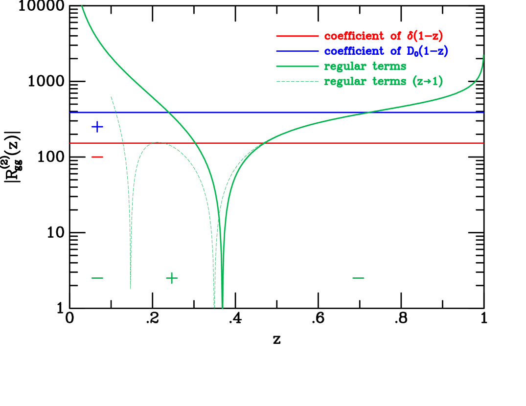
(a) $gg$ case.

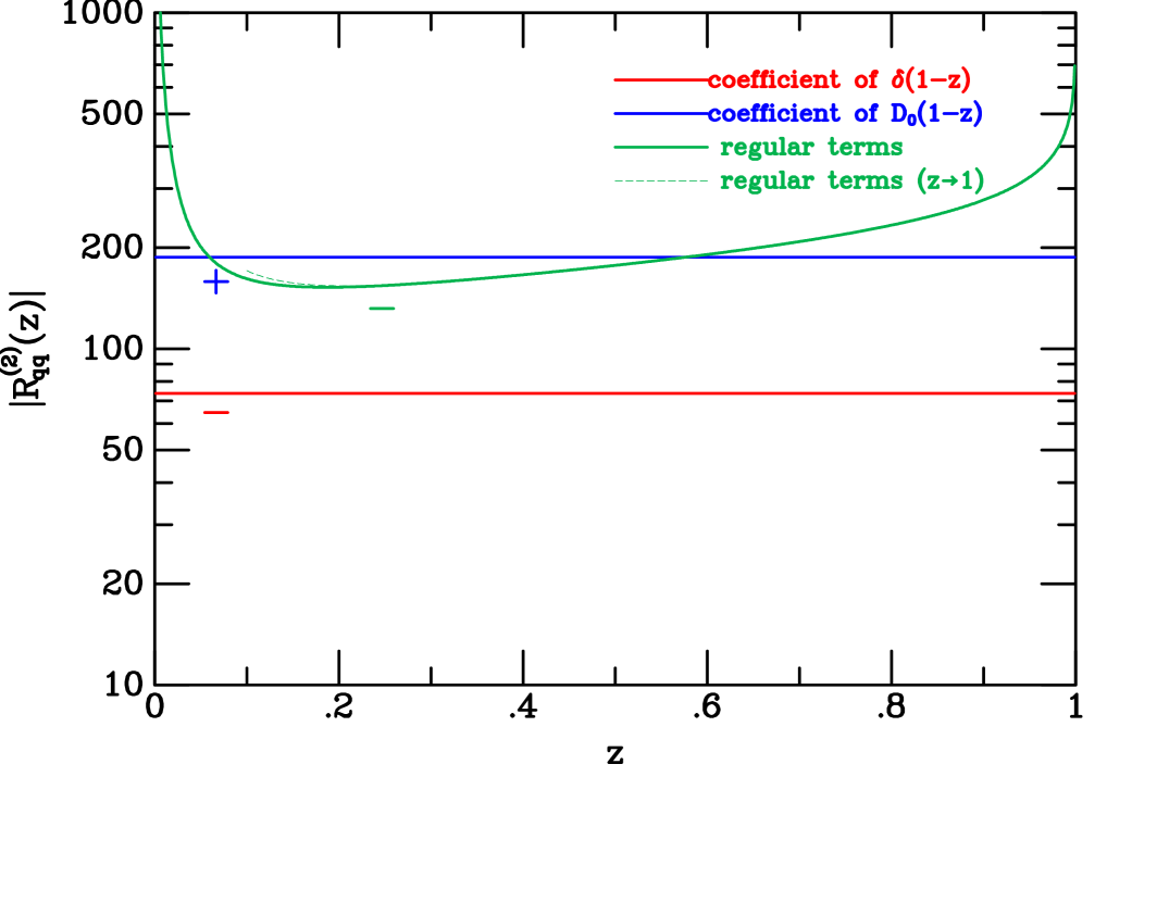
(b) $qq$ case

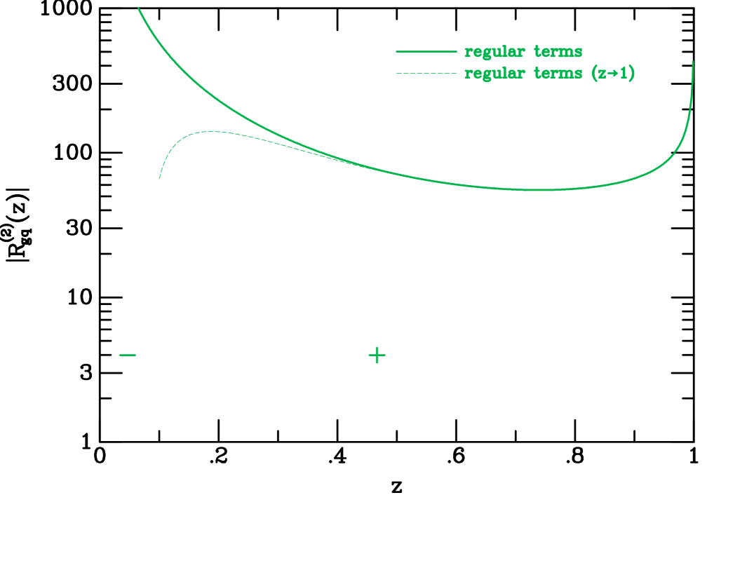
(c) $gq$ case.

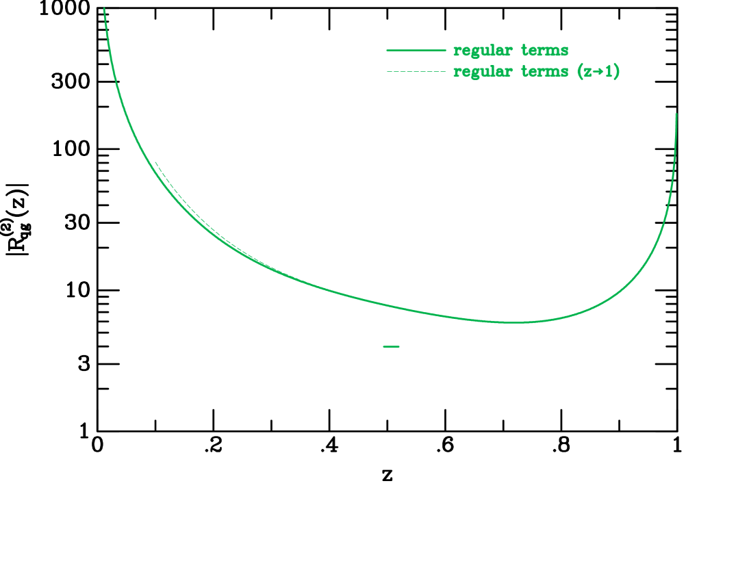
(d) $qg$ case

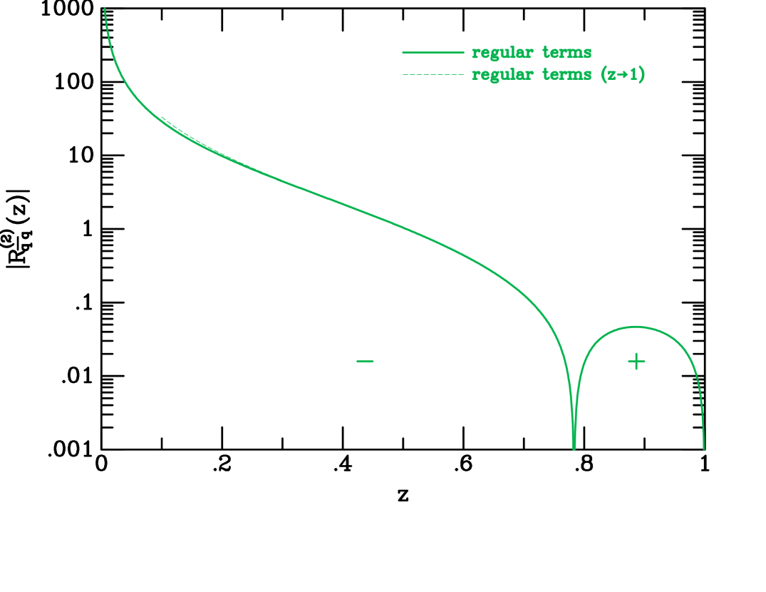
(e) $\bar{q}q$ case.

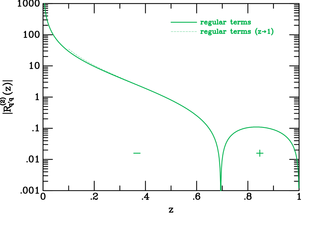
(f) $q^{\prime}q$ case.

Figure 19: Absolute value of $R^{(2)}$ for jet measure $R=0.5$. The $\bar{q}^{\prime}q$ case is the same as the $q^{\prime}q$ case. The sign of the contribution in the various regions is indicated.

The absolute value of $R^{(2)}$ for the various parton transitions is shown in Fig. 19. Individual $R$-dependent terms contain expressions of the form $R^{2n}/(1-z)^{k}$ where $k$ can be a high power. However, the singularity at $z=1$ is only apparent. The resultant limiting forms obtained by series expansion about $z=1$ are shown by the dashed lines in the figures. In practice, we switch to the expanded form at $z=0.9$, although the figures demonstrate that the expanded forms are accurate down to much smaller values of $z$.

Appendix B Definition of the beta function and anomalous dimensions

The coefficients $\beta_{n}$, $\Gamma_{n}^{A}$ and $\gamma_{n}^{g}$ have perturbative expansions in powers of the renormalized coupling. Details are presented below.

B.1 Expansion of $\beta$-function

The beta function is defined as,

$$\frac{d\alpha_{s}(\mu)}{d\ln\mu} = \beta(\mu)=-2\alpha_{s}(\mu)\sum_{n=0}^{\infty}\,\beta_{n}\,\left(\frac{\alpha_{s}}{4\pi}\right)^{n+1}$$ (42)

$$= -2\alpha_{s}(\mu)\,\frac{\alpha_{s}(\mu)}{4\pi}\Big{[}\beta_{0}+\beta_{1}\frac{\alpha_{s}(\mu)}{4\pi}+\beta_{2}\Big{(}\frac{\alpha_{s}(\mu)}{4\pi}\Big{)}^{2}+\beta_{3}\Big{(}\frac{\alpha_{s}(\mu)}{4\pi}\Big{)}^{3}+\ldots\Big{]}\,.$$

The coefficients of the $\overline{\text{MS}}$ $\beta$ function to four loops are Tarasov:1980au ; Larin:1993tp ; vanRitbergen:1997va ,

$$\beta_{0} = \frac{11}{3}\,C_{A}-\frac{4}{3}\,T_{F}\,n_{f}\,,$$

$$\beta_{1} = \frac{34}{3}\,C_{A}^{2}-\Bigl{(}\frac{20}{3}\,C_{A}\,+4C_{F}\Bigr{)}\,T_{F}\,n_{f}\,,$$

$$\beta_{2} = \frac{2857}{54}\,C_{A}^{3}+\Bigl{(}C_{F}^{2}-\frac{205}{18}\,C_{F}C_{A}-\frac{1415}{54}\,C_{A}^{2}\Bigr{)}\,2T_{F}\,n_{f}+\Bigl{(}\frac{11}{9}\,C_{F}+\frac{79}{54}\,C_{A}\Bigr{)}\,4T_{F}^{2}\,n_{f}^{2}\,,$$

$$\beta_{3} = C_{A}^{4}\left(\frac{150653}{486}-\frac{44}{9}\zeta_{3}\right)+C_{A}^{3}T_{F}n_{f}\left(-\frac{39143}{81}+\frac{136}{3}\zeta_{3}\right)$$ (43)

$$+C_{A}^{2}C_{F}T_{F}n_{f}\left(\frac{7073}{243}-\frac{656}{9}\zeta_{3}\right)+C_{A}C_{F}^{2}T_{F}n_{f}\left(-\frac{4204}{27}+\frac{352}{9}\zeta_{3}\right)$$

$$+46C_{F}^{3}T_{F}n_{f}+C_{A}^{2}T_{F}^{2}n_{f}^{2}\left(\frac{7930}{81}+\frac{224}{9}\zeta_{3}\right)+C_{F}^{2}T_{F}^{2}n_{f}^{2}\left(\frac{1352}{27}-\frac{704}{9}\zeta_{3}\right)$$

$$+C_{A}C_{F}T_{F}^{2}n_{f}^{2}\left(\frac{17152}{243}+\frac{448}{9}\zeta_{3}\right)+\frac{424}{243}C_{A}T_{F}^{3}n_{f}^{3}+\frac{1232}{243}C_{F}T_{F}^{3}n_{f}^{3}$$

$$+\frac{d_{A}^{abcd}d_{A}^{abcd}}{N_{A}}\left(-\frac{80}{9}+\frac{704}{3}\zeta_{3}\right)+n_{f}\frac{d_{F}^{abcd}d_{A}^{abcd}}{N_{A}}\left(\frac{512}{9}-\frac{1664}{3}\zeta_{3}\right)$$

$$+n_{f}^{2}\frac{d_{F}^{abcd}d_{F}^{abcd}}{N_{A}}\left(-\frac{704}{9}+\frac{512}{3}\zeta_{3}\right)\,.$$

For the normalization of the $SU(N)$ generators, the conventions of Refs. vanRitbergen:1997va ; vanRitbergen:1998pn are,

$$\frac{d_{A}^{abcd}d_{A}^{abcd}}{N_{A}} = \frac{N^{2}(N^{2}+36)}{24}\,,\quad\frac{d_{F}^{abcd}d_{A}^{abcd}}{N_{A}}=\frac{N(N^{2}+6)}{48}\,,\quad\frac{d_{F}^{abcd}d_{F}^{abcd}}{N_{A}}=\frac{N^{4}-6N^{2}+18}{96N^{2}}\,,$$

$$N_{A} = N^{2}-1\,,\quad N_{F}=N.$$ (44)

Numerical values for the $\beta$-function coefficients are,

$$\beta_{0} = 11-\frac{2}{3}\,n_{f}\,,$$

$$\beta_{1} = 102-\frac{38}{3}\,n_{f}\,,$$

$$\beta_{2} = \frac{2857}{2}-\frac{5033}{18}\,n_{f}+\frac{325}{54}\,n_{f}^{2}\,,$$

$$\beta_{3} = \frac{149753}{6}+3564\zeta_{3}-\Big{(}\frac{1078361}{162}+\frac{6508}{27}\zeta_{3}\Big{)}\,n_{f}+\Big{(}\frac{50065}{162}+\frac{6472}{81}\zeta_{3}\Big{)}\,n_{f}^{2}$$ (45)

$$+ \frac{1093}{729}\,n_{f}^{3}\,.$$

B.2 Cusp Anomalous Dimension

The cusp anomalous dimension depends on the label $B$ which takes the two values, $B=A,F$ for gluons and quarks, respectively. Its perturbative expansion is,

$$\Gamma_{\rm cusp}^{B}(\mu)=\sum_{n=0}^{\infty}\,\Gamma_{n}^{B}\,\left(\frac{\alpha_{s}}{4\pi}\right)^{n+1}\,.$$ (46)

The coefficients up to four loops are Henn:2019swt ; vonManteuffel:2020vjv ,

$$\Gamma^{B}_{0} =4C_{B}\,,$$ (47)

$$\Gamma^{B}_{1} =16C_{B}\bigg{\{}(C_{A}\left(\frac{67}{36}-\frac{\pi^{2}}{12}\right)-\frac{5}{9}n_{f}T_{F}\bigg{\}}\,,$$ (48)

$$\Gamma^{B}_{2} =64C_{B}\bigg{\{}C_{A}^{2}\left(\frac{11\zeta_{3}}{24}+\frac{245}{96}-\frac{67\pi^{2}}{216}+\frac{11\pi^{4}}{720}\right)+n_{f}T_{F}C_{F}\left(\zeta_{3}-\frac{55}{48}\right)$$

$$+n_{f}T_{F}C_{A}\left(-\frac{7\zeta_{3}}{6}-\frac{209}{216}+\frac{5\pi^{2}}{54}\right)-\frac{1}{27}(n_{f}T_{F})^{2}\bigg{\}}\,,$$ (49)

$$\Gamma^{B}_{3} =256C_{B}\bigg{\{}C_{A}^{3}\left(\frac{1309\zeta_{3}}{432}-\frac{11\pi^{2}\zeta_{3}}{144}-\frac{\zeta_{3}^{2}}{16}-\frac{451\zeta_{5}}{288}+\frac{42139}{10368}-\frac{5525\pi^{2}}{7776}+\frac{451\pi^{4}}{5760}-\frac{313\pi^{6}}{90720}\right)$$

$$+n_{f}T_{F}C_{A}^{2}\left(-\frac{361\zeta_{3}}{54}+\frac{7\pi^{2}\zeta_{3}}{36}+\frac{131\zeta_{5}}{72}-\frac{24137}{10368}+\frac{635\pi^{2}}{1944}-\frac{11\pi^{4}}{2160}\right)$$

$$+n_{f}T_{F}C_{F}C_{A}\left(\frac{29\zeta_{3}}{9}-\frac{\pi^{2}\zeta_{3}}{6}+\frac{5\zeta_{5}}{4}-\frac{17033}{5184}+\frac{55\pi^{2}}{288}-\frac{11\pi^{4}}{720}\right)$$

$$+n_{f}T_{F}C_{F}^{2}\left(\frac{37\zeta_{3}}{24}-\frac{5\zeta_{5}}{2}+\frac{143}{288}\right)+(n_{f}T_{F})^{2}C_{A}\left(\frac{35\zeta_{3}}{27}-\frac{7\pi^{4}}{1080}-\frac{19\pi^{2}}{972}+\frac{923}{5184}\right)$$

$$+(n_{f}T_{F})^{2}C_{F}\left(-\frac{10\zeta_{3}}{9}+\frac{\pi^{4}}{180}+\frac{299}{648}\right)+(n_{f}T_{F})^{3}\left(-\frac{1}{81}+\frac{2\zeta_{3}}{27}\right)\bigg{\}}$$

$$+256\frac{d^{abcd}_{B}d^{abcd}_{A}}{N_{B}}\left(\frac{\zeta_{3}}{6}-\frac{3\zeta_{3}^{2}}{2}+\frac{55\zeta_{5}}{12}-\frac{\pi^{2}}{12}-\frac{31\pi^{6}}{7560}\right)$$

$$+256n_{f}\frac{d^{abcd}_{B}d^{abcd}_{F}}{N_{B}}\left(\frac{\pi^{2}}{6}-\frac{\zeta_{3}}{3}-\frac{5\zeta_{5}}{3}\right)\,.$$ (50)

In addition to the relations in Eq. (B.1) we need the related quantities,

$$\frac{d_{F}^{abcd}d_{A}^{abcd}}{N_{F}}=\frac{(N^{2}-1)(N^{2}+6)}{48}\,,\quad\frac{d_{F}^{abcd}d_{F}^{abcd}}{N_{F}}=\frac{(N^{2}-1)(N^{4}-6N^{2}+18)}{96N^{3}}\,.$$ (51)

B.3 Non-cusp anomalous dimension

The non-cusp anomalous dimension has the expansion,

$$\gamma^{q,g}(\mu)=\sum_{n=0}^{\infty}\,\gamma_{n}^{q,g}\,\left(\frac{\alpha_{s}}{4\pi}\right)^{n+1}\,.$$ (52)

We take the coefficients up to three loops from ref. Becher:2014oda Eq. I.4,

$$\gamma_{0}^{q} =-3\*C_{F}\,,$$ (53)

$$\gamma_{1}^{q} =C_{F}^{2}\*\Big{(}2\*\pi^{2}-\frac{3}{2}-24\*\zeta_{3}\Big{)}+C_{F}\*C_{A}\*\Big{(}26\*\zeta_{3}-\frac{961}{54}-\frac{11\*\pi^{2}}{6}\Big{)}$$

$$+C_{F}\*T_{F}\*n_{f}\*\Big{(}\frac{130}{27}+\frac{2\*\pi^{2}}{3}\Big{)}\,,$$ (54)

$$\gamma_{2}^{q} =C_{F}^{3}\*\Big{(}-\frac{29}{2}-3\*\pi^{2}-\frac{8\*\pi^{4}}{5}-68\*\zeta_{3}+\frac{16\*\pi^{2}}{3}\*\zeta_{3}+240\*\zeta_{5}\Big{)}$$

$$+C_{F}^{2}\*C_{A}\*\Big{(}-\frac{151}{4}+\frac{205\*\pi^{2}}{9}+\frac{247\*\pi^{4}}{135}-\frac{844}{3}\*\zeta_{3}-\frac{8\*\pi^{2}}{3}\*\zeta_{3}-120\*\zeta_{5}\Big{)}$$

$$+C_{F}\*C_{A}^{2}\*\Big{(}-\frac{139345}{2916}-\frac{7163\*\pi^{2}}{486}-\frac{83\*\pi^{4}}{90}+\frac{3526}{9}\*\zeta_{3}-\frac{44\*\pi^{2}}{9}\*\zeta_{3}-136\*\zeta_{5}\Big{)}$$

$$+C_{F}^{2}\*T_{F}\*n_{f}\*\Big{(}\frac{2953}{27}-\frac{26\*\pi^{2}}{9}-\frac{28\*\pi^{4}}{27}+\frac{512}{9}\*\zeta_{3}\Big{)}$$

$$+C_{F}\*C_{A}\*T_{F}\*n_{f}\*\Big{(}-\frac{17318}{729}+\frac{2594\*\pi^{2}}{243}+\frac{22\*\pi^{4}}{45}-\frac{1928}{27}\*\zeta_{3}\Big{)}$$

$$+C_{F}\*T_{F}^{2}\*n_{f}^{2}\*\Big{(}\frac{9668}{729}-\frac{40\*\pi^{2}}{27}-\frac{32}{27}\*\zeta_{3}\Big{)}\,.$$ (55)

From ref. Becher:2009qa , Eq A5 we take,

$$\gamma_{0}^{g} =-\beta_{0}\,,$$ (56)

$$\gamma_{1}^{g} =C_{A}^{2}\*\Big{(}\frac{11\*\pi^{2}}{18}-\frac{692}{27}+2\*\zeta_{3}\Big{)}+C_{A}\*T_{F}\*n_{f}\*\Big{(}\frac{256}{27}-\frac{2\*\pi^{2}}{9}\Big{)}+4\*C_{F}\*T_{F}\*n_{f}$$

$$=\textasciiacute C_{A}^{2}\*\Big{(}2\*\zeta_{3}-\frac{59}{9}\Big{)}+C_{A}\*\beta_{0}\*\Big{(}\frac{\pi^{2}}{6}-\frac{19}{9}\Big{)}-\beta_{1}\,,$$ (57)

$$\gamma_{2}^{g} =C_{A}^{3}\*\Big{(}-\frac{97186}{729}+\frac{6109\*\pi^{2}}{486}-\frac{319\*\pi^{4}}{270}+\frac{122}{3}\*\zeta_{3}-\frac{20\*\pi^{2}}{9}\*\zeta_{3}-16\*\zeta_{5}\Big{)}$$

$$+C_{A}^{2}\*T_{F}\*n_{f}\*\Big{(}\frac{30715}{729}-\frac{1198\*\pi^{2}}{243}+\frac{82\*\pi^{4}}{135}+\frac{712}{27}\*\zeta_{3}\Big{)}$$

$$+C_{A}\*C_{F}\*T_{F}\*n_{f}\*\Big{(}\frac{2434}{27}-\frac{2\*\pi^{2}}{3}-\frac{8\*\pi^{4}}{45}-\frac{304}{9}\*\zeta_{3}\Big{)}$$

$$-2\*C_{F}^{2}\*T_{F}\*n_{f}+C_{A}\*T_{F}^{2}\*n_{f}^{2}\*\Big{(}-\frac{538}{729}+\frac{40\*\pi^{2}}{81}-\frac{224}{27}\*\zeta_{3}\Big{)}-\frac{44}{9}\*C_{F}\*T_{F}^{2}\*n_{f}^{2}\,.$$ (58)

Primary references for the calculation of these coefficients can be found in Ref. Becher:2014oda .

We now present results for $\gamma^{S}$ and $\gamma^{t}$ which are needed for the implementation of the two-step calculation of the hard function for Higgs boson production. Following Ref. Ahrens:2009cxz we have, for the first three expansion coefficients of the anomalous dimension $\gamma^{S}$ that enters the evolution equation of the hard matching coefficient $C^{S}$ (see also Idilbi:2005ni ; Idilbi:2005er ),

$$\gamma^{S}_{0} = 0\,,$$ (59)

$$\gamma^{S}_{1} = C_{A}^{2}\left(-\frac{160}{27}+\frac{11\pi^{2}}{9}+4\zeta_{3}\right)+C_{A}T_{F}n_{f}\left(-\frac{208}{27}-\frac{4\pi^{2}}{9}\right)-8C_{F}T_{F}n_{f}\,,$$ (60)

$$\gamma^{S}_{2} = C_{A}^{3}\left[\frac{37045}{729}+\frac{6109\pi^{2}}{243}-\frac{319\pi^{4}}{135}+\left(\frac{244}{3}-\frac{40\pi^{2}}{9}\right)\zeta_{3}-32\zeta_{5}\right]$$ (61)

$$+ C_{A}^{2}T_{F}n_{f}\left(-\frac{167800}{729}-\frac{2396\pi^{2}}{243}+\frac{164\pi^{4}}{135}+\frac{1424}{27}\,\zeta_{3}\right)$$

$$+ C_{A}C_{F}T_{F}n_{f}\left(\frac{1178}{27}-\frac{4\pi^{2}}{3}-\frac{16\pi^{4}}{45}-\frac{608}{9}\,\zeta_{3}\right)+8C_{F}^{2}T_{F}n_{f}$$

$$+ C_{A}T_{F}^{2}n_{f}^{2}\left(\frac{24520}{729}+\frac{80\pi^{2}}{81}-\frac{448}{27}\,\zeta_{3}\right)+\frac{176}{9}C_{F}T_{F}^{2}n_{f}^{2}\,.$$

The function $\gamma^{t}$ is given by,

$$\gamma^{t}(\alpha_{s})=\alpha_{s}^{2}\,\frac{d}{d\alpha_{s}}\Bigg{(}\frac{\beta(\alpha_{s})}{\alpha_{s}^{2}}\Bigg{)}=-2\beta_{1}\left(\frac{\alpha_{s}}{4\pi}\right)^{2}-4\beta_{2}\left(\frac{\alpha_{s}}{4\pi}\right)^{3}-6\beta_{3}\left(\frac{\alpha_{s}}{4\pi}\right)^{4}+{\cal O}(\alpha_{s}^{5})\,.$$ (62)

As shown in Eq. (161) $\mu$ independence provides the constraint,

$$2\gamma^{g}(\alpha_{s})=\gamma^{t}(\alpha_{s})+\gamma^{S}(\alpha_{s})+\beta(\alpha_{s})/\alpha_{s}\,,$$ (63)

leading to the simple relationship between the coefficients in $\gamma^{g}$ and $\gamma^{S}$,

$$\gamma_{0}^{S}=2\gamma_{0}^{g}+2\beta_{0}\,,\gamma_{1}^{S}=2\gamma_{1}^{g}+4\beta_{1}\,,\gamma_{2}^{S}=2\gamma_{2}^{g}+6\beta_{2},\,\gamma_{3}^{S}=2\gamma_{3}^{g}+8\beta_{3}\,.$$ (64)

Appendix C Definitions for beam function ingredients

C.1 Exponent $h$

We define the auxiliary functions $h^{B}$ for $B=F,A$ which, when combined with the hard function and the collinear anomaly factor, will yield a renormalization group invariant hard function. $h^{F/A}$ is defined to satisfy the RGE equation,

$$\frac{d}{d\ln\mu}\,h^{F/A}(p_{T}^{\rm veto},\mu)=2\,\Gamma_{\rm cusp}^{F/A}(\mu)\,\ln\frac{\mu}{p_{T}^{\rm veto}}-2\,\gamma^{q/g}(\mu)\,,\\$$ (65)

The factor $h$ removes logarithms from the beam function and has a perturbative expansion in terms of the renormalized coupling,

$$h^{B}(p_{T}^{\rm veto},\mu)=\frac{\alpha_{s}}{4\pi}h^{B}_{0}+\left(\frac{\alpha_{s}}{4\pi}\right)^{2}h^{B}_{1}+\left(\frac{\alpha_{s}}{4\pi}\right)^{3}h^{B}_{2}+\left(\frac{\alpha_{s}}{4\pi}\right)^{4}h^{B}_{3}+\ldots\,.$$ (66)

Thus for the particular case $B=F$ we have that,

$$h^{F}_{0}(p_{T}^{\rm veto},\mu) = \frac{1}{4}\*\Gamma^{F}_{0}\*L_{\perp}^{2}-\gamma_{0}^{q}\*L_{\perp}\,,$$

$$h^{F}_{1}(p_{T}^{\rm veto},\mu) = \frac{1}{12}\*\Gamma^{F}_{0}\*\beta_{0}\*L_{\perp}^{3}+\frac{1}{4}\*(\Gamma^{F}_{1}-2\*\gamma_{0}^{q}\*\beta_{0})\*L_{\perp}^{2}-\gamma_{1}^{q}\*L_{\perp}\,,$$

$$h^{F}_{2}(p_{T}^{\rm veto},\mu) = \frac{1}{24}\Gamma^{F}_{0}\*\beta_{0}^{2}\*L_{\perp}^{4}+(\frac{1}{12}\*\Gamma^{F}_{0}\*\beta_{1}+\frac{1}{6}\*\Gamma^{F}_{1}\*\beta_{0}-\frac{1}{3}\*\gamma_{0}^{q}\*\beta_{0}^{2})\*L_{\perp}^{3}$$

$$+ (\frac{1}{4}\*\Gamma^{F}_{2}-\frac{1}{2}\*\gamma_{0}^{q}\*\beta_{1}-\gamma_{1}^{q}\*\beta_{0})\*L_{\perp}^{2}-\gamma_{2}^{q}\*L_{\perp}\,,$$

$$h^{F}_{3}(p_{T}^{\rm veto},\mu) = +\frac{1}{40}\*\Gamma^{F}_{0}\*\beta_{0}^{3}\*L_{\perp}^{5}+(\frac{5}{48}\*\Gamma^{F}_{0}\*\beta_{0}\*\beta_{1}+\frac{1}{8}\*\Gamma^{F}_{1}\*\beta_{0}^{2}-\frac{1}{4}\*\gamma_{0}^{q}\*\beta_{0}^{3})\*L_{\perp}^{4}$$ (67)

$$+ (\frac{1}{12}\*\Gamma^{F}_{0}\*\beta_{2}+\frac{1}{6}\*\Gamma^{F}_{1}\*\beta_{1}+\frac{1}{4}\*\Gamma^{F}_{2}\*\beta_{0}-\frac{5}{6}\*\gamma_{0}^{q}\*\beta_{0}\*\beta_{1}-\gamma_{1}^{q}\*\beta_{0}^{2})\*L_{\perp}^{3}$$

$$+ (\frac{1}{4}\*\Gamma^{F}_{3}-\frac{1}{2}\*\gamma_{0}^{q}\*\beta_{2}-\gamma_{1}^{q}\*\beta_{1}-\frac{3}{2}\*\gamma_{2}^{q}\*\beta_{0})\*L_{\perp}^{2}-\gamma_{3}^{q}\*L_{\perp}\,,$$

where $L_{\perp}=2\ln(\mu/p_{T}^{\rm veto})$. The corresponding result for $B=A,q=g$, (i.e. for incoming gluons) is given by a similar expression mutatis mutandis. The expansion coefficients of the $\beta$-function, $\Gamma_{\rm cusp}^{F/A}$ and $\gamma^{q/g}$, used in Eq. (C.1), are as given in Appendices B.1,B.2 and 52.

C.2 One loop splitting functions

The one-loop DGLAP splitting functions as defined in Altarelli:1977zs are

$$P_{qq}^{(1)}(z) = C_{F}\left(\frac{1+z^{2}}{1-z}\right)_{+},$$ (68)

$$P_{qg}^{(1)}(z) = T_{F}\left[z^{2}+(1-z)^{2}\right]\,,$$ (69)

$$P_{gg}^{(1)}(z) = 2C_{A}\left[\frac{z}{\left(1-z\right)_{+}}+\frac{1-z}{z}+z(1-z)\right]+\frac{\beta_{0}}{2}\,\delta(1-z)\,,$$ (70)

$$P_{gq}^{(1)}(z) = C_{F}\,\frac{1+(1-z)^{2}}{z}\,,$$ (71)

C.3 Two loop splitting functions

Now we turn to the two-loop anomalous dimensions that contribute at sub-leading log level to the transitions between parton types. In the quark sector there are four independent transitions that we must produce values for (viz. $q^{\prime}\leftarrow q$,$\bar{q}^{\prime}\leftarrow q$,$q\leftarrow q$ and $\bar{q}\leftarrow q$). They are expressed in terms of four functions,

$$P^{(2)}_{q^{\prime}q}=P^{S(2)}_{qq}\,,\;P^{(2)}_{\bar{q}^{\prime}q}=P^{S(2)}_{\bar{q}q}\,,\;P^{(2)}_{qq}=P^{V(2)}_{qq}+P^{S(2)}_{qq}\,,\;P^{(2)}_{\bar{q}q}=P^{V(2)}_{\bar{q}q}+P^{S(2)}_{\bar{q}q}\,.$$ (72)

At next-to-leading order, the functions $P^{S}_{qq}$ and $P^{S}_{\bar{q}q}$ are non-zero, but we have the additional relation, $P^{S}_{qq}=P^{S}_{\bar{q}q}$. To facilitate the presentation we define the auxiliary functions,

$$p_{qq}(z) = \frac{2}{1-z}-1-z\,,\;\;p_{qq}^{(r)}(z)=-1-z\,,$$ (73)

$$p_{qg}(z) = z^{2}+(1-z)^{2}\,,$$ (74)

$$p_{gq}(z) = \frac{1+(1-z)^{2}}{z}\,,$$ (75)

$$p_{gg}(z) = \frac{1}{1-z}+\frac{1}{z}-2+z(1-z),\;\;p_{gg}^{(r)}(z)=\frac{1}{z}-2+z(1-z)\,.$$ (76)

The two valence functions needed for the quark sector are,  Curci:1980uw ; Furmanski:1980cm ; Ellis:1996mzs ,

$$P_{qq}^{V(2)}(z)=C_{F}^{2}\Bigg{\{}-\Bigg{[}2\ln z\ln(1-z)+\frac{3}{2}\ln z\Bigg{]}p_{qq}(z)$$

$$-\Bigg{(}\frac{3}{2}+\frac{7}{2}z\Bigg{)}\ln z-\frac{1}{2}(1+z)\ln^{2}z-5(1-z)\Bigg{\}}$$

$$+C_{F}C_{A}\Bigg{\{}(1+z)\ln z+\frac{20}{3}(1-z)+\Bigg{[}\frac{1}{2}\ln^{2}z+\frac{11}{6}\ln z\Bigg{]}p_{qq}(z)$$

$$+\Bigg{[}\frac{67}{18}-\frac{\pi^{2}}{6}\Bigg{]}\Big{(}\frac{1}{(1-z)_{+}}+p_{qq}^{(r)}(z)\Big{)}\Bigg{\}}$$

$$-C_{F}T_{F}n_{f}\Bigg{\{}\frac{4}{3}(1-z)+\frac{2}{3}p_{qq}(z)\ln z+\frac{10}{9}\Big{(}\frac{1}{(1-z)_{+}}+p_{qq}^{(r)}(z)\Big{)}\Bigg{\}}$$

$$+ \Bigg{\{}C_{F}^{2}\Bigg{[}\frac{3}{8}-\frac{\pi^{2}}{2}+6\zeta_{3}\Bigg{]}+C_{F}C_{A}\Bigg{[}\frac{17}{24}+\frac{11\pi^{2}}{18}-3\zeta_{3}\Bigg{]}$$ (78)

$$-C_{F}T_{F}n_{f}\Bigg{[}\frac{1}{6}+\frac{2\pi^{2}}{9}\Bigg{]}\Bigg{\}}\delta(1-z)\;,$$

$$P_{\bar{q}q}^{V(2)}(z)=C_{F}\Bigg{(}C_{F}-\frac{C_{A}}{2}\Bigg{)}\Big{\{}2p_{qq}(-z)S_{2}(z)+2(1+z)\ln z+4(1-z)\Big{\}}\;,$$

and for the singlet function we have,

$$P_{qq}^{S(2)}=C_{F}T_{F}\Bigg{\{}\frac{20}{9\*z}-2+6\*z-\frac{56}{9}\*z^{2}+(1+5\*z+\frac{8}{3}\*z^{2})\ln z-(1+z)\ln^{2}z\Bigg{\}}\,.$$ (79)

The other three transitions are simply given by,

$$P_{qg}^{(2)}=C_{F}T_{F}\Bigg{\{}2-\frac{9}{2}z-(\frac{1}{2}-2z)\ln z-(\frac{1}{2}-z)\ln^{2}z+2\ln(1-z)$$

$$+\Bigg{[}\ln^{2}\Bigg{(}\frac{1-z}{z}\Bigg{)}-2\ln\Bigg{(}\frac{1-z}{z}\Bigg{)}-\frac{\pi^{2}}{3}+5\Bigg{]}p_{qg}(z)\Bigg{\}}$$

$$+C_{A}T_{F}\Bigg{\{}\frac{91}{9}+\frac{7}{9}z+\frac{20}{9z}+\Bigg{(}\frac{68}{3}z-\frac{19}{3}\Bigg{)}\ln z$$

$$-2\ln(1-z)-(1+4z)\ln^{2}z+p_{qg}(-z)S_{2}(z)$$

$$+\Bigg{[}-\frac{1}{2}\ln^{2}z+\frac{22}{3}\ln z-\ln^{2}(1-z)+2\ln(1-z)+\frac{\pi^{2}}{6}-\frac{109}{9}\Bigg{]}p_{qg}(z)\Bigg{\}}\,,$$ (80)

$$P_{gq}^{(2)}(z)=C_{F}^{2}\Bigg{\{}-\frac{5}{2}-\frac{7z}{2}+\Bigg{(}2+\frac{7}{2}z\Bigg{)}\ln z-\Bigg{(}1-\frac{1}{2}z\Bigg{)}\ln^{2}z$$

$$- 2z\ln(1-z)-\Bigg{[}3\ln(1-z)+\ln^{2}(1-z)\Bigg{]}p_{gq}(z)\Bigg{\}}$$

$$+C_{F}C_{A}\Bigg{\{}\frac{28}{9}+\frac{65}{18}z+\frac{44}{9}z^{2}-\Bigg{(}12+5z+\frac{8}{3}z^{2}\Bigg{)}\ln z$$

$$+(4+z)\ln^{2}z+2z\ln(1-z)+S_{2}(z)p_{gq}(-z)$$

$$+\Bigg{[}\frac{1}{2}-2\ln z\ln(1-z)+\frac{1}{2}\ln^{2}z+\frac{11}{3}\ln(1-z)+\ln^{2}(1-z)-\frac{\pi^{2}}{6}\Bigg{]}p_{gq}(z)\Bigg{\}}$$

$$+C_{F}T_{F}n_{f}\Bigg{\{}-\frac{4}{3}z-\Bigg{[}\frac{20}{9}+\frac{4}{3}\ln(1-z)\Bigg{]}p_{gq}(z)\Bigg{\}}\,,$$

$$P_{gg}^{(2)}(z)=C_{F}T_{F}n_{f}\Bigg{\{}-16+8z+\frac{20}{3}z^{2}+\frac{4}{3z}-(6+10z)\ln z-(2+2z)\ln^{2}z\Bigg{\}}$$

$$+C_{A}T_{F}n_{f}\Bigg{\{}2-2z+\frac{26}{9}\Bigg{(}z^{2}-\frac{1}{z}\Bigg{)}-\frac{4}{3}(1+z)\ln z$$

$$-\frac{20}{9}\Big{(}\frac{1}{(1-z)_{+}}+p^{(r)}_{gg}(z)\Big{)}\Bigg{\}}$$

$$+C_{A}^{2}\Bigg{\{}\frac{27}{2}(1-z)+\frac{67}{9}\Bigg{(}z^{2}-\frac{1}{z}\Bigg{)}-\Bigg{(}\frac{25}{3}-\frac{11}{3}z+\frac{44}{3}z^{2}\Bigg{)}\ln z$$

$$+4(1+z)\ln^{2}z+2p_{gg}(-z)S_{2}(z)$$

$$+\Bigg{[}\ln^{2}z-4\ln z\ln(1-z)\Bigg{]}p_{gg}(z)+\Bigg{[}\frac{67}{9}-\frac{\pi^{2}}{3}\Bigg{]}\Big{(}\frac{1}{(1-z)_{+}}+p^{(r)}_{gg}(z)\Big{)}\Bigg{\}}$$

$$+ \Bigg{\{}C_{A}^{2}\Big{[}\frac{8}{3}+3\zeta_{3}\Big{]}-C_{F}T_{F}n_{f}-\frac{4}{3}C_{A}T_{F}n_{f}\Bigg{\}}\delta(1-z)\;.$$ (82)

The function $S_{2}(z)$ is defined by

$$S_{2}(z)=\int_{\frac{z}{1+z}}^{\frac{1}{1+z}}\frac{dy}{y}\ln\left(\frac{1-y}{y}\right)\;.$$ (83)

In terms of the dilogarithm function

$$\mbox{Li}_{2}(z)=-\int_{0}^{z}\;\frac{dy}{y}\ln(1-y)\,,$$ (84)

we have

$$S_{2}(z)=-2\,\mbox{Li}_{2}(-z)+\frac{1}{2}\ln^{2}z-2\ln z\ln(1+z)-\frac{\pi^{2}}{6}\;.$$ (85)

C.4 $P^{(1)}\otimes P^{(1)}$ and $R^{(1)}\otimes P^{(1)}$

We give here expressions for the convolutions of functions appearing in the beam functions. The convolutions are defined as in Eq. (37). Similar expressions have been given in Berger:2010xi ; Becher:2013xia The convolutions of the one-loop DGLAP kernels from Eqs. (68) are,

$$P^{(1)}_{qq} \otimes P^{(1)}_{qg}=C_{F}\*T_{F}\*\Big{(}2\*z-\frac{1}{2}+(2\*z-4\*z^{2}-1)\*\ln z+(2-4\*z\*(1-z))\*\ln(1-z)\Big{)}\,,$$ (86)

$$P^{(1)}_{qg} \otimes P^{(1)}_{gg}=C_{A}\*T_{F}\*\Big{(}2\*(1+4\*z)\*\ln z+\frac{4}{3\*z}+1+8\*z-\frac{31}{3}\*z^{2}\Big{)}$$ (87)

$$+ \big{(}2\*C_{A}\ln(1-z)+\frac{\beta_{0}}{2}\big{)}P^{(1)}_{qg}(z)\,,$$

$$P^{(1)}_{gq} \otimes P^{(1)}_{qq}=C_{F}^{2}\*\Big{(}2-\frac{1}{2}\*z+(2-z)\*\ln z\Big{)}+2\*C_{F}P^{(1)}_{gq}(z)\*\ln(1-z)\Big{)}\,,$$ (88)

$$P^{(1)}_{gg} \otimes P^{(1)}_{gq}=C_{A}\*C_{F}\*\Big{(}8+z+\frac{(4\*z^{3}-31)}{3\*z}-\frac{4\*(1+z+z^{2})}{z}\*\ln z\Big{)}$$ (89)

$$+ \big{(}2\*C_{A}\ln(1-z)+\frac{\beta_{0}}{2}\big{)}P^{(1)}_{gq}(z)\,,$$

$$P^{(1)}_{qg} \otimes P^{(1)}_{gq}=C_{F}\*T_{F}\*\Big{(}2\*(1+z)\*\ln z+1-z+\frac{4}{3}\*\frac{(1-z^{3})}{z}\Big{)}\,,$$ (90)

$$P^{(1)}_{qq} \otimes P^{(1)}_{qq}=C_{F}^{2}\Big{(}8\*\Big{[}\frac{\ln(1-z)}{(1-z)}\Big{]}_{+}-4\*(1+z)\*\ln(1-z)-2\*(1-z)$$ (91)

$$+ \big{(}3+3\*z-\frac{4}{(1-z)}\big{)}\ln z\Big{)}+3\*C_{F}\*P^{(1)}_{qq}(z)-C_{F}^{2}\*(\frac{9}{4}+4\*\zeta_{2})\delta(1-z)\,,$$

$$P^{(1)}_{gg} \otimes P^{(1)}_{gg}=4C_{A}^{2}\*\Big{(}2\*\Big{[}\frac{\ln(1-z)}{(1-z)}\Big{]}_{+}+2\*(\frac{(1-z)}{z}+z\*(1-z)-1)\ln(1-z)+3\*(1-z)$$ (92)

$$- (\frac{1}{1-z}+\frac{1}{z}-z^{2}+3\*z)\ln z-\frac{11\*(1-z^{3})}{3\*z}\Big{)}$$

$$+ \beta_{0}P^{(1)}_{gg}(z)-(\frac{\beta_{0}^{2}}{4}+4\*C_{A}^{2}\zeta_{2})\delta(1-z)\,.$$

The convolutions of lowest order DGLAP kernels, Eq. (68) with the one-loop finite terms in the beam functions, Eq. (A) are,

$$R^{(1)}_{gg}\otimes P^{(1)}_{gg} = -C_{A}\*\zeta_{2}\*P^{(1)}_{gg}(z)\,,$$ (93)

$$R^{(1)}_{gq}\otimes P^{(1)}_{qg} = 2\*C_{F}\*T_{F}\*\Big{(}(1-z)\*(1+2\*z)+2\*z\*\ln z\Big{)}\,,$$ (94)

$$R^{(1)}_{qq}\otimes P^{(1)}_{qq} = C_{F}\*\Big{(}C_{F}\*(1-z)(4\ln(1-z)-2\*\ln z-1)-\zeta_{2}\*P^{(1)}_{qq}(z)\Big{)}\,,$$ (95)

$$R^{(1)}_{qg}\otimes P^{(1)}_{gq} = -4\*C_{F}\*T_{F}\*\Big{(}1+z\*\ln z-\frac{(1+2\*z^{3})}{3\*z}\Big{)}\,,$$ (96)

$$R^{(1)}_{qg}\otimes P^{(1)}_{gg} = -C_{A}\*T_{F}\*(16\*z\*\ln z-\frac{68}{3}\*z^{2}+20\*z+4-\frac{4}{3z})$$ (97)

$$+ (2\*C_{A}\*\ln(1-z)+\frac{\beta_{0}}{2})\*R^{(1)}_{qg}(z)\,,$$

$$R^{(1)}_{qq}\otimes P^{(1)}_{qg} = C_{F}\*T_{F}\*(2\*z^{2}+2\*z-4-(2+4\*z)\*\ln z)-C_{F}\*\zeta_{2}P^{(1)}_{qg}(z)\,,$$ (98)

$$R^{(1)}_{gq}\otimes P^{(1)}_{qq} = -C_{F}^{2}\*(2\*z\*\ln z-4\*z\*\ln(1-z)-z-2)\,,$$ (99)

$$R^{(1)}_{gg}\otimes P^{(1)}_{gq} = -C_{A}\*\zeta_{2}\*P^{(1)}_{gq}(z)\,.$$ (100)

Appendix D Rapidity anomalous dimension

Solving the collinear anomaly RG equation (Eq. 13) as an expansion in $\alpha_{s}$ (Eq. 15) we have that,

$$F_{gg}^{(0)}(p_{T}^{\rm veto},\mu_{h}) = \Gamma_{0}^{A}L_{\perp}+d_{1}^{\rm veto}(R,A)\,,$$

$$F_{gg}^{(1)}(p_{T}^{\rm veto},\mu_{h}) = \frac{1}{2}\Gamma_{0}^{A}\*\beta_{0}\*L_{\perp}^{2}+\Gamma_{1}^{A}\*L_{\perp}+d_{2}^{{\rm veto}}(R,A)\,,$$

$$F_{gg}^{(2)}(p_{T}^{\rm veto},\mu_{h}) = \frac{1}{3}\Gamma_{0}^{A}\*\beta_{0}^{2}\*L_{\perp}^{3}+\frac{1}{2}(\Gamma_{0}^{A}\*\beta_{1}+2\*\Gamma_{1}^{A}\*\beta_{0})\*L_{\perp}^{2}$$

$$+ (\Gamma_{2}^{A}+2\*\beta_{0}\*d_{2}^{{\rm veto}}(R,A))\*L_{\perp}+d_{3}^{{\rm veto}}(R,A)\,,$$

$$F_{gg}^{(3)}(p_{T}^{\rm veto},\mu_{h}) = \frac{1}{4}\*\beta_{0}^{3}\*\Gamma_{0}^{A}\*L_{\perp}^{4}+(\Gamma_{1}^{A}\*\beta_{0}^{2}+\frac{5}{6}\*\Gamma_{0}^{A}\*\beta_{0}\*\beta_{1})\*L_{\perp}^{3}$$ (101)

$$+ (\frac{1}{2}\*\Gamma_{0}^{A}\*\beta_{2}+\Gamma_{1}^{A}\*\beta_{1}+\frac{3}{2}\*\Gamma_{2}^{A}\*\beta_{0}+3\*d_{2}^{{\rm veto}}(R,A)\*\beta_{0}^{2})\*L_{\perp}^{2}$$

$$+ (\Gamma_{3}^{A}+3\*d_{3}^{{\rm veto}}(R,A)\*\beta_{0}+2\*d_{2}^{{\rm veto}}(R,A)\*\beta_{1})L_{\perp}+d_{4}^{{\rm veto}}(R,A)\,.$$

where $L_{\perp}=2\ln(\mu_{h}/p_{T}^{\rm veto})$. The corresponding result for $F_{qq}$ is given in Eq. (2.1). Because $F_{gg}$ appears in the exponent, we see that $d_{1}^{{\rm veto}}$ contributes in NLL, $d_{2}^{{\rm veto}}$ in NNLL, and $d_{3}^{{\rm veto}}$ in .

D.1 $d_{2}^{{\rm veto}}$ expansion

The expansion coefficients for $d_{2}^{{\rm veto}}$, which is defined in Eq. (18), are given by Banfi:2012yh ; Banfi:2012jm ; Becher:2013xia ,

$$c_{L}^{A} = \frac{131}{72}-\frac{\pi^{2}}{6}-\frac{11}{6}\ln 2=-1.096259\,,$$

$$c_{0}^{A} = -\frac{805}{216}+\frac{11\pi^{2}}{72}+\frac{35}{18}\ln 2+\frac{11}{6}\ln^{2}2+\frac{\zeta_{3}}{2}=0.6106495\,,$$

$$c_{2}^{A} = \frac{1429}{172800}+\frac{\pi^{2}}{48}+\frac{13}{180}\ln 2=0.263947\,,$$

$$c_{4}^{A} = -\frac{9383279}{406425600}-\frac{\pi^{2}}{3456}+\frac{587}{120960}\ln 2=-0.0225794\,,$$

$$c_{6}^{A} = \frac{74801417}{97542144000}-\frac{23}{67200}\ln 2=5.29625\cdot 10^{-4}\,,$$

$$c_{8}^{A} = -\frac{50937246539}{2266099089408000}-\frac{\pi^{2}}{24883200}+\frac{28529}{1916006400}\ln 2=-1.25537\cdot 10^{-5}\,,$$

$$c_{10}^{A} = \frac{348989849431}{243708656615424000}-\frac{3509}{3962649600}\ln 2=8.18201\cdot 10^{-7}\,.$$ (102)

and

$$c_{L}^{f} = -\frac{23}{36}+\frac{2}{3}\ln 2=-0.1767908\,,$$

$$c_{0}^{f} = \frac{157}{108}-\frac{\pi^{2}}{18}-\frac{8}{9}\ln 2-\frac{2}{3}\ln^{2}2=-0.03104049\,,$$

$$c_{2}^{f} = \frac{3071}{86400}-\frac{7}{360}\ln 2=0.0220661\,,$$

$$c_{4}^{f} = -\frac{168401}{101606400}+\frac{53}{30240}\ln 2=-4.42544\cdot 10^{-4}\,,$$

$$c_{6}^{f} = \frac{7001023}{48771072000}-\frac{11}{100800}\ln 2=6.79076\cdot 10^{-5}\,,$$

$$c_{8}^{f} = -\frac{5664846191}{566524772352000}+\frac{4001}{479001600}\ln 2=-4.20958\cdot 10^{-6}\,,$$

$$c_{10}^{f} = \frac{68089272001}{83774850711552000}-\frac{13817}{21794572800}\ln 2=3.73334\cdot 10^{-7}\,,$$ (103)

We see that for values of the jet radius $R<1$ the terms $c_{6},c_{8}$ and $c_{10}$ can be dropped.

For the gluon case the expansion of the function in numerical form is,

$$f(R,A) =-\left(1.0963\,C_{A}+0.1768\,T_{F}n_{f}\right)\ln R+\left(0.6106\,C_{A}-0.0310\,T_{F}n_{f}\right)$$

$$+\left(-0.5585\,C_{A}+0.0221\,T_{F}n_{f}\right)R^{2}$$

$$+\left(0.0399\,C_{A}-0.0004\,T_{F}n_{f}\right)R^{4}+\dots\;,$$ (104)

whereas for the quark case we have

$$f(R,F) =-\left(1.0963\,C_{A}+0.1768\,T_{F}n_{f}\right)\ln R+\left(0.6106\,C_{A}-0.0310\,T_{F}n_{f}\right)$$

$$+\left(-0.8225\,C_{F}+0.2639\,C_{A}+0.0221\,T_{F}n_{f}\right)R^{2}$$

$$+\left(0.0625\,C_{F}-0.02258\,C_{A}-0.0004\,T_{F}n_{f}\right)R^{4}+\dots\;.$$ (105)

Appendix E Renormalization Group Evolution

The evolution equation matching for a generic hard matching coefficient $C$ has the form,

$$\frac{d}{d\ln\mu}\,\ln C(Q^{2},\mu)=\left[\Gamma_{\rm cusp}(\alpha_{s}(\mu))\,\ln\frac{Q^{2}}{\mu^{2}}+\gamma(\alpha_{s}(\mu))\right]\,.$$ (106)

Following ref. Becher:2006mr the solution to the evolution equation Eq. (106) is,

$$C(Q^{2},\mu) = \exp\left[2S(\mu_{h},\mu)-a^{\gamma}(\mu_{h},\mu)\right]\left(\frac{Q^{2}}{\mu_{h}^{2}}\right)^{-a^{\Gamma}(\mu_{h},\mu)}\,C(Q^{2},\mu_{h})\,,$$ (107)

$$\ln C(Q^{2},\mu) = 2S(\mu_{h},\mu)-a^{\gamma}(\mu_{h},\mu)-a^{\Gamma}(\mu_{h},\mu)\ln\left(\frac{Q^{2}}{\mu_{h}^{2}}\right)+\ln C(Q^{2},\mu_{h})\,,$$ (108)

where $\mu_{h}\sim Q$ is a hard matching scale at which the Wilson coefficient $C$ is calculated using fixed-order perturbation theory. The Sudakov exponent $S$ and the exponents $a^{\gamma},a^{\Gamma}$ are the solutions to the auxiliary differential equations,

$$\frac{d}{d\ln\mu}\,S(\nu,\mu) = -\Gamma_{\rm cusp}\big{(}\alpha_{s}(\mu)\big{)}\,\ln\frac{\mu}{\nu}\,,$$ (109)

$$\frac{d}{d\ln\mu}\,a^{\Gamma}(\nu,\mu) = -\Gamma_{\rm cusp}\big{(}\alpha_{s}(\mu)\big{)}\,,$$ (110)

$$\frac{d}{d\ln\mu}\,a^{\gamma}(\nu,\mu) = -\gamma\big{(}\alpha_{s}(\mu)\big{)}\,.$$ (111)

with the boundary conditions $S(\nu,\nu)=a^{\Gamma}(\nu,\nu)=a^{\gamma}(\nu,\nu)=0$ at $\mu=\nu$. Differentiating Eq. (108) we recover Eq. (106).

The solutions to the evolution equation are conveniently expressed in terms of the running coupling,

$$a^{\Gamma}(\nu,\mu) = -\int\limits_{\alpha_{s}(\nu)}^{\alpha_{s}(\mu)}\!d\alpha\,\frac{\Gamma_{\rm cusp}(\alpha)}{\beta(\alpha)}\,,$$ (112)

$$S(\nu,\mu) = -\int\limits_{\alpha_{s}(\nu)}^{\alpha_{s}(\mu)}\!d\alpha\,\frac{\Gamma_{\rm cusp}(\alpha)}{\beta(\alpha)}\int\limits_{\alpha_{s}(\nu)}^{\alpha}\frac{d\alpha^{\prime}}{\beta(\alpha^{\prime})}\,.$$ (113)

Substituting the values for the beta function coefficients in the $\overline{\text{MS}}$ scheme given in Appendix B.1 and the values for cusp anomalous dimension given in Appendix B.2 into Eq. (112) we obtain,

$$a^{\Gamma}(\mu_{h},\mu)=a^{\Gamma}_{0}+a^{\Gamma}_{1}+a^{\Gamma}_{2}+a^{\Gamma}_{3}\,,$$ (114)

where the coefficients in the expansion are,

$$a^{\Gamma}_{0} = \frac{\Gamma_{0}\ln(r)}{2\beta_{0}}\,,\quad\quad r=\alpha_{s}(\mu)/\alpha_{s}(\mu_{h})\,,$$ (115)

$$a^{\Gamma}_{1} = \frac{\alpha_{s}(\mu_{h})(r-1)(\beta_{0}\Gamma_{1}-\beta_{1}\Gamma_{0})}{8\pi\beta_{0}^{2}}\,,$$ (116)

$$a^{\Gamma}_{2} = \frac{\alpha_{s}^{2}(\mu_{h})(r^{2}-1)\left(-\beta_{0}\beta_{1}\Gamma_{1}+\beta_{0}(\beta_{0}\Gamma_{2}-\beta_{2}\Gamma_{0})+\beta_{1}^{2}\Gamma_{0}\right)}{64\pi^{2}\beta_{0}^{3}}\,,$$ (117)

$$a^{\Gamma}_{3} = -\alpha^{3}_{s}(\mu_{h})\left(r^{3}-1\right)$$ (118)

$$\times \frac{\left(\beta_{0}^{2}(-\beta_{0}\Gamma_{3}+\beta_{2}\Gamma_{1}+\beta_{3}\Gamma_{0})-\beta_{0}\beta_{1}^{2}\Gamma_{1}+\beta_{0}\beta_{1}(\beta_{0}\Gamma_{2}-2\beta_{2}\Gamma_{0})+\beta_{1}^{3}\Gamma_{0}\right)}{384\pi^{3}\beta_{0}^{4}}\,.$$

The solution for $a^{\gamma}$ follows from the one for $a^{\Gamma}$ by making the replacement $\Gamma_{k}\to\gamma_{k}$. The non-cusp anomalous dimensions $\gamma$ are given in Appendix 52.

Evaluating Eq. (113) to obtain the evolution for $S$ we get,

$$S(\mu_{h},\mu)=S^{0}+S^{1}+S^{2}\,.$$ (119)

with,

$$S^{0} = \frac{1}{8\beta_{0}^{3}}\Biggl{(}\frac{8\pi\beta_{0}\Gamma_{0}(r+r(-\ln(r))-1)}{\alpha_{s}(\mu_{h})r}+2(r-1)(\beta_{1}\Gamma_{0}-\beta_{0}\Gamma_{1})$$ (120)

$$+\ln(r)(2\beta_{0}\Gamma_{1}+\beta_{1}\Gamma_{0}\ln(r)-2\beta_{1}\Gamma_{0})\Biggr{)}\,,$$

$$S^{1} = -\frac{\alpha_{s}(\mu_{h})}{32\pi\beta_{0}^{4}}\Biggl{(}2\ln(r)\left(-\beta_{0}\beta_{1}\Gamma_{1}r+\beta_{0}\beta_{2}\Gamma_{0}+\beta_{1}^{2}\Gamma_{0}(r-1)\right)$$ (121)

$$+ (r-1)\left(-\beta_{0}\beta_{1}\Gamma_{1}(r-3)+\beta_{0}(\beta_{0}(r-1)\Gamma_{2}-\beta_{2}\Gamma_{0}(r+1))+\beta_{1}^{2}\Gamma_{0}(r-1)\right)\Biggr{)}\,,$$

$$S^{2} = \frac{\alpha_{s}^{2}(\mu_{h})}{256\pi^{2}\beta_{0}^{5}}\Biggl{(}2\ln(r)\Big{(}\beta_{1}r^{2}\left(-\beta_{0}\beta_{1}\Gamma_{1}+\beta_{0}(\beta_{0}\Gamma_{2}-\beta_{2}\Gamma_{0})+\beta_{1}^{2}\Gamma_{0}\right)$$ (122)

$$- \Gamma_{0}\left(\beta_{0}^{2}\beta_{3}-2\beta_{0}\beta_{1}\beta_{2}+\beta_{1}^{3}\right)\Big{)}$$

$$+ (r-1)\Bigl{(}\beta_{0}^{2}(2(\beta_{0}(r+1)\Gamma_{3}-2\beta_{2}\Gamma_{1})-\beta_{3}\Gamma_{0}(r+1))+\beta_{0}\beta_{1}^{2}\Gamma_{1}(r+5)$$

$$+ \beta_{0}\beta_{1}(\beta_{2}\Gamma_{0}(r+5)-3\beta_{0}(r+1)\Gamma_{2})-4\beta_{1}^{3}\Gamma_{0}\Bigr{)}\Biggr{)}\,.$$

E.1 Recovery of the double log formula

As we have seen $S$ satisfies a RGE given by Eq. (109) with a solution given by Eq. (113). The leading term in $S_{0}$, Eq. (120) is

$$S_{0}\approx\frac{\pi\Gamma_{0}}{\beta_{0}^{2}{\alpha_{s}(\mu_{h})}}\Big{(}1+\ln\big{(}\frac{1}{r}\big{)}-\frac{1}{r}\Big{)}\,,$$ (123)

where $r=\alpha_{s}(\mu)/\alpha_{s}(\mu_{h})$. In this form the presence of a double log is obscured. We can easily recover the double log by retaining only the leading terms. The leading expression for $r$ is given by solving the equation for the beta function,

$$\frac{1}{r}=1-\frac{\alpha_{s}(\mu_{h})}{2\pi}\beta_{0}\ln\big{(}\frac{\mu_{h}}{\mu}\big{)}\,,$$ (124)

$$S_{0}\approx\frac{\pi\Gamma_{0}}{\beta_{0}^{2}{\alpha_{s}(\mu_{h})}}\Big{[}\frac{\alpha_{s}(\mu_{h})}{2\pi}\beta_{0}\ln\big{(}\frac{\mu_{h}}{\mu}\big{)}+\ln\big{(}1-\frac{\alpha_{s}(\mu_{h})}{2\pi}\beta_{0}\ln\big{(}\frac{\mu_{h}}{\mu}\big{)}\big{)}\Big{]}\,.$$ (125)

Expanding for small $\alpha_{s}(\mu_{h})\ln(\mu_{h}/\mu)$ we get,

$$S(\mu_{h},\mu)\approx-\frac{\Gamma_{0}}{2}\frac{\alpha_{S}(\mu_{h})}{4\pi}\ln^{2}\big{(}\frac{\mu_{h}}{\mu}\big{)}\,.$$ (126)

This gives the expected log squared with a negative sign.

Appendix F The hard function for the Drell-Yan process

The form factors of the vector current have been presented several places in the literature Kramer:1986sg ; Matsuura:1987wt ; Matsuura:1988sm ; Moch:2005tm ; Moch:2005id ; Gehrmann:2010ue . The bare form factor is given as,

$${F}^{q,{\rm bare}}(q^{2},\mu^{2})=1+\left(\frac{\alpha_{s}^{\rm bare}}{4\pi}\right)\,(\Delta)^{\epsilon}{\cal F}^{q}_{1}+\left(\frac{\alpha_{s}^{\rm bare}}{4\pi}\right)^{2}\,(\Delta)^{2\epsilon}{\cal F}^{q}_{2}+{\cal O}(\alpha_{s}^{3})\,,$$ (127)

where,

$$\Delta=4\pi e^{-\gamma_{E}}\Bigg{(}\frac{\mu^{2}}{-q^{2}-\mathrm{i}0}\Bigg{)}\,.$$ (128)

In the following we will drop $4\pi e^{-\gamma_{E}}$, so that all poles should be understood in the $\overline{\text{MS}}$ sense. The values found for the bare coefficients are,

$${\cal F}^{q}_{1} = C_{F}\Biggl{[}-\frac{2}{\epsilon^{2}}-\frac{3}{\epsilon}+\zeta_{2}-8+\epsilon\left(\frac{3\zeta_{2}}{2}+\frac{14\zeta_{3}}{3}-16\right)$$ (129)

$$+ \epsilon^{2}\left(\frac{47\zeta_{2}^{2}}{20}+4\zeta_{2}+7\zeta_{3}-32\right)\Biggr{]}+O(\epsilon^{3})\,,$$

$${\cal F}^{q}_{2} = C_{F}^{2}\Biggl{[}\frac{2}{\epsilon^{4}}+\frac{6}{\epsilon^{3}}-\frac{1}{\epsilon^{2}}\left(2\zeta_{2}-\frac{41}{2}\right)-\frac{1}{\epsilon}\left(\frac{64\zeta_{3}}{3}-\frac{221}{4}\right)$$ (130)

$$- \left(13\zeta_{2}^{2}-\frac{17\zeta_{2}}{2}+58\zeta_{3}-\frac{1151}{8}\right)\Biggr{]}$$

$$+ C_{F}C_{A}\Biggl{[}-\frac{11}{6\epsilon^{3}}+\frac{1}{\epsilon^{2}}\left(\zeta_{2}-\frac{83}{9}\right)-\frac{1}{\epsilon}\left(\frac{11\zeta_{2}}{6}-13\zeta_{3}+\frac{4129}{108}\right)$$

$$+ \left(\frac{44\zeta_{2}^{2}}{5}-\frac{119\zeta_{2}}{9}+\frac{467\zeta_{3}}{9}-\frac{89173}{648}\right)\Biggr{]}$$

$$+ C_{F}n_{f}\Biggl{[}\frac{1}{3\epsilon^{3}}+\frac{14}{9\epsilon^{2}}+\frac{1}{\epsilon}\left(\frac{\zeta_{2}}{3}+\frac{353}{54}\right)+\left(\frac{14\zeta_{2}}{9}-\frac{26\zeta_{3}}{9}+\frac{7541}{324}\right)\Biggr{]}+O(\epsilon)\,.$$

The renormalized form factor can then be written as,

$${F}^{q}(\mu^{2},q^{2},\epsilon)=1+\left(\frac{\alpha_{s}(\mu)}{4\pi}\right)F^{q}_{1}(\mu^{2},q^{2},\epsilon)+\left(\frac{\alpha_{s}(\mu)}{4\pi}\right)^{2}F^{q}_{2}(\mu^{2},q^{2},\epsilon)+{\cal O}(\alpha_{s}^{3})\;.$$ (131)

where,

$$F^{q}_{1}(\mu^{2},q^{2},\epsilon) = \Delta^{\epsilon}{\cal F}^{q}_{1}\,,$$

$$F^{q}_{2}(\mu^{2},q^{2},\epsilon) = \Delta^{2\epsilon}{\cal F}^{q}_{2}-\frac{\beta_{0}}{\epsilon}\Delta^{\epsilon}{\cal F}^{q}_{1}\,.$$ (132)

In the full theory the matrix element between on-shell massless quark and gluon states, after charge renormalization is given by $F^{q}(\mu^{2},q^{2},\epsilon)$. Charge renormalization has removed the UV poles, but the renormalized form factor still contains IR poles.

The matrix element in the effective theory involves only scaleless, dimensionally regulated integrals and hence is equal to zero. This vanishing can be interpreted as a cancellation between ultra-violet and infrared poles:

$$\frac{1}{\epsilon_{\text{IR}}}-\frac{1}{\epsilon_{\text{UV}}}\,.$$ (133)

After matching, the IR poles in the on-shell matrix element are effectively transformed into UV poles and need to be renormalized as follows,

$$C^{V}(\alpha_{s}(\mu^{2}),\mu^{2},q^{2}) = \lim_{\epsilon\to 0}\big{(}Z^{V}(\epsilon,\mu^{2}q^{2})\big{)}^{-1}\,F^{q}(\mu^{2},q^{2},\epsilon)\,,$$

$$\ln\big{[}C^{V}(\alpha_{s}(\mu^{2}),\mu^{2},q^{2})\big{]} = \ln\big{[}F_{q}(\mu^{2},q^{2},\epsilon)\big{]}-\ln\big{[}Z^{V}(\epsilon,\mu^{2},q^{2})\big{]}\,.$$ (134)

The renormalization constant, $Z^{V}$ contains only pure pole terms,

$$\ln Z^{V}(\epsilon,\mu^{2},q^{2})=\big{(}\frac{\alpha_{s}}{4\pi}\big{)}\Bigg{[}-\frac{\Gamma_{0}^{F}}{2\epsilon^{2}}+\frac{1}{2\epsilon}\Big{(}\Gamma^{F}_{0}L+2\gamma^{q}_{0}\Big{)}\Bigg{]}$$ (135)

$$+ \big{(}\frac{\alpha_{s}}{4\pi}\big{)}^{2}\Bigg{[}\frac{3\Gamma^{F}_{0}\beta_{0}}{8\epsilon^{3}}-\frac{1}{\epsilon^{2}}\Big{[}\frac{\Gamma^{F}_{0}\beta_{0}}{4}L-C_{F}\big{(}C_{A}(\frac{16}{9}+\zeta_{2}\big{)}+\frac{4}{9}n_{f})\Big{]}+\frac{1}{4\epsilon}\Big{(}\Gamma^{F}_{1}L+2\gamma^{q}_{1}\Big{)}\Bigg{]},$$

where $L=\ln((-q^{2}-\mathrm{i}0)/\mu^{2})$.

The matching coefficients have a perturbative expansion in terms of the renormalized coupling,

$${C}^{V}(\alpha_{s}(\mu^{2}),\mu^{2},q^{2}) = 1+\sum_{n=1}^{\infty}\left(\frac{\alpha_{s}(\mu^{2})}{4\pi}\right)^{n}\,{C}^{V}_{n}(\mu^{2},q^{2}).$$ (136)

The matching coefficients, which are known to two loop order Idilbi:2005ky ; Idilbi:2006dg (and beyond Gehrmann:2010ue ) for Drell-Yan production, can be obtained from Eq. (134):

$$C^{V}_{1} = C_{F}\bigg{(}-L^{2}+3L-8+\zeta_{2}\bigg{)},$$ (137)

$$C^{V}_{2} = C_{F}^{2}\bigg{(}\frac{1}{2}L^{4}-3L^{3}+\bigg{(}\frac{25}{2}-\zeta_{2}\bigg{)}L^{2}+\bigg{(}-\frac{45}{2}+24\zeta_{3}-9\zeta_{2}\bigg{)}L$$ (138)

$$+ \frac{255}{8}-30\zeta_{3}+21\zeta_{2}-\frac{83}{10}\zeta_{2}^{2}\bigg{)}$$

$$+C_{F}C_{A}\bigg{(}\frac{11}{9}L^{3}+\bigg{(}-\frac{233}{18}+2\zeta_{2}\bigg{)}L^{2}+\bigg{(}\frac{2545}{54}-26\zeta_{3}+\frac{22}{3}\zeta_{2}\bigg{)}L$$

$$- \frac{51157}{648}+\frac{313}{9}\zeta_{3}-\frac{337}{18}\zeta_{2}+\frac{44}{5}\zeta_{2}^{2}\bigg{)}$$

$$+ C_{F}n_{f}\bigg{(}-\frac{2}{9}L^{3}+\frac{19}{9}L^{2}+\bigg{(}-\frac{209}{27}-\frac{4}{3}\zeta_{2}\bigg{)}L+\frac{4085}{324}+\frac{2}{9}\zeta_{3}+\frac{23}{9}\zeta_{2}\bigg{)}\,,$$

where $L=\ln((-q^{2}-\mathrm{i}0)/\mu^{2})$. $C^{V}$ satisfies the renormalization group equation,

$$\frac{d}{d\ln\mu}\ln[{C}^{V}(\alpha_{s}(\mu^{2}),\mu^{2},q^{2})]=\Gamma^{F}_{\mathrm{cusp}}(\mu)\ln\Big{(}\frac{-q^{2}-\mathrm{i}0}{\mu^{2}}\Big{)}+2\gamma^{q}(\mu)\,,$$ (139)

with the anomalous dimensions as given in Appendix B.2 and Appendix 52.

The derivation of the hard function for boson pair processes has been described in Ref. Campbell:2022gdq .

Appendix G The hard function for Higgs production

G.1 Implementation of one-step procedure

The one-step procedure Berger:2010xi ; Stewart:2013faa is based on the observation that the ratio $m_{t}/m_{H}$ is not large. For an on-shell Higgs boson the parameter, $m_{H}^{2}/m_{t}^{2}\approx\frac{1}{2}$ whereas $\alpha_{s}\ln(m_{t}^{2}/m_{H}^{2})\approx 0.65\alpha_{s}$, indicating that power corrections should be more important than resumming logarithms. The matching is performed at a scale $\mu_{h}$ by integrating out the top quark and all gluons and light quarks with off-shellness above $\mu_{h}$.

The hard Wilson coefficient so defined satisfies the RGE,

$$\mu\frac{d}{d\mu}\ln C^{H}(m_{t}^{2},q^{2},\mu^{2})=\Gamma^{A}_{\mathrm{cusp}}(\alpha_{s}(\mu))\,\ln\frac{-q^{2}-\mathrm{i}0}{\mu^{2}}+2\gamma^{g}[\alpha_{s}(\mu)]\,,$$ (140)

where $\Gamma_{\mathrm{cusp}}$ and $\gamma^{g}$ are given in Eqs. (46) and (52). As a consequence of Eq. (140) the Wilson coefficient has the following structure,

$$C^{H}(m_{t}^{2},q^{2},\mu_{h}^{2}) =\alpha_{s}(\mu_{h})F_{0}^{H}\Bigl{(}\frac{q^{2}}{4m_{t}^{2}}\Bigr{)}\biggl{\{}1+\frac{\alpha_{s}(\mu_{h})}{4\pi}\biggl{[}C^{H}_{1}\Bigl{(}\frac{-q^{2}-\mathrm{i}0}{\mu_{h}^{2}}\Bigr{)}+F^{H}_{1}\Bigl{(}\frac{q^{2}}{4m_{t}^{2}}\Bigr{)}\biggr{]}$$

$$\quad+\Bigg{(}\frac{\alpha_{s}(\mu_{h})}{(4\pi)}\Bigg{)}^{2}\biggl{[}C^{H}_{2}\Bigl{(}\frac{-q^{2}-\mathrm{i}0}{\mu_{h}^{2}},\frac{q^{2}}{4m_{t}^{2}}\Bigr{)}+F^{H}_{2}\Bigl{(}\frac{q^{2}}{4m_{t}^{2}}\Bigr{)}\biggr{]}\biggr{\}}\,,$$ (141)

The finite terms can be derived from Ref. Davies:2019wmk ,

$$F^{H}_{0}(z) =\frac{3}{2z}-\frac{3}{2z}\Bigl{\lvert}1-\frac{1}{z}\Bigr{\rvert}\begin{cases}\arcsin^{2}(\sqrt{z})\,,&0<z\leq 1\,,\\ \ln^{2}[-\mathrm{i}(\sqrt{z}+\sqrt{z-1})]\,,\quad&z>1\,,\end{cases}$$ (142)

$$\approx 1+\frac{7\*z}{30}+\frac{2\*z^{2}}{21}+\frac{26\*z^{3}}{525}+\frac{512\*z^{4}}{17325}+O(z^{5}),\quad z<1\,.$$ (143)

For the values of $m_{t}$ and $m_{H}$ in Table 2,

$$|F^{H}_{0}(z_{0})|^{2}=1.0653\,,\;\;\;z_{0}=\frac{m_{H}^{2}}{4m_{t}^{2}}\,.$$ (144)

The coefficients $C_{1}^{H}$ and $C_{2}^{H}$ are fixed by the Eq. (140).

$$C^{H}_{1}(L) = C_{A}\Bigl{(}-L^{2}+\frac{\pi^{2}}{6}\Bigr{)}\,,$$ (145)

$$C^{H}_{2}(L,z) = \frac{1}{2}C_{A}^{2}L^{4}+\frac{1}{3}C_{A}\beta_{0}L^{3}+C_{A}\Bigl{[}\Bigl{(}-\frac{4}{3}+\frac{\pi^{2}}{6}\Bigr{)}C_{A}-\frac{5}{3}\beta_{0}-F_{1}(z)\Bigr{]}L^{2}$$ (146)

$$+ \Bigl{[}\Bigl{(}\frac{59}{9}-2\zeta_{3}\Bigr{)}C_{A}^{2}+\Bigl{(}\frac{19}{9}-\frac{\pi^{2}}{3}\Bigr{)}C_{A}\beta_{0}-F_{1}(z)\beta_{0}\Bigr{]}L\,.$$

where $z=q^{2}/4/m_{t}^{2}$ and $L=\ln[(-q^{2}-\mathrm{i}0)/\mu_{h}^{2}]$.

The full analytic $m_{t}$ dependence of the virtual two-loop corrections to $gg\to H$ in terms of harmonic polylogarithms were obtained in Refs. Spira:1995rr ; Harlander:2005rq ; Anastasiou:2006hc . For our purposes the results expanded in $m_{H}^{2}/m_{t}^{2}$ from Refs. Harlander:2009bw ; Pak:2009bx ; Davies:2019wmk will be sufficient. The functions $F^{H}_{1}(z),F^{H}_{2}(z)$ which, together with $F^{H}_{0}(z)$ in Eq. (143) encode the $m_{t}$ dependence of the hard Wilson coefficient in Eq. (G.1). Following the procedure described in Appendix F they are easily extracted from Ref. Davies:2019wmk ,

$$F^{H}_{1}(z)=\Bigl{(}5-\frac{38}{45}\,z-\frac{1289}{4725}\,z^{2}-\frac{155}{1134}\,z^{3}-\frac{5385047}{65488500}\,z^{4}\Bigr{)}C_{A}$$

$$+ \Bigl{(}-3+\frac{307}{90}\,z+\frac{25813}{18900}\,z^{2}+\frac{3055907}{3969000}\,z^{3}+\frac{659504801}{1309770000}\,z^{4}\Bigr{)}C_{F}+{\mathcal{O}}(z^{5})$$

$$F^{H}_{2}(z)=\bigl{(}7C_{A}^{2}+11C_{A}C_{F}-6C_{F}\beta_{0}\bigr{)}\ln(-4z-\mathrm{i}0)+\Bigl{(}-\frac{419}{27}+\frac{7\pi^{2}}{6}+\frac{\pi^{4}}{72}-44\zeta_{3}\Bigr{)}C_{A}^{2}$$

$$+ \Bigl{(}-\frac{217}{2}-\frac{\pi^{2}}{2}+44\zeta_{3}\Bigr{)}C_{A}C_{F}+\Bigl{(}\frac{2255}{108}+\frac{5\pi^{2}}{12}+\frac{23\zeta_{3}}{3}\Bigr{)}C_{A}\beta_{0}-\frac{5}{6}C_{A}T_{F}$$

$$+ \frac{27}{2}C_{F}^{2}+\Bigl{(}\frac{41}{2}-12\zeta_{3}\Bigr{)}C_{F}\beta_{0}-\frac{4}{3}C_{F}T_{F}$$

$$+ z\Big{[}C_{A}^{2}\Big{(}\frac{11723}{384}\zeta_{3}-\frac{404063}{14400}-\frac{223}{108}\ln(-4z-\mathrm{i}0)-\frac{19}{135}\pi^{2}\Big{)}$$

$$+ C_{F}C_{A}\Big{(}\frac{2297}{16}\zeta_{3}-\frac{1099453}{8100}-\frac{242}{135}\ln(-4z-\mathrm{i}0)-\frac{953}{540}\pi^{2}+\frac{28}{15}\pi^{2}\ln 2\Big{)}$$

$$+ C_{F}^{2}\Big{(}\frac{13321}{96}\zeta_{3}-\frac{36803}{240}+\frac{7}{3}\pi^{2}-\frac{56}{15}\pi^{2}\ln 2\Big{)}$$

$$+ C_{F}\Big{(}\frac{77}{12}\zeta_{3}-\frac{4393}{405}-\frac{7337}{2700}\beta_{0}+\frac{39}{10}\ln(-4z-\mathrm{i}0)\beta_{0}+\frac{28}{45}\pi^{2}+\frac{7}{15}\pi^{2}\beta_{0}\Big{)}$$

$$+ C_{A}\Big{(}\frac{77}{384}\zeta_{3}-\frac{64097}{129600}-\frac{269}{75}\beta_{0}+\frac{2}{15}\ln(-4z-\mathrm{i}0)-\frac{31}{180}\ln(-4z-\mathrm{i}0)\beta_{0}\Big{)}\Big{]}$$

$$+ z^{2}\Big{[}C_{A}^{2}\Big{(}\frac{110251}{9216}\zeta_{3}-\frac{3084463261}{254016000}-\frac{2869}{4536}\ln(-4z-\mathrm{i}0)-\frac{1289}{28350}\pi^{2}\Big{)}$$

$$+ C_{F}C_{A}\Big{(}\frac{2997917}{23040}\zeta_{3}-\frac{55535378557}{381024000}-\frac{18337}{28350}\ln(-4z-\mathrm{i}0)-\frac{128447}{113400}\pi^{2}+\frac{1714}{1575}\pi^{2}\ln 2\Big{)}$$

$$+ C_{F}^{2}\Big{(}\frac{36173}{192}\zeta_{3}-\frac{95081911}{453600}+\frac{857}{630}\pi^{2}-\frac{3428}{1575}\pi^{2}\ln 2\Big{)}$$

$$+ C_{A}\Big{(}\frac{265053121}{1524096000}-\frac{16177}{92160}\zeta_{3}-\frac{45617}{47250}\beta_{0}+\frac{16}{315}\ln(-4z-\mathrm{i}0)-\frac{623}{5400}\ln(-4z-\mathrm{i}0)\beta_{0}\Big{)}$$

$$+ C_{F}\Big{(}\frac{21973}{7680}\zeta_{3}-\frac{8108339}{1555200}-\frac{509813}{3969000}\beta_{0}-\frac{8}{15}\ln(-4z-\mathrm{i}0)+\frac{29147}{18900}\ln(-4z-\mathrm{i}0)\beta_{0}$$

$$+ \frac{1714}{4725}\pi^{2}+\frac{857}{3150}\pi^{2}\beta_{0}\Big{)}\Big{]}+{\mathcal{O}}(z^{3})\,.$$ (148)

We can assess the quality of the expansion in $z$ by numerical evaluation,

$$C^{H}(m_{t}^{2},q^{2},q^{2})=\alpha_{s}(q)F_{0}(z)\Big{[}1+15.9348\*\frac{\alpha_{s}}{4\pi}\*(1+0.0158(8\*z)+.00098312(8\*z)^{2})$$ (149)

$$+ 97.0371\*\Big{(}\frac{\alpha_{s}}{4\pi}\Big{)}^{2}\*(1+0.1883(8\*z)+0.0120(8\*z)^{2})$$

$$+ 143.466\*\Big{(}\frac{\alpha_{s}}{4\pi}\Big{)}^{2}\*\frac{\ln(-8z-\mathrm{i}0)}{\pi}\*(1+0.0288(8\*z)+0.001462(8\*z)^{2})\Big{]}\,.$$

In the vicinity of the Higgs boson pole ($8z\approx 1$) subsequent terms in the $z$ expansion are expected to contribute below the percent level.

G.2 Implementation of the two-step procedure

In the two-step procedure of Refs. Idilbi:2005er ; Idilbi:2005ni ; Ahrens:2009cxz ; Mantry:2009qz one first integrates out the top quark at a scale $\mu_{t}\approxeq m_{t}$ and subsequently matches from the QCD effective Lagrangian onto SCET at $\mu_{h}\approxeq m_{H}$. Running between $\mu_{h}$ and $\mu_{t}$ allows one to sum logarithms of $m_{t}/m_{H}$, but one neglects power of $m_{H}/m_{t}$.

G.2.1 $C^{t}(m_{t}^{2},\mu_{t}^{2})$

For a heavy top quark the effective Lagrangian for the production of a top quark is given by,

$${\cal L}_{\rm eff}=C^{t}(m_{t}^{2},\mu_{t}^{2})\,\frac{H}{v}\,\frac{\alpha_{s}(\mu_{t}^{2})}{12\pi}\,G_{\mu\nu\,a}G^{\mu\nu}_{a}\,,$$ (150)

where $v\approx 246$ GeV is the Higgs boson vacuum expectation value. The hard matching scale $\mu_{t}$ at which the Wilson coefficient can be computed perturbatively is of order $m_{t}$. The short distance coefficient $C^{t}(m_{t}^{2},\mu^{2})$ obeys the RGE,

$$\frac{d}{d\ln\mu}C^{t}(m_{t}^{2},\mu^{2})=\gamma^{t}(\alpha_{s})\,C^{t}(m_{t}^{2},\mu^{2}),\;\;\;\gamma^{t}(\alpha_{s})=\alpha_{s}^{2}\,\frac{d}{d\alpha_{s}}\Big{(}\frac{\beta(\alpha_{s})}{\alpha_{s}^{2}}\Big{)}\,.$$ (151)

The expressions for the short-distance coefficient $C^{t}(m_{t}^{2},\mu_{t}^{2})$ at is,

$$C^{t}(m_{t}^{2},\mu_{t}^{2})=1+\frac{\alpha_{s}(\mu_{t})}{4\pi}\,C^{t}_{1}+\left(\frac{\alpha_{s}(\mu_{t})}{4\pi}\right)^{2}\,C^{t}_{2}(m_{t}^{2},\mu_{t}^{2})+\ldots\,,$$ (152)

where (c.f. Eq. (12) of Ref. Ahrens:2009cxz ),

$$C^{t}_{1} = 5C_{A}-3C_{F}$$

$$C^{t}_{2}(m_{t}^{2},\mu_{t}^{2}) = \frac{27}{2}C_{F}^{2}+\left(11\ln\frac{m_{t}^{2}}{\mu_{t}^{2}}-\frac{100}{3}\right)C_{F}C_{A}-\left(7\ln\frac{m_{t}^{2}}{\mu_{t}^{2}}-\frac{1063}{36}\right)C_{A}^{2}$$ (153)

$$\quad-\frac{4}{3}C_{F}T_{F}-\frac{5}{6}C_{A}T_{F}-\left(8\ln\frac{m_{t}^{2}}{\mu_{t}^{2}}+5\right)C_{F}T_{F}n_{f}-\frac{47}{9}C_{A}T_{F}n_{f}\,.$$

The evolution of these coefficients to the resummation scale $\mu$ is described in Appendix A of Ref. Becher:2012qa . The solution to the evolution equation Eq. (151) for $C^{t}$ at scale $\mu$ is,

$$C^{t}(m_{t}^{2},\mu^{2})=\frac{\beta(\alpha_{s}(\mu))}{\alpha_{s}^{2}(\mu)}\,\frac{\alpha_{s}^{2}(\mu_{t})}{\beta(\alpha_{s}(\mu_{t}))}\,C^{t}(m_{t}^{2},\mu_{t}^{2})\,.$$ (154)

The result at NNLO for the square of the coefficient function is,

$$\big{[}C^{t}(m_{t}^{2},\mu^{2})\big{]}^{2} = 1+\Big{(}\frac{\alpha_{s}}{4\pi}\Big{)}\Big{[}2C^{t}_{1}+2(r_{t}-1)\frac{\beta_{1}}{\beta_{0}}\Big{]}$$ (155)

$$+ \Big{(}\frac{\alpha_{s}}{4\pi}\Big{)}^{2}\Big{[}(C^{t}_{1})^{2}+2C^{t}_{2}(m_{t}^{2},\mu_{t}^{2})+\frac{(2\beta_{2}\beta_{0}+\beta_{1}^{2})}{\beta_{0}^{2}}(r_{t}-1)^{2}$$

$$+ 2\frac{(2\beta_{2}\beta_{0}+2\beta_{1}\beta_{0}C^{t}_{1}-\beta_{1}^{2})}{\beta_{0}^{2}}(r_{t}-1)\Big{]}\,,$$

where $r_{t}=\alpha_{s}(\mu)/\alpha_{s}(\mu_{t})$. This extends the NLO result in Eq. (2) of Ref. Becher:2012qa .

G.2.2 $C^{S}(-q^{2},\mu_{h})$

$C^{S}$ is the Wilson coefficient matching the two gluon operator in Eq. (150) to an operator in SCET in which all the hard modes have been integrated out. The result for the matching coefficient $C^{S}$ from Eqs.(16) and (17) of Ref. Ahrens:2009cxz . It is given by,

$$C^{S}(-q^{2},\mu_{h}^{2})=1+\sum_{n=1}^{\infty}\,C^{S}_{n}(L)\left(\frac{\alpha_{s}(\mu_{h}^{2})}{4\pi}\right)^{n}\,.$$ (156)

The coefficient $C^{S}$ obeys the renormalization equation,

$$\frac{d}{d\ln\mu}\,C^{S}(-q^{2}-i\epsilon,\mu^{2})=\left[\Gamma_{\rm cusp}^{A}(\alpha_{s})\,\ln\frac{-q^{2}-i\epsilon}{\mu^{2}}+\gamma^{S}(\alpha_{s})\right]C^{S}(-q^{2}-i\epsilon,\mu^{2})\,,$$ (157)

with $L=\ln(-q^{2}-\mathrm{i}0)/\mu_{h}^{2}$ and $\gamma^{S}$ is given in Eq (61).

The logarithmic terms are determined by Eq. (157). The full results for the one- and two-loop coefficients are,

$$C^{S}_{1} = C_{A}\Big{(}-L^{2}+\frac{\pi^{2}}{6}\Big{)},$$ (158)

$$C^{S}_{2} = C_{A}^{2}\Big{[}\frac{L^{4}}{2}+\frac{11}{9}\,L^{3}+\Big{(}-\frac{67}{9}+\frac{\pi^{2}}{6}\Big{)}L^{2}+\Big{(}\frac{80}{27}-\frac{11\pi^{2}}{9}-2\zeta_{3}\Big{)}L$$ (159)

$$+ \frac{5105}{162}+\frac{67\pi^{2}}{36}+\frac{\pi^{4}}{72}-\frac{143}{9}\,\zeta_{3}\Big{]}+C_{F}T_{F}n_{f}\Big{(}4L-\frac{67}{3}+16\zeta_{3}\Big{)}$$

$$+ C_{A}T_{F}n_{f}\Big{[}-\frac{4}{9}\,L^{3}+\frac{20}{9}\,L^{2}+\Big{(}\frac{104}{27}+\frac{4\pi^{2}}{9}\Big{)}L-\frac{1832}{81}-\frac{5\pi^{2}}{9}-\frac{92}{9}\,\zeta_{3}\Big{]}\,.$$

The full result for the renormalization group invariant hard function in the two-step scheme is,

$$\bar{H}(m_{t},m_{H},p_{T}^{\rm veto}) = \left(\frac{\alpha_{s}(\mu)}{\alpha_{s}(p_{T}^{\rm veto})}\right)^{2}(C^{t}(m_{t}^{2},\mu))^{2}\left|C^{S}(-m_{H}^{2},\mu)\right|^{2}$$ (160)

$$\times \left(\frac{m_{H}}{p_{T}^{\rm veto}}\right)^{-2F_{gg}(p_{T}^{\rm veto},\mu)}\,e^{2h^{A}(p_{T}^{\rm veto},\mu)}\,.$$

The $\mu$-independence of this hard function can be used to constrain $\gamma^{S}$,

$$\frac{d}{d\ln\mu}\bar{H}(m_{t},m_{H},p_{T}^{\rm veto})=0\,.$$ (161)

Using Eqs. (42,151,157,13,65) we can derive the relation between the collinear anomalous dimensions,

$$2\gamma^{g}(\alpha_{s})=\gamma^{t}(\alpha_{s})+\gamma^{S}(\alpha_{s})+\beta(\alpha_{s})/\alpha_{s}\,.$$ (162)

This relation could be cast in a more transparent form by noting that the quantity $(\alpha_{s}C^{S})$ obeys a similar evolution equation to Eq. (157),

$$\frac{d}{d\ln\mu}\,\left[\alpha_{s}(\mu)C^{S}(-m_{H}^{2}-i\epsilon,\mu^{2})\right]=$$ (163)

$$\alpha_{s}(\mu)\left[\Gamma_{\rm cusp}^{A}(\alpha_{s})\,\ln\frac{-m_{H}^{2}-i\epsilon}{\mu^{2}}+\gamma^{S}(\alpha_{s})\right]C^{S}(-m_{H}^{2}-i\epsilon,\mu^{2})+\beta(\alpha_{s})C^{S}(-m_{H}^{2}-i\epsilon,\mu^{2})$$

$$= \left[\Gamma_{\rm cusp}^{A}(\alpha_{s})\,\ln\frac{-m_{H}^{2}-i\epsilon}{\mu^{2}}+\gamma^{S^{\prime}}(\alpha_{s})\right]\left[\alpha_{s}(\mu)C^{S}(-m_{H}^{2}-i\epsilon,\mu^{2})\right]\,,$$

but with anomalous dimension $\gamma^{S^{\prime}}(\alpha_{s})=\gamma^{S}(\alpha_{s})+\beta(\alpha_{s})/\alpha_{s}$. We then have the relation $2\gamma^{g}(\alpha_{s})=\gamma^{t}(\alpha_{s})+\gamma^{S^{\prime}}(\alpha_{s})$. This indicates that after the second matching, the evolution down to a lower scale satisfies the same renormalization equation in both the one-step and the two-step schemes.

G.3 Assessment of the two schemes for the Higgs hard function

The two schemes for the calculation of the hard function have application in jet veto resummation but also in the resummation of the Higgs boson transverse momentum. A complete discussion of the error budget for Higgs boson production including scale dependence, parton distribution dependence, the influence of loops of $b$-quarks and electroweak corrections is beyond the scope of this paper. Here we shall simply compare and contrast the one-step and the two-step scheme, in the Higgs on shell region where $m_{H}^{2}\approx m_{t}^{2}/2$.

It is easy to check the internal consistency of the two schemes in the limit where we drop terms of order $q^{2}/(4m_{t}^{2})$. Setting $z=0$ in Eq. (G.1) and evaluating all coefficient functions at a common scale $\mu$, we have that,

$$\alpha_{s}(\mu)\,C^{t}(m_{t}^{2},\mu^{2})\,C^{S}(-q^{2},\mu^{2})=C^{H}(m_{t}^{2},q^{2},\mu^{2})_{z=0}+O(\alpha_{s}^{4})\,.$$ (164)

We can test this equivalence numerically. We start by fixing $\mu^{2}=q^{2}$ and consider the quantities that enter the calculation of the cross-section, i.e. the square of the absolute values. In the two-step scheme we have,

$$|C^{t}(m_{t}^{2},q^{2})|^{2} = 1+0.1957+0.0204\,,$$

$$|C^{s}(-q^{2},q^{2})|^{2} = 1+0.6146+0.2155\,,$$ (165)

where the second and third terms represent the ${\mathcal{O}}(\alpha_{s})$ and ${\mathcal{O}}(\alpha_{s}^{2})$ terms respectively, evaluated using $\alpha_{s}(q^{2})=0.1118$. In the one-step case we get,

$$|C^{H}_{z=0}(m_{t}^{2},q^{2},q^{2})/\alpha_{s}(q)|^{2}=1+0.8104+0.3563\,.$$ (166)

Performing a strict fixed-order truncation of the product of the two-step result we have,

$$\left[|C^{t}(m_{t}^{2},q^{2})|^{2}|C^{s}(-q^{2},q^{2})|^{2}\right]_{\text{expanded}}=1+0.8104+0.3563\,,$$ (167)

which is in perfect agreement with the one-step case. This indicates that the numerical implementation of the two procedures is correct. If we instead evaluate the product after the individual expansions have been performed, a choice of equal formal accuracy, we have,

$$|C^{t}(m_{t}^{2},q^{2})|^{2}_{\text{expanded}}\,|C^{s}(-q^{2},q^{2})|^{2}_{\text{expanded}}=1+0.9306+0.2953\,.$$ (168)

This results in a significant difference. We therefore work with with the strict fixed-order truncation throughout this paper.

We now restore the $z$-dependence in $F_{1}^{H}$ and $F_{2}^{H}$ in Eq. (G.1), but still keep $z=0$ in the overall factor $F_{0}^{H}(z)$. We then find that the ratio of the one-step to the two-step becomes $1.0028$ at NLO and $1.0053$ at , i.e. these corrections are very small. Now we allow the matching scale for the top quark, $\mu_{t}$ to take its natural value, $\mu_{t}=m_{t}$ and find one/two-step ratios of $1.0054$ at NLO and $1.0073$ at , again a small effect. Finally, we reinstate the hard evolution down to the resummation scale and find that the ratio of the one-step to the two-step (at $p_{T}^{\text{veto}}=25$ GeV) is $1.0177$ at NLO and $1.0125$ at . The cumulative effect at this point is noticeable but still small. However, we note that we have so far kept $z=0$ in the overall factor $F_{0}^{H}(z)$. The one-step procedure is recovered by re-instating $F_{0}^{H}(z)$. This implies that, in order to obtain the level of agreement quoted above between the two schemes, the overall factor of $F_{0}^{H}(z)$ must also be applied to give a modified version of the two-step scheme. Neglecting this step would result in a significant difference, since $|F_{0}^{H}(z)|^{2}=1.0653$ see Eq.(144).

Our overall conclusion on the two schemes is in line with the known result that Higgs boson production has substantial corrections. Accounting for the most important mass effects by rescaling the two-step result by the exact result at leading order, the one-step procedure gives a larger result than the two-step procedure for $p_{T}^{\rm veto}=25$ GeV at the level of $1.3\%$. Any substantial difference between the two methods beyond this level is most likely due to uncontrolled higher order effects.

References

- (1) C.F. Berger, C. Marcantonini, I.W. Stewart, F.J. Tackmann and W.J. Waalewijn, Higgs Production with a Central Jet Veto at NNLL+NNLO, JHEP 04 (2011) 092 [1012.4480].
- (2) I.W. Stewart, F.J. Tackmann and W.J. Waalewijn, N-Jettiness: An Inclusive Event Shape to Veto Jets, Phys. Rev. Lett. 105 (2010) 092002 [1004.2489].
- (3) T. Becher and M. Neubert, Factorization and NNLL Resummation for Higgs Production with a Jet Veto, JHEP 07 (2012) 108 [1205.3806].
- (4) A. Banfi, G.P. Salam and G. Zanderighi, NLL+NNLO predictions for jet-veto efficiencies in Higgs-boson and Drell-Yan production, JHEP 06 (2012) 159 [1203.5773].
- (5) A. Banfi, P.F. Monni, G.P. Salam and G. Zanderighi, Higgs and Z-boson production with a jet veto, Phys. Rev. Lett. 109 (2012) 202001 [1206.4998].
- (6) S. Kallweit, E. Re, L. Rottoli and M. Wiesemann, Accurate single- and double-differential resummation of colour-singlet processes with MATRIX+RADISH: production at the LHC, JHEP 12 (2020) 147 [2004.07720].
- (7) E. Re, L. Rottoli and P. Torrielli, Fiducial Higgs and Drell-Yan distributions at N3LL′+NNLO with RadISH, 2104.07509.
- (8) T. Becher, R. Frederix, M. Neubert and L. Rothen, Automated NNLL NLO resummation for jet-veto cross sections, Eur. Phys. J. C 75 (2015) 154 [1412.8408].
- (9) A. Banfi, P.F. Monni, G.P. Salam and G. Zanderighi, “JetVHeto.” https://jetvheto.hepforge.org/, 2016.
- (10) L. Arpino, A. Banfi, S. Jäger and N. Kauer, “MCFM-RE.” https://github.com/lcarpino/MCFM-RE, 2019.
- (11) L.R. Stefan Kallweit, Emanuele Re and M. Wiesemann, “MCFM-RE.” https://matrix.hepforge.org/matrix+radish.html, 2020.
- (12) T. Becher, M. Neubert and L. Rothen, Factorization and +NNLO predictions for the Higgs cross section with a jet veto, JHEP 10 (2013) 125 [1307.0025].
- (13) I.W. Stewart, F.J. Tackmann, J.R. Walsh and S. Zuberi, Jet resummation in Higgs production at , Phys. Rev. D 89 (2014) 054001 [1307.1808].
- (14) A. Banfi, F. Caola, F.A. Dreyer, P.F. Monni, G.P. Salam, G. Zanderighi et al., Jet-vetoed Higgs cross section in gluon fusion at N3LO+NNLL with small- resummation, JHEP 04 (2016) 049 [1511.02886].
- (15) S. Dawson, P. Jaiswal, Y. Li, H. Ramani and M. Zeng, Resummation of jet veto logarithms at N3LLa + NNLO for production at the LHC, Phys. Rev. D 94 (2016) 114014 [1606.01034].
- (16) L. Arpino, A. Banfi, S. Jäger and N. Kauer, BSM production with a jet veto, JHEP 08 (2019) 076 [1905.06646].
- (17) Y. Wang, C.S. Li and Z.L. Liu, Resummation prediction on gauge boson pair production with a jet veto, Phys. Rev. D 93 (2016) 094020 [1504.00509].
- (18) G.P. Salam, Towards Jetography, Eur. Phys. J. C 67 (2010) 637 [0906.1833].
- (19) M. Cacciari, G.P. Salam and G. Soyez, The anti- jet clustering algorithm, JHEP 04 (2008) 063 [0802.1189].
- (20) Y.L. Dokshitzer, G.D. Leder, S. Moretti and B.R. Webber, Better jet clustering algorithms, JHEP 08 (1997) 001 [hep-ph/9707323].
- (21) M. Wobisch and T. Wengler, Hadronization corrections to jet cross-sections in deep inelastic scattering, in Workshop on Monte Carlo Generators for HERA Physics (Plenary Starting Meeting), pp. 270–279, 4, 1998 [hep-ph/9907280].
- (22) S. Catani, Y.L. Dokshitzer, M.H. Seymour and B.R. Webber, Longitudinally invariant clustering algorithms for hadron hadron collisions, Nucl. Phys. B 406 (1993) 187.
- (23) S.D. Ellis and D.E. Soper, Successive combination jet algorithm for hadron collisions, Phys. Rev. D 48 (1993) 3160 [hep-ph/9305266].
- (24) S. Abreu, J.R. Gaunt, P.F. Monni, L. Rottoli and R. Szafron, Quark and gluon two-loop beam functions for leading-jet and slicing at NNLO, 2207.07037.
- (25) S. Abreu, J.R. Gaunt, P.F. Monni and R. Szafron, The analytic two-loop soft function for leading-jet , 2204.02987.
- (26) T. Becher, M. Neubert and B.D. Pecjak, Factorization and Momentum-Space Resummation in Deep-Inelastic Scattering, JHEP 01 (2007) 076 [hep-ph/0607228].
- (27) Y. Li, D. Neill and H.X. Zhu, An exponential regulator for rapidity divergences, Nucl. Phys. B 960 (2020) 115193 [1604.00392].
- (28) A.A. Vladimirov, Correspondence between Soft and Rapidity Anomalous Dimensions, Phys. Rev. Lett. 118 (2017) 062001 [1610.05791].
- (29) Y. Li and H.X. Zhu, Bootstrapping Rapidity Anomalous Dimensions for Transverse-Momentum Resummation, Phys. Rev. Lett. 118 (2017) 022004 [1604.01404].
- (30) G. Billis, M.A. Ebert, J.K.L. Michel and F.J. Tackmann, A toolbox for and 0-jettiness subtractions at , Eur. Phys. J. Plus 136 (2021) 214 [1909.00811].
- (31) T. Becher and T. Neumann, Fiducial resummation of color-singlet processes at N3LL+NNLO, JHEP 03 (2021) 199 [2009.11437].
- (32) J.-Y. Chiu, A. Jain, D. Neill and I.Z. Rothstein, A Formalism for the Systematic Treatment of Rapidity Logarithms in Quantum Field Theory, JHEP 05 (2012) 084 [1202.0814].
- (33) J.-y. Chiu, A. Jain, D. Neill and I.Z. Rothstein, The Rapidity Renormalization Group, Phys. Rev. Lett. 108 (2012) 151601 [1104.0881].
- (34) S. Alioli and J.R. Walsh, Jet Veto Clustering Logarithms Beyond Leading Order, JHEP 03 (2014) 119 [1311.5234].
- (35) M. Dasgupta, F. Dreyer, G.P. Salam and G. Soyez, Small-radius jets to all orders in QCD, JHEP 04 (2015) 039 [1411.5182].
- (36) NNPDF collaboration, Parton distributions from high-precision collider data, Eur. Phys. J. C 77 (2017) 663 [1706.00428].
- (37) A. Banfi, P.F. Monni and G. Zanderighi, Quark masses in Higgs production with a jet veto, JHEP 01 (2014) 097 [1308.4634].
- (38) CMS collaboration, Measurement of differential cross sections for the production of a Z boson in association with jets in proton-proton collisions at = 13 TeV, 2205.02872.
- (39) CMS collaboration, W+W- boson pair production in proton-proton collisions at 13 TeV, Phys. Rev. D 102 (2020) 092001 [2009.00119].
- (40) CMS collaboration, Measurements of production cross sections and constraints on anomalous triple gauge couplings at , Eur. Phys. J. C 81 (2021) 200 [2009.01186].
- (41) P. Jaiswal and T. Okui, Reemergence of rapidity-scale uncertainty in soft-collinear effective theory, Phys. Rev. D 92 (2015) 074035 [1506.07529].
- (42) J.K.L. Michel, P. Pietrulewicz and F.J. Tackmann, Jet Veto Resummation with Jet Rapidity Cuts, JHEP 04 (2019) 142 [1810.12911].
- (43) ATLAS collaboration, Measurement of differential cross sections and cross-section ratios for boson production in association with jets at TeV with the ATLAS detector, JHEP 05 (2018) 077 [1711.03296].
- (44) ATLAS collaboration, Measurement of production cross sections and gauge boson polarisation in collisions at TeV with the ATLAS detector, Eur. Phys. J. C 79 (2019) 535 [1902.05759].
- (45) CMS collaboration, Measurement of the inclusive and differential WZ production cross sections, polarization angles, and triple gauge couplings in pp collisions at = 13 TeV, JHEP 07 (2022) 032 [2110.11231].
- (46) A. Banfi, G.P. Salam and G. Zanderighi, Principles of general final-state resummation and automated implementation, JHEP 03 (2005) 073 [hep-ph/0407286].
- (47) P.F. Monni, L. Rottoli and P. Torrielli, Higgs transverse momentum with a jet veto: a double-differential resummation, Phys. Rev. Lett. 124 (2020) 252001 [1909.04704].
- (48) W. Bizon, P.F. Monni, E. Re, L. Rottoli and P. Torrielli, Momentum-space resummation for transverse observables and the Higgs p⟂ at N3LL+NNLO, JHEP 02 (2018) 108 [1705.09127].
- (49) P.F. Monni, E. Re and P. Torrielli, Higgs Transverse-Momentum Resummation in Direct Space, Phys. Rev. Lett. 116 (2016) 242001 [1604.02191].
- (50) T. Becher, M. Neubert and D. Wilhelm, Electroweak Gauge-Boson Production at Small : Infrared Safety from the Collinear Anomaly, JHEP 02 (2012) 124 [1109.6027].
- (51) V. Ahrens, T. Becher, M. Neubert and L.L. Yang, Origin of the Large Perturbative Corrections to Higgs Production at Hadron Colliders, Phys. Rev. D 79 (2009) 033013 [0808.3008].
- (52) ATLAS collaboration, Measurement of the production cross section in collisions at a centre-of -mass energy of = 13 TeV with the ATLAS experiment, Phys. Lett. B 773 (2017) 354 [1702.04519].
- (53) ATLAS collaboration, Measurement of fiducial and differential production cross-sections at TeV with the ATLAS detector, Eur. Phys. J. C 79 (2019) 884 [1905.04242].
- (54) CMS collaboration, Search for anomalous triple gauge couplings in WW and WZ production in lepton + jet ev ents in proton-proton collisions at 13 TeV, JHEP 12 (2019) 062 [1907.08354].
- (55) J.M. Campbell, R.K. Ellis, T. Neumann and S. Seth, Transverse momentum resummation at N3LL+NNLO for diboson processes, 2210.10724.
- (56) R. Bonciani, V. Del Duca, H. Frellesvig, M. Hidding, V. Hirschi, F. Moriello et al., Next-to-leading-order QCD Corrections to Higgs Production in association with a Jet, 2206.10490.
- (57) M. Czakon, R.V. Harlander, J. Klappert and M. Niggetiedt, Exact Top-Quark Mass Dependence in Hadronic Higgs Production, Phys. Rev. Lett. 127 (2021) 162002 [2105.04436].
- (58) T. Neumann and M. Wiesemann, Finite top-mass effects in gluon-induced Higgs production with a jet-veto at NNLO, JHEP 11 (2014) 150 [1408.6836].
- (59) A. Idilbi, X.-d. Ji and F. Yuan, Transverse momentum distribution through soft-gluon resummation in effective field theory, Phys. Lett. B 625 (2005) 253 [hep-ph/0507196].
- (60) A. Idilbi, X.-d. Ji, J.-P. Ma and F. Yuan, Threshold resummation for Higgs production in effective field theory, Phys. Rev. D 73 (2006) 077501 [hep-ph/0509294].
- (61) V. Ahrens, T. Becher, M. Neubert and L.L. Yang, Renormalization-Group Improved Prediction for Higgs Production at Hadron Colliders, Eur. Phys. J. C 62 (2009) 333 [0809.4283].
- (62) S. Mantry and F. Petriello, Factorization and Resummation of Higgs Boson Differential Distributions in Soft-Collinear Effective Theory, Phys. Rev. D 81 (2010) 093007 [0911.4135].
- (63) G. Bell, K. Brune, G. Das and M. Wald, The NNLO quark beam function for jet-veto resummation, 2207.05578.
- (64) M.-X. Luo, X. Wang, X. Xu, L.L. Yang, T.-Z. Yang and H.X. Zhu, Transverse Parton Distribution and Fragmentation Functions at NNLO: the Quark Case, JHEP 10 (2019) 083 [1908.03831].
- (65) M.-X. Luo, T.-Z. Yang, H.X. Zhu and Y.J. Zhu, Transverse Parton Distribution and Fragmentation Functions at NNLO: the Gluon Case, JHEP 01 (2020) 040 [1909.13820].
- (66) T. Becher and M. Neubert, Drell-Yan Production at Small , Transverse Parton Distributions and the Collinear Anomaly, Eur. Phys. J. C 71 (2011) 1665 [1007.4005].
- (67) O.V. Tarasov, A.A. Vladimirov and A.Y. Zharkov, The Gell-Mann-Low Function of QCD in the Three Loop Approximation, Phys. Lett. B 93 (1980) 429.
- (68) S.A. Larin and J.A.M. Vermaseren, The Three loop QCD Beta function and anomalous dimensions, Phys. Lett. B 303 (1993) 334 [hep-ph/9302208].
- (69) T. van Ritbergen, J.A.M. Vermaseren and S.A. Larin, The Four loop beta function in quantum chromodynamics, Phys. Lett. B 400 (1997) 379 [hep-ph/9701390].
- (70) T. van Ritbergen, A.N. Schellekens and J.A.M. Vermaseren, Group theory factors for Feynman diagrams, Int. J. Mod. Phys. A 14 (1999) 41 [hep-ph/9802376].
- (71) J.M. Henn, G.P. Korchemsky and B. Mistlberger, The full four-loop cusp anomalous dimension in super Yang-Mills and QCD, JHEP 04 (2020) 018 [1911.10174].
- (72) A. von Manteuffel, E. Panzer and R.M. Schabinger, Cusp and collinear anomalous dimensions in four-loop QCD from form factors, Phys. Rev. Lett. 124 (2020) 162001 [2002.04617].
- (73) T. Becher, A. Broggio and A. Ferroglia, Introduction to Soft-Collinear Effective Theory, vol. 896, Springer (2015), 10.1007/978-3-319-14848-9, [1410.1892].
- (74) T. Becher and M. Neubert, On the Structure of Infrared Singularities of Gauge-Theory Amplitudes, JHEP 06 (2009) 081 [0903.1126].
- (75) G. Altarelli and G. Parisi, Asymptotic Freedom in Parton Language, Nucl. Phys. B 126 (1977) 298.
- (76) G. Curci, W. Furmanski and R. Petronzio, Evolution of Parton Densities Beyond Leading Order: The Nonsinglet Case, Nucl. Phys. B 175 (1980) 27.
- (77) W. Furmanski and R. Petronzio, Singlet Parton Densities Beyond Leading Order, Phys. Lett. B 97 (1980) 437.
- (78) R.K. Ellis, W.J. Stirling and B.R. Webber, QCD and collider physics, vol. 8, Cambridge University Press (2, 2011), 10.1017/CBO9780511628788.
- (79) G. Kramer and B. Lampe, Two Jet Cross-Section in e+ e- Annihilation, Z. Phys. C 34 (1987) 497.
- (80) T. Matsuura and W.L. van Neerven, Second Order Logarithmic Corrections to the Drell-Yan Cross-section, Z. Phys. C 38 (1988) 623.
- (81) T. Matsuura, S.C. van der Marck and W.L. van Neerven, The Calculation of the Second Order Soft and Virtual Contributions to the Drell-Yan Cross-Section, Nucl. Phys. B 319 (1989) 570.
- (82) S. Moch, J.A.M. Vermaseren and A. Vogt, Three-loop results for quark and gluon form-factors, Phys. Lett. B 625 (2005) 245 [hep-ph/0508055].
- (83) S. Moch, J.A.M. Vermaseren and A. Vogt, The Quark form-factor at higher orders, JHEP 08 (2005) 049 [hep-ph/0507039].
- (84) T. Gehrmann, E.W.N. Glover, T. Huber, N. Ikizlerli and C. Studerus, Calculation of the quark and gluon form factors to three loops in QCD, JHEP 06 (2010) 094 [1004.3653].
- (85) A. Idilbi and X.-d. Ji, Threshold resummation for Drell-Yan process in soft-collinear effective theory, Phys. Rev. D 72 (2005) 054016 [hep-ph/0501006].
- (86) A. Idilbi, X.-d. Ji and F. Yuan, Resummation of threshold logarithms in effective field theory for DIS, Drell-Yan and Higgs production, Nucl. Phys. B 753 (2006) 42 [hep-ph/0605068].
- (87) J.M. Campbell, R.K. Ellis and S. Seth, Non-local slicing approaches for NNLO QCD in MCFM, JHEP 06 (2022) 002 [2202.07738].
- (88) J. Davies, F. Herren and M. Steinhauser, Top Quark Mass Effects in Higgs Boson Production at Four-Loop Order: Virtual Corrections, Phys. Rev. Lett. 124 (2020) 112002 [1911.10214].
- (89) M. Spira, A. Djouadi, D. Graudenz and P.M. Zerwas, Higgs boson production at the LHC, Nucl. Phys. B 453 (1995) 17 [hep-ph/9504378].
- (90) R. Harlander and P. Kant, Higgs production and decay: Analytic results at next-to-leading order QCD, JHEP 12 (2005) 015 [hep-ph/0509189].
- (91) C. Anastasiou, S. Beerli, S. Bucherer, A. Daleo and Z. Kunszt, Two-loop amplitudes and master integrals for the production of a Higgs boson via a massive quark and a scalar-quark loop, JHEP 01 (2007) 082 [hep-ph/0611236].
- (92) R.V. Harlander and K.J. Ozeren, Top mass effects in Higgs production at next-to-next-to-leading order QCD: Virtual corrections, Phys. Lett. B 679 (2009) 467 [0907.2997].
- (93) A. Pak, M. Rogal and M. Steinhauser, Virtual three-loop corrections to Higgs boson production in gluon fusion for finite top quark mass, Phys. Lett. B 679 (2009) 473 [0907.2998].