Investigation of the $\mathbf{\Sigma^{0}}$ Production Mechanism in p(3.5 GeV)+p Collisions

Abstract

The production of ⁰ hyperons in proton proton collisions at a beam kinetic energy of 3.5 GeV impinging on a liquid hydrogen target was investigated using data collected with the HADES setup. The total production cross section is found to be $\mathrm{\sigma(pK^{+}\Sigma^{0})[\mu b]=17.7\pm 1.7(stat)\pm 1.6(syst)}$. Differential cross section distributions of the exclusive channel $\mathrm{pp\rightarrow pK^{+}\Sigma^{0}}$ were analyzed in the center-of-mass, Gottfried-Jackson and helicity reference frames for the first time at the excess energy of 556 MeV. The data support the interplay between pion and kaon exchange mechanisms and clearly demonstrate the contribution of interfering nucleon resonances decaying to $\mathrm{K^{+}\Sigma^{0}}$. The Bonn-Gatchina partial wave analysis was employed to analyse the data. Due to the limited statistics, it was not possible to obtain an unambiguous determination of the relative contribution of intermediate nucleon resonances to the final state. However nucleon resonances with masses around 1.710 $\mathrm{GeV/c^{2}}$ ($\mathrm{N^{*}(1710)}$) and 1.900 $\mathrm{GeV/c^{2}}$ ($\mathrm{N^{*}(1900)}$ or $\mathrm{\Delta^{*}(1900)}$) are preferred by the fit.

1 Introduction

Strangeness production at intermediate energies in p+p and p+A collisions is of particular importance to the field of hadron physics. The production of baryons with strange quark content, i.e. hyperons, requires creating a new quark flavor, which can occur out of the vacuum from the quark sea in the colliding protons. The s-quark with mass   O($\Lambda_{QCD}$) is distinguished from the light (u, d) quark flavors but much smaller than heavy (c, t, b) flavors. The resulting (approximate) SU(3) flavor symmetry in the u-d-s sector is therefore still a cornerstone of hadron physics. Since the entrance channel in p+p and p+A collisions carries no net strangeness, the emergence of an s-quark can unravel much of the flavor dynamics in hadronic reactions. The flavor-conserving strong interaction process requires associate strangeness production, e.g. realized by simultaneous creation of a single-strange hyperon, such as or ⁰ and an associated kaon. Therefore, understanding the production mechanism of strange baryons near threshold deepens our knowledge of their internal structure and of the strong interaction in the non-perturbative regime. Strangeness production is also used as a probe to study hot and dense nuclear matter in heavy ion collisions both at medium-energy and in the late stages prior to freeze-out in high-energy collisions, e.g. at LHC Brown:1991ig (1).

The production of the hyperon in p+p and p+A reactions near threshold has been studied extensively by many experiments including HADES AbdelBary:2010pc (2, 3, 4, 5, 6), yet there are only few experimental investigations on the ⁰ hyperon AbdelBary:2010pc (2, 7). Despite there are considerable experimental results and numerous dedicated theoretical investigations, the strangeness production mechanism is not yet well understood. In the context of the boson exchange model Chew:1958wd (8, 9, 10, 11),

it is assumed that the initial protons exchange a virtual meson. The interaction between the meson and the initial protons results in the production of the final state particles, which can proceed directly or via an intermediate resonance.

The exchange of a virtual meson can be put into one of two categories. The first category is strange meson exchange, where strangeness exchange occurs, and no resonances are involved. In this case, the reaction amplitude $\mathrm{KN\rightarrow KN}$ is governed by t-channel diagrams. The second category is non-strange meson exchange, a pion exchange in its simplest form. At the same time the elementary reaction amplitude $\mathrm{\pi N\rightarrow KY}$ is dominated by resonance excitations, which implies a strong and characteristic energy dependence, where Y stands for hyperons (, ⁰, …).

Several experiments have studied the exclusive reaction
$\mathrm{pp\to pK^{+}\Lambda}$ and proven that a pure phase space model description of the data is not sufficient without taking the dynamics of the process into account AbdelBary:2010pc (2, 6, 12, 13). It was found that the hyperon production is dominated by the excitation and subsequent decay of $\mathrm{N^{*}}$ resonances to the $\mathrm{K^{+}\Lambda}$ decay channel. In particular $\mathrm{N^{*}(1650)}$ ($\mathrm{J^{P}}$= $\frac{1}{2}^{-}$), $\mathrm{N^{*}(1710)}$ ($\mathrm{J^{P}}$= $\frac{1}{2}^{+}$) and $\mathrm{N^{*}(1720)}$ ($\mathrm{J^{P}}$= $\frac{3}{2}^{+}$) were found to contribute. This supports a picture wherein the exchange of non-strange mesons is the leading process in the production mechanism. In addition, a considerable Final State Interaction (FSI) was found to contribute Budzanowski:2010ib (14, 15) leading to $\mathrm{\Sigma N\rightarrow\Lambda N}$ conversion that is observed as a $\mathrm{\Sigma N}$ cusp effect in the cross section AbdElSamad:139102 (16). In the $\mathrm{pp\rightarrow pK^{+}\Sigma^{0}}$ reaction the proton–hyperon FSI seems to be negligible, especially at low energies near threshold and a pure phase space distribution describes the data reasonably well. The cross section ratio $\mathrm{\sigma(pK^{+}\Lambda)}$ / $\mathrm{\sigma(pK^{+}\Sigma^{0})}$ below excess energies of $\sim$ 20 MeV is about 28 in agreement of the SU(6) prediction and reduces drastically to about 2.5 at excess energies above 300 MeV Kowina:2004kr (17, 18). This energy-dependence of the cross section ratio is strongly affected by FSI effects in the $\mathrm{pp\to pK^{+}\Lambda}$ reaction Sibirtsev:54722 (19).

Besides the energy dependence of the cross section, the differential cross sections at selected energies add much more stringent tests of the model descriptions. This study fills this gap and delivers such data which allow some clues about the involved exchange mesons and resonances, in particular by employing a partial wave analysis.

Furthermore, a theoretical study of the reaction $\mathrm{pp\rightarrow pK^{+}\Sigma^{0}}$ based on a chiral dynamical study has been proposed in Xie:2011me (20). This approach uses the pion and kaon exchange mechanisms and chiral amplitudes in addition to all pairs FSI, where the contribution of nucleon resonances appear naturally using chiral unitary amplitudes.

This paper is organized as follows. In Section 2, the experimental setup is briefly explained. Section 3 is devoted to the ⁰ selection method, where the particle identification, the hyperon reconstruction and the kinematic refit methods were presented. In Section 3.5 the method for efficiency correction and differential analysis is described. Sections 5 and 6 presents the calculated total production cross section and the partial wave analysis of the exclusive reaction $\mathrm{pp\rightarrow pK^{+}\Sigma^{0}}$. In Section 7 a summary and a short outlook are given.

2 The HADES experiment

The data presented here were collected in April 2007 with the High Acceptance Di-Electron Spectrometer (HADES) located at the heavy ion synchrotron SIS18 at GSI Helmholtzzentrum für Schwerionenforschung in Darmstadt, Germany. HADES is characterized by six identical sectors covering almost the full azimuthal range and polar angles from $\mathrm{\theta}$ = 18^∘ to $\mathrm{\theta}$ = 85^∘. Each sector of the spectrometer contains a Ring-Imaging Cherenkov Detector (RICH) operating in a magnetic field-free region that allows lepton identification over a wide range of momenta. Two Multi-Wire Drift Chambers (MDCs) are placed in front of a toroidal magnetic field, and two outer MDCs are placed behind the magnetic field. The MDCs enable the momentum information and the specific energy loss dE/dx to be reconstructed for each particle track. Two scintillator hodoscopes, the Time Of Flight (TOF) and TOFino are also placed behind the magnet and provide a stop time ($\mathrm{t_{s}}$) signal. The TOF and TOFino system are used as input to the trigger systems to start the data readout. A detailed description of the HADES setup can be found in HADES:2009aat (21).

In the present analysis, a proton beam with an intensity of $10^{7}$ particles/s and kinetic energy T = 3.5 GeV was incident on a liquid hydrogen target with an areal density of 0.35 $\mathrm{g/cm^{2}}$. The dimensions of the target were 15 mm in diameter and 50 mm length located between -65 to -15 mm in the longitudinal direction. The data readout was started by a first level trigger requiring a charged particle multiplicity $\geq$ 3 (M3). In total, $1.14\times 10^{9}$ events were recorded under these conditions Adamczewski-Musch:2016vrc (3).

During this experiment HADES included an additional Forward Wall (FW) scintillator hodoscope that was placed 7 meters downstream the target in a magnetic field-free region and covered polar angles from $\theta$ = 0.33^∘ to $\theta$ = 7.17^∘ with full azimuthal acceptance. The FW measured the hit position and arrival time of the particle track with a time resolution of about 700 ps Agakishiev:2014dha (22).

3 Event selection method

In this section, the exclusive reconstruction of the reaction
$\mathrm{pp\rightarrow pK^{+}\Sigma^{0}}$ is presented. The ⁰ hyperon is reconstructed via its electromagnetic decay $\mathrm{\Sigma^{0}\rightarrow\Lambda\gamma}$ (BR $\approx$ 100%) and the daughter hyperon is reconstructed with the decay mode
$\mathrm{\Lambda\rightarrow p\pi^{-}}$ (BR = 63.9%).

The ⁰ reconstruction strategy includes the following steps: a) time of flight ($tof$) reconstruction, b) charged particle identification (PID), c) the hyperon reconstruction, and d) the ⁰ hyperon reconstruction.

3.1 Time of flight reconstruction

The interaction of the high intensity proton beam with the START detector induced a background and prevented a stable operation of the RICH detector. Therefore, it was not possible to use the START detector information during this experiment. Consequently, the $tof$ of particle tracks were not directly measured since there was no common start time ($\mathrm{t_{0}}$) reference for tracks in the same event. The start time has to be reconstructed in order to obtain a proper time of flight measurement.

The reconstruction algorithm is based on the assumption that at least one particle has been correctly identified. Since pions are abundantly produced, it is assumed that any negatively charged particle track that is geometrically uncorrelated to a ring in the RICH detector is a ^-. The common start time for each event is calculated by

$$t_{0}=t_{s}-\frac{d}{c}\times\frac{\sqrt{p^{2}+m^{2}_{\pi}}}{p}\>,$$

where $\mathrm{t_{s}}$ is the stop time of the ^-, $d$ is the distance to the TOF or TOFino hit, $m_{\pi}$ is the pion mass, $p$ is the momentum of the $\pi^{-}$ and $c$ is the velocity of light. The $tof$ of the other particles in the same event is the difference between the measured stop time $\mathrm{t_{s}}$ and the common start time $\mathrm{t_{0}}$.

3.2 Particle identification (PID)

The reconstruction of the exclusive reaction $\mathrm{pp\rightarrow pK^{+}p\pi^{-}\gamma}$ only requires the identification of three particle species, pions (^-), kaons (K⁺) and protons (p), since the event is kinematically complete even without measuring the photon ($\gamma$).

As mentioned in the previous section, the ^- is identified as any negatively charged track that is geometrically uncorrelated to a ring in the RICH detector. Therefore, the problem reduces to identifying the positively charged tracks.

In order to minimize systematic bias in the model output, an auto-encoder liou2014autoencoder (23) implemented in PyTorch framework NEURIPS2019_9015 (24) is trained simultaneously with both simulated and real events Esmail:2022fdy (25). The input features used to train the auto-encoder are the momentum components, the energy loss dE/dx in the MDC and TOF sub-systems, the reconstructed $tof$ and the distance to the TOF/TOFino hit.

A classification layer has been stacked on top of the bottleneck layer of the auto-encoder, which has three output nodes corresponding to the three classes (⁺, K⁺ and p). Each node outputs a number between 0 and 1, where all output numbers sum to 1, so that each number can be interpreted as a probability of being a specific particle species. The network is trained by minimizing a cost function that is defined as the binary cross-entropy loss bce_good (26). Because the network outputs three probabilities for each particle track, the node with the largest probability is chosen.

The classification accuracy evaluated on a holdout data-set is 92% for pions, 76% for kaons and 98% for protons. It is much lower in the case of kaons since their production rate is suppressed with respect to the protons and pions.

3.3 hyperon reconstruction

The next step after the PID is to reconstruct the intermediate hyperon. In this analysis the reconstruction method is two-fold. In the first case, which is referred to as the Spectrometer data-set, events with exactly 2 protons, 1 pion and 1 kaon are required to be within the main HADES detector acceptance. The other case, referred as the WALL data-set, events were accepted if exactly 1 proton, 1 pion and 1 kaon are registered in HADES and in addition one hit in the FW. In the latter case, it is assumed that the hit registered in the FW is due to the daughter proton from the decay (marked as $\mathrm{p_{decay}}$).

A common primary vertex in each event is then defined as the intersection point or the Point of Closest Approach (PCA) of the proton and kaon tracks. Since there is more than one proton in each event in the Spectrometer data-set, the proton-kaon pair with the smaller Distance of Closest Approach (DCA) is used to define the primary vertex. To reduce the contribution from off-target events, a two dimensional selection is applied on the primary vertex position $(x,y,z)$:

1. -65 $<$ $z$ [mm] $<$ -15 and
   

2. $\sqrt{x^{2}+y^{2}}$ $<$ 5 [mm].

The Spectrometer data-set

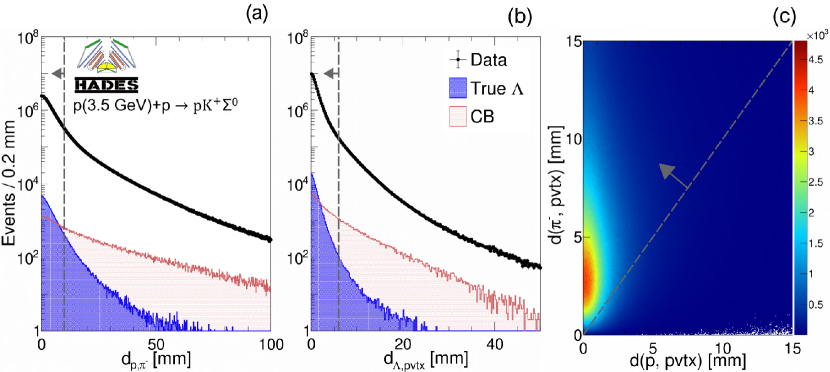
Figure 1: (a) The DCA distribution between the p and ^- tracks. (b) The DCA distribution between the track and the primary vertex. In both panels, data are shown by the black points, the blue histogram represents the true and the red histogram represents the CB, where both the true and the CB were estimated from the simulation. (c) Distribution of the DCA between the ^- track and the primary vertex as a function of the DCA between the p track and the primary vertex. The arrows indicate the accepted regions.

Since the daughter decays weakly ($c\tau$ = 7.89 cm), it can be identified by its displaced vertex. First, all possible combinations of the two p and ^- candidates were made, leaving the decision about which is the decay proton ( $\rightarrow$ p ^-) for later. For each combination the decay vertex (the displaced vertex) is defined as the PCA between the two tracks. The DCA between the p and ^- tracks (marked as $\mathrm{d_{p\pi^{-}}}$) is expected to be small if the tracks stem from the same vertex. Therefore, an upper limit of $\mathrm{d_{p\pi^{-}}}$ < 10 mm is imposed in order to reduce Combinatorial Background (CB), which originates from combining the wrong p and ^- pairs. Considering momentum and energy conservation, the p should be emitted in nearly the same direction as the in the laboratory reference frame, while the ^- will have a different direction. Thus, the DCA between the p track and the primary vertex ($\mathrm{d_{p,pvtx}}$) is required to be smaller than the DCA between the ^- track and the primary vertex ($\mathrm{d_{\pi^{-},pvtx}}$). Finally, the DCA between the calculated track and the primary vertex ($\mathrm{d_{\Lambda,pvtx}}$) is required to be < 6 mm. The distributions of the topological variables are shown in Figure 1, where the selection criteria are indicated by the vertical dashed lines. The proton used in the reconstruction is tagged as the decay proton (marked in the following as $\mathrm{p_{decay}}$), while the other proton in the event is tagged as the scattered (primary) proton.

To further purify the selected sample, the event kinematics were constrained to the ⁰ production range. The squared $\mathrm{p\Lambda}$ missing mass ($\mathrm{MM^{2}(pp_{decay}\pi^{-})}$) is required to be > 0.2 $\mathrm{GeV/c^{2}}$ in order to reject the multi-pion production channel as shown in Figure 2. In this figure, the experimental data are shown by the black points and the simulations (discussed in Section 3.4) by different colored histograms. Two peaks are visible, the first peak at 0.02 $\mathrm{GeV/c^{2}}$ corresponds to the multi-pion channel via the reaction $\mathrm{pp\rightarrow pp\pi^{+}\pi^{-}}$ (violet histogram), where a $\mathrm{p\pi^{-}}$ pair is incorrectly identified as a candidate and the ⁺ is incorrectly identified as a K⁺. The other broader peak is the sum of $\mathrm{pp\to pK^{+}\Lambda}$, $\mathrm{pp\rightarrow pK^{+}\Sigma^{0}}$ and $\mathrm{pp\to pK^{+}\Lambda\pi^{0}}$ reactions shown by the red, blue and green histograms, respectively. The relative normalizations of the simulated channels have been chosen to best fit the experimental data as explained in Section 3.4.

Figure 2: The squared p$\mathrm{p_{decay}}$ ^- missing mass distribution after applying the topological selections. Black points are the Spectrometer data-set data. The violet histogram is the $\mathrm{pp\rightarrow pp\pi^{+}\pi^{-}}$ simulation. The $\mathrm{pp\to pK^{+}\Lambda}$, $\mathrm{pp\rightarrow pK^{+}\Sigma^{0}}$ and $\mathrm{pp\to pK^{+}\Lambda\pi^{0}}$ simulations are shown by the red, blue and green histograms, respectively. The vertical line and the arrow indicate the accepted region for the further analysis.

The $\mathrm{p_{decay}}$ ^- invariant mass distribution is shown in Figure 3. A peak around the nominal mass is visible on top of background. The signal has been parameterized by a Voigt distribution and the background is modeled by a fourth-order polynomial. Events are further processed if they are in the range of $\mathrm{\mu\pm 3\sigma}$, where the calculated signal to background ratio in this range is $\mathrm{S/B=2.57}$ and the number of candidates is N_Λ = 6766.

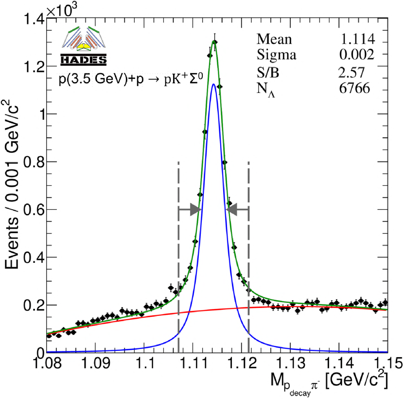
Figure 3: The $\mathrm{p_{decay}}$ ^- invariant mass distribution. The vertical dashed lines indicate the selected mass range. The blue, red and green curves are for the signal, background and the total fit.

The WALL data-set

In the WALL data-set the hit in the FW is assumed to be due to the decay proton. Since the FW is installed in a magnetic field-free region, the $\mathrm{p_{decay}}$ is reconstructed as a straight line trajectory from the primary vertex position to the hit in the FW. The track momentum is calculated from the $tof$ and the distance from the primary vertex and the FW detector hit, assuming the proton mass. In this case, the topological cuts are not as effective to suppress the background as in the Spectrometer data-set. Therefore, events fulfilling the following kinematical constraints were selected:

1. $\mathrm{MM^{2}(pp_{decay}\pi^{-})}$ > 0.2 $\mathrm{GeV/c^{2}}$ (Figure 4 a) and
   

2. The squared missing mass of all charged particles is required to be in the following range:
   $\mathrm{-0.02<MM^{2}(pK^{+}p_{decay}\pi^{-})[GeV^{2}/c^{4}]<0.01}$ because
   only a photon is missing to completely measure the exclusive final state (Figure 4 b).

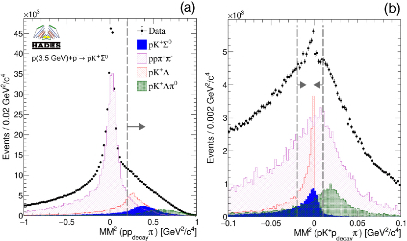
Figure 4: (a) The squared p$\mathrm{p_{decay}}$ ^- missing mass distribution of WALL data-set. (b) The squared p$\mathrm{p_{decay}}$ ^- K⁺ missing mass distributions. The $\mathrm{pp\rightarrow pp\pi^{+}\pi^{-}}$, $\mathrm{pp\to pK^{+}\Lambda}$, $\mathrm{pp\rightarrow pK^{+}\Sigma^{0}}$ and $\mathrm{pp\to pK^{+}\Lambda\pi^{0}}$ simulations are shown by the violet, red, blue and green histograms, respectively. The arrows indicate the accepted regions.

The $\mathrm{p_{decay}\pi^{-}}$ invariant mass distribution for the WALL data-set is shown Figure 5 after applying the selections mentioned above. Once again, the peak has been fitted by a Voigt distribution and the background by a fourth-order polynomial. However, the mass resolution of the peak of the Spectrometer data-set(Figure 3) is better than the signal of the WALL data-set, since in the latter case the proton was detected in the FW, which has a worse momentum resolution. Events are further processed if they are in the range of $\mathrm{\mu\pm 3\sigma}$, where the calculated signal to background ratio in this range is $\mathrm{S/B=1.56}$ and the number of candidates is N_Λ = 2340.

Figure 5: The $\mathrm{p_{wall}\pi^{-}}$ invariant mass distribution. The vertical dashed lines indicate the selected mass range. The blue, red and green curves are for the signal, background and the total fit.

3.4 ⁰ hyperon reconstruction

To further suppress the remaining background and to obtain a better mass resolution, a kinematic fit based on the Lagrange multiplier method is employed osti_837857 (27). The fit $\mathrm{\chi^{2}}$, expressed as

$$\chi^{2}(\eta,\lambda)=(y-\eta)^{T}V(y)(y-\eta)+2\lambda^{T}f(\eta)\>,$$

is minimized by differentiating $\chi^{2}$ with respect to all measured variables. Here $y$ is a vector containing the initial guesses for the measured quantities, which are the track parameters provided by the tracking algorithm, $\eta$ is an improved set of the track parameters and $V$ is the covariance matrix comprising the estimated errors on the measured quantities. The constraint equations are expressed as a function of $\eta$ in $f(\eta)$, where $\lambda_{i}$ are a set of Lagrange multipliers.

The spherical coordinates used in this analysis for the track parameterization are defined as follows

$$y=\begin{bmatrix}1/p\\ \theta\\ \phi\end{bmatrix}\>,$$

where $1/p$ is the inverse of the absolute momentum, $\theta$ and $\phi$ are the polar and azimthual angles of the track.

Two constraints were applied to both data-sets. The first is the proton and pion from the decay are constrained to the mass ($\mathrm{M_{\Lambda}}=$ 1.1157 $\mathrm{GeV/c^{2}}$). The second constraint is that the missing mass of all the charged final state particles is constrained to the photon mass ($\mathrm{M_{\gamma}}=$ 0 $\mathrm{GeV/c^{2}}$).

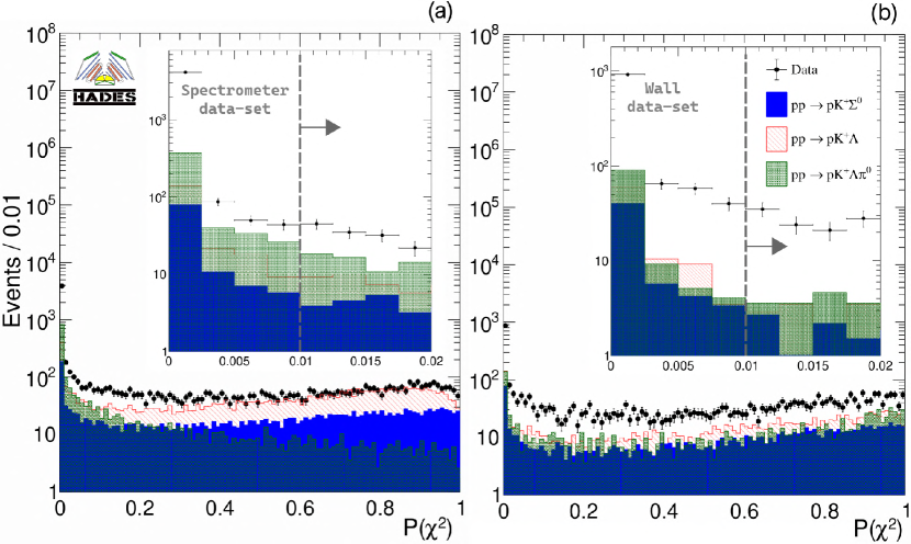
Figure 6: (a) The p-value distributions for the HADES data-set and for (b) the WALL data-set. The insets display the region of small p-values, where the dashed line and the arrow indicates the accepted region. The $\mathrm{pp\to pK^{+}\Lambda}$, $\mathrm{pp\rightarrow pK^{+}\Sigma^{0}}$ and $\mathrm{pp\to pK^{+}\Lambda\pi^{0}}$ simulations are shown by the red, blue and green histograms, respectively.

The probability that a $\mathrm{\chi^{2}}$ of the theoretical distribution is greater than or equal to the $\mathrm{\chi^{2}}$ value found from the fit is known as the p-value ($\mathrm{P(\chi^{2})}$). The p-value distributions of the Spectrometer and the WALL data-sets are shown in Figure 6. Because both and ⁰ have $\mathrm{MM(pK^{+}\Lambda)}$ = 0, they have similar distributions, which makes these two reactions difficult to distinguish. On the other hand, the reaction $\mathrm{pp\to pK^{+}\Lambda\pi^{0}}$ should ideally have zero p-value. However, due to the limited detector resolution it has p-values greater than zero, which is more pronounced in the WALL data-set. The signal events show an almost flat distribution between 0 and 1, while events that do not satisfy the constraint equations have a prominent yield of p-values close to 0. Therefore, events with p-values > 0.01 are selected, where the cut was optimized based on a significance analysis.

Simulation scaling to the experimental data

By inspecting the $\mathrm{pK^{+}}$ missing mass distribution of the combined data-set shown in Figure 7, two peaks corresponding to the and the ⁰, as well as other minor contributions in the high mass region, are plainly evident. In order to quantify the different contributions an incoherent cocktail has been simulated using the Pluto event generator Frohlich:2007bi (28). All the simulated reactions have been processed using the same full scale analysis employed for the experimental data, thus taking into account the efficiency of the trigger condition, the tracking algorithm and the analysis procedure. The particle decays, the acceptance and the particle interactions with the materials of HADES and the FW have been considered by using GEANT3 Brun:1994aa (29).

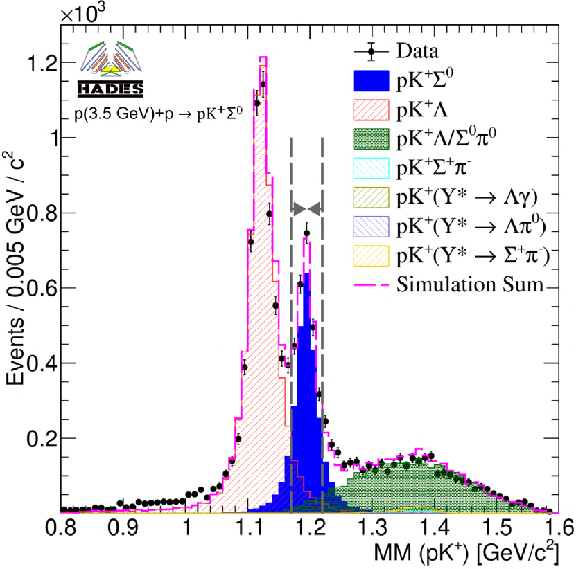
Figure 7: The $\mathrm{pK^{+}}$ missing mass distribution. The colored histograms represent the simulated channels, where Y^∗ refers to an excited hyperon ((1385), (1405) or (1520)). The two peaks are due to the exclusive reactions $\mathrm{pp\to pK^{+}\Lambda}$ and $\mathrm{pp\rightarrow pK^{+}\Sigma^{0}}$ as shown by the red and the blue histograms, respectively. The vertical dashed lines mark the mass window used to select candidate events of the $\mathrm{pp\rightarrow pK^{+}\Sigma^{0}}$ final state.

To determine the contributions of the different channels, a fit of the simulations to the measured missing mass spectrum ($\mathrm{MM(pK^{+})}$) has been carried out by minimizing the quantity

$$\chi^{2}=\sum_{i}^{n_{bins}}\frac{(n_{data}-\sum_{ch}(f^{ch}\times n^{ch}_{simulation}))^{2}}{\sigma_{data}^{2}+\sigma_{simulation}^{2}}\>,$$

where the summation runs over the number of bins of the missing mass spectrum, $\mathrm{n_{data}}$ is the number of data events in each bin, $\mathrm{n^{ch}_{simulation}}$ is the number of simulated events in each bin for each channel and $\mathrm{f^{ch}}$ is a scaling factor for each channel. The uncertainty for the data and the simulations in each bin is $\mathrm{\sigma_{data}}$ and $\mathrm{\sigma_{simulation}}$, respectively.

As can be seen from Figure 7, the experimental data is primarily described by contributions of $\mathrm{pp\to pK^{+}\Lambda}$,
$\mathrm{pp\rightarrow pK^{+}\Sigma^{0}}$ and $\mathrm{pp\to pK^{+}\Lambda\pi^{0}}$ indicated by the red, blue and the green histogram, respectively. The other simulated channels have minor contributions. In total 2613 ⁰ candidates were collected within the $\mathrm{pK^{+}}$ missing mass range of 1.170-1.220 $\mathrm{GeV/c^{2}}$, 58% of them are within the main HADES acceptance and 42% within the FW acceptance. The signal purity in the mass window calculated from the simulation is found to be 81%, where the main background contributions are the reactions $\mathrm{pp\to pK^{+}\Lambda}$ (14%) and $\mathrm{pp\to pK^{+}\Lambda\pi^{0}}$ (5%).

3.5 Efficiency and acceptance correction

The reconstructed experimental distributions are corrected for the limited detector acceptance and efficiency by using a simulated phase space distribution that were assigned a weight determined by the best partial wave solution (discussed in Section 6), then the events were filtered through the full scale simulation and analysis. The efficiency correction is done in one dimension whereas the other three degrees of freedom on which the efficiency depends are integrated.

The 1D correction matrix (M) is calculated given the initial 4$\pi$ distribution (T) for each observable and after filtering through the full scale simulation and analysis (R). To put it another way, a distinct correction matrix M = R/T is constructed for each angular distribution shown in Figure 8. The inverse of the correction matrix is then calculated using the Singular Value Decomposition (SVD) technique Hocker:1995kb (30) implemented in RooUnfold framework Adye:2011gm (31).

3.6 Absolute normalization and systematic uncertainties

The production cross section of ⁰ can be calculated by normalizing the corrected ⁰ yield to the p+p elastic scattering yield measured in the same experimental run HADES:2011ab (32). This normalization results in a systematic uncertainty of 7%. In addition, there might be other sources of systematic uncertainty. The systematic error associated to the exclusive event selection has been estimated by varying the selection ranges and recalculating the cross section.

To test the influence of different selection cuts on the calculated cross section (see section 5), the whole analysis chain has been repeated many times under different cut combinations. Each cut is varied in two steps in either direction. the cross section for each combination is then calculated by integrating the yield of the $\mathrm{cos\theta^{*}_{\Sigma^{0}}}$ angular distribution. Following this procedure the obtained systematic error, defined as the 1$\mathrm{\sigma}$ interval of the cross sections distribution, is found to be $\approx$ 2%.

Another source of the systematic errors is the PID, which is evaluated by activating the dropout layers of the neural network during the inference time as this is equivalent to doing a Bayesian approximation pmlr-v48-gal16 (33). The estimated size of the PID systematic is $\approx$ 5%.

4 Angular Distributions

This section presents the differential cross section of the reaction $\mathrm{pp\rightarrow pK^{+}\Sigma^{0}}$, namely the angular distributions of final state particles in the center-of-mass (CMS) frame, as well as in both the Gottfried-Jackson and helicity frames of all two-body subsystems. All distributions are acceptance and efficiency corrected and then fit with Legendre polynomials $d\sigma/dcos\theta$ = $\sum_{l}A_{l}\cdot P_{l}$, with $l$ = $0,1,2$. The coefficients $A_{1}$ and $A_{2}$ are used to judge the asymmetries and anisotropies of the observed distributions. The best description of the distribution (indicated by the blue histogram in Figure 8) was found when the simulations have been weighted simultaneously with the angular distribution of the ⁰ hyperon in the CMS frame and the proton Gottfried-Jackson angular distribution measured in the $\mathrm{p\Sigma^{0}}$ rest frame obtained from the data.

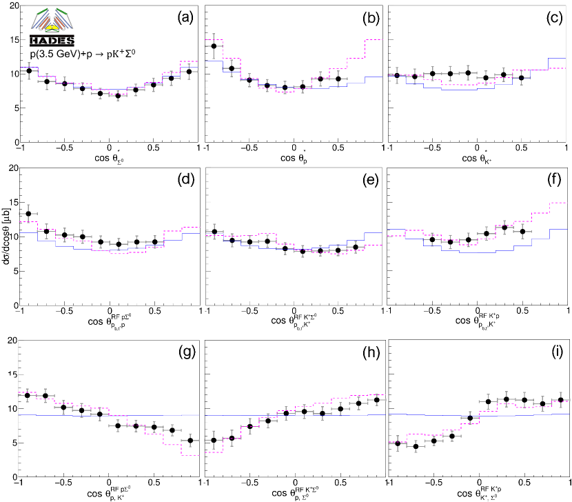
Figure 8: The corrected angular distributions in the CMS (top row), Gottfried-Jackson (middle row) and helicity frames (bottom row). The experimental data are shown by the black points, where the error bars are the square root of the quadratic sum of the statistical and systematic uncertainties. The blue histogram represent the weighted $\mathrm{pp\rightarrow pK^{+}\Sigma^{0}}$ phase space simulation described in the text and the dotted pink histogram indicates the best partial wave analysis solution (discussed in Section 6).

Table 1: Coefficients of Legendre polynomials determined by fitting the angular distributions presented in Figure 8.

Angle	A0 [$\mathrm{\mu b}$]	A1 [$\mathrm{\mu b}$]	A2 [$\mathrm{\mu b}$]
$\mathrm{cos\theta^{*}_{\Sigma^{0}}}$	8.55 $\pm$ 0.31	0.00	2.75 $\pm$ 0.73
$\mathrm{cos\theta^{*}_{p}}$	10.01 $\pm$ 0.50	0.00	4.33 $\pm$ 1.27
$\mathrm{cos\theta^{*}_{K^{+}}}$	9.83 $\pm$ 0.43	0.00	-0.13 $\pm$ 1.02
$\mathrm{cos\theta^{FRp\Sigma^{0}}_{p_{b,t},p}}$	10.40 $\pm$ 0.80	-0.64 $\pm$ 1.73	2.79 $\pm$ 1.85
$\mathrm{cos\theta^{FRK^{+}\Sigma^{0}}_{p_{b,t},K^{+}}}$	8.55 $\pm$ 0.71	-1.61 $\pm$ 1.54	0.66 $\pm$ 1.63
$\mathrm{cos\theta^{FRK^{+}p}_{p_{b,t},K^{+}}}$	10.30 $\pm$ 1.00	1.91 $\pm$ 1.18	0.50 $\pm$ 2.69
$\mathrm{cos\theta^{FRK^{+}\Sigma^{0}}_{p,\Sigma^{0}}}$	8.70 $\pm$ 0.30	3.17 $\pm$ 0.59	-0.73 $\pm$ 0.75
$\mathrm{cos\theta^{FRp\Sigma^{0}}_{p,K^{+}}}$	8.75 $\pm$ 0.29	-3.52 $\pm$ 0.50	0.37 $\pm$ 0.67
$\mathrm{cos\theta^{FRK^{+}p}_{K^{+},\Sigma^{0}}}$	8.81 $\pm$ 0.31	4.84 $\pm$ 0.56	-0.98 $\pm$ 0.75

Center of mass frame

The angular distributions of the three final state particles in the CMS are shown in the top row of Figure 8. The Legendre polynomial coefficients obtained from the fits of the angular distributions are listed in Table 1. Since the initial p+p is a symmetric system, the $A_{1}$ Legendre parameters of all CMS distributions were set to zero. The angular distribution of the ⁰ hyperon (Figure 8 (a)) and proton (Figure 8 (b)) shows an anisotropy, where it is more pronounced for the proton as quantified by the $\mathrm{A_{2}}$ parameter listed in Table 1. From the observed anisotropies and the fit parameters one deduces that a non-zero orbital angular momentum ($L$) is observed in both the $\mathrm{p-K^{+}\Sigma^{0}}$ and $\mathrm{\Sigma^{0}-pK^{+}}$ sub-systems. This is in contrast to the kaons, where the angular distribution is compatible with isotropy. For pure pion exchange, the final state proton is the leading particle, since the exchange pion has a small mass, implying a small 4-momentum transfer so that the proton is preferably emitted in the direction of the initial protons, which could explain the anisotropy in the proton angular distribution. In this picture, the ⁰ CMS angular distribution reflects the proton one, while the kaon has a broader distribution.

The angular distributions in the overall CMS are not suited to directly draw conclusions on resonant production, which proceeds as a two step process pp → pR, R → K^{+ 0}, where R stands for every kind of nucleon resonance, that can be either an isospin 1/2 $\mathrm{N^{*}}$ state or an isospin 3/2 $\mathrm{\Delta^{*}}$ state. Therefore in the following the Gottfreid-Jackson and helicity frames are presented as a more natural choice for the Lorentzian reference frames in order to study the reaction properties due to resonant production.

Gottfried-Jackson frames

The Gottfried-Jackson (G-J) frame first introduced in Gottfried:1964nx (34) is the rest frame of two out of the three produced particles. In the G-J frame, the G-J angle is defined as the angle between one of the rest frame particles (e.g. the ⁰) and the initial proton $\mathrm{\theta^{RF\,K^{+}\Sigma^{0}}_{p_{b,t},\Sigma^{0}}}$, where the label RF stands for reference frame, the superscript indicates which rest frame is used and the subscript stands for the two particles, between which the angle is measured. It should be noted that the two initial protons are indistinguishable. Therefore, the angular distribution is calculated by using the angle to both protons ($\mathrm{p_{b,t}}$).

In the case of kaon (pion) exchange, the $\mathrm{K^{+}p}$ ($\mathrm{K^{+}\Sigma^{0}}$) rest frame is equivalent to the rest frame of the exchanged meson and the initial proton. In this way, the initial 2 → 3 reaction is reduced to a pure 2 → 2 reaction. If there is a resonant production, the internal angular momentum of the resonance is then reflected in this observable. It has to be noted that the distributions in the G-J frames do not have to be symmetric. The reason is the asymmetric reaction system, where either a kaon or a pion collides with a proton. The angular distributions in the G-J frames are shown in the middle row of Figure 8.

An anisotropy is observed in the $\mathrm{p\Sigma^{0}}$ G-J frame (Figure 8 (d)), which could be due to a relative angular momentum in the $\mathrm{p\Sigma^{0}}$ system. This effect is related to the above mentioned anisotropies of the p and ⁰ CMS angular distributions since they are kinematically related. The angular distribution in the in $\mathrm{K^{+}\Sigma^{0}}$ G-J frame (Figure 8 (e)) tends to be asymmetric, which could be caused by the excitation of nucleon resonances decaying into the $\mathrm{K^{+}\Sigma^{0}}$ channel AbdelBary:2010pc (2). Many of $\mathrm{N^{*}}$ or $\mathrm{\Delta^{*}}$ resonances could contribute to the reaction. All these resonances have large widths and may also contribute through their broad tails to the reaction. The angular distribution of a true two-body resonance reaction is asymmetric only if resonances with both parities are simultaneously excited through interfering amplitudes. Hence, this distribution in the $\mathrm{K^{+}\Sigma^{0}}$ G-J frame indicates that more than one nucleon resonance with opposite parity participates in the production process AbdelBary:2010pc (2). As explained earlier, the $\mathrm{K^{+}p}$ rest frame is equivalent to the rest frame of the exchanged kaon. Therefore, the deviation from isotropy in the $\mathrm{cos\theta^{FRK^{+}p}_{p_{b,t},K^{+}}}$ angular distribution could be explained by kaon exchange component Esmail:2022fdy (25). For a pure pion exchange, the Treiman-Yang (T-Y) angle measured in the $\mathrm{K^{+}\Sigma^{0}}$ rest frame is expected to be an isotropic distribution Ferrari:1968bbl (35). Therefore, if a kaon exchange contributes to the production mechanism it should reflect itself in this distribution. The ⁰ hyperon T-Y angle measured in the $\mathrm{K^{+}\Sigma^{0}}$ rest frame, shown in Figure 9, shows a clear deviation from isotropy, which could be an indication of a significant kaon exchange contribution to the reaction mechanism.

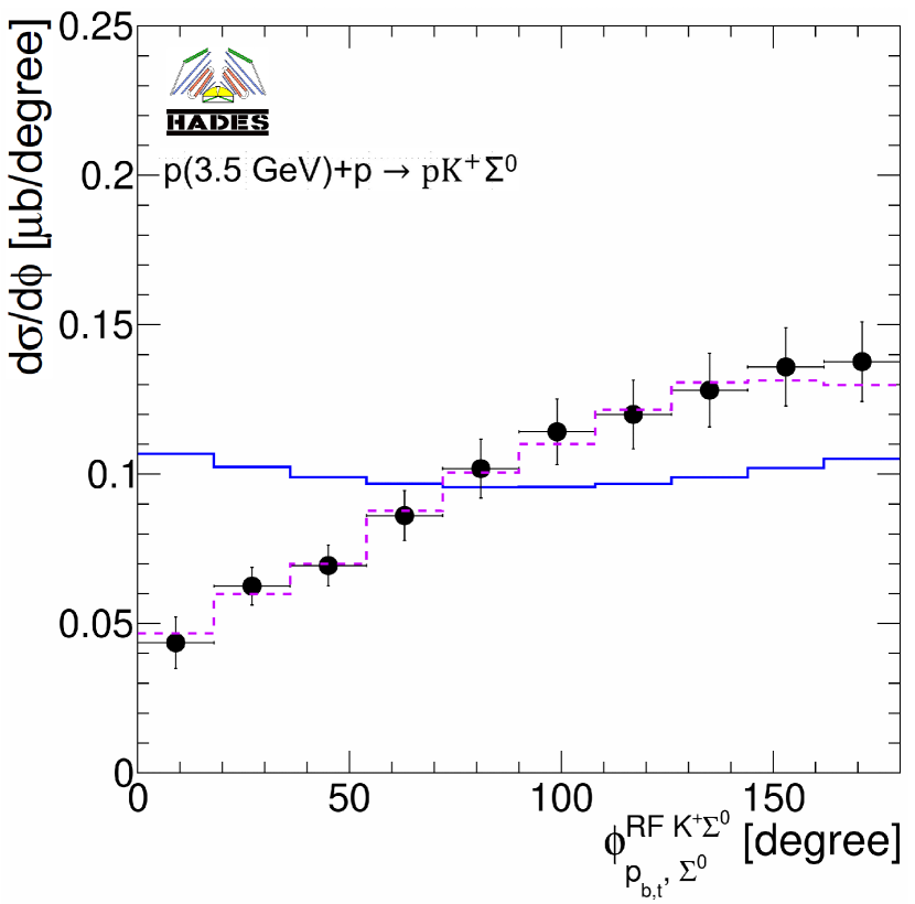
Figure 9: The ⁰ Treiman-Yang angular distribution measured in the $\mathrm{K^{+}\Sigma^{0}}$ reference frame. The blue histogram represents the weighted $\mathrm{pp\rightarrow pK^{+}\Sigma^{0}}$ phase space simulation and the dotted histogram indicates the best partial wave analysis solution (discussed in Section 6).

Helicity frames

The helicity angle is defined in a similar way as the G-J angle, but instead of calculating the angle of the respective particle to the initial proton, the helicity angle is calculated between one of the rest frame particles and the third produced particle. The helicity angular distribution thus interrelates the kinematics of the three final state particles and it is thus a linear transformation projection of the Dalitz plot. A uniformly populated Dalitz plot results in isotropic helicity angle distributions. On the other hand, if dynamical effects distort the Dalitz plot, then the helicity angular distribution will be anisotropic. The helicity angular distributions are shown in the bottom row of Figure 8. All the distributions are significantly non-isotropic, which indicates that the reaction is dominated by intermediate resonances. Therefore, an inclusion of intermediate resonances is necessary in order to quantitatively describe experimental angular distributions.

Comparison to lower energy

A comparison of the normalized Legendre coefficients between this measurement and data collected at a lower value of excess energy $\epsilon$ = 162 MeV AbdelBary:2010pc (2) is listed Table 2. The two sets of coefficients show striking differences for few coefficients indicating that the ⁰ production mechanism changes between these values of excess energy. The CMS distributions are more forward-backward peaked for the proton and the ⁰ hyperon and less peaked for the kaon, pointing to a larger relative contribution of pion with respect to kaon exchange at larger energies. In addition, the helicity angle distributions have a significant asymmetry at the highest energy, in contrast with the lower energy results.

Table 2: Comparison of the normalized Legendre coefficients between the present measurement and the data collected by COSY-TOF experiment at $\mathrm{\epsilon}=162$ MeV AbdelBary:2010pc (2).

	$\epsilon$ = 162 MeV		$\epsilon$ = 556 MeV
	$A_{1}/A_{0}$	$A_{2}/A_{0}$	$A_{1}/A_{0}$	$A_{2}/A_{0}$
$\mathrm{cos\theta^{CMS}_{\Sigma^{0}}}$	0.0 $\pm$ 0.0	0.03 $\pm$ 0.24	0.0 $\pm$ 0.0	0.32 $\pm$ 0.09
$\mathrm{cos\theta^{CMS}_{p}}$	0.0 $\pm$ 0.0	0.25 $\pm$ 0.29	0.0 $\pm$ 0.0	0.43 $\pm$ 0.13
$\mathrm{cos\theta^{CMS}_{K^{+}}}$	0.0 $\pm$ 0.0	0.48 $\pm$ 0.22	0.0 $\pm$ 0.0	-0.01 $\pm$ 0.1
$\mathrm{cos\theta^{FRp\Sigma^{0}}_{p_{b,t},p}}$	0.0 $\pm$ 0.0	0.11 $\pm$ 0.15	-0.06 $\pm$ 0.17	0.27 $\pm$ 0.18
$\mathrm{cos\theta^{FRK^{+}\Sigma^{0}}_{p_{b,t},K^{+}}}$	-0.04 $\pm$ 0.04	0.14 $\pm$ 0.18	-0.19 $\pm$ 0.18	0.08 $\pm$ 0.19
$\mathrm{cos\theta^{FRK^{+}p}_{p_{b,t},K^{+}}}$	-0.07 $\pm$ 0.07	0.57 $\pm$ 0.18	0.19 $\pm$ 0.12	0.05 $\pm$ 0.26
$\mathrm{cos\theta^{FRK^{+}\Sigma^{0}}_{p,\Sigma^{0}}}$	0.27 $\pm$ 0.27	-0.15 $\pm$ 0.15	0.36 $\pm$ 0.07	-0.08 $\pm$ 0.09
$\mathrm{cos\theta^{FRp\Sigma^{0}}_{p,K^{+}}}$	-0.22 $\pm$ 0.22	0.0 $\pm$ 0.15	-0.4 $\pm$ 0.06	0.04 $\pm$ 0.08
$\mathrm{cos\theta^{FRK^{+}p}_{K^{+},\Sigma^{0}}}$	-0.11 $\pm$ 0.11	0.11 $\pm$ 0.18	0.55 $\pm$ 0.07	-0.11 $\pm$ 0.09

5 Total Cross Section

The total production cross section as function of the excess energy $\epsilon$ is used as a tool to compare the experimental data to the different theoretical approaches. The result on the $\mathrm{pp\rightarrow pK^{+}\Sigma^{0}}$ production cross section, obtained by integrating the $cos\mathrm{\theta^{*}_{\Sigma^{0}}}$ angular distribution, is

$$\sigma(pK^{+}\Sigma^{0})[\mu b]=17.7\pm 1.7(stat)\pm 1.6(syst)\>.$$

The cross section value is included in Figure 10, which shows a compilation of the $\mathrm{pp\rightarrow pK^{+}\Sigma^{0}}$ cross sections as a function of the excess energy. The present data point corresponds to $\epsilon$ = 556 MeV, which is depicted by the green square and existed in a region where no other measurements have been performed. This behaviour can not be described by phase space within experimental uncertainty as clearly seen by the solid curve $\sigma_{pK^{+}\Sigma^{0}}=K\epsilon^{2}$, where the quadratic excess-energy dependence is attributed to a pure (i.e. trivial) three-body phase space and $K$ is the fit free parameter.

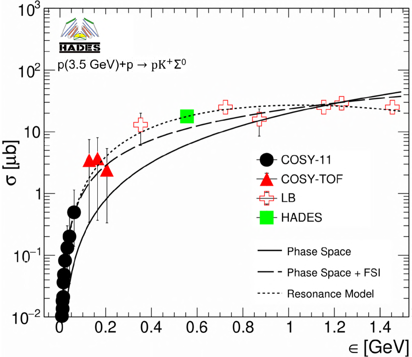
Figure 10: Compilation of cross sections of the reaction $\mathrm{pp\rightarrow pK^{+}\Sigma^{0}}$ from different experiments: COSY-11 GRZONKA199741 (36, 37, 38, 39, 40, 41), COSY-TOF AbdelBary:2010pc (2) and data points from Landolt-Börnstein (LB) Schopper:214138 (42). The production cross section of ⁰ determined here is shown by the green square. The solid curve represents a pure phase space fit, the dotted curve is a parametrization based on the resonance model and the dashed curve is phase space and FSI as described in the text.

An alternative parametrization proposed by Fäldt and Wilkin in Faldt:1996rh (43) that takes the proton-hyperon FSI interaction into account

$$\sigma=C\cdot\frac{\epsilon^{2}}{(1+\sqrt{1+\epsilon/\alpha})^{2}}\>,$$

where the parameters $C=7.82\times 10^{2}\mu b$ $GeV^{-2}$ and $\alpha=4.57\times 10^{-2}GeV$ are related to the FSI strength. Interestingly, the deviations to the pure phase space behavior start showing up at $\epsilon$ $>$ 200 MeV. The displayed data in that region could also be approximated by $\sigma$ $\approx$ 10 $\mu b$.

A more appropriate paramerization proposed by Tsushima in Tsushima:1998jz (44) shown by the dotted line is based on a resonance model, where the hyperon is produced via an intermediate nucleon resonance $\mathrm{N^{*}}$ or $\mathrm{\Delta^{*}}$. This paramerization describes all data points near threshold up to 1.4 GeV fairly well.

Using the $\mathrm{pp\rightarrow pK^{+}\Lambda}$ cross section measured by the HADES collaboration Agakishiev:2014dha (22), the cross section ratio $\sigma(pK^{+}\Lambda)/\sigma(pK^{+}\Sigma^{0})$ is determined to be 1.90 $\pm$ 0.41. Based on the coupled channel calculation, where the interference of the pion and kaon exchange is taken in account, the cross section ratio can be reproduced by selecting the relative sign for these two mechanism Kowina:2004kr (17). Figure 11 shows the cross section ratio as a function of the excess energy together with a compilation of other measurements Schopper:214138 (42). The solid curve is the ratio of the paramerization of both channels, where the paramerization proposed by Fäldt and Wilkin Faldt:1996rh (43) based on phase space and FSI is used for $\mathrm{pp\to pK^{+}\Lambda}$ and the Tsushima paramerization Tsushima:1998jz (44) based on a resonance model is used for the $\mathrm{pp\rightarrow pK^{+}\Sigma^{0}}$ channel.

The observed cross section ratio in the present p+p data is similar to the corresponding value measured in p+Nb data Adamczewski-Musch:2017gjr (7), despite the large difference in the individual cross sections, thus corroborating the importance of FSI for these reactions.

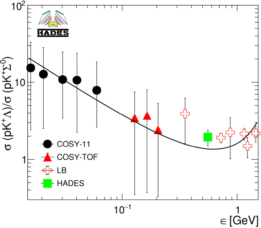
Figure 11: Experimental cross section ratio of the present data point together with a compilation of the world data: COSY-11 GRZONKA199741 (36, 37, 38, 39, 40, 41), COSY-TOF AbdelBary:2010pc (2) and data points from Landolt-Börnstein (LB) Schopper:214138 (42). The present data square is shown by the green square. The solid curve is the ratio of the paramerization of both channels Faldt:1996rh (43, 44).

6 Partial Wave Analysis

From the results presented above, it was concluded that the experimental data on angular distributions can not be described by pure phase space production, but there must be a resonant component as anticipated in AbdelBary:2010pc (2). Therefore, a Partial Wave Analysis (PWA) using the Bonn-Gatchina Partial Wave Analysis (Bo-Ga PWA) framework Sarantsev:2005tg (45) has been applied with the goal to quantify the relative contributions of different partial waves.

The Bo-Ga PWA framework takes a list of possible transition waves as an input that may contribute to the final state. The non-resonant production proceeds as follows: the proton ($\mathrm{J^{P}}$= $\frac{1}{2}^{+}$) and the hyperon (in this case ⁰ with $\mathrm{J^{P}}$= $\frac{1}{2}^{+}$) are combined into a two particle sub-system and then the kaon ($\mathrm{J^{P}}$= $0^{-}$) is combined with this sub-system to produce the three-body final state. In case of the resonant production, the proton is combined with one of the resonances listed in Table 3 $\mathrm{N^{*}}$-p, or $\mathrm{\Delta^{*}}$-p to produce the final state $\mathrm{pp\rightarrow pK^{+}\Sigma^{0}}$. Resonance masses and widths were fixed to the PDG values Tanabashi:2018oca (46) in order to reduce the number of the free fit parameters.

Table 3: A list of $\mathrm{N^{*}}$ and $\mathrm{\Delta^{*}}$ resonances that might contribute to the $\mathrm{pp\rightarrow pK^{+}\Sigma^{0}}$ reaction. The mass, width and spin-parity quantum numbers were taken from Tanabashi:2018oca (46).

Resonance	Mass [$\mathrm{GeV/c^{2}}$ ]	Width [$\mathrm{GeV/c^{2}}$ ]	$\mathrm{J^{P}}$
$\mathrm{N^{*}(1710)}$	1.710	0.140	$\frac{1}{2}^{+}$
$\mathrm{N^{*}(1875)}$	1.875	0.200	$\frac{3}{2}^{-}$
$\mathrm{N^{*}(1880)}$	1.880	0.300	$\frac{1}{2}^{+}$
$\mathrm{N^{*}(1895)}$	1.895	0.120	$\frac{1}{2}^{-}$
$\mathrm{N^{*}(1900)}$	1.920	0.200	$\frac{3}{2}^{+}$
$\mathrm{\Delta^{*}(1900)}$	1.860	0.250	$\frac{1}{2}^{-}$
$\mathrm{\Delta^{*}(1910)}$	1.900	0.300	$\frac{1}{2}^{+}$
$\mathrm{\Delta^{*}(1920)}$	1.920	0.300	$\frac{3}{2}^{+}$

The strength ($\mathrm{\alpha_{1}}$) and the phase ($\mathrm{\alpha_{2}}$) of each transition wave are determined by fitting the partial wave amplitudes to the experimental data on an event-by-event basis in an unbinned fit. The fit is based on a log-likelihood minimization and the fitting procedure is repeated for many iterations until there is no further improvement of the log-likelihood value. By comparing the log-likelihood value of many fits the best fit can be determined through the largest negative value. As an output, the BG-PWA returns the fitted values of the parameters $\mathrm{\alpha_{1}}$ and $\mathrm{\alpha_{2}}$ and a list of simulated events that have been used as an input but with each event being assigned a weight factor, which gives the contribution of this event to the total yield.

Since the signal region contains background events (mainly $\mathrm{pp\to pK^{+}\Lambda}$ and $\mathrm{pp\to pK^{+}\Lambda\pi^{0}}$), and because the Bo-Ga PWA method works on an event-by-event basis, it is important to identify whether a particular event belongs to the signal or the background. The $\mathrm{pp\to pK^{+}\Lambda}$ contribution is three times larger than $\mathrm{pp\to pK^{+}\Lambda\pi^{0}}$ inside the signal region. Therefore, the $\mathrm{pp\to pK^{+}\Lambda}$ channel is considered the main contributing background and its kinematics is modeled by performing a PWA on the $\mathrm{pp\to pK^{+}\Lambda}$-like events. The solutions published in Agakishiev:2014dha (22) have been tested and solution No. 8/1 was found to provide the best description of the experimental data by including the p+p initial waves ${}^{2S+1}L_{J}$ = ${}^{1}S_{0}$, ${}^{3}P_{0}$, ${}^{3}P_{1}$ and ${}^{1}D_{2}$.

The solution No. 8/1 is then applied to the 4$\pi$-phase space simulations and these events are filtered through the full simulation and analysis chain. After reconstructing the events that have been assigned a PWA weight, the missing mass $\mathrm{MM(pK^{+})}$ spectrum was investigated and the contribution in the signal region $\mathrm{1.170<MM(pK^{+})[GeV/c^{2}]<1.220}$ was determined to be 292 events. Those events are then added to the signal list with a negative weight.

After subtracting the contribution, the PWA technique is applied to the $\mathrm{pp\rightarrow pK^{+}\Sigma^{0}}$ events. A systematic variation of the input partial waves was performed and, in addition, the number of non-resonant and resonant final partial waves was varied and the quality of the PWA solution was determined by the negative log-likelihood value of the fit.

The best PWA solution shown by the dashed histograms in Figures 8 and 9 was obtained by including p+p initial waves ${}^{2S+1}L_{J}$ = ${}^{2}S_{0}$, ${}^{3}P_{0}$, ${}^{3}P_{1}$, ${}^{3}P_{2}$, ${}^{1}D_{2}$ and ${}^{3}F_{2}$. In addition, nucleon resonances $\mathrm{N^{*}(1710)}$, $\mathrm{N^{*}(1900)}$ and $\mathrm{\Delta^{*}(1900)}$ were found to contribute as well as non-resonant partial waves. However, due to the limited statistics and the large number of free fit parameters, an unambiguous determination of the contributions of each resonance is not possible since these contributions vary significantly for different solutions. Nevertheless, resonances with masses around 1.710 $\mathrm{GeV/c^{2}}$ ($\mathrm{N^{*}(1710)}$) and 1.900 $\mathrm{GeV/c^{2}}$ ($\mathrm{N^{*}(1900)}$ or $\mathrm{\Delta^{*}(1900)}$) are certainly preferred by the fit.

7 Conclusion and Outlook

The exclusive reconstruction of the reaction $\mathrm{pp\rightarrow pK^{+}\Sigma^{0}}$ at a beam kinetic energy of 3.5 GeV has been presented and the $\mathrm{pp\rightarrow pK^{+}\Sigma^{0}}$ total production cross section was determined with an accuracy better than 10 % in a region where no data existed. The dynamics of the reaction was investigated by studying the angular distributions in the CMS, G-J and helicity frame. The corrected CMS distributions of the hyperon and the proton show anisotropies, which it is more pronounced in the case of the proton. This is the expected behavior if the pion exchange mechanism dominates the particle production process in a simple one-boson exchange formalism. In addition, an investigation of the ⁰ T-Y angle measured in the $\mathrm{K^{+}\Sigma^{0}}$ reference frame, deviates from isotropy, which hints to a non-negligible contribution of the of kaon exchange mechanism.

The helicity angular distributions are not isotropic, which indicates that a pure phase space description without momentum-dependent matrix element(s) is by far not appropriate. The influence of different nucleon resonances has been tested by means of a PWA using the Bo-Ga PWA framework. The best solution was obtained by including the initial p+p configuration ${}^{1}S_{0}$, ${}^{3}P_{0}$, ${}^{3}P_{1}$, ${}^{3}P_{2}$, ${}^{1}D_{2}$ and ${}^{3}F_{2}$. Due to the limited statistics, it was not possible to obtain the exact strength of the individual nucleon resonances. However, nucleon resonances $\mathrm{N^{*}(1710)}$, $\mathrm{N^{*}(1900)}$ and $\mathrm{\Delta^{*}(1900)}$ are preferred by the fit.

Recently, the HADES setup has been upgraded by an electromagnetic calorimeter (ECAL) and a Forward Detector (FD) based on PANDA experiment straw tubes Adamczewski-Musch:2021rlv (47). The new data that was collected in February 2022 offers the opportunity to perform the same measurement with an upgraded setup at a higher proton beam energy of 4.5 GeV. This upgrade will allow the identification of the daughter photon in $\mathrm{\Sigma^{0}\rightarrow\Lambda\gamma}$ via the ECAL. In addition, it will improve the mass resolution of the hyperon in the FD acceptance and consequently improve the quality of the kinematic refit. Furthermore, the collected data will provide sufficient statistics to extract quantitative contributions of the different nucleon resonances and a measurement of their $\mathrm{K^{+}\Sigma^{0}}$ branching ratios, which will certainly improve the current measurement.

8 Acknowledgment

The HADES collaboration gratefully acknowledges the support by SIP JUC Cracow, Cracow (Poland), 2017/26/M/ST2/00600; WUT Warsaw (Poland) No: 2020/38/E/ST2/00019 (NCN), IDUB-POB-FWEiTE-3; TU Darmstadt, Darmstadt (Germany), VH-NG-823, DFG GRK 2128, DFG CRC-TR 211, BMBF:05P18RDFC1, HFHF, ELEMENTS 500/10.006, GSI F&E, EMMI at GSI Darmstadt; Goethe-University, Frankfurt (Germany), BMBF:05P12RFGHJ, GSI F&E, HIC for FAIR (LOEWE), EMMI at GSI Darmstadt; JLU Giessen, Giessen (Germany),BMBF:05P12RGGHM; IJCLab Orsay, Orsay (France), CNRS/IN2P3; NPI CAS, Rez, Rez (Czech Republic), MSMT LTT17003, MSMT LM2018112, MSMT OP VVV CZ.02.1.01/0.0/0.0/18_046/0016066; European Union’s Horizon 2020, no. 824093 (STRONG2020).
This project has received funding from the programme ”Netzwerke 2021”, an initiative of the Ministry of Culture and Science of the State of Northrhine Westphalia. The sole responsibility for the content of this publication lies with the authors.
The following colleagues from Russian institutes did contribute to the results presented in this publication but are not listed as authors following the decision of the HADES Collaboration Board on March 23, 2022: G. Agakishiev, A. Belyaev, O. Fateev, A. Ierusalimov, V. Ladygin, T. Vasiliev, M. Golubeva, F. Guber, A. Ivashkin, T. Karavicheva, A. Kurepin, A. Reshetin, A. Sadovsky and A.V.Sarantsev.

References

- (1) G.. Brown, C.. Ko, Z.. Wu and L.. Xia “Kaon production from hot and dense matter formed in heavy ion collisions” In Phys. Rev. C 43, 1991, pp. 1881–1892 DOI: 10.1103/PhysRevC.43.1881
- (2) M. Abdel-Bary “Production of and hyperons in proton-proton collisions” In Eur. Phys. J. A 46, 2010, pp. 27–44 DOI: 10.1140/epja/i2010-11023-0
- (3) J. Adamczewski-Musch “Inclusive production in proton-proton collisions at 3.5 GeV” In Phys. Rev. C 95, 2017, pp. 015207 DOI: 10.1103/PhysRevC.95.015207
- (4) G. Agakishiev “Lambda hyperon production and polarization in collisions of p(3.5 GeV)+Nb” In Eur. Phys. J. A 50, 2014, pp. 81 DOI: 10.1140/epja/i2014-14081-2
- (5) J. Balewski “-hyperon production via the reaction 2-MeV above threshold” In Phys. Lett. B 388, 1996, pp. 859–865 DOI: 10.1016/S0370-2693(96)01360-3
- (6) R. Münzer “Determination of N* amplitudes from associated strangeness production in p+p collisions” In Phys. Lett. B 785, 2018, pp. 574–580 DOI: 10.1016/j.physletb.2018.08.068
- (7) J. Adamczewski-Musch “ production in proton nucleus collisions near threshold” In Phys. Lett. B 781, 2018, pp. 735–740 DOI: 10.1016/j.physletb.2018.02.043
- (8) G.. Chew and F.. Low “Unstable particles as targets in scattering experiments” In Phys. Rev. 113, 1959, pp. 1640–1648 DOI: 10.1103/PhysRev.113.1640
- (9) J.J. Sakurai “Very preliminary evidence for even KΣ parity from associated photoproduction” In Nuovo Cim 20, 1961, pp. 1212–1216 DOI: https://doi.org/10.1007/BF02732532
- (10) R. Machleidt, K. Holinde and C. Elster “The Bonn Meson Exchange Model for the Nucleon Nucleon Interaction” In Phys. Rept. 149, 1987, pp. 1–89 DOI: 10.1016/S0370-1573(87)80002-9
- (11) R. Machleidt “The Meson theory of nuclear forces and nuclear structure” In Adv. Nucl. Phys. 19, 1989, pp. 189–376
- (12) S. Abd El-Samad “Influence of N*-resonances on hyperon production in the channel pp-K+ Lambda p at 2.95, 3.20 and 3.30 GeV/c beam momentum” In Phys. Lett. B 688, 2010, pp. 142–149 DOI: 10.1016/j.physletb.2010.03.076
- (13) A. Sibirtsev, J. Haidenbauer, H.. Hammer and S. Krewald “Resonances and final state interactions in the reaction ” In Eur. Phys. J. A 27, 2006, pp. 269–285 DOI: 10.1140/epja/i2005-10268-x
- (14) A. Budzanowski “High resolution study of the Lambda p final state interaction in the reaction p + p - K+ + (Lambda p)” In Phys. Lett. B 687, 2010, pp. 31–35 DOI: 10.1016/j.physletb.2010.02.082
- (15) M. Röder “Final-State Interactions in the Process ” In Eur. Phys. J. A 49, 2013, pp. 157 DOI: 10.1140/epja/i2013-13157-9
- (16) S. Abd El-Samad et al. “On the ΣN cusp in the pp → pK+Λ reaction” In Eur. Phys. J. A 49 Berlin: Springer, 2013, pp. 41 DOI: 10.1140/epja/i2013-13041-8
- (17) P. Kowina “Energy dependence of the Lambda / Sigma0 production cross-section ratio in p p interactions” In Eur. Phys. J. A 22, 2004, pp. 293–299 DOI: 10.1140/epja/i2003-10236-6
- (18) T. Rozek “Threshold hyperon production in proton-proton collisions at COSY-11” In Phys. Lett. B 643, 2006, pp. 251–256 DOI: 10.1016/j.physletb.2006.07.066
- (19) Alexander Sibirtsev, Johann Haidenbauer, Hans-Werner Hammer and Ulf-G. Meißner “Phenomenology of the /production ratio in pp collisions” In Eur. Phys. J. A 29, 2006, pp. 363–367
- (20) Ju-Jun Xie, Hua-Xing Chen and E. Oset “The pp - p and pp - p reactions with chiral dynamics” In Phys. Rev. C 84, 2011, pp. 034004 DOI: 10.1103/PhysRevC.84.034004
- (21) G. Agakishiev “The High-Acceptance Dielectron Spectrometer HADES” In Eur. Phys. J. A 41, 2009, pp. 243–277 DOI: 10.1140/epja/i2009-10807-5
- (22) G. Agakishiev “Partial Wave Analysis of the Reaction to Search for the ”” Bound State” In Phys. Lett. B 742, 2015, pp. 242–248 DOI: 10.1016/j.physletb.2015.01.032
- (23) Cheng-Yuan Liou, Wei-Chen Cheng, Jiun-Wei Liou and Daw-Ran Liou “Autoencoder for words” In Neurocomputing 139 Elsevier, 2014, pp. 84–96
- (24) Adam Paszke et al. In Adv. Neural Inf. Process Syst. 32 Curran Associates, Inc., 2019, pp. 8024–8035
- (25) Waleed Esmail “Investigation of the 0 hyperon production in p(3.5GeV)+p collisions” In EPJ Web Conf. 271, 2022, pp. 08013 DOI: 10.1051/epjconf/202227108013
- (26) I.. Good “Rational Decisions” In J. R. Stat. Soc.: Series B 14, 1952 DOI: https://doi.org/10.1111/j.2517-6161.1952.tb00104.x
- (27) S. Taylor et al. “Radiative decays of the Σ0(1385) and Λ(1520) hyperons” In Phys. Rev. C 71, 2005 DOI: 10.1103/PhysRevC.71.054609
- (28) I. Fröhlich “Pluto: A Monte Carlo Simulation Tool for Hadronic Physics” In PoS ACAT, 2007, pp. 076 DOI: 10.22323/1.050.0076
- (29) René Brun et al. “GEANT Detector Description and Simulation Tool” In CERN-W5013, 1994 DOI: 10.17181/CERN.MUHF.DMJ1
- (30) Andreas Hocker and Vakhtang Kartvelishvili “SVD approach to data unfolding” In Nucl. Instrum. Meth. A 372, 1996, pp. 469–481 DOI: 10.1016/0168-9002(95)01478-0
- (31) Tim Adye “Unfolding algorithms and tests using RooUnfold” In PHYSTAT 2011 Geneva: CERN, 2011, pp. 313–318 DOI: 10.5170/CERN-2011-006.313
- (32) G. Agakishiev “Inclusive dielectron spectra in p+p collisions at 3.5 GeV” In Eur. Phys. J. A 48, 2012, pp. 64 DOI: 10.1140/epja/i2012-12064-y
- (33) Y. Gal and Z. Ghahramani “Dropout as a Bayesian Approximation: Representing Model Uncertainty in Deep Learning” In ICML2016 48, 2016, pp. 1050–1059 DOI: https://dl.acm.org/doi/10.5555/3045390.3045502
- (34) K. Gottfried and John David Jackson “On the Connection between production mechanism and decay of resonances at high-energies” In Nuovo Cim. 33, 1964, pp. 309–330 DOI: 10.1007/BF02750195
- (35) E. Ferrari and S. Serio “Three-Body Associated Production in Proton-Proton Collisions and the One-Boson-Exchange Model” In Phys. Rev. 167 American Physical Society, 1968, pp. 1298–1308 DOI: 10.1103/PhysRev.167.1298
- (36) D. Grzonka and K. Kilian “First results from COSY” In Nucl. Phy. A 626, 1997, pp. 41–54 DOI: https://doi.org/10.1016/S0375-9474(97)00519-8
- (37) J. Balewski et al. “Threshold measurements at the internal experimental facility COSY-11” In Nucl. Phy. A 626, 1997, pp. 85–92 DOI: https://doi.org/10.1016/S0375-9474(97)00524-1
- (38) J.T Balewski et al. “Total cross section of the reaction pp→pK+Λ close to threshold” In Phys. Lett. B 420, 1998, pp. 211–216 DOI: https://doi.org/10.1016/S0370-2693(97)01527-X
- (39) S. Sewerin “Comparison of Lambda and Sigma**0 threshold production in proton proton collisions” In Phys. Rev. Lett. 83, 1999, pp. 682–685 DOI: 10.1103/PhysRevLett.83.682
- (40) S. Abd El-Samad et al. “Hyperon production in the channel pp→K+Λp near the reaction threshold” In Phys. Lett. B 632, 2006, pp. 27–34 DOI: https://doi.org/10.1016/j.physletb.2005.09.086
- (41) Yu. Valdau and C. Wilkin “The Measurement of the reaction near threshold” In Phys. Lett. B 696, 2011, pp. 23–25 DOI: 10.1016/j.physletb.2010.11.072
- (42) H Schopper, Landolt-Börnstein. New series. Group 1 Nuclear and particle physics Berlin: Springer, 1988 DOI: 10.1007/b35211
- (43) Goran Faldt and Colin Wilkin “Comparison of the near threshold production of eta and K mesons in proton proton collisions” In Z. Phys. A 357, 1997, pp. 241–243 DOI: 10.1007/s002180050239
- (44) Kazuo Tsushima, Alexander Sibirtsev, Anthony William Thomas and G.. Li “Resonance model study of kaon production in baryon baryon reactions for heavy ion collisions” In Phys. Rev. C 59, 1999, pp. 369–387 DOI: 10.1103/PhysRevC.59.369
- (45) A.. Sarantsev et al. “Decays of baryon resonances into Lambda K+, Sigma0 K+ and Sigma+ K0” In Eur. Phys. J. A 25, 2005, pp. 441–453 DOI: 10.1140/epja/i2005-10121-4
- (46) M. Tanabashi “Review of Particle Physics” In Phys. Rev. D 98, 2018, pp. 030001 DOI: 10.1103/PhysRevD.98.030001
- (47) J. Adamczewski-Musch “Production and electromagnetic decay of hyperons: a feasibility study with HADES as a phase-0 experiment at FAIR” In Eur. Phys. J. A 57, 2021, pp. 138 DOI: 10.1140/epja/s10050-021-00388-w