A numerical scheme for solving an induction heating problem with moving non-magnetic conductor
Abstract.
This paper investigates an induction heating problem in a multi-component system containing a moving non-magnetic conductor. The electromagnetic process is described by the eddy current model, and the heat transfer process is governed by the convection-diffusion equation. Both processes are coupled by a restrained Joule heat source. A temporal discretization scheme is introduced to solve the corresponding variational system numerically. With the aid of the Reynolds transport theorem, we prove the convergence of the proposed scheme as well as the well-posedness of the variational problem. Some numerical experiments are also performed to assess the performance of the numerical scheme.
Key words and phrases:
induction heating, multi-component system, moving non-magnetic conductor, Reynolds transport theorem, restrained Joule heat source2020 Mathematics Subject Classification:
35Q61, 35Q79, 65M121. Introduction
Induction heating is the process of heating an electrical conductor through the heat generated by an eddy current. Induction heating is a standard industrial process with various applications, including surface hardening, induction mass heating, induction melting and induction welding. Other industrial induction heating applications are listed in [25]. Basically, an alternating current is passed through an electric coil. The electromagnetic fields occurring in the surrounding space induce an electric current in electrically conductive mediums, which is called the eddy current. Then, heat is generated due to the resistance of materials to the eddy current or the so-called Joule heating effect.
A considerable amount of literature has been published on the study of the induction heating process. The majority stand on physical and engineering points of view, where numerical simulation strategies have been performed, and experiments have been set up to validate numerical results. As an instance, the modelling of induction heating of carbon steel tubes was carried out in [10]. The authors considered a mathematical model combining electromagnetic process, heat transfer by conduction, convection and radiation, and ferromagnetic-paramagnetic transition. Some numerical simulations of the heating stage were made using the finite-element method (FEM) and were validated by measurements. We also refer the reader to [36, 23] for other studies of stationary induction heat treating. Besides that, FEM-based numerical schemes for moving induction heating problems were also studied in [31, 27, 1, 32]. However, those papers did not investigate fundamental questions, such as the convergence and stability of numerical simulations and the properties of the solution.
In contrast to the papers mentioned above, several studies to date have investigated the well-posedness and the regularity of the solution to the induction heating problem. However, all of them were restricted to a static geometry. The authors of [33, 34, 35, 6] studied the global solvability of Maxwell’s equations together with temperature effects. More specifically, in [33], the quasi-static Maxwell’s equations were expressed in terms of the magnetic field, and the existence of a solution was proved using a fixed point argument. The regularity of the solution was then studied in [34]. In [35], the existence of a solution was shown for Maxwell’s equations with the electric and magnetic fields as unknowns. The author of [6] considered a degenerate problem modelling Joule heating in a conductive medium. The existence of global-in-time weak solutions was proved via the Faedo-Galerkin method. The papers [28, 8, 7] also concerned mathematical models for a stationary induction heating problem. Herein, the electromagnetic process and heat transfer are both governed by nonlinear equations. In [28], the equation was derived from Maxwell’s equations in terms of the magnetic field, whilst in [8] it was expressed in terms of the magnetic induction. In both articles, the authors proved the existence of a weak solution to the coupled system with controlled Joule heating. The problem was then formulated in terms of the magnetic vector potential and electric scalar potential fields ( formulation) in [7]. The existence of a global solution to the whole system was shown, and a numerical simulation was performed to support obtained theoretical results.
Recently, some theoretical and numerical studies on moving electromagnetic problems have been published. In [5, 4, 3], the authors considered an eddy current problem in a cylindrical symmetric domain containing a moving non-magnetic conductor. The well-posedness of the variational system was studied, and a numerical scheme was introduced for the computation of the solution. These results were extended to a general three-dimensional domain (without the symmetry assumption) in [21] and [22]. In these papers, a temporal discretization based on the backward Euler method and a FEM-based space-time discretization scheme were respectively proposed. The corresponding error estimates were also established, and some numerical experiments were introduced to validate the performance of the proposed schemes. In addition to those papers, the authors of [20] considered an electromagnetic contact problem with a moving conductor. The restriction on a non-magnetic moving conductor was no longer made. Instead, it allowed material coefficients to be fully jumping. In this case, the well-posedness of the system was proved using Rothe’s method. These pioneering works of moving electromagnetic problems serve as a basis for the mathematical analysis and numerical computation of the induction heating process involving moving conductors.
To the best of our knowledge, there has been no paper dealing with the mathematical analysis of an induction heating problem with a moving conductor, even though this process has successfully been applied in industry for decades. The present paper investigates an induction heating problem in a multi-component system containing a moving non-magnetic conductor. The electromagnetic process is described by the eddy current model, which is coupled with heat transfer via the Joule heating effect. Due to the conductor’s and surrounding air’s movement, the heat transfer process is a combination of thermal conduction and convection mechanisms. The nonlinearity of the Joule heat source is treated by introducing a cut-off function. Our investigation also relies on the assumption that the moving conductor is filled by a non-magnetic material.
This paper is organised into seven sections. The following section introduces some geometrical and functional settings and describes the mathematical model. Section 3 derives the variational system from the original problem. In Section 4, we design a temporal discretization scheme based on the backward Euler method and perform some a priori estimates for iterates. Section 5 is the central section devoted to showing the existence of a solution to the variational system and the convergence of the proposed scheme. Finally, we present some numerical results for the discretization scheme in Section 6, and then we give a conclusion and some possibilities for future work in Section 7.
2. Mathematical model
2.1. Geometrical setting
We adopt the geometrical setting described in [20], which was introduced for a moving electromagnetic problem. Let be an open simply-connected and bounded domain in such that its boundary belongs to the class or is a convex polyhedron. The domain contains a moving workpiece and a fixed coil that are surrounded by air. The open connected subdomains and are supposed to be of the class and separate from each other, see Figure 1. Moreover, we introduce some notations that are frequently used throughout the manuscript: n denotes the outward unit normal vector on the boundary; is the subdomain consisting of electrically conductive mediums at time ; is the space occupied by air at time ; and the interval stands for the considered time frame. The coil shares common interfaces with the boundary , denoted by , whose measures are supposed to be strictly positive, i.e. and .
The movement of the workpiece can be parameterized by a smooth bijective mapping such that
| (1) |
We define the trajectory of the motion
and the velocity of the workpiece
where represents the total derivative of with respect to time variable. The reader is referred to [14, Section 8] for more details. Due to the movement of the workpiece , the surrounding air also moves in a fluid manner. We assume that the velocity vector can be extended to the whole domain and this extension (also denoted by ) is of class satisfying on the coil .
The subdomains and are filled by different materials, e.g. aluminium workpiece, copper coil and air. The induction heating process involves the following material coefficients: the magnetic permeability , the electrical conductivity , the thermal conductivity and the volumetric heat capacity . In the case of non-magnetic conductors, the magnetic permeability of the whole system can be well approximated by the constant of vacuum , i.e.
For the sake of simplicity, we assume that all material coefficients are positive constants on each subdomain except that the electrical conductivity vanishes on the air, i.e.
Please note that all material coefficients, except the magnetic permeability, are allowed to be jumping at the interface of different subdomains. We use the subscripts and to distinguish the material functions on the workpiece, the coil and the air, respectively.
2.2. Functional setting
First of all, we introduce some function spaces and other main ingredients that are frequently used throughout this article. The Sobolev space with and is equipped with the following norm
When , the space with becomes the Lebesgue space . We denote by the scalar product in the space with its induced norm . Among Sobolev spaces, only with forms a Hilbert space, which are frequently denoted by . The notation stands for the closure of with respect to the norm of , and is the space consisting out of the trace of functions in to the boundary . The dual space of and are respectively denoted by and . These notations are inherited for vector and tensor fields by using corresponding bold symbols. Moreover, the subspace of defined by
is a Hilbert space with the equivalent norm . In addition, the following Banach space of vector fields plays a central role in further analysis
equipped with the norm
This norm is equivalent to the graph norm on the space , and is continuously embedded into because the open bounded simply-connected domain is either a convex polyhedron or its boundary is of the class , see [13, Lemma 3.3 on p. 51] and [13, Theorem 3.7 on p. 52].
Let be an arbitrary Banach space with norm and be an abstract function. We denote by and the spaces of continuous and Lipschitz continuous functions endowed with the usual norm
The Bochner spaces with and consist of all measurable abstract functions furnished with the norms
In what follows, we denote by and positive constants depending only on the given data, where is a small number and is a large one depending on . Their different values at different contexts are allowed. For the reason of reducing the number of constant notations, the notation (, resp.) is replaced by (, resp.).
Since the Reynolds transport theorem is crucial for further analysis of PDEs with moving domain, it is recalled here with some related inequalities, which are useful for dealing with time-dependent boundary terms. We consider a Lipschitz moving domain whose movement is associated with a velocity vector being of class . Let be a scalar abstract function satisfying and for all . Then, the Reynolds transport theorem (cf. [14, p. 78]) and the Divergence theorem say that
| (2) | ||||
| (3) |
Next, given , the Divergence theorem and -Young inequality give that (see also [29, Lemma 2.1])
| (4) |
The constants and only depend on the norm of the velocity, and the inequality (4) is still valid for vector functions in .
2.3. Mathematical model
The mathematical modelling of a low-frequency electromagnetic system with moving conductor was thoroughly discussed in [21, 20]. Let us briefly recall the model considered in these papers. The electromagnetic process is modelled by the eddy current approximation of Maxwell’s equations or the so-called quasi-static system
| (5a) | |||
| (5b) | |||
| (5c) | |||
where and stand for the electric field, the magnetic field, the magnetic induction and the current density, respectively. The behaviour of electromagnetic fields passing through the interface of different materials is expressed by the following transmission conditions
| (6) |
where the unit normal vector n points from the electrical conductors (i.e. the workpiece and the coil ) to the air, and the jumps are defined by
where and are the limiting values of the field from the conductors and the air, respectively. We introduce a vector potential of the magnetic induction such that . When on the boundary , the vector potential exists uniquely in such that is divergence-free and satisfies on (cf. [13, Theorem 3.6 on p. 48]). Substituting into the Faraday law (5b) leads us to the following decomposition of the electric field , where exists uniquely in . In addition, the general Ohm’s law provides a constitutive relation for Maxwell’s equations
Hence, the total current density can be divided into a source current part and an eddy current part . The source current is originated from an external current applied on the interfaces and . The scalar potential on the coil is the solution to the following boundary value problem [16]
| (7) |
where satisfies the following compatibility condition
| (8) |
A comprehensive explanation of the modelling of the source current in the workpiece and in the air can be found in [20, p. 4]. Finally, thanks to the Ampère relation (5c), the initial-boundary value problem of the vector potential reads as
| (9) |
where is the characteristic function of the domain . By the Joule heating effect, the electric current flowing through the conductors produces a significant amount of heat given by
This Joule heat source plays the role of an internal (contactless) source, which represents the coupling of the electromagnetic process and heat transfer. It is one of the most challenging points during the mathematical treatment of the model. In order to restrain this quadratic source term from increasing uncontrollably, we introduce a cut-off function that truncates the source heat by a constant as follows
From engineering point of view, this truncation models the use of a switch-off button, which prevents the conductors from undesirable thermal deformations. Due to the movement of the workpiece and the surrounding air, the heat transfer process is governed by thermal conduction and thermal convection, which are described by the convection-diffusion equation. On the boundary , we impose a homogeneous Neumann condition. Hence, the temperature is the solution to the following initial-boundary value problem (as the material derivative is considered, see e.g. [2])
| (10) |
The following transmission conditions describe the perfect thermal contact (without friction) between the conductors and the environment
| (11) |
Remark 2.1.
In the problem (9), the initial guest is only given on the conductors since the electrical conductivity vanishes on the air. However, further results in this paper require to be extended on the whole domain . To do so, we invoke the result in [18, Proposition 4.1] to show that, if satisfies
then there exists an extension with .
3. Uniqueness
Now, we are in the position to introduce the variational formulation of the problems (7)-(11). Multiplying the first equations of (7), (9) and (10) by and , respectively, then applying the Green theorem, we arrive at the following variational problem: Find and such that
| (12) |
| (13) |
| (14) |
for any and and for a.a. . Note that an equivalent saddle-point formulation of the problem (13) was introduced in [21], which gives more convenience for the computation. In this paper, however, we use the formulation (13) for simplicity and we note that the results obtained in [21] are still valid. In the next step, we summarize all assumptions used in the paper and show the uniqueness of a solution to the variational problem.
-
(AS1)
is an open bounded simply-connected domain in such that either is a convex polyhedron or its boundary is of class . The open connected subdomains and are of the class and separate from each other (see Section 2 for more details);
-
(AS2)
The magnetic permeability is a constant on the whole domain , and all material coefficients are positive constants on each subdomain, except that the electrical conductivity is vanishing on the air (see Section 2 for more details);
-
(AS3)
The velocity vector satisfies and on the coil ;
-
(AS4)
and satisfies on ;
-
(AS5)
.
Theorem 3.1 (Uniqueness).
Proof.
We assume that there exist two solutions and to the variational equations (12)-(14). Then, the solution , with and , solves the linear system (12)-(13) with given data and . By means of [20, Theorem 3.1], we get that and in the corresponding spaces. This result implies that also fulfills (14) with and . Setting in (14) and then integrating in time over gives us that
| (15) |
We can immediately see that
and
The first integral on the left-hand side (LHS) of (15) is split over the subdomains. Then, the Reynolds transport theorem is invoked to rewrite the term corresponding to the workpiece as follows
A similar identity can be obtained for the integral over the air subdomain (i.e. replace by ). For the fixed coil , we simply have that
Hence, the first integral on the LHS of (15) becomes
The integrals on the right-hand side (RHS) of this identity can be handled as above. Therefore, we arrive at
Finally, fixing a sufficiently small and then applying the Grönwall argument shows that in , which completes the proof. ∎
4. Time discretization
In this section, we design a time-discrete approximation scheme based on the backward Euler method for solving the variational system. The time interval is equidistantly partitioned into subintervals with time step , for any . At time-point , we introduce the following notations for any function and any time-dependent domain
Starting from the initial data and , we find the solution and , with , such that the following identities are valid for any and
| (16) |
| (17) |
| (18) |
where
At each iteration step , the equation (16) is solved first, then followed by (17) and (18), respectively. In the next lemma, the solvability of the time discretization system will be concerned.
Lemma 4.1 (Solvability).
Proof.
The proof of the solvability of the system (16)-(17) can be adopted from [21, Lemma 4.1], so we omit this part. Let us define a bilinear form with , such that
Then, the variational problem (18) can be rewritten as follows
| (19) |
We can easily get that
which implies the boundedness of the form . For any , the Cauchy-Schwarz and -Young inequalities allow us to show that
We fix a sufficiently small , then choose a sufficiently small time step to claim that the form is -elliptic. Since is given and is bounded by the constant , the RHS of (19) defines a bounded linear functional on . As a consequence, there exists a unique solution to the problem (18) for any , according to the Lax-Milgram lemma [37, Theorem 18.E]. ∎
Now, some a priori estimates for iterates will be investigated. The following stability estimate for the solution is directly derived from [21, Lemma 4.3].
Lemma 4.2 (A priori estimate for ).
This a priori estimate was thoroughly proved in [21]. It is noteworthy that the proof relies on the following property of the solution .
Lemma 4.3 (Higher interior regularity).
The proof of this higher interior regularity was provided in [21], which unfortunately had a mistake (it is not justified to consider as an element in since ). In the following, we give a corrected proof for Lemma 4.3 that is adopted from [19, Lemma 4.1.2].
Proof.
For any , let us denote
Then, and the equation (17) implies that
Because , the functional . Hence, according to [13, Lemma 2.1 on p. 22], there exists a scalar function such that
Now, let . The field satisfies and
Since , we follow [9, Lemma 3] to get that or for any subset . Next, we adopt the technique in [11, Theorem 1 on p. 309] to acquire the estimate of in . We firstly fix a subdomain , and then choose such that . Restricting the testing functions in the equation (17) leads us to that
| (21) |
In virtue of the density argument in [13, Theorem 2.8 on p.30], the relation (21) is still valid for any , where
Now, let such that in . Since , we invoke [13, Remark 2.5 on p. 35] to get that . Hence, setting in (21) implies that
Using the Cauchy-Schwarz and -Young inequalities together with the following identity
we arrive at
Finally, we use the fact
to deduce that
which allows us to accomplish the proof. ∎
The next lemma aims to get a priori estimate for the discrete solution .
Lemma 4.4 (A priori estimate for ).
Proof.
We set in the equation (18) and sum the result up to to get that
| (23) |
First, we rearrange the first term on the LHS as follows
| (24) |
The last term on the RHS of (24) can be split over the subdomains in the following way
Then, the Reynolds transport theorem can be used to estimate the integrals over the workpiece as
A similar estimate can be deduced for the integrals over the air subdomains and , while the corresponding terms vanish on the coil . Hence, we are able to obtain from (24) that (see also [29, Lemma 2.3])
Next, the third term on the LHS of (23) can be bounded by
The Cauchy-Schwarz and -Young inequalities can be used to handle the remaining terms of (23) as follows
Collecting all estimates above, we arrive at
Finally, we fix a sufficiently small and apply the Grönwall argument. Then, we take the maximum of the two resulting sides to conclude the proof. ∎
5. Existence of a solution
This section is the main part of the paper, concerning the existence of a solution to the variational system as well as the convergence of the proposed numerical scheme. Firstly, we introduce some piecewise-constant and piecewise-affine in time functions and subdomains
for all with . The value of the continuous functions and at time are given by
In addition, the following piecewise-constant Joule heat source is defined for all
Now, we can rewrite the time-discrete equations (16)-(18) as follows
| (25) |
| (26) |
| (27) |
which are valid for any and , and for any . The following lemma shows the convergence of the piecewise-constant approximation of the given data.
Lemma 5.1 (Convergence).
Proof.
(i) For any , the Lipschitz continuity of the functions and gives us that
(ii) Thanks to the property of the mapping , it holds for any that
The remaining limit transitions can be obtained by the same reasoning, which completes the proof. ∎
In the next two theorems, we prove the convergence of Rothe’s functions to the solution of the variational system (12)-(14).
Theorem 5.1 (Existence of and ).
Proof.
The existence of a solution to the variational system (12)-(13) has already been shown in [21, Theorems 5.1, 6.1 and 6.2], where and with . Moreover, the convergences (28)-(30) and the satisfaction of the initial condition a.e. in have also been proved. Therefore, we omit their proof.
Next, the uniform boundedness of the sequence in
(cf. Lemma 4.2) and the reflexivity of that space ensure the existence of a subsequence such that
| (32) |
By means of [17, Lemma 1.3.6], we get that in , and hence . Moreover, Eq. (32) is still valid for the whole sequence due to the uniqueness of a weak solution , see Theorem 3.1.
Finally, we show that the convergence (31) also holds true. Because the electrical conductivity vanishes on the air, the limit transition (30) immediately implies that
| (33) | ||||
| (34) |
Hence, we can conclude that
| (35) |
Now, setting in (26) and then integrating over the time range gives that
By virtue of the limit transitions (28)-(30) and (32)-(34), we are able to pass to the limit for as follows
This relation together with the weak convergence (35) leads us to the strong convergence (31). ∎
Theorem 5.2 (Existence of ).
Proof.
First of all, we introduce some auxiliary identities that are useful for further analysis. For any time with , one can easily see that
We split the second term on the RHS over the subdomains as follows
Then, the Reynolds transport theorem allows us to rewrite that
A similar identity can be obtained for the integrals over the air subdomains and , while the corresponding terms disappear on the fixed coil . Therefore, we arrive at
| (36) |
Next, the uniform boundedness of from Lemma 4.4 together with the reflexivity of ensures the existence of a subsequence (denoted further by the same index as the original sequence) such that
Moreover, with a similar argument, we have the existence of a function
such that
Because of the a priori estimate (22) for , the following relation between and holds true
which implies that in .
In addition, we have that
thanks to the relation
In the following, we prove that the function is the solution to the variational problem (14). To this end, we integrate the equation (27) over the time interval , and then integrate the result over . By means of the identity (36), we get that
| (37) |
Let us invoke Lemma 4.4 to obtain that
Using the convergences in Lemma 5.1 and the Lebesgue dominated convergence theorem, we are able to show that
Now, we address the convergence of the remaining term concerning the discrete Joule heat source . Let us denote
One can immediately see from Theorem 5.1 that
In addition, we introduce the following inequality which is valid for any non-negative numbers and
| (38) |
One can easily prove this inequality. Using this inequality and the definition of the cut-off function , we have that
Therefore, for each , we can deduce that
| (39) |
Collecting all limit transitions above, we are able to pass to the limit for in (37) to arrive at
Differentiating this identity twice with respect to the time variable gives us that
| (40) |
Here, we can use the Reynolds transport theorem to get back the variational problem (14) by rewriting that
which means that and solve the problem (14). The convergence is not only valid for a subsequence, but also for the original sequence by taking into account the uniqueness of the solution from Theorem 3.1.
In the next step, we prove the continuity in time of the -norm of . Setting in the relation (40) and then integrating the result over leads us to that
We can easily get that
which implies the absolute continuity in time, i.e. .
Finally, we show that the initial condition of is satisfied. Multiplying the equation (14) by satisfying and , then integrating over the time range gives us
The first term can be rewritten using partial integration in time, which leads us to that
We repeat the process above when considering (27), and then pass to the limit to have that
Therefore, for all , which implies that a.e. in . We have accomplished the proof. ∎
6. Numerical results
We perform some numerical tests in this section to support our theoretical results. Time and space discretization schemes for electromagnetic problems involving a moving non-magnetic conductor have been thoroughly studied in our previous works (cf. [21, 22]). Therefore, we are now focusing on the performance of the discretization scheme for the heat problem with the moving domain. In Section 6.1, two numerical experiments describing the heat transfer process in two-dimensional (2D) rotating disks are investigated. Afterwards, in Section 6.2, we enhance the simulation of an induction heating process performed in [7] by considering a moving workpiece.
The variational problems are numerically solved using the FEM, and the discretization scheme is implemented with the aid of the finite-element software package FreeFEM [15]. The implementation of the variational problems (16)-(17) follows the saddle-point formulations proposed in [21] and [22]. On the other hand, the first-order Lagrangian finite elements are used to spatially approximate the solution of the equation (18). Since the velocity is known, it is not necessary to change the computational mesh, which requires a re-meshing procedure that would significantly increase the computational cost. Instead, the mesh is fixed during the whole time range, and a characteristic function tracks the moving workpiece
In order to estimate the order of convergence without knowing the exact solution, we define the following relative error between Rothe’s solution obtained by the proposed numerical method and a reference solution
In all test cases, we assume that the initial temperature is and the constant magnetic permeability of vacuum is E-7. The values of other material coefficients used in numerical tests are presented in Table 1, cf. [26, 24, 30].
| SI unit | Air | Copper | aluminium | ||
|---|---|---|---|---|---|
| Electrical conductivity | - | 59.6 | 35 | ||
| Volumetric heat capacity | 1.192 | 3384 | 2422 | ||
| Thermal conductivity | 0.02514 | 401 | 237 |
6.1. Numerical experiments
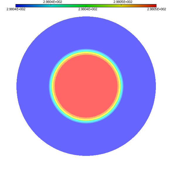
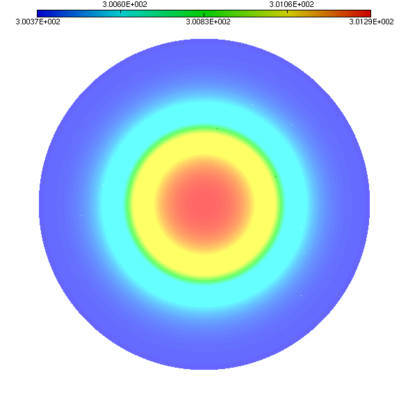
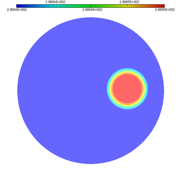
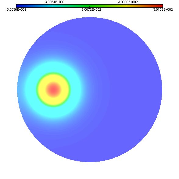
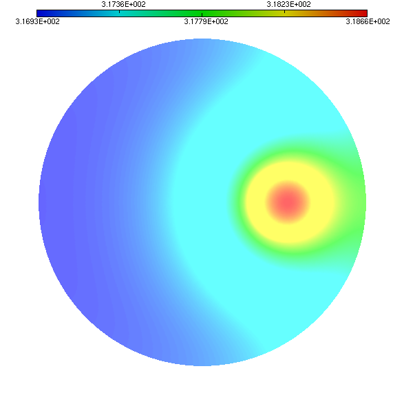
We perform two numerical experiments concerning the heat transfer process in 2D rotating disks with radius . The disks both consist of an aluminium circular area with radius and , respectively, and the complementary area filled by copper, see Figure 2. The domains are rotating with velocity and are partitioned into 245598 and 251536 triangles, respectively. Instead of the Joule heating , the system is supplied with a heat source . The changes over time of the temperature distribution are visualized by the software package MEDIT [12], which are shown in Figures 3 and 4.

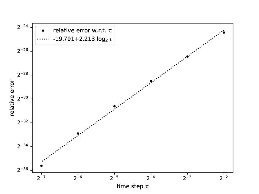
We verify the convergence of the temporal discretization scheme (18) in the time interval with . The reference temperature is the solution to (18) with time step , while larger time steps , with , are used to compute the discrete solution . Relative errors with respect to time step together with the corresponding regression lines are presented in Figure 5. The slope of the regression lines show that the potential convergence rate of the numerical scheme (18) is .
6.2. Numerical simulation
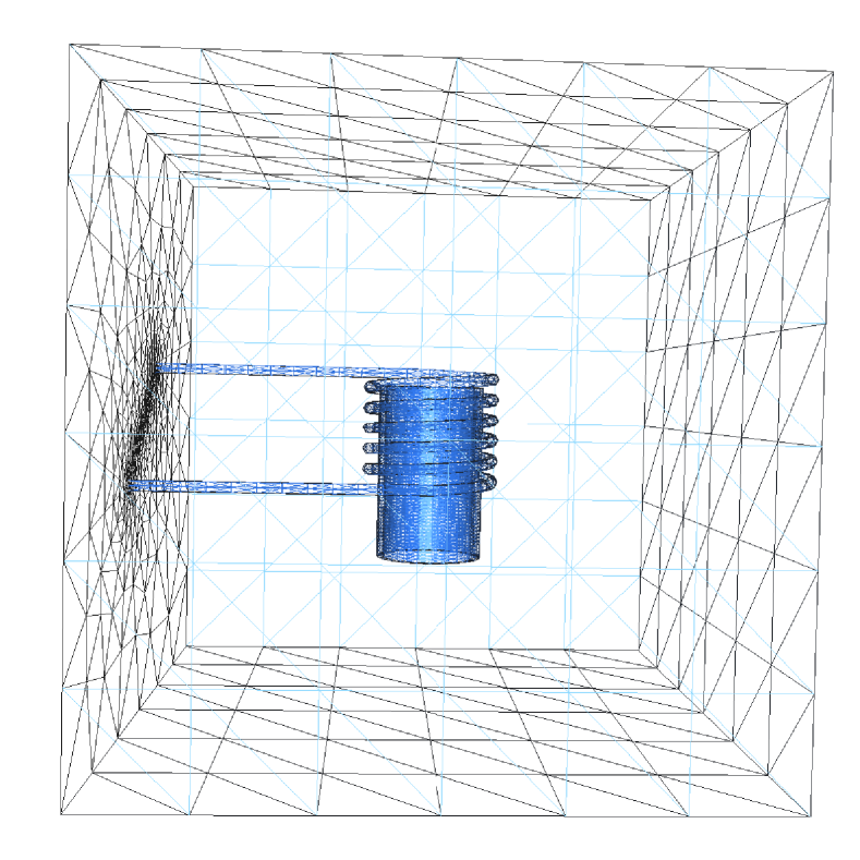
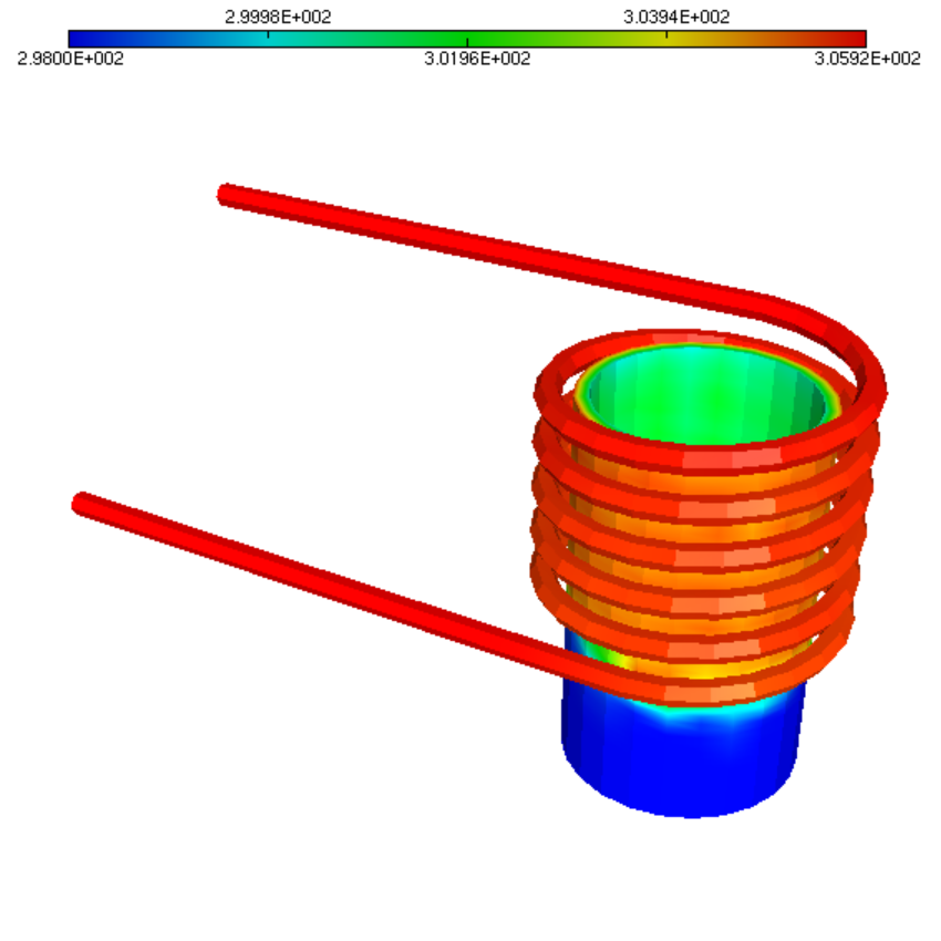
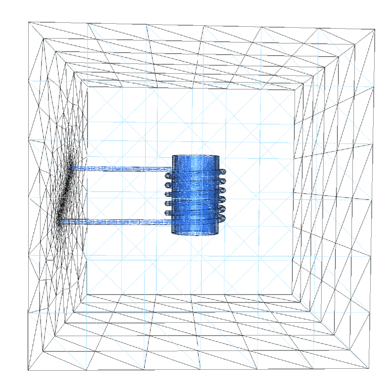
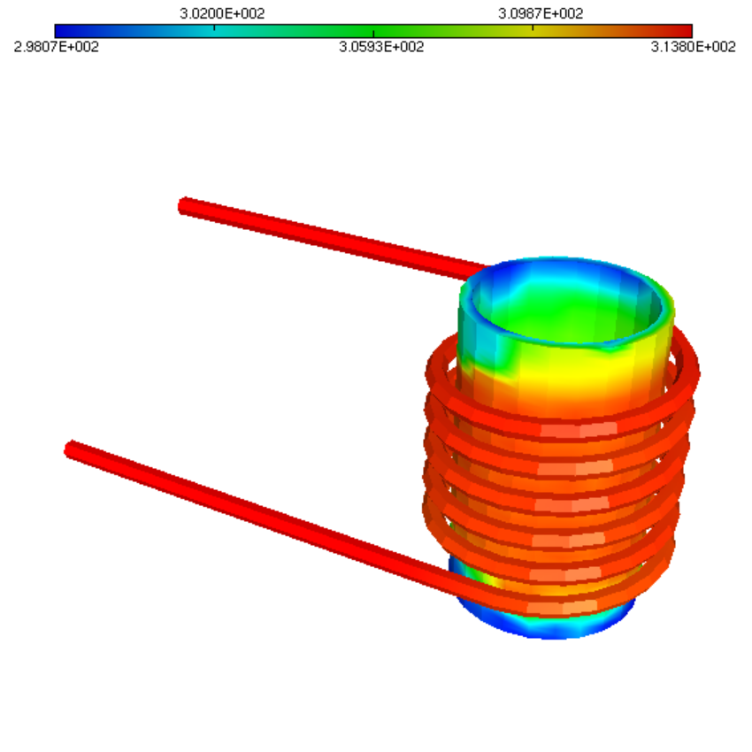
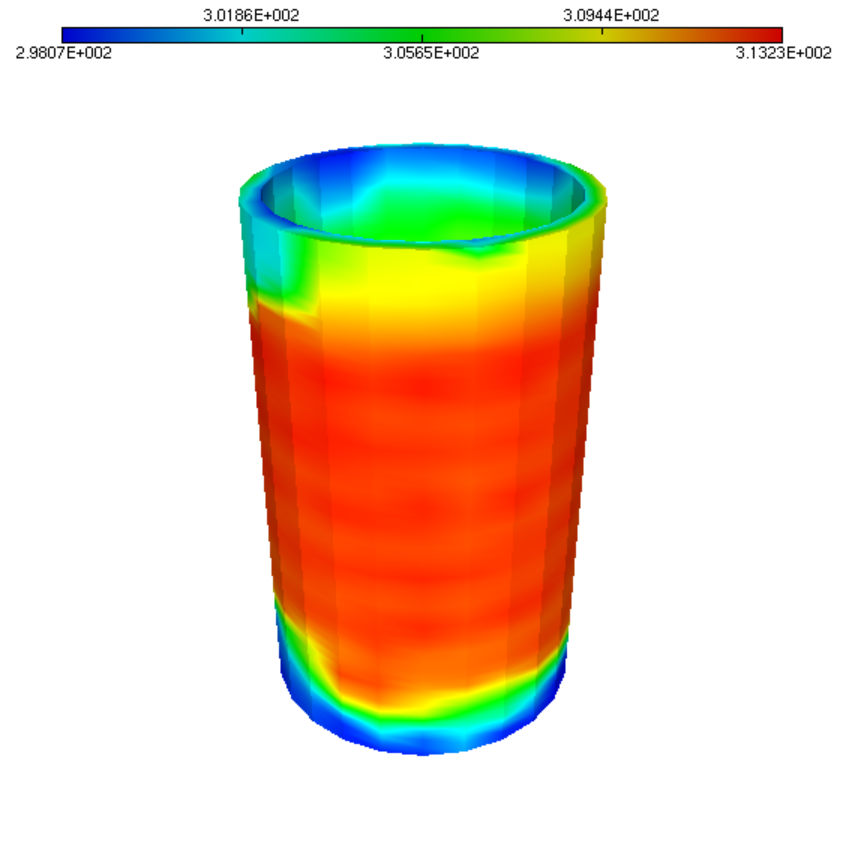
We enhance the numerical simulation of an induction heating process performed in [7] by considering a moving workpiece instead of a fixed one. The domain is a unit cube consisting of a thin-walled cylindrical aluminium workpiece with two radii and height , a copper coil and surrounding air. The initial guest on has a trivial extension on the whole domain without requiring regularity of the boundary of the subdomains and (see Remark 2.1). Hence, our theoretical results are still valid for this geometry. The domain is partitioned into tetrahedra. A static external current density with magnitude E7 is driven through the coil via the interfaces and . The workpiece is moving along the -axis with velocity , and the considered time length is . Outside the workpiece, we assume that the velocity is very small; thus, the thermal convection is dominated by the thermal conduction. Therefore, we can neglect the thermal convection effect in the air domain and avoid the computation of airflow, which is not essential in this paper.
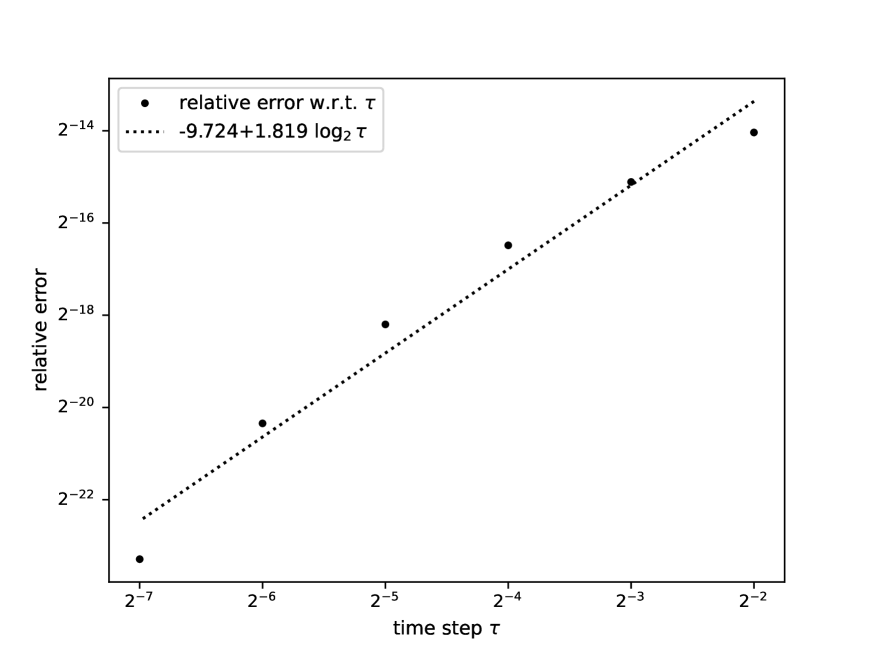
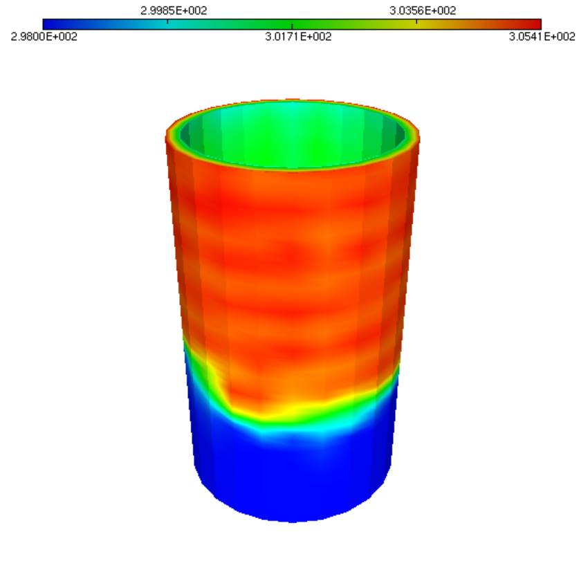
The reference solution is computed from the variational system (16)-(18) with time step ( subintervals). Different locations of the workpiece together with their corresponding temperature distributions on the conductors at two different time points are presented in Figure 6. Some rougher discrete solutions are also computed when the number of time intervals equals 64, 128, 256, 512, 1024 and 2048. Relative error with respect to time step and the corresponding regression line are shown in Figure 7, which confirms the potentially optimal convergence rate of our proposed scheme.

7. Conclusion
In the present paper, we have investigated an induction heating problem in a three-dimensional domain containing a moving non-magnetic conductor. The electromagnetic process and heat transfer are modelled by PDEs, which are coupled by the Joule heating effect. A cut-off function has been introduced to restrain the nonlinear Joule heat source. A time-discrete scheme based on the backward Euler’s method has been proposed to solve approximately the variational problems. The convergence of the proposed discretisation scheme and the well-posedness of the variational system have been proved with the aid of the Reynolds transport theorem and Rothe’s method. Some numerical results have also been presented to support the theoretical results.
In the future, comprehensive error estimates of the proposed temporal discretization scheme should be performed to verify the potentially optimal convergence rate obtained numerically in Section 6. In addition, future studies could concern high-frequency induction heating problems (full Maxwell’s equations) involving magnetic moving conductors, which have a wide range of applications in manufacturing industries.
References
- [1] X. Bai, H. Zhang, and G. Wang. Modeling of the moving induction heating used as secondary heat source in weld-based additive manufacturing. The International Journal of Advanced Manufacturing Technology, 77(1-4):717–727, 2014.
- [2] A. Bejan. Convection Heat Transfer. Wiley, fourth edition, 2013.
- [3] A. Bermúdez, B. López-Rodríguez, R. Rodríguez, and P. Salgado. Numerical solution of a transient three-dimensional eddy current model with moving conductors. International Journal of Numerical Analysis and Modeling, 16(5):695–717, 2019.
- [4] A. Bermúdez, R. Muñoz-Sola, C. Reales, R. Rodríguez, and P. Salgado. A Transient Eddy Current Problem on a Moving Domain. Mathematical Analysis. SIAM Journal on Mathematical Analysis, 45(6):3629–3650, 2013.
- [5] A. Bermúdez, C. Reales, R. Rodríguez, and P. Salgado. Numerical analysis of a transient eddy current axisymmetric problem involving velocity terms. Numerical Methods for Partial Differential Equations, 28(3):984–1012, 2011.
- [6] M. Bień. Existence of global weak solutions for a class of quasilinear equations describing Joule’s heating. Mathematical Methods in the Applied Sciences, 22(15):1275–1291, 1999.
- [7] J. Chovan, C. Geuzaine, and M. Slodička. A - formulation of a mathematical model for the induction hardening process with a nonlinear law for the magnetic field. Computer Methods in Applied Mechanics and Engineering, 321:294–315, 2017.
- [8] J. Chovan and M. Slodička. Induction hardening of steel with restrained Joule heating and nonlinear law for magnetic induction field: Solvability. Journal of Computational and Applied Mathematics, 311:630–644, 2017.
- [9] G. Di Fratta and A. Fiorenza. A short proof of local regularity of distributional solutions of Poisson’s equation. Proceedings of the American Mathematical Society, 148(5):2143–2148, 2020.
- [10] N. Di Luozzo, M. Fontana, and B. Arcondo. Modelling of induction heating of carbon steel tubes: Mathematical analysis, numerical simulation and validation. Journal of Alloys and Compounds, 536:S564–S568, 2012.
- [11] L. C. Evans. Partial Differential Equations, volume 19 of Graduate Studies in Mathematics. American Mathematical Society, 1997.
- [12] P. Frey. MEDIT: An interactive Mesh visualization Software. Technical report, INRIA, 2001.
- [13] V. Girault and P.-A. Raviart. Finite Element Methods for Navier-Stokes Equations: Theory and Algorithms, volume 5 of Springer Series in Computational Mathematics. Springer-Verlag, 1986.
- [14] M. Gurtin. An introduction to continuum mechanics, volume 158 of Mathematics in Science and Engineering. Academic Press, 1981.
- [15] F. Hecht. New development in freefem++. Journal of Numerical Mathematics, 20(3-4), 2012.
- [16] D. Hömberg. A mathematical model for induction hardening including mechanical effects. Nonlinear Analysis: Real World Applications, 5(1):55–90, 2004.
- [17] J. Kačur. Method of Rothe in Evolution Equations, volume 80 of Teubner-Text zur Mathematik. BSB B.G. Teubner Verlagsgesellschaft, 1985.
- [18] T. Kato, M. Mitrea, G. Ponce, and M. Taylor. Extension and Representation of Divergence-free Vector Fields on Bounded Domains. Mathematical Research Letters, 7(5):643–650, 2000.
- [19] V. C. Le. Advanced mathematical and numerical analysis of induction hardening of steel. PhD thesis, Ghent University, 2022.
- [20] V. C. Le, M. Slodička, and K. Van Bockstal. A time discrete scheme for an electromagnetic contact problem with moving conductor. Applied Mathematics and Computation, 404:125997, 2021.
- [21] V. C. Le, M. Slodička, and K. Van Bockstal. Error estimates for the time discretization of an electromagnetic contact problem with moving non-magnetic conductor. Computers & Mathematics with Applications, 87:27–40, 2021.
- [22] V. C. Le, M. Slodička, and K. Van Bockstal. A space-time discretization for an electromagnetic problem with moving non-magnetic conductor. Applied Numerical Mathematics, 173:345–364, 2022.
- [23] H.-P. Liu, X.-H. Wang, L.-Y. Si, and J. Gong. Numerical simulation of 3D electromagnetic-thermal phenomena in an induction heated slab. Journal of Iron and Steel Research International, 27(4):420–432, 2020.
- [24] R. A. Matula. Electrical resistivity of copper, gold, palladium, and silver. Journal of Physical and Chemical Reference Data, 8(4):1147–1298, 1979.
- [25] V. Rudnev, D. Loveless, and R. L. Cook. Handbook of Induction Heating. CRC Press, second edition, 2017.
- [26] R. A. Serway. Principles of Physics. Saunders College Pub., second edition, 1998.
- [27] H. Shokouhmand and S. Ghaffari. Thermal analysis of moving induction heating of a hollow cylinder with subsequent spray cooling: Effect of velocity, initial position of coil, and geometry. Applied Mathematical Modelling, 36(9):4304–4323, 2012.
- [28] M. Slodička and J. Chovan. Solvability for induction hardening including nonlinear magnetic field and controlled Joule heating. Applicable Analysis, 96(16):2780–2799, 2017.
- [29] M. Slodička. Parabolic problem for moving/ evolving body with perfect contact to neighborhood. Journal of Computational and Applied Mathematics, 391:113461, 2021.
- [30] Y.-S. Touloukian, R.-W. Powell, C.-Y. Ho, and P.-G. Klemens. Thermophysical properties of matter - the TPRC Data Series. Purdue Research Foundation, 1970.
- [31] Z. Wang, W. Huang, W. Jia, Q. Zhao, Y. Wang, W. Yan, D. Schulze, G. Martin, and U. Luedtke. 3D Multifields FEM Computation of Transverse Flux Induction Heating for Moving-Strips. IEEE Transactions on Magnetics, 35:1642–1645, 1999.
- [32] H. Wen and Y. Han. Study on mobile induction heating process of internal gear rings for wind power generation. Applied Thermal Engineering, 112:507–515, 2017.
- [33] H.-M. Yin. Global solutions of Maxwell’s equations in an electromagnetic field with a temperature-dependent electrical conductivity. European Journal of Applied Mathematics, 5(1):57–64, 1994.
- [34] H.-M. Yin. Regularity of solutions to Maxwell’s system in quasi-stationary. Communications in Partial Differential Equations, 22(7-8):57–64, 1997.
- [35] H.-M. Yin. On Maxwell’s Equations in an Electromagnetic Field with the Temperature Effect. SIAM Journal on Mathematical Analysis, 29:637–651, 1998.
- [36] A. Zabett and S. H. Mohamadi Azghandi. Simulation of induction tempering process of carbon steel using finite element method. Materials & Design (1980-2015), 36:415–420, 2012.
- [37] E. Zeidler. Nonlinear Functional Analysis and Its Applications. Part II/A: Linear Monotone Operators. Springer-Verlag, 1990.