Analysis of a subsolar-mass compact binary candidate
from the second observing run of Advanced LIGO
Abstract
We perform an exhaustive follow-up analysis of a subsolar-mass (SSM) gravitational wave (GW) candidate reported by Phukon et al. from the second observing run of Advanced LIGO. This candidate has a reported signal-to-noise ratio (SNR) of and false alarm rate of yr which are too low to claim a clear gravitational-wave origin. When improving on the search by using more accurate waveforms, extending the frequency range from 45 Hz down to 20 Hz, and removing a prominent blip glitch, we find that the posterior distribution of the network SNR lies mostly below the search value, with the 90% confidence interval being . Assuming that the origin of the signal is a compact binary coalescence (CBC), the secondary component is , with at confidence level, suggesting an unexpectedly light neutron star or a black hole of primordial or exotic origin. The primary mass would be , likely in the hypothesized lower mass gap and the luminosity distance is measured to be Mpc. We then probe the CBC origin hypothesis by performing the signal coherence tests, obtaining a log Bayes factor of for the coherent vs. incoherent hypothesis. We demonstrate the capability of performing a parameter estimation follow-up on real data for an SSM candidate with moderate SNR. The improved sensitivity of O4 and subsequent LIGO-Virgo-KAGRA observing runs could make it possible to observe similar signals, if present, with a higher SNR and more precise measurement of the parameters of the binary.
I Introduction
The development of gravitational wave astronomy, with about 90 compact binary coalescence (CBC) events detected so far Abbott et al. (2016a, b, 2019a, 2021a, 2021b, 2021c) by the LIGO-Virgo-KAGRA (LVK) collaboration Abbott et al. (2020a), is driving a true revolution in astrophysics and cosmology. As the number of detected events grows with successive observing catalogs, the range of the inferred component masses has extended to previously unexplored regions, with black holes (BH) found Abbott et al. (2020b, c) in the pair-instability mass gap Woosley (2017) and in the hypothesized lower mass gap Abbott et al. (2020d). The frequency range of the LIGO Collaboration et al. (2015) and Virgo Acernese et al. (2014) detectors makes them also sensitive to CBC signals in which one of the compact objects has a mass below 1. The detection of a sub-solar mass (SSM) compact object would be of utmost interest since it would require either modification of the standard astrophysical evolution and collapse of ordinary matter or a new formation mechanism operating in the Universe, such as primordial black holes (PBHs) Zel’dovich and Novikov (1967); Hawking (1971); Carr and Hawking (1974); Chapline (1975); García-Bellido et al. (1996) or SSM objects originated by dark matter with exotic properties Kouvaris and Tinyakov (2011); de Lavallaz and Fairbairn (2010); Bramante and Linden (2014); Bramante and Elahi (2015); Bramante et al. (2018); Kouvaris et al. (2018); Shandera et al. (2018); Chang et al. (2019); Latif et al. (2019); Dasgupta et al. (2021); Gurian et al. (2022); Ryan and Radice (2022); Hippert et al. (2022).
Before the advent of GW astronomy, the only way to detect SSM black holes was via X-ray binaries Corral-Santana et al. (2016) or microlensing Paczynski (1986). At present, some hints of the existence of such light black holes come from microlensing events towards the bulge Wyrzykowski and Mandel (2020), from Andromeda Niikura et al. (2019) and lensed quasars Hawkins (2020, 2022), although the mass and the abundance of the lenses remain uncertain. Complementary to these astrophysical searches, GW signals of CBC with at least one subsolar component have been searched for in the first (O1), second (O2) and third (O3) observing runs of LVK Abbott et al. (2018a, 2019b); Nitz and Wang (2021a); Abbott et al. (2022a, b), without finding compelling evidence for a clear detection. Nevertheless, a further search in the O2 data for SSM black holes with low mass ratios Phukon et al. (2021) and the latest O3b SSM search results from LVK Abbott et al. (2022b) have reported several potential candidates with a false alarm rate smaller than .
In this work, we follow up on the O2 search reported in Phukon et al. (2021), using the standard parameter estimation (PE) methods to further investigate the candidates reported in Table I. Given that PE on these long GW signals is extremely time consuming, we have focused on the third candidate of the table, which is the lowest FAR trigger found in coincidence by both LIGO Hanford and LIGO Livingston interferometers, which allows more confident rejection against terrestrial noise. This candidate was observed on April 1st 2017 and we will refer to it here as SSM170401.
In this analysis we have extended the frequency range of the search from 45 Hz down to 20 Hz. We have also improved upon the TaylorF2 Buonanno et al. (2009) waveform used in the template bank of search, by using for PE the more accurate waveforms IMRPhenomPv2 Hannam et al. (2014) and IMRPhenomXPHM Pratten et al. (2021) that include the merger and ringdown phases, as well as spin precession and, in the case of IMRPhenomXPHM, higher order modes. We have also inspected the quality of the data and discussed the impact of a prominent glitch removal using standard tools such as BayesWave Cornish and Littenberg (2015); Littenberg and Cornish (2015); Davis et al. (2022). Finally, assuming that the origin of the candidate is a BBH merger, the PE allows us to infer the component masses, spins, distance and sky location, as well as the posterior probability of having an SSM component of the hypothetical source for SSM170401.
In the following sections, we describe in detail different aspects of this analysis that reveal the peculiarities and difficulties of doing PE on this type of candidate, as well as the necessary analysis tools in preparation for a possible future significant candidate, given the increase of sensitivity expected in the O4 run.
II Significance of SSM170401
The candidate was found in data taken on April 1st, 2017, 01:43:34 UTC during the O2 LIGO-Virgo observing run. It was not reported by any of the LVK searches, both generic Abbott et al. (2019a) and SSM specific Abbott et al. (2019c), but it was found in a dedicated search for SSM mergers in asymmetric binaries using the GstLAL pipeline Phukon et al. (2021). The search reported detector frame masses of 4.897 and 0.7795 , with a false-alarm-rate (FAR) of 0.4134 yr-1 and a combined network signal-to-noise ratio (SNR) of . Given that the time of O2 coincident data suitable for observation is Abbott et al. (2019a), the false alarm probability (FAP) of this candidate, according to the search is:
| (1) |
The interpretation of this FAP is that the search would produce a higher-ranked candidate in 12% of trials over data containing only noise.
We can also estimate an upper bound for the probability of this signal coming from a CBC merger with an SSM component, given the upper limits on event rates obtained from the O3 SSM searches. Abbott et al. (2022a, b). In Ref. Abbott et al. (2022b) the 90 C.L. constraints on the merger rate of SSM binaries are reported in the plane, assuming null results of these searches. For the median values of the component masses of the source of SSM170411 (see Table 1), we find . Moreover, in the search where the signal was identified Phukon et al. (2021), the volume-time surveyed for these same masses is reported to be . Since the arrival of GWs from binary mergers to the detectors is Poisson distributed, with an expected number of events , the probability of finding events would be:
| (2) |
Using the values previously mentioned for and , the upper bound on the expected number of events is at C.L. and the corresponding upper bound on the probability for the search in Ref. Phukon et al. (2021) to have found one or more events would be smaller than . Therefore, the results of O3 do not particularly constrain the possibility that SSM170401 could come from a real SSM merger.
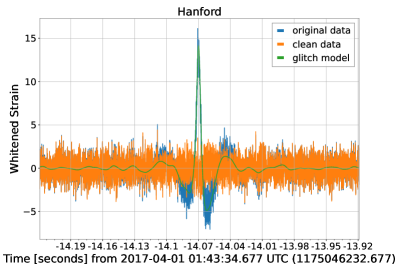
The strain in Hanford presents a glitch 14 s before coalescence, as shown in Fig. 1. The search presented in Ref. Phukon et al. (2021) uses templates starting at 45 Hz. The loudest template, in this case, is only 10 s long and so should be unaffected by the glitch. However, PE was performed with templates starting at 20 Hz, which are roughly 100 s long for the component masses discussed. In this situation the glitch must be removed. Using BayesWave Cornish and Littenberg (2015); Littenberg and Cornish (2015), we model excess power in the detectors as a sum of sine-Gaussian wavelets. We fit for the glitch and the PSD of the Gaussian noise component simultaneously. We ignore the modelling of the signal due to the extremely low coherent energy per frequency bin deposited in the detectors in the 0.3 s duration of the glitch by such low mass sources, even more when the subtraction is done s before coalescence. The same procedure is used routinely by the LVK collaboration in the main GW catalog Abbott et al. (2021c).
III Properties of the source of SSM170401
To obtain the properties of the potential source of SSM170401 we interpret the signal as coming from the coalescence of two compact objects. We infer the CBC parameters of the signal using a Bayesian analysis of the data from LIGO Livingston and LIGO Hanford, following the methodology outlined in Appendix B of Ref. Abbott et al. (2019a). In analysing the data, we fit two different waveform models: IMRPhenomPv2 Hannam et al. (2014) and IMRPhenomXPHM Pratten et al. (2021), the latter including higher order modes. Comparing the PE analyses using the two waveforms models, we find that their posterior distributions are consistent with each other, noting that both of them take into account precessing spins.
| Parameter | IMRPhenomPv2 | IMRPhenomXPHM |
|---|---|---|
| Signal to Noise Ratio | ||
| Primary mass () | ||
| Secondary mass () | ||
| Primary spin magnitude | ||
| Secondary spin magnitude | ||
| Total mass () | ||
| Mass ratio | ||
| Ajith et al. (2011); Santamaría et al. (2010) | ||
| Schmidt et al. (2015) | ||
| Luminosity Distance (Mpc) | ||
| Redshift | ||
| Ra (∘) | ||
| Dec (∘) | ||
| Final mass () | ||
| Final spin | ||
We use a low-frequency cutoff of 20 Hz in both detectors for the likelihood evaluation and choose uninformative and wide priors. The primary tool used for sampling the posterior distribution is the LALInference Markov Chain Monte Carlo implementation as described in Veitch et al. (2015). The power spectral density used in the calculations of the likelihood is estimated using BayesWave Cornish and Littenberg (2015); Littenberg and Cornish (2015). The study uses the O2 open access data Abbott et al. (2021d) with a sampling frequency of 4096 Hz; however the likelihood is integrated up to 1600 Hz.
The best fit CBC template has 3000 cycles in the detector, allowing us to constrain with relatively high accuracy the source properties of SSM170401 in spite of the low SNR Cutler et al. (1993). The estimated parameters are reported in Table 1. The marginalized posterior for the absolute value of the matched filter SNR is for IMRPhenomPv2 and for IMRPhenomXPHM. The median value of the SNR is lower than that found by the search, which was . However, these two quantities are not directly comparable. The SNR from the search is obtained by maximizing the ranking statistic over a discrete template bank Phukon et al. (2021); Messick et al. (2017); Cannon et al. (2012, 2021), while the quoted SNR from the PE is the median value over the samples. Since the ranking statistic and the SNR are closely related, the SNR that is more comparable to that of the search would be the maximum SNR as found by the PE. The values of this maximum PE SNR are for IMRPhenomPv2 and for IMRPhenomXPHM. These values are slightly larger than that of the search, which is consistent with what would happen if the signal was astrophysical. However, this is also expected in the noise case due to the larger parameter space that allows more flexibility for the PE analysis to fit the data. We also notice the maximum value of the SNR to be larger for IMRPhenomXPHM than for IMRPhenomPv2. In a similar way, this is expected for an astrophysical signal but also for noise, since the waveform includes Higher Order Modes and thus has more flexibility to fit the data.
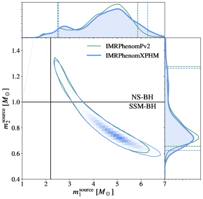
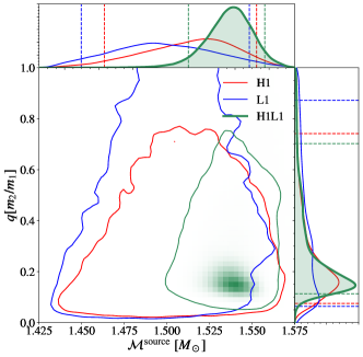
The source is then compatible with a compact binary system having an unequal mass ratio (all uncertainties are quoted at 90% C.L.), a source frame primary mass and a source frame secondary mass as shown in Fig. 2. The marginalised posterior distribution for the secondary mass favors a mass lower than ( C.L.). Using the IMRPhenomXPHM waveform, we find almost identical results, with a mass lower than at C.L.
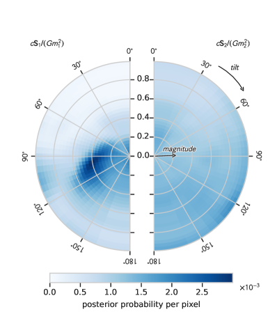
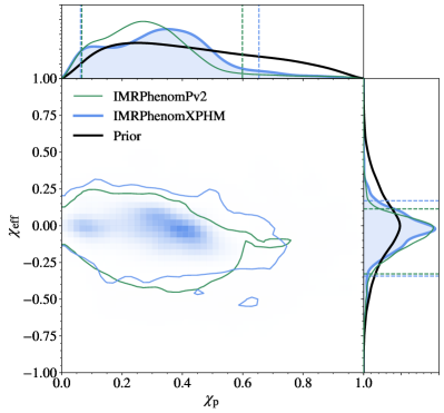
The left panel of Fig. 3 shows the posterior distributions for the magnitude and tilt angle of the individual spins, measured at a reference frequency of 20 Hz. All pixels in this plot have an equal prior probability. The spin of the secondary BH is largely unconstrained, as expected for very unequal masses, while the primary spin shows a preference for small spin magnitudes (), where the posterior samples with large primary spin tend to have it misaligned with the orbital angular momentum. As can be seen in the right panel of Fig. 3, this leads to a compatible with zero () and an uninformative posterior in ().
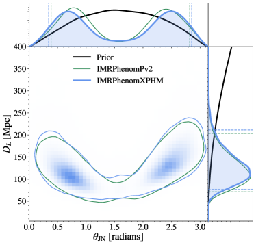
The luminosity distance and inclination angle posterior distributions are shown together in the left panel of Fig. 4, since these two quantities are correlated. We find a luminosity distance of Mpc. We identify a bimodal distribution for due to the fact that we can not distinguish whether the system is being observed face-on () or face-away (), but it being edge-on () is disfavoured. In the face-on(away) configuration, the effects of precession and higher order modes in the signal are suppressed Krishnendu and Ohme (2022); Calderón Bustillo et al. (2017); Mills and Fairhurst (2021), as is the case here.
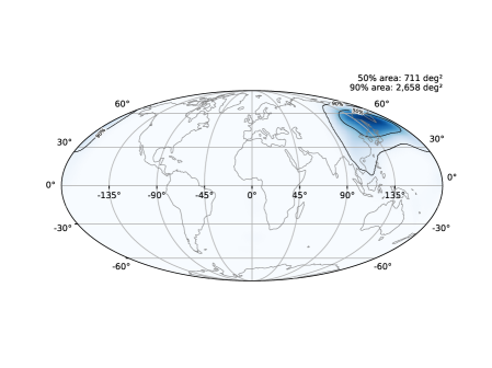
In the right panel of Fig. 4, we show the posterior distribution of the location in the sky of the event. This sky map looks abnormal when compared with the typical ones of the events detected exclusively by Hanford and Livingston Abbott et al. (2019a, 2021a, 2021b, 2021c). When the trigger is seen in two detectors only, most of the information for the sky localisation comes from the time delay between the observation of the signal in both interferometers. This time delay will be given by:
| (3) |
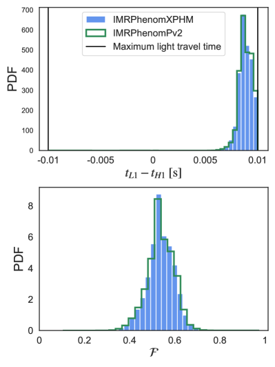
where is the position vector of Livingston with respect to Hanford and is the direction in the sky of the source. We observe in Eq. (3) that the time delay only constraints the inclination angle with respect to , but leaves the azimuthal angle completely unconstrained. This has as a result a ring-like shape in the sky maps usually observed. However, when the source direction corresponds to , that is, the line joining both detectors, the ring will collapse to have a blob like shape in the sky. As can be seen in the top panel of Figure 5, this is what is happening for the source of SSM170401, since the time delay between Livingston and Hanford is close to the maximum light travel time. In the bottom panel of Figure 5 we also show the posterior distribution of the network antenna pattern Klimenko et al. (2011), defined as:
| (4) |
where are the () antenna patterns of detector . In this plot we observe that the event is coming from a region in the sky where the network antenna pattern is significantly smaller than 1, peaking at . This means that the sensitivity in this direction will be half of that of the most sensitive direction () located on top of the continental US and its antipodes Andersson et al. (2013). Since the direction joining both LIGO detectors has smaller sensitivity, the distance up to which LIGO can detect astrophysical signals is also smaller. This leads to a lower expected event rate coming from that direction, which is the reason sky maps like the one of Fig. 4 are uncommon.
Even though the posterior PDFs for the parameters of the source of SSM170401 seem to have converged to a well-defined distribution that differs from the prior, it is known that GW signals can be mimicked by gaussian noise Morras et al. (2023) or non-gaussian transients, specially given the relatively low SNR and high FAR.
III.1 Coherence Test
To test the compatibility of the SSM170401 with a GW coming from a CBC, we perform the coherence test proposed in Ref. Veitch and Vecchio (2010). The idea of this test is to perform Bayesian PE using the data from all the detectors together to calculate the evidence for a coherent CBC signal and compare this with the evidence for incoherent CBC signals. The incoherent evidence is defined as the product of the CBC signal evidences obtained performing PE individually in each detector. These incoherent CBC signals are used to represent noise in the detectors that can be picked up by CBC templates. The coherent versus incoherent hypothesis Bayes factor is then defined as
| (5) |
where we have used that for each interferometer, the Bayes factor of the signal versus noise hypothesis is defined as , while in the coherent analysis it is defined as . We use the same priors for coherent and single-detector analyses. To get a more reliable estimate of the evidence, in the PE we use nested sampling, particularly the Dynesty sampler Speagle (2020) as implemented in Bilby Ashton et al. (2019). The computational cost of performing the coherence test will be very large since it requires us to perform three separate PEs with the costly nested sampling. To make this analysis feasible we employ Reduced Order Quadrature (ROQ) methods Smith et al. (2016), which greatly speed up the computation time of the likelihood, specially for long signals like SSM170401. The analysis is done using only the IMRPhenomPv2 waveform, since we have seen that it gives consistent results with IMRPhenomXPHM while leading to much greater ROQ speedups Qi and Raymond (2021). We obtain the Bayes factors listed in Table. 2. We find a value for , strongly favoring the coherent hypothesis over the incoherent hypothesis Trotta (2008).
This result, however, cannot be used to update the statistical significance of the candidate since we have not run the coherence test over the background triggers of the search. While it is unlikely that a randomly selected noise candidate would give such a large value of Isi et al. (2018), we note that the search ranking promotes candidates with parameters consistent between different detectors Cannon et al. (2015), thus it may be less surprising that a highly ranked candidate has large . In Fig. 6 we also show the posterior distributions of obtained performing PE in each detector individually and coherently in both of them. We observe that the 2D contours are compatible with each other, having larger areas in the single-detector analyses. This behavior is what is expected if the signal in both detectors were generated by the GWs coming from a single CBC Veitch and Vecchio (2010).
IV Discussion
To discuss the possible source of SSM170401, assuming it is a CBC, we have divided the in four regions, according to the SSM threshold () and the maximum allowed mass of a NS () Margalit and Metzger (2017); Ruiz et al. (2018); Cromartie et al. (2019). We observe that the full credible region of the posterior lies in the region of , excluding the NS origin of the primary component. We find that of the posterior distribution lies in the region of , which would point to a likely NS origin, although a light black hole cannot be excluded. However, the most probable region, representing of the posterior, would imply a mass of the secondary component below . It is thus interesting to explore what could be the origin and nature of a possible SSM object.
The first possibility to consider for an SSM component would be a neutron star. Neutron stars have relatively well-determined masses from observations of binary systems, including pulsars or X-ray binaries involving an accreting neutron star from a companion. Their measured masses are above Lattimer (2019), further confirmed by the observation of GW170817 Abbott et al. (2017). However, there is a recent claim Doroshenko et al. (2022) for a neutron star of mass , although it has been argued Sotani et al. (2014) that such a small mass for a neutron star probably requires a strange QCD equation of state. Therefore, the neutron star interpretation of a possible SSM component cannot be excluded, although it is disfavored by the bulk of observational data.
Another possibility is PBHs formed by the gravitational collapse of large inhomogeneities in the early Universe which are already considered as a possible explanation of LVK GW detections, see e.g. Bird et al. (2016); Clesse and García-Bellido (2017); Sasaki et al. (2016); Clesse and García-Bellido (2018); Fernandez and Profumo (2019); Carr et al. (2021); Jedamzik (2020, 2021); Clesse and García-Bellido (2022); Fernandez and Profumo (2019); Hütsi et al. (2021); Hall et al. (2020); García-Bellido et al. (2021); Franciolini et al. (2021). Depending on the model, they may explain anything from a tiny fraction of Dark Matter to its entirety. PBHs have been the main motivation to conduct searches of SSM black holes in the LVK data Abbott et al. (2018b, 2019c); Nitz and Wang (2021b); Phukon et al. (2021); Nitz and Wang (2021a); Abbott et al. (2022a); Nitz and Wang (2022), in particular, the extended subsolar search with low-mass ratios in O2 which reported SSM170401 as a possible candidate Phukon et al. (2021). If some of the observed binary coalescences are indeed due to PBHs, they must have a relatively extended mass distribution that would have been imprinted by the thermal history of the Universe Byrnes et al. (2018); Carr et al. (2021). This would lead to a peak in the mass distribution around a solar mass which is naturally produced at the QCD transition Jedamzik (1997); Niemeyer and Jedamzik (1998); Byrnes et al. (2018); Carr et al. (2021); Garcia-Bellido et al. (2021); Escrivà et al. (2022); Franciolini et al. (2022), and the source of SSM170401 could be an example of a subsolar PBH around the QCD-induced peak. The spin posterior is quite broad and the spin is compatible with zero, although a slight preference for a primary spin around 0.3 is observed. In this case, the non-zero but relatively low spin of the primary component may have been acquired by matter accretion, previous mergers or hyperbolic encounters De Luca et al. (2020); García-Bellido et al. (2021); Jaraba and García-Bellido (2021).
Alternatively, in scenarios with complex and dissipative particle Dark Matter, SSM black holes could form through the cooling and gravitational collapse of Dark Matter halos Shandera et al. (2018). This model was constrained by the LVK data in Singh et al. (2021); Abbott et al. (2022a, c). Furthermore, it could be that the secondary component of the source of SSM170401 is a boson star, a hypothetical horizonless compact object formed by an ultralight bosonic field. If the mass of the bosonic particle is larger than , the boson star can have subsolar mass Liebling and Palenzuela (2012). Whether a merger with an SSM boson star component could produce a signal similar to the SSM170401 trigger, though, remains to be investigated.
Finally, we note that the primary component mass of the hypothetical source of SSM170401 would preferably lie in the hypothesized low mass gap between and (C.L.). However, this is not unique, since other candidates with components possibly in this lower mass gap have been observed, namely GW190814 Abbott et al. (2020d) and GW200210-092254 Abbott et al. (2021c).
V Conclusions
We have performed an in-depth investigation of the most significant double-detector candidate reported in Phukon et al. (2021) in an SSM search over O2 data. We have removed a prominent blip glitch 14 s before coalescence in the data and estimated the parameters of the possible CBC source using a low frequency cutoff of 20 Hz. Parameter Estimation runs were performed using LALInference with two different waveforms IMRPhenomPv2 and IMRPhenomXPHM, where the latter includes effects from higher order modes. The source parameters obtained by both PE runs show good agreement with each other and with the parameters of the template that triggered the search. We find a median network SNR of ( credible interval), which is lower than the SNR of obtained in the search. However, the search SNR is more closely related to the maximum SNR, which we find to be higher in the PE, where it reaches values of for IMRPhenomPv2 and for IMRPhenomXPHM. The secondary mass is ( credible interval), with confidence of being below one solar mass. For the location in the sky posterior, we find an atypical distribution when compared with the usual Hanford-Livingston events detected thus far, which can be explained if it were a GW coming from the direction joining the two LIGO interferometers.
The compatibility of SSM170401 with a CBC origin has been further tested by performing the signal coherence tests of Ref Veitch and Vecchio (2010), obtaining a log Bayes factor of for the coherent vs incoherent hypothesis. Furthermore, we observe that the posteriors of each independent IFO converge to mutually compatible contours. These tests provide significant support in favor of a coherent signal, which generally is not expected if it were generated by noise fluctuations Isi et al. (2018). We also checked that the O3 limits on the SSM merger rate Abbott et al. (2022c) do not put a significant constraint on the probability of this candidate being astrophysical (). Therefore, we do not find compelling arguments against a possible CBC origin of SSM170401.
Finally, even if most of the posterior support is in the SSM region, there is still a probability of being over 1 , which does not allow us to convincingly exclude a NS origin. Candidates with a higher SNR would have better measurements on their parameters, allowing for more confident discrimination between sub- and super- solar masses Wolfe et al. (2023). Therefore, the data from future planned LIGO-Virgo-Kagra runs with improved sensitivity Abbott et al. (2020a), O4 and O5, offer a great opportunity for discovering CBC mergers with SSM components, if they are out there in the Cosmos.
Acknowledgements.
The authors thank Patrick Meyers and Walter Del Pozzo for their helpful comments and discussions as reviewers of this paper in LIGO and Virgo respectively as well as Juan Calderón Bustillo and Geraint Pratten for their constructive feedback. We thank the anonymous referee for their careful reading of our manuscript and their many insightful comments and suggestions. This work is partially supported by the Spanish grants PID2020-113701GB-I00, PID2021-123012NB-C43 [MICINN-FEDER], and the Centro de Excelencia Severo Ochoa Program CEX2020-001007-S through IFT, some of which include ERDF funds from the European Union. S.C. acknowledges support from the Francqui Foundation through a Starting Grant. K.M. is supported by King’s College London through a Postgraduate International Scholarship. M.S. is supported in part by the Science and Technology Facility Council (STFC), United Kingdom, under the research grant ST/P000258/1. IFAE is partially funded by the CERCA program of the Generalitat de Catalunya. We acknowledge the use of IUCAA LDG cluster Sarathi for the computational/numerical work. This material is based upon work supported by NSF’s LIGO Laboratory which is a major facility fully funded by the National Science Foundation.References
- Abbott et al. (2016a) B. P. Abbott et al. (LIGO Scientific, Virgo), Phys. Rev. Lett. 116, 061102 (2016a), arXiv:1602.03837 [gr-qc] .
- Abbott et al. (2016b) B. P. Abbott et al. (LIGO Scientific, Virgo), Phys. Rev. X 6, 041015 (2016b), [Erratum: Phys.Rev.X 8, 039903 (2018)], arXiv:1606.04856 [gr-qc] .
- Abbott et al. (2019a) B. P. Abbott et al. (LIGO Scientific, Virgo), Phys. Rev. X 9, 031040 (2019a), arXiv:1811.12907 [astro-ph.HE] .
- Abbott et al. (2021a) R. Abbott et al. (LIGO Scientific, Virgo), Phys. Rev. X 11, 021053 (2021a), arXiv:2010.14527 [gr-qc] .
- Abbott et al. (2021b) R. Abbott et al. (LIGO Scientific, VIRGO), (2021b), arXiv:2108.01045 [gr-qc] .
- Abbott et al. (2021c) R. Abbott et al. (LIGO Scientific, Virgo, KAGRA), (2021c), arXiv:2111.03606 [gr-qc] .
- Abbott et al. (2020a) B. Abbott, R. Abbott, T. Abbott, S. Abraham, F. Acernese, K. Ackley, C. Adams, V. Adya, C. Affeldt, M. Agathos, K. Agatsuma, N. Aggarwal, O. Aguiar, L. Aiello, A. Ain, P. Ajith, T. Akutsu, G. Allen, and A. Allocca, Living Reviews in Relativity 23 (2020a), 10.1007/s41114-020-00026-9.
- Abbott et al. (2020b) R. Abbott et al. (LIGO Scientific, Virgo), Phys. Rev. Lett. 125, 101102 (2020b), arXiv:2009.01075 [gr-qc] .
- Abbott et al. (2020c) R. Abbott et al. (LIGO Scientific, Virgo), Astrophys. J. Lett. 900, L13 (2020c), arXiv:2009.01190 [astro-ph.HE] .
- Woosley (2017) S. E. Woosley, Astrophys. J. 836, 244 (2017), arXiv:1608.08939 [astro-ph.HE] .
- Abbott et al. (2020d) R. Abbott et al. (LIGO Scientific, Virgo), Astrophys. J. 896, L44 (2020d), arXiv:2006.12611 [astro-ph.HE] .
- Collaboration et al. (2015) T. L. S. Collaboration, J. Aasi, B. P. Abbott, R. Abbott, et al., Classical and Quantum Gravity 32, 074001 (2015).
- Acernese et al. (2014) F. Acernese, M. Agathos, et al., Classical and Quantum Gravity 32, 024001 (2014).
- Zel’dovich and Novikov (1967) Y. B. Zel’dovich and I. D. Novikov, Soviet Astronomy 10, 602 (1967).
- Hawking (1971) S. Hawking, Mon. Not. Roy. Astron. Soc. 152, 75 (1971).
- Carr and Hawking (1974) B. J. Carr and S. W. Hawking, Mon. Not. Roy. Astron. Soc. 168, 399 (1974).
- Chapline (1975) G. F. Chapline, Nature 253, 251 (1975).
- García-Bellido et al. (1996) J. García-Bellido, A. D. Linde, and D. Wands, Phys. Rev. D 54, 6040 (1996), arXiv:astro-ph/9605094 .
- Kouvaris and Tinyakov (2011) C. Kouvaris and P. Tinyakov, Phys. Rev. D 83, 083512 (2011), arXiv:1012.2039 [astro-ph.HE] .
- de Lavallaz and Fairbairn (2010) A. de Lavallaz and M. Fairbairn, Phys. Rev. D 81, 123521 (2010), arXiv:1004.0629 [astro-ph.GA] .
- Bramante and Linden (2014) J. Bramante and T. Linden, Phys. Rev. Lett. 113, 191301 (2014), arXiv:1405.1031 [astro-ph.HE] .
- Bramante and Elahi (2015) J. Bramante and F. Elahi, Phys. Rev. D 91, 115001 (2015), arXiv:1504.04019 [hep-ph] .
- Bramante et al. (2018) J. Bramante, T. Linden, and Y.-D. Tsai, Phys. Rev. D 97, 055016 (2018), arXiv:1706.00001 [hep-ph] .
- Kouvaris et al. (2018) C. Kouvaris, P. Tinyakov, and M. H. G. Tytgat, Phys. Rev. Lett. 121, 221102 (2018), arXiv:1804.06740 [astro-ph.HE] .
- Shandera et al. (2018) S. Shandera, D. Jeong, and H. S. G. Gebhardt, Phys. Rev. Lett. 120, 241102 (2018), arXiv:1802.08206 [astro-ph.CO] .
- Chang et al. (2019) J. H. Chang, D. Egana-Ugrinovic, R. Essig, and C. Kouvaris, JCAP 03, 036 (2019), arXiv:1812.07000 [hep-ph] .
- Latif et al. (2019) M. A. Latif, A. Lupi, D. R. G. Schleicher, G. D’Amico, P. Panci, and S. Bovino, Mon. Not. Roy. Astron. Soc. 485, 3352 (2019), arXiv:1812.03104 [astro-ph.CO] .
- Dasgupta et al. (2021) B. Dasgupta, R. Laha, and A. Ray, Phys. Rev. Lett. 126, 141105 (2021), arXiv:2009.01825 [astro-ph.HE] .
- Gurian et al. (2022) J. Gurian, M. Ryan, S. Schon, D. Jeong, and S. Shandera, Astrophys. J. Lett. 939, L12 (2022), arXiv:2209.00064 [astro-ph.CO] .
- Ryan and Radice (2022) M. Ryan and D. Radice, Phys. Rev. D 105, 115034 (2022), arXiv:2201.05626 [astro-ph.HE] .
- Hippert et al. (2022) M. Hippert, E. Dillingham, H. Tan, D. Curtin, J. Noronha-Hostler, and N. Yunes, (2022), arXiv:2211.08590 [astro-ph.HE] .
- Corral-Santana et al. (2016) J. M. Corral-Santana, J. Casares, T. Munoz-Darias, F. E. Bauer, I. G. Martinez-Pais, and D. M. Russell, Astron. Astrophys. 587, A61 (2016), arXiv:1510.08869 [astro-ph.HE] .
- Paczynski (1986) B. Paczynski, Astrophys. J. 304, 1 (1986).
- Wyrzykowski and Mandel (2020) Ł. Wyrzykowski and I. Mandel, Astron. Astrophys. 636, A20 (2020), arXiv:1904.07789 [astro-ph.SR] .
- Niikura et al. (2019) H. Niikura et al., Nature Astron. 3, 524 (2019), arXiv:1701.02151 [astro-ph.CO] .
- Hawkins (2020) M. R. S. Hawkins, Astron. Astrophys. 643, A10 (2020), arXiv:2010.15007 [astro-ph.CO] .
- Hawkins (2022) M. R. S. Hawkins, Mon. Not. Roy. Astron. Soc. 512, 5706 (2022), arXiv:2204.09143 [astro-ph.CO] .
- Abbott et al. (2018a) B. P. Abbott et al. (LIGO Scientific, Virgo), Phys. Rev. Lett. 121, 231103 (2018a), arXiv:1808.04771 [astro-ph.CO] .
- Abbott et al. (2019b) B. P. Abbott et al. (LIGO Scientific, Virgo), Phys. Rev. Lett. 123, 161102 (2019b), arXiv:1904.08976 [astro-ph.CO] .
- Nitz and Wang (2021a) A. H. Nitz and Y.-F. Wang, arXiv (2021a), arXiv:2102.00868 [astro-ph.HE] .
- Abbott et al. (2022a) R. Abbott et al. (LIGO Scientific, VIRGO, KAGRA), Phys. Rev. Lett. 129, 061104 (2022a), arXiv:2109.12197 [astro-ph.CO] .
- Abbott et al. (2022b) R. Abbott et al. (LIGO Scientific, VIRGO, KAGRA), (2022b), arXiv:2212.01477 [astro-ph.HE] .
- Phukon et al. (2021) K. S. Phukon, G. Baltus, S. Caudill, S. Clesse, A. Depasse, M. Fays, H. Fong, S. J. Kapadia, R. Magee, and A. J. Tanasijczuk, (2021), arXiv:2105.11449 [astro-ph.CO] .
- Buonanno et al. (2009) A. Buonanno, B. Iyer, E. Ochsner, Y. Pan, and B. S. Sathyaprakash, Phys. Rev. D 80, 084043 (2009), arXiv:0907.0700 [gr-qc] .
- Hannam et al. (2014) M. Hannam, P. Schmidt, A. Bohé, L. Haegel, S. Husa, F. Ohme, G. Pratten, and M. Pürrer, Phys. Rev. Lett. 113, 151101 (2014).
- Pratten et al. (2021) G. Pratten, C. García-Quirós, M. Colleoni, A. Ramos-Buades, H. Estellés, M. Mateu-Lucena, R. Jaume, M. Haney, D. Keitel, J. E. Thompson, and et al., Physical Review D 103 (2021), 10.1103/physrevd.103.104056.
- Cornish and Littenberg (2015) N. J. Cornish and T. B. Littenberg, Classical and Quantum Gravity 32, 135012 (2015).
- Littenberg and Cornish (2015) T. B. Littenberg and N. J. Cornish, Phys. Rev. D 91, 084034 (2015).
- Davis et al. (2022) D. Davis, T. B. Littenberg, I. M. Romero-Shaw, M. Millhouse, J. McIver, F. D. Renzo, and G. Ashton, Classical and Quantum Gravity 39, 245013 (2022).
- Abbott et al. (2019c) B. P. Abbott, R. Abbott, T. Abbott, S. Abraham, F. Acernese, K. Ackley, C. Adams, R. X. Adhikari, V. Adya, C. Affeldt, et al., Physical review letters 123, 161102 (2019c).
- Ajith et al. (2011) P. Ajith, M. Hannam, S. Husa, Y. Chen, B. Brügmann, N. Dorband, D. Müller, F. Ohme, D. Pollney, C. Reisswig, L. Santamaría, and J. Seiler, Phys. Rev. Lett. 106, 241101 (2011).
- Santamaría et al. (2010) L. Santamaría, F. Ohme, P. Ajith, B. Brügmann, N. Dorband, M. Hannam, S. Husa, P. Mösta, D. Pollney, C. Reisswig, E. L. Robinson, J. Seiler, and B. Krishnan, Phys. Rev. D 82, 064016 (2010).
- Schmidt et al. (2015) P. Schmidt, F. Ohme, and M. Hannam, Phys. Rev. D 91, 024043 (2015).
- Planck Collaboration (2016) Planck Collaboration, A&A 594, A13 (2016).
- Arias et al. (1995) E. F. Arias, P. Charlot, M. Feissel, and J. F. Lestrade, Astronomy and Astrophysics 303, 604 (1995).
- Veitch et al. (2015) J. Veitch, V. Raymond, B. Farr, W. Farr, P. Graff, S. Vitale, B. Aylott, K. Blackburn, N. Christensen, M. Coughlin, W. Del Pozzo, F. Feroz, J. Gair, C.-J. Haster, V. Kalogera, T. Littenberg, I. Mandel, R. O’Shaughnessy, M. Pitkin, C. Rodriguez, C. Röver, T. Sidery, R. Smith, M. Van Der Sluys, A. Vecchio, W. Vousden, and L. Wade, Phys. Rev. D 91, 042003 (2015).
- Abbott et al. (2021d) R. Abbott et al. (LIGO Scientific, Virgo), SoftwareX 13, 100658 (2021d), arXiv:1912.11716 [gr-qc] .
- Cutler et al. (1993) C. Cutler et al., Phys. Rev. Lett. 70, 2984 (1993), arXiv:astro-ph/9208005 .
- Messick et al. (2017) C. Messick, K. Blackburn, P. Brady, P. Brockill, K. Cannon, R. Cariou, S. Caudill, S. J. Chamberlin, J. D. Creighton, R. Everett, et al., Physical Review D 95, 042001 (2017).
- Cannon et al. (2012) K. Cannon, R. Cariou, A. Chapman, M. Crispin-Ortuzar, N. Fotopoulos, M. Frei, C. Hanna, E. Kara, D. Keppel, L. Liao, et al., The Astrophysical Journal 748, 136 (2012).
- Cannon et al. (2021) K. Cannon, S. Caudill, C. Chan, B. Cousins, J. D. Creighton, B. Ewing, H. Fong, P. Godwin, C. Hanna, S. Hooper, R. Huxford, R. Magee, D. Meacher, C. Messick, S. Morisaki, D. Mukherjee, H. Ohta, A. Pace, S. Privitera, I. de Ruiter, S. Sachdev, L. Singer, D. Singh, R. Tapia, L. Tsukada, D. Tsuna, T. Tsutsui, K. Ueno, A. Viets, L. Wade, and M. Wade, SoftwareX 14, 100680 (2021).
- Krishnendu and Ohme (2022) N. V. Krishnendu and F. Ohme, Phys. Rev. D 105, 064012 (2022), arXiv:2110.00766 [gr-qc] .
- Calderón Bustillo et al. (2017) J. Calderón Bustillo, P. Laguna, and D. Shoemaker, Phys. Rev. D 95, 104038 (2017).
- Mills and Fairhurst (2021) C. Mills and S. Fairhurst, Phys. Rev. D 103, 024042 (2021), arXiv:2007.04313 [gr-qc] .
- Klimenko et al. (2011) S. Klimenko, G. Vedovato, M. Drago, G. Mazzolo, G. Mitselmakher, C. Pankow, G. Prodi, V. Re, F. Salemi, and I. Yakushin, Physical Review D 83 (2011), 10.1103/physrevd.83.102001.
- Andersson et al. (2013) N. Andersson, J. Baker, K. Belczynski, S. Bernuzzi, E. Berti, L. Cadonati, P. Cerdá-Durán, J. Clark, M. Favata, L. S. Finn, and et al., Classical and Quantum Gravity 30, 193002 (2013).
- Morras et al. (2023) G. Morras, J. F. N. n. Siles, J. Garcia-Bellido, and E. R. Morales, Phys. Rev. D 107, 023027 (2023), arXiv:2209.05475 [gr-qc] .
- Veitch and Vecchio (2010) J. Veitch and A. Vecchio, Phys. Rev. D 81, 062003 (2010), arXiv:0911.3820 [astro-ph.CO] .
- Speagle (2020) J. S. Speagle, Monthly Notices of the Royal Astronomical Society 493, 3132 (2020).
- Ashton et al. (2019) G. Ashton et al., Astrophys. J. Suppl. 241, 27 (2019), arXiv:1811.02042 [astro-ph.IM] .
- Smith et al. (2016) R. Smith, S. E. Field, K. Blackburn, C.-J. Haster, M. Pürrer, V. Raymond, and P. Schmidt, Phys. Rev. D 94, 044031 (2016), arXiv:1604.08253 [gr-qc] .
- Qi and Raymond (2021) H. Qi and V. Raymond, Phys. Rev. D 104, 063031 (2021), arXiv:2009.13812 [gr-qc] .
- Trotta (2008) R. Trotta, Contemp. Phys. 49, 71 (2008), arXiv:0803.4089 [astro-ph] .
- Isi et al. (2018) M. Isi, R. Smith, S. Vitale, T. J. Massinger, J. Kanner, and A. Vajpeyi, Phys. Rev. D 98, 042007 (2018), arXiv:1803.09783 [gr-qc] .
- Cannon et al. (2015) K. Cannon, C. Hanna, and J. Peoples, arXiv (2015), arXiv:1504.04632 [astro-ph.IM] .
- Margalit and Metzger (2017) B. Margalit and B. D. Metzger, Astrophys. J. Lett. 850, L19 (2017), arXiv:1710.05938 [astro-ph.HE] .
- Ruiz et al. (2018) M. Ruiz, S. L. Shapiro, and A. Tsokaros, Phys. Rev. D 97, 021501 (2018), arXiv:1711.00473 [astro-ph.HE] .
- Cromartie et al. (2019) H. T. Cromartie et al. (NANOGrav), Nature Astron. 4, 72 (2019), arXiv:1904.06759 [astro-ph.HE] .
- Lattimer (2019) J. M. Lattimer, Universe 5 (2019).
- Abbott et al. (2017) B. P. Abbott et al. (LIGO Scientific, Virgo), Phys. Rev. Lett. 119, 161101 (2017), arXiv:1710.05832 [gr-qc] .
- Doroshenko et al. (2022) V. Doroshenko, V. Suleimanov, G. Pühlhofer, and A. Santangelo, Nature Astronomy 6, 1444 (2022).
- Sotani et al. (2014) H. Sotani, K. Iida, K. Oyamatsu, and A. Ohnishi, PTEP 2014, 051E01 (2014), arXiv:1401.0161 [astro-ph.HE] .
- Bird et al. (2016) S. Bird, I. Cholis, J. B. Muñoz, Y. Ali-Haïmoud, M. Kamionkowski, E. D. Kovetz, A. Raccanelli, and A. G. Riess, Phys. Rev. Lett. 116, 201301 (2016), arXiv:1603.00464 [astro-ph.CO] .
- Clesse and García-Bellido (2017) S. Clesse and J. García-Bellido, Phys. Dark Univ. 15, 142 (2017), arXiv:1603.05234 [astro-ph.CO] .
- Sasaki et al. (2016) M. Sasaki, T. Suyama, T. Tanaka, and S. Yokoyama, Phys. Rev. Lett. 117, 061101 (2016), [Erratum: Phys.Rev.Lett. 121, 059901 (2018)], arXiv:1603.08338 [astro-ph.CO] .
- Clesse and García-Bellido (2018) S. Clesse and J. García-Bellido, Phys. Dark Univ. 22, 137 (2018), arXiv:1711.10458 [astro-ph.CO] .
- Fernandez and Profumo (2019) N. Fernandez and S. Profumo, JCAP 08, 022 (2019), arXiv:1905.13019 [astro-ph.HE] .
- Carr et al. (2021) B. Carr, S. Clesse, J. García-Bellido, and F. Kühnel, Phys. Dark Univ. 31, 100755 (2021), arXiv:1906.08217 [astro-ph.CO] .
- Jedamzik (2020) K. Jedamzik, JCAP 09, 022 (2020), arXiv:2006.11172 [astro-ph.CO] .
- Jedamzik (2021) K. Jedamzik, Phys. Rev. Lett. 126, 051302 (2021), arXiv:2007.03565 [astro-ph.CO] .
- Clesse and García-Bellido (2022) S. Clesse and J. García-Bellido, Phys. Dark Univ. 38, 101111 (2022), arXiv:2007.06481 [astro-ph.CO] .
- Hütsi et al. (2021) G. Hütsi, M. Raidal, V. Vaskonen, and H. Veermäe, JCAP 03, 068 (2021), arXiv:2012.02786 [astro-ph.CO] .
- Hall et al. (2020) A. Hall, A. D. Gow, and C. T. Byrnes, Phys. Rev. D 102, 123524 (2020), arXiv:2008.13704 [astro-ph.CO] .
- García-Bellido et al. (2021) J. García-Bellido, J. F. Nuño Siles, and E. Ruiz Morales, Phys. Dark Univ. 31, 100791 (2021), arXiv:2010.13811 [astro-ph.CO] .
- Franciolini et al. (2021) G. Franciolini, V. Baibhav, V. De Luca, K. K. Y. Ng, K. W. K. Wong, E. Berti, P. Pani, A. Riotto, and S. Vitale, (2021), arXiv:2105.03349 [gr-qc] .
- Abbott et al. (2018b) B. P. Abbott et al. (LIGO Scientific, Virgo), Phys. Rev. Lett. 121, 231103 (2018b), arXiv:1808.04771 [astro-ph.CO] .
- Nitz and Wang (2021b) A. H. Nitz and Y.-F. Wang, Phys. Rev. Lett. 126, 021103 (2021b), arXiv:2007.03583 [astro-ph.HE] .
- Nitz and Wang (2022) A. H. Nitz and Y.-F. Wang, (2022), arXiv:2202.11024 [astro-ph.HE] .
- Byrnes et al. (2018) C. T. Byrnes, M. Hindmarsh, S. Young, and M. R. S. Hawkins, JCAP 1808, 041 (2018), arXiv:1801.06138 [astro-ph.CO] .
- Jedamzik (1997) K. Jedamzik, Phys. Rev. D 55, 5871 (1997), arXiv:astro-ph/9605152 .
- Niemeyer and Jedamzik (1998) J. C. Niemeyer and K. Jedamzik, Phys. Rev. Lett. 80, 5481 (1998), arXiv:astro-ph/9709072 .
- Garcia-Bellido et al. (2021) J. Garcia-Bellido, H. Murayama, and G. White, JCAP 12, 023 (2021), arXiv:2104.04778 [hep-ph] .
- Escrivà et al. (2022) A. Escrivà, E. Bagui, and S. Clesse, (2022), arXiv:2209.06196 [astro-ph.CO] .
- Franciolini et al. (2022) G. Franciolini, I. Musco, P. Pani, and A. Urbano, (2022), arXiv:2209.05959 [astro-ph.CO] .
- De Luca et al. (2020) V. De Luca, G. Franciolini, P. Pani, and A. Riotto, JCAP 04, 052 (2020), arXiv:2003.02778 [astro-ph.CO] .
- Jaraba and García-Bellido (2021) S. Jaraba and J. García-Bellido, Phys. Dark Univ. 34, 100882 (2021), arXiv:2106.01436 [gr-qc] .
- Singh et al. (2021) D. Singh, M. Ryan, R. Magee, T. Akhter, S. Shandera, D. Jeong, and C. Hanna, Phys. Rev. D 104, 044015 (2021), arXiv:2009.05209 [astro-ph.CO] .
- Abbott et al. (2022c) R. Abbott et al. (LIGO Scientific, Virgo, KAGRA), “Search for subsolar-mass black hole binaries in the second part of advanced ligo’s and advanced virgo’s third observing run,” (2022c).
- Liebling and Palenzuela (2012) S. L. Liebling and C. Palenzuela, Living Rev. Rel. 15, 6 (2012), arXiv:1202.5809 [gr-qc] .
- Wolfe et al. (2023) N. E. Wolfe, S. Vitale, and C. Talbot, (2023), arXiv:2305.19907 [astro-ph.HE] .