Repairing DNN Architecture: Are We There Yet?

Abstract

As Deep Neural Networks (DNNs) are rapidly being adopted within large software systems, software developers are increasingly required to design, train, and deploy such models into the systems they develop. Consequently, testing and improving the robustness of these models have received a lot of attention lately. However, relatively little effort has been made to address the difficulties developers experience when designing and training such models: if the evaluation of a model shows poor performance after the initial training, what should the developer change? We survey and evaluate existing state-of-the-art techniques that can be used to repair model performance, using a benchmark of both real-world mistakes developers made while designing DNN models and artificial faulty models generated by mutating the model code. The empirical evaluation shows that random baseline is comparable with or sometimes outperforms existing state-of-the-art techniques. However, for larger and more complicated models, all repair techniques fail to find fixes. Our findings call for further research to develop more sophisticated techniques for Deep Learning repair.

I Introduction

Deep Neural Networks (DNNs) are rapidly being adopted into large software systems due to the significant advances in their performance across multiple domains such as image and speech recognition, machine translation, and autonomous driving [1, 2, 3, 4, 5, 6]. Especially because some of these application domains, such as medical imaging  [7, 8] or autonomous driving [9], are safety-critical, findings about failure-inducing inputs [10, 11, 12] and adversarial examples [13, 14] posed serious threats, resulting in significant efforts to test [15, 16, 17, 18, 19] and improve [11, 20] the robustness of DNN models.

When considering the proposed ways to improve model performance and robustness, most attention was directed to the training dataset, looking for effective methods to augment it in order to address the discovered deficiencies [21, 22]. However, a model may exhibit poor predictive performance (e.g., high prediction errors) because of issues affecting the model structure and the training process, not the training data. Relatively little work has been done to repair the model structure or to improve the training process, as compared to re-training the model on an augmented dataset. In the following, we refer to model architecture faults with the broad meaning of mistakes made by developers when specifying the model and its training process in the source code. Examples of such faults include the choice of an inappropriate activation function for a layer of the DNN or too large a value for the learning rate of the optimiser. Such mistakes can have critical impacts on the model’s predictive performance yet also remain easy to make for the software engineers who are not necessarily experts on deep learning [23]. More importantly, these mistakes are often not easy to fix manually for developers, e.g., due to the lack of expertise, the stochastic nature of DNN models, and the cost of training and evaluating candidate patches.

This paper assesses existing DNN improvement techniques proposed within both the software engineering (SE) and the machine learning (ML) research communities. In particular, the former aim explicitly at detecting and eliminating problematic symptoms observed during training (such as vanishing gradients or dying ReLU [24, 25]). The latter aim at optimising the model’s hyperparameters. While neither directly addresses the issue of model architecture faults made by developers, they nonetheless can take as input an underperforming model and can produce output repair actions that fix architectural faults affecting the model. As the two families of techniques have a large overlap in terms of the model architecture faults that they address, we consider both in our empirical assessment.

Specifically, we focus our empirical evaluation on AutoTrainer [26], a representative DNN repair tool, recently presented at the flagship software engineering conference (ICSE), and on HEBO [27] and BOHB [28], which represent state-of-the-art among the Hyperparameter Optimisation (HPO) techniques developed by the machine learning community. The latter belong to the Bayesian optimisation family, which has been shown to outperform all alternative approaches (e.g., search-based) [29]. As a sanity check, we include random search as a baseline in our study.

We use a collection of both real-world and artificial model architecture faults to evaluate these repair techniques. The real-world model architecture faults have been manually curated from the fault benchmark made available by Cao et al. [24], who in turn collected them from GitHub issues and StackOverflow questions about DNN model underperformance. The artificial model architecture faults have been created by applying source-level mutation operators [30], which are designed based on a taxonomy of real-world faults [23]. We consider a model architecture fault fixed once the improvement in model performance, measured across multiple runs, is statistically significant. The models we study include image classifiers for MNIST [31] and CIFAR10 [32], a text classifier for Reuters [33], and eye gaze direction predictors based on the UnityEyes simulator [34].

Our results show that while existing techniques are capable of improving models with architecture faults, there is ample room for improvement. Surprisingly, the random baseline generally performs competitively against more sophisticated repair techniques. Also, both Random and HPO techniques significantly outperform AutoTrainer. However, none of the studied techniques shows good performance for larger and more complex models. A further analysis that simulates different time budgets for each technique reveals that Random and HPO techniques tend to perform better when larger budgets are allowed, while AutoTrainer does not benefit from larger budgets. Lastly, a complexity analysis of generated patches shows that all techniques tend to produce more complex patches when compared to the human-generated ground truth ones (i.e., they have redundant changes compared to the ground truth patches).

The contributions of this paper are as follows:

• We present a wide empirical evaluation of existing state-of-the-art techniques for the automated repair of DNN model architecture faults.

• We provide a carefully curated benchmark of repairable model architecture faults for various DNN benchmark datasets and tasks. It includes both real-world faults as well as artificial mutations.

The rest of the paper is organised as follows. Section II formulates the problem of automatically repairing DNN architecture faults and introduces the techniques we evaluate. Section III describes the fault benchmark we use for our empirical evaluation. Section IV describes the design of the empirical study, the results of which are presented in Section V. Section VI discusses the findings obtained from the empirical evaluation, followed by threats to validity (Section VII). Section VIII presents the related work, and Section IX concludes.

II Automated DL Repair

The taxonomy of real Deep Learning (DL) faults constructed by Humbatova et al. [23] includes five top-level categories of DL faults: (1) model faults; (2) GPU usage faults; (3) API usage faults; (4) training faults; and (5) tensor faults. In this work, we focus on the faults affecting the architecture of the DNN model, i.e., errors made by developers when choosing the architecture of the model, including its structure, properties and the training hyperparameters. In the above mentioned taxonomy, the model architecture faults match entirely the top-level category (1) (model faults), and partially the top level category (4) (training faults). More specifically, among the training faults, we consider the following subcategories as model architecture faults: optimiser faults, loss function faults, and hyperparameters faults, while from the same category, faults affecting the training data, data preprocessing or the training process are out of scope, as none of the existing DL repair tools can be applied to these faults.

In summary, by model architecture faults, we mean the following (sub-)categories of faults from the DL fault taxonomy [23]: faults affecting the structure and properties, faults affecting the DNN layer properties and activation functions, faults due to missing/redundant/wrong layers, and faults associated with the choice of optimiser, loss function and hyperparameters (e.g., learning rate, number of epochs). Given a DNN model affected by an architectural fault, we define the DNN model architecture repair problem as the problem of finding an alternative configuration of the model architecture that can improve the model performance (e.g., accuracy or mean squared error) on the test set by a statistically significant amount.

In the Machine Learning community, the model architecture repair problem was not addressed directly, but the existing works on Hyperparameter Optimisation (HPO) can be regarded as approaches to improve an under-performing model, not only to choose the initial set of hyperparameters. Moreover, the list of hyperparameters being optimised by HPO techniques is not limited to the learning rate and the number of epochs: it instead includes layer properties, activation functions, and even the number of layers/neurons in the DNN structure, effectively covering all configuration parameters considered in our definition of the DNN model architecture repair problem. Hence these approaches fall within the scope of our empirical investigation. In the Software Engineering community, the model architecture repair problem was addressed directly by a few recent works, among which is AutoTrainer [26].

II-A Hyperparameter Optimisation (HPO)

Hyperparameter tuning or optimisation is the problem of finding a tuple of hyperparameter values such that the model trained with such hyperparameters solves the given task with acceptable performance [35]. Often this problem is solved manually, but the rising popularity of deep learning methods has pushed for its automation [35, 36, 37].

Along with the manual search, grid search (full factorial design) [38] is a simplistic approach to HPO. It is based on setting a finite set of values for each of the hyperparameters and evaluating all the possible combinations in order to find the best-performing one [36]. This approach is found not be efficient with the growth of dimensionality of the configuration space, as the number of the required evaluations increases exponentially [36] (it should be noted that each evaluation requires full training of the DNN).

Another simple approach is random sampling in the hyperparameter space within a provided search budget[39]. Random search was shown to substantially outperform the manual and grid approaches [39]. It proves to be an appropriate baseline for more sophisticated search algorithms as it is, in theory, able to achieve optimal or nearly optimal results when provided enough budget, and it does not require any knowledge of the function being optimised [36].

1

2

input :  $D$, initial dataset of model configurations, consisting of pairs $\langle x_{i},y_{i}\rangle$, with $x_{i}$ a tuple of hyperparameter values and $y_{i}$ the model accuracy when trained with $x_{i}$

$N$, total number of allowed model trainings

output : $x^{*}$, the best hyperparameter tuple found during the search

3 function BO-optimisation

4      

5      $b\leftarrow|D|$

6       while $b<N$ do

7             $f$ $\leftarrow$ fitSurrogate($D$)

8             $X$ $\leftarrow$ sampleHyperparameters($f$, $D$)

9             $b\leftarrow b+|X|$

10             $D$ $\leftarrow$ $D$ $\cup$ trainEvaluateModel($X$)

11            

12       end while

13      $x^{*}\leftarrow\arg\max_{x_{i}}\{y_{i}|\langle x_{i},y_{i}\rangle\in D\}$

14       return $x^{*}$

15

Algorithm 1 Bayesian optimisation HPO technique

Bayesian optimisation (BO) is an efficient, state-of-the-art strategy for global optimisation of objective functions that are costly to evaluate [36, 40]. The iterative approach behind BO, shown in Algorithm 1, is based on two main components: a probabilistic surrogate model (line 4) and an acquisition function (line 5) [36]. The surrogate model $f$ (usually a Gaussian process) approximates the objective function (i.e., the model accuracy given the hyperparameters to be used for training) from the historical observations made during the previous iterations [36, 27]. This function is trained on the available dataset $D$ of previously observed pairs $\langle x_{i},y_{i}\rangle$, where $x_{i}$ is a tuple of hyperparameter values and $y_{i}$ is the model accuracy when trained with $x_{i}$. Function $f$ is also supposed to provide an estimation of the uncertainty affecting its prediction, which is also used to guide the exploration of the configuration space [27]. The acquisition function, sampleHyperparameters at line 5, in its turn, calculates the utility of various new candidate tuples by using the surrogate model’s prediction (i.e., its estimation of the objective function value) and uncertainty, trading off exploration vs exploitation in the search space[36, 27, 40]. The result is a set of new tuples $X$ that are predicted to bring high model accuracy (exploitation) or diversify the search w.r.t. the previously considered configurations $D$ (exploration). When the budget $N$ of allowed model trainings is over, the algorithm returns the configuration $x^{*}$ associated with the best-performing model obtained after training with hyperparameters $x^{*}$. BO techniques are efficient w.r.t. the number of model trainings and evaluations they require [41, 42], and produced prominent results in the optimisation of DL network hyperparameters in different domains[43, 44, 45, 46].

HEBO (Heteroscedastic Evolutionary Bayesian Optimisation) is a state-of-the-art BO algorithm developed specifically to optimise a performance metric (validation loss) over the configuration space of various hyperparameters of DL algorithms [27]. The approach won the NeurIPS 2020 annual competition that evaluates black-box optimisation algorithms on real-world score functions [27]. The motivation behind HEBO is the observation that the majority of BO implementations adopt only one acquisition function and Gaussian noise likelihood as a surrogate model to predict the objective function values for candidate hyperparameter tuples [27]. By analysing the available competition data, the authors found out that different acquisition functions provide conflicting results, and noise processes are heteroscedastic and complex. To mitigate these issues, HEBO handles heteroscedasticity and non-stationarity of the complex noise processes through non-linear input and output transformations. Moreover, it uses multi-objective acquisition functions with evolutionary optimisers that avoid conflicts by reaching a consensus among different acquisition functions [27]. Another popular family of HPO approaches, called bandit-based strategies [36, 47, 48], has been recently combined with BO, achieving promising results. The main representative of these combined approaches is BOHB [28].

For our evaluation, we chose Random Search as the baseline approach and compared it with the two best-performing state-of-the-art HPO algorithms, HEBO and BOHB.

II-B AutoTrainer

AutoTrainer [26] is an approach that aims to detect and repair potential DL training problems. It takes as an input a trained DL model saved in the “.h5” format and a file that contains training configurations of the model such as optimisation and loss functions, batch size, learning rate, and training dataset name. Given a DL model and its configuration, AutoTrainer starts the training process and records training indicators, such as accuracy, loss values, calculated gradients for each of the neurons. It then analyses the collected values according to a set of pre-defined rules and recognises potential training problems. In its current version, the supported symptoms of training problems are: vanishing and exploding gradients, dying ReLU, oscillating loss and slow convergence.

Once a problem has been detected, AutoTrainer applies its own built-in repair solutions one by one based on a default order, if an alternative, preferred order is not specified, and checks whether the problem has been fixed by the built-in solution. The list of predefined solutions includes adding batch normalisation layers, adding gradient clipping, adjusting batch size and learning rate, substituting activation functions, initialisers and optimisation functions. It should be noted that when applying the possible repair solutions, AutoTrainer does not re-train the model with the applied repair from scratch, but starts from the already trained initial model and continues the training process for more epochs with the applied solution. If none of the solutions can fix the problem, AutoTrainer reports its failure to find a repair to the user.

III Benchmark

To evaluate techniques applicable to the problem of DL repair, we prepare a set of faulty models. In the set, we include programs of two different kinds: those with artificially seeded faults and faulty programs affected by real faults. In this section, we describe the nature of such programs, the differences between the two categories, and the methodology behind the construction of the benchmark.

III-A Artificial Faults

TABLE I: Benchmark of artificial faults

Op	Description	Coverage	Coverage	MN	UE	CF10	AU	UD	RT
		HPO-9	AutoTrainer
HLR	Decrease learning rate	Y	Y	✓	✓	-	-	-	✓
HNE	Change number of epochs	Y	N	-	✓	✓	✓	-	-
ACH	Change activation function	Y	Y	-	✓	✓	-	-	✓
ARM	Remove activation function	Y	N	✓	-	-	-	-	✓
AAL	Add activation function to layer	Y	Y	-	✓	-	-	-	-
RAW	Add weights regularisation	N	N	-	✓	-	-	-	✓
WCI	Change weights initialisation	Y	Y	✓	✓	✓	-	-	✓
LCH	Change loss function	Y	N	-	✓	-	✓	✓	✓
OCH	Change optimisation function	Y	Y	-	✓	-	-	✓	✓

Artificial faults, also known as mutations, are at the core of the software testing approach called Mutation Testing (MT) [49]: a test suite is deemed mutation-adequate if it can expose the artificially injected faults (i.e., it can kill the mutants). As DL systems significantly differ from traditional software, syntactic mutations are ineffective for mutation testing of DL [50]. Thus, over recent years researchers have proposed a variety of DL-specific mutation operators. Two main groups are distinguished: pre-training mutation operators and post-training operators. The post-training operators are applied to a model after the training process is successfully finished. They focus on altering the structure or weights of the trained model [51, 52, 53]. An example of such operators could be deleting a random layer or adding gaussian noise to a randomly selected subset of the weights. However, such operators are not realistic and were found not to be sufficiently sensitive to changes in the test set quality [30]. On the other hand, such mutations are fast to generate and can be preferable in settings with limited time and resources. Another group, the pre-training operators, seed faults into a model before the training process begins [52, 30]. They can affect different aspects of a DL model, such as training data, model architecture and various hyperparameters. Such operators were shown to be more sensitive to the quality of test data than those of the post-training mutations [30]. A recent DL mutation tool, DeepCrime, generates a set of pre-training mutants given an original DL system as input [30]. It is based on existing, systematic analyses of real faults affecting DL models [23, 54, 55]. We decided to adopt DeepCrime to generate mutated models for the purposes of our evaluation, as it produces mutants that are inspired by faults reported by developers to occur in real life.

The replication package of DeepCrime [56] comes with a set of pre-trained and saved mutants that cover a range of diverse DL tasks. Specifically, DeepCrime was applied to a model for handwritten digit classification based on the MNIST dataset [57] (MN), to a predictor of the eye gaze direction from an eye region image [34] (UE or UnityEyes), to a self-driving car designed for the Udacity challenge (UD), to a model that recognises the speaker from an audio recording (AU), to an image classifier for the CIFAR10 dataset [58] (CF10), and to a Reuters news categorisation model [33] (RT).

In total, the faulty model dataset of DeepCrime consists of 850 distinct mutants. We examined all of them and selected the mutants that were killed by the test dataset provided with the subjects, according to the statistical mutation killing criterion proposed by Jahangirova and Tonella [50], which requires a statistically significant drop in prediction accuracy when the mutant is used to make predictions on the test set. In our evaluation, we adopt this statistical notion of fault exposure, with the parameters suggested by DeepCrime’s authors [30]: $p$-value $<0.05$ and non-negligible effect size. First of all, out of the pool of the selected mutants, we have excluded those that were generated with the help of mutation operators that affect training data, such as, for example, removing a portion of the training data or adding noise to the data, as these are not model architecture faults. After evaluating the remaining mutants, we introduced thresholds on the performance drop to filter out the mutants that are potentially too easy to detect and repair (have a dramatic drop in performance metric when compared to the original) or those that could be too hard to repair (have a performance comparable to the original one, despite the statistical significance of the difference). Specifically, we discarded mutants that have an average accuracy lower than 10% of the original model’s accuracy and those that are less than 15% worse than the original. As for the regression systems, we kept the mutants that have an average loss value between 1.5 and 5 times of the original model’s loss.

When more than one mutant was left after filtering for a given mutation operator, we have randomly selected one per dataset for inclusion in the final benchmark. For example, if for the “change optimisation function operator”, we were left with two suitable mutants of the MNIST model, which were obtained by changing the original optimiser to either SGD or Adam [59], we took only one of them randomly. After applying the described filtering procedure, we were left with 25 faulty models suitable for repair. As a result, our benchmark contains 25 artificial DL faults split by nine mutation operators (Op), as shown in Table I. We also report whether these fault types are in the scope of the DL repair tools considered in the empirical study (columns 3-4, where HPO-9 is a single column for both HEBO and BOHB, configured with a limited set of nine repair operators), as well as the datasets affected by these faults (columns 5-10). However, we note that our empirical evaluation excludes two artificial faults from both AU and UD, respectively, because a single experiment on them with HPO techniques and Random exceeds 48 hours. The two ‘Coverage’ columns show that the overall coverage of patched fault types by AutoTrainer is lower than that achieved by HPO techniques. In addition, the RAW type of fault is not covered by any considered technique. Still, we include it in the benchmark because an alternative patch, which differs from the ground truth but is equally effective, could be, in principle, found by the the repair tools.

III-B Real Faults

TABLE II: Benchmark of real faults

Id	SO Post #	Task	Faults	Coverage	Coverage	# Hyper
				HPO-9	AutoTrainer	parameters
D1	31880720	C	Wrong activation function	Y	Y	15
D2	41600519	C	Wrong optimiser | Wrong batch size	Y | Y	Y | Y	20
			Wrong number of epochs	Y	N
D3	45442843	C	Wrong optimiser | Wrong loss function | Wrong batch size	Y | Y | Y	Y | N | Y	13
			Wrong activation function | Wrong number of epochs	Y | Y	Y | N
D4	48385830	C	Wrong activation function | Wrong loss function | Wrong learning rate	Y | Y | Y	Y | N | Y	12
D5	48594888	C	Wrong number of epochs | Wrong batch size	Y | Y	N | Y	18
D6	50306988	C	Wrong learning rate | Wrong number of epochs	Y | Y	Y | N	12
			Wrong loss function | Wrong activation function	Y | Y	N | Y
D7	51181393	R	Wrong learning rate	Y	Y	9
D8	56380303	C	Wrong optimiser | Wrong learning rate	Y | Y	Y | Y	17
D9	59325381	C	Wrong preprocessing | Wrong activation function | Wrong batch size	N | Y | Y	N | Y | Y	19

To enhance our dataset of artificial faults with real-faulty models, we analyse the benchmark of DeepFD, an automated DL fault diagnosis and localisation tool [24]. Their benchmark contains 58 buggy DL models collected from StackOverflow (SO) and GitHub, and provides an original and repaired version of the DL programs. We first checked if the reported faulty model, its training dataset, the fault, and its fix correspond to the original SO post or GitHub commit. We then tried to reproduce such faults and discarded the issues where it was not possible to expose the fault in the buggy version of the model or get it eliminated in the fixed version (i.e., there is no statistically significant performance difference). As a result of such a filtering procedure, we were left with nine real faults, all coming from SO. Despite our best efforts, we could not collect more faults due to the rigorousness of the filtering procedure we applied. The list of these faults, along with the SO post ID, fault description, coverage, and the number of hyperparameters by the DL repair tools considered in our empirical study, is available in Table II. We can notice that overall the coverage of patched fault types by AutoTrainer is lower than that achieved by HPO techniques. Of these nine models, eight are aimed at solving a classification task (‘C’ in column 2), and one is for a regression problem (‘R’ in column 2).

IV Empirical study

IV-A Research Questions

The goal of our empirical study is to compare existing DL repair tools on our benchmark of artificial and real faults. We design the empirical study to investigate the following four research questions:

• RQ1. Effectiveness: Can existing DL repair tools generate patches that improve the evaluation metric? Which repair tool produces the best patches?

• RQ2. Stability: Are the patches generated by existing DL repair tools stable across several runs?

• RQ3. Costs: How much does the performance of the repair tools change when having a smaller or bigger budget?

• RQ4. Patch Complexity: How complex are the generated patches? Do they match the ground truths?

IV-B Selected Repair Operators

While the number of possible repair combinations grows exponentially with the number of hyperparameters that can be changed, not all repair operators are equally likely to be effective and useful in practice. To identify which hyperparameters should be given high priority while searching for a DL repair operator, we analyse the taxonomy of real faults in DL systems [23]. Specifically, we consider the number of issues coming from SO, GitHub and interviews that contributed to each leaf of the taxonomy and grouped similar fault types together. Given the resulting list of fault types sorted by prevalence, we only consider the top ten entries for the purposes of this study. However, we have to exclude faults types that would typically lead to a crash, as they are out of scope when considering model architecture faults. For example, we exclude fault types related to wrong input or output shapes of a layer. This leaves us with the nine most frequent faults. The selected fault categories include: change loss function, add/delete/change a layer, enable batching/change batch size, change the number of neurons in a layer, change learning rate, change number of epochs, change/add/remove activation function, change weights initialisation, and change optimisation function.

IV-C Implementations & Experimental Settings

We use the Ray Tune [60] library to implement the Random baseline, as well as HEBO and BOHB. We set the nine chosen repair operators as the hyperparameter search space, and we change the time budget to simulate different experimental settings. Except for Random, the two HPO techniques start the search from the initial configuration of the faulty model. We use a publicly available version of AutoTrainer. Our goal is to apply AutoTrainer to all of our subject systems. However, its current implementation does not support regression systems. As a result, AutoTrainer is applicable to 13 mutants out of 21 and eight real faults out of nine.

As the performance of DL repair tools can be highly affected by the time budgets, we run all experiments on three different time budgets, 10, 20, and 50, which are the multipliers of the training time of initial faulty model. We run each tool ten times to handle the randomness of the search and the training process, and report the average of the results. In addition, we split the test set into two parts: one for guiding the search (i.e., only used during the search to evaluate candidate patches) and the other for the final evaluation of the generated patches at the end of the search. Note that AutoTrainer operates differently from HPO techniques: it only begins the repair once it diagnoses a failure symptom and continues until it does not observe any. This makes it challenging to apply the same time budget configurations as for the other HPO techniques. Instead, we simply execute AutoTrainer repeatedly until the total execution time reaches the maximum budget, and collect results for lower budgets by looking at the executions completed within the time budget. Consequently, a single run of AutoTrainer for a given time budget may actually include multiple runs of the tool.

IV-D Statistical Test & Evaluation Metrics

To measure the statistical significance of the patches in terms of their performance metric values, we use a non-parametric Wilcoxon-signed rank test. The null hypothesis is that the medians of two lists of metrics values (one from the faulty model and the other from the patch) are the same, and the alternative hypothesis is that the medians are different. We use a significance level of 0.05 to reject the null hypothesis.

Furthermore, we use the following metric, named Improvement Rate (IR), to measure how much the evaluation metric of the fault ($M_{fault}$) has been improved by the patch, in comparison with the ground truth improvement:

$$IR=\frac{M_{patch}-M_{fault}}{M_{fix}-M_{fault}}$$ (1)

where $M_{patch}$ is the evaluation metric of the patch generated by the repair tools and $M_{fix}$ is the evaluation metric of the ground truth fixed model, either provided by developers (real faults) or computed on the model before mutation (artificial faults). For example, if IR is 1, the generated patch is as effective as the ground truth fix (it can be noticed that, in principle, IR can be even greater than 1). We reverse the sign of the IR when computing it for mean squared error or loss (as lower loss is better).

To quantify the stability of each DL repair tool, we measure the standard deviation $\sigma$ of the optimal model performance achieved in ten runs of the tools.

The complexity of a patch is computed as the number of different hyperparameters between the generated patch and the initial faulty model. For example, if the patch only changes the batch size from 8 to 32, while all remaining hyperparameters are unchanged, the patch is considered to have a complexity of 1. We normalise the complexity metric by dividing it with the total number of hyperparameters, so that it ranges between 0 (i.e., it has the same hyperparameters as the initial faulty model) and 1 (i.e., all hyperparameters have been changed).

Lastly, to quantify the similarity between the sets of repair operators used by the generated patch and the ground truth, we adopt the Asymmetric Jaccard (AJ) metric for the repair operators, which measures the number of ground truth repair operators ($OP_{fix}$) that also appears in the patch ($OP_{patch}$):

$$AJ=\frac{|OP_{patch}\cap OP_{fix}|}{|OP_{fix}|}$$ (2)

V Results

TABLE III: Evaluation metric (average: $\mu$; standard deviation: $\sigma$) of faulty model, models patched by Random, AutoTrainer (AT), HEBO, BOHB, and ground truth value (Fix)

Id	Faulty	Random		AT		HEBO		BOHB		Fix
	Model	$\mu$	$\sigma$	$\mu$	$\sigma$	$\mu$	$\sigma$	$\mu$	$\sigma$
D1	0.52	1.00	0.00	T/O	T/O	0.76	0.24	0.95	0.14	1.00
D2	0.53	0.67	0.00	0.68	0.00	0.67	0.00	0.67	0.01	0.71
D3	0.61	1.00	0.01	0.93	0.00	1.00	0.00	1.00	0.00	1.00
D4	0.10	0.95	0.02	0.10	0.00	0.94	0.03	0.93	0.06	0.94
D5	0.66	0.66	0.00	N/A	N/A	0.66	0.00	0.66	0.00	0.75
D6	0.45	0.60	0.20	T/O	T/O	0.85	0.21	0.65	0.23	1.00
D7	6.71	0.91	1.73	N/A	N/A	2.48	2.85	0.49	1.02	0.13
D8	0.22	0.57	0.03	0.54	0.00	0.57	0.02	0.57	0.02	0.33
D9	0.10	0.13	0.03	0.10	0.00	0.13	0.03	0.12	0.01	0.99
C1	0.61	0.61	0.00	0.72	0.01	0.61	0.00	0.61	0.00	0.70
C2	0.52	0.52	0.00	N/A	N/A	0.52	0.00	0.52	0.00	0.70
C3	0.49	0.49	0.00	N/A	N/A	0.49	0.00	0.49	0.00	0.70
U1	0.184	0.152	0.051	N/A	N/A	0.184	0.000	0.184	0.000	0.044
U2	0.118	0.050	0.056	N/A	N/A	0.004	0.000	0.061	0.057	0.044
U3	0.121	0.057	0.055	N/A	N/A	0.028	0.047	0.084	0.052	0.044
U4	0.400	0.087	0.126	N/A	N/A	0.004	0.000	0.004	0.000	0.044
U5	0.071	0.071	0.000	N/A	N/A	0.071	0.000	0.071	0.000	0.044
U6	0.130	0.080	0.061	N/A	N/A	0.080	0.061	0.042	0.058	0.044
U7	0.098	0.023	0.037	N/A	N/A	0.033	0.043	0.033	0.043	0.044
U8	0.163	0.163	0.000	N/A	N/A	0.163	0.000	0.163	0.000	0.044
M1	0.85	0.86	0.04	N/A	N/A	0.94	0.04	0.87	0.04	0.99
M2	0.11	0.43	0.36	0.99	0.00	0.93	0.04	0.21	0.26	0.99
M3	0.10	0.52	0.41	0.31	0.05	0.87	0.25	0.45	0.35	0.99
R1	0.51	0.56	0.10	0.58	0.00	0.52	0.03	0.52	0.02	0.82
R2	0.29	0.67	0.09	0.23	0.00	0.49	0.13	0.71	0.10	0.82
R3	0.35	0.68	0.10	0.34	0.00	0.53	0.19	0.64	0.14	0.82
R4	0.66	0.70	0.06	0.81	0.00	0.67	0.03	0.72	0.07	0.82
R5	0.64	0.72	0.05	0.82	0.00	0.69	0.07	0.71	0.05	0.82
R6	0.50	0.75	0.04	0.56	0.00	0.61	0.12	0.72	0.08	0.82
R7	0.30	0.68	0.13	0.12	0.00	0.61	0.12	0.67	0.09	0.82

V-A Effectiveness (RQ1)

Table III shows the evaluation metric value (accuracy or regression loss, depending on the model; regression models are underlined) of the patched models averaged over ten runs of patch generation ($\mu$) for Random, AutoTrainer (AT), HEBO and BOHB. Column ‘Faulty Model’ shows the metric value for the initial faulty model, while column ‘Fix’ shows the value for the ground truth repaired model. The cases that show statistical significance of the difference between the metric value of the faulty model and patched model are highlighted in bold. The fault Id (first column) is composed of a letter and an incremented integer. The letter identifies the dataset: D = real faults, C = CIFAR10, U = UnityEyes, M = MNIST, R = Reuters. ‘N/A’ means that AutoTrainer cannot be applied to the faulty program (e.g., to UnityEyes, which is a regression model) or did not find any failure symptoms, and ‘T/O’ means that AutoTrainer did not have enough time to find any patch. Note that, due to space limits, Table III only shows the results for the time budget 20, i.e., 20 times longer than the training time used by the initial, faulty model. For the full tables, please see the online supplementary material at https://github.com/dlfaults/dnn-auto-repair-empirical-assesment.

Overall, ground truth patches (column ‘Fix’ in Table III) show the highest evaluation metrics, although there are a few cases where the Random or HPO find better patches than the ground truth: D8, U2, U3, U4, and U7.

Next, we compare the repair performance between four repair techniques, based on the number of statistically significant patches found by each. Out of the 52 cases, BOHB and HEBO find patches in 35 and 36 cases (67%, 69%), respectively, showing statistical significance, followed by Random with 33 cases (63%), and AutoTrainer with 27 cases (52%). Furthermore, Figure 1 shows IR values for the considered techniques: within the 20 trainings time budget, the median IR values of both Random and HEBO are 0.55, followed by BOHB with 0.45 and AutoTrainer with 0.18 (see Section V-C for the analysis on all budgets). This means that, in general, AutoTrainer and HPO techniques fail to generate more effective patches than Random. Despite being a baseline technique, overall, Random performs surprisingly well in terms of IR, across all subjects and faults. This conclusion differs from the ones reported in the papers of HEBO and BOHB [27, 28], which showed that their techniques are better than Random. We hypothesize that this is due to the different set of subjects that we considered, which has a larger number of hyperparameters and correspondingly a larger search space: our study required tuning of an average of 15 hyperparameters as opposed to the six in their studies.

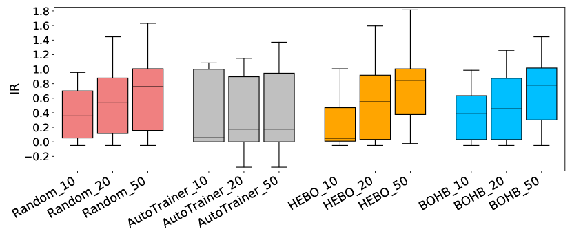
Figure 1: IR values from all faults in the benchmark, broken down by the combinations of repair technique and budget, shown as [technique]_[budget]. Note that some IR values are higher than 1.0, meaning that the corresponding patches are better than the ground truth patches.

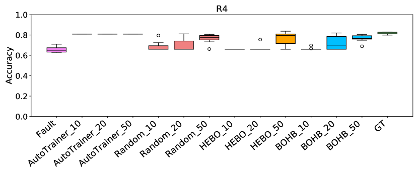
(a) Artificial fault R4

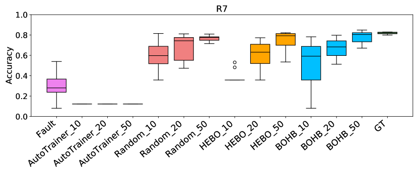
(b) Artificial fault R7

Figure 2: Example boxplots of the results from two artificial faults, showing the accuracy of the generated patches. The $x$-axis represents combinations of repair techniques and budgets, shown as [technique]_[budget].

The boxplot of each fault provides a closer look at how differently each technique performs depending on the type of fault. For example, Figure 2 presents the accuracy boxplots for two artificial faults. As shown in Figure 2(a), AutoTrainer easily and consistently fixes this fault, even with a small budget. While AutoTrainer’s coverage of different fault types is not that high, being generally lower than that of HPO techniques (see Tables I & II), when a fault type is in the scope of AutoTrainer, it can be effective, especially on simpler faults, such as mutants generated by DeepCrime, which by construction, can be fixed with a single repair operation. Faults M2, R4, and R5 in Table III are cases in which AutoTrainer finds good patches more easily than others. However, as shown in Figure 2(b), if there is no specific repair operator for the fault, AutoTrainer cannot find a good patch. In contrast, since HPO techniques are designed to apply multiple repair operators at once, they effectively search a wider space of patches and, thus, are more likely to find better patches for more complicated cases. While the overall trend is that the fixes produced by Random are better than AutoTrainer and are comparable with fixes by HPO techniques, this is not always the case. Also, the efficacy of a repair technique depends on the type of faults; there is no single best repair technique.

Answer to RQ1: In general, random baseline produces comparable or better patches than other repair techniques, but the effectiveness of tools varies depending on the fault, which justifies the need for future work to find more efficient ways of exploring the hyperparameter space.

V-B Stability (RQ2)

Table III shows the standard deviations ($\sigma$), which quantify the stability of the patches found by each tool across ten runs (i.e., $\sigma$ quantifies the performance variability of the best patched model across multiple executions of each tool). Below, we comment on the standard deviation of each tool, considering only the cases showing statistical significance of the model performance improvement.

AutoTrainer has the smallest average standard deviation of 0.006, followed by HEBO with 0.060, Random with 0.085, and BOHB with 0.094. AutoTrainer is shown to be the most stable technique: this is because, in principle, the number of repair operators being applied is relatively small compared to the others (see their coverages in Tables I & II and complexities in Section V-D for details), allowing it to generate consistent patches across executions, despite the randomness occurring in multiple runs. In contrast, HPO techniques, as well as Random, tend to produce more diverse and different patches, which implies that their patches are less stable in terms of patched model performance. This calls for future work to improve the stability of the repair techniques for DL models, especially when the patches are complex in terms of the number of changed hyperparameters and applied repair operators.

Answer to RQ2: AutoTrainer produces similar patches across several runs since it operates by applying operators selected from a relatively small set, while HPO techniques and Random produce varied patches, hence, they are more prone to instability.

V-C Costs (RQ3)

Automated program repair for traditional software usually requires a significant amount of time and computational resources, as it needs to search a large space of patches while running the tests for each candidate patch. Techniques such as Random and HPO also have similar issues because each patch requires training and validating its model from scratch.

We investigate three different time limits, 10, 20, and 50, under the assumption that developers may have different time constraints when repairing a faulty DL model. Due to lack of space, we report only a time limit of 20 in Table III (full results are available in online supplementary material). As expected, all techniques produce more patches showing the statistical significance of the improvements when larger budgets are allowed. For instance, Random finds patches showing statistical significance in 14 cases with a 10 time budget, which becomes 17 cases with a 20 time budget and 23 cases with a 50 time budget. This trend is consistent even considering IR, as shown in Figure 1: larger time budget results in larger IR as well as a smaller standard deviation. AutoTrainer does not take advantage so much of a larger time budget, compared to the other techniques, due to its limited search space. HEBO can be a good alternative to Random when the budget is large such as 50: it shows slightly better performance than Random with a smaller standard deviation.

Overall, given larger budgets, our results support the use of HPO techniques, such as HEBO, which are preferable to AutoTrainer because of the narrower scope of the latter.

Answer to RQ3: For all DL repair techniques, using a larger time budget results in more stable and better patches. The results also show that AutoTrainer does not benefit from larger budgets, while HPO techniques can benefit from them.

V-D Patch Complexity (RQ4)

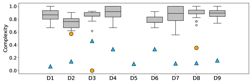
(a) Real faults

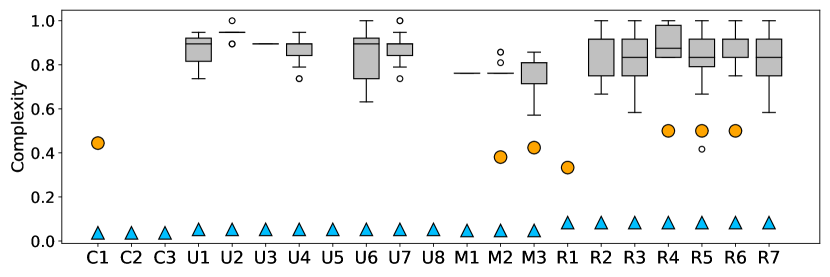
(b) Artificial faults

Figure 3: Complexities of statistically significant patches. Boxplots represent HPO and Random’s patchesfn:complexity; triangles the ground truth’s one and circles the AutoTrainer’s one.

Figure 3 presents the boxplots of the complexity of the statistically significant patches generated by HPO techniques and Random with time budget 20. The blue triangles and orange circles show the complexity of the ground truth patches and AutoTrainer’s patches, respectively. Overall, the complexity of the generated patches of HPO and Random is much higher than the complexity of the ground truth patches. This means that the generated patches manipulate many different hyperparameters (around 80% to 90% of them) to achieve an improvement of the faulty model. In contrast, a ground truth patch makes fewer changes, despite achieving similar or higher evaluation metric values. The main reason for this difference is that both Random and HPO explore the hyperparameter space at large in search for configurations that improve the model’s accuracy. Random is completely unconstrained in its exploration: thus, it is expected that it can generate solutions that are far from the initial faulty model. HPO, on the other hand, balances exploitation (i.e., local improvements of the best model found so far, which at the beginning is the initial faulty model) and exploration (i.e., it samples new diversified points in the hyperparameter space to avoid getting stuck in a local minimum). Consequently, the results suggest that, in our subjects, the exploration component is dominant, and improvements are obtained only when HPO techniques moved away from the initial model.

In general, the patches generated by AutoTrainer have lower complexity than Random and HPO. This is consistent with its design principle: it can handle a narrow set of repair actions, targeting specific fault types, which makes the tool either effective and capable of improving the initial solution with a small number of changes or completely ineffective.

Despite the high complexity, the observed AJ values suggest that the generated patches do contain the same ingredients as the ground truth patches, i.e., they include similar repair operators. For real faults, the AJ values for HPO and Random have a mean of 0.97 and a standard deviation of 0.11; for artificial faults, 0.90 and 0.29, respectively. The AJ values for AutoTrainer, however, reflect its narrower repair scope, with a mean and standard deviation of 0.26 and 0.19 for real faults, and 0.61 and 0.49 for artificial faults, respectively. Considering this, in conjunction with the high complexity values, we suggest that the generated patches may be bloated, i.e., they contain redundant changes when compared to the ground truth.

Answer to RQ4: The complexity of the patches generated by HPO techniques and Random are high compared to the ones of the ground truth and of AutoTrainer, which demands better Bayesian optimisation algorithms that can take advantage of the initial, faulty model.

VI Discussion

The analysis of the existing benchmarks of real faults currently used in the literature has revealed that the majority of real faults collected so far are rather simplistic. In many cases, the models represent toy examples for naive tasks and data used to train and test the models are either randomly generated or too small. On the other hand, the artificial faults produced by DeepCrime cover a larger variety of fault types and affect more diverse and complex models.

Indeed, in our empirical evaluation, artificial faults were more challenging to repair than the real ones. The evaluated approaches are either unable to reach the performance of an un-mutated model or show a high standard deviation across repair repetitions. A common pattern we observed in the results is that on large models such as CIFAR10 model, all techniques could not generate any successful fixes (see C2 and C3 in Table III). Since the number of hyperparameters of the CIFAR10 model is 27, which is twice bigger than that of the Reuters model, the search space is relatively large, so it becomes more difficult to find patches. While developing more advanced search techniques to deal with large models is a promising direction for future work, the other option would be combining Fault Localisation (FL) [24, 25] and repair techniques. FL techniques can narrow down the search space and pinpoint the locations of a fault (i.e., faulty hyperparameters), which can be used as a starting point for the repair techniques. See Section VIII-B for more details on FL techniques.

Future work could include various repair operations. We used nine frequent fault types, but this selection is insufficient to cover all faults in real world. In particular, the existing repair operations and techniques do not cover faults related to the quality and pre-processing of training and test data.

Compared to traditional Automated Program Repair (APR) techniques for source code, one critical step that is missing in model architecture repair is patch minimisation. Although, our analysis shows that smaller patches do exist and such patches are useful for developers, minimization might be difficult due to the stochastic nature of model repair. Existing model slicing [61] and pruning [62] techniques tend to apply directly to the trained models and not to the source code that defines the model architecture. Patch minimisation for model architecture faults remains an unexplored area.

Lastly, our results open up a new direction of research that targets the space of higher-order patches by smaller and more local changes of the initial, faulty model. In fact, HPO techniques are designed to start from scratch far from the initial hyperparameters. Intensification of the search around the initial faulty model seems a promising research direction.

VII Threats to Validity

One of the threats to internal validity is the selection of the HPO algorithms. We carefully studied state of the art in HPO algorithms and chose novel and best-performing approaches as well as generally accepted baseline. To avoid incorrect implementations of those algorithms, we used widely used libraries and frameworks. The main threat to external validity is the construction of the benchmark used for the comparison of the approaches. To mitigate any risks, we included both artificial faults that cover a variety of subjects and a dataset of real faults used in the previous literature. All the faults included in our benchmark were obtained through a methodologically sound selection procedure. Threats to construct validity lie in a correct measurement of the performance of the repair tools. All evaluation metrics used in the benchmark are standard and widely used in the ML literature. For what concerns conclusion validity, we measured effect size using our custom metric IR and statistical significance using Wilcoxon’s test.

VIII Related Work

VIII-A Model-level Repair

To the best of our knowledge, no automatic source-level repair tool currently exists that aims to fix the performance of a given faulty DL model by applying patches to the source code that defines the model’s architecture and hyperparameters. As discussed in Section II, the closest approaches come from machine learning, in particular, those solving the HPO problem, and from software engineering, AutoTrainer, a tool that continues to train an already trained model using patched hyperparameters. The goal of our empirical study was to compare these two families of approaches when adapted to solve the model architecture repair problem. No previous empirical study attempted to conduct any similar comparison.

On the other hand, post-training, model-level repair of DNN networks, i.e., repair through the modification of the weights of an already trained model, is gaining increasing popularity. CARE [63] identifies and modifies weights of neurons that contribute to detected model misbehaviors until the defects are eliminated. Arachne [64] operates similarly to CARE while ensuring the non-disturbance of the correct behaviour of a model under repair. GenMuNN [65] ranks the weights based on the effect on predictions. Using the computed ranks, it generates mutants and evaluates and evolves them using a genetic algorithm. NeuRecover [66] keeps track of the training history to find the weights that have changed significantly over time. Such weights become a subject for repair if they are not beneficial for the prediction of the successfully learnt inputs but have become detrimental for the inputs that were correctly classified in the earlier stages of the training. Similarly to NeuRecover, I-Repair [67] focuses on modifying localised weights to influence the predictions for a certain set of misbehaving inputs, whereas minimising the effect on the data that was already correctly classified. NNrepair [68] adopts fault localisation to pinpoint suspicious weights and treats them by using constraint solving, resulting in minor modifications of weights.

PRDNN [69] took a slightly different path by focusing on the smallest achievable single-layer repair. If provided with a limited set of problematic inputs and a model, this algorithm returns a repaired DNN that produces correct output for these and similar inputs and retains the model’s behaviour for other, dissimilar kinds of data. Apricot [21], however, uses a DL model trained on a reduced subset of inputs and then uses the weights of the reduced model to adjust the weights of the full model to fix its misbehaviour on the inputs from the reduced dataset. In our work, we are interested in the approaches that recommend changes to the model’s source code rather than patching the weights of the model.

VIII-B Fault Localisation

Fault localisation in DNNs is a rapidly evolving area of DL testing [70, 25, 24, 71, 72]. Most of the proposed approaches focus on analysing the run-time behaviour during the model training. According to the collected information and some predefined rules, these approaches decide whether they can spot any abnormalities and report them [70, 25, 72].

During the training of a model, both DeepDiagnosis [25] and DeepLocalize [70] insert a callback that collects various performance indicators such as loss function values, weights, gradients and activations. Both tools then compare the analysed values with a list of pre-defined failure symptoms. UMLAUT [72] combines heuristic static checks of the model structure and its parameters with dynamic monitoring of the training and the model behaviour. It complements the results of the checks with the analysis of the error messages, providing best practices and suggestions on how to deal with the faults.

Unlike previously discussed methods, Neuralint [71] is a model-based approach that employs meta-modelling and graph transformations for fault detection. Given a model under test, it constructs a meta-model consisting of the base skeleton and some fundamental properties. This model is then checked against a set of 23 rules embodied in graph transformations, each representing a fault or a design issue. DeepFD [24] employs mutation testing to construct a database of mutants and their original models to train a fault type ML classifier. From the mutants, it extracts a number of runtime features and use several combinations of them to localise the faults.

Although all of these approaches are potentially useful for the task of automated repair of DNNs, they just provide suggestions without any detailed instructions on how to change the faulty model. Hence, they could not be included in our empirical comparison of DL repair tools.

IX Conclusion

In this work, we evaluate techniques proposed in the ML and SE research communities that are applicable to the problem of repair of DNN architecture faults. In particular, we compare the state-of-the-art hyperparameter tuning algorithms HEBO [27] and BOHB [28], which are based on Bayesian optimisation, and the recent DNN repair tool called AutoTrainer [26], while using random search as a baseline. To allow a thorough assessment, we apply these techniques to a carefully collected benchmark of real and artificial faults. The obtained results indicate that all of the evaluated techniques are able to enhance the performance of fault models in some cases but are often not as effective as the ground truth fixes. Moreover, the generated patches tend to have a higher complexity than that of the ground truth. According to our observations, for simpler models, more advanced approaches do not happen to outperform random search, whilst random search and HPO algorithms clearly surpass AutoTrainer. For more complex models, all considered approaches fail to perform well. Thus, there is ample space for improvement in the area of DNN model architecture repair. Furthermore, our findings reveal a number of promising future research directions: a synergy with DNN fault localisation techniques, the need for more sophisticated repair operators and algorithms, and the need for patch minimisation.

References

- [1] G. Hinton, L. Deng, D. Yu, G. E. Dahl, A. Mohamed, N. Jaitly, A. Senior, V. Vanhoucke, P. Nguyen, T. N. Sainath, and B. Kingsbury, “Deep neural networks for acoustic modeling in speech recognition: The shared views of four research groups,” IEEE Signal Processing Magazine, vol. 29, no. 6, pp. 82–97, Nov 2012.
- [2] A. Krizhevsky, I. Sutskever, and G. E. Hinton, “Imagenet classification with deep convolutional neural networks,” Commun. ACM, vol. 60, no. 6, pp. 84–90, May 2017. [Online]. Available: http://doi.acm.org/10.1145/3065386
- [3] X. Chen, H. Ma, J. Wan, B. Li, and T. Xia, “Multi-view 3d object detection network for autonomous driving,” in Proceedings of the IEEE Conference on Computer Vision and Pattern Recognition, 2017, pp. 1907–1915.
- [4] C. Chen, A. Seff, A. Kornhauser, and J. Xiao, “Deepdriving: Learning affordance for direct perception in autonomous driving,” in Proceedings of the IEEE International Conference on Computer Vision, 2015, pp. 2722–2730.
- [5] I. Sutskever, O. Vinyals, and Q. V. Le, “Sequence to sequence learning with neural networks,” in Proceedings of the 27th International Conference on Neural Information Processing Systems, ser. NIPS’14. Cambridge, MA, USA: MIT Press, 2014, pp. 3104–3112.
- [6] S. Jean, K. Cho, R. Memisevic, and Y. Bengio, “On using very large target vocabulary for neural machine translation,” in Proceedings of the 53rd Annual Meeting of the Association for Computational Linguistics and the 7th International Joint Conference on Natural Language Processing (Volume 1: Long Papers). Beijing, China: Association for Computational Linguistics, Jul. 2015, pp. 1–10. [Online]. Available: https://www.aclweb.org/anthology/P15-1001
- [7] B. J. Erickson, P. Korfiatis, Z. Akkus, and T. L. Kline, “Machine learning for medical imaging,” Radiographics, vol. 37, no. 2, p. 505, 2017.
- [8] G. Varoquaux and V. Cheplygina, “Machine learning for medical imaging: methodological failures and recommendations for the future,” NPJ digital medicine, vol. 5, no. 1, pp. 1–8, 2022.
- [9] D. Parekh, N. Poddar, A. Rajpurkar, M. Chahal, N. Kumar, G. P. Joshi, and W. Cho, “A review on autonomous vehicles: Progress, methods and challenges,” Electronics, vol. 11, no. 14, p. 2162, 2022.
- [10] V. Riccio and P. Tonella, “Model-based exploration of the frontier of behaviours for deep learning system testing,” in Proceedings of the 28th ACM Joint Meeting on European Software Engineering Conference and Symposium on the Foundations of Software Engineering, ser. ESEC/FSE 2020. New York, NY, USA: Association for Computing Machinery, 2020, pp. 876–888. [Online]. Available: https://doi.org/10.1145/3368089.3409730
- [11] J. Guo, Y. Jiang, Y. Zhao, Q. Chen, and J. Sun, “Dlfuzz: Differential fuzzing testing of deep learning systems,” in Proceedings of the 2018 26th ACM Joint Meeting on European Software Engineering Conference and Symposium on the Foundations of Software Engineering, ser. ESEC/FSE 2018. New York, NY, USA: Association for Computing Machinery, 2018, pp. 739–743. [Online]. Available: https://doi.org/10.1145/3236024.3264835
- [12] A. Gambi, M. Mueller, and G. Fraser, “Automatically testing self-driving cars with search-based procedural content generation,” in Proceedings of the 28th ACM SIGSOFT International Symposium on Software Testing and Analysis, ser. ISSTA 2019. New York, NY, USA: Association for Computing Machinery, 2019, pp. 318–328. [Online]. Available: https://doi.org/10.1145/3293882.3330566
- [13] I. Goodfellow, J. Shlens, and C. Szegedy, “Explaining and harnessing adversarial examples,” in International Conference on Learning Representations, 2015. [Online]. Available: http://arxiv.org/abs/1412.6572
- [14] A. Kurakin, I. J. Goodfellow, and S. Bengio, “Adversarial examples in the physical world,” CoRR, vol. abs/1607.02533, 2016. [Online]. Available: http://arxiv.org/abs/1607.02533
- [15] Y. Tian, K. Pei, S. Jana, and B. Ray, “Deeptest: Automated testing of deep-neural-network-driven autonomous cars,” in Proceedings of the 40th International Conference on Software Engineering, ser. ICSE ’18. New York, NY, USA: ACM, 2018, pp. 303–314. [Online]. Available: http://doi.acm.org/10.1145/3180155.3180220
- [16] K. Pei, Y. Cao, J. Yang, and S. Jana, “Deepxplore: Automated whitebox testing of deep learning systems,” in Proceedings of the 26th Symposium on Operating Systems Principles, ser. SOSP ’17. New York, NY, USA: ACM, 2017, pp. 1–18. [Online]. Available: http://doi.acm.org/10.1145/3132747.3132785
- [17] L. Ma, F. Juefei-Xu, F. Zhang, J. Sun, M. Xue, B. Li, C. Chen, T. Su, L. Li, Y. Liu, J. Zhao, and Y. Wang, “Deepgauge: Multi-granularity testing criteria for deep learning systems,” in Proceedings of the 33rd ACM/IEEE International Conference on Automated Software Engineering, ser. ASE 2018. New York, NY, USA: ACM, 2018, pp. 120–131. [Online]. Available: http://doi.acm.org/10.1145/3238147.3238202
- [18] J. Kim, R. Feldt, and S. Yoo, “Guiding deep learning system testing using surprise adequacy,” in Proceedings of the 41th International Conference on Software Engineering, ser. ICSE 2019. IEEE Press, 2019, pp. 1039–1049.
- [19] X. Huang, M. Kwiatkowska, S. Wang, and M. Wu, “Safety verification of deep neural networks,” in Computer Aided Verification, R. Majumdar and V. Kunčak, Eds. Cham: Springer International Publishing, 2017, pp. 3–29.
- [20] X. Gao, R. K. Saha, M. R. Prasad, and A. Roychoudhury, “Fuzz testing based data augmentation to improve robustness of deep neural networks,” in Proceedings of the ACM/IEEE 42nd International Conference on Software Engineering, ser. ICSE ’20. New York, NY, USA: Association for Computing Machinery, 2020, pp. 1147–1158. [Online]. Available: https://doi.org/10.1145/3377811.3380415
- [21] H. Zhang and W. K. Chan, “Apricot: A weight-adaptation approach to fixing deep learning models,” in 2019 34th IEEE/ACM International Conference on Automated Software Engineering (ASE), 2019, pp. 376–387.
- [22] S. Ma, Y. Liu, W.-C. Lee, X. Zhang, and A. Grama, “Mode: Automated neural network model debugging via state differential analysis and input selection,” in Proceedings of the 2018 26th ACM Joint Meeting on European Software Engineering Conference and Symposium on the Foundations of Software Engineering, ser. ESEC/FSE 2018. New York, NY, USA: ACM, 2018, pp. 175–186. [Online]. Available: http://doi.acm.org/10.1145/3236024.3236082
- [23] N. Humbatova, G. Jahangirova, G. Bavota, V. Riccio, A. Stocco, and P. Tonella, “Taxonomy of real faults in deep learning systems,” in The proceedings of the 42nd IEEE/ACM International Conference on Software Engineering, ser. ICSE 2020, 2020, pp. 1110–1121.
- [24] J. Cao, M. Li, X. Chen, M. Wen, Y. Tian, B. Wu, and S.-C. Cheung, “DeepFD: Automated fault diagnosis and localization for deep learning programs,” in Proceedings of the 44th International Conference on Software Engineering, ser. ICSE 2022. ACM, 2022.
- [25] M. Wardat, B. D. Cruz, W. Le, and H. Rajan, “DeepDiagnosis: automatically diagnosing faults and recommending actionable fixes in deep learning programs,” in Proceedings of the 44th International Conference on Software Engineering, 2022, pp. 561–572.
- [26] X. Zhang, J. Zhai, S. Ma, and C. Shen, “Autotrainer: An automatic dnn training problem detection and repair system,” in 2021 IEEE/ACM 43rd International Conference on Software Engineering (ICSE). IEEE, 2021, pp. 359–371.
- [27] A. I. Cowen-Rivers, W. Lyu, R. Tutunov, Z. Wang, A. Grosnit, R. R. Griffiths, A. M. Maraval, H. Jianye, J. Wang, J. Peters et al., “Hebo: Pushing the limits of sample-efficient hyper-parameter optimisation,” Journal of Artificial Intelligence Research, vol. 74, pp. 1269–1349, 2022.
- [28] S. Falkner, A. Klein, and F. Hutter, “Bohb: Robust and efficient hyperparameter optimization at scale,” in International Conference on Machine Learning. PMLR, 2018, pp. 1437–1446.
- [29] H. Jin, Q. Song, and X. Hu, “Auto-keras: An efficient neural architecture search system,” in Proceedings of the 25th ACM SIGKDD International Conference on Knowledge Discovery & Data Mining, KDD, 2019, pp. 1946–1956.
- [30] N. Humbatova, G. Jahangirova, and P. Tonella, “DeepCrime: Mutation testing of deep learning systems based on real faults,” in Proceedings of the 30th ACM SIGSOFT International Symposium on Software Testing and Analysis, ser. ISSTA 2021. New York, NY, USA: Association for Computing Machinery, 2021, p. 67–78. [Online]. Available: https://doi.org/10.1145/3460319.3464825
- [31] Y. LeCun, C. Cortes, and C. Burges, “Mnist handwritten digit database,” AT&T Labs [Online]. Available: http://yann. lecun. com/exdb/mnist, vol. 2, 2010.
- [32] A. Krizhevsky, “Learning multiple layers of features from tiny images,” University of Toronto, Tech. Rep., 2009.
- [33] “Keras Reuters Dataset,” 2021, available at https://keras.io/api/datasets/reuters/.
- [34] E. Wood, T. Baltrušaitis, L.-P. Morency, P. Robinson, and A. Bulling, “Learning an appearance-based gaze estimator from one million synthesised images,” ser. ETRA ’16. New York, NY, USA: Association for Computing Machinery, 2016, p. 131–138. [Online]. Available: https://doi.org/10.1145/2857491.2857492
- [35] M. Claesen and B. De Moor, “Hyperparameter search in machine learning,” arXiv preprint arXiv:1502.02127, 2015.
- [36] M. Feurer and F. Hutter, “Hyperparameter optimization,” in Automated machine learning. Springer, Cham, 2019, pp. 3–33.
- [37] A. Zela, A. Klein, S. Falkner, and F. Hutter, “Towards automated deep learning: Efficient joint neural architecture and hyperparameter search,” arXiv preprint arXiv:1807.06906, 2018.
- [38] D. C. Montgomery, Design and analysis of experiments. John wiley & sons, 2017.
- [39] J. Bergstra and Y. Bengio, “Random search for hyper-parameter optimization.” Journal of machine learning research, vol. 13, no. 2, 2012.
- [40] E. Brochu, V. M. Cora, and N. De Freitas, “A tutorial on bayesian optimization of expensive cost functions, with application to active user modeling and hierarchical reinforcement learning,” arXiv preprint arXiv:1012.2599, 2010.
- [41] D. R. Jones, “A taxonomy of global optimization methods based on response surfaces,” Journal of global optimization, vol. 21, no. 4, pp. 345–383, 2001.
- [42] M. J. Sasena, Flexibility and efficiency enhancements for constrained global design optimization with kriging approximations. University of Michigan, 2002.
- [43] J. Snoek, H. Larochelle, and R. P. Adams, “Practical bayesian optimization of machine learning algorithms,” Advances in neural information processing systems, vol. 25, 2012.
- [44] J. Snoek, O. Rippel, K. Swersky, R. Kiros, N. Satish, N. Sundaram, M. Patwary, M. Prabhat, and R. Adams, “Scalable bayesian optimization using deep neural networks,” in International conference on machine learning. PMLR, 2015, pp. 2171–2180.
- [45] G. Melis, C. Dyer, and P. Blunsom, “On the state of the art of evaluation in neural language models,” arXiv preprint arXiv:1707.05589, 2017.
- [46] G. E. Dahl, T. N. Sainath, and G. E. Hinton, “Improving deep neural networks for lvcsr using rectified linear units and dropout,” in 2013 IEEE international conference on acoustics, speech and signal processing. IEEE, 2013, pp. 8609–8613.
- [47] K. Jamieson and A. Talwalkar, “Non-stochastic best arm identification and hyperparameter optimization,” in Artificial intelligence and statistics. PMLR, 2016, pp. 240–248.
- [48] L. Li, K. Jamieson, G. DeSalvo, A. Rostamizadeh, and A. Talwalkar, “Hyperband: A novel bandit-based approach to hyperparameter optimization,” The Journal of Machine Learning Research, vol. 18, no. 1, pp. 6765–6816, 2017.
- [49] Y. Jia and M. Harman, “An analysis and survey of the development of mutation testing,” IEEE transactions on software engineering, vol. 37, no. 5, pp. 649–678, 2011.
- [50] G. Jahangirova and P. Tonella, “An empirical evaluation of mutation operators for deep learning systems,” in 2020 IEEE 13th International Conference on Software Testing, Validation and Verification (ICST). IEEE, 2020, pp. 74–84.
- [51] W. Shen, J. Wan, and Z. Chen, “Munn: Mutation analysis of neural networks,” in 2018 IEEE International Conference on Software Quality, Reliability and Security Companion (QRS-C). IEEE, 2018, pp. 108–115.
- [52] L. Ma, F. Zhang, J. Sun, M. Xue, B. Li, F. Juefei-Xu, C. Xie, L. Li, Y. Liu, J. Zhao et al., “Deepmutation: Mutation testing of deep learning systems,” in 2018 IEEE 29th International Symposium on Software Reliability Engineering (ISSRE). IEEE, 2018, pp. 100–111.
- [53] Q. Hu, L. Ma, X. Xie, B. Yu, Y. Liu, and J. Zhao, “Deepmutation++: A mutation testing framework for deep learning systems,” in 2019 34th IEEE/ACM International Conference on Automated Software Engineering (ASE), 2019, pp. 1158–1161.
- [54] M. J. Islam, G. Nguyen, R. Pan, and H. Rajan, “A comprehensive study on deep learning bug characteristics,” in Proceedings of the 2019 27th ACM Joint Meeting on European Software Engineering Conference and Symposium on the Foundations of Software Engineering, 2019, pp. 510–520.
- [55] Y. Zhang, Y. Chen, S.-C. Cheung, Y. Xiong, and L. Zhang, “An empirical study on tensorflow program bugs,” in Proceedings of the 27th ACM SIGSOFT International Symposium on Software Testing and Analysis, 2018, pp. 129–140.
- [56] “DeepCrime Replication Package,” 2020. [Online]. Available: https://zenodo.org/record/4772465
- [57] Y. LeCun, “The MNIST Database of Handwritten Digits,” 1998, available at http://yann.lecun.com/exdb/mnist/.
- [58] “The Keras CIFAR10 Dataset of Colour Images,” 2000, available at https://keras.io/api/datasets/cifar10/.
- [59] D. P. Kingma and J. Ba, “Adam: A method for stochastic optimization,” arXiv preprint arXiv:1412.6980, 2014.
- [60] R. Liaw, E. Liang, R. Nishihara, P. Moritz, J. E. Gonzalez, and I. Stoica, “Tune: A research platform for distributed model selection and training,” arXiv preprint arXiv:1807.05118, 2018.
- [61] Z. Zhang, Y. Li, Y. Guo, X. Chen, and Y. Liu, “Dynamic slicing for deep neural networks,” in Proceedings of the 28th ACM Joint Meeting on European Software Engineering Conference and Symposium on the Foundations of Software Engineering, ser. ESEC/FSE 2020. New York, NY, USA: Association for Computing Machinery, 2020, pp. 838–850.
- [62] N. Liu, X. Ma, Z. Xu, Y. Wang, J. Tang, and J. Ye, “Autocompress: An automatic dnn structured pruning framework for ultra-high compression rates,” Proceedings of the AAAI Conference on Artificial Intelligence, vol. 34, no. 04, pp. 4876–4883, Apr. 2020.
- [63] B. Sun, J. Sun, L. H. Pham, and J. Shi, “Causality-based neural network repair,” in Proceedings of the 44th International Conference on Software Engineering, 2022, pp. 338–349.
- [64] J. Sohn, S. Kang, and S. Yoo, “Arachne: Search based repair of deep neural networks,” ACM Transactions on Software Engineering Methodology, vol. to appear, 2022.
- [65] H. Wu, Z. Li, Z. Cui, and J. Liu, “Genmunn: A mutation-based approach to repair deep neural network models,” International Journal of Modeling, Simulation, and Scientific Computing, p. 2341008, 2022.
- [66] S. Tokui, S. Tokumoto, A. Yoshii, F. Ishikawa, T. Nakagawa, K. Munakata, and S. Kikuchi, “Neurecover: Regression-controlled repair of deep neural networks with training history,” arXiv preprint arXiv:2203.00191, 2022.
- [67] P. Henriksen, F. Leofante, and A. Lomuscio, “Repairing misclassifications in neural networks using limited data,” in Proceedings of the 37th ACM/SIGAPP Symposium on Applied Computing, 2022, pp. 1031–1038.
- [68] M. Usman, D. Gopinath, Y. Sun, Y. Noller, and C. S. Păsăreanu, “Nn repair: Constraint-based repair of neural network classifiers,” in International Conference on Computer Aided Verification. Springer, 2021, pp. 3–25.
- [69] M. Sotoudeh and A. V. Thakur, “Provable repair of deep neural networks,” in Proceedings of the 42nd ACM SIGPLAN International Conference on Programming Language Design and Implementation, 2021, pp. 588–603.
- [70] M. Wardat, W. Le, and H. Rajan, “Deeplocalize: Fault localization for deep neural networks,” in 2021 IEEE/ACM 43rd International Conference on Software Engineering (ICSE). IEEE, 2021, pp. 251–262.
- [71] A. Nikanjam, H. B. Braiek, M. M. Morovati, and F. Khomh, “Automatic fault detection for deep learning programs using graph transformations,” ACM Transactions on Software Engineering and Methodology (TOSEM), vol. 31, no. 1, pp. 1–27, 2021.
- [72] E. Schoop, F. Huang, and B. Hartmann, “Umlaut: Debugging deep learning programs using program structure and model behavior,” in Proceedings of the 2021 CHI Conference on Human Factors in Computing Systems, 2021, pp. 1–16.