Exponential tail bounds and Large Deviation Principle for Heavy-Tailed U-Statistics

Abstract

We study deviation of U-statistics when samples have heavy-tailed distribution so the kernel of the U-statistic does not have bounded exponential moments at any positive point. We obtain an exponential upper bound for the tail of the U-statistics which clearly denotes two regions of tail decay, the first is a Gaussian decay and the second behaves like the tail of the kernel. For several common U-statistics, we also show the upper bound has the right rate of decay as well as sharp constants by obtaining rough logarithmic limits which in turn can be used to develop LDP for U-statistics. In spite of usual LDP results in the literature, processes we consider in this work have LDP speed slower than their sample size $n$.

1 Introduction

Suppose $X_{1},X_{2},\ldots,X_{n}\overset{iid}{\sim}\mu$ where $\mu$ is a probability measure supported on $\mathbb{R}$. We consider the following U-statistic of order $m$ with a kernel function $h(\cdot)\mathrel{\mathop{\mathchar 58\relax}}\mathbb{R}^{m}\to\mathbb{R}$ which is symmetric about its arguments:

$$U_{n}\triangleq\frac{1}{{n\choose m}}\sum_{1\leq i_{1}<\ldots<i_{m}\leq n}h(X_{i_{1}},\ldots,X_{i_{m}}).$$

We study the decay of $\mathbb{P}\left({\mathinner{\!\left\lvert U_{n}-\mathbb{E}\mathinner{\left[U_{n}\right]}\right\rvert}>t}\right)$ as a function of $t,n$, and $m$, in a setup which is rarely addressed in the literature and is characterized by a couple of key assumptions: heavy-tailed distribution for $h(X_{1},...,X_{m})$, and large values for $t$. We explain the role of each assumption in more details below.

When $h(X_{1},...,X_{m})\triangleq h$ has a heavy-tailed distribution, its Moment Generating Function (MGF) is not bounded at any positive point. This breaks many concentration results and violates Cramer’s condition which is required for common results that determine large deviation behavior. While deviation of U-statistics has been studied extensively in the light-tailed regime [1, 9, 8, 15, 16, 23, 22], the same for heavy-tailed U-statistics is relatively under-explored. In this paper, we aim to focus on the heavy-tailed regime.

Moreover, when kernel $h$ is assumed to have a heavy tail, for fixed values of $n$ and $m$, $\mathbb{P}\left({\mathinner{\!\left\lvert U_{n}-\mathbb{E}\mathinner{\left[U_{n}\right]}\right\rvert}>t}\right)$ has two different behaviors: 1) for small values of $t$ it decays like a Gaussian tail, and 2) for $t$ larger than the zone of normal convergence, i.e. large deviation zone, it has a decay slower than normal distribution. In spite of the first region which has been studied in the literature largely, see [16, 15] and the references therein, there are little documented information about the tail behavior in the second region. Several setups have been developed to study the behavior of the tail. We mention some of them below to discuss the setup that results of the current paper belong to.

1. Finite sample concentration inequalities that give upper bounds for $\mathbb{P}\left({\mathinner{\!\left\lvert U_{n}-\mathbb{E}\mathinner{\left[U_{n}\right]}\right\rvert}>t}\right)$ for all values of n.

2. Asymptotic distribution studies that find suitable scaling $a_{n}$ and limiting distribution $D$ for which $a_{n}\mathinner{\!\left\lvert U_{n}-\mathbb{E}\mathinner{\left[U_{n}\right]}\right\rvert}\xrightarrow{d}D$. $a_{n}=c\sqrt{n}$, and $D=\mathcal{N}(0,1)$ is the well-known CLT that holds for non-degenerate U-statistics.

3. Berry–Esseen type inequalities that seek for uniform upper bound $\mathinner{\!\left\lvert\mathbb{P}\left({a_{n}\mathinner{\!\left\lvert U_{n}-\mathbb{E}\mathinner{\left[U_{n}\right]}\right\rvert}>t}\right)-\phi(t)\right\rvert}$ for all $t\in\mathcal{C}$, where $\mathcal{C}\subseteq\mathbb{R}$.

4. Large deviation studies that look for convergence speed $b_{n}$ and rate function $f(t)$ for which we have $\lim\limits_{n\to\infty}\frac{-\log\mathbb{P}\left({\mathinner{\!\left\lvert U_{n}-\mathbb{E}\mathinner{\left[U_{n}\right]}\right\rvert}>t}\right)}{b_{n}}=f(t),\;f(t)>0$ for large $t$.

In this work, we try to shed some light on the undocumented facts about the deviation of U-statistics in setups 1 and 4 listed above, the concentration inequality, and the large deviation setups. In particular, we develop a general concentration inequality that holds for all U-statistics with finite second moments. Moreover, we characterize a class of kernels for which that concentration inequality is sharp enough to yield the large deviation limit. The byproduct of such sharpness analysis is obtaining exact convergence speed $b_{n}$ and a closed form for the rate function in terms of the tail of the kernel $h$. For heavy-tailed kernels, which are considered in this work, we usually obtain $b_{n}\ll n$, e.g $b_{n}=n^{\alpha},\;\alpha<1$. This distinguishes our results from several previous works that tried to determine tail behavior in the asymptotic Gaussian regime, i.e. $b_{n}=n$.

1.1 Related works

Large deviations of U-statistics have been studied in several previous works under a variety of assumptions. Hoeffiding [12] formally introduced U-statistics and showed with the right scaling they converge to a Normal distribution. Follow up studies offered bounds for the deviation of U-statistics from their Gaussian limits (see [16, 15] and the references therein).

Giné et al. [11] offers upper bound for moments of U-statistics. There is a relatively straightforward connection between moment inequalities and exponential bounds for the tail (see [21]). Utilizing such connection, [11] obtains exponential tail bounds. However, these bounds do not show Gaussian decay when the deviation amount $t$ is within the Gaussian zone. Therefore, the authors also offer improvements for their inequalities in the case of completely degenerate kernels of order $m=2$.

Recently, Chakrabortty and Kuchibhotla [5] considered degenerate kernels of order 2 and samples from heavy-tailed subWeibull distributions and obtained exponential tail bounds for such U-statistics. However, the specific form they used for the U-statistics seems restrictive. They define

$$U_{n}=\sum\limits_{i\neq j}\phi(Y_{i})w_{i,j}(X_{i},X_{j})\psi(Y_{j}),$$

and impose uniform boundedness assumption on $w_{i,j}$. Hence, the kernel can be unbounded only through product function $\phi(Y_{i})\psi(Y_{j})$. It is not clear to us if results of [5] can recover exponential bounds for general non-degenerate kernels like ones named in Lemma 2.19 of the current work.

One property of U-statitics of order $m\geq 2$ that makes them more challenging than the case $m=1$, i.e. iid sums, is containing dependent terms in the sum. There are a couple of ways to handle such dependencies, decoupling and martingale inequalities. Each direction points to a path that is relatively different from another. Both directions have been explored to develop tail bounds for U-statistics.

de la Pena [7] provides a decoupling tool that helps one to get rid of dependencies of summands in the U-statistics. This tool has been utilized by several later works to obtain exponential concentration bounds, e.g. [17, 4, 5]. While the decoupling technique is proved very powerful in handling dependencies, there is an extra $8$ factor on the upper bound it offers which usually makes the exponential bound it provides off by a constant factor in its exponent.

Another approach to obtain exponential inequalities for U-statistics is to leverage inequalities for (sub/super) martingales such as those in [10]. Houdré and Reynaud-Bouret [13] and some of their references pursue this direction. Using de la Pena [7] decoupling and Talagrand [20] inequality is common in such approach. Nevertheless, in this approach, the statements get algebraically complicated soon and several constants given by $\sup$ or expectation of partial sums get involved. As a result, many bounds obtained by martingale inequalities are restricted to order 2 or degenerate kernels. Moreover, constants are not usually sharp for the similar reason discussed in utilizing the decoupling technique above.

In addition to tail bounds, several works have been devoted to showing U-statistics satisfy Large Deviation Principal (LDP). It is common for works in this direction to assume the kernel has finite exponential moments, hence they exclude distributions we are focusing on in the current manuscript.

Dasgupta [6] tried to show large deviation behavior of U-statistics is determined by their conditional expectation given one summand. At the first glance this sounds a reasonable claim since the asymptotic normality of U-statistics is tightly related to such conditional expectations [12]. However, this claim has been disapproved later [3, 22].

Nikitin and Ponikarov [18] study large deviation of U-statistics with bounded non-degenerate kernels. It also claims no large deviation results have been known by the time the work was published. Arcones [1] developes a decomposition technique for the case of a 2-variables kernel with finite MGF that enables one to prove LDP. Nevertheless, extension of this technique to higher order kernels is not straightforward. Eichelsbacher and Löwe [9] consider both U-statistics and V-statistics, which includes terms with repeated samples in the sum, given by a kernel function with bounded MGF. In this case, they show satisfying LDP for U-statistics and the corresponding V-statistics is equivalent with the same rate function. Lemma 3.1 from [9], which allows one to bound MGF of a U-statistic, is one the most important tools we used in the current work. Eichelsbacher [8] provides sufficient conditions under which a U-statistic would satisfy an LDP under weak Cramer condition. It utilizes a representation of a bi-variable kernel as infinite sums of separable functions in order to reduce the problem of the large deviation for U-statistics to the one for sums of iid variables. Then, it applies contraction theorem to prove LDP for the U-statistics.

The current work focuses on heavy-tailed distributions which are mostly excluded from large deviation studies above. The exponential tail bound given in Section 2.1 includes all kernels with finite variances regardless of their order, boundedness, or degeneracy. The upper bound we offer is simple enough to reveal both Gaussian and heavy tail decay regions immediately. All parameters in the statement of the upper bound have known limits when $n\to\infty$. Moreover, we offer ready-to-use tools to handle them for fixed sample size $n$ in Section 2.1.1. In addition, to the best of our knowledge, the rough logarithmic limits, with speeds slower than $n$, obtained in Section 2.3 have not been documented in earlier works.

1.2 Some Applications

U-statistics appear in several statistical analyses including point estimation, such as population variance [12], hypothesis testing [19], and statistical mechanics [14]. As a self-averaging function, it is quite natural to ask how fast a U-statistic concentrates around its mean.

In particular, for the asymptotic analysis of hypothesis testing, the speed and the rate function for the large deviation of such statistics are important. For instance, obtaining the values of Bahadur efficiency and Bahadur exact slope requires having LDP for the test function [19]. Moreover, the large deviation principle and exponential concentrations for U-statistics play substantial roles in the study of macroscopic limits of interacting particle systems and in general statistical mechanics [17]. Our result enables one to extend such theories when samples are drawn from a heavy-tailed distribution.

2 Main results

The main result of this paper is two-fold. First, in Section 2.1 we develop a general upper bound for the tail probability of U-statistics whose kernels have bounded variances. Second, in Section 2.3, we show for several kernel functions this upper bound is tight enough to determine the large deviation behavior of the U-statistics. If a centered kernel $h\mathrel{\mathop{\mathchar 58\relax}}\mathbb{R}^{m}\to\mathbb{R}$ satisfies the criteria discussed in Section 2.3 and $U_{n}$ denotes the U-statistic corresponding to $h$ with $n$ samples, we show in Lemma 2.14 that $\mathbb{P}\left({U_{n}>t}\right)$ and $\mathbb{P}\left({h>\frac{n}{m}t}\right)$ have the same asymptotic behavior in logarithmic sense, i.e.

$$\lim_{n\to\infty}\frac{\log\mathbb{P}\left({U_{n}>t}\right)}{\log\mathbb{P}\left({h>\frac{n}{m}t}\right)}=1.$$

Therefore, both the convergence speed and the rate function for large deviation of $U_{n}$ are determined by the tail of kernel $h$.

In addition, the lower bound developed in Section 2.2 reveals the event that is responsible for large deviations of $U_{n}$. Indeed, one of the $X_{1},...,X_{n}$ gets large enough to make all the summands it is contributing to exceed $\frac{n}{m}t$. There will be ${n-1}\choose{m-1}$ such terms in the expansion of $U_{n}$.

2.1 Finite sample upper bound

Without loss of generality, we will operate under the assumption that the kernel is centered.

Assumption 1.

Suppose $h$ is centered, i.e.

$$\mathbb{E}h(X_{1},\ldots,X_{m})=0.$$

We need to define rate functions $I,J$ as below.

Definition 2.1.

Let $I,J\mathrel{\mathop{\mathchar 58\relax}}\mathbb{R}^{\geq 0}\to\mathbb{R}^{\geq 0}$ be two non-decreasing functions that upperbound right tails of $h$ and $\mathinner{\!\left\lvert X_{i}\right\rvert}$ exponentially. In other words:

$$\mathbb{P}\left({h(X_{1},...,X_{m})>t}\right)\leq\exp\left({-I(t)}\right),\quad\forall t\geq 0,$$ (2.1)

$$\mathbb{P}\left({\mathinner{\!\left\lvert X_{i}\right\rvert}>t}\right)\leq\exp\left({-J(t)}\right),\quad\forall t\geq 0.$$ (2.2)

Note that one can simply take $I(t)=-\log\mathbb{P}\left({h(X_{1},...,X_{m})>t}\right),\;J(t)=-\log\mathbb{P}\left({\mathinner{\!\left\lvert X_{i}\right\rvert}>t}\right)$. The whole point of Definition 2.1 is to allow one to work with possibly simpler upper bounds.

Below Lemma is a simpler modified version of Lemma 3.1 from [9].

Lemma 2.2.

Let $k\triangleq\lfloor\frac{n}{m}\rfloor$. Then, given any $L\geq 0$ and $\lambda\geq 0$, the following holds:

$$\mathbb{E}\left[\exp\left(\lambda\frac{1}{{n\choose m}}\sum_{1\leq i_{1}<\ldots<i_{m}\leq n}h_{L}(X_{i_{1}},\ldots,X_{i_{m}})\right)\right]\leq\mathbb{E}\mathinner{\left[\exp\left({\frac{\lambda}{k}h_{L}(X_{1},...,X_{m})}\right)\right]}^{k},$$

where $h_{L}(X_{i_{1}},\ldots,X_{i_{m}})\triangleq h(X_{i_{1}},\ldots,X_{i_{m}})\mathbf{1}(h(X_{i_{1}},\ldots,X_{i_{m}})\leq L)$.

Proof.

Define $B(X_{1},...,X_{n})=\frac{1}{k}(h_{L}(X_{1},...,X_{m})+h_{L}(X_{m+1},...,X_{2m})+...+h_{L}(X_{km-m+1},...,X_{km}))$, then we have

$$\frac{1}{{n\choose m}}\sum_{i_{1}<...<i_{m}}h_{L}(X_{i_{1}},...,X_{i_{m}})=\frac{1}{n!}\sum_{\sigma\in S_{n}}B(X_{\sigma(1)},...,X_{\sigma(n)}).$$

Since $h_{L}\leq L$ is bounded, its moment generating function is finite at any positive point, hence we obtain

$$\mathbb{E}\left[\exp\left(\lambda\frac{1}{{n\choose m}}\sum_{1\leq i_{1}<\ldots<i_{m}\leq n}h_{L}(X_{i_{1}},\ldots,X_{i_{m}})\right)\right] =\mathbb{E}\left[\exp\left(\frac{\lambda}{{n!}}\sum_{\sigma}B(X_{\sigma(1)},...,X_{\sigma(n)})\right)\right]$$

$$\overset{*}{\leq}\frac{1}{n!}\sum_{\sigma}\mathbb{E}\mathinner{\left[\exp\left({\lambda B(X_{\sigma(1)},...,X_{\sigma(n)})}\right)\right]}$$

$$=\mathbb{E}\mathinner{\left[\exp\left({\lambda B(X_{1},...,X_{n})}\right)\right]}$$

$$=\mathbb{E}\mathinner{\left[\exp\left({\frac{\lambda}{k}h_{L}(X_{1},...,X_{m})}\right)\right]}^{k}.$$

To obtain inequality marked by $*$, we used the fact $\exp\left({\frac{1}{n!}\sum\lambda B\circ\sigma}\right)\leq\frac{1}{n!}\sum\exp\left({B\circ\sigma}\right)$ by convexity of the exponential function.

$\square$

For the sake of simplicity we drop arguments of $h(X_{1},...,X_{m}),h_{L}(X_{1},...,X_{m})$ and only write $h,h_{L}$

Lemma 2.3 (Lemma 1 of [2]).

If $\mathbb{E}\mathinner{\left[h\right]}=0$, for any $\eta,L\geq 0$ we have

$$\mathbb{E}\mathinner{\left[\exp(\eta h_{L})\right]}\leq\exp\left(\frac{v(L,\eta)}{2}\eta^{2}\right),$$

where $v(L,\eta)\triangleq\mathbb{E}\mathinner{\left[h_{L}^{2}\mathbf{1}(h\leq 0)+h_{L}^{2}\exp(\eta h_{L})\mathbf{1}(h>0)\right]}$.

Theorem 2.4.

Under Assumption 1, for any $0<\beta\leq 1,\;t\geq 0$

$$\mathbb{P}\left({U_{n}>t}\right)\leq\exp\left({-\frac{kt^{2}}{2v(kt,\beta\frac{I(kt)}{kt})}}\right)+\exp\left({-\beta I(kt)\max(\frac{1}{2},c(t,\beta,k))}\right)+{n\choose m}\exp\left({-I(kt)}\right),$$ (2.3)

where $v(\cdot,\cdot)$ is the same as in Lemma 2.3, $c(t,\beta,k)\triangleq 1-\frac{\beta}{2t}\frac{I(kt)}{kt}v(kt,\beta\frac{I(kt)}{kt})$, and $k=\lfloor\frac{n}{m}\rfloor$.

Proof.

Let show the U-statistic with kernel $h$ by $U_{n}(h)$

$$\mathbb{P}\left({U_{n}(h)>t}\right) \leq\mathbb{P}\left({U_{n}(h_{L})>t}\right)+\mathbb{P}\left({\exists i_{1},...,i_{m},\quad h(X_{i_{1}},...,X_{i_{m}})>L}\right)$$

$$\leq\exp\left({-\lambda t}\right)\mathbb{E}\mathinner{\left[\exp\left({\lambda U_{n}(h_{L})}\right)\right]}+{n\choose m}\exp\left({-I(L)}\right)$$

$${\leq}\exp\left({-\lambda t}\right)\left(\mathbb{E}\mathinner{\left[\exp\left({\frac{\lambda}{k}h_{L}}\right)\right]}\right)^{k}+{n\choose m}\exp\left({-I(L)}\right)\hskip 85.35826pt$$ Lemma 2.2

$$\leq\exp\left({-\lambda t}\right)\left(\exp\left({\frac{v(L,\frac{\lambda}{k})}{2}\frac{\lambda^{2}}{k^{2}}}\right)\right)^{k}+{n\choose m}\exp\left({-I(L)}\right)\hskip 85.35826pt$$ Lemma 2.3

$$=\exp\left({-\lambda t+\frac{v(L,\frac{\lambda}{k})}{2k}\lambda^{2}}\right)+{n\choose m}\exp\left({-I(L)}\right).$$

Choose $L=kt$. To conclude the proof we only need to show that there are always choices for $\lambda$ which makes

$$\exp\left({-\lambda t+\frac{v(kt,\frac{\lambda}{k})}{2k}\lambda^{2}}\right)\leq\exp\left({-\frac{kt^{2}}{2v(kt,\beta\frac{I(kt)}{kt})}}\right)+\exp\left({-\beta I(kt)\max(\frac{1}{2},c(t,\beta,k))}\right)$$

.

We consider two cases:

1. if $\frac{t}{v\left(kt,\beta\frac{I(kt)}{kt}\right)}\leq\frac{\beta I(kt)}{kt}$ choose $\lambda=\frac{kt}{v(kt,\beta\frac{I(kt)}{kt})}$,     so $\frac{\lambda}{k}=\frac{t}{v\left(kt,\beta\frac{I(kt)}{kt}\right)}\leq\frac{\beta I(kt)}{kt}$

2. if $\frac{t}{v\left(kt,\beta\frac{I(kt)}{kt}\right)}>\frac{\beta I(kt)}{kt}$ choose $\lambda=\frac{\beta I(kt)}{t}$.

Then, in case 1 since $\frac{\lambda}{k}\leq\frac{\beta I(L)}{L}$, we have $v(L,\frac{\lambda}{k})\leq v(L,\frac{\beta I(kt)}{kt})$ (Note that $v(L,\cdot)$ is increasing in its second argument). Hence,

$$-\lambda t+\frac{v(kt,\frac{\lambda}{k})}{2k}\lambda^{2}\leq-\lambda t+\frac{v(kt,\frac{\beta I(kt)}{kt})}{2k}\lambda^{2}=-\frac{kt^{2}}{2v(kt,\frac{\beta I(kt)}{kt})}.$$

In the second case one just needs to substitute $\lambda$ to obtain

$$-\lambda t+\frac{v(kt,\frac{\lambda}{k})}{2k}\lambda^{2} =-{\beta I(kt)}+\frac{v(kt,\frac{\beta I(kt)}{kt})\beta^{2}I(kt)^{2}}{2kt^{2}}$$

$$=-\beta I(kt)\left(1-\frac{v(kt,\frac{\beta I(kt)}{kt})\beta I(kt)}{2kt^{2}}\right)$$

$$=-\beta c(t,\beta,k)I(kt)$$

$$=-\beta\max(\frac{1}{2},c(t,\beta,k))I(kt).$$

Note that since in this case $\frac{t}{v\left(kt,\beta\frac{I(kt)}{kt}\right)}>\frac{\beta I(kt)}{kt}$, we have $c(t,\beta,k)>\frac{1}{2}$ so we have $\max(\frac{1}{2},c(t,\beta,k))=c(t,\beta,k)$. The $\max$ operator controls this term when we are in the first case, so the upper bound does not blow up.

$\square$

Remark 2.5 (Two regions of deviations).

Inequality (2.3) reveals two different decay rates for the tail of $U_{n}$. For small $t$s, the first term, i.e. $\exp\left({-\frac{kt^{2}}{2v}}\right)$, will be dominant, hence we observe Gaussian-like deviation. This behavior has been studied already by CLT for U-statistics [12]. For larger $t$s, the last couple of terms on the right hand side of (2.3) will be dominant. We call this region large deviation region. Asymptotically, the sum of the last two terms decays like ${n\choose m}\exp\left({-I(kt)}\right)$ for both subWeibull and polynomial tail kernels (see Section III of [2] for detailed discussion).

Inequality (2.3) denotes large deviation behavior whenever

$$\frac{kt^{2}}{v(kt,\beta)}\gg I(kt).$$ (2.4)

For instance, when $I(kt)=\sqrt[\alpha]{kt},\;\alpha\geq 1$ we have large deviation behavior for $t\gg k^{-\frac{\alpha-1}{2\alpha-1}}=\lfloor\frac{n}{m}\rfloor^{-\frac{\alpha-1}{2\alpha-1}}$. This means the region of Gaussian deviation shrinks to $0$ as $n\to\infty$, when $\alpha>1$.

2.1.1 Parameters of inequality (2.3)

Theorem 2.4 bounds the tail of $U_{n}$ in terms of $k=\lfloor\frac{n}{m}\rfloor$ and the tail of kernel $h$. The only terms of (2.3) that might seem unfamiliar are $c(t,\beta,k),v(kt,\beta\frac{I(kt)}{kt})$. What typically happens in the asymptotic setting $n\to\infty$ is $c(t,\beta,k)\to 1,\;v(kt,\beta\frac{I(kt)}{kt})\to Var(h)$. Moreover, $\beta$ can be chosen arbitrarily close to $1$. Hence, for large $n$, one can think of upper bound (2.3) as $\exp\left({-\frac{kt^{2}}{2Var(h)}}\right)+(1+{n\choose m})\exp\left({-I(kt)}\right)$. For logarithmic $I(t)$ which corresponds to polynomial tail kernels, there are more restrictions on the constant $\beta$. Nevertheless, for large deviation regime, the dominant term of (2.3) will still be ${n\choose m}\exp\left({-I(kt)}\right)$. This Section contains several statements that make the above claims precise.

Remark 2.6.

Lemma 4 of [2] states that $v(kt,\beta\frac{I(kt)}{kt})\xrightarrow{k\to\infty}Var(h)$ in either of the following setups:

1. $I(t)=c\sqrt[\alpha]{t},\;\alpha>1,\;\beta<1$

2. $I(t)=\gamma\log(t),\;\gamma>2,\;\beta<1-\frac{2}{\gamma}$.

Hence, for large values of $k$, one should be able to upper bound the first term of (2.3) with $\exp\left({-\frac{kt^{2}}{2CVar(h)}}\right)$, where $C<1$, but can get arbitrarily close to $1$.

In the above, Case 1 includes all subWeibull variables, and Case 2 includes variables with polynomial tails and finite variances.

Remark 2.7.

When $kt^{2}\gg I(kt)$, and $v(kt,\beta\frac{I(kt)}{kt})$ is bounded, we have

$$c(t,\beta,k)\xrightarrow{k\to\infty}1.$$ (2.5)

This includes both cases of Remark 2.6 with $t\gg k^{-\frac{\alpha-1}{2\alpha-1}}$ and $t\gg\sqrt{\frac{\log k}{k}}$, respectively.

To verify (2.5) it suffices to note that $c(t,\beta,k)=1-\frac{\beta}{2t}\frac{I(kt)}{kt}v(kt,\beta\frac{I(kt)}{kt})$, $\;\frac{I(kt)}{kt}\xrightarrow{k\to\infty}0$, and all other terms in the definition of $c(t,\beta,k)$ remain bounded.

While Remark 2.6 provides asymptotic bounds for $v(kt,\beta\frac{I(kt)}{kt})$, one might need bounds for finite sample case to utilize Theorem 2.4. Next Lemma and Remark provide such bounds.

Lemma 2.8.

If $I(t)\geq c\sqrt[\alpha]{t}$ for some $\alpha\geq 1$, $\text{Var}(h)<\infty$, and $\beta<1$ is fixed, then there is a fixed number $v<\infty$ such that for any $L>1$ and $\eta\leq\beta\frac{I(L)}{L}$ we have $v(L,\eta)\leq v$.

Proof.

Since $\eta\leq\beta\frac{I(L)}{L}$, we have $v(L,\eta)\leq v(L,\beta\frac{I(L)}{L})$. Moreover, by Corollary 2 of [2] we obtain

$$v(L,\beta\frac{I(L)}{L}) \leq\mathbb{E}\mathinner{\left[h^{2}\mathbf{1}(h\leq 0)\right]}+\frac{\Gamma(2\alpha+1)}{((1-\beta)c)^{2\alpha}}+L^{\frac{1}{\alpha}-1}\frac{\beta c\Gamma(3\alpha+1)}{3((1-\beta)c)^{3\alpha}}$$

$$\leq\mathbb{E}\mathinner{\left[h^{2}\right]}+\frac{\Gamma(2\alpha+1)}{((1-\beta)c)^{2\alpha}}+\frac{\beta c\Gamma(3\alpha+1)}{3((1-\beta)c)^{3\alpha}}.$$ (2.6)

The right hand side of (2.6) does not depend on $L$, hence it remains constant as $L\to\infty$.

Note that there is a slight change of variable for function $v(L,\eta)$ defined here and the one defined in [2], which of course has been taken into account in quoting Corollary 2 from [2].

$\square$

Remark 2.9.

If $I(t)\geq\gamma\log t$ with $\gamma>2$, which includes kernels with polynomial tails and finite variances, Corollary 3 of [2] yields

$$v(L,\beta\frac{I(L)}{L})\leq CL^{2-(1-\beta)\gamma}\log L,$$ (2.7)

for some $C$ independent of $L$.

Hence, for $\beta<1-\frac{1}{\gamma}$, while $v(L,\beta\frac{I(L)}{L})$ can grow as $L\to\infty$, still the last two terms of (2.3) are the dominant terms of right hand side. As discussed in [2], $\beta<1-\frac{1}{\gamma}$ is sufficient for obtaining sharp upper bounds for the deviation probability of the sum of iid variables with polynomial tails, i.e. U-statistics with order $m=1$.

2.2 Lower bound

Let $J(t)$ be the function defined in Definition 2.1, and $A_{n}=\mathinner{\left[-J^{-1}(\log 2n),J^{-1}(\log 2n)\right]}^{n-1}$, where $J^{-1}$ denotes generalized inverse of $J$ and $\mathinner{\left[\cdot,\cdot\right]}$ is the closed interval of given limits. Define:

Definition 2.10.

$$\varphi_{n}(X)\triangleq\inf\limits_{(X_{1},...,X_{n-1})\in A_{n}}h(X_{1},X_{2},...,X_{m-1},X).$$ (2.8)

Note that we force $X_{1},...X_{n-1}$ to be in $A_{n}$, but only use the first $m-1$ in the argument of $\inf$.

Then we have:

Lemma 2.11.

Assume kernel $h$ has a finite variance. Then

$$\mathbb{P}\left({U_{n}>t}\right)\geq C\mathbb{P}\left({\varphi_{n}(X_{n})\geq\frac{nt}{m}}\right),$$ (2.9)

where $C>0$ is an absolute constant independent of $n$.

Proof.

$$\mathbb{P}\left({U_{n}>t}\right) \geq\mathbb{P}\left({U_{n-1}(X_{1},...,X_{n-1})\geq 0,\;\sum_{i_{1}<...<i_{m-1}<n}h(X_{i_{1}},X_{i_{2}},...,X_{i_{m-1}},X_{n})>{n\choose m}t}\right)$$

$$\geq\mathbb{P}\left({U_{n-1}(X_{1},...,X_{n-1})\geq 0,\;(X_{1},...,X_{n-1})\in A_{n},{n-1\choose m-1}\varphi_{n}(X_{n})>{n\choose m}t}\right)$$

$$\geq\mathbb{P}\left({U_{n-1}(X_{1},...,X_{n-1})\geq 0,\;\mathinner{\!\left\lvert X_{i}\right\rvert}\leq J^{-1}(\log 2n)\;\;\forall i\leq n-1}\right)\mathbb{P}\left({\varphi_{n}(X_{n})>\frac{nt}{m}}\right).$$

Note that

$$\mathbb{P}\left({\mathinner{\!\left\lvert X_{i}\right\rvert}\leq J^{-1}(\log 2n)\;\;\forall i\leq n-1}\right) =\left(1-\mathbb{P}\left({\mathinner{\!\left\lvert X_{i}\right\rvert}>J^{-1}(\log 2n)}\right)\right)^{n-1}$$

$$\geq\left(1-\exp\left({-J(J^{-1}(\log 2n))}\right)\right)^{n-1}$$

$$\geq(1-\frac{1}{2n})^{n-1}\xrightarrow{n\to\infty}\frac{1}{\sqrt{\rm e}}.$$

Moreover, $\mathbb{P}\left({U_{n-1}\geq 0}\right)\xrightarrow{n\to\infty}\frac{1}{2}$ by CLT for U-statistics [12]. Hence, for large enough $n$ we obtain:

$$\mathbb{P}\left({U_{n-1}(X_{1},...,X_{n-1})\geq 0,\;\mathinner{\!\left\lvert X_{i}\right\rvert}\leq J^{-1}(\log 2n)\;\;\forall i\leq n-1}\right)\geq 0.9\left(\frac{1}{2}+\frac{1}{\sqrt{\rm e}}-1\right)>0.$$

Choosing $C<0.9\left(\frac{1}{\sqrt{e}}-\frac{1}{2}\right)$, and small enough to cover all the finite cases before the above asymptotic become true concludes the proof.

$\square$

Remark 2.12.

$A_{n}=\mathinner{\left[-J^{-1}(\log 2n),J^{-1}(\log 2n)\right]}^{n-1}$ in Lemma 2.11 can be replaced with any sequence of events $A_{n}\subset\mathbb{R}^{n-1}$ for which $\liminf\limits_{n\to\infty}\mathbb{P}\left({A_{n}}\right)>\frac{1}{2}$. Also, one can work with $\mathbb{P}\left({U_{n-1}\geq-\varepsilon,\varphi_{n}(X_{n})>\frac{nt}{m}+\frac{\varepsilon}{{n\choose m}}}\right)$ to relax this condition to $\liminf\limits_{n\to\infty}\mathbb{P}\left({A_{n}}\right)>0$.

2.3 Large Deviation Principle

In this Section, we show the upper bound (2.3) is asymptotically tight in certain cases. The idea is to show the rate function for the large deviation of a U-statistic is asymptotically equivalent to the right hand side of (2.3). A trivial requirement for such sharpness to hold is functions $I(t),J(t)$ defined in Definition 2.1 be asymptotically tight. This is formalized in the next assumption.

Assumption 2.

Suppose

$$\lim_{t\to\infty}\frac{-\log\mathbb{P}\left({h(X_{1},...,X_{m})>t}\right)}{I(t)}=\lim_{t\to\infty}\frac{-\log\mathbb{P}\left({\mathinner{\!\left\lvert X_{i}\right\rvert}>t}\right)}{J(t)}=1.$$

Hereafter, we focus on subWeibull distributions. The tail of such distribution is bounded by some Weibull distribution, hence, all of their moments are finite. Nonetheless, the exponential moment is not finite. Assumption 3 encodes the class of heavy-tailed subWeibull random variables.

Assumption 3.

Assume there is $\alpha>1$ and $c>0$ such that $I(t)\geq c\sqrt[\alpha]{t},\;\forall t>0$.

Although LDP is derived under Assumptions 3 and 6 here, we think one can obtain similar results for distributions with polynomial tails, i.e. logarithmic $I(t),J(t)$, and finite second moments following footsteps of this Section and Bakhshizadeh et al. [2]. However, for the sake of brevity we do not include polynomial tails in the following Sections.

Moreover, we need a lower bound for the deviation amount $t$ to make sure it is in the large deviation regime. The below assumption provides such a bound.

Assumption 4.

Suppose $\frac{kt^{2}}{I(kt)}\to\infty$, i.e. $kt^{2}\gg I(kt)$, as $n\to\infty$.

Remark 2.13.

For $I(t)=c\sqrt[\alpha]{t},\;\alpha>1$, Assumption 4 holds whenever $t\gg n^{-\frac{\alpha-1}{2\alpha-1}}$. This includes constant $t$ as well as converging to $0$ sequence $t_{n}$ as long it decays slower than $(\frac{1}{n})^{\frac{\alpha-1}{2\alpha-1}}$.

Lemma 2.14.

Suppose Assumptions 1, 2, 3, and 4 hold. For $\varphi_{n}(\cdot)$ defined in (2.8) and $I(\cdot)$ in Theorem 2.4 if one has

$$\lim_{n\to\infty}\frac{-\log\mathbb{P}\left({\varphi_{n}(X)\geq\frac{n}{m}t}\right)}{I(kt)}=1,$$ (2.10)

where $k=\lfloor\frac{n}{m}\rfloor$, then

$$\lim_{n\to\infty}\frac{-\log\mathbb{P}\left({U_{n}>t}\right)}{I(kt)}=1.$$

In other words, $I(kt)$ is the large deviation rate function for $U_{n}$.

We postpone proof of the above Lemma to Section 4.1.

Condition (2.10) essentially says large values of $h(X_{1},...,X_{m})$ are determined by large value of only one coordinate. It can be proved for many commonly used kernels applied to heavy-tailed variables $X_{i}$. Assuming tail of $\mathinner{\!\left\lvert X_{i}\right\rvert}$ is a shifted sub-additive function, a usual property of heavy tails, we can prove (2.10) for several kernels.

Assumption 5.

Suppose a constant shift on $J(t)$, defined in Definition 2.1, makes it sub-additive on non-negative Real numbers, i.e.

$$J(t_{1}+t_{2})\leq J(t_{1})+J(t_{2})+b,\quad\forall t_{1},t_{2}\geq 0,$$ (2.11)

where $b\in\mathbb{R}$ is an absolute constant.

Remark 2.15.

Assumption 5 is somehow posing heavy-tailed distribution requirement for random variable $X$. While it does not directly state $J$ is a sublinear function, which is equivalent to the formal definition of a heavy-tailed distribution, it controls $J$’s growth to be equal to or slower than linear functions. Lemma 2.16 and Remarks 2.17, 2.18 denote most well-known heavy-tailed distributions can have shifted sub-additive tail function $J$.

Lemma 2.16.

If $J\mathrel{\mathop{\mathchar 58\relax}}\mathbb{R}\to\mathbb{R}$ is a concave function on non-negative Real numbers, then $J$ satisfies (2.11) with $b=-J(0)$.

Proof.

By concavity of $J$ we have

$$J(t_{1})=J\left(\frac{t_{1}}{t_{1}+t_{2}}(t_{1}+t_{2})+\frac{t_{2}}{t_{1}+t_{2}}0\right)\geq\frac{t_{1}}{t_{1}+t_{2}}J(t_{1}+t_{2})+\frac{t_{2}}{t_{1}+t_{2}}J(0).$$

Similarly, we obtain $J(t_{2})\geq\frac{t_{2}}{t_{1}+t_{2}}J(t_{1}+t_{2})+\frac{t_{1}}{t_{1}+t_{2}}J(0)$. Summing up the above two inequalities shows

$$J(t_{1}+t_{2})\leq J(t_{1})+J(t_{2})-J(0).$$

$\square$

Remark 2.17.

For the below distributions, one can find a function $J(t)$ as defined in Definition 2.1 which is both asymptotically tight and shifted sub-additive, i.e. satisfies Assumptions 2, 5.

1. Exponential

2. $\mathinner{\!\left\lvert\mathcal{N}(0,1)\right\rvert}^{\alpha},\quad\alpha\geq 2$

3. Log-Normal

4. Weibull distribution with shape parameter $s\leq 1$

5. Log Logistic

6. Pareto

We postpone proof of Remark 2.17 to Section 4.2.

Remark 2.18.

In general, with simple modifications, we expect the tail function $J(t)$ for heavy-tailed distributions satisfy Assumption 5. This includes distributions that are not named in Remark 2.17. Note that $J(t)=-\log\mathbb{P}\left({\mathinner{\!\left\lvert X\right\rvert}>t}\right)$ is an increasing function that grows to infinity, and by heavy-tailed assumption is supposed to be sub-linear. Hence, it is expected that $J(t)$ becomes a concave function after some point $t\geq T$. Using the same technique we utilized in the proof of case 3, Log-Normal distribution, of Remark 2.17, one can define a function $J_{2}(t)$ which is equal to $J(t)$ on $[T,\infty)$, and linearly extends to $[0,T]$ such that it is less than $J(t)$ and remains concave on the whole non-negative Real numbers. At this point, Lemma 2.16 shows $J_{2}(t)$ should satisfy (2.11).

Assumption 6.

Suppose $J(t)\gg\log t$ as $t\to\infty$, i.e. $\lim\limits_{t\to\infty}\frac{\log t}{J(t)}=0$.

Lemma 2.19.

Under Assumptions 2, 5, 6 condition (2.10) holds with any bounded $t$ in the following cases:

1. $h(X,Y)=\mathinner{\!\left\lvert X-Y\right\rvert}-\mathbb{E}\mathinner{\left[\mathinner{\!\left\lvert X-Y\right\rvert}\right]}$

2. $h(X,Y)=(X-Y)^{2}-\mathbb{E}\mathinner{\left[(X-Y)^{2}\right]}$

3. $h(X_{1},...,X_{m})=\max(\mathinner{\!\left\lvert X_{1}\right\rvert},...,\mathinner{\!\left\lvert X_{m}\right\rvert})-\mathbb{E}\mathinner{\left[\max(\mathinner{\!\left\lvert X_{1}\right\rvert},...,\mathinner{\!\left\lvert X_{m}\right\rvert})\right]}$

4. $h(X,Y)=\frac{1}{2}(X^{2}+Y^{2})-\max{(X,Y)}-\mathbb{E}\mathinner{\left[X^{2}\right]}+\mathbb{E}\mathinner{\left[\max{(X,Y)}\right]}$

Hence, under extra Assumptions 3, 4 Lemma 2.14 yields

$$\lim_{n\to\infty}\frac{-\log\mathbb{P}\left({U_{n}>t}\right)}{I(kt)}=1,$$

for U-statistics constructed with the above kernels.

Proof of the above Lemma is postponed to Section 4.3.

Remark 2.20.

The last kernel in Lemma 2.19 is related to $\omega^{2}$-statistics for the goodness of fit [23].

Remark 2.21.

Similar to case 3 of Lemma 2.19, if one takes $J(t)$ to be the tail function of $X$ instead of $\mathinner{\!\left\lvert X\right\rvert}$, i.e. $\mathbb{P}\left({X>t}\right)\lesssim\exp\left({-J(t)}\right)$, she can show condition (2.10) also holds for the below kernel

$$h(X_{1},...,X_{m})=\max(X_{1},...,X_{m})-\mathbb{E}\mathinner{\left[\max(X_{1},...,X_{m})\right]}.$$

2.4 Discussion on the necessity of condition (2.10)

Lemma 2.14 denotes the upper bound given in Theorem 2.4 is asymptotically sharp if (2.10) holds. Lemma 2.19 lists some common kernels of U-statistics for which (2.10) holds. One might ask if (2.10) is necessary to obtain asymptotic sharpness and LDP. Below, we study an example for which the bound given by Theorem 2.4 is not sharp. This shows kernels need to satisfy certain conditions to have the same asymptotic as the right hand side of (2.3). Determining the necessary conditions for such kernels is not given in this work, but is an interesting question to be addressed in future studies.

Consider $m=2$ and $h(x,y)=xy$. Also, assume $X$ has a symmetric distribution around origin, and $J(t)=ct^{\alpha},\;\alpha<1$ (e.g $X\sim\text{Weibull}$ or $X=\mathcal{N}(0,1)^{\frac{2}{\alpha}}$). In this case,

$$\mathbb{P}\left({XY>u}\right) \leq\mathbb{P}\left({\mathinner{\!\left\lvert X\right\rvert}>\sqrt{u}\text{ or }\mathinner{\!\left\lvert Y\right\rvert}>\sqrt{u}}\right)\simeq 2\exp\left({-J(\sqrt{u})}\right)=2\exp\left({-cu^{\frac{\alpha}{2}}}\right),$$

$$\mathbb{P}\left({XY>u}\right) \geq\mathbb{P}\left({X>\sqrt{u}}\right)\mathbb{P}\left({Y>\sqrt{u}}\right)\simeq\exp\left({-2J(\sqrt{u})}\right)=\exp\left({-2cu^{\frac{\alpha}{2}}}\right),$$

for large enough $u$. Hence, for the tail function $I(u)$ we will have

$$C_{1}u^{\frac{\alpha}{2}}\leq I(u)\leq C_{2}u^{\frac{\alpha}{2}},\quad C_{1},C_{2}>0.$$ (2.12)

If one directly applies Theorem 2.4, she obtains

$$\mathbb{P}\left({U_{n}>t}\right)\leq\exp\left({-\frac{kt^{2}}{2v}}\right)+\exp\left({-\beta I(kt)\max(\frac{1}{2},c(t,\beta,k))}\right)+{n\choose 2}\exp\left({-I(kt)}\right),$$ (2.13)

where constant $v$ is given by Lemma 2.8, $\beta<1$ is arbitrary for large $n$, and $c(t,\beta,k)\xrightarrow{n\to\infty}1$. The right hand side of (2.13) is at least $\exp\left({-I(kt)}\right)>\exp\left({-\frac{C_{2}}{2^{\frac{\alpha}{2}}}{n}^{\frac{\alpha}{2}}}\right)=\exp\left({-C_{2}^{\prime}n^{\frac{\alpha}{2}}}\right)$. This bound is loose since we will show $\mathbb{P}\left({U_{n}>t}\right)$ decays like $\exp\left({-C_{3}n^{\alpha}}\right)$, and $n^{\alpha}\gg n^{\frac{\alpha}{2}}$ as $n\to\infty$.

Observe that

$$U_{n}=\frac{1}{n(n-1)}\left(\sum_{i=1}^{n}X_{i}\right)^{2}-\frac{1}{n(n-1)}\sum_{i=1}^{n}X_{i}^{2}=\frac{n}{n-1}S_{n}^{2}-\frac{1}{n(n-1)}T_{n},$$

where $S_{n}=\frac{1}{n}\sum X_{i},\;T_{n}=\sum X_{i}^{2}$.

Note that $S_{n}$ is an order $1$ U-statistic with kernel $h_{2}(x)=x$, and $U_{n}\leq\frac{n}{n-1}S_{n}^{2}\leq 2S_{n}^{2}$. Also, for kernel $h_{2}$ the tail function $I_{2}(t)=J(t)-\log 2$. Hence, by Theorem 2.4 we obtain

$$\mathbb{P}\left({U_{n}>t}\right) \leq\mathbb{P}\left({S_{n}>\sqrt{\frac{t}{2}}}\right)$$

$$\leq\exp\left({-\frac{nt}{4v}}\right)+C_{3}\exp\left({-\beta\max(\frac{1}{2},c(t,\beta,k))J(n\sqrt{t/2})}\right)+C_{3}n\exp\left({-J(n\sqrt{t/2})}\right).$$ (2.14)

As discussed in Section 2.3, the right hand side of (2.14) decays like $\exp\left({-J(n\sqrt{t/2})}\right)=\exp\left({-C_{3}n^{\alpha}t^{\frac{\alpha}{2}}}\right)$, which is much smaller than (2.13) when $n$ is large.

Indeed, we can show (2.14) has the right order of decay. Considering the event $E=(X_{n-1},X_{n}>\sqrt{n(n-1)t}\text{ and }U_{n-2}\geq 0)$ for which

$$\mathbb{P}\left({U_{n}>t}\right)\geq\mathbb{P}\left({E}\right)\simeq\exp\left({-C_{4}n^{\alpha}t^{\frac{\alpha}{2}}}\right).$$

Therefore, one can show $n^{\alpha}$ is the correct speed for the large deviation decay of $U_{n}$. In other words, there are constants $C_{4},C_{5}>0$ such that for large enough $n$

$$\exp\left({-C_{4}(n\sqrt{t})^{\alpha}}\right)\leq\mathbb{P}\left({U_{n}>t}\right)\leq\exp\left({-C_{5}(n\sqrt{t})^{\alpha}}\right).$$

Remark 2.22.

Note that $h(x,y)=xy$ is a degenerate unbounded kernel. Both Nikitin and Ponikarov [18] and Chakrabortty and Kuchibhotla [5] claim sharp exponential bounds or large deviation limits for such kernels have not been addressed in works preceding them. As discussed in the current Section, while product kernel does not satisfy (2.10), a slight modification in the usage of Theorem 2.4 can still yield an exponential bound which is sharp up to a constant. This shows the strength of Theorem 2.4 even beyond scenarios in which sharpness has been shown through Lemma 2.14.

3 Future works

While we documented some important information about the concentration of U-statistics with heavy-tailed samples, there are questions that remained unanswered. It seems addressing some of them takes only extra effort along the similar path of reasoning we used in this manuscript. We exclude such questions just for the sake of brevity which we believe helps to convey the main message of the current work better. Other questions sound more challenging and may require different techniques to be addressed. In this Section, we point out both types of questions and leave them for future studies.

Note that Lemmas 2.14 and 2.19 denote the upper bound (2.3) is sharp for certain U-statistics when $t$ is larger than the region of Gaussian decay. However, the first term of (2.3), the Gaussian term, does not have a sharp constant in general. Below Remark declares this fact.

Remark 3.1.

Let $h_{1}(X_{1})=\mathbb{E}\mathinner{\left[h(X_{1},...,X_{m})\mathinner{\rvert}X_{1}\right]}$. The asymptotic variance of $U_{n}$ is $\frac{m^{2}}{n}Var(h_{1})$ [12], $v(kt,\beta\frac{I(kt)}{kt})\to\text{Var}(h)$, and $Var(h)\geq mVar(h_{1})$. In fact, $Var(h)-mVar(h_{1})=Var(h-\sum\limits_{i\leq m}h_{1}(X_{i}))$. This means

$$\lim\limits_{n\to\infty}\frac{\frac{kt^{2}}{2v(kt,\beta\frac{I(kt)}{kt})}}{\frac{mt^{2}}{2n\text{ Var }(U_{n})}}<1.$$

It would be interesting if one can improve (2.3) to have sharp constants on both Gaussian and heavy-tailed regions of deviation. A direction that sounds promising to do so is to use Hoeffding decomposition [12] and apply Theorem 2.4 for projections of $U_{n}$ individually.

Another possible improvement is to extend results of Section 2.3 beyond kernels with subWeibull tails, i.e. when Assumption 3 does not hold. This already has been done for sums of iid samples, i.e. U-statistics of order $m=1$, in Bakhshizadeh et al. [2]. Moreover, Theorem 2.4 offers non-trivial bounds as long as $\text{Var}(X_{i})<\infty$. Assumption 3 is used to remove all logarithmic terms when $n\to\infty$. Taking such terms into account needs more effort, but does not change the spirit of our reasoning. Let $I(t)=\gamma\log t$ have logarithmic growth. In the light of (2.3) $f(t)=\frac{I(kt)-\log{n\choose m}}{\log n}\simeq\frac{I(kt)-m\log n}{\log n}$ seems a reasonable rate function for LDP of $U_{n}$ with speed $b_{n}=\log n$.

Moreover, condition (2.10) is only a sufficient condition for the sharpness of inequality (2.3). It is interesting to determine necessary conditions for sharpness of Theorem 2.4 in the sense of rough logarithmic limits. In addition, developing sharp upper bounds when such conditions do not hold can be a good direction to extend results of the current paper.

Finally, perhaps the most important message of this paper is one can extend concentration results developed for subGaussian variables to distribution with heavier tails simply by truncation technique and precise tuning of the truncation level. While this technique is applied for U-statistics here, the question is to what other self-averaging processes we can apply the same and obtain sharp concentration. We hope this work motivates future studies to obtain upper bounds with sharp constants to a larger class self-averaging processes.

4 Proofs

This Section includes the proofs of statements in the previous Sections. First, let recall the following Lemma from Bakhshizadeh et al. [2] which turns out to be useful in the calculation of logarithmic limits.

Lemma 4.1 (Lemma 5 of [2]).

Let $a_{n},b_{n}$ and $c_{n}$ be sequences of positive numbers such that

$$\lim_{n\to\infty}\frac{\log a_{n}}{c_{n}}=a,\;\lim_{n\to\infty}\frac{\log b_{n}}{c_{n}}=b,\;\lim_{n\to\infty}c_{n}=\infty.$$

Then

$$\lim_{n\to\infty}\frac{\log(a_{n}+b_{n})}{c_{n}}=\max\mathinner{\left\{a,b\right\}}.$$

4.1 Proof of Lemma 2.14

Proof.

By Lemma 2.8, for any $\beta<1$, we have $v(kt,\beta\frac{I(kt)}{kt})<v$, where $v$ is a constant independent of $k$. Therefore, we obtain the following

$$\lim_{k\to\infty}\frac{\frac{-kt^{2}}{2v(kt,\beta\frac{I(kt)}{kt})}}{I(kt)}\leq\lim_{k\to\infty}\frac{\frac{-kt^{2}}{2v}}{I(kt)}=-\infty,$$

because $\frac{kt}{I(kt)}\to\infty$ as $kt\to\infty$. Moreover, by Remark 2.7, $c(t,\beta,k)\to 1$, hence,

$$\lim_{k\to\infty}\frac{-\beta I(kt)\max(\frac{1}{2},c(t,\beta,k))}{I(kt)}=-\beta,\quad\lim_{k\to\infty}\frac{\log{n\choose m}-I(kt)}{I(kt)}=-1.$$

Having inequality (2.3) and the above equations, Lemma 4.1 yields $\lim\limits_{n\to\infty}\frac{\log\mathbb{P}\left({U_{n}>t}\right)}{I(kt)}\leq-\beta,\;\forall\beta<1$. Multiplying by $-1$ and taking supremum over $\beta<1$ implies

$$\lim_{k\to\infty}\frac{-\log\mathbb{P}\left({U_{n}>t}\right)}{I(kt)}\geq 1.$$ (4.1)

On the other hand, Lemma 2.11 yields $\lim\limits_{n\to\infty}\frac{-\log\mathbb{P}\left({U_{n}>t}\right)}{-\log\mathbb{P}\left({\varphi_{n}(X)>\frac{nt}{m}}\right)}\leq 1,$ so by (2.10) we obtain

$$\lim_{n\to\infty}\frac{-\log\mathbb{P}\left({U_{n}>t}\right)}{I(kt)}\leq 1,$$

$\square$

4.2 Proof Remark 2.17

Proof.

1. If $X\sim\text{Exp}(\lambda)$ we have $\mathbb{P}\left({X>t}\right)=\exp\left({-\lambda t}\right)$, so $J(t)=-\log\mathbb{P}\left({X>t}\right)=\lambda t$ is a linear function which satisfies (2.11) with equality and $b=0$.

2. Let $X=\mathinner{\!\left\lvert Z\right\rvert}^{\alpha},\;Z\sim\mathcal{N}(0,1)$. Observe that

   $$\mathbb{P}\left({X>t}\right)=\mathbb{P}\left({\mathinner{\!\left\lvert Z\right\rvert}>\sqrt[\alpha]{t}}\right)\leq 2\exp\left({-\frac{1}{2}t^{\frac{2}{\alpha}}}\right)$$

   Hence, setting $J(t)=\frac{\sqrt[\frac{\alpha}{2}]{t}}{2}-\log 2$ gives us a tail upperbound as in (2.2). Utilizing LDP rate function of the Normal distribution shows $J(t)$ is asymptotically tight too. Also, for $\alpha\geq 2,\;J(t)$ is a concave function, hence by Lemma 2.16 satisfies Assumption 5.

3. Let $X=\exp\left({Z}\right),\;Z\sim\mathcal{N}(0,1)$. Note that

   $$\mathbb{P}\left({X>t}\right)=\mathbb{P}\left({Z>\log t}\right)\leq\exp\left({-J(t)}\right),$$

   where $J(t)=\begin{cases}0&0\leq t\leq 1\\ {\frac{1}{2}\log^{2}t}&t>1\end{cases}$. Similar to the previous case, asymptotic tightness of $J$ comes from rate function of the Normal distribution. Instead of showing (2.11) for $J(t)$, we replace it with a concave asymptotically tight lower bound $J_{2}(t)$. This useful technique can be applied to several other cases as well. Let

   $$J_{2}(t)=\begin{cases}\frac{1}{\rm e}(t-{\rm e})+\frac{1}{2}&0\leq t\leq{\rm e}\\ \frac{1}{2}\log^{2}t&t>{\rm e}\end{cases}.$$

   Then, $J(t)\geq J_{2}(t)\;\forall t\geq 0$, i.e. $\mathbb{P}\left({X>t}\right)\leq\exp\left({-J_{2}(t)}\right)$, and $J_{2}$ is a concave function on $\mathbb{R}^{\geq 0}$, hence by Lemma 2.16 satisfies (2.11).

   To verify above claims, one only needs to note that $J(t)$ is a convex function on $[0,{\rm e}]$ and is a concave function on $[{\rm e},\infty)$. $J_{2}(t)$ on $[0,\rm e]$ is simply the linear approximation of $J(t)$ at $t={\rm e}$ to make it concave everywhere.

   

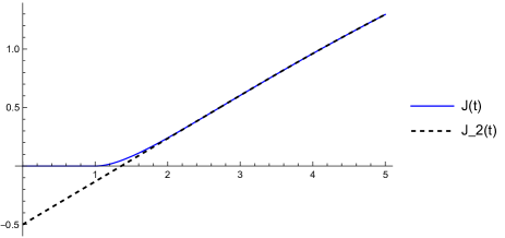
   Figure 1: $J(t)$ and $J_{2}(t)$

4. If $X\sim\text{Weibull}(\lambda,s)$, then $\mathbb{P}\left({\mathinner{\!\left\lvert X\right\rvert}>t}\right)=\exp\left({-(\frac{t}{\lambda})^{s}}\right)$. Hence, one can take the trivial tail bound $J(t)=-\log\mathbb{P}\left({X>t}\right)=\left(\frac{t}{\lambda}\right)^{s}$. This function satisfies $J(0)=0$, and is concave for $s\leq 1$. Hence, Lemma 2.16 yeilds $J(t_{1}+t_{2})\leq J(t_{1})+J(t_{2})$.

5. Let $X\sim\text{Log-logistic}(\alpha,\beta),\;\alpha,\beta>0$

   $$J(t)=-\log\mathbb{P}\left({\mathinner{\!\left\lvert X\right\rvert}>t}\right)=-\log(1-\frac{1}{1+(x/\alpha)^{-\beta}})=\log(1+(x/\alpha)^{\beta}).$$

   Note that

   $$2^{\beta}(1+x^{\beta})(1+y^{\beta})\geq 2^{\beta}+(2\max\{x,y\})^{\beta}\geq 1+(x+y)^{\beta},\quad\forall x,y\geq 1.$$

   therefore

   $$2^{\beta}(1+(t_{1}/\alpha)^{\beta})(1+(t_{2}/\alpha)^{\beta})\geq(1+((t_{1}+t_{2})/\alpha)^{\beta}).$$

   Applying $\log$ to the above inequality yields $J(t_{1})+J(t_{2})+\beta\log 2\geq J(t_{1}+t_{2})$.

6. Let $X\sim\text{Pareto}(x_{m},\alpha)$. Then,

   $$J(t)=-\log\mathbb{P}\left({X>t}\right)=\alpha\log\frac{t}{x_{m}},\quad t>x_{m},$$

   is a concave function on the support of $X$, i.e. $[x_{m},\infty)$. Similar to the Log-Normal case above, one can linearly extend $J(t)$ to a concave function on $[0,\infty)$ and utilize Lemma 2.16 to verify $J(t)$ is shifted sub-additive.

$\square$

4.3 Proof of Lemma 2.19

Proof.

1. The strategy to show (2.10) is to show $\lim\frac{-\log\mathbb{P}\left({\varphi_{n}(X)>\frac{n}{m}t}\right)}{J(kt)}=\lim\frac{I(kt)}{J(kt)}=1$ as $n\to\infty$. Let us write $c\triangleq\mathbb{E}\mathinner{\left[\mathinner{\!\left\lvert X-Y\right\rvert}\right]}$. Note that

$$\varphi_{n}(X) =\inf_{\mathinner{\!\left\lvert y\right\rvert}\leq J^{-1}(\log{2n})}\mathinner{\!\left\lvert X-y\right\rvert}-c$$

$$=\begin{cases}-c&\mbox{if}\ \mathinner{\!\left\lvert X\right\rvert}\leq J^{-1}(\log{2n})\\ \mathinner{\!\left\lvert X\right\rvert}-J^{-1}(\log{2n})-c&\mbox{if}\ \mathinner{\!\left\lvert X\right\rvert}>J^{-1}(\log{2n}).\end{cases}.$$

With the above display in mind, observe that

$$\mathbb{P}(\varphi_{n}(X)>\frac{n}{m}t) =\mathbb{P}\left({\mathinner{\!\left\lvert X\right\rvert}>\frac{n}{m}t+J^{-1}(\log 2n)+c}\right).$$

Note that, by Assumption 2 we have:

$$\lim\limits_{n\to\infty}\frac{-\log\mathbb{P}(\mathinner{\!\left\lvert X\right\rvert}>\frac{n}{m}t+J^{-1}(\log{2n})+c)}{J(\frac{n}{m}t+J^{-1}(\log 2n)+c)}=1.$$

Also, note that for large $n$, $J(kt)\leq J(\frac{n}{m}t+J^{-1}(\log 2n)+c)\leq J(kt+t+J^{-1}(\log 4km)+c)$. Using (4.16) from Lemma 4.2 with $u=4km,\;c_{1}=\frac{t}{4m},\;c_{2}=c+t$ we obtain $\lim\limits_{n\to\infty}\frac{J(kt+t+J^{-1}(\log 4km)+c)}{J(kt)}=1$, therefore

$$\lim\limits_{n\to\infty}\frac{-\log{\mathbb{P}(\varphi_{n}(X)>\frac{n}{m}t)}}{J(kt)}=\lim\limits_{n\to\infty}\frac{J(\frac{n}{m}t+J^{-1}(\log 2n)+c)}{J(kt)}=1.$$ (4.2)

Next, we try to approximate the term $I(kt)$ from (2.10). Towards this direction, we begin by observing that

$$\mathbb{P}(|X_{1}-X_{2}|\geq c+kt)\geq\mathbb{P}(X_{2}\leq c^{\prime})\mathbb{P}(X_{1}\geq c^{\prime}+c+kt),$$

for some $c^{\prime}\in\mathbb{R}$ such that $\mathbb{P}\left({X_{2}\leq c^{\prime}}\right)>0$. Consequently,

$$\limsup\limits_{n\to\infty}\frac{-\log{\mathbb{P}(h(X_{1},X_{2})\geq kt)}}{J(kt+c^{\prime}+c)}\leq 1,$$

Hence,

$$\limsup\limits_{n\to\infty}\frac{I(kt)}{J(kt+c^{\prime}+c)}=\limsup\limits_{n\to\infty}\frac{I(kt)}{J(kt)}\leq 1.$$ (4.3)

We used Lemma 4.2 to drop $c^{\prime}+c$.

For the other direction, we need to establish an upper bound for $\mathbb{P}\left({h(X_{1},X_{2})>kt}\right)$. Let $u>0$, then

$$\mathbb{P}(|X_{1}-X_{2}|\geq u) \leq\mathbb{P}\left({\mathinner{\!\left\lvert X_{1}\right\rvert}>u}\right)+\mathbb{P}\left({\mathinner{\!\left\lvert X_{2}\right\rvert}>u}\right)+\mathbb{P}\left({\mathinner{\!\left\lvert X_{1}-X_{2}\right\rvert}\geq u,\;\mathinner{\!\left\lvert X_{1}\right\rvert},\mathinner{\!\left\lvert X_{2}\right\rvert}\leq u}\right)$$

$$\leq 2\exp\left({-J(u)}\right)+2\mathbb{P}\left({X_{1}>X_{2}+u,\;\mathinner{\!\left\lvert X_{1}\right\rvert},\mathinner{\!\left\lvert X_{2}\right\rvert}\leq u}\right)$$

$$\leq 2\exp\left({-J(u)}\right)+2\sum_{i=0}^{\lceil u\rceil}\mathbb{P}\left({-\frac{i}{\lceil u\rceil}u\leq X_{2}\leq-\frac{i-1}{\lceil u\rceil}u}\right)\mathbb{P}\left({X_{1}\geq(1-\frac{i}{{\lceil u\rceil}})u}\right)$$

$$\leq 2\exp\left({-J(u)}\right)+2\sum_{i=0}^{\lceil u\rceil}\exp\left({-J\left({\frac{i-1}{\lceil u\rceil}u}\right)-J\left({(1-\frac{i}{{\lceil u\rceil}})u}\right)}\right)$$

$$\overset{*}{\leq}2\exp\left({-J(u)}\right)+2\sum_{i=0}^{\lceil u\rceil}\exp\left({-J\left({u-\frac{u}{\lceil u\rceil}}\right)+b}\right)$$

$$\leq 2\exp\left({-J(u)}\right)+2(u+2)\exp\left({b}\right)\exp\left({-J(u-1)}\right)$$

$$\leq 3{\rm e}^{b}u\exp\left({-J(u-1)}\right),\quad\text{for }u\geq 2{\rm e}^{-b}+4.$$

To obtain inequality marked by $*$, we used Assumption 5. Taking $-\log$ of above inequality we get

$$\liminf_{u\to\infty}\frac{-\log\mathbb{P}\left({\mathinner{\!\left\lvert X_{1}-X_{2}\right\rvert}>u}\right)}{-\log 3u-b+J(u-1)}\geq 1.$$ (4.4)

Set $u=kt+c$. Since, by Lemma 4.2, $\lim\limits_{k\to\infty}\frac{-\log 3(kt+c)-b+J(kt+c-1)}{J(kt)}=1$, we obtain:

$$\liminf_{u\to\infty}\frac{I(kt)}{J(kt)}\geq 1.$$ (4.5)

Equations (4.2), (4.3), and (4.5) yield (2.10).

2. Once again, we set $c\triangleq\mathbb{E}(X-Y)^{2}$ and note that, in this case,

$$\varphi_{n}(X) =\inf_{\mathinner{\!\left\lvert y\right\rvert}\leq J^{-1}(\log{2n})}(X-y)^{2}-c$$

$$=\begin{cases}-c&\mbox{if}\ \mathinner{\!\left\lvert X\right\rvert}\leq J^{-1}(\log{2n}),\\ (\mathinner{\!\left\lvert X\right\rvert}-J^{-1}(\log{2n}))^{2}-c&\mbox{if}\ \mathinner{\!\left\lvert X\right\rvert}>J^{-1}(\log{2n}).\end{cases}$$

With the above display in mind, observe that

$$\mathbb{P}(\varphi_{n}(X)>\frac{n}{m}t) =\mathbb{P}(\mathinner{\!\left\lvert X\right\rvert}>J^{-1}(\log{2n})+\sqrt{c+\frac{n}{m}t}).$$

Note that for large enough $n$

$$\sqrt{kt}\leq J^{-1}(\log{2n})+\sqrt{c+\frac{n}{m}t}\leq J^{-1}(\log{2n})+\sqrt{\mathinner{\!\left\lvert c\right\rvert}}+\sqrt{t}+\sqrt{kt}.$$

Hence, by Assumptions 5, 6 we obtain

$$\lim\limits_{n\to\infty}\frac{J(J^{-1}(\log{2n})+\sqrt{c+\frac{n}{m}t})}{J(\sqrt{kt})}=1.$$

(see proof of Lemma 4.2 for details.)

We therefore have

$$\lim\limits_{n\to\infty}\frac{-\log{\mathbb{P}(\varphi_{n}(X)>\frac{n}{m}t)}}{J(\sqrt{kt})}=1.$$ (4.6)

Next, we try to approximate the term $I(kt)$ from (2.10). Note that

$$\mathbb{P}((X_{1}-X_{2})^{2}\geq c+kt)=\mathbb{P}(\mathinner{\!\left\lvert X_{1}-X_{2}\right\rvert}\geq\sqrt{c+kt})\geq\mathbb{P}(\mathinner{\!\left\lvert X_{2}\right\rvert}\leq c^{\prime})\mathbb{P}(\mathinner{\!\left\lvert X_{1}\right\rvert}\geq c^{\prime}+\sqrt{c+kt}),$$ (4.7)

for a constant $c^{\prime}$ such that $\mathbb{P}\left({\mathinner{\!\left\lvert X_{2}\right\rvert}\leq c^{\prime}}\right)>0$. Consequently,

$$\limsup\limits_{n\to\infty}\frac{-\log{\mathbb{P}((X_{1}-X_{2})^{2}\geq c+kt)}}{J(c^{\prime}+\sqrt{c+kt})}\leq 1,$$

which in turn yields

$$\limsup\limits_{n\to\infty}\frac{I(kt)}{J(\sqrt{kt})}\leq 1.$$ (4.8)

We utilized Lemma 4.2 to drop $c,c^{\prime}$ from denominator in limits.

For the other direction, we need to establish an upper bound for the left hand side of (4.7). As proved in (4.4), with $u=\sqrt{c+kt}$, we have

$$\liminf_{k\to\infty}\frac{-\log\mathbb{P}\left({\mathinner{\!\left\lvert X_{1}-X_{2}\right\rvert}>\sqrt{c+kt}}\right)}{-\log 3\sqrt{c+kt}-b+J(\sqrt{c+kt}-1)}\geq 1.$$ (4.9)

Since $\frac{\log\sqrt{c+kt}}{J(\sqrt{kt})}\to 0,\;\frac{J(\sqrt{c+kt}-1)}{J(\sqrt{kt})}\to 1$ as $k\to\infty$, from (4.9) we obtain

$$\liminf_{k\to\infty}\frac{-\log\mathbb{P}\left({h(X_{1},X_{2})\geq kt}\right)}{J(\sqrt{kt})}\geq 1.$$ (4.10)

This completes the proof.

3. We write $c=\mathbb{E}\max(\mathinner{\!\left\lvert X_{1}\right\rvert},...,\mathinner{\!\left\lvert X_{m}\right\rvert})$. Note that

$$\varphi_{n}(X)=\mathinner{\!\left\lvert X\right\rvert}-c.$$

Hence, $\mathbb{P}\left({\varphi_{n}(X)\geq\frac{n}{m}t}\right)=\mathbb{P}\left({\mathinner{\!\left\lvert X\right\rvert}\geq\frac{n}{m}t+c}\right)$, and similar to the above cases we can show:

$$\lim_{n\to\infty}\frac{-\log\mathbb{P}\left({\varphi_{n}(X)\geq\frac{n}{m}t}\right)}{J(kt)}=\lim_{n\to\infty}\frac{I(kt)}{J(kt)}=\lim_{n\to\infty}\frac{-\log\mathbb{P}\left({\varphi_{n}(X)\geq\frac{n}{m}t}\right)}{I(kt)}=1.$$ (4.11)

4. Assume $n$ is large enough so $1\leq J^{-1}(\log 2n)$. Calling $\mathbb{E}\mathinner{\left[X^{2}\right]}-\mathbb{E}\mathinner{\left[\max\mathinner{\left\{X,Y\right\}}\right]}=c$ we have

$$\varphi_{n}(X)=\begin{cases}\frac{1}{2}X^{2}-X-c,&\mbox{if}\ X>\frac{1}{2},\\ \frac{1}{2}X^{2}-\frac{1}{2}-c,&\mbox{if}\ X\leq\frac{1}{2}.\end{cases}$$

Therefore,

$$\mathbb{P}\left({\varphi_{n}(X)>\frac{n}{m}t}\right) =\mathbb{P}\left({\frac{X^{2}}{2}-X>\frac{n}{m}t+c,X>0}\right)+\mathbb{P}\left({X\leq-\sqrt{\frac{2n}{m}t+2c+1}}\right)$$

$$=\mathbb{P}\left({X>1+\sqrt{\frac{2n}{m}t+2c+1}}\right)+\mathbb{P}\left({X\leq-\sqrt{\frac{2n}{m}t+2c+1}}\right).$$

Hence,

$$\mathbb{P}\left({\mathinner{\!\left\lvert X\right\rvert}>\sqrt{\frac{2n}{m}t+2c+1}+1}\right)\leq\mathbb{P}\left({\varphi_{n}(X)>\frac{n}{m}t}\right)\leq\mathbb{P}\left({\mathinner{\!\left\lvert X\right\rvert}>\sqrt{\frac{2n}{m}t+2c+1}}\right).$$

Similar to the previous cases above, by Lemma 4.2, we can then show

$$\lim_{n\to\infty}\frac{-\log\mathbb{P}\left({\varphi_{n}(X)>\frac{n}{m}t}\right)}{J\left(\sqrt{\frac{2n}{m}t+2c+1}+1\right)}=\lim_{n\to\infty}\frac{-\log\mathbb{P}\left({\varphi_{n}(X)>\frac{n}{m}t}\right)}{J\left(\sqrt{\frac{2n}{m}t+2c+1}\right)}=\lim_{n\to\infty}\frac{-\log\mathbb{P}\left({\varphi_{n}(X)>\frac{n}{m}t}\right)}{J(\sqrt{2kt})}=1.$$ (4.12)

Moreover, since $h(X,Y)\geq\min(\frac{1}{2}X^{2}-\frac{1}{2},\frac{1}{2}X^{2}-X)-c$, we obtain

$$\mathbb{P}\left({h(X,Y)>kt}\right) \geq\mathbb{P}\left({\min(\frac{1}{2}X^{2}-\frac{1}{2},\frac{1}{2}X^{2}-X)>kt+c}\right)$$

$$\geq\mathbb{P}\left({\mathinner{\!\left\lvert X\right\rvert}>\sqrt{2kt+2c+1}+1}\right).$$

Hence,

$$\limsup_{n\to\infty}\frac{-\log\mathbb{P}\left({h(X,Y)>kt}\right)}{J(\sqrt{2kt+2c+1}+1)}=\limsup_{n\to\infty}\frac{I(kt)}{J(\sqrt{2kt})}\leq 1.$$ (4.13)

Again, for dropping extra constants from the denominator we used Lemma 4.2.

Furthermore, $h(X,Y)\leq\frac{1}{2}X^{2}+\mathinner{\!\left\lvert X\right\rvert}+\frac{1}{2}Y^{2}+\mathinner{\!\left\lvert Y\right\rvert}-c$, and $\frac{1}{2}X^{2}+\mathinner{\!\left\lvert X\right\rvert}>u\iff\mathinner{\!\left\lvert X\right\rvert}>-1+\sqrt{2u+1},\;\forall u\geq 0$. Hence,

$$\mathbb{P}\left({h(X,Y)>kt}\right) \leq\mathbb{P}\left({\frac{1}{2}X^{2}+\mathinner{\!\left\lvert X\right\rvert}+\frac{1}{2}Y^{2}+\mathinner{\!\left\lvert Y\right\rvert}>kt+c}\right)$$

$$\leq\mathbb{P}\left({\frac{1}{2}X^{2}+\mathinner{\!\left\lvert X\right\rvert}>kt+c}\right)+\mathbb{P}\left({\frac{1}{2}Y^{2}+\mathinner{\!\left\lvert Y\right\rvert}>kt+c}\right)$$

$$\quad+\sum_{i=1}^{\lceil kt+c\rceil}\mathbb{P}\left({\frac{i-1}{{\lceil kt+c\rceil}}(kt+c)\leq\frac{1}{2}X^{2}+\mathinner{\!\left\lvert X\right\rvert}\leq\frac{i}{{\lceil kt+c\rceil}}(kt+c)}\right)\times$$

$$\hskip 56.9055pt\mathbb{P}\left({\frac{1}{2}Y^{2}+\mathinner{\!\left\lvert Y\right\rvert}>(1-\frac{i}{{\lceil kt+c\rceil}})(kt+c)}\right)$$

$$\leq 2\mathbb{P}\left({\mathinner{\!\left\lvert X\right\rvert}>-1+\sqrt{2kt+2c+1}}\right)$$

$$\quad+\sum_{i=1}^{\lceil kt+c\rceil}\mathbb{P}\left({\mathinner{\!\left\lvert X\right\rvert}\geq-1+\sqrt{\frac{2(i-1)}{{\lceil kt+c\rceil}}(kt+c)+1}}\right)\times$$

$$\hskip 56.9055pt\mathbb{P}\left({\mathinner{\!\left\lvert Y\right\rvert}>-1+\sqrt{2(1-\frac{i}{{\lceil kt+c\rceil}})(kt+c)+1}}\right)$$

$$\leq 2\exp\left({-J(-1+\sqrt{2kt+2c+1})}\right)$$

$$\quad+\sum_{i=1}^{\lceil kt+c\rceil}\exp\left({-J(-1+\sqrt{\frac{2(i-1)}{{\lceil kt+c\rceil}}(kt+c)+1})-J(-1+\sqrt{2(1-\frac{i}{{\lceil kt+c\rceil}})(kt+c)+1})}\right)$$

$$\overset{*}{\leq}2\exp\left({-J(-1+\sqrt{2kt+2c+1})}\right)+\sum_{i=1}^{\lceil kt+c\rceil}{\rm e}^{b}\exp\left({-J(-2+\sqrt{2(1-\frac{1}{\lceil kt+c\rceil})(kt+c)+2})}\right)$$

$$=2\exp\left({-J(-1+\sqrt{2kt+2c+1})}\right)+{\lceil kt+c\rceil}{\rm e}^{b}\exp\left({-J(-2+\sqrt{2(1-\frac{1}{\lceil kt+c\rceil})(kt+c)+2})}\right).$$

To obtain inequality marked by $*$ we used Assumption 5 and the fact that $\sqrt{x+y}\leq\sqrt{x}+\sqrt{y}$ for non-negative $x,y$.

Hence, by Lemma 4.3 we obtain

$$\liminf_{n\to\infty}\frac{I(kt)}{J(\sqrt{2kt})}\geq 1,$$ (4.14)

which concludes the proof. $\square$

Lemma 4.2.

If tail function $J(t)$, defined in (2.2), satisfy Assumptions 5, 6, then for any $c_{1}>0$ and $c_{2},c_{3}\in\mathbb{R}$ we have

$$\lim_{u\to\infty}\frac{J(u+c_{2})}{J(u)}=1$$ (4.15)

$$\lim_{u\to\infty}\frac{J(c_{1}u+J^{-1}(\log u)+c_{2})}{J(c_{1}u)}=1$$ (4.16)

$$\lim_{u\to\infty}\frac{J(c_{2}+\sqrt{u+c}_{3})}{J(\sqrt{u})}=1$$ (4.17)

Proof.

To prove (4.15), one only need to note that by Assumption 5 we have

$$J(u)-J(\mathinner{\!\left\lvert c_{2}\right\rvert})-b\leq J(u-\mathinner{\!\left\lvert c_{2}\right\rvert})\leq J(u+c_{2})\leq J(u+\mathinner{\!\left\lvert c_{2}\right\rvert})\leq J(u)+J(\mathinner{\!\left\lvert c_{2}\right\rvert})+b,$$ (4.18)

and that $J$ is a non-decreasing function, and $J(u)\xrightarrow{u\to\infty}\infty$.

To show (4.16) observe that $J^{-1}(\log u)+c_{2}>0$ for large enough $u$. By Assumption 5 we obtain

$$J(c_{1}u)\leq J(c_{1}u+J^{-1}(\log u)+c_{2}) \leq J(c_{1}u)+\log u+J(\mathinner{\!\left\lvert c_{2}\right\rvert})+2b.$$

Note that $\lim\frac{\log u}{J(u)}=\lim\frac{C}{J(u)}=0$ as $u\to\infty$, so dividing by $J(c_{1}u)$ and taking limit of the above inequalities yields (4.16).

For the third part observe that when $u$ is large enough we have

$$\sqrt{u}-\sqrt{\mathinner{\!\left\lvert c_{3}\right\rvert}}-\mathinner{\!\left\lvert c_{2}\right\rvert}\leq c_{2}+\sqrt{u+c_{3}}\leq\sqrt{u}+\sqrt{\mathinner{\!\left\lvert c_{3}\right\rvert}}+\mathinner{\!\left\lvert c_{2}\right\rvert}.$$

Then, since $J$ is non-decreasing and satisfies Assumption 5 we obtain

$$J(\sqrt{u})-J(\sqrt{\mathinner{\!\left\lvert c_{3}\right\rvert}}+\mathinner{\!\left\lvert c_{2}\right\rvert})-b\leq J(c_{2}+\sqrt{u+c_{3}})\leq J(\sqrt{u})+J(\sqrt{\mathinner{\!\left\lvert c_{3}\right\rvert}}+\mathinner{\!\left\lvert c_{2}\right\rvert})+b.$$

Once again, dividing by $J(\sqrt{u})$ and taking $u\to\infty$ yields (4.17). $\square$

Lemma 4.3.

Under Assumptions 5, 6 we have

$$\lim_{k\to\infty}\frac{-\log\left(2\exp\left({-J(-1+\sqrt{2kt+2c+1})}\right)+{\lceil kt+c\rceil}{\rm e}^{b}\exp\left({-J(-2+\sqrt{2(1-\frac{1}{\lceil kt+c\rceil})(kt+c)+2})}\right)\right)}{J(\sqrt{2kt})}=1$$

Proof.

Given Lemma 4.1, it suffices to show that

$$\lim_{k\to\infty}\frac{-\log\left(2\exp\left({-J(-1+\sqrt{2kt+2c+1})}\right)\right)}{J(\sqrt{2kt})}=1$$ (4.19)

$$\lim_{k\to\infty}\frac{-b-\log\left({\lceil kt+c\rceil}\exp\left({-J(-2+\sqrt{2(1-\frac{1}{\lceil kt+c\rceil})(kt+c)+2})}\right)\right)}{J(\sqrt{2kt})}=1.$$ (4.20)

Note that

$$\lim_{k\to\infty}\frac{-\log\left(2\exp\left({-J(-1+\sqrt{2kt+2c+1})}\right)\right)}{J(\sqrt{2kt})} =\lim_{k\to\infty}\frac{J(-1+\sqrt{2kt+2c+1})}{J(\sqrt{2kt})}=1,$$

by Lemma 4.2.

Moreover,

$$\lim_{k\to\infty}\frac{-b-\log\left({\lceil kt+c\rceil}\exp\left({-J(-2+\sqrt{2(1-\frac{1}{\lceil kt+c\rceil})(kt+c)+2})}\right)\right)}{J(\sqrt{2kt})}$$

$$\;=\lim_{k\to\infty}\frac{-b-\log\lceil kt+c\rceil}{J(\sqrt{2kt})}+\frac{J(-2+\sqrt{2(1-\frac{1}{\lceil kt+c\rceil})(kt+c)+2})}{J(\sqrt{2kt})}.$$

By Assumption 6 we have $\lim\limits_{k\to\infty}\frac{-b-\log\lceil kt+c\rceil}{J(\sqrt{2kt})}=\lim\limits_{k\to\infty}\frac{-2\log\sqrt{\lceil kt+c\rceil}}{J(\sqrt{2kt})}=0$. We also have

$$\lim_{k\to\infty}\sqrt{2(1-\frac{1}{\lceil kt+c\rceil})(kt+c)+2}=\sqrt{2kt+2c+2},$$

Hence, for large enough $k$, there are fixed $c_{2},c_{3}\in\mathbb{R}$ such that

$$-2+\sqrt{2kt+c_{2}}\leq-2+\sqrt{2(1-\frac{1}{\lceil kt+c\rceil})(kt+c)+2}\leq-2+\sqrt{2kt+c_{3}},\quad\forall k>K.$$

Given $J(t)$ is an increasing function, and $\lim_{k\to\infty}\frac{J(-2+\sqrt{2kt+c_{i}})}{J(\sqrt{2kt})}=1,\;i=2,3$ by Lemma 4.2 we obtain

$$\lim_{k\to\infty}\frac{J(-2+\sqrt{2(1-\frac{1}{\lceil kt+c\rceil})(kt+c)+2})}{J(\sqrt{2kt})}=1.$$ (4.21)

$\square$

References

- Arcones [1992] Miguel A Arcones. Large deviations for u-statistics. Journal of multivariate analysis, 42(2):299–301, 1992.
- Bakhshizadeh et al. [2020] Milad Bakhshizadeh, Arian Maleki, and Victor H. de la Pena. Sharp concentration results for heavy-tailed distributions, 2020. URL https://arxiv.org/abs/2003.13819.
- Baringhaus and Rank [2002] L Baringhaus and R Rank. On large deviations of u-statistics and their projections. Sankhyā: The Indian Journal of Statistics, Series A, pages 167–170, 2002.
- Bretagnolle [1999] Jean Bretagnolle. A new large deviation inequality for u-statistics of order 2. ESAIM: Probability and Statistics, 3:151–162, 1999.
- Chakrabortty and Kuchibhotla [2018] Abhishek Chakrabortty and Arun Kumar Kuchibhotla. Tail bounds for canonical u-statistics and u-processes with unbounded kernels. 2018.
- Dasgupta [1984] Ratan Dasgupta. On large deviation probabilities of u-statistics in non iid case. Sankhyā: The Indian Journal of Statistics, Series A, pages 110–116, 1984.
- de la Pena [1992] Victor H de la Pena. Decoupling and khintchine’s inequalities for u-statistics. The Annals of Probability, pages 1877–1892, 1992.
- Eichelsbacher [2005] Peter Eichelsbacher. Refined large deviations for von mises statistics. Theory of Probability & Its Applications, 49(1):139–148, 2005.
- Eichelsbacher and Löwe [1995] Peter Eichelsbacher and Matthias Löwe. A large deviation principle form-variate von mises-statistics and u-statistics. Journal of Theoretical Probability, 8(4):807–824, 1995.
- Fan et al. [2012] Xiequan Fan, Ion Grama, and Quansheng Liu. Large deviation exponential inequalities for supermartingales. Electronic Communications in Probability, 17:1–8, 2012.
- Giné et al. [2000] Evarist Giné, Rafał Latała, and Joel Zinn. Exponential and moment inequalities for u-statistics. In High Dimensional Probability II, pages 13–38. Springer, 2000.
- Hoeffiding [1948] W Hoeffiding. A class of statistics with asymptotically normal distributions. Annals of Mathematical Statistics, 19:293–325, 1948.
- Houdré and Reynaud-Bouret [2003] Christian Houdré and Patricia Reynaud-Bouret. Exponential inequalities, with constants, for u-statistics of order two. In Stochastic inequalities and applications, pages 55–69. Springer, 2003.
- Kiessling and Wang [2012] Michael K-H Kiessling and Yu Wang. Onsager’s ensemble for point vortices with random circulations on the sphere. Journal of Statistical Physics, 148(5):896–932, 2012.
- Korolyuk and Borovskich [2013] Vladimir S Korolyuk and Yu V Borovskich. Theory of U-statistics, volume 273. Springer Science & Business Media, 2013.
- Lee [2019] A.J. Lee. U-Statistics: Theory and Practice. CRC Press, 2019. ISBN 9781351405850. URL https://books.google.com/books?id=YC2NDwAAQBAJ.
- Liu and Wu [2020] Wei Liu and Liming Wu. Large deviations for empirical measures of mean-field gibbs measures. Stochastic Processes and their Applications, 130(2):503–520, 2020.
- Nikitin and Ponikarov [2001] Ya. Yu. Nikitin and E.V. Ponikarov. Rough asymptotics of probabilities of chernoff type large deviations for von mises functionals and u-statistics. Translations of the American Mathematical Society-Series 2, 203:107–146, 2001.
- Nikitin [1995] Yakov Nikitin. Asymptotic efficiency of nonparametric tests. Cambridge University Press, 1995.
- Talagrand [1996] Michel Talagrand. New concentration inequalities in product spaces. Inventiones mathematicae, 126(3):505–563, 1996.
- Vershynin [2018] Roman Vershynin. High-dimensional probability: An introduction with applications in data science, volume 47. Cambridge university press, 2018.
- Wang [1994] Wenyang Wang. Large deviations of U-empirical probability measures and statistical functionals. The Johns Hopkins University, 1994.
- Yakov Y Nikitin [2004] Irina Peaucelle Yakov Y Nikitin. Efficiency and local optimality of nonparametric tests based on u-and v-statistics. Metron, 62(2):185–200, 2004.