Accelerating Guided Diffusion Sampling with Splitting Numerical Methods

Abstract

Guided diffusion is a technique for conditioning the output of a diffusion model at sampling time without retraining the network for each specific task. One drawback of diffusion models, however, is their slow sampling process. Recent techniques can accelerate unguided sampling by applying high-order numerical methods to the sampling process when viewed as differential equations. On the contrary, we discover that the same techniques do not work for guided sampling, and little has been explored about its acceleration. This paper explores the culprit of this problem and provides a solution based on operator splitting methods, motivated by our key finding that classical high-order numerical methods are unsuitable for the conditional function. Our proposed method can re-utilize the high-order methods for guided sampling and can generate images with the same quality as a 250-step DDIM baseline using 32-58% less sampling time on ImageNet256. We also demonstrate usage on a wide variety of conditional generation tasks, such as text-to-image generation, colorization, inpainting, and super-resolution.

1 Introduction

A family of generative models known as diffusion models has recently gained a lot of attention with state-of-the-art image generation quality (Dhariwal & Nichol, 2021). Guided diffusion is an approach for controlling the output of a trained diffusion model for conditional generation tasks without retraining its network. By engineering a task-specific conditional function and modifying only the sampling procedure, guided diffusion models can be used in a variety of applications, such as class-conditional image generation (Dhariwal & Nichol, 2021; Kawar et al., 2022), text-to-image generation (Nichol et al., 2022), image-to-image translation (Zhao et al., 2022), inpainting (Chung et al., 2022a), colorization (Song et al., 2020b), image composition (Sasaki et al., 2021), adversarial purification (Wang et al., 2022; Wu et al., 2022) and super-resolution (Choi et al., 2021).

One common drawback of both guided and regular “unguided” diffusion models is their slow sampling processes, usually requiring hundreds of iterations to produce a single image. Recent speed-up attempts include improving the noise schedule (Nichol & Dhariwal, 2021; Watson et al., 2021), redefining the diffusion process to be non-Markovian, thereby allowing a deterministic sampling process Song et al. (2020a), network distillation that teaches a student model to simulate multiple sampling steps of a teacher model Salimans & Ho (2022); Luhman & Luhman (2021), among others. Song et al. (2020a) show how each sampling step can be expressed as a first-order numerical step of an ordinary differential equation (ODE). Similarly, Song et al. (2020b) express the sampling of a score-based model as solving a stochastic differential equation (SDE). By regarding the sampling process as an ODE/SDE, many high-order numerical methods have been suggested, such as Liu et al. (2022), Zhang & Chen (2022), and Zhang et al. (2022) with impressive results on unguided diffusion models. However, when applied to guided diffusion models, these methods produce surprisingly poor results (see Figure 1)—given a few number of steps, those high-order numerical methods actually perform worse than low-order methods.

Guided sampling differs from the unguided one by the addition of the gradients of the conditional function to its sampling equation. The observed performance decline thus suggests that classical high-order methods may not be suitable for the conditional function and, consequently, the guided sampling equation as a whole. Our paper tests this hypothesis and presents an approach to accelerating guided diffusion sampling. The key idea is to use an operator splitting method to split the less well-behaved conditional function term from the standard diffusion term and solve them separately. This approach not only allows re-utilizing the successful high-order methods on the diffusion term but also provides us with options to combine different specialized methods for each term to maximize performance. Splitting method can be used to solve diffusion SDE in Dockhorn et al. (2021).

Our design process includes comparing different splitting methods and numerical methods for each split term. When tested on ImageNet, our approach achieves the same level of image quality as a DDIM baseline while reducing the sampling time by approximately 32-58%. Compared with other sampling methods using the same sampling time, our approach provides better image quality as measured by LPIPS, FID, and Perception/Recall. With only minimal modifications to the sampling equation, we also show successful acceleration on various conditional generation tasks.

Number of steps	8       16     32     64     128    256
DDIM
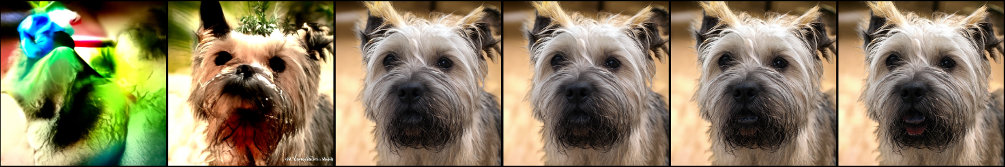
PLMS4
STSP4 (Ours)

Figure 1: Generated samples of a classifier-guided diffusion model trained on ImageNet256 using 8-256 sampling steps from different sampling methods. Our technique, STSP4, produces high-quality results in a fewer number of steps.

2 Background

This section provides a high-level summary of the theoretical foundation of diffusion models as well as numerical methods that have been used for diffusion models. Here we briefly explain a few that contribute to our method.

2.1 Diffusion Models

Assuming that $x_{0}$ is a random variable from the data distribution we wish to reproduce, diffusion models define a sequence of Gaussian noise degradation of $x_{0}$ as random variables $x_{1},x_{2},...,x_{T}$, where $x_{t}\sim\mathcal{N}(\sqrt{1-\beta_{t}}x_{t-1},\beta_{t}\mathbf{I})$ and $\beta_{t}\in[0,1]$ are parameters that control the noise levels. With a property of Gaussian distribution, we can express $x_{t}$ directly as a function of $x_{0}$ and noise $\epsilon\sim\mathcal{N}(0,\mathbf{I})$ by $x_{t}=\sqrt{\bar{\alpha}_{t}}x_{0}+\sqrt{1-\bar{\alpha}_{t}}\epsilon$, where $\bar{\alpha}_{t}=\prod^{t}_{i=1}(1-\beta_{i})$. By picking a sufficiently large $T$ (e.g., 1,000) and an appropriate set of $\beta_{t}$, we can assume $x_{T}$ is a standard Gaussian distribution. The main idea of diffusion model generation is to sample a Gaussian noise $x_{T}$ and use it to reversely sample $x_{T-1}$, $x_{T-2},...$ until we obtain $x_{0}$, which belongs to our data distribution.

Ho et al. (2020) propose Denoising Diffusion Probabilistic Model (DDPM) and explain how to employ a neural network $\epsilon_{\theta}(x_{t},t)$ to predict the noise $\epsilon$ that is used to compute $x_{t}$. To train the network, we sample a training image $x_{0}$, $t$, and $\epsilon$ to compute $x_{t}$ using the above relationship. Then, we optimize our network $\epsilon_{\theta}$ to minimize the difference between the predicted and real noise, i.e., $\|\epsilon-\epsilon_{\theta}(x_{t},t)\|^{2}$.

Song et al. (2020a) introduce Denoising Diffusion Implicit Model (DDIM), which uses the network $\epsilon_{\theta}$ to deterministically obtain $x_{t-1}$ given $x_{t}$. The DDIM generative process can be written as

$$x_{t-1}=\sqrt{\frac{\bar{\alpha}_{t-1}}{\bar{\alpha}_{t}}}\left(x_{t}-\sqrt{1-\bar{\alpha}_{t}}\epsilon_{\theta}(x_{t},t)\right)+\sqrt{1-\bar{\alpha}_{t-1}}\epsilon_{\theta}(x_{t},t).$$ (1)

This formulation could be used to skip many sampling steps and boost sampling speed. To turn this into an ODE, we rewrite Equation 1 as:

$$\frac{x_{t-\Delta t}}{\sqrt{\bar{\alpha}_{t-\Delta t}}}=\frac{x_{t}}{\sqrt{\bar{\alpha}_{t}}}+\left(\sqrt{\frac{1-\bar{\alpha}_{t-\Delta t}}{\bar{\alpha}_{t-\Delta t}}}-\sqrt{\frac{1-\bar{\alpha}_{t}}{\bar{\alpha}_{t}}}\right)\epsilon_{\theta}(x_{t},t),$$ (2)

which is now equivalent to a numerical step in solving an ODE. To derive the corresponding ODE, we can re-parameterize $\sigma_{t}=\sqrt{1-\bar{\alpha}_{t}}/\sqrt{\bar{\alpha}_{t}},\>\bar{x}(t)=x_{t}/\sqrt{\bar{\alpha}_{t}}$ and $\bar{\epsilon}_{\sigma}(\bar{x})=\epsilon_{\theta}(x_{t},t)$, yielding $\bar{x}({t-\Delta t})-\bar{x}({t})=(\sigma_{t-\Delta t}-\sigma_{t})\bar{\epsilon}_{\sigma}(\bar{x})$. By letting $(\sigma_{t-\Delta t}-\sigma_{t})\rightarrow 0$, the ODE becomes:

$$\frac{d\bar{x}}{d\sigma}=\bar{\epsilon}_{\sigma}(\bar{x}).$$ (3)

Note that this change of variables is equivalent to an exponential integrator technique described in both Zhang & Chen (2022) and Lu et al. (2022). Since $x_{t}$ and $\bar{x}(t)$ have the same value at $t=0$, our work can focus on solving $\bar{x}(t)$ rather than $x_{t}$. Many numerical methods can be applied to the ODE Equation 3 to accelerate diffusion sampling. We next discuss some of them that are relevant.

2.2 Numerical Methods

Euler’s Method is the most basic numerical method. A forward Euler step is given by $\bar{x}_{n+1}=\bar{x}_{n}+\Delta\sigma\bar{\epsilon}_{\sigma}(\bar{x}_{n})$. When we apply the forward Euler step to the ODE Equation 3, we get the DDIM formulation (Song et al., 2020a).

Heun’s Method, also known as the trapezoid rule or improved Euler, is given by: $\bar{x}_{n+1}=\bar{x}_{n}+\frac{\Delta\sigma}{2}(e_{1}+e_{2})$, where $e_{1}=\bar{\epsilon}_{\sigma}(\bar{x}_{n})$ and $e_{2}=\bar{\epsilon}_{\sigma}(\bar{x}_{n}+\Delta\sigma e_{1}).$ This method modifies Euler’s method into a two-step method to improve accuracy. Many papers have used this method on diffusion models, including Algorithm 1 in Karras et al. (2022) and DPM-Solver-2 in Lu et al. (2022). This method is also the simplest case of Predictor-Corrector methods used in Song et al. (2020b).

Runge-Kutta Methods represent a class of numerical methods that integrate information from multiple hidden steps and provide high accuracy results. Heun’s method also belongs to a family of 2^nd-order Runge-Kutta methods (RK2). The most well-known variant is the 4^th-order Runge-Kutta method (RK4), which is written as follows:

$$e_{1}=\bar{\epsilon}_{\sigma}(\bar{x}_{n}),\quad e_{2}=\bar{\epsilon}_{\sigma}\left(\bar{x}_{n}+\frac{\Delta\sigma}{2}e_{1}\right),\quad e_{3}=\bar{\epsilon}_{\sigma}\left(\bar{x}_{n}+\frac{\Delta\sigma}{2}e_{2}\right),\quad e_{4}=\bar{\epsilon}_{\sigma}\left(\bar{x}_{n}+\Delta\sigma e_{3}\right),$$

$$\bar{x}_{n+1}=\bar{x}_{n}+\frac{\Delta\sigma}{6}(e_{1}+2e_{2}+2e_{3}+e_{4}).$$ (4)

This method has been tested on diffusion models in Liu et al. (2022) and Salimans & Ho (2022), but it has not been used as the main proposed method in any paper.

Linear Multi-Step Method, similar to the Runge-Kutta methods, aims to combine information from several steps; however, rather than evaluating new hidden steps, this method uses the previous steps to estimate the new step. The 1^st-order formulation is the same as Euler’s method. The 2^nd-order formulation is given by

$$\bar{x}_{n+1}=\bar{x}_{n}+\frac{\Delta\sigma}{2}\left(3e_{0}-e_{1}\right),$$ (5)

while the 4^th-order formulation is given by

$$\bar{x}_{n+1}=\bar{x}_{n}+\frac{\Delta\sigma}{24}(55e_{0}-59e_{1}+37e_{2}-9e_{3}),$$ (6)

where $e_{k}=\bar{\epsilon}_{\sigma}(\bar{x}_{n-k})$. These formulations are designed for a constant $\Delta\sigma$ in each step. However, our experiments and previous work that uses this method (e.g., Liu et al. (2022); Zhang & Chen (2022)) still show good results when this assumption is not strictly satisfied, i.e., when $\Delta\sigma$ is not constant. We will refer to these formulations as PLMS (Pseudo Linear Multi-Step) for the rest of the paper, like in Liu et al. (2022). A similar linear multi-step method for non-constant $\Delta\sigma$ can also be derived using a technique used in Zhang & Chen (2022), which we detail in Appendix B. The method can improve upon PLMS slightly, but it is not as flexible because we have to re-derive the update rule every time the $\sigma$ schedule changes.

3 Splitting Methods for Guided Diffusion Models

This section introduces our technique that uses splitting numerical methods to accelerate guided diffusion sampling. We first focus our investigation on classifier-guided diffusion models for class-conditional generation and later demonstrate how this technique can be used for other conditional generation tasks in Section 4.3. Like any guided diffusion models, classifier-guided models (Dhariwal & Nichol, 2021) share the same training objective with regular unguided models with no modifications to the training procedure; but the sampling process is guided by an additional gradient signal from an external classifier to generate class-specific output images. Specifically, the sampling process is given by

$$\hat{\epsilon}=\epsilon_{\theta}(x_{t})-\sqrt{1-\bar{\alpha}_{t}}\nabla_{x}\log p_{\phi}(c|x_{t}),\quad x_{t-1}=\sqrt{\bar{\alpha}_{t-1}}\left(\frac{x_{t}-\sqrt{1-\bar{\alpha}_{t}}\hat{\epsilon}}{\sqrt{\bar{\alpha}_{t}}}\right)+\sqrt{1-\bar{\alpha}_{t-1}}\hat{\epsilon},$$ (7)

where $p_{\phi}(c|x_{t})$ is a classifier model trained to output the probability of $x_{t}$ belonging to class $c$. As discussed in the previous section, we can rewrite this formulation as a “guided ODE”:

$$\frac{d\bar{x}}{d\sigma}=\bar{\epsilon}_{\sigma}(\bar{x})-\nabla f_{\sigma}(\bar{x}),$$ (8)

where $f_{\sigma}(\bar{x})=\frac{\sigma}{\sqrt{\sigma^{2}+1}}\log p_{\phi}(c|x_{t})$. We refer to $f_{\sigma}$ as the conditional function, which can be substituted with other functions for different tasks. After obtaining the ODE form, any numerical solver mentioned earlier can be readily applied to accelerate the sampling process. However, we observe that classical high-order numerical methods (e.g., PLMS4, RK4) fail to accelerate this task (see Figure 1) and even perform worse than the baseline DDIM.

We hypothesize that the two terms in the guided ODE may have different numerical behaviors with the conditional term being less suitable to classical high-order methods. We speculate that the difference could be partly attributed to how they are computed: $\nabla f_{\sigma}(\bar{x})$ is computed through backpropagation, whereas $\bar{\epsilon}_{\sigma}(\bar{x})$ is computed directly by evaluating a network. One possible solution to handle terms with different behaviors is the so-called operator splitting method, which divides the problem into two subproblems:

$$\frac{dy}{d\sigma}=\bar{\epsilon}_{\sigma}(y),\quad\frac{dz}{d\sigma}=-\nabla f_{\sigma}(z).$$ (9)

We call these the diffusion and condition subproblems, respectively. This method allows separating the hard-to-approximate $\nabla f_{\sigma}(z)$ from $\bar{\epsilon}_{\sigma}(y)$ and solving them separately in each time step. Importantly, this helps reintroduce the effective use of high-order methods on the diffusion subproblem as well as provides us with options to combine different specialized methods to maximize performance. We explore two most famous first- and second-order splitting techniques for our task:

3.1 Lie-Trotter Splitting (LTSP)

Our first example is the simple first-order Lie-Trotter splitting method (Trotter, 1959), which expresses the splitting as

$$\frac{dy}{d\sigma} =\bar{\epsilon}_{\sigma}(y), y(\sigma_{n}) =\bar{x}_{n}, \sigma\in[\sigma_{n+1},\sigma_{n}]$$ (10)

$$\frac{dz}{d\sigma} =-\nabla f_{\sigma}(z), z(\sigma_{n}) =y(\sigma_{n+1}), \sigma\in[\sigma_{n+1},\sigma_{n}]$$ (11)

with the solution of this step being $\bar{x}_{n+1}=z(\sigma_{n+1})$. Note that $\sigma_{n}$ is a decreasing sequence in sampling schedule. Here Equation 10 is the same as Equation 3, which can be solved using any high-order numerical method, e.g., PLMS. For Equation 11, we can use a forward Euler step:

$$z_{n+1}=z_{n}-\Delta\sigma\nabla f_{\sigma}(z_{n}).$$ (12)

This is equivalent to a single iteration of standard gradient descent with a learning rate $\Delta\sigma$. This splitting scheme is summarized by Algorithm 1. We investigate different numerical methods for each subproblem in Section 4.1.

sample $\bar{x}_{0}\sim\mathcal{N}(0,\sigma^{2}_{\text{max}}\mathbf{I})$ ;

for $n\in\{0,...,N-1\}$ do

       $y_{n+1}=\text{PLMS}(\bar{x}_{n},\sigma_{n},\sigma_{n+1},\bar{\epsilon}_{\sigma})$;

       $\bar{x}_{n+1}=y_{n+1}-(\sigma_{n+1}-\sigma_{n})\nabla f(y_{n+1})$ ;

      

end for

Result: $\bar{x}_{N}$

Algorithm 1 Lie-Trotter Splitting (LTSP)

sample $\bar{x}_{0}\sim\mathcal{N}(0,\sigma^{2}_{\text{max}}\mathbf{I})$ ;

for $n\in\{0,...,N-1\}$ do

       $z_{n+1}=\bar{x}_{n}-\frac{(\sigma_{n+1}-\sigma_{n})}{2}\nabla f(\bar{x}_{n})$ ;

       $y_{n+1}=\text{PLMS}(z_{n+1},\sigma_{n},\sigma_{n+1},\bar{\epsilon}_{\sigma})$;

       $\bar{x}_{n+1}=y_{n+1}-\frac{(\sigma_{n+1}-\sigma_{n})}{2}\nabla f(y_{n+1})$ ;

      

end for

Result: $\bar{x}_{N}$

Algorithm 2 Strang Splitting (STSP)

3.2 Strang Splitting (STSP)

Strang splitting (or Strang-Marchuk) (Strang, 1968) is one of the most famous and widely used operator splitting methods. This second-order splitting works as follows:

$$\frac{dz}{d\sigma} =-\nabla f_{\sigma}(z), z(\sigma_{n})=\bar{x}_{n}, \sigma\in\left[\frac{1}{2}(\sigma_{n}+\sigma_{n+1}),\sigma_{n}\right]$$ (13)

$$\frac{dy}{d\sigma} =\bar{\epsilon}_{\sigma}(y), y(\sigma_{n})=z\left(\frac{1}{2}(\sigma_{n}+\sigma_{n+1})\right), \sigma\in[\sigma_{n+1},\sigma_{n}]$$ (14)

$$\frac{d\tilde{z}}{d\sigma} =-\nabla f_{\sigma}(\tilde{z}), \tilde{z}\left(\frac{1}{2}(\sigma_{n}+\sigma_{n+1})\right)=y(\sigma_{n+1}), \sigma\in\left[\sigma_{n+1},\frac{1}{2}(\sigma_{n}+\sigma_{n+1})\right]$$ (15)

Instead of solving each subproblem for a full step length, we solve the condition subproblem for half a step before and after solving the diffusion subproblem for a full step. In theory, we can swap the order of operations without affecting convergence, but it is practically cheaper to compute the condition term twice rather than the diffusion term twice because $f_{\sigma}$ is typically a smaller network compared to $\bar{\epsilon}_{\sigma}$. The Strange splitting algorithm is shown in Algorithm 2. This method can be proved to have better accuracy than the Lie-Trotter method using the Banker-Campbell-Hausdorff formula (Tuckerman, 2010), but it requires evaluating the condition term twice per step in exchange for improved image quality. We assess this trade-off in the experiment section.

4 Experiments

Extending on our observation that classical high-order methods failed on guided sampling, we conducted a series of experiments to investigate this problem and evaluate our solution. Section 4.1 uses a simple splitting method (first-order LTSP) to study the effects that high-order methods have on each subproblem, leading to our key finding that only the conditional subproblem is less suited to classical high-order methods. This section also determines the best combination of numerical methods for the two subproblems under LTSP splitting. Section 4.2 explores improvements from using a higher-order splitting method and compares our best scheme to previous work. Finally, Section 4.3 applies our approach to a variety of conditional generation tasks with minimal changes.

For our comparison, we use pre-trained state-of-the-art diffusion models and classifiers from Dhariwal & Nichol (2021), which were trained on the ImageNet dataset (Russakovsky et al., 2015) with 1000 total sampling step. We treat full-path samples from a classifier-guided DDIM at 1,000 steps as reference solutions. Then the performance of each configuration is measured by the image similarity between its generated samples using fewer steps and the reference DDIM samples, both starting from the same initial noise maps. Given the same sampling time, we expect configurations with better performance to better match the full DDIM. We measure image similarity using Learned Perceptual Image Patch Similarity (LPIPS) (Zhang et al., 2018) (lower is better) and measure sampling time using a single NVIDIA RTX 3090 and a 24-core AMD Threadripper 3960x.

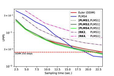
(a) Varying the method for the diffusion subproblem

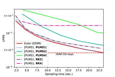
(b) Varying the method for the condition subproblem

Figure 2: Comparison of different combinations of numerical methods under LTSP splitting for guided diffusion sampling. We plot LPIPS against the sampling time. [A, B] denotes the use of method A in the diffusion subproblem and method B in the condition subproblem. The red dotted lines indicate a reference DDIM score obtained from 250 sampling steps, which produce images visually close to those from 1,000 steps.

4.1 Finding a suitable numerical method for each subproblem

To study the effects of different numerical methods on each subproblem of the guided ODE (Equation 8), we use the simplest Lie-Trotter splitting, which itself requires no additional network evaluations. This controlled experiment has two setups: a) we fix the numerical method for the condition subproblem (Equation 11) to first-order PLMS1 (Euler’s method) and vary the numerical method for the diffusion subproblem (Equation 10), and conversely b) we fix the method for the diffusion subproblem and vary the method for the condition subproblem. The numerical method options are Euler’s method (PLMS1), Heun’s method (RK2), 4^th order Runge-Kutta’s method (RK4), and 2^nd/4^th order pseudo linear multi-step (PLMS2/PLMS4). We report LPIPS vs. sampling time of various numerical combinations on a diffusion model trained on ImageNet 256$\times$256 in Figure 2. The red dotted lines indicate a reference DDIM score obtained from 250 sampling steps, a common choice that produces good samples that are perceptually close to those from a full 1,000-step DDIM (Dhariwal & Nichol, 2021; Nichol & Dhariwal, 2021).

Given a long sampling time, non-split PLMS4 performs better than the DDIM baseline. However, when the sampling time is reduced, the image quality of PLMS4 rapidly decreases and becomes much worse than that of DDIM, especially under 15 seconds in Figure 2. When we split the ODE and solve both subproblems using first-order PLMS1 (Euler), the performance is close to that of DDIM, which is also considered first-order but without any splitting. This helps verify that merely splitting the ODE does not significantly alter the sampling speed.

In the setup a), when RK2 and RK4 are used for the diffusion subproblem, they also perform worse than the DDIM baseline. This slowdown is caused by the additional evaluations of the network by these methods, which outweigh the improvement gained in each longer diffusion step. Note that if we instead measure the image quality with respect to the number of diffusion steps, RK2 and RK4 can outperform other methods (Appendix E); however, this is not our metric of interest. On the other hand, PLMS2 and PLMS4, which require no additional network evaluations, are about 8-10% faster than DDIM and can achieve the same LPIPS score as the DDIM that uses 250 sampling steps in 20-26 fewer steps. Importantly, when the sampling time is reduced, their performance does not degrade rapidly like the non-split PLMS4 and remains at the same level as DDIM.

In the setup b) where we vary the numerical method for the condition subproblem, the result reveals an interesting contrast—none of the methods beats DDIM and some even make the sampling diverged [PLMS1, RK4]. These findings suggest that the gradients of conditional functions are less “compatible” with classical high-order methods, especially when used with a small number of steps. This phenomenon may be related to the “stiffness” condition of ODEs, which we discuss further in Section 5. For the remainder of our experiments, we will use the combination [PLMS4, PLMS1] for the diffusion and condition subproblems, respectively.

4.2 Improved splitting method

This experiment investigates improvements from using a high-order splitting method, specifically the Strang splitting method, with the numerical combination [PLMS4, PLMS1] and compares our methods to previous work. Note that besides DDIM Dhariwal & Nichol (2021), no previous work is specifically designed for accelerating guided sampling, thus the baselines in this comparison are only adaptations of the core numerical methods used in those papers. And to our knowledge, no prior guided-diffusion work uses splitting numerical methods. Non-split numerical method baselines are PLMS4, which is used in Liu et al. (2022), RK2, which is used in Karras et al. (2022); Lu et al. (2022), and higher-order RK4. We report the LPIPS scores of these methods with respect to the sampling time in Figure 4 and Table 4.

Without any splitting, PLMS4, RK2 and RK4 show significantly poorer image quality when used with short sampling times $<10$ seconds. The best performer is our Strang splitting (STSP4), which can reach the same quality as 250-step DDIM while using 32-58% less sampling time. STSP4 also obtains the highest LPIPS scores for sample times of 5, 10, 15, and 20 seconds. More statistical details and comparison with other split combinations are in Appendix F, G.

[.45]

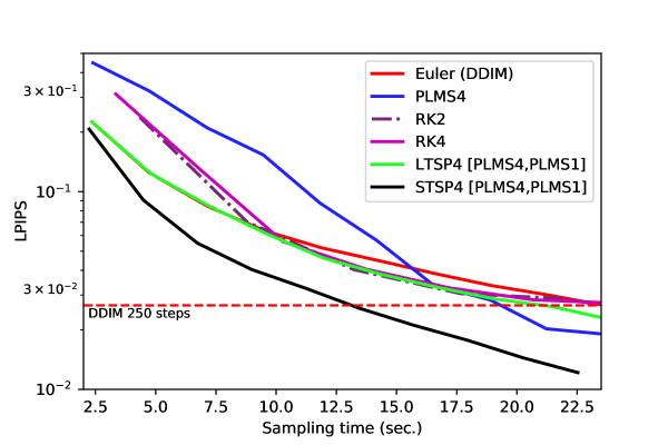
Figure 3: Comparison of different numerical methods for guided diffusion sampling.

	Sampling time within
	5 sec.	10 sec.	15 sec.	20 sec.
DDIM	0.116	0.062	0.043	0.033
PLMS4	0.278	0.141	0.057	0.026
RK2	0.193	0.059	0.036	0.028
RK4	0.216	0.054	0.039	0.028
LTSP4	0.121	0.058	0.037	0.028
STSP4	0.079	0.035	0.022	0.013

Figure 4: Average LPIPS when the sampling time is limited to be under 5 - 20 seconds.

In addition, we perform a quantitative evaluation for class-conditional generation by sampling 50,000 images based on uniformly chosen class conditions with a small number of sampling steps and evaluating the Fenchel Inception Distance (FID) Heusel et al. (2017) (lower is better) and the improved precision/recall Kynkäänniemi et al. (2019) (higher is better) against an ImageNet test set. Following (Dhariwal & Nichol, 2021), we use a 25-step DDIM as a baseline, which already produces visually reasonable results. As PLMS and LTSP require the same number of network evaluations as the DDIM, they are used also with 25 steps. For STSP with a longer network evaluation time, it is only allowed 20 steps, which is the highest number of steps such that its sampling time is within that of the baseline 25-step DDIM. Here LTSP2 and STSP2 are Lie-Trotter and Strang splitting methods with the combination [PLMS2, PLMS1]. In Table 1, we report the results of three different ImageNet resolutions and the average sampling time per image in seconds.

Our STSP4 performs best on all measurements except Recall on ImageNet512. On ImageNet512, PLMS4 has the highest Recall score but a poor FID of 16, indicating that the generated images have good distribution coverage but may poorly represent the real distribution. On ImageNet256, STSP4 can yield 4.49 FID in 20 steps, compared to 4.59 FID in 250 steps originally reported in the paper (Dhariwal & Nichol, 2021); our STSP4 is about 9.4$\times$ faster when tested on the same machine.

Method	Steps	Time	FID	Prec	Rec
ImageNet128
DDIM	25	0.55	6.69	0.78	0.49
PLMS2	25	0.57	5.71	0.80	0.51
PLMS4	25	0.57	4.97	0.80	0.53
LTSP2	25	0.55	5.14	0.81	0.51
LTSP4	25	0.55	3.85	0.81	0.54
STSP2	20	0.54	5.33	0.80	0.52
STSP4	20	0.54	3.78	0.81	0.54
[1.2pt/1.2pt] ADM-G	250	5.59*	2.97	0.78	0.59

Method	Steps	Time	FID	Prec	Rec
ImageNet256
DDIM	25	1.99	5.47	0.80	0.47
PLMS4	25	2.05	4.71	0.82	0.49
STSP4	20	1.95	4.49	0.83	0.50
[1.2pt/1.2pt] ADM-G	250	20.9*	4.59	0.82	0.50
ImageNet512
DDIM	25	5.56	9.07	0.81	0.42
PLMS4	25	5.78	16.00	0.75	0.51
STSP4	20	5.13	8.24	0.83	0.45
[1.2pt/1.2pt] ADM-G	250	56.2*	7.72	0.87	0.42

Table 1: Comparison of different numerical methods using a few steps on guided diffusion sampling. Our methods and the best scores are highlighted in bold. We provide the reported scores from Dhariwal & Nichol (2021) using 250 sampling steps, referred to as ADM-G in their paper. *ADM-G’s sampling times are measured using our machine.

4.3 Splitting methods in other tasks

Besides class-conditional generation, our approach can also accelerate any conditional image generation as long as the gradient of the conditional function can be defined. We test our approach on four tasks: text-to-image generation, image inpainting, colorization, and super-resolution.

Text-to-image generation: We use a pre-trained text-to-image Disco-Diffusion (Letts et al., 2021) based on Crowson (2021), which substitutes the classifier output with the dot product of the image and caption encodings from CLIP (Radford et al., 2021). For more related experiments on Stable-Diffusion (Rombach et al., 2022), please refer to Appendix L, M.

Image inpainting & colorization: For these two tasks, we follow the techniques proposed in Song et al. (2020b) and Chung et al. (2022a), which improves the conditional functions of both tasks with “manifold constraints.” We use the same diffusion model Dhariwal & Nichol (2021) trained on ImageNet as our earlier Experiments 4.1, 4.2.

Super-resolution: We follow the formulation from ILVR (Choi et al., 2021) combined with the manifold contraints Chung et al. (2022a), and also use our earlier ImageNet diffusion model.

“A beautiful painting of a singular lighthouse, shining its light across a tumultuous sea of blood, trending on artstation.”
“A beautiful painting of a starry night, over a sunflower sea, trending on artstation.”
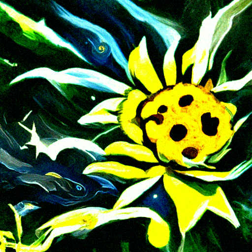
	Full DDIM	DDIM	PLMS4	LTSP4	STSP4
	(1,000 steps)	(45 steps)	(45 steps)	(45 steps)	(30 steps)
		(approximately using the same sampling time)

Figure 5: Text-to-image generation using different sampling methods.

Figure 5 compares our techniques, LTSP4 and STSP4, with the DDIM baseline and PLMS4 on text-to-image generation. Each result is produced using a fixed sampling time of about 26 seconds. STSP4, which uses 30 diffusion steps compared to 45 in the other methods, produces more realistic results with color contrast that is more similar to the full DDIM references’. Figure 6 shows that our STSP4 produces more convincing results than the DDIM baseline with fewer artifacts on the other three tasks while using the same 5 second sampling time. Implementation details, quantitative evaluations, and more results are in Appendix J, K.

	Original	Input	STSP4 (Ours)			DDIM
Inpainting
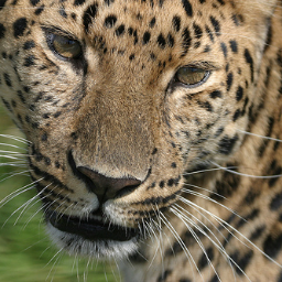
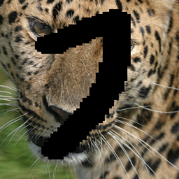
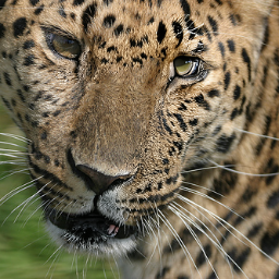
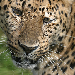
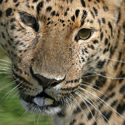
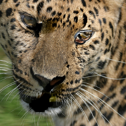
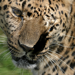
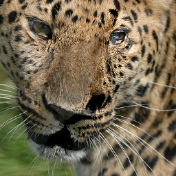
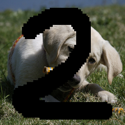
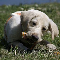
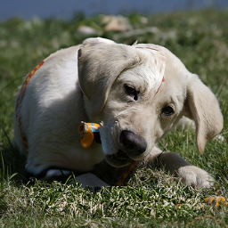
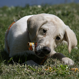
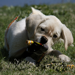
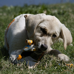
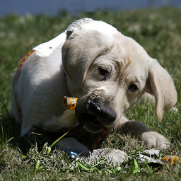
Colorization
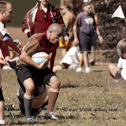
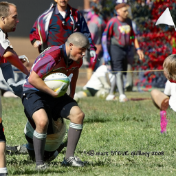
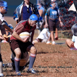
8xSuper-Resolution

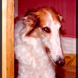
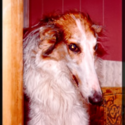
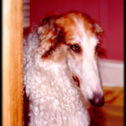
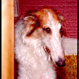
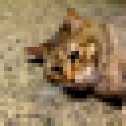
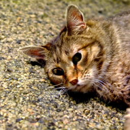
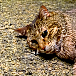
Figure 6: Guided-diffusion results of our STSP4 and DDIM on inpainting, colorization, and super-resolution. Both methods were limited to use approximately the same sampling time.

5 Discussion

Our findings show that when the sampling ODE consists of multiple terms from different networks, their numerical behaviors can be different and treating them separately can be more optimal. Another promising direction is to improve the behavior of the gradient of the conditional function / classifier itself and study whether related properties such as adversarial robustness or gradient smoothness can induce the desirable temporal smoothness in the sampling ODE. However, it is not yet clear what specific characteristics of the behavior play an important role. This challenge may be related to a condition called “stiffness” in solving ODEs Ernst & Gerhard (2010), which lacks a clear definition but describes the situation where explicit numerical methods, such as RK or PLMS, require a very small step size even in a region with smooth curvature.

As an alternative to the classifier-guided model, Ho & Salimans (2021) propose a classifier-free model that can perform conditional generation without a classifier while remaining a generative model. This model can utilize high-order methods as no classifier is involved, but it requires evaluating the classifier-free network twice per step, which is typically more expensive than evaluating a normal diffusion model and a classifier. It is important to note that our accelerating technique and classifier-free models are not mutually exclusive, and one can still apply a conditional function and our splitting technique to guide a classifier-free model in a direction it has not been trained for.

While our paper only focuses on ODEs derived from the deterministic sampling of DDIM, one can convert SDE-based diffusion models to ODEs (Karras et al., 2022) and still use our technique. More broadly, we can accelerate any diffusion model that can be expressed as a differential equation with a summation of two terms. When these terms behave differently, the benefit from splitting can be substantial. Nevertheless, our findings are based on common, existing models and $\sigma$ schedule from Dhariwal & Nichol (2021). Further investigation into the impact of the $\sigma$ schedule or different types and architectures of diffusion models is still required.

6 Conclusion

In this paper, we investigate the failure to accelerate guided diffusion sampling of classical high-order numerical methods and propose a solution based on splitting numerical methods. We found that the gradients of conditional functions are less suitable to classical high-order numerical methods and design a technique based on Strang splitting and a combination of forth- and first-order numerical methods. Our method achieves better LPIPS and FID scores than previous work given the same sampling time and is 32-58% faster than a 250-step DDIM baseline. Our technique can successfully accelerate a variety of tasks, such as text-to-image generation, inpainting, colorization, and super-resolution.

Appendix

Appendix A Implementation

Our implementation is available here. The implementation is based on Katherine Crowson’s guided-diffusion , which is inspired by OpenAI’s guided-diffusion. All of the pre-trained diffusion and classifier models are available here. For evaluation, we use OpenAI’s measurement implementation with their reference image batch, which can be found here.

Appendix B Improving PLMS

Initial points are required for using high-order PLMS. The fourth-order formulation, for example, requires three initial points. The original paper (Liu et al., 2022) employs the Runge-Kutta method to compute the initial points. However, Runge-Kutta’s method has high computational costs and is inconvenient to use when the number of steps is small. To reduce the computation costs, we compute the starting points of the higher-order PLMS using lower-order PLMS. Our PLMS can be summarized using Algorithm 3.

input: $\bar{x}_{n}$ (previous result), $\sigma_{n+1}$, $\sigma_{n}$,

$\{e_{i}\}_{i<n}$ (evaluation buffer), $r$ (method order) ;

 $e_{n}=\bar{\epsilon}_{\sigma}(\bar{x}_{n})$ ;

 $c=\min(r,n)$ ;

 if $c==1$ then

  $\hat{e}=e_{n}$ ;

 else if $c==2$ then

  $\hat{e}=(3e_{n}-e_{n-1})/2$ ;

 else if $c==3$ then

  $\hat{e}=(23e_{n}-16e_{n-1}+5e_{n-2})/12$ ;

 else

  $\hat{e}=(55e_{n}-59e_{n-1}+37e_{n-3}-9e_{n-4})/24$ ;

 Result: $\bar{x}_{n}+(\sigma_{n+1}-\sigma_{n})\hat{e}$

Algorithm 3 PLMS

In Algorithm 3, the PLMS formulation is obtained by assuming a constant $\Delta\sigma$ for each step. The results in our experiments and previous work (e.g., Liu et al. (2022); Zhang & Chen (2022)) are still reasonable when this assumption is not strictly satisfied, i.e., when $\Delta\sigma$ is not constant. Inspired by Zhang & Chen (2022), we also show how to derive another linear multi-step formulation for non-constant $\Delta\sigma$. Let us first define a dummy variable $\tau$ in which $\Delta\tau$ is a constant in each time step. To make it simple, let the value $\tau=0$ when $t=T$ and when $t=0$, $\tau=N$, the total number of steps. As a result, the discretization of $\tau$ can be defined by $\tau_{n}=n$ and $\Delta\tau=\tau_{n}-\tau_{n-1}=1$ is a constant. Next, we want to extrapolate the value of $\epsilon_{\theta}$ using a polynomial $P_{\epsilon}(\tau)$.

For example, the first order formulation can be produced by integrating a constant polynomial $P_{\epsilon}(\tau)=e_{n}$ :

$$\frac{d\bar{x}}{d\sigma}=\bar{\epsilon}(\bar{x})\approx P_{\epsilon}(\tau)=e_{n},$$

$$\int^{\bar{x}_{n+1}}_{\bar{x}_{n}}d\bar{x}= \int^{\sigma_{n+1}}_{\sigma_{n}}e_{n}\>d\sigma,$$

$$\bar{x}_{n+1}-\bar{x}_{n}= e_{n}\Delta\sigma$$

which leads us to Euler’s formulation. Rather than using Lagrange’s polynomial like Zhang & Chen (2022), we use Newton’s polynomial, which gives a nicer final formulation. However, both are the same polynomial but have different expressions. For the 2^nd order formulation, we interpolate between $(\tau_{n},e_{n})$ and $(\tau_{n-1},e_{n-1})$ using a Newton’s polynomial $P_{\epsilon}(\tau)=e_{n}+(e_{n}-e_{n-1})(\tau-\tau_{n})$.

$$\int^{\bar{x}_{n+1}}_{\bar{x}_{n}}d\bar{x}=\int^{\sigma_{n+1}}_{\sigma_{n}}e_{n}+(e_{n}-e_{n-1})(\tau-\tau_{n})d\sigma.$$

Every term is the same as in the 1^st order formulation, except for one term that is $\int^{\sigma_{n+1}}_{\sigma_{n}}(\tau-\tau_{n})d\sigma$. Let us use separable integration to approximate this term.

$$\int^{\sigma_{n+1}}_{\sigma_{n}}(\tau-\tau_{n})d\sigma=\int^{\tau_{n+1}}_{\tau_{n}}(\tau-\tau_{n})\frac{d\sigma}{d\tau}d\tau\approx\int^{\tau_{n+1}}_{\tau_{n}}(\tau-\tau_{n})d\tau\int^{\tau_{n+1}}_{\tau_{n}}\frac{d\sigma}{d\tau}d\tau=\frac{\Delta\sigma}{2}$$

The result is $\bar{x}_{n+1}-\bar{x}_{n}=e_{n}\Delta\sigma+(e_{n}-e_{n+1})\frac{\Delta\sigma}{2}$, which is the PLMS2 formulation. To compute this term more precisely, we need to know the derivation $d\sigma/d\tau$. For this example, let us define $\sigma$ by

$$\sigma(\tau)=\exp\left(\ln{\sigma_{\text{max}}}+\frac{\tau}{N}(\ln{\sigma_{\text{min}}}-\ln{\sigma_{\text{max}}})\right)=\exp(a+\tau b),$$ (16)

where $a=\ln{\sigma_{\text{max}}}$ and $b=(\ln{\sigma_{\text{min}}}-\ln{\sigma_{\text{max}}})/N$. Now, we have

$$\int^{\tau_{n+1}}_{\tau_{n}}(\tau-\tau_{n})\frac{d\sigma}{d\tau}d\tau=\Delta\sigma\left(\frac{\exp(b)}{\exp(b)-1}-\frac{1}{b}\right).$$

Consider $\frac{\exp(b)}{\exp(b)-1}-\frac{1}{b}$ when limit $N\rightarrow\infty$ (or $b\rightarrow 0$), this term is equal to $\frac{1}{2}$, which turns the formulation back to PLMS2. When we set $N=30$ (or $b=-0.33$), the term $\frac{\exp(b)}{\exp(b)-1}-\frac{1}{b}=0.4723$, which is also close to $\frac{1}{2}$ in PLMS2 formulation.

We can continue using higher-order Newton’s polynomials to obtain higher-order formulations. We call this method GLMS (Generalized Linear Multi-Step) and summarize it with Algorithm 4. In our comparison in Figure 7, both PLMS and GLMS produce comparable results. In the fourth order, GLMS4 performs slightly better than PLMS4. However, the GLMS formulation is dependent on the $\sigma$ schedule, and the formulation must be revised if the $\sigma$ schedule changes. As a result, we decided to use PLMS as part of our main algorithm for more flexibility.

input: $\bar{x}_{n}$ (previous result), $\sigma_{n+1}$, $\sigma_{n}$, $\{e_{i}\}_{i<n}$ (evaluation buffer), $r$ (method order) ;

 $b=\ln(\sigma_{n+1})-\ln(\sigma_{n})$  $e_{n}=\bar{\epsilon}_{\sigma}(\bar{x}_{n})$ ;  $\{e_{i}\}$.append($e_{n}$) ;  $c=\min(r,n)$ ;

 if $c\geq 1$ then

  $\hat{e}=e_{n}$ ;

 if $c\geq 2$ then

  $\hat{e}=\hat{e}+(e_{n}-e_{n-1})\left(\frac{\exp(b)}{\exp(b)-1}-\frac{1}{b}\right)$ ;

 if $c\geq 3$ then

  $\hat{e}=\hat{e}+(e_{n}-2e_{n-1}+e_{n-2})\left(\frac{\exp(b)}{\exp(b)-1}(2-\frac{2}{b})-\frac{1}{b}+\frac{2}{b^{2}}\right)$ ;

 if $c\geq 4$ then

  $\hat{e}=\hat{e}+(e_{n}-3e_{n-1}+3e_{n-2}-e_{n-3})\left(\frac{\exp(b)}{\exp(b)-1}(6-\frac{9}{b}+\frac{6}{b^{2}})-\frac{2}{b}+\frac{6}{b^{2}}-\frac{6}{b^{3}}\right)$ ;

 Result: $\bar{x}_{n}+(\sigma_{n+1}-\sigma_{n})\hat{e}$

Algorithm 4 GLMS

Appendix C Numerical Methods for Unguided Diffusion

This experiment evaluates the numerical methods used in our paper on unguided sampling to see whether they may behave differently. We perform a similar experiment as in Section 4.1, 4.2 except on an unguided, unconditional diffusion model and use samples from 1,000-step DDIM as reference images. For each method, we use the same initial noise maps as the DDIM and evaluate the image similarity between its generated images and the reference images based on LPIPS. Figure 7 reports LPIPS vs sampling time for ImageNet128 using the $\sigma$ schedule in Equation 16.

We found that RK2 and RK4 perform better than DDIM, but in our main papers these methods perform worse than DDIM when used on the split sub-problems for guided sampling. Linear multi-step methods continue to be the best performers. The graph also shows that higher order is generally better, especially when the number of steps is large.

Appendix D Comparing PLMS and DEIS

In Tables 2 and 3, we compare the coefficients $e_{n},e_{n-1},e_{n-2}$, and $e_{n-3}$ of PLMS in Algorithm 3 and the original implementation DEIS Zhang & Chen (2022) using the default linear schedule and 10 sampling steps. This shows that DEIS and PLMS are two similar methods. DEIS is analogous to PLMS with non-fixed coefficients. The coefficients can change depending on the number of steps and the noise schedule. However, the coefficients from both methods are close, and as previously stated, the DEIS coefficients will converge to the PLMS coefficients. Since DEIS’s implementation relies heavily on the noise schedule, if the schedule changes, we must re-implement the method. For these reasons, we prefer PLMS over DEIS for practical purposes.

coefficient of n^th step $e_{n}$ $e_{n-1}$ $e_{n-2}$ $e_{n-3}$ 1 1.0 0. 0. 0. 2 1.5 -0.5 0. 0. 3 1.5 -0.5 0. 0. 4 1.5 -0.5 0. 0. 5 1.5 -0.5 0. 0. 6 1.5 -0.5 0. 0. 7 1.5 -0.5 0. 0. 8 1.5 -0.5 0. 0. 9 1.5 -0.5 0. 0. 10 1.5 -0.5 0. 0. (a) PLMS

coefficient of n^th step $e_{n}$ $e_{n-1}$ $e_{n-2}$ $e_{n-3}$ 1 1.00 0. 0. 0. 2 1.42 -0.42 0. 0. 3 1.43 -0.43 0. 0. 4 1.43 -0.43 0. 0. 5 1.44 -0.44 0. 0. 6 1.45 -0.45 0. 0. 7 1.46 -0.46 0. 0. 8 1.47 -0.47 0. 0. 9 1.48 -0.48 0. 0. 10 1.50 -0.50 0. 0. (b) DEIS

Table 2: Comparison of DEIS and PLMS on second order

coefficient of n^th step $e_{n}$ $e_{n-1}$ $e_{n-2}$ $e_{n-3}$ 1 1.0 0. 0. 0. 2 1.5 -0.5 0. 0. 3 1.92 -1.33 0.41 0. 4 2.29 -2.46 1.54 -0.38 5 2.29 -2.46 1.54 -0.38 6 2.29 -2.46 1.54 -0.38 7 2.29 -2.46 1.54 -0.38 8 2.29 -2.46 1.54 -0.38 9 2.29 -2.46 1.54 -0.38 10 2.29 -2.46 1.54 -0.38 (a) PLMS

coefficient of n^th step $e_{n}$ $e_{n-1}$ $e_{n-2}$ $e_{n-3}$ 1 1.0 0. 0. 0. 2 1.42 -0.42 0. 0. 3 1.77 -1.12 0.34 0. 4 2.09 -2.07 1.28 -0.34 5 2.11 -2.11 1.31 -0.32 6 2.14 -2.16 1.35 -0.33 7 2.16 -2.22 1.38 -0.34 8 2.20 -2.28 1.42 -0.35 9 2.23 -2.35 1.47 -0.35 10 2.23 -2.28 1.55 -0.38 (b) DEIS

Table 3: Comparison of DEIS and PLMS on forth order

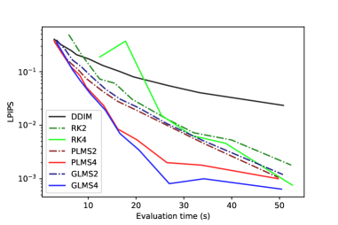
Figure 7: Comparison of different numerical methods on an unguided diffusion model. Using samples from a 1000-step DDIM as reference solutions, we measure average LPIPS scores and plot them against the average sampling time.

Appendix E LPIPS vs. the number of sampling step

We report additional LPIPS results of the experiment in Section 4.1 but with respect to the number of sampling steps. The result shows that methods in the RK family can outperform other methods given the same number of sampling steps. However, once taken into account the slower evaluation time per step, these methods are overall slower to reach the same level of LPIPS of other methods.

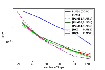
(a) Vary method for diffusion subproblem

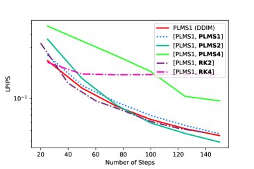
(b) Vary method for condition subproblem

Figure 8: In addition to Figure 4.1, we plot LPIPS against their sampling steps. RK family can outperform other methods in many situations. However, methods in RK family took a longer time per diffusion step.

Appendix F More Statistics for Experiement 4.2

We report the mean and standard deviation of each LPIPS score of the experiment in Section 4.2 in Table 4. In Table 5, we report the $p$-value for the null hypothesis that our STSP4 performs worse than other methods.

	Sampling time within
	5 sec.	10 sec.	15 sec.	20 sec.
DDIM	0.111 $\pm$ .078	0.062 $\pm$ .065	0.042 $\pm$ .056	0.031 $\pm$ .048
PLMS4	0.240 $\pm$ .131	0.085 $\pm$ .112	0.039 $\pm$ .072	0.018 $\pm$ .040
RK2	0.152 $\pm$ .090	0.048 $\pm$ .051	0.030 $\pm$ .037	0.026 $\pm$ .037
RK4	0.190 $\pm$ .106	0.044 $\pm$ .022	0.033 $\pm$ .038	0.019 $\pm$ .032
LTSP4	0.111 $\pm$ .092	0.056 $\pm$ .060	0.040 $\pm$ .054	0.028 $\pm$ .046
STSP4	0.072 $\pm$ .065	0.033 $\pm$ .044	0.018 $\pm$ .028	0.012 $\pm$ .022

Table 4: Our STSP4 has low average LPIPS scores and low standard deviations of LPIPS (N=120 samples).

	Sampling time within
	5 sec.	10 sec.	15 sec.	20 sec.
DDIM	$9.1\times 10^{-11}$	$9.0\times 10^{-10}$	$7.1\times 10^{-9}$	$9.2\times 10^{-8}$
PLMS4	$3.3\times 10^{-41}$	$2.1\times 10^{-13}$	$8.1\times 10^{-4}$	$3.7\times 10^{-2}$
RK2	$1.2\times 10^{-30}$	$6.4\times 10^{-5}$	$6.1\times 10^{-5}$	$2.5\times 10^{-7}$
RK4	$5.0\times 10^{-31}$	$6.2\times 10^{-3}$	$6.1\times 10^{-5}$	$1.6\times 10^{-3}$
LTSP4	$5.6\times 10^{-11}$	$9.1\times 10^{-11}$	$2.8\times 10^{-10}$	$1.7\times 10^{-7}$

Table 5: $p$-value for STSP4 has lower average LPIPS scores compare to other methods at approximately the same sampling time.

Appendix G STSP4 vs. More Numerical Methods Combination

We extend the experiment from Section 4.2 and compare our STSP4 and DDIM baselines with more numerical method combinations. Here we report LPIPS vs sampling time in Figure 9. The results show that Strang splitting method with [PLMS4, PLMS1] (our STSP4) is still the best combination, similar to the finding in Section 4.2.

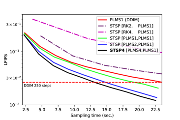
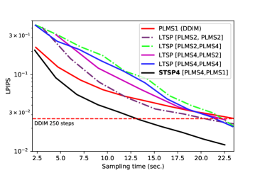
Figure 9: We compare using Strang splitting with different numerical methods on the diffusion subproblem.

Appendix H Comparison with DEIS and DPM-solver

We compare our splitting method to DPM-solver Lu et al. (2022) and DEIS Zhang & Chen (2022). Since both methods have different implementation details, such as using different noise schedules, which affect the ODE solution, these methods do not converge to the same exact solution. Thus, it is not sensible to directly compare them, and we instead implement our method in their official implementations of DPM-solver Lu et al. (2022) and DEIS Zhang & Chen (2022). We then compare the results with LPIPS on classifier-guided diffusion pretrained on ImageNet256 similar to Table 4 in Section 4. The results are shown in Table 6 and 7. Our splitting methods can perform better than both DPM-solver Lu et al. (2022) and DEIS Zhang & Chen (2022).

	Sampling time within
	5 sec.	10 sec.	15 sec.	20 sec.
DPM-Solver-1 (DDIM)	0.333	0.125	0.080	0.045
DPM-Solver-2	0.565	0.188	0.078	0.045
DPM-Solver-3	0.540	0.233	0.087	0.043
LTSP4	0.185	0.105	0.071	0.048
STSP4	0.169	0.062	0.061	0.037

Table 6: The comparison with DPM-solver Lu et al. (2022). Average LPIPS when the sampling time is limited to be under 5-20 seconds.

	Sampling time within
	3 sec.	6 sec.	9 sec.	12 sec.
0-DEIS (DDIM)	0.333	0.125	0.080	0.045
1-DEIS	0.466	0.193	0.092	0.044
3-DEIS	0.625	0.511	0.433	0.345
LTSP4	0.321	0.120	0.080	0.048
STSP4	0.212	0.080	0.046	0.031

Table 7: Comparison with DEIS Zhang & Chen (2022). We report the average LPIPS scores when the sampling time is limited to be under 3-12 seconds.

Appendix I Experiment on FID vs. Sampling Time

In this section, we demonstrate how splitting methods can accelerate guided diffusion sampling using FID scores. We vary the number of sampling steps, generate 20k samples, and compare the FID of the splitting methods (LTSP4 and STSP4) to many non-splitting methods, including DDIM, PLMS4, RK2, and RK4. Figure 10 shows a comparison of FID vs. sampling time for each method. This experiment uses a classifier-guided diffusion model that was pretrained on the ImageNet128 dataset by Dhariwal & Nichol (2021). Our method can generate good sample quality, especially when the average sampling is limited to under 0.3 seconds (or about 50 steps of DDIM for 128$\times$128 resolution), while other methods show large FID scores at lower sampling steps or require more time to generate similarly high-quality samples.

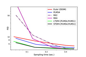
Figure 10: FID vs. Sampling time measured on ImageNet128

Appendix J Text-guided image generation

For text-to-image generation or text-guided image generation, our implementation is based on Disco-Diffusion v3.1, which also relies on Crowson (2021). We use v3.1 that does not contain unrelated features; however, our method can be applied to any of the versions. We use the fine-tuned 512x512 diffusion model from Katherine Crowson and use pre-trained OpenAI’s CLIP models including RN50, ViTB32, and ViTB16. For other model and conditional function configurations, we use Disco-Diffusion v3.1’s default settings.

Appendix K Controllable generation

We provide implementation details of our sampling algorithm for other conditional generation tasks.

Image inpainting: Given a target masked image, $y_{0}$, and a mask $P$ which is a matrix of $0,1$ values, we want to sample $x_{0}$ so that $y_{0}=Px_{0}$. The key concept from Song et al. (2020b) is to use reverse diffusion in the unmasked area and forward diffusion in the masked area through an additional step called the impose step. Let $x^{\prime}_{t-1}$ be an unconditional diffusion sample from $x_{t}$ and $y_{t-1}$ be a forward diffusion sample from $y_{0}$. The impose step can be summarized as follows:

$$x_{t-1}=(I-P^{T}P)x^{\prime}_{t-1}+P^{T}y_{t-1}.$$ (17)

To sample a corrupted target image $y_{t-1}$, we use the sampling formulation from Song et al. (2020a) to sample from $y_{0}$ by

$$y_{t}\sim\mathcal{N}(\sqrt{\bar{\alpha}_{t}}y_{0}+\sqrt{1-\bar{\alpha}_{t}-\eta^{2}_{t}}\epsilon_{\theta}(x_{t},t),\eta^{2}_{t}I)$$ (18)

where $\eta_{t}=\sqrt{(1-\bar{\alpha}_{t-1})/(1-\bar{\alpha}_{t}})\sqrt{1-\bar{\alpha}_{t}/\bar{\alpha}_{t-1}}$. This formulation works more effectively with numerical methods than the original sampling formulation from Song et al. (2020b), which is $y_{t}\sim\mathcal{N}(\sqrt{\bar{\alpha}_{t}}y_{0},(1-\bar{\alpha}_{t})I)$.

Rather than sampling $x^{\prime}_{t-1}$ unconditionally, we follow Chung et al. (2022a) and use guided diffusion sampling with the conditional function defined by:

$$f(x_{t})=\frac{1}{2\gamma}||y_{0}-P\hat{x}_{0}(x_{t})||^{2}_{2},\quad\hat{x}_{0}(x_{t})=\frac{x_{t}-\sqrt{1-\bar{\alpha}_{t}}\epsilon_{\theta}(x_{t},t)}{\sqrt{\bar{\alpha}_{t}}},$$ (19)

where $\gamma$ is a control parameter. Since directly computing $\epsilon_{\theta}(x_{t},t)$ with the diffusion network in Equation 18 and 19 is time consuming, we use a secondary-model method from Katherine Crowson to speed it up.

Image colorization: The idea behind colorization is very similar to inpainting. We convert images from the RGB format to the HSV format, with the grayscale value in the first channel, using an orthogonal matrix:

$$C=\begin{bmatrix}0.577&-0.816&0\\ 0.577&0.408&0.707\\ 0.577&0.408&-0.707\\ \end{bmatrix}.$$

To mask out other channels and keep only the first grayscale channel, we define the mask matrix $P$ as 1 in the grayscale channel and 0 in the other two channels. The impose step and conditional function can be defined as

$$x_{t-1}=(I-C^{T}P^{T}PC)x^{\prime}_{t-1}+C^{T}P^{T}PCy_{t-1},\quad f(x_{t})=\frac{1}{2\gamma}||y_{0}-PC\hat{x}_{0}(x_{t})||^{2}.$$

Image super-resolution: Let us denote $D$ as a down-sampling matrix. The impose step and conditional function is given by

$$x_{t-1}=(I-D^{T}D)x^{\prime}_{t-1}+D^{T}y_{t-1},\quad f(x_{t})=\frac{1}{2\gamma}||y_{0}-D\hat{x}_{0}(x_{t})||^{2}.$$

In our implementation, we replace the $D$ and $D^{T}$ operations with the ILVR (Choi et al., 2021) down-sampling and up-sampling functions.

Figure 11, 12, and 13 show additional qualitative results on the three tasks. We evaluate LPIPS and PSNR between the generated images and their original images for the three tasks in Table 8. Our test set consists of 200 input images, and each test image will be used to produce 6 samples for each task for the evaluation.

Note that LPIPS and PSNR are not the ideal measurements for this evaluation, but they are a de facto standard for benchmarking. Our goal here is to demonstrate how our technique can generalize to other conditional generation tasks. Non-diffusion techniques can not be compared the acceleration effect with ours since they are based on completely different things. Some comparison of the diffusion technique to other techniques can also be found in Chung et al. (2022a). To achieve state-of-the-art performance on these tasks in terms of quality and speed, other recent techniques may be more suitable, such as improved initialization (Chung et al., 2022b) and forward-backward repetition (Meng et al., 2021). However, our contributions are orthogonal to these investigations.

	Inpainting		Colorization		Super-resolution
Methods	LPIPS	PSNR	LPIPS	PSNR	LPIPS	PSNR
DDIM	0.17	19.52	0.28	20.40	0.46	17.88
PLMS4	0.25	15.01	0.47	13.50	0.73	7.85
LTSP4	0.17	19.61	0.31	19.40	0.51	16.07
STSP4	0.16	20.03	0.26	21.27	0.42	19.34

Table 8: Average LPIPS and PSNR scores from different methods on three different tasks.

Original	Input		STSP4			DDIM

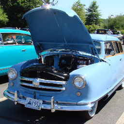
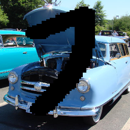
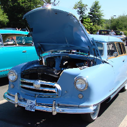
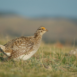
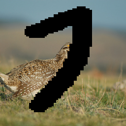
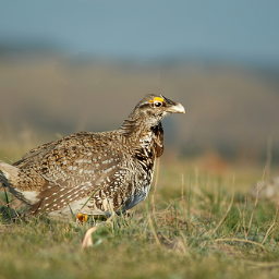
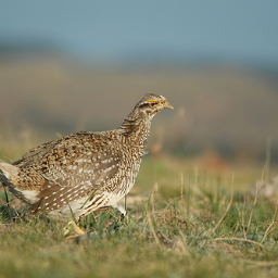
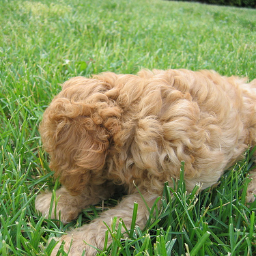
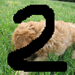
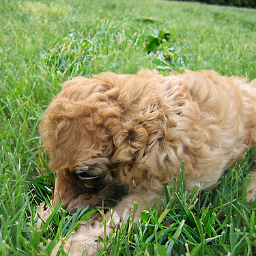
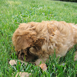
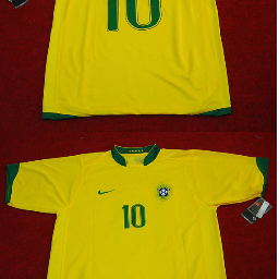
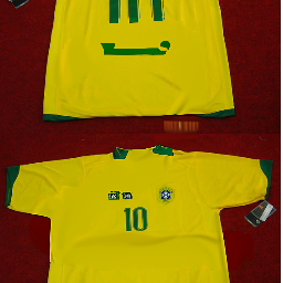
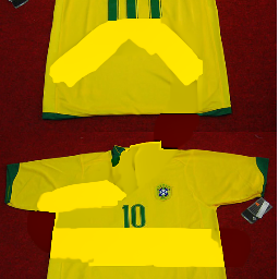
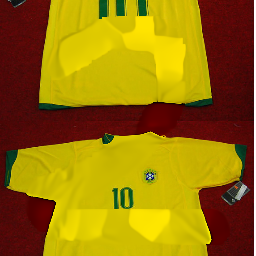
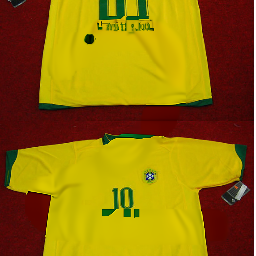
Figure 11: Additional inpainting results on ImageNet256. We show three different results generated by each method for each input. All results are generated using the same 5 second sampling time.

Original	Input		STSP4			DDIM

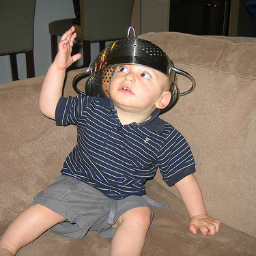
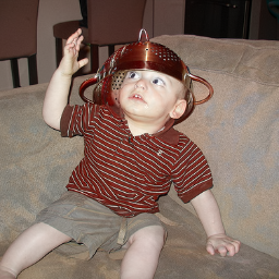
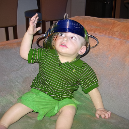
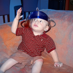
Figure 12: Additional colorization results on ImageNet256. We show three different results generated by each method for each input. All results are generated using the same 5 second sampling time.

Original	Input		STSP4			DDIM

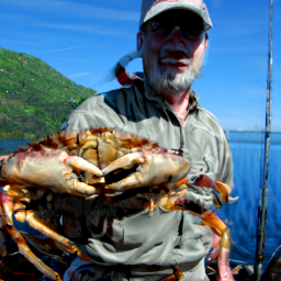
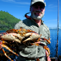
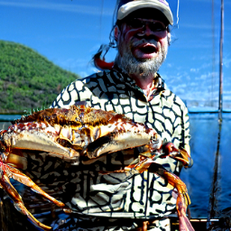
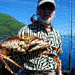
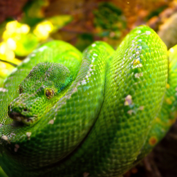
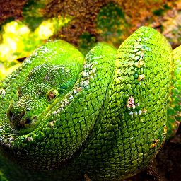
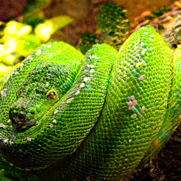
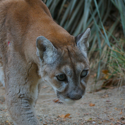
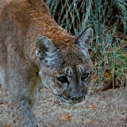
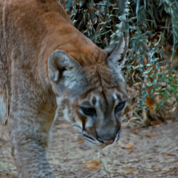
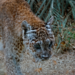
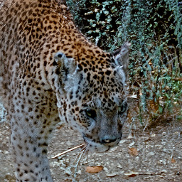
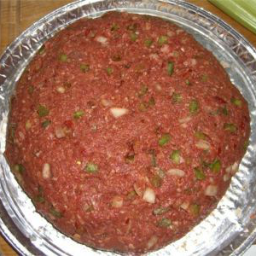
Figure 13: Additional 8x super-resolution results on ImageNet256. We show three different results generated by each method for each input. All results are generated using the same 5 second sampling time.

Appendix L Dreambooth Stable Diffusion

Dreambooth (Ruiz et al., 2022) is a technique for fine-tuning a pretrained text-to-image diffusion model on a given set of images. We discover that, similar to guided diffusion models, Dreambooth on Stable Diffusion (a pretrained text-guided latent-space diffusion) sometimes cannot be used with high-order methods but can be accelerated by our proposed method. This example demonstrates that our splitting method is effective not only on classifier-guided models but also classifier-free diffusion models.

The guided ODE of a classifier-free model is given by

$$\frac{d\bar{x}}{d\sigma}=\bar{\epsilon}_{\sigma}(\bar{x}|\phi)+s(\bar{\epsilon}_{\sigma}(\bar{x}|c)-\bar{\epsilon}_{\sigma}(\bar{x}|\phi)),$$ (20)

where $c$ is the input prompt, $\bar{\epsilon}_{\sigma}(\bar{x}|c)$ is the network output conditioned on the input prompt, and $\bar{\epsilon}_{\sigma}(\bar{x}|\phi)$ is the network output conditioned on a null label $\phi$. We can split the guided ODE into two subproblems as follows:

$$\frac{dy}{d\sigma}=\bar{\epsilon}_{\sigma}(y|\phi),\quad\frac{dz}{d\sigma}=s(\bar{\epsilon}_{\sigma}(z|c)-\bar{\epsilon}_{\sigma}(z|\phi)).$$ (21)

We test on “mo-di-diffusion”, a Dreambooth Stable Diffusion model that was fine-tuned on a dataset of screenshots from Disney studio. We use the prompt “ a girl face in modern Disney style.” The result is shown in Figure 14. However, we believe that Dreambooth diffusion models may have different problems from classifier-guided diffusion models and deserve their own in-depth study.

Number of steps	20         40        80       160
PLMS4 (Liu et al., 2022)
LTSP4 (Ours)
STSP4 (Ours)

Figure 14: Generated samples from a text-guided Stable Diffusion model fine-tuned on a dataset of screenshots from Disney studio using 20-160 sampling steps. Our splitting technique produces high-quality results in fewer sampling steps. prompt: “a girl face in modern Disney style”

Appendix M CLIP-Guided Stable Diffusion

UPainting (Li et al., 2022) suggest that text-to-image Stable Diffusion quality can be improve using gradient from CLIP model. This is an example of combining classifier-free and gradient-guided technique to obtain better result. As we have demonstrated in our paper, adding a gradient term to the diffusion model can cause high-order methods fail to accelerate sampling. The guided ODE 8 can be modified as follows:

$$\frac{d\bar{x}}{d\sigma}=\bar{\epsilon}_{\sigma}(\bar{x}|\phi)+s(\bar{\epsilon}_{\sigma}(\bar{x}|c)-\bar{\epsilon}_{\sigma}(\bar{x}|\phi))-\lambda\nabla_{\bar{x}}(f_{\text{img}}(\bar{x})\cdot f_{\text{txt}}(a)),$$ (22)

where $f_{\text{img}}(\bar{x})$ is CLIP’s image encoder output and $f_{\text{txt}}(a)$ is the output of CLIP’s text encoder. We can apply our method by splitting the Equation 22 into two subproblems by

$$\frac{dy}{d\sigma}=\bar{\epsilon}_{\sigma}(y|\phi)+s(\bar{\epsilon}_{\sigma}(y|c)-\bar{\epsilon}_{\sigma}(y|\phi)),\quad\frac{dz}{d\sigma}=-\lambda\nabla_{z}(f_{\text{img}}(z)\cdot f_{\text{txt}}(a)).$$ (23)

We show sample images using different numerical methods in Figure 15. Our method produces high-quality results in fewer sampling steps.

Stable Diffusion’s prompt: “a ball” CLIP’s prompt: “a metal sphere”
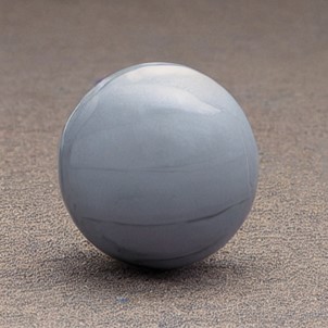
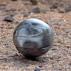
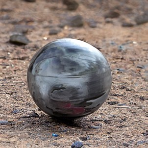
Stable Diffusion’s prompt: “a ball” CLIP’s prompt: “a red apple”
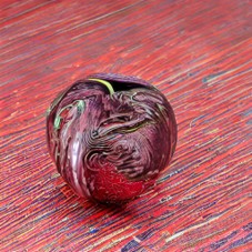
	PLMS4	LTSP4	STSP4
	(Liu et al., 2022)	(Ours)	(Ours)
	(100 steps)	(100 steps)	(55 steps)

Figure 15: Text-to-image generation using CLIP-guided Stable Diffusion from different high-order sampling methods with approximately the same sampling time.

Appendix N Convergence Orders of Methods

In this section, we show the convergence order of Lie-Trotter and Strang splitting methods. Suppose the differential equation we want to solve is defined by

$$\frac{dx}{dt}=f_{0}(x)=f_{1}(x)+f_{2}(x),$$ (24)

where $f_{1},f_{2}$ are assumed to be differentiable. We define $\Phi_{\Delta t,f_{i}}$ as a mapping solution of an ODE $\frac{dx}{dt}=f_{i}(x,t)$ in an interval $[t_{0},t_{0}+\Delta t]$. Noting that $\Phi_{0,f_{i}}(x)=x$ and $\frac{d}{dt}\Phi_{\Delta t,f_{i}}(x)=f_{i}(x)$.

By perform a Taylor expansion, we have

$$\Phi_{\Delta t,f_{i}}(x)=x+\Delta tf_{i}(x)+\frac{(\Delta t)^{2}}{2}f^{\prime}_{i}(x)f_{i}(x)+\mathcal{O}(\Delta t^{3}).$$ (25)

Lie-Trotter splitting

A single step of the Lie-Trotter splitting method can be expressed as $\Phi_{\Delta t,f_{2}}(\Phi_{\Delta t,f_{1}}(x))$. Applying the expansion of Equation 25 to this formulation gives:

$$\Phi_{\Delta t,f_{2}}(\Phi_{\Delta t,f_{1}}(x)) =[x+\Delta tf_{1}(x)+\mathcal{O}(\Delta t^{2})]+\Delta tf_{2}[x+\Delta tf_{1}(x)+\mathcal{O}(\Delta t^{2})]+\mathcal{O}(\Delta t^{2})$$

$$=x+\Delta tf_{1}(x)+\Delta tf_{2}(x)+\mathcal{O}(\Delta t^{2})$$

$$=\Phi_{\Delta t,f_{0}}(x)+\mathcal{O}(\Delta t^{2}).$$ (26)

Hence, the Lie-Trotter splitting method is of first-order.

Strang splitting

Consider a single step of the Strang splitting, which is $\Phi_{\Delta t/2,f_{2}}(\Phi_{\Delta t,f_{1}}(\Phi_{\Delta t/2,f_{2}}(x)))$. To show the second-order accuracy of the Strange splitting, we first expand the two inner operators.

$$\Phi_{\Delta t,f_{1}}(\Phi_{\Delta t/2,f_{2}}(x)) =[x+\frac{\Delta t}{2}f_{2}(x)+\frac{(\Delta t)^{2}}{2^{2}2!}f^{\prime}_{2}(x)f_{2}(x)+\mathcal{O}(\Delta t^{3})]$$

$$+(\Delta t)f_{1}[x+\frac{\Delta t}{2}f_{2}(x)+\mathcal{O}(\Delta t^{2})]$$

$$+\frac{(\Delta t)^{2}}{2}f^{\prime}_{1}[x+\mathcal{O}(\Delta t)]f_{1}[x+\mathcal{O}(\Delta t)]+\mathcal{O}(\Delta t^{3})$$ (27)

$$=x+\frac{\Delta t}{2}f_{2}(x)+\frac{(\Delta t)^{2}}{2^{2}2!}f^{\prime}_{2}(x)f_{2}(x)$$

$$+(\Delta t)f_{1}(x)+\frac{(\Delta t)^{2}}{2}f^{\prime}_{1}(x)f_{2}(x)$$

$$+\frac{(\Delta t)^{2}}{2}f^{\prime}_{1}(x)f_{1}(x)+\mathcal{O}(\Delta t^{3})$$ (28)

Consequently,

$$\Phi_{\frac{\Delta t}{2},f_{2}}(\Phi_{\Delta t,f_{1}}(\Phi_{\frac{\Delta t}{2},f_{2}}(x))) =x+(\Delta t)f_{1}(x)+\frac{\Delta t}{2}f_{2}(x)$$

$$+\frac{(\Delta t)^{2}}{2^{2}2!}f^{\prime}_{2}(x)f_{2}(x)+\frac{(\Delta t)^{2}}{2}f^{\prime}_{1}(x)f_{2}(x)+\frac{(\Delta t)^{2}}{2!}f^{\prime}_{1}(x)f_{1}(x)$$

$$+\frac{\Delta t}{2}f_{2}[x+(\Delta t)f_{1}(x)+\frac{\Delta t}{2}f_{2}(x)+\mathcal{O}(\Delta t^{2})]$$

$$+\frac{(\Delta t)^{2}}{2^{2}2!}f^{\prime}_{2}[x+\mathcal{O}(\Delta t)]f_{2}[x+\mathcal{O}(\Delta t)]+\mathcal{O}(\Delta t^{3})$$ (29)

$$\Phi_{\frac{\Delta t}{2},f_{2}}(\Phi_{\Delta t,f_{1}}(\Phi_{\frac{\Delta t}{2},f_{2}}(x))) =x+(\Delta t)f_{1}(x)+(\Delta t)f_{2}(x)$$

$$+\frac{(\Delta t)^{2}}{2!}[f^{\prime}_{1}(x)f_{1}(x)+f^{\prime}_{1}(x)f_{2}(x)+f^{\prime}_{2}(x)f_{1}(x)+f^{\prime}_{2}(x)f_{2}(x)]$$

$$+\mathcal{O}(\Delta t^{3})$$ (30)

$$=x+(\Delta t)f_{0}(x)+\frac{(\Delta t)^{2}}{2!}f^{\prime}_{0}(x)f_{0}(x)+\mathcal{O}(\Delta t^{3})$$ (31)

$$=\Phi_{\Delta t,f_{0}}(x)+\mathcal{O}(\Delta t^{3})$$ (32)

Therefore, the Strang splitting method’s convergence rate is of second-order.

Appendix O Toy Example

In this section, we create a toy example to demonstrate how high-order numerical methods can become unstable on a certain class of ODE problems (Stiff equation) despite involving no neural networks. Let us define the following ODE:

$$\frac{dx}{dt}=\epsilon(x)+s\cdot g(x),\qquad x(0)=\begin{bmatrix}1\\ 0\end{bmatrix},$$ (33)

where $s$ is a scaling parameter and

$$\epsilon\left(\begin{bmatrix}x_{1}\\ x_{2}\end{bmatrix}\right)=\begin{bmatrix}0&1\\ -1&-2\end{bmatrix}\begin{bmatrix}x_{1}\\ x_{2}\end{bmatrix},\quad g\left(\begin{bmatrix}x_{1}\\ x_{2}\end{bmatrix}\right)=\begin{bmatrix}0&0\\ -1&-1\end{bmatrix}\begin{bmatrix}x_{1}\\ x_{2}\end{bmatrix}.$$ (34)

Figure 16 depicts solution trajectories of various numerical methods We can observe that the PLMS4’s trajectory can run far from the exact solution than the Euler’s method or the splitting methods, LSTP4 and STSP4. The exact solution of Equation 33 is

$$x(t)=\frac{1}{s}\begin{bmatrix}-1\\ s+1\end{bmatrix}e^{-(s+1)t}+\frac{1}{s}\begin{bmatrix}s+1\\ -s-1\end{bmatrix}e^{-t}.$$ (35)

When $s$ increases, the term $e^{-(s+1)t}$ decays to zero more rapidly than the term $e^{-t}$. When the two terms behave differently, classical high-order numerical methods tend to perform poorly unless they employ a very small step size.

$s=3$
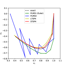
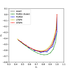
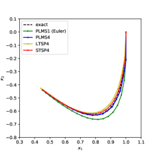
$s=5$
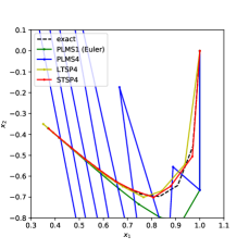
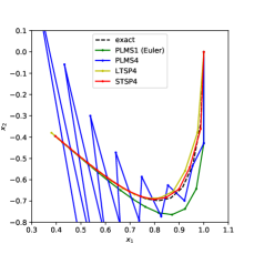
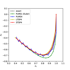
	10 steps	15 steps	20 steps

Figure 16: Solution trajectories of different numerical methods on a toy ODE problem using different numbers of steps. Non-splitting methods especially PLMS4 are more likely to fail to converge to the exact solution when the number of steps is reduced.

Appendix P Stability Analysis

In this section, we further analyze numerical solutions using stability analysis. We compute the lowest number of steps before the numerical solution is guaranteed to diverge by theory and visualize the solution trajectories using different numbers of steps to empirically support the theory. We only focus on Euler and other second-order numerical methods in this part.

One way to analyze numerical methods that solve Equation 33 is to evaluate them with a test equation that leads to the solution $y(t)=e^{-(s+1)t}$, such as

$$y^{\prime}=-(s+1)y.$$ (36)

Note that the solution $y(t)\rightarrow 0$ as $t\rightarrow\infty$.

Euler’s Method: Applying the Euler’s method to Equation 36 yields:

$$y_{n+1}=y_{n}-\Delta t(s+1)y_{n}=(1-\Delta t(s+1))y_{n}.$$

After solving this recurrence relation, we have $y_{n}=(1-\Delta t(s+1))^{n}y_{0}$. The condition for the numerical solution $y_{n}\rightarrow 0$ as $n\rightarrow\infty$ is equivalent to $|1-\Delta t(s+1)|<1$ or

$$-1<1- \Delta t(s+1)<1,$$

$$2>\Delta t (s+1)>0.$$

Let us substitute $\Delta t=1/N$, where $N$ is the number of steps. Now, we can conclude that if $N$ is lower than $\frac{s+1}{2}$, the solution of Euler’s method in Equation 36 diverges from the exact solution.

PLMS2: Consider a second-order linear multistep method on the same test Equation 36:

$$y_{n+1} =y_{n}+\Delta t\left(-\frac{3}{2}(s+1)y_{n}+\frac{1}{2}y_{n-1}(s+1)\right)$$ (37)

$$=\left(1-\Delta t\frac{3}{2}(s+1)\right)y_{n}+\Delta t\frac{1}{2}(s+1).$$ (38)

After solving the linear recurrence relation, we obtain

$$y_{n}=a_{1}r_{1}^{n}+a_{2}r_{2}^{n},$$ (39)

$$\text{where }r_{1}=\frac{1}{2}\left(1-\frac{3}{2}\Delta t(s+1)+\sqrt{1-\Delta t(s+1)+\frac{9}{4}(\Delta t)^{2}(s+1)^{2}}\right),$$ (40)

$$\text{and }r_{2}=\frac{1}{2}\left(1-\frac{3}{2}\Delta t(s+1)-\sqrt{1-\Delta t(s+1)+\frac{9}{4}(\Delta t)^{2}(s+1)^{2}}\right).$$ (41)

The numerical solution $y_{n}\rightarrow 0$ as $n\rightarrow\infty$ when both $|r_{1}|<1$ and $|r_{2}|<1$, which is equivalent to

$$\left|\frac{1}{2}\left(1-\frac{3}{2}\frac{(s+1)}{N}\pm\sqrt{1-\frac{(s+1)}{N}+\frac{9}{4}\left(\frac{(s+1)}{N}\right)^{2}}\right)\right|<1.$$ (42)

In Table 9, we report the lowest number $N$ for each $s$ before Inequality 42 is not satisfied. In other words, if the number of steps is below the lowest number $N$ in the table, the solution of the method in Equation 36 is guaranteed to diverge from the exact solution. The analysis of the higher-order methods can be done in a similar fashion.

LTSP2: We analyze the Lie-Trotter splitting method similarly. In this case, the test Equation 36 needs to also be split into

$$\hat{y}^{\prime}= -\hat{y},$$ (43)

$$\tilde{y}^{\prime}= -s\tilde{y}.$$ (44)

Let us apply the second order linear multistep method (PLMS2) in Equaiton 43 and Euler’s method (PLMS1) on Equation 44. We have

$$\hat{y}_{n+1}=\hat{y}_{n}-\Delta t\left(\frac{3}{2}\hat{y}_{n}-\frac{1}{2}\hat{y}_{n-1}\right),\qquad\tilde{y}_{n+1}=\tilde{y}_{n}-\Delta ts\tilde{y}_{n}.$$ (45)

Thus, a single combining step of LTSP2 can be formulated by

$$y_{n+1}=(1-s\Delta t)\left(\left(1-\frac{3}{2}\Delta t\right)y_{n}+\frac{\Delta t}{2}y_{n-1}\right).$$ (46)

Similar to the above, we solve the linear recurrence relation and obtain the following condition

$$\left|\frac{1}{2}\left(\left(1-\frac{s}{N}\right)\left(1-\frac{3}{2}\frac{s}{N}\right)\pm\sqrt{\left(1-\frac{s}{N}\right)^{2}\left(1-\frac{3}{2}\frac{s}{N}\right)^{2}+\frac{2}{N}\left(1-\frac{s}{N}\right)}\right)\right|<1.$$ (47)

We report the lowest integer number $N$ for each $s$ before Inequality 47 is not satisfied in Table 9.

STSP2: We analyze the Strang splitting method by splitting the test Equation 36 into

$$\bar{y}^{\prime}= -s\bar{y}$$ (48)

$$\hat{y}^{\prime}= -\hat{y}$$ (49)

$$\tilde{y}^{\prime}= -s\tilde{y}$$ (50)

We apply the second-order linear multistep method (PLMS2) in Equaiton 49 and Euler’s method on Equation 48 and 50.

$$\bar{y}_{n+1}= \left(1-\frac{\Delta t}{2}s\right)\bar{y}_{n}$$ (51)

$$\hat{y}_{n+1}= \left(1-\frac{3}{2}\Delta t\right)\hat{y}_{n}+\frac{\Delta t}{2}\hat{y}_{n-1}$$ (52)

$$\tilde{y}_{n+1}= \left(1-\frac{\Delta t}{2}s\right)\tilde{y}_{n}$$ (53)

We combine Equation 51-53 into

$$y_{n+1}=\left(1-\frac{s}{2N}\right)^{2}\left(1-\frac{3}{2N}\right)y_{n}+\frac{1}{2N}\left(1-\frac{s}{2N}\right)^{2}y_{n-1}.$$ (54)

After solving the linear recurrence relation, we obtain the following condition

$$\left|\frac{1}{2}\left(b\pm\sqrt{b^{2}+\frac{2}{N}c}\right)\right|<1,$$ (55)

where $b=\left(1-\frac{s}{2N}\right)^{2}\left(1-\frac{3}{2N}\right)$ and $c=\left(1-\frac{s}{2N}\right)^{2}$. In Table 9, we report the lowest number of steps $N$ for each $s$ before Inequality 55 is not satisfied.

In Table 9, we compare the lowest number of steps $N$ before each method is guaranteed to diverge from our analysis. We also show numerical solutions of our toy example in Figure 17 to compare to our analysis. It is important to note that if the number of steps exceeds Table 9, we cannot presume that the numerical solution will function properly.

	$s=5$	$s=10$	$s=15$	$s=20$	$s=30$	$s=40$	$s=60$	$s=80$
Euler	4	6	9	11	16	21	31	41
PLMS2	6	11	16	22	32	42	63	83
LTSP2	2	3	7	9	14	19	29	39
STSP2	2	3	4	5	8	10	15	20

Table 9: The lowest number of steps before we can guarantee by theory that each numerical method will fail to solve Equation 36. Notice that LTSP2 and STSP2 are having lower number which mean they are also harder to fail when the number of step are reduced than Euler and PLMS2.

$s=10$
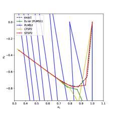
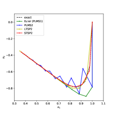
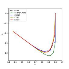
$s=15$
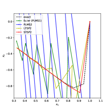
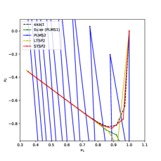
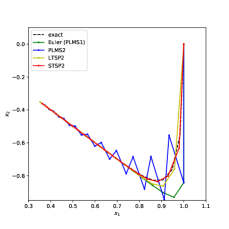
$s=20$
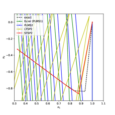
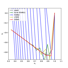
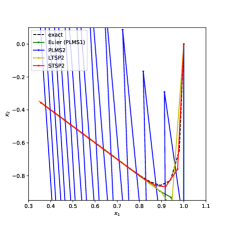
	10 steps	15 steps	20 steps

Figure 17: This figure show how numerical solutions look like when the number of steps are close to the number in Table 9

.

References

- Choi et al. (2021) Jooyoung Choi, Sungwon Kim, Yonghyun Jeong, Youngjune Gwon, and Sungroh Yoon. ILVR: Conditioning method for denoising diffusion probabilistic models. In 2021 IEEE/CVF International Conference on Computer Vision (ICCV), pp. 14347–14356. IEEE, 2021.
- Chung et al. (2022a) Hyungjin Chung, Byeongsu Sim, Dohoon Ryu, and Jong Chul Ye. Improving diffusion models for inverse problems using manifold constraints. In Advances in Neural Information Processing Systems, 2022a.
- Chung et al. (2022b) Hyungjin Chung, Byeongsu Sim, and Jong Chul Ye. Come-Closer-Diffuse-Faster: Accelerating conditional diffusion models for inverse problems through stochastic contraction. In Proceedings of the IEEE/CVF Conference on Computer Vision and Pattern Recognition, pp. 12413–12422, 2022b.
- Crowson (2021) Katherine Crowson. CLIP guided diffusion 512x512, secondary model method. https://twitter.com/RiversHaveWings/status/1462859669454536711, 2021.
- Dhariwal & Nichol (2021) Prafulla Dhariwal and Alexander Nichol. Diffusion models beat GANs on image synthesis. Advances in Neural Information Processing Systems, 34:8780–8794, 2021.
- Dockhorn et al. (2021) Tim Dockhorn, Arash Vahdat, and Karsten Kreis. Score-based generative modeling with critically-damped langevin diffusion. arXiv preprint arXiv:2112.07068, 2021.
- Ernst & Gerhard (2010) Hairer Ernst and Wanner Gerhard. Solving Ordinary Differential Equations. 2: Stiff and Differential Algebraic Problems, volume 2. Springer, 2010.
- Heusel et al. (2017) Martin Heusel, Hubert Ramsauer, Thomas Unterthiner, Bernhard Nessler, and Sepp Hochreiter. GANs trained by a two time-scale update rule converge to a local nash equilibrium. Advances in neural information processing systems, 30, 2017.
- Ho & Salimans (2021) Jonathan Ho and Tim Salimans. Classifier-free diffusion guidance. In NeurIPS 2021 Workshop on Deep Generative Models and Downstream Applications, 2021.
- Ho et al. (2020) Jonathan Ho, Ajay Jain, and Pieter Abbeel. Denoising diffusion probabilistic models. In Proceedings of the 34th International Conference on Neural Information Processing Systems, pp. 6840–6851, 2020.
- Karras et al. (2022) Tero Karras, Miika Aittala, Timo Aila, and Samuli Laine. Elucidating the design space of diffusion-based generative models. In NeurIPS 2022 Workshop on Deep Generative Models and Downstream Applications, 2022.
- Kawar et al. (2022) Bahjat Kawar, Roy Ganz, and Michael Elad. Enhancing diffusion-based image synthesis with robust classifier guidance. arXiv preprint arXiv:2208.08664, 2022.
- Kynkäänniemi et al. (2019) Tuomas Kynkäänniemi, Tero Karras, Samuli Laine, Jaakko Lehtinen, and Timo Aila. Improved precision and recall metric for assessing generative models. Advances in Neural Information Processing Systems, 32, 2019.
- Letts et al. (2021) Adam Letts, Chris Scalf, Alex Spirin, Tom Mason, Chris Allen, Max Ingham, Mike Howles, Nate Baer, and David Sin. Disco diffusion. https://github.com/alembics/disco-diffusion, 2021.
- Li et al. (2022) Wei Li, Xue Xu, Xinyan Xiao, Jiachen Liu, Hu Yang, Guohao Li, Zhanpeng Wang, Zhifan Feng, Qiaoqiao She, Yajuan Lyu, et al. Upainting: Unified text-to-image diffusion generation with cross-modal guidance. arXiv preprint arXiv:2210.16031, 2022.
- Liu et al. (2022) Luping Liu, Yi Ren, Zhijie Lin, and Zhou Zhao. Pseudo numerical methods for diffusion models on manifolds. In International Conference on Learning Representations, 2022.
- Lu et al. (2022) Cheng Lu, Yuhao Zhou, Fan Bao, Jianfei Chen, Chongxuan Li, and Jun Zhu. DPM-Solver: A fast ode solver for diffusion probabilistic model sampling in around 10 steps. In Advances in Neural Information Processing Systems, 2022.
- Luhman & Luhman (2021) Eric Luhman and Troy Luhman. Knowledge distillation in iterative generative models for improved sampling speed. arXiv preprint arXiv:2101.02388, 2021.
- Meng et al. (2021) Chenlin Meng, Yang Song, Jiaming Song, Jiajun Wu, Jun-Yan Zhu, and Stefano Ermon. SDEdit: Guided image synthesis and editing with stochastic differential equations. In International Conference on Learning Representations, 2021.
- Nichol & Dhariwal (2021) Alexander Quinn Nichol and Prafulla Dhariwal. Improved denoising diffusion probabilistic models. In International Conference on Machine Learning, pp. 8162–8171. PMLR, 2021.
- Nichol et al. (2022) Alexander Quinn Nichol, Prafulla Dhariwal, Aditya Ramesh, Pranav Shyam, Pamela Mishkin, Bob Mcgrew, Ilya Sutskever, and Mark Chen. GLIDE: Towards photorealistic image generation and editing with text-guided diffusion models. In International Conference on Machine Learning, pp. 16784–16804. PMLR, 2022.
- Radford et al. (2021) Alec Radford, Jong Wook Kim, Chris Hallacy, Aditya Ramesh, Gabriel Goh, Sandhini Agarwal, Girish Sastry, Amanda Askell, Pamela Mishkin, Jack Clark, et al. Learning transferable visual models from natural language supervision. In International Conference on Machine Learning, pp. 8748–8763. PMLR, 2021.
- Rombach et al. (2022) Robin Rombach, Andreas Blattmann, Dominik Lorenz, Patrick Esser, and Björn Ommer. High-resolution image synthesis with latent diffusion models. In Proceedings of the IEEE/CVF Conference on Computer Vision and Pattern Recognition, pp. 10684–10695, 2022.
- Ruiz et al. (2022) Nataniel Ruiz, Yuanzhen Li, Varun Jampani, Yael Pritch, Michael Rubinstein, and Kfir Aberman. DreamBooth: Fine tuning text-to-image diffusion models for subject-driven generation. arXiv preprint arxiv:2208.12242, 2022.
- Russakovsky et al. (2015) Olga Russakovsky, Jia Deng, Hao Su, Jonathan Krause, Sanjeev Satheesh, Sean Ma, Zhiheng Huang, Andrej Karpathy, Aditya Khosla, Michael Bernstein, et al. Imagenet large scale visual recognition challenge. International journal of computer vision, 115(3):211–252, 2015.
- Salimans & Ho (2022) Tim Salimans and Jonathan Ho. Progressive distillation for fast sampling of diffusion models. In International Conference on Learning Representations, 2022.
- Sasaki et al. (2021) Hiroshi Sasaki, Chris G Willcocks, and Toby P Breckon. Unit-DDPM: Unpaired image translation with denoising diffusion probabilistic models. arXiv preprint arXiv:2104.05358, 2021.
- Song et al. (2020a) Jiaming Song, Chenlin Meng, and Stefano Ermon. Denoising diffusion implicit models. In International Conference on Learning Representations, 2020a.
- Song et al. (2020b) Yang Song, Jascha Sohl-Dickstein, Diederik P Kingma, Abhishek Kumar, Stefano Ermon, and Ben Poole. Score-based generative modeling through stochastic differential equations. In International Conference on Learning Representations, 2020b.
- Strang (1968) Gilbert Strang. On the construction and comparison of difference schemes. SIAM journal on numerical analysis, 5(3):506–517, 1968.
- Trotter (1959) Hale F Trotter. On the product of semi-groups of operators. Proceedings of the American Mathematical Society, 10(4):545–551, 1959.
- Tuckerman (2010) Mark Tuckerman. Statistical mechanics: Theory and molecular simulation. Oxford University Press, 01 2010.
- Wang et al. (2022) Jinyi Wang, Zhaoyang Lyu, Dahua Lin, Bo Dai, and Hongfei Fu. Guided diffusion model for adversarial purification. arXiv preprint arXiv:2205.14969, 2022.
- Watson et al. (2021) Daniel Watson, Jonathan Ho, Mohammad Norouzi, and William Chan. Learning to efficiently sample from diffusion probabilistic models. arXiv preprint arXiv:2106.03802, 2021.
- Wu et al. (2022) Quanlin Wu, Hang Ye, and Yuntian Gu. Guided diffusion model for adversarial purification from random noise. arXiv preprint arXiv:2206.10875, 2022.
- Zhang & Chen (2022) Qinsheng Zhang and Yongxin Chen. Fast sampling of diffusion models with exponential integrator. In NeurIPS 2022 Workshop on Score-Based Methods, 2022.
- Zhang et al. (2022) Qinsheng Zhang, Molei Tao, and Yongxin Chen. gDDIM: Generalized denoising diffusion implicit models. arXiv preprint arXiv:2206.05564, 2022.
- Zhang et al. (2018) Richard Zhang, Phillip Isola, Alexei A Efros, Eli Shechtman, and Oliver Wang. The unreasonable effectiveness of deep features as a perceptual metric. In Proceedings of the IEEE conference on computer vision and pattern recognition, pp. 586–595, 2018.
- Zhao et al. (2022) Min Zhao, Fan Bao, Chongxuan Li, and Jun Zhu. EGSDE: Unpaired image-to-image translation via energy-guided stochastic differential equations. In Advances in Neural Information Processing Systems, 2022.