Fast and accurate determination of the curvature-corrected field emission current

Abstract

The curvature-corrected field emission current density, obtained by linearizing at or below the Fermi energy, is investigated. Two special cases, corresponding to the peak of the normal energy distribution and the mean normal energy, are considered. It is found that the current density evaluated using the mean normal energy results in errors in the net emission current below 3% for apex radius of curvature, $R_{a}\geq 5$nm and for apex fields $E_{a}$ in the range $3-10$ V/nm for an emitter having work-function $\phi=4.5$eV. An analytical expression for the net field emission current is also obtained for locally parabolic tips using the generalized cosine law. The errors are found to be below 6% for $R_{a}\geq 5$nm over an identical range of apex field strengths. The benchmark current is obtained by numerically integrating the current density over the emitter surface and the current density itself computed by integrating over the energy states using the exact Gamow factor and the Kemble form for the WKB transmission coefficient. The analytical expression results in a remarkable speed-up in the computation of the net emission current and is especially useful for large area field emitters having tens of thousands of emission sites.

I Introduction

Recent studies have shown that field emitters with tip radius in the nanometer range can be best modelled accurately by taking into account the variation in local field in the tunneling region, which is roughly 1-2nm from the emitter surface depending on the field strength^{1, 2, 3, 4, 5}. When the apex radius of curvature ($R_{a}$) of the emitter is large ($R_{a}>100$nm), the local field is roughly constant in this region even though the field enhancement factor itself may be large³. Thus, the Murphy-Good current density^{6, 7, 8, 9, 10, 11, 12, 13, 14} is quite likely adequate³ for $R_{a}>100$nm while for emitters with $R_{a}<100$nm, errors first start building up at smaller field strengths and for $R_{a}\leq 10$nm, the errors become large over a wide range of fields^{3, 5}.

The necessity for curvature-corrections was illustrated recently¹ using the experimental results for a single Molybdenum emitter tip² with a FESEM-estimated endcap apex radius of curvature in the 5-10nm range with the square-shaped pyramidal base having a side-length $L_{b}\in[1.25,1.35]\mu$m. Interestingly, even on using the Fowler-Nordheim¹⁶ current density that ignores image-charge contribution and seriously under-predicts the current density, the fit was good^{1, 17} but required an emission area of $130000\text{nm}^{2}$. In contrast, the area of a hemisphere of radius 10nm is only about $628\text{nm}^{2}$. On the other hand¹, the Murphy-Good current density (that takes into account image-charge contribution to the tunneling potential ¹⁵), used with the generalized cosine law^{18, 21} of local field variation around the emitter tip, had a best fit to the experimental data with $R_{a}=9.79$nm which is within the estimated range of $R_{a}$. However, the value of field enhancement required the base-length $L_{b}$ to be $0.65\mu$m which is clearly outside the $1.25-1.35\mu$m range. Thus, while the Fowler-Nordheim current density has gross non-conformity with the physical dimensions, the Murphy-Good current density seems to be in need of a correction. Indeed, on using a curvature-corrected (CC) expression for emission current³, the best fit to experimental data required¹ $R_{a}\approx 5.41$nm and $L_{b}\approx 1.275\mu$m, both of which are within the range of their respective estimated values. This one-off validation could be a coincidence and more such experiments, observation and data analysis are required to explore and put on a firm footing, the limits of validity of each model ^{19, 20}.

The evidence so far seems to suggest that a curvature-corrected field emission theory is necessary for nano-tipped emitters. An elementary form of this³ was used in Ref. [¹], based on a tunneling potential having a single correction term. Since then, an approximately universal tunneling potential having an additional curvature correction term has been established²² using the nonlinear line charge model ^{23, 24, 25, 26, 22} and tested against the finite-element software COMSOL⁴. A curvature-corrected analytical current density has also been determined⁵ by suitably algebraic approximation of the exact Gamow factor and its linearization at the Fermi energy. While the results are promising, there is a scope for improving its accuracy by choosing a different linearization-energy. It is also desirable to have an analytical expression for the net field emission current applicable for $R_{a}\geq 5$nm over a wide range of fields. The present communication seeks to establish accurate analytical expressions for both, the curvature-corrected local current density, as well as the net emission current for smooth locally parabolic emitters.

The issue of accuracy in analytical expressions for current density has recently been investigated in Ref. [¹⁴] for emitters where curvature corrections are unimportant ($R_{a}>100$nm). The three major factors investigated were: (a) the form in which the Gamow factor, $G$, is cast (b) the use of $e^{-G}$ to determine the transmission coefficient and (c) the energy at which the Gamow factor should be linearized in order to obtain an approximate analytical form for the current density. It was found¹⁴ that if an analytical form of the current density is used to determine the net emission current, only the second and third factors are important. For instance, the use of $e^{-G}$ to determine the transmission coefficient leads to errors at larger local fields where the tunneling barrier transitions from ‘strong’ to ‘weak’. A better way of determining the transmission coefficient within the WKB approximation is the Kemble^{28, 29} formula $(1+e^{G})^{-1}$. Another significant cause of error can be ascribed to the energy at which the Gamow factor is linearized in order to obtain an approximate analytical form for the current density. In the traditional approach to cold field emission, the Gamow factor is linearized at the Fermi energy. While this holds at smaller values of the local field, it leads to large errors at higher fields due to the shift in the normal energy distribution away from the Fermi energy. In the following, we shall continue to use the traditional representation of the Gamow factor in term of the Forbes approximation⁷ for the WKB integral, and add curvature corrections to it.

In section II, we shall make use of a curvature-corrected current density that makes use of a Kemble correction and a shifted point of linearization. We shall compare the results by choosing the energy corresponding to the peak of the normal energy distribution as well as the mean normal energy. While both results are encouraging, the mean normal energy is more accurate especially at lower field strengths. Finally, an evaluation of the net field-emission current is carried out using the generalized cosine law in section III and compared with the exact WKB result. Summary and discussions form the concluding section.

II An accurate curvature-corrected current density

A widely adopted method to obtain an analytical expression for the current density is to Taylor expand the Gamow factor about the Fermi energy ${\cal E}_{F}$ in order to carry out the energy integration. Recent studies¹⁴ show that this is adequate at smaller local field strengths for which the electrons closer to the Fermi energy predominantly tunnel through. As the field strength increases, the height and width of the tunneling barrier decreases and the electrons well below the Fermi energy start contributing to the net emitted current. This is evident from the shift in the peak of the normal energy distribution¹³ of the emitted electrons as the local field increases. Hence, for cold field emission, an expansion of the Gamow factor around the peak of the normal energy distribution or the mean normal energy seems preferable. This is likely to yield a better approximation for field emission current density applicable over a wide range of fields.

The use of $e^{-G}$ is also a factor that contributes to the errors at higher fields where the barrier becomes weak. The transmission coefficient in the Kemble form²⁸ can be approximated as¹⁴

$$T({\cal E})=\frac{1}{1+e^{G}}\approx e^{-G}\left[1-e^{-G}\right].$$ (1)

Used alongside the linearization of the Gamow factor, this is likely to provide a simple yet reasonably accurate expression for the field emission current density.

II.1 Expansion of the Gamow factor and the curvature corrected current density

The Gamow factor is expressed as

$$G=g\int_{s_{1}}^{s_{2}}\sqrt{V_{T}(s)-{\cal E}}ds.$$ (2)

Here, $g=2\sqrt{2m}/\hbar$, $m$ the mass of the electron and $\hbar$ the reduced Planck’s constant $h/(2\pi)$. In Eq. (2), $V_{T}$ is the tunneling potential energy, ${\cal E}$ is the normal component of electron energy at the emission surface and $s_{1},s_{2}$ are the zeroes of the integrand. The curvature-corrected form of the tunneling potential energy is ^{30, 4}

$$V_{T}(s)\approx{\cal E}_{F}+\phi+V_{ext}(s)-\frac{B}{s(1+s/2R)}$$ (3)

where, $\phi$ is the work function, ${\cal E}_{F}$ the Fermi energy while the external potential energy $V_{ext}$ takes the form,

$$V_{ext}(s)\approx-qE_{l}s\Big{[}1-\frac{s}{R}+\frac{4}{3}\big{(}\frac{s}{R}\big{)}^{2}\Big{]}$$ (4)

with $q$ the magnitude of electronic charge, $B=q^{2}/(16\pi\epsilon_{0})$, $E_{l}$ the local electric field, and $s$ denoting the normal distance from the surface of the emitter. The quantity $R^{-1}$ is the mean curvature^{31, 32} so that $R$ is the harmonic mean of the principle radii of curvature $R_{1}$ and $R_{2}$ at the emission site i.e. $R=2/(R_{1}^{-1}+R_{2}^{-1})$. The curvature-corrected external potential of Eq. 4 follows directly from Eq. (35) of Ref. [⁴] which holds in the region close to the apex for all axially symmetric emitters in a parallel plate diode configuration. For a more detailed exposition, the reader may refer to appendix A on the tunneling potential³³.

Using the curvature-corrected tunneling potential energy of Eq. (3), an approximate form for the Gamow factor can be found numerically to be⁵

$$G = \frac{2}{3}g\frac{\varphi^{3/2}}{qE_{l}}[\nu(y)+xw_{1}(y)+x^{2}w_{2}(y)+x^{3}w_{3}(y)]$$ (5)

$$= \frac{2}{3}g\frac{\varphi^{3/2}}{qE_{l}}\nu_{c}(y).$$ (6)

Here, $\varphi={\cal E}_{F}+\phi-{\cal E}$, $x=\varphi/(qE_{l}R)$, $y=2\sqrt{qBE_{l}}/\varphi$ and the curvature-corrected barrier function $\nu_{c}(y)=\nu(y)+xw_{1}(y)+x^{2}w_{2}(y)+x^{3}w_{3}(y)$, where⁴

$$\nu(y) = 1-y^{2}+\frac{1}{3}y^{2}\ln y$$ (7)

$$w_{1}(y) = \frac{10}{13}-\frac{2}{11}y^{2}+\frac{1}{80}y^{4}+\frac{1}{200}y^{2}\ln y$$ (8)

$$w_{2}(y) = \frac{10}{11}+\frac{2}{11}y^{2}-\frac{1}{6}y^{4}+\frac{1}{200}y^{2}\ln y$$ (9)

$$w_{3}(y) = -\frac{41}{10}+\frac{39}{20}y^{2}+\frac{1}{3}y^{4}-\frac{1}{150}y^{2}\ln y.$$ (10)

Note that $xw_{1}(y),x^{2}w_{2}(y),x^{3}w_{3}(y)$ are the curvature corrections that arise due to $R$ dependent terms in the external as well as image charge potential. As $R\to\infty$ in the planar limit, $x\to 0$, so that $\nu_{c}(y)$ reduces to $\nu(y)$ which corresponds to the use of the Schottky-Nordheim barrier.

We shall hereafter denote the linearization energy by ${\cal E}_{m}$. On expansion of the curvature-corrected Gamow factor and retaining the linear term, we obtain

$$G({\cal E})\approx G({\cal E}_{m})-({\cal E}-{\cal E}_{m})\frac{t_{\text{cm}}}{d_{m}}$$ (11)

where $t_{\text{cm}}=t_{c}({\cal E}_{m})$ with

$$\begin{split}t_{\text{cm}}&=t(y_{m})+x_{m}t_{1}(y_{m})+x_{m}^{2}t_{2}(y_{m})+x_{m}^{3}t_{3}(y_{m})\\ &=\left(1+\frac{y_{m}^{2}}{9}-\frac{1}{9}y_{m}^{2}\ln y_{m}\right)+\\ &x_{m}\left(\frac{25}{13}-\frac{237}{1100}y_{m}^{2}-\frac{1}{480}y_{m}^{4}-\frac{7}{1200}y_{m}^{2}\ln y_{m}\right)+\\ &x_{m}^{2}\left(\frac{70}{33}+\frac{589}{3300}y_{m}^{2}+\frac{1}{18}y_{m}^{4}+\frac{1}{200}y_{m}^{2}\ln y_{m}\right)+\\ &x_{m}^{3}\left(-\frac{123}{10}+\frac{2929}{900}y_{m}^{2}+\frac{1}{9}y_{m}^{4}-\frac{1}{90}y_{m}^{2}\ln y_{m}\right)\end{split}$$ (12)

where $y_{m}=c_{s}\sqrt{E_{l}}/\varphi_{m}$, $d_{m}^{-1}=g\frac{\varphi_{m}^{1/2}}{E_{l}}$, $c_{s}=1.199985~{}{\rm eV}~{}({\rm V/nm})^{-1/2}$, $\varphi_{m}={\cal E}_{F}+\phi-{\cal E}_{m}$ and $x_{m}=\varphi_{m}/(qE_{l}R)$. The Gamow factor at ${\cal E}_{m}$ can be expressed as

$$G({\cal E}_{m})=B_{\text{FN}}\varphi_{m}^{3/2}\frac{\nu_{\text{cm}}}{E_{l}}$$ (13)

where $\nu_{\text{cm}}=\nu(y_{m})+x_{m}w_{1}(y_{m})+x_{m}^{2}w_{2}(y_{m})+x_{m}^{3}w_{3}(y_{m})$. The field emission current density

$$J = \frac{2mq}{(2\pi)^{2}\hbar^{3}}\int_{0}^{{\cal E}_{F}}({\cal E}_{F}-{\cal E})\frac{1}{1+e^{G({\cal E})}}~{}d{{\cal E}}$$

$$\approx \frac{2mq}{(2\pi)^{2}\hbar^{3}}\int_{0}^{{\cal E}_{F}}({\cal E}_{F}-{\cal E})e^{-G({\cal E})}\left[1-e^{-G({\cal E})}+\ldots\right]~{}d{{\cal E}}$$

can be expressed on completing the integration over energy states as

$$J_{\text{cc}}^{m} \approx A_{\text{FN}}\frac{1}{\varphi_{m}}\frac{E_{l}^{2}}{t_{\text{cm}}^{2}}e^{-{\cal B}_{\text{cc}}}\left(1-\frac{e^{-{\cal B}_{\text{cc}}}}{4}\right)$$ (15)

$${\cal B}_{\text{cc}} = B_{\text{FN}}\varphi_{m}^{3/2}\frac{\nu_{\text{cm}}}{E_{l}}-\frac{t_{\text{cm}}}{d_{m}}({\cal E}_{F}-{\cal E}_{m})$$ (16)

where $A_{\small{\rm FN}}~{}\simeq~{}1.541434~{}{\rm\mu A~{}eV~{}V}^{-2}$, $B_{\small{\rm FN}}~{}\simeq 6.830890~{}{\rm eV}^{-3/2}~{}{\rm V~{}nm}^{-1}$ are the usual Fowler-Nordheim constants. The curvature-corrected current density $J_{\text{cc}}^{m}$ (Eq. (15)), with the incorporation of the first Kemble correction and linearization of the Gamow factor at ${\cal E}_{m}$ provides an analytical expression that can be used to evaluate the net field emission current from a curved emitter, either by numerically integrating over the surface or by using the local field variation over the emitter surface to obtain an approximate analytical expression for the net field emission current.

II.2 Numerical verification

The exact WKB result (referred to hereafter as the benchmark) obtained by (i) finding the Gamow factor exactly by numerical integration (ii) use of the Kemble form of transmission coefficient and (iii) numerical integration over energy to obtain the current density, can be used to validate Eq. (15). Since we shall be comparing net emission currents rather than current-densities, the local current density is integrated over the surface near the apex to obtain the net current numerically.

The geometrical entity we are focusing on is an axially-symmetric emitter having an apex radius of curvature $R_{a}$ and height $h=300R_{a}$. It is mounted on a parallel plate diode where the generalized cosine law^{18, 21} of local field variation holds:

$$E_{l}=E_{a}\frac{z/h}{\sqrt{(z/h)^{2}+(\rho/R_{a})^{2}}}=E_{a}\cos\tilde{\theta}.$$ (17)

In the above, $h$ is the height of the emitter, $R_{a}$ is the apex radius of curvature and $E_{a}$ the apex field. Eq. (17) holds for all axially symmetric emitters where the tips are locally approximated well by a parabola $z\approx h-\rho^{2}/(2R_{a})$ upto $\rho\approx R_{a}$. Thus the only parameters required are $h,R_{a}$ and the apex field^{34, 35, 36, 37} $E_{a}$, since the generalized cosine law^{18, 21} for local fields holds for such emitter-tips. Note that the benchmark also uses the parabolic approximation and the generalized cosine law for determining the net emission current³⁸. In the following, we shall consider ${\cal E}_{F}=8.5$eV and $\phi=4.5$eV. The apex fields considered are in the range [3,10] V/nm which correspond to scaled barrier fields³⁹ $E_{a}/E_{\phi}$ in the range 0.21333 - 0.71109 where $E_{\phi}=(0.6944617~{}\text{eV}^{-2}\text{V}\text{nm}^{-1})\phi^{2}$.

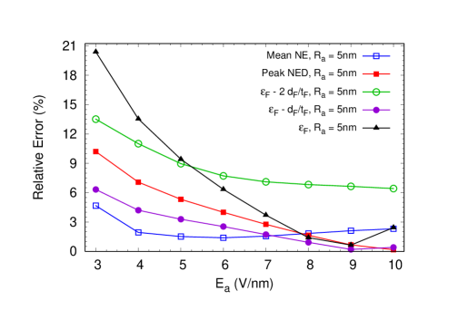
Figure 1: The absolute relative error in the net emission current with respect to the exact WKB result. Five cases are shown with various linearization energy ${\cal E}_{m}$. ‘Mean NE’ refers to the exact mean normal energy, ‘Peak NED’ refers to the exact energy at which the normal energy distribution peaks, ‘${\cal E}_{F}$’ refers to ${\cal E}_{m}={\cal E}_{F}$, ‘${\cal E}_{F}-2d_{F}/t_{F}$’ is the approximate mean normal energy, while ‘${\cal E}_{F}-d_{F}/t_{F}$’ is the approximate peak of the normal energy distribution.

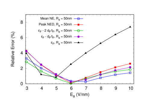
Figure 2: As in case of Fig. 1 with $R_{a}=50$nm. Note that the error for ${\cal E}_{m}={\cal E}_{F}$ increases at higher values of $E_{a}$.

It is clear that there are severals factors at play when comparing the error with respect to the exact WKB result. We shall discuss two of these from the broad picture available to us. The first is the effect of curvature correction which reflects in the approximate Gamow factor in Eq. (5). Since the expansion is in powers of $x=\varphi/(qE_{l}R)$, the approximate Gamow factor is prone to errors at smaller values of $E_{l}$ and $R$. Thus, irrespective of the energy at which the linearization is carried out, lower fields and radius of curvature are prone to errors. In general, at higher $R$ and $E_{l}$, the curvature errors are expected to reduce. The second important consideration is the energy at which the linearization is carried out. Since the peak of the normal energy distribution moves away from ${\cal E}_{F}$ at higher fields for a given $R_{a}$, linearization at ${\cal E}_{m}={\cal E}_{F}$ should in general lead to larger errors at higher fields strengths. Apart from these two, there are other subtle effects that decide the magnitude of relative error at a given field strength as we shall see. Note that on the surface of an emitter, $E_{l}$ reduces away from the apex while $R$ increases and this leads to a mild decrease in the expansion parameter $x$.

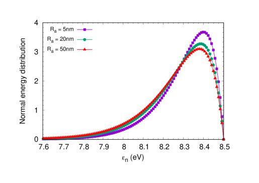
Figure 3: The normal energy distribution at $E_{a}=3$V/nm for $R_{a}=5,~{}20~{}\text{and}~{}50$nm. Note the shift in the distribution away from the ${\cal E}_{F}$ (= 8.5eV here) for larger values of $R_{a}$.

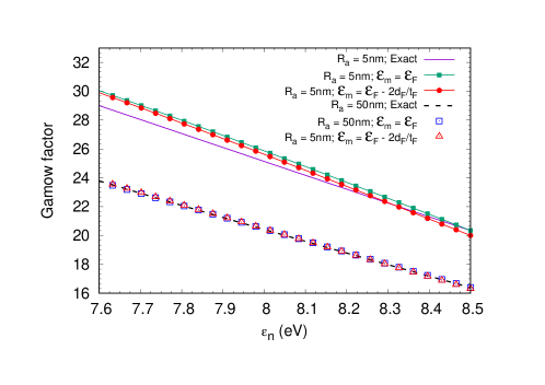
Figure 4: The exact Gamow factor at $E_{a}=3$V/nm is compared with the linearized Gamow factors with the point of linearization at ${\cal E}_{m}={\cal E}_{F}$ and ${\cal E}_{m}={\cal E}_{F}-2d_{F}/t_{F}$. The upper set of curves correspond to $R_{a}=5$nm while the lower set is for $R_{a}=50$nm. The two linearized versions are nearly equivalent at $R_{a}=50$nm while, for $R_{a}=5$nm linearizing at the approximate mean energy yields results closer to the exact Gamow factor over the energy range of interest.

With this perspective, we shall compare the absolute relative errors at $R_{a}=5$nm and $R_{a}=50$nm shown in Figs. 1 and 2 respectively, for various values of ${\cal E}_{m}$ displayed in the legends. Clearly ‘Mean NE’, which refers to the exact mean normal energy determined numerically (see appendix C), performs well at $R_{a}=5$nm at all field strengths while ${\cal E}_{m}={\cal E}_{F}$ shows large errors especially at lower fields. Even at $R_{a}=50$nm where curvature errors are expected to be smaller, ‘Mean NE’ as well as the approximate mean normal energy (${\cal E}_{m}\approx{\cal E}_{F}-2d_{F}/t_{F}$) perform well while in case of ${\cal E}={\cal E}_{F}$, the linearization error dominates leading to larger errors at higher field strengths. The energy value corresponding to the peak of the normal energy distribution (‘Peak NED’) also gives good results though the errors are somewhat high for smaller apex fields at $R_{a}=5$nm.

Some of the trends in Figs. 1 and 2 are easy to understand. For instance, at $R_{a}=5$nm, the errors fall as expected with an increase in $E_{a}$ in all cases (except for a mild increase at ${\cal E}_{m}={\cal E}_{F}$ for $E_{a}>9$V/nm). The larger than expected error (approximately $21\%$) for ${\cal E}_{m}={\cal E}_{F}$ at $E_{a}=3$V/nm however seems intriguing. To understand this better, the normal energy distribution (see Fig. 3) for different values of $R_{a}$ at $E_{a}=3$V/nm is quiet instructive. The peak of the normal energy distribution shifts slightly away from ${\cal E}_{F}$ as $R_{a}$ increases. Note also that the distributions have a long tail. The linearized Gamow factor in the corresponding normal energy range is shown in Fig. 4. For $R_{a}=5$nm, linearization at ${\cal E}_{F}$ results in larger deviations from the exact Gamow factor compared to linearization at ${\cal E}_{F}-2d_{F}/t_{F}$. Not surprisingly, the relative error in net emission current drops from about $21\%$ to about $13\%$ in moving from ${\cal E}_{m}={\cal E}_{F}$ to ${\cal E}_{m}={\cal E}_{F}-2d_{F}/t_{F}$.

At $R_{a}=50$nm, curvature effects are smaller and the linearized Gamow factor does not noticeably deviate from the exact Gamow factor (see Fig. 4 for $E_{a}=3$V/nm). Thus, the errors remain more or less similar at all linearization energies. The magnitude of the error at a particular $E_{a}$ depends on how closely the linearized Gamow factor approximates the exact Gamow factor over the relevant range of normal energies. For $E_{a}>5$V/nm at ${\cal E}_{m}={\cal E}_{F}$, the increase in error is expected due to the shift in normal energy distribution away from ${\cal E}_{F}$ and the corresponding deviation of the linearized Gamow factor from the exact Gamow factor.

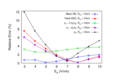
Figure 5: As in case of Fig. 1 with $R_{a}=10$nm.

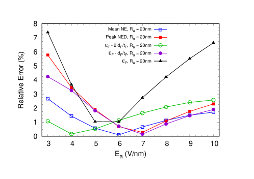
Figure 6: As in case of Fig. 1 with $R_{a}=20$nm.

In order to verify that the trend observed in moving from $R_{a}=5$nm to $R_{a}=50$nm is gradual, we show the results for $R_{a}=10$nm and $R_{a}=20$nm in Figs. 5 and 6. It is apparent from these results that linearization at the exact mean normal energy (‘Mean NE’) is optimum for all values of $R_{a}$ and $E_{a}$ with errors generally below $3\%$. The approximate mean normal energy ${\cal E}_{m}\approx{\cal E}_{F}-2d_{F}/t_{F}$ is only marginally worse with errors exceeding 6% only at $R_{a}=5$nm.

III The net curvature-corrected emission current

The curvature-corrected expression for the current density, with linearization at the mean normal energy, can be used to arrive at an analytical expression for the net emission current on using the generalized cosine law of local field variation $E_{l}=E_{a}\cos\tilde{\theta}$ (Eq. (17)). Assuming a sharp locally parabolic emitter tip, the total emitted current can be evaluated using the expression¹³

$$I\approx 2\pi R_{a}^{2}\int J_{\text{cc}}(\tilde{\theta})\frac{\sin\tilde{\theta}}{\cos^{4}\tilde{\theta}}\times{\cal C}(\tilde{\theta})~{}d\tilde{\theta}$$ (18)

where ${\cal C}(\tilde{\theta})$ is a correction factor which, for a sharp emitter ($h/R_{a}>>1$), is approximately unity. In the following we shall assume the emitter to be reasonably sharp so that ${\cal C}\approx 1$.

The basic idea is to express $J_{\text{cc}}$ in terms of $\tilde{\theta}$ by replacing all the local fields using $E_{l}=E_{a}\cos\tilde{\theta}$. A further simplification can be made by the substitution $1/\cos\tilde{\theta}=1+u$ and retaining only terms upto ${\mathcal{O}(u^{2})}$ in ${\cal B}_{\text{cc}}$ and $t_{\text{cm}}^{-2}$. The approximation is expected to be good at lower apex fields since the emission is limited to an area closer to the apex, while at higher fields, where the emission area is larger, this might lead to larger errors.

Writing ${\cal B}_{\text{cc}}\approx D_{0}+D_{1}u$ and $t_{\text{cm}}^{-2}\approx F_{0}+F_{1}u$, the integration can be carried out easily. Note that, it generally suffices to integrate upto $\rho=R_{a}$ which, for a sharp emitter, corresponds to $\tilde{\theta}=\pi/4$ or $u=\sqrt{2}-1=u_{\text{0}}$. Thus,

$$I\approx 2\pi R_{a}^{2}{\cal G}A_{\text{FN}}\frac{1}{\varphi_{\text{ma}}}E_{a}^{2}F_{0}e^{-D_{0}}$$ (19)

where ${\cal E}_{m}$ is the mean normal energy, while

$$\begin{split}{\cal G}\approx&\frac{1}{D_{1}}+\frac{F_{1}}{F_{0}}\frac{1}{D_{1}^{2}}-\frac{e^{-D_{0}}}{4}\left(\frac{1}{2D_{1}}+\frac{F_{1}}{F_{0}}\frac{1}{4D_{1}^{2}}\right)-\\ &e^{-D_{1}u_{\text{0}}}\left[\frac{1}{D_{1}}+\frac{F_{1}}{F_{0}}\frac{1+D_{1}u_{\text{0}}}{D_{1}^{2}}-\frac{e^{-D_{0}-D_{1}u_{\text{0}}}}{4}\times\right.\\ &\left.~{}~{}~{}~{}~{}~{}~{}~{}~{}~{}\left(\frac{1}{2D_{1}}+\frac{F_{1}}{F_{0}}\frac{1+2D_{1}u_{\text{0}}}{4D_{1}^{2}}\right)\right].\end{split}$$ (20)

Expressions for $D_{0},D_{1},F_{0}$ and $F_{1}$ can be found in appendix B.

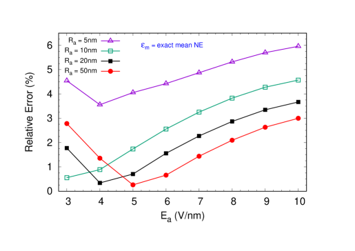
Figure 7: The magnitude of the relative error in the analytical expression for the curvature-corrected current (Eq. 19) compared to the exact WKB result. Here ${\cal E}_{m}$ is the exact mean normal energy.

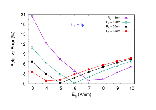
Figure 8: The magnitude of the relative error in the analytical expression for the curvature-corrected current (Eq. 19) compared to the exact WKB result for ${\cal E}_{m}={\cal E}_{F}$.

In Fig. 7, we compare the magnitude of the relative error in the net current as given by Eq. (19) and (20) with respect to the exact WKB result which has been used as the benchmark throughout this study with ${\cal E}_{m}$ as the exact mean normal energy. Clearly, the analytical expression is adequate for a wide range of fields and apex radius of curvature. The increase in error at higher fields is due to the linearization of ${\cal B}_{\text{cc}}$ and $t_{\text{cm}}^{-2}$ in the variable $u$ which is a measure of the distance from the apex. This is however a small price to pay for a compact analytical expression for the net emission current.

For the sake of comparison, we also show the relative errors in the net current obtained using the analytical expressions in Eq. (19) and (20) with ${\cal E}_{m}={\cal E}_{F}$. The trends are similar to those shown in section II.2 where the linearized current density is integrated numerically over the emitter end-cap. The errors are more pronounced at smaller apex radius of curvature and apex field strengths. Clearly, linearization at the mean normal energy ensures smaller errors over a wide range of fields and radius of curvature.

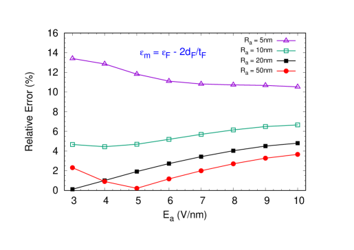
Figure 9: The magnitude of the relative error in the analytical expression for the curvature-corrected current (Eq. 19) compared to the exact WKB result. Here, ${\cal E}_{m}={\cal E}_{F}-2d_{F}/t_{F}$.

While the errors are reasonably small when the exact mean normal energy is used, it require the computation of integrals that marginally offsets the use of an analytical expression for the net current. In Fig. 9, we provide a comparison of the magnitude of relative errors with respect to the exact WKB result, using the approximate ${\cal E}_{m}={\cal E}_{F}-2d_{F}/t_{F}$. While the errors for $R_{a}=5$nm are somewhat large, the approximate value of the mean normal energy may be used profitably for $R_{a}\geq 10$nm.

Table 1: Comparison of time required for $10000$ evaluations of the net emission current for $E_{a}\in[3,10]$V/nm and $R_{a}\in[5,50]$nm. The ‘Scale Factor’ is the ratio of the time taken by ‘WKB Exact’ and the time taken by a given method. It gives a rough indication of the speed-up achieved. Here ${\cal E}_{m}$ is the mean normal energy. Also shown is the average relative error with respect to ‘WKB exact’.

Method	Time (s)	Scale Factor	Average Error
WKB Exact	315.1 s	1	—
WKB Fit	23.8 s	13.24	1.67%
Eq. (19) with	56.7 s	5.55	2.06%
${\cal E}_{m}$ exact
Eq. (19) with	0.0003 s	$10^{6}$	3.14%
${\cal E}_{m}$ approximate

Finally, Table 1 provides a comparison of the CPU time (in seconds) required on a standard desktop to serially compute the net emission current for $10^{4}$ combinations of $E_{a}$ and $R_{a}$ in the range of apex fields and radius of curvature considered in this paper. Thus, there are 100 values of $R_{a}$ spaced uniformly in the range [5,50]nm and 100 values of $E_{a}$ spaced uniformly in the [3,10]V/nm range. In the table, ‘WKB Fit’ refers to the use of Eq. (5) for the Gamow factor and numerical integration over energy while ‘WKB exact’ refers to the ‘exact’ numerical evaluation of the Gamow factor followed by numerical integration over energy. The last two rows refer to the analytical formula for the net current of Eq. (19) with ‘${\cal E}_{m}$ exact’ evaluated as outlined in appendix C and ‘${\cal E}_{m}$ approximate’ as ${\cal E}_{m}\approx{\cal E}_{F}-2d_{F}/t_{F}$. Clearly, linearization at the approximate mean normal energy results in fast computation of the net emission current using Eq. (19) by a factor $\approx 80000$ compared to ‘WKB fit’ and about $10^{6}$ compared to the ‘WKB exact’ result. This is only marginally offset by a larger error for $R_{a}=5$nm as seen in Fig. 9. The average relative error in the $5-50$nm range is however small as shown in Table 1.

IV Conclusions

We have presented an expression for the curvature-corrected current density obtained by linearization at an energy ${\cal E}_{m}\leq{\cal E}_{F}$ and insertion of a correction term to account for the Kemble transmission coefficient. Numerical results show that the mean normal energy is a suitable candidate for the linearization energy ${\cal E}_{m}$ and predicts the net emission current to within 3% accuracy compared to the exact WKB result for $R_{a}\geq 5$nm and over a wide range of field.

We have also obtained an analytical expression for the net emission current using the generalized cosine law of local field variation. It requires only the apex radius of curvature $R_{a}$ and the apex electric field $E_{a}$ and is able to calculate the net field-emission current to within 6% accuracy compared to the current obtained by explicitly integrating the exact WKB current density over the emitter tip for $R_{a}\geq 5$nm and a wide range of apex fields.

Both of these results are expected to be useful in dealing with sharp emitters having tip radius $R_{a}\geq 5$nm. The expression for current density can be used in all situations including those where the emitter does not have any special symmetry. On the other hand, the expression for the net emission current is extremely useful for axially symmetric emitters with smooth locally parabolic tips mounted in a parallel plate configuration, considering that the speed-up achieved in current computation is enormous. The accuracies obtained in all cases are good, given that even minor experimental uncertainties can lead to far larger changes in the net emission current.

Finally, the analytical expression for emission current is especially useful for a fast determination of net emission current from a large area field emitter have thousands of axially symmetric emitters ^{40, 41, 42}.

V Author Declarations

V.1 Conflict of interest

There is no conflict of interest to disclose.

V.2 Data Availability

The data that supports the findings of this study are available within the article.

V.3 Author Contributions

Debabrata Biswas Conceptualization (lead), data curation (equal), formal analysis (equal), methodology (lead), software (equal), validation (supporting), visualization (equal), original draft (lead), review and editing (supporting).

Rajasree Ramachandran Conceptualization (supporting), data curation (equal), formal analysis (equal), methodology (supporting), software (equal), validation (lead), visualization (equal), original draft (supporting), review and editing (lead).

VI Reference

Appendix A The tunneling potential

The electric field, $E_{l}$, close to the emitter surface is assumed to be a constant so that the corresponding potential can be expressed as $V_{ext}(s)=-E_{l}s$ where $s$ is the normal distance from the surface of the emitter and $E_{l}$ is the magnitude of the local electric field. The assumption holds good when the radius of curvature at the emission site is large (typically $R>100$nm).

As $R$ decreases, corrections become important and these can be expressed as powers of $s/R$. Thus,

$$V_{ext}(s)=-E_{l}s\left[1+c_{1}\frac{s}{R}+\ldots+c_{n}\left(\frac{s}{R}\right)^{n}+\ldots\right].$$ (21)

The effective spherical approximation used in Ref. [³²] leads to $c_{n}=(-1)^{n}$ so that $V_{ext}(s)=-E_{l}R\left[1-1/(1+s/R)\right]$ with $R^{-1}=2/(R_{1}^{-1}+R_{2}^{-1})$. In Ref. [³⁰], following the analysis of the hemiellipsoid, the hyperboloid and the hemisphere, it was concluded that $c_{1}=-1$, $c_{2}=4/3$ and $R\approx R_{2}$ where $R_{2}$ is the second (smaller) principle radius of curvature. With these identifications, the external potential was found to approximate the numerically determined external potentials for other emitter shapes as well³⁰. Ref. [⁴] uses the nonlinear line charge model²² for axially symmetric emitters to arrive at an approximate form close to the apex. In the following, we shall show that the results of both Ref. [³⁰, ⁴] can be recast in the form where {$c_{1}=-1$, $R=R_{m}$} exactly while {$c_{2}=4/3$, $R^{2}=R_{m}^{2}$} is approximate but fairly accurate close to the apex.

In addition to the approximate results in section II³⁰, Ref. [³⁰] also provides in the appendix, a systematic expansion of the external potential in powers of $s$ for the hemi-ellipsoid. In terms of the prolate spheroidal co-ordinates ($\eta,\xi,\varphi)$

$$x = L\sqrt{(\eta^{2}-1)(1-\xi^{2})}\cos\varphi$$ (22)

$$y = L\sqrt{(\eta^{2}-1)(1-\xi^{2})}\sin\varphi$$ (23)

$$z = L\eta\xi$$ (24)

it was found that

$$V_{ext}(s)=V(s)=\left[d_{1}s+d_{2}s^{2}+d_{3}s^{3}\right]$$ (25)

where

$$d_{1} = V_{\eta}a_{1}$$ (26)

$$d_{2} = V_{\eta}a_{2}+\frac{1}{2}V_{\eta\eta}a_{1}^{2}$$ (27)

$$d_{3} = V_{\eta}a_{3}+V_{\eta\eta}a_{1}a_{2}+V_{\xi\eta}a_{1}b_{2}+\frac{1}{6}V_{\eta\eta\eta}a_{1}^{3}.$$ (28)

The derivatives of the potential at a point ($\eta_{0},\xi_{0}$) on the surface of the hemiellipsoid are

$$V_{\eta} = E_{l}h_{\eta}$$ (29)

$$V_{\eta\eta} = -E_{l}h\eta\frac{2\eta_{0}}{\eta_{0}^{2}-1}$$ (30)

$$V_{\eta\xi} = E_{l}h_{\eta}\frac{1}{\xi_{0}}$$ (31)

$$V_{\eta\eta\eta} = E_{l}h_{\eta}\frac{8\eta_{0}^{2}}{(\eta_{0}^{2}-1)^{2}}$$ (32)

where

$$h_{\eta} = L\sqrt{(\eta_{0}^{2}-\xi_{0}^{2})/(\eta_{0}^{2}-1)}$$ (33)

$$h_{\xi} = L\sqrt{(\eta_{0}^{2}-\xi_{0}^{2})/(1-\xi_{0}^{2})}.$$ (34)

The coefficients

$$a_{1} = \frac{1}{h_{\eta}}$$ (35)

$$a_{2} = \frac{1}{2h_{\xi}^{2}}\frac{\eta_{0}}{\eta_{0}^{2}-\xi_{0}^{2}}$$ (36)

$$a_{3} = -\frac{1}{2h_{\eta}h_{\xi}^{2}}\frac{\eta_{0}^{2}+\xi_{0}^{2}}{(\eta_{0}^{2}-\xi_{0}^{2})^{2}}$$ (37)

$$b_{2} = -\frac{1}{2h_{\xi}^{2}}\frac{\xi_{0}}{\eta_{0}^{2}-\xi_{0}^{2}}$$ (38)

while the principle radii of curvature are

$$R_{1} = R_{a}\frac{(\eta_{0}^{2}-\xi_{0}^{2})^{3/2}}{(\eta_{0}^{2}-1)^{3/2}}$$ (39)

$$R_{2} = R_{a}\frac{(\eta_{0}^{2}-\xi_{0}^{2})^{1/2}}{(\eta_{0}^{2}-1)^{1/2}}$$ (40)

where $R_{a}$ is the apex radius of curvature. On putting together these results, the values of $d_{1},d_{2}$ and $d_{3}$ are

$$d_{1} = -E_{l}$$ (41)

$$d_{2} = \frac{E_{l}}{2R_{a}}\frac{(\eta_{0}^{2}-1)^{1/2}}{(\eta_{0}^{2}-\xi_{0}^{2})^{3/2}}\left[2\eta_{0}^{2}-1-\xi_{0}^{2}\right]$$ (42)

$$= \frac{E_{l}}{R_{m}}$$

$$d_{3} = -\frac{4}{3}\frac{E_{l}}{R_{m}^{2}}\frac{\left[3+4\eta_{0}^{4}+\xi_{0}^{4}-2\eta_{0}^{2}(3+\xi_{0}^{2})\right]}{(1+\xi_{0}^{2}-2\eta_{0}^{2})^{2}}$$ (43)

$$= -\frac{4}{3}\frac{E_{l}}{R_{m}^{2}}\left[1-2\frac{(\eta_{0}^{2}-1)(1-\xi_{0}^{2})}{(1+\xi_{0}^{2}-2\eta_{0}^{2})^{2}}\right]$$ (44)

$$= -\frac{4}{3}\frac{E_{l}}{R_{m}^{2}}\left[1-\cal{C}\right]$$ (45)

where

$$R_{m} = \frac{2}{(1/R_{1}+1/R_{2})}$$ (46)

$$= 2R_{a}\frac{\eta_{0}^{2}-\xi_{0}^{2})^{3/2}}{(\eta_{0}^{2}-1)^{1/2}(2\eta_{0}^{2}-1-\xi_{0}^{2})}.$$

The external potential thus takes the form

$$V_{ext}(s)=-E_{l}s\left[1-\left(\frac{s}{R_{m}}\right)+\frac{4}{3}\left(\frac{s}{R_{m}}\right)^{2}\left(1-{\cal{C}}\right)\right]$$ (47)

for the hemiellipsoid emitter. In terms of $\rho_{0}^{2}=x_{0}^{2}+y_{0}^{2}$ where $x_{0},y_{0}$ are on the surface of the hemiellipsoid, the correction term ${\cal{C}}=\rho_{0}^{2}/(2R_{a}^{2})$. Thus,

$$V_{ext}(s)=-E_{l}s\left[1-\frac{s}{R_{m}}+\frac{4}{3}\frac{s^{2}}{R_{m}^{2}}\left(1-\frac{1}{2}\frac{\rho_{0}^{2}}{R_{a}^{2}}\right)\right].$$ (48)

Note that close to the apex, $\rho/R_{a}<<1$ while $R_{m}\approx R_{2}$.

A more general result, valid for all axially symmetric emitters in a parallel plate geometry, was arrived at using the nonlinear line charge model⁴. In such cases, the external potential can be expressed as (see Eq. (35) of Ref [⁴]),

$$V_{ext}(s)\approx-E_{l}s\left[1-\frac{s}{R_{a}}(1-\frac{\rho_{0}^{2}}{R_{a}^{2}})+\frac{4}{3}\frac{s^{2}}{R_{a}^{2}}(1-\frac{5}{2}\frac{\rho_{0}^{2}}{R_{a}^{2}})\right].$$ (49)

Close to the apex $1/R_{m}\approx(1/R_{a})(1-\rho_{0}^{2}/R_{a}^{2})$ while $1/R_{m}^{2}\approx(1/R_{a}^{2})(1-2\rho_{0}^{2}/R_{a}^{2})$. Thus, Eq. (49) can be expressed as

$$V_{ext}(s)\approx-E_{l}s\left[1-\frac{s}{R_{m}}+\frac{4}{3}\frac{s^{2}}{R_{m}^{2}}(1-\frac{1}{2}\frac{\rho_{0}^{2}}{R_{a}^{2}})\right].$$ (50)

This is identical to the result obtained for the hemiellipsoid (see Eq. 48) but applicable generally for all axially symmetric emitters. Approximating $(1-\rho_{0}^{2}/(2R_{a}^{2}))\approx 1$ leads us to an approximate universal form for the external potential (see Eq. (4)) close to the emitter surface.

Note that Eq. (49) can also be expressed as

$$V_{ext}(s)\approx-E_{l}s\left[1-\frac{s}{R_{m}}+\frac{4}{3}\frac{s^{2}}{R_{1}R_{m}}\right]$$ (51)

The correction terms, $\frac{s}{R_{m}}$ and $\frac{4}{3}\frac{s^{2}}{R_{1}R_{m}}$ are exact for any point on the hemiellipsoid surface. For other emitter shapes⁴, the two correction terms may have extra factors that can be ascribed to the non-linear line charge distribution. Since these have been ignored as an approximation, we choose to adopt the form in Eq. (4) with $R=R_{m}$ as an approximate but accurate representation of the external potential in the tunneling region.

Finally, while the change from $R_{2}$ to $R_{m}$ reduces the need for approximations, its impact on the net field emission current is small compared to a neglect of the second correction term $4s^{2}/(3R_{m}^{2})$, especially at smaller values of $R_{a}$ and $E_{a}$. For instance, at $R_{a}=5$nm and workfunction $\phi=4.5$eV, the error in net emission current on using $R_{2}$ in Eq. (4) is about 13% at $E_{a}=5$V/nm, while it is around 62% on ignoring $4s^{2}/(3R_{m}^{2})$ altogether. At $E_{a}=4$V/nm, the error in net emission current on using $R_{2}$ in Eq. (4) remains roughly the same while the error grows to around 92% on ignoring $4s^{2}/(3R_{m}^{2})$. In each of these cases, the exact WKB method is used and the benchmark current is obtained using $R_{m}$ in Eq. (4).

Appendix B The coefficients $\bf{D_{0},D_{1},F_{0}}$ and $\bf{F_{1}}$

We shall briefly outline the derivation of the coefficients $D_{0},D_{1},F_{0}$ and $F_{1}$ and state the results. The dependence on $u$ in ${\cal B}_{\text{cc}}$ and $t_{\text{cm}}$ arise from the variation in $E_{l}$ and $x_{m}$ over the surface of the emitter. Thus,

$${\cal B}_{\text{cc}}={\cal B}_{\text{cc}}(E_{l},x_{m})={\cal B}_{\text{cc}}(\frac{E_{a}}{1+u},\frac{x_{\text{ma}}}{1+u})\approx D_{0}+D_{1}u$$ (52)

so that $D_{0}={\cal B}_{\text{cc}}(E_{a},x_{\text{ma}})$. In the above, $x_{m}=\varphi_{m}/(qE_{l}R_{m})\approx x_{\text{ma}}/(1+u)$ where $x_{\text{ma}}=\varphi_{m}/(qE_{a}R_{a})$. The approximation holds for tall emitters where $E_{l}=E_{a}(z/h)/\sqrt{(z/h)^{2}+(\rho/R_{a})^{2}}\approx E_{a}/\sqrt{1+\rho^{2}/R_{a}^{2}}$. The coefficient $D_{1}$ can be written as

$$D_{1} = \left(\frac{d{\cal B}_{\text{cc}}}{du}\right)_{{u=0}}=\left(\frac{dE_{l}}{du}\right)_{{u=0}}\times\left(\frac{d{\cal B}_{\text{cc}}}{dE_{l}}\right)_{E_{l}=E_{a}}$$ (53)

$$+ \left(\frac{dx_{m}}{du}\right)_{{u=0}}\times\left(\frac{d{\cal B}_{\text{cc}}}{dx_{m}}\right)_{x_{m}=x_{\text{ma}}}.$$

Since $E_{l}=E_{a}/(1+u)$, $(dE_{l}/du)_{u=0}=-E_{a}$. Similarly, since $x_{m}=x_{\text{ma}}/(1+u)$, $(dx_{m}/du)_{u=0}=-x_{\text{ma}}$. Thus,

$$D_{1}=-E_{a}(d{\cal B}_{\text{cc}}/dE_{l})_{E_{l}=E_{a}}-x_{\text{ma}}(d{\cal B}_{\text{cc}}/dx_{m})_{x_{m}=x_{\text{ma}}}$$ (54)

This can be further expressed as

$$\begin{split}D_{1}&={\cal B}_{\text{cc}}(E_{a})-\frac{B_{\text{FN}}\varphi_{m}^{3/2}}{E_{a}}\left[E_{a}\frac{d\nu_{\text{cm}}}{dE_{l}}\Big{|}_{E_{a}}+x_{\text{ma}}\frac{d\nu_{\text{cm}}}{dx_{m}}\Big{|}_{x_{\text{ma}}}\right]\\ &+\frac{g\varphi_{m}^{1/2}({\cal E}_{F}-{\cal E}_{m})}{E_{a}}\left[E_{a}\frac{dt_{\text{cm}}}{dE_{l}}\Big{|}_{E_{a}}+x_{\text{ma}}\frac{dt_{\text{cm}}}{dx_{m}}\Big{|}_{x_{\text{ma}}}\right].\end{split}$$ (55)

It is simpler to express $d\nu_{\text{cm}}/dE_{l}$ and $dt_{\text{cm}}/dE_{l}$ as

$$\frac{d\nu_{\text{cm}}}{dE_{l}}\Big{|}_{E_{a}} = \frac{d\nu_{\text{cm}}}{d(y^{2})}\Big{|}_{y_{\text{ma}}}\frac{d(y^{2})}{dE_{l}}\Big{|}_{E_{a}}$$ (56)

$$\frac{dt_{\text{cm}}}{dE_{l}}\Big{|}_{E_{a}} = \frac{dt_{\text{cm}}}{d(y^{2})}\Big{|}_{y_{\text{ma}}}\frac{d(y^{2})}{dE_{l}}\Big{|}_{E_{a}}$$ (57)

and use the fact that $d(y^{2})/dE_{l}=4qB/\varphi_{m}^{2}$. The quantities $\frac{d\nu_{\text{cm}}}{dx_{m}}\Big{|}_{x_{\text{ma}}}$ and $\frac{dt_{\text{cm}}}{dE_{l}}\Big{|}_{x_{\text{ma}}}$ can be obtained directly and expressed as

$$\frac{d\nu_{\text{cm}}}{dx_{m}}\Big{|}_{x_{\text{ma}}} = w_{1}(y_{\text{ma}})+2x_{\text{ma}}w_{2}(y_{\text{ma}})+3x_{\text{ma}}^{2}w_{3}(y_{\text{ma}})$$

$$\frac{dt_{\text{cm}}}{dx_{m}}\Big{|}_{x_{\text{ma}}} = t_{1}(y_{\text{ma}})+2x_{\text{ma}}t_{2}(y_{\text{ma}})+3x_{\text{ma}}^{2}t_{3}(y_{\text{ma}}).$$

These results can be combined to obtain

$$\begin{split}&D_{1}={\cal B}_{\text{cc}}(E_{a})\\ &-B_{\text{FN}}\frac{4qB}{\varphi_{m}^{1/2}}\frac{d\nu_{\text{cm}}}{d(y^{2})}\Big{|}_{y_{\text{ma}}^{2}}+\frac{4Bqg({\cal E}_{F}-{\cal E}_{m})}{\varphi_{m}^{3/2}}\frac{dt_{\text{cm}}}{d(y^{2})}\Big{|}_{y_{\text{ma}}^{2}}\\ &-\frac{B_{\text{FN}}\varphi_{m}^{3/2}}{E_{a}}x_{\text{ma}}\frac{d\nu_{\text{cm}}}{dx_{m}}\Big{|}_{x_{\text{ma}}}+\frac{({\cal E}_{F}-{\cal E}_{m})}{d_{\text{ma}}}x_{\text{ma}}\frac{dt_{\text{cm}}}{dx_{m}}\Big{|}_{x_{\text{ma}}}\end{split}$$ (58)

where $y_{\text{ma}}^{2}=4qBE_{a}/\varphi_{m}^{2}$. Finally,

$$\begin{split}~{}~{}~{}&\left(\frac{d\nu_{\text{cm}}}{d(y^{2})}\right)_{y^{2}=y_{\text{ma}}^{2}}=\\ &u_{0}(y_{\text{ma}})+x_{\text{ma}}u_{1}(y_{\text{ma}})+x_{\text{ma}}^{2}u_{2}(y_{\text{ma}})+x_{\text{ma}}^{3}u_{3}(y_{\text{ma}})\end{split}$$ (59)

with

$$u_{0}(y_{\text{ma}}) = -1+\frac{1}{6}(1+\ln y_{\text{ma}}^{2})+\frac{1}{6}$$ (60)

$$u_{1}(y_{\text{ma}}) = -\frac{2}{11}+\frac{2}{80}y_{\text{ma}}^{2}+\frac{1}{400}(1+\ln y_{\text{ma}}^{2})$$ (61)

$$u_{2}(y_{\text{ma}}) = \frac{2}{11}+\frac{2}{3}y_{\text{ma}}^{2}+\frac{1}{400}(1+\ln y_{\text{ma}}^{2})$$ (62)

$$u_{3}(y_{\text{ma}}) = \frac{39}{20}+\frac{2}{3}y_{\text{ma}}^{2}-\frac{1}{300}(1+\ln y_{\text{ma}}^{2}).$$ (63)

Similarly,

$$\begin{split}~{}~{}~{}&\left(\frac{dt_{\text{cm}}}{d(y^{2})}\right)_{y^{2}=y_{\text{ma}}^{2}}=\\ &p_{0}(y_{\text{ma}})+x_{\text{ma}}p_{1}(y_{\text{ma}})+x_{\text{ma}}^{2}p_{2}(y_{\text{ma}})+x_{\text{ma}}^{3}p_{3}(y_{\text{ma}})\end{split}$$ (64)

with

$$p_{0}(y) = \frac{1}{9}-\frac{1}{18}(1+\ln y^{2})+\frac{1}{6}$$ (65)

$$p_{1}(y) = -\frac{237}{1100}-\frac{1}{240}y^{2}-\frac{7}{2400}(1+\ln y^{2})$$ (66)

$$p_{2}(y) = \frac{589}{3300}+\frac{1}{9}y^{2}+\frac{1}{400}(1+\ln y^{2})$$ (67)

$$p_{3}(y) = \frac{2929}{900}+\frac{2}{9}y^{2}-\frac{1}{45}(1+\ln y^{2}).$$ (68)

This completes the evaluation of $D_{1}$ in Eq. (58).

The coefficients $F_{0}$ and $F_{1}$ are defined as

$$\frac{1}{t_{\text{cm}}^{2}(E_{l},x_{m})}=\frac{1}{t_{\text{cm}}^{2}(\frac{E_{a}}{1+u},\frac{x_{\text{ma}}}{1+u})}\approx F_{0}+F_{1}u$$ (69)

so that $F_{0}=1/t_{\text{cm}}^{2}(E_{a},x_{\text{ma}})$. The coefficient $F_{1}$ is

$$F_{1}=\frac{dt_{\text{cm}}^{-2}}{du}\Big{|}_{{u=0}}=\frac{2}{t_{\text{cm}}^{3}}\left[E_{a}\frac{dt_{\text{cm}}}{dE_{l}}\Big{|}_{E_{a}}+x_{\text{ma}}\frac{dt_{\text{cm}}}{dx_{m}}\Big{|}_{x_{\text{ma}}}\right]$$ (70)

which can be finally expressed as

$$F_{1}=\frac{2}{t_{\text{cm}}^{3}}\left[\frac{4qBE_{a}}{\varphi_{m}^{2}}\frac{dt_{\text{cm}}}{d(y^{2})}\Big{|}_{y_{\text{ma}}^{2}}+x_{\text{ma}}\frac{dt_{\text{cm}}}{dx_{m}}\Big{|}_{x_{\text{ma}}}\right].$$ (71)

Appendix C The ‘exact’ mean normal energy

The exact mean normal energy can be determined starting with the joint distribution $f({\cal E}_{N},\tilde{\theta})$ or equivalently $f({\cal E}_{N},\rho)$ ¹³. In terms of $\rho$, it can be expressed as $\langle{\cal E}_{N}\rangle=S_{1}/S_{2}$ where

$$S_{1} = \int\int d\rho d{\cal E}_{N}~{}\rho\sqrt{1+\rho^{2}/R_{a}^{2}}({\cal E}_{F}-{\cal E}_{N}){\cal E}_{N}T({\cal E}_{N},\rho)$$

$$S_{2} = \int\int d\rho d{\cal E}_{N}~{}\rho\sqrt{1+\rho^{2}/R_{a}^{2}}({\cal E}_{F}-{\cal E}_{N})T({\cal E}_{N},\rho).$$

In the above $T({\cal E}_{N},\rho)\approx 1/(1+e^{G({\cal E}_{N},\rho)})$ is the transmission coefficient for an electron having normal energy ${\cal E}_{N}$ at a point $\rho$ on the emitter-tip $z\approx h-\rho^{2}/(2R_{a})$, having a local field $E_{l}=E_{a}(z/h)/\sqrt{z^{2}/h^{2}+\rho^{2}/R_{a}^{2}}$. It can be determined using Eqns. (5) - (10) for the Gamow factor $G$.

References

- 1 D. Biswas and R. Kumar, J. Vac. Sci. Technol. B 37, 040603 (2019).
- 2 C. Lee, S. Tsujino and R. J. Dwayne Miller, Appl. Phys. Lett. 113, 013505 (2018).
- 3 D. Biswas and R. Ramachandran, J. Vac. Sci. Technol. B 37, 021801 (2019).
- 4 R. Ramachandran and D. Biswas, J. Appl. Phys. 129, 184301 (2021).
- 5 D. Biswas and R. Ramachandran, J. Appl. Phys. 129, 194303 (2021).
- 6 E. L. Murphy and R. H. Good, Phys. Rev. 102, 1464 (1956).
- 7 R. G. Forbes, App. Phys. Lett. 89, 113122 (2006).
- 8 R. G. Forbes and J. H. B. Deane, Proc. R. Soc. A 463, 2907 (2007).
- 9 J. H. B. Deane and R. G. Forbes, J. Phys. A: Math. Theor. 41, 395301 (2008).
- 10 K. L. Jensen, Introduction to the physics of electron emission, Chichester, U.K., Wiley, 2018.
- 11 K. L. Jensen, J. Appl. Phys. 126, 065302 (2019).
- 12 R. G. Forbes, J. Appl. Phys. 126, 210901 (2019).
- 13 D. Biswas, Physics of Plasmas 25, 043105 (2018).
- 14 D. Biswas, J. Appl. Phys. 131, 154301 (2022).
- 15 L. W. Nordheim, Proc. R. Soc. London, Ser. A 121, 626 (1928).
- 16 R. H. Fowler and L. W. Nordheim, Proc. Roy. Soc. Ser. A 119, 173 (1928).
- 17 The emission area was assumed to be independent of the local field.
- 18 D. Biswas, G. Singh, S. G. Sarkar and R. Kumar, Ultramicroscopy 185, 1 (2018).
- 19 For a recent analysis on a single emitter not requiring curvature correction, see [20].
- 20 E. O. Popov, S. V. Filippov and A. G. Kolosko, J. Vac. Sci. Technol. B 41, 012801 (2023).
- 21 D. Biswas, G. Singh and R. Ramachandran, Physica E 109, 179 (2019).
- 22 D. Biswas, G. Singh and R. Kumar, J. App. Phys. 120, 124307 (2016).
- 23 E. Mesa, E. Dubado-Fuentes, and J. J. Saenz, J. Appl. Phys. 79, 39 (1996).
- 24 E. G. Pogorelov, A. I. Zhbanov, and Y.-C. Chang, Ultramicroscopy 109, 373 (2009).
- 25 J. R. Harris, K. L. Jensen, and D. A. Shiffler, J. Phys. D 48, 385203(2015).
- 26 J. R. Harris, K. L. Jensen, W. Tang, and D. A. Schiffler, J. Vac. Sci. Technol. B 34, 041215 (2016).
- 27 K. L. Jensen, Journal of Applied Physics 111, 054916 (2012).
- 28 E. C. Kemble, Phys. Rev. 48, 549 (1935).
- 29 R. G. Forbes, Journal of Applied Physics 103, 114911 (2008).
- 30 D. Biswas, R. Ramachandran and G. Singh, Phys. Plasmas 25, 013113 (2018); ibid. 29, 129901 (2022).
- 31 In Ref. [32], an effective spherical approximation was used to generate the potential with as the mean of the two principle curvature and . The authors state32 “This approach returns a high precision result comparable to the approach reported by Biswas and Ramachandran”, referring to the results in Ref. [4, 5] that used the first and second corrections to the external potential with . In Ref. [4] the external potential was derived for general axially symmetric emitters using the nonlinear line charge model.
- 32 J. Ludwick, M. Cahay, N. Hernandez, H. Hall, J. O’Mara, K. L. Jensen, J. H. B. Deane, R. G. Forbes, T. C. Back, Journal of Applied Physics 130, 144302 (2021).
- 33 In previous publications30, 4, was approximated as and the results were found to be close to numerically determined external potentials using COMSOL for various shapes. It is shown in the appendix using the results of Refs. [30, 4], that in the first correction , is the harmonic mean . The second correction with is an approximation, albeit a marginally improved one compared to the identification .
- 34 The local field at the emitter-apex, , is related to the applied or macroscopic field through the apex field enhancement factor . See for instance Refs. [35, 36, 37].
- 35 D. Biswas, Physics of Plasmas 25, 043113 (2018).
- 36 D. Biswas, Physics of Plasmas, 26, 073106 (2019).
- 37 T. A. de Assis, F. F. Dall’Agnol and R. G. Forbes, J. Phys: Condens. Matter 34, 493001 (2022).
- 38 At high fields, contributions beyond cannot be altogether neglected. While the validity of the parabolic approximation and the cosine law (except in hemi-ellipsoids) start breaking down for , the curvature corrected current density of Eq. (15) continues to hold and can be used to determine the net emission current.
- 39 R. G. Forbes, J. Vac. Sci. Technol. B26, 209 (2008).
- 40 D. Biswas and R. Rudra, Physics of Plasmas 25, 083105 (2018).
- 41 D. Biswas and R. Rudra, J. Vac. Sci. Technol. B38, 023207 (2020).
- 42 D. Biswas, J. Vac. Sci. Technol. B38, 063201 (2020).