Cost-aware Defense for Parallel Server Systems against Reliability and Security Failures

Abstract

Parallel server systems in transportation, manufacturing, and computing heavily rely on dynamic routing using connected cyber components for computation and communication. Yet, these components remain vulnerable to random malfunctions and malicious attacks, motivating the need for fault-tolerant dynamic routing that are both traffic-stabilizing and cost-efficient. In this paper, we consider a parallel server system with dynamic routing subject to reliability and stability failures. For the reliability setting, we consider an infinite-horizon Markov decision process where the system operator strategically activates protection mechanism upon each job arrival based on traffic state observations. We prove an optimal deterministic threshold protecting policy exists based on dynamic programming recursion of the HJB equation. For the security setting, we extend the model to an infinite-horizon stochastic game where the attacker strategically manipulates routing assignment. We show that both players follow a threshold strategy at every Markov perfect equilibrium. For both failure settings, we also analyze the stability of the traffic queues under control. Finally, we develop approximate dynamic programming algorithms to compute the optimal/equilibrium policies, supplemented with numerical examples and experiments for validation and illustration.

Keywords: Queuing systems, cyber-physical security, stochastic games, Markov decision processes, HJB equation, Lyapunov function.

1 Introduction

Parallel server system is a typical model characterizing service systems of multiple servers, each with a waiting queue. Real-world instances include packet switching networks (Neely et al.,, 2001; Gupta et al.,, 2007), manufacturing systems (Iravani et al.,, 2011), transportation facilities (Jin and Amin,, 2018), etc. These systems use feedback from state observations to generate routing decisions that ensure stability and improve throughput. Such feedback routing heavily relies on connected cyber components for data collection and transmission. However, these cyber components face persistent threats from malfunctions and manipulations (Cardenas et al.,, 2009).

Malfunctions can arise from technical issues like network congestion, server unresponsiveness, packet loss, firewall restriction, signal interference, and authentication errors (Alpcan and Başar,, 2010), or malicious attacks like Denial-of-Service (DoS) (Wang et al.,, 2007; Al-Kahtani,, 2012) that overwhelm servers with excessive traffic and cut off state observations. In such scenarios, the system operator may fail to deliver routing instructions. To illustrate the cause and impact of routing malfunctions, consider two real-world motivating examples:

1. Transportation: Imagine a vehicle experiencing a failure in receiving routing information from a navigation app due to network connection issues. In this situation, drivers often resort to independent routing decisions based on personal preferences, such as route types, tolls, scenery, and familiarity.

2. Manufacturing: Similarly, in a production line, where production units are supposed to be routed to the shortest queue based on real-time routing information, a communication failure or breakdown can trigger a fallback mechanism (Fraile et al.,, 2018), leading to a random assignment to a default queue.

The two examples represent two potential outcomes: (i) initiating a routing decision based on individual preferences, historical data, or random selection; (ii) joining a default queue predetermined by a fallback mechanism. Notably, from the system perspective, the routing choices in the former outcome exhibit a random nature.

Manipulations, on the other hand, describe strategic attacks from adversaries with selfish or malicious intent. These include (i) spoofing attacks that directly send deceptive routing instructions to arrivals by impersonating the system operator and (ii) falsification attacks that inject misleading queue length data or create fictitious traffic, indirectly influencing the system operator’s routing decisions (Feng et al.,, 2022; Al-Kahtani,, 2012; Sakiz and Sen,, 2017). For instance, a simulated traffic jam can cause motorists to deviate from their planned routes (Gravé-Lazi,, 2014). Transportation infrastructure information (e.g., traffic sensors, traffic lights) and vehicle communications can also be intruded and manipulated (Feng et al.,, 2022; Sakiz and Sen,, 2017; Al-Kahtani,, 2012). Similar security risks also exist in industrial control (Barrère et al.,, 2020; Fraile et al.,, 2018) and communication systems (Alpcan and Başar,, 2010; Manshaei et al.,, 2013; De Persis and Tesi,, 2015).

Real-world service systems facing failures will not be accepted by authorities, industry, and the public, unless security issues are well addressed. However, cyber security risks have not been sufficiently studied in conjunction with the physical queuing dynamics. Furthermore, perfectly avoid cyber failures is economically infeasible and technically unnecessary. Therefore, it is crucial to understand the impact due to such threats and to design practical defense mechanisms. In practice, these defense mechanisms can be implemented with dynamic activation/deactivation of prevention/detection measures such as robust data validation, routing instruction encryption, and strict security protocol adherence (Cardenas et al.,, 2009; Manshaei et al.,, 2013). Nonetheless, these actions, while active, entail ongoing technological costs on computational resources, network bandwidth, energy consumption, and maintenance efforts, etc.

In response to such concerns, we try to address the following two research questions:

1. How to model the security vulnerabilities and quantify the security risks for parallel queuing systems?

2. How to design traffic-stabilizing, cost-efficient defense strategies against failures?

For the first question, we consider two scenarios of failures, viz. reliability failures and security failures. We formulate the security risks in terms of failure-induced queuing delays and defending costs. For the second question, we analyze the stability criteria of the failure-prone system with defense, and characterize the structure of the cost-efficient strategies. We also develop algorithms to compute such strategies, and discuss how to incorporate the stability condition. Our results are demonstrated via a series of numerical examples and simulations.

This paper is related to two lines of work: queuing control and game theory. On the queuing side, the majority of the existing analysis and design are based on perfect observation of the states (i.e., queue lengths) and perfect implementation of the control (Ephremides et al.,, 1980; Halfin,, 1985; Eschenfeldt and Gamarnik,, 2018; Gupta et al.,, 2007; Knessl et al.,, 1986). Besides, researchers have noted the impact of delayed (Kuri and Kumar,, 1995; Mehdian et al.,, 2017), erroneous (Beutler and Teneketzis,, 1989), or decentralized information (Ouyang and Teneketzis,, 2015). Although these results provide hints for our problem, they do not directly apply to the security setting with failures such as imperfect sensing (state observation) and imperfect control implementation. On the game side, a variety of game-theoretic models have been applied to studying cyber-physical security in transportation (Tang et al.,, 2020; Laszka et al.,, 2019) and communication (Bohacek et al.,, 2007; Alpcan and Başar,, 2010; Manshaei et al.,, 2013). However, to the best of our knowledge, security risks of queuing systems have not been well studied from a combined game-theoretic and queuing-control perspective, which is essential for capturing the coupling between the queuing dynamics and the attacker-defender interactions.

Our model includes two parts: the physical model (parallel server system) and the cyber model (dynamic routingsubject to failures). Specifically, we investigate the following two failure scenarios:

1. Reliability failures. A fault may occur each routing with a constant probability and the system operator can choose to activate protection for each arrival. In the event of a routing malfunction and the absence of activated protection, the arrival joins a random queue following certain probabilities; see Fig. 1(a).

2. Security failures. An adversary can launch an attack to each routing using a feedback strategy and the system operator can choose to activate defense for each arrival. In the event of an effective attack and the absence of activated defense, the arrival joins an adversary-desired queue, with the worst-case scenario being the longest queue; see Fig. 1(b).

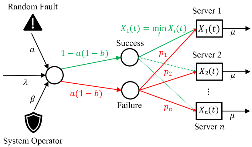
(a) Scenario of reliability failures.

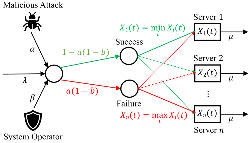
(b) Scenario of security failures.

Figure 1: An $n$-queue system with shortest-queue routing under reliability/security failures. See Section 2 for definitions of notations.

The system operator can protect/defendthe routing instructions for incoming jobs based on the state observation. The activation of protection/defense mechanisms induces a technological cost rate on the operator. For the reliability setting, we formulate the operator’s trade-off between queuing costs and protection costs as an infinite-horizon, continuous-time, and discrete-state Markov decision process. For the security setting, we formulate the interaction between the attacker and the operator as an infinite-horizon stochastic game.

To study the stability of the queuing system, previous works typically relied on characterization or approximation of the steady-state distribution of queuing states (Foley and McDonald,, 2001). However, this approach is hard to integrate with failure models. Additionally, the steady-state distribution of queuing systems with state-dependent transition rates is intricate. In response to these challenges, we adopt a Lyapunov function-based approach which has been applied to queuing systems in no-failure scenarios (Kumar and Meyn,, 1995; Dai and Meyn,, 1995; Eryilmaz and Srikant,, 2007; Xie and Jin,, 2022) and enables us to derive stability criterion for queuing systems under control and to obtain upper bounds for the mean number of jobs in the system (Meyn and Tweedie,, 1993).

To analyze the cost efficiency of the system operator’s decision, we formulate the optimization problem in terms of queuing and protection costs and then derive its Hamiltonian-Jacobian-Bellman (HJB) equation (Yong and Zhou,, 1999). We show that the optimal protecting policy under reliability failures is a deterministic threshold policy: the operator either protects or does not protect, according to threshold functions in the multi-dimensional state space. Similar approaches have been discussed in (Bertsekas,, 2012; Hajek,, 1984) for two queues, and we generalize the analysis to $n$ queues and to failure-prone settings. For the attacker-defender game, we again use HJB equation to show the threshold properties of the Markov perfect equilibria.

The above analysis leads to useful insights for designing strategic protection/defense that are both stabilizing and cost-efficient. A key finding is that the system operator has a higher incentive to protect/defend if the queues are more “imbalanced”. In addition, our numerical analysis shows that 1) the incentive to protect increases with the failure probability, decreases with the technological cost, and increases with the utilization ratio; 2) the optimal protecting policy performs better than static policies such as never protect and always protect. We also note that the optimal decision is not always stabilizing. Considering this, we propose how to compute the stability-constrained optimal policy by imposing the stability condition on the HJB equation.

Our contributions lie in the following three aspects:

• Modeling: 1) We build a framework for modeling the cyber-physical vulnerabilities of queuing systems with feedback control (dynamic routing) subject to reliability/security failures. 2) We propose a formulation of protection under reliability failures as an infinite-horizon Markov decision process and defense against security failures as an attacker-defender stochastic game.

• Analysis: 1) We provide stability criteria under failures and control based on Lyapunov functions. 2) We show the threshold properties of the optimal protection and the game equilibria on multidimensional state space based on HJB equations.

• Design: Our theoretical results provide insights on the design of traffic-stabilizing and cost-efficient protecting policy and defending response. We also propose approximate dynamic programming algorithms to numerically compute the optimal policy and equilibrium strategies.

The rest of this paper is organized as follows. Section 2 introduces the queuing model and the failure models. Section 3 studies protection against reliability failures and Section 4 analyzes defense against security failures. Section 5 gives a concluding remark.

2 Parallel servers and failure models

2.1 Parallel server system

Consider a queuing system with $n$ identical servers in parallel. Jobs (e.g., vehicles, customers, production units) arrive according to a Poisson process of rate $\lambda>0$. Each server serves jobs at an exponential rate of $\mu>0$. We use $X(t)=\begin{bmatrix}X_{1}(t)&X_{2}(t)&\cdots&X_{n}(t)\end{bmatrix}^{T}$ to denote the number of jobs at time $t$, either waiting or being served, in the $n$ servers, respectively. The state space of the parallel queuing system is $\mathbb{Z}_{\geq 0}^{n}$. Specifically, the initial system state (queue length) is $X(0)=x=[x_{1}\ x_{2}\ \cdots x_{n}]^{T}$.

We use $x+(-)e_{i}$ to denote adding 1 to (subtracting 1 from) $x_{i}$. Since the queue lengths are always non-negative, i.e. $x_{i}\geq 0$, we use $(x-e_{i})^{+}=\max(x-e_{i},0)$ to avoid the case that subtracting 1 makes the element negative. Let $x_{\min}=\min_{i}x_{i}$ and $x_{\max}=\max_{i}x_{i}$. We use $x_{-i}$ to denote variables in $x$ other than $x_{i}$, and we use the notation $x+e_{\min}$ when adding $1$ to $x_{\min}$ while keeping $x_{-i}$ the same. We call $x$ a diagonal vector if $x_{1}=x_{2}=\cdots=x_{n}$ and a non-diagonal vector otherwise. Denote the one-norm of the vector $x$ as $||x||_{1}:=x_{1}+x_{2}+\cdots+x_{n}$. Then $||X(t)||_{1}$ means the total number of jobs in the system at time $t$. We use $x\succ\boldsymbol{0}$ to denote that $x$ is not a zero vector, i.e., $||x||_{1}>0$.

Without any failures, any incoming job is allocated to the shortest queue. If there are multiple shortest queues, then the job is randomly allocated to one of them with (not necessarily equal) probabilities.

2.2 Reliability failures

Suppose that upon the arrival of a job to the system, a fault may occur with a constant probability denoted by $a\in(0,1]$. In the absence of any protection mechanism, the fault would lead to a faulty routing instruction. Consequently, the job joins a random queue with respective probabilities$p_{1},p_{2},\cdots,p_{n}\in[0,1]$, where $\sum_{i=1}^{n}p_{i}=1$. For convenience, we define

$$p_{\max}:=\max(p_{1},p_{2},\cdots,p_{n}).$$

The system operator can decide whether to protect an arriving job to ensure its optimal routing, i.e., the shortest-queue routing, as illustrated in Fig. 1(a). However, such protection comes at the cost of a rate $c_{b}>0$.

In this scenario, the system operator faces a trade-off between the queuing cost and the protection cost. We formulate this problem as an infinite-horizon continuous-time Markov decision process with the queue lengths as the states. The system operator adopts a Markovian policy denoted by $\beta:\mathbb{Z}_{\geq 0}^{n}\to\Delta(\{\text{NP},\text{P}\})$ where $\Delta(\{\text{NP},\text{P}\}):=\{(1-b,b):b\in[0,1]\}$ represents the probability distribution over the action set {not protect, protect}. The state-dependent protecting probability at state $x\in\mathbb{Z}_{\geq 0}^{n}$ is denoted as $b(x):=\beta(\text{P}\mid x)$. For simplicity, when the policy is deterministic, we write the mapping as $\beta:\mathbb{Z}_{\geq 0}^{n}\to\{\text{NP},\text{P}\}$. The state-transition matrix $P_{\mathrm{R}}:\mathbb{Z}_{\geq 0}^{n}\times\{\mathrm{NP},\mathrm{P}\}\mapsto\Delta\left(\mathbb{Z}_{\geq 0}^{n}\right)$ that captures the queuing dynamics under the protection against reliability failures is given by $P_{\mathrm{R}}(x+e_{\min}\mid x,\mathsf{b})=\left(1-a\mathbbm{1}\{\mathsf{b}=\text{NP}\}\right)\lambda$, $P_{\mathrm{R}}(x+e_{i}\mid x,\mathsf{b})=a\mathbbm{1}\{\mathsf{b}\neq\text{NP}\}p_{i}\lambda$, and $P_{\mathrm{R}}((x-e_{i})^{+}\mid x,\cdot)=\mu$, $\forall i\in[n]$, where $\mathsf{b}$ is the action chosen by the system operator at state $x$.

Formally, the objective of the system operator is to find an optimal policy $\beta$ that minimizes the expected cumulative discounted cost $J(x;\beta)$ given initial state $X(0)=x$:

$$J^{*}(x):= \min_{\beta}J(x;\beta)$$

$$=\min_{\beta} \ \mathbb{E}\Big{[}\int_{0}^{\infty}e^{-\gamma t}C(X(t),\ B(t))dt\Big{|}X(0)=x,B(t)$$

$$\sim\beta (X(t)),\ X(t+dt)\sim P_{\mathrm{R}}(\cdot\mid X(t),B(t))\Big{]},$$ (1)

where $\gamma\in(0,1)$ is the discounted factor, $B(t)\in\{\mathrm{NP},\mathrm{P}\}$ denotes the action chosen by the operator at time $t$, and $C:\mathbb{Z}_{\geq 0}^{n}\times\{\mathrm{NP},\mathrm{P}\}\to\mathbb{R}_{\geq 0}$ is the net cost rate defined as

$$C(\xi,\mathsf{b}):=||\xi||_{1}+c_{b}\mathbbm{1}\{\mathsf{b}=\text{P}\}.$$

Definition 1 (Optimal protecting policy)

The optimal protecting policy $\beta^{*}$ against reliability failures is defined as:

$$\beta^{*}(x):=\operatorname*{argmin}_{\beta}J(x;\beta),\quad\forall x\in\mathbb{Z}_{\geq 0}^{n}.$$

2.3 Security failures

Suppose that when each job arrives, a malicious attacker is able to manipulate the routing such that the job is allocated to a non-shortest queue. For ease of presentation, we consider the attacker’s best action (and thus the operator’s worst case); i.e., the job goes to the longest queue, as shown in Fig. 1(b). Let $\Delta(\{\text{NA},\text{A}\}):=\{(1-a,a):a\in[0,1]\}$ denote the probability distribution over the action set {not attack, attack}. The attacker selects a (possibly mixed) Markov strategy $\alpha:\mathbb{Z}_{\geq 0}^{n}\to\Delta(\{\text{NA},\text{A}\})$. With a slight abuse of notation, we write $a(x):=\alpha(\text{A}\mid x)$ as the state-dependent attacking probability. Note that here $a(x)$ has a different meaning from the constant fault probability $a$ in the reliability failure setting. The technological cost rate of attacking a job is $c_{a}>0$.

The system operator’s action is similar to that in the reliability setting. The only difference is that in the security setting, the system operator knows there is a strategic attacker making decisions simultaneously. We formulate the interaction between the attacker and the operator (also called defender) as an infinite-horizon stochastic game with Markov strategies that do not depend on the history of states and actions. The attacker aims to maximize the expected cumulative discounted reward $V(x;\alpha,\beta)$ given the operator’s Markov strategy $\beta$:

$$V_{A}^{*}(x;\beta):=\max_{\alpha} V(x;\alpha,\beta)]$$

$$=\max_{\alpha} \mathbb{E}\Big{[}\int_{0}^{\infty}e^{-\gamma t}R(X(t),A(t),B(t))dt\Big{|}X(0)=x,A(t)\sim\alpha(X(t)),$$

$$B(t)\sim\beta(X(t)),X(t+dt)\sim P_{\mathrm{S}}(\cdot\mid X(t),A(t),B(t))\Big{]},$$

where $A(t)\in\{\mathrm{NA},\mathrm{A}\}$ and $B(t)\in\{\mathrm{NP},\mathrm{P}\}$ denote the actions chosen by the attacker and the operator respectively at time $t$, $P_{\mathrm{S}}:\mathbb{Z}_{\geq 0}^{n}\times\{\mathrm{NA},\mathrm{A}\}\times\{\mathrm{NP},\mathrm{P}\}\mapsto\Delta\left(\mathbb{Z}_{\geq 0}^{n}\right)$ represents the transition matrix that captures the queuing dynamics under security failures, as defined by $P_{\mathrm{S}}(\xi+e_{\max}\mid\xi,\mathsf{a},\mathsf{b})=\mathbbm{1}\{\mathsf{a}=\text{A}\}\mathbbm{1}\{\mathsf{b}=\text{NP}\}\lambda$, $P_{\mathrm{S}}(\xi+e_{\min}\mid\xi,\mathsf{a},\mathsf{b})=\mathbbm{1}\{\mathsf{a}\neq\text{A}\}\mathbbm{1}\{\mathsf{b}\neq\text{NP}\}\lambda$, $P_{\mathrm{S}}((\xi-e_{i})^{+}\mid\xi,\cdot,\cdot)=\mu$, $\forall i\in[n]$, and $R:\mathbb{Z}_{\geq 0}^{n}\times\{\mathrm{NA},\mathrm{A}\}\times\{\mathrm{NP},\mathrm{P}\}\to\mathbb{R}$ is the net reward rate defined as

$$R(\xi,\mathsf{a},\mathsf{b}):=||\xi||_{1}+c_{b}\mathbbm{1}\{\mathsf{b}=\text{P}\}-c_{a}\mathbbm{1}\{\mathsf{a}=\text{A}\}.$$

Here we model the attacker-defender game as a zero-sum game, which aligns with established security game literature (Alpcan and Başar,, 2010). The attacker’s reward comprises queuing attacking costs, along with a deduction for defending costs. This is motivated by the attacker potential interest in maximizing the operator’s total operating cost, akin to competitive motives in business contests. Similarly, the operator aims to minimize the expected cumulative discounted loss given the attacker’s Markov strategy $\alpha$:

$$V_{B}^{*}(x;\alpha):=\min_{\beta}V(x;\alpha,\beta).$$

We can also define the Markov perfect equilibrium of such an attacker-defender game:

Definition 2 (Markov perfect equilibrium)

The equilibrium attacking (resp. defending) strategy $\alpha^{*}$ (resp. $\beta^{*}$) satisfies that for each state $x\in\mathbb{Z}_{\geq 0}^{n}$,

$$\alpha^{*}(x)=\operatorname*{argmax}_{\alpha}V(x;\alpha,\beta^{*})=\operatorname*{argmax}_{\alpha}V_{A}^{*}(x;\beta^{*}),$$

$$\beta^{*}(x)=\operatorname*{argmin}_{\beta}V(x;\alpha^{*},\beta)=\operatorname*{argmin}_{\beta}V_{B}^{*}(x;\alpha^{*}).$$

The equilibrium value of the attacker (defender) is $V_{A}^{*}(x;\beta^{*})$ (resp. $V_{B}^{*}(x;\alpha^{*})$). In particular, $(\alpha^{*},\beta^{*})$ is a Markov perfect equilibrium.

3 Protection against reliability failures

In this section, we consider the design of the system operator’s state-dependent protecting policy from two aspects: stability and optimality.

It is well known that a parallel $n$-server system is stabilizable if and only if the demand is less than the total capacity, i.e., $\lambda<n\mu$. In the following results, we will see that even this condition is met, in the absence of defense, reliability failures can still destabilize the queuing system, especially when the probability of failures is high and when the random faulty routing is highly heterogeneous; the following summarizes the above insights.

Proposition 1

The unprotected $n$-server system with faulty probability $a$ is stable if and only if

$$\lambda<n\mu,$$ (2a)

$$ap_{max}\lambda<\mu.$$ (2b)

Furthermore, when the system is stable, the long-time average number of jobs is upper-bounded by

$$\bar{X}:=\limsup\limits_{t\to\infty}\frac{1}{t}\int\limits_{\tau=0}^{t}\mathbb{E}[X(\tau)]d\tau\leq\frac{\lambda+n\mu}{2\left(\mu-\max(ap_{\max},\frac{1}{n})\lambda\right)}.$$

The next result provides a stability criterion for an $n$-server system with a given protecting policy. The proof of this result is presented in Section 3.1.

Theorem 1 (Stability under reliability failures)

Consider an $n$-server system with reliability failure probability $a>0$. Suppose the operator selects a Markovian policy $\beta:\mathbb{Z}_{\geq 0}^{n}\to\Delta(\{\mathrm{NP},\mathrm{P}\})$ with protection probability $b(x):=\beta(\mathrm{P}\mid x)\in[0,1]$ at state $x\in\mathbb{Z}_{\geq 0}^{n}$. Then we have the following:

1. The system is stable if for every non-diagonal vector $x$, the protecting probability $b(x)$ satisfies

   $$b(x)>1-\frac{\mu||x||_{1}-\lambda x_{\min}}{a\lambda\left(\sum\limits_{i=1}^{n}p_{i}x_{i}-x_{\min}\right)}.$$ (3)

2. When (2a) holds, there must exist a policy satisfying (3). When (2a)-(2b) hold, every policy satisfies (3).

3. If (3) holds, the long-time average number of jobs in the system is upper-bounded by

   $$\bar{X}\leq\frac{\lambda+n\mu}{2c},$$ (4)

where

$$c=\min\limits_{x\succ\boldsymbol{0}}\Big{\{}\mu-\lambda\frac{x_{\min}}{||x||_{1}}-a(1-b(x))\lambda\frac{\sum_{i=1}^{n}p_{i}x_{i}-x_{\min}}{||x||_{1}}\Big{\}}.$$

The next result implies a key finding: protection should be activated when queue lengths are more “imbalanced”.

Theorem 2 (Optimal protecting policy)

Consider an $n$-server system subject to reliability failures. An optimal deterministic protecting policy $\beta^{*}$ exists. This deterministic policy is also a threshold policy characterized by $n$ threshold functions $f_{m}$ ($m=1,2,\cdots,n$) via

$$b^{*}(x)=\mathbbm{1}\left\{\bigwedge\limits_{m=1}^{n}(f_{m}(x)>0)\right\},$$

where for each $m=1,2,\cdots,n$,

1. threshold function $f_{m}:\mathbb{Z}_{\geq 0}^{n}\to\mathbb{R}$ separates the polyhedron $\mathscr{X}_{m}=\{x\in\mathbb{Z}_{\geq 0}^{n}\mid x_{i}\geq x_{m},\ \forall 1\leq i\leq n\}$ into two subsets: $\{x\in\mathscr{X}_{m}\mid\beta^{*}(x)=\text{NP}\}$ and $\{x\in\mathscr{X}_{m}\mid\beta^{*}(x)=\text{P}\}$ by means of

   $$b^{*}(x)=\mathbbm{1}\{f_{m}(x)>0\},\quad\forall x\in\mathscr{X}_{m};$$

2. in the polyhedron $\mathscr{X}_{m}=\{x\in\mathbb{Z}_{\geq 0}^{n}\mid x_{i}\geq x_{m},\ \forall 1\leq i\leq n\}$, the optimal protecting probability $b^{*}(x)$ is monotonically non-decreasing (resp. non-increasing) in $x_{i}$ ($\forall i\neq m$) (resp. $x_{m}$) while other variables $x_{-i}$ (resp. $x_{-m}$) are fixed.

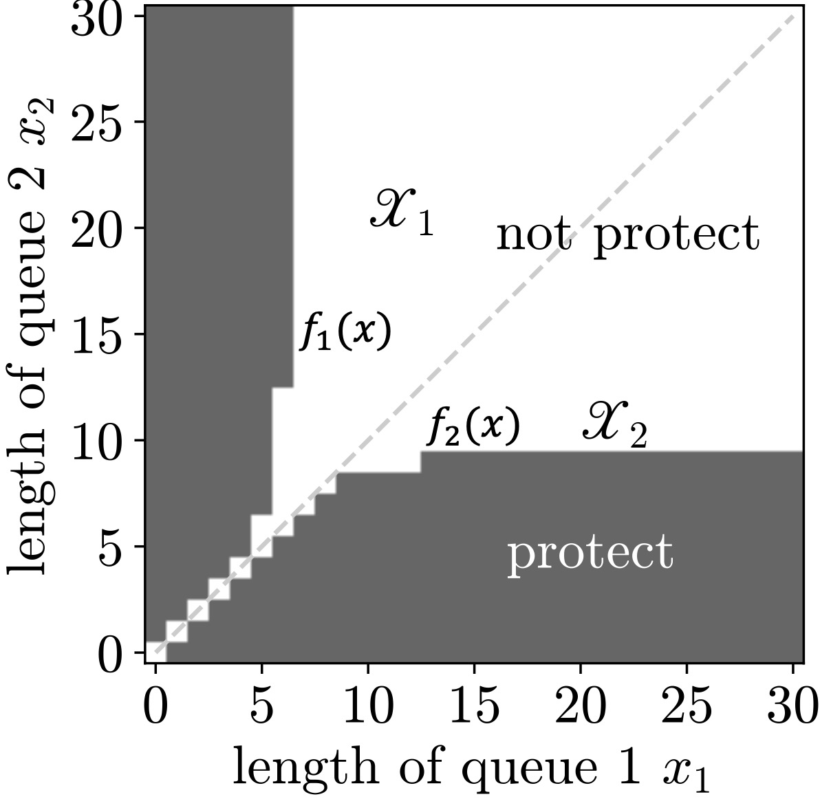
Figure 2: The characterization of the optimal protecting policy $\beta^{*}$ for a two-queue system ($p_{1}=0.1$, $p_{2}=0.9$, $\rho=0.5$, $a=0.9$).

Here (ii) supplements (i), demonstrating that the threshold functions characterize the degree of “imbalancedness”. They partition the state space into $n+1$ subsets: one “inner subset” with “balanced” states corresponding to action “not protect”, and the other $n$ “outer subsets” with “imbalanced” states for action “protect”. See the white and black areas in Fig. 2. The concept “threshold function” has appeared in prior works (Bertsekas,, 2012; Hajek,, 1984; Stidham and Weber,, 1993).

The rest of this section is devoted to the proofs and discussions of Theorem 1-2.

3.1 Stability under reliability failures

In this subsection, we provide a proof of the stability condition under the protected case (Theorem 1) and leave the proof of the stability condition under the unprotected case (Proposition 1) to Appendix A.1. Both proofs use the following theorem (Meyn and Tweedie,, 1993, Theorem 4.3):

Foster-Lyapunov drift criterion: Consider a countable-state continuous-time Markov chain $X$ with state space $S$. Let $W:S\to\mathbb{R}_{\geq 0}$ be a qualified Lyapunov function, and let $\mathcal{L}$ denote the infinitesimal generator for $W$, with the drift $\mathcal{L}W$ given by

$$\mathcal{L}W(x):=\lim\limits_{t\to 0}\frac{1}{t}\mathbb{E}[W(X(t))\mid X(0)=x]-W(x).$$

For a non-negative function $f:S\to\mathbb{R}_{\geq 0}$, if there exists $c>0$ and $d<\infty$ and a compact set $C\subset S$ such that for every $x\notin C$, the following drift condition holds:

$$\mathcal{L}W(x)\leq-cf(x)+d,$$

then for any initial condition $X(0)=x\in S$, we have

$$\limsup\limits_{t\to\infty}\frac{1}{t}\int\limits_{\tau=0}^{t}\mathbb{E}[f(X(\tau))]d\tau\leq d/c.$$

In this paper, we care about mean boundedness, i.e., the upper bound of the long-time average number of jobs. Thus, we consider the quadratic Lyapunov function

$$W(x)=\frac{1}{2}\sum_{i=1}^{n}x_{i}^{2},$$ (5)

and $f(x)=||x||_{1}$ when applying this theorem in the proofs.

Proof of Theorem 1. (i) By applying the infinitesimal generator $\mathcal{L}^{\alpha,\beta}$ to the MDP $\{X(t)\}_{t\geq 0}$ under the attacking strategy $\alpha$ and the defending strategy $\beta$ as well as the Lyapunov function (5), we have

$$\mathcal{L}^{\beta}W(x)= a(1-b(x))\lambda\sum\limits_{i=1}^{n}p_{i}\left(W(x+e_{i})-W(x)\right)$$

$$+\left(1-a(1-b(x))\right)\lambda\left(W(x+e_{\min})-W(x)\right)$$

$$+\mu\sum\limits_{i=1}^{n}\mathbbm{1}\{x_{i}>0\}\left(W(x-e_{i})-W(x)\right)$$

$$= a(1-b(x))\frac{\lambda}{2}\sum\limits_{i=1}^{n}p_{i}\left((x_{i}+1)^{2}-x_{i}^{2}\right)$$

$$+\left(1-a(1-b(x))\right)\frac{\lambda}{2}\left((x_{\min}+1)^{2}-x_{\min}^{2}\right)$$

$$+\frac{\mu}{2}\sum\limits_{i=1}^{n}\mathbbm{1}\{x_{i}>0\}\left((x_{i}-1)^{2}-x_{i}^{2}\right)$$

$$=a (1-b(x))\lambda\sum_{i=1}^{n}p_{i}x_{i}+\left(1-a(1-b(x))\right)\lambda x_{\min}$$

$$-\mu\sum_{i=1}^{n}x_{i}+\frac{1}{2}\lambda+\frac{1}{2}\sum_{i=1}^{n}\mathbbm{1}\{x_{i}>0\}\mu$$

$$\leq a (1-b(x))\lambda\left(\sum_{i=1}^{n}p_{i}x_{i}-x_{\min}\right)+(\lambda x_{\min}$$

$$-\mu||x||_{1})+\frac{1}{2}(\lambda+n\mu).$$

By (3) there exists constants $c=\min\limits_{x\succ\boldsymbol{0}}\left\{\mu-\lambda\frac{x_{\min}}{||x||_{1}}-a(1-b(x))\lambda\frac{\sum_{i=1}^{n}p_{i}x_{i}-x_{\min}}{||x||_{1}}\right\}>0$ and $d=\frac{1}{2}(\lambda+n\mu)$ such that

$$\mathcal{L}^{\beta}W(x)\leq-c||x||_{1}+d,\quad\forall x\in\mathbb{Z}_{\geq 0}^{n}.$$ (6)

(ii) When $\lambda<n\mu$, for every non-diagonal vector $x$, we have $\mu||x||_{1}-\lambda x_{\min}>\mu||x||_{1}-\lambda\frac{||x||_{1}}{n}=\left(\mu-\frac{\lambda}{n}\right)||x||_{1}>0$ and $\sum_{i=1}^{n}p_{i}x_{i}-x_{\min}>0$, then

$$1-\frac{\mu||x||_{1}-\lambda x_{\min}}{a\lambda\left(\sum\limits_{i=1}^{n}p_{i}x_{i}-x_{\min}\right)}<1.$$

Thus, $b(x)\equiv 1$ satisfies the stability condition (3) and $\beta(x)\equiv\text{P}$ is a stabilizing policy that exists.

When $\max(ap_{\max},1/n)\lambda<\mu$, for every non-diagonal vector $x$, we have $a\lambda\sum_{i=1}^{n}p_{i}x_{i}+(1-a)\lambda x_{\min}\leq\max(ap_{\max},1/n)\lambda||x||_{1}<\mu||x||_{1}$, and then

$$1-\frac{\mu||x||_{1}-\lambda x_{\min}}{a\lambda\left(\sum\limits_{i=1}^{n}p_{i}x_{i}-x_{\min}\right)}<0.$$

Thus, every policy satisfies the stability criterion (3).

By (Meyn and Tweedie,, 1993, Theorem 4.3), this drift condition implies the upper bound (4) and thus the stability. $\square$

Theorem 1 provides a stability criterion for any state-dependent protecting probability. This implies that the operator needs to protect, i.e., choose some positive protecting probability to stabilize the system at certain states (queue lengths). We will use such stabilizing threshold probabilities to obtain a stability-constrained optimal policy. See Section 3.3 and Appendix A.4.

3.2 Optimal protecting policy

A standard way to solve the discounted infinite-horizon minimization problem (1) is to write down its HJB equation for optimality (Chang,, 2004, Chapter 4):

$$0=\min\limits_{\beta}\{||x||_{1}+c_{b}b(x)-\gamma J^{*}(x)+\mathcal{L}^{\beta}J^{*}(x)\}.$$ (7)

We can rewrite it as the following recurrence form:

$$(\gamma+\lambda+n\mu)J^{*}(x)= \min\limits_{\beta}\Bigg{\{}||x||_{1}+c_{b}b(x)+\mu\sum\limits_{i=1}^{n}J^{*}((x-e_{i})^{+})+\lambda J^{*}(x+e_{\min})$$

$$+(1-b(x))a\lambda\bigg{(}\sum\limits_{i=1}^{n}p_{i}J^{*}(x+e_{j})-J^{*}(x+e_{\min})\bigg{)}\Bigg{\}}.$$ (8)

The optimal protecting policy $\beta^{*}$ is essentially the solution of (7) and (8). By a standard result of discrete-state finite-action MDP (Puterman,, 2014, Theorem 6.2.10), an optimal deterministic stationary policy exists. Furthermore, in the no-failure scenario ($a=0$), the operator never needs to protect (i.e., $\forall x$, $\beta^{*}(x)=\text{NP}$); and when all queue lengths are equal, i.e., $x_{1}=x_{2}=\cdots=x_{n}$, the operator deterministically deactivates the protection.

Proof of Theorem 2(i). The expression to be minimized in the right-hand side of the HJB equation (8) is linear in $b(x)$, so the minimum is reached at the endpoints, that is, $b(x)=0$ or $b(x)=1$. $\square$

Now the HJB equation (8) turns into

$$(\gamma+\lambda+n\mu)J^{*}(x)= \min\limits_{b\in\{0,1\}}\Big{\{}||x||_{1}+c_{b}b+\mu\sum\limits_{i=1}^{n}J^{*}((x-e_{i})^{+})+\lambda J^{*}(x+e_{\min})$$

$$+(1-b)a\lambda\Big{(}\sum\limits_{i=1}^{n}p_{i}J^{*}(x+e_{i})-J^{*}(x+e_{\min})\Big{)}\Big{\}}.$$

Let $\tilde{\lambda}=\lambda/(\gamma+\lambda+n\mu)$, $\tilde{\mu}=\mu/(\gamma+\lambda+n\mu)$, and $\tilde{J}^{*}(\cdot)=(\gamma+\lambda+n\mu)J^{*}(\cdot)$, then we have

$$\tilde{J}^{*}(x)= \min\limits_{b\in\{0,1\}}\Big{\{}||x||_{1}+c_{b}b+\tilde{\mu}\sum\limits_{i=1}^{n}\tilde{J}^{*}((x-e_{i})^{+})+\tilde{\lambda}\tilde{J}^{*}(x+e_{\min})$$

$$+(1-b)a\tilde{\lambda}\Big{(}\sum\limits_{i=1}^{n}p_{i}\tilde{J}^{*}(x+e_{i})-\tilde{J}^{*}(x+e_{\min})\Big{)}\Big{\}}.$$ (9)

Proof of Theorem 2(ii). By applying the DP recursion technique (Bertsekas,, 2012, Chapter 4.6), we can demonstrate (a) the existence of the threshold functions by showing (b) the monotonicity of the optimal protecting probability: $\forall x\in\mathbb{Z}_{\geq 0}^{n}$, let $m=\operatorname*{argmin}_{i}x_{i}$, then

$$\begin{split}&b^{*}(x+e_{i})\geq b^{*}(x),\quad\forall i\neq m\\ &b^{*}(x-e_{m})\geq b^{*}(x).\end{split}$$ (10)

Now we prove (10). Let $\Delta^{*}(x)=\sum\limits_{i=1}^{n}p_{i}\tilde{J}^{*}(x+e_{i})-\tilde{J}^{*}(x+e_{m})$. Note that by Definition 1 and Theorem 2(i), $b^{*}(x)=1$ if $\Delta^{*}(x)>c_{b}/(a\tilde{\lambda})$ and $b^{*}(x)=0$ if $\Delta^{*}(x)<c_{b}/(a\tilde{\lambda})$. Then the monotonicity of $b^{*}$ is essentially the monotonicity of $\Delta^{*}$. Thus, (10) is equivalent to

$$\begin{split}&\Delta^{*}(x+e_{i})\geq\Delta^{*}(x),\quad\forall i\neq m\\ &\Delta^{*}(x-e_{m})\geq\Delta^{*}(x).\end{split}$$ (11)

We defer the proof of (11) to Appendix A.2. The high-level idea is to use induction based on value iteration. $\square$

To obtain an estimated optimal policy, we propose an algorithm called truncated policy iteration (TPI). See Algorithm 1 in Appendix A.4. It is adapted from the classic policy iteration algorithm (Sutton and Barto,, 2018) and based on the following value iteration form of the HJB equation (3.2):

$$\tilde{J}^{k+1}(x)= \min\limits_{b\in\{0,1\}}\Big{\{}||x||_{1}+c_{b}b+\tilde{\mu}\sum\limits_{i=1}^{n}\tilde{J}^{k}((x-e_{i})^{+})+\tilde{\lambda}\tilde{J}^{k}(x+e_{\min})$$

$$+(1-b)a\tilde{\lambda}\Big{(}\sum\limits_{i=1}^{n}p_{i}\tilde{J}^{k}(x+e_{i})-\tilde{J}^{k}(x+e_{\min})\Big{)}\Big{\}}$$ (12)

Now we can use the estimated optimal policy to conduct numerical analysis on 1) the relationship between the incentive to protect and the system parameters; 2) the comparison between the optimal policy and two naive static policies: always protect and never protects.

We first analyze the tipping points when the system operator starts to protect “riskier” states under the optimal policy $\beta^{*}$, i.e., $\exists x$ s.t. $\beta^{*}(x)=\text{P}$, as the failure probability $a$ and technological cost $c_{b}$ change. It can be seen from Fig. 3 that the incentive to protect is non-decreasing in the failure probability $a$, non-increasing in the technological cost $c_{b}$ and non-decreasing in the utilization ratio (a.k.a. traffic-intensity and demand-capacity ratio) $\rho=\lambda/(n\mu)$. That is, the system operator has higher incentive to protect when 1) the failure probability is higher; 2) the technological cost is lower; 3) the utilization ratio is higher.

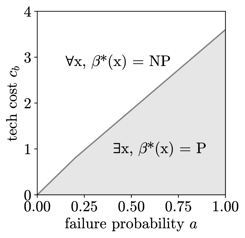
(a) $\rho=0.8$

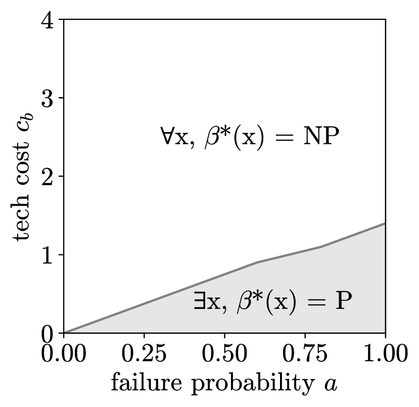
(b) $\rho=0.2$

Figure 3: The tipping points when the system operator starts to protect “riskier” states under the optimal policy as the failure probability and the technological cost change.

In the following simulation, we will see that the optimal policy $\beta^{*}$ can significantly reduce the security risk, compared to the static policies: $\beta(x)\equiv\text{P}$ (always protects) and $\beta(x)\equiv\text{NP}$ (never protects). See Fig. 4 where the yellow curves are below the red curves and the green curves. The Monte Carlo simulation result is based on the cumulative discounted cost within 50000s. Here the cumulative discounted cost is calculated as the sum of the total queuing cost and total technological cost in the episode, and we normalized it to be a value between 0 and 1. Note that under the static policy $\beta(x)\equiv\text{P}$ (i.e., $\forall x$, $b(x)=1$), the job always joins the shortest queue regardless of the failure probability, so the cumulative discounted cost is a constant (red curve).

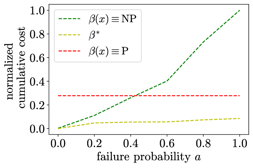
(a) $c_{b}=0.05$

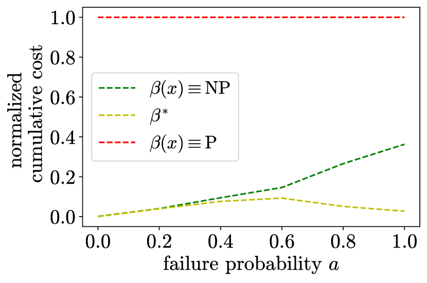
(b) $c_{b}=0.5$

Figure 4: Comparison of the normalized cumulative discounted costs between the optimal policy and the static policies ($p_{1}=0.1$, $p_{2}=0.9$, $\rho=0.8$).

3.3 Stability-constrained optimal policy

The optimal policy may not always be stabilizing. For example, the optimal policy under the system parameters $p_{1}=0.1$, $p_{2}=0.9$, $\rho=0.5$, $a=0.9$ does not satisfy the stability condition (3). To address this issue, we can select an optimal policy satisfying the stability condition (3) by solving a stability-constrained MDP (Zanon et al.,, 2022). This involves adding an additional constraint (3) to the optimal control problem (1). We call the solution stability-constrained optimal policy and denote it as $\hat{\beta}^{*}$. This policy, unlike the optimal one, involves randomization over actions {P, NP} at some states, see Fig. 5. Appendix A.4 gives a corresponding modification of the TPI algorithm.

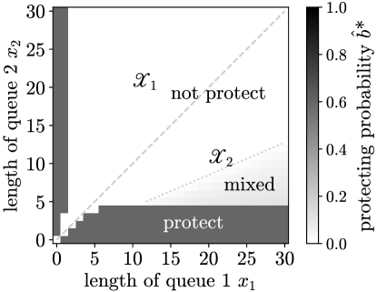
Figure 5: The characterization of the stability-constrained optimal policy $\hat{\beta}^{*}$ for a two-queue system ($p_{1}=0.1$, $p_{2}=0.9$, $\rho=0.5$, $a=0.9$).

Additionally, we can have a quick check of the existence of a stabilizing policy and stabilizability of the optimal policy using stability conditions (2a)-(2b) as follows:

• When (2a)-(2b) hold, i.e., $\max(ap_{\max},1/n)\lambda<\mu$, the optimal protecting policy is also stabilizing.

• When only (2a) holds, i.e., $\lambda/n<\mu\leq ap_{\max}\lambda$, the optimal protecting policy may not be stabilizing.

• When (2a) does not hold, i.e., $\lambda\geq\mu n$, no stabilizing protecting policy exists.

4 Defense against security failures

In this section, we analyze the attacker’s attacking strategy and system operator’s defending strategy from two aspects: stability and game equilibrium.

The following criterion can be used for checking the stability of the $n$-server system under any state-dependent attacking and defending strategies:

Theorem 3 (Stability under security failures)

Consider an $n$-server system subject to security failures. Suppose that at each state $x\in\mathbb{Z}_{\geq 0}^{n}$, the attacker (resp. system operator) attacks (resp. defends) each job following Markov strategy $\alpha$ (resp. $\beta$) characterized by a state-dependent probability $a(x)\in[0,1]$ (resp. $b(x)\in[0,1]$). Then we have the following:

1. The system is stable if for every non-diagonal vector $x$, the attacking and defending probabilities $a(x)$ and $b(x)$ satisfy

   $$a(x)\left(1-b(x)\right)<\frac{\mu||x||_{1}-\lambda x_{\min}}{\lambda(x_{\max}-x_{\min})}.$$ (13)

2. When $\lambda<n\mu$, there must exist a strategy $\beta$ with defending probability $b(x)$ satisfying (13).

3. Furthermore, if (13) holds, then the long-time average number of jobs is upper-bounded by

   $$\bar{X}\leq\frac{\lambda+n\mu}{2c},$$ (14)

   where

   $$c=\min\limits_{x\succ\boldsymbol{0}}\Big{\{}\mu-\lambda\frac{x_{\min}}{||x||_{1}}-a(x)(1-b(x))\lambda\frac{x_{\max}-x_{\min}}{||x||_{1}}\Big{\}}.$$

The next result characterizes the structure of the strategy of the Markov perfect equilibria of the stochastic game: the equilibrium defending probability is higher when the queue lengths are more “imbalanced”.

Theorem 4 (Markov perfect equilibrium)

The Markov perfect equilibrium (MPE) of the attacker-defender stochastic game exists, and the following holds:

1. $(\alpha^{*},\beta^{*})$ is qualitatively different over the following three subsets of the state space $\mathbb{Z}_{\geq 0}^{n}$:

   1. $S_{1}=\{x\in\mathbb{Z}_{\geq 0}^{n}\mid(\alpha^{*}(x),\beta^{*}(x))=(\text{NA},\text{NP})\}$; (“low risk”)

   2. $S_{2}=\{x\in\mathbb{Z}_{\geq 0}^{n}\mid(\alpha^{*}(x),\beta^{*}(x))=(\text{A},\text{NP})\}$; (“medium risk”)

   3. $S_{3}=\{x\in\mathbb{Z}_{\geq 0}^{n}\mid(\alpha^{*}(x),\beta^{*}(x))\text{ is mixed}\}$. (“high risk”)

2. The boundaries between $S_{1}$ and $S_{2}$, as well as those between $S_{2}$ and $S_{3}$ are characterized by threshold functions $g_{ij},h_{ij}$ ($1\leq i\neq j\leq n$) as follows:

   $$S_{1}=\left\{x\in\mathbb{Z}_{\geq 0}^{n}\mid\bigwedge\limits_{1\leq i\neq j\leq n}(g_{ij}(x)<0)\right\},$$

   $$S_{2}=\left\{x\in\mathbb{Z}_{\geq 0}^{n}\mid\bigwedge\limits_{1\leq i\neq j\leq n}(g_{ij}(x)>0\vee h_{ij}(x)<0)\right\},$$

   $$S_{3}=\left\{x\in\mathbb{Z}_{\geq 0}^{n}\mid\bigwedge\limits_{1\leq i\neq j\leq n}(h_{ij}(x)>0)\right\}.$$

   where for each $i,j=1,2,\cdots,n$ ($i\neq j$),

   1. $g_{ij},h_{ij}:\mathbb{Z}_{\geq 0}^{n}\to\mathbb{R}$ separate the polyhedron $\mathscr{X}_{ij}=\{x\in\mathbb{Z}_{\geq 0}^{n}\mid x_{i}=x_{\max},\ x_{j}=x_{\min}\}$ into three subsets: $S_{1}\cap\mathscr{X}_{ij}$, $S_{2}\cap\mathscr{X}_{ij}$ and $S_{3}\cap\mathscr{X}_{ij}$;

   2. state $x$ has a lower (resp. higher) or equal security level than state $x+e_{i}$ (resp. $x+e_{j}$).

The threshold functions here also characterize the degree of “unbalancedness”. Intuitively, $S_{1}$–$S_{3}$ correspond to various security risk levels, and thus correspond to the incentive of the operator to defend: when the queues are more “unbalanced”, the security risk is higher, and the system operator has a higher incentive to defend. Fig. 6 visualizes the equilibria for a two-queue system, which help understand Theorem 4. For a detailed argument about the relationship between the security levels and system parameters (e.g., technological costs and utilization ratio), see Section 4.2.

Figure 6: The equilibrium attacking and defending strategies for a two-queue system ($\rho=0.5$, $c_{a}=0.1$, $c_{b}=0.2$).

We also find that the security game has four equilibrium regimes under different combinations of attack cost $c_{a}$ and defense cost $c_{b}$; see Fig. 7. Each regime is labeled with corresponding subsets of Markov perfect equilibria and security levels.

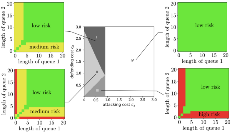
Figure 7: Equilibrium regimes of the security game ($\rho=0.8$).

The rest of this section is devoted to the proofs of Theorem 3-4, as well as an additional discussion on Markov perfect equilibrium.

4.1 Stability under security failures

Proof of Theorem 3. (i) By applying infinitesimal generator $\mathcal{L}^{\alpha,\beta}$ under the attacking strategy $\alpha$ and the defending strategy $\beta$ to the same Lyapunov function (5), we have

$$\mathcal{L}^{\alpha,\beta}W(x):= \lim\limits_{t\to 0}\frac{1}{t}\mathbb{E}[W(X(t))\mid X(0)=x;\alpha,\beta]-W(x)$$

$$= a(x)(1-b(x))\lambda\left(W(x+e_{\max})-W(x)\right)$$

$$+\left(1-a(x)(1-b(x))\right)\lambda\left(W(x+e_{\min})-W(x)\right)$$

$$+\mu\sum\limits_{i=1}^{n}\mathbbm{1}\{x_{i}>0\}\left(W(x-e_{i})-W(x)\right)$$

$$= a(x)(1-b(x))\frac{\lambda}{2}\left((x_{\max}+1)^{2}-x_{i}^{2}\right)$$

$$+\left(1-a(x)(1-b(x))\right)\frac{\lambda}{2}\left((x_{\min}+1)^{2}-x_{\min}^{2}\right)$$

$$+\frac{\mu}{2}\sum\limits_{i=1}^{n}\mathbbm{1}\{x_{i}>0\}\left((x_{i}-1)^{2}-x_{i}^{2}\right)$$

$$= a(x)(1-b(x))\lambda x_{\max}+\left(1-a(x)(1-b(x))\right)$$

$$\lambda x_{\min}-\sum_{i=1}^{n}\mu x_{i}+\frac{1}{2}\lambda+\frac{1}{2}\sum_{i=1}^{n}\mathbbm{1}\{x_{i}>0\}\mu$$

$$\leq a(x)(1-b(x))\lambda(x_{\max}-x_{\min})$$

$$+\lambda x_{\min}-\mu||x||_{1}+\frac{1}{2}(\lambda+n\mu).$$ (15)

Hence, by (13) there exists $c=\min\limits_{x\succ\boldsymbol{0}}\{\mu-\lambda\frac{x_{\min}}{||x||_{1}}-a(x)(1-b(x))\lambda\frac{x_{\max}-x_{\min}}{||x||_{1}})\}>0$ and $d=\frac{1}{2}(\lambda+n\mu)$ such that

$$\mathcal{L}^{\alpha,\beta}W(x)\leq-c||x||_{1}+d,\quad\forall x\in\mathbb{Z}_{\geq 0}^{n}.$$

(ii) When $\lambda<n\mu$, for every non-diagonal vector $x$, we have $\mu||x||_{1}\geq n\mu x_{\min}>\lambda x_{\min}$, and $x_{\max}>x_{\min}$, implying $\frac{\mu||x||_{1}-\lambda x_{\min}}{\lambda(x_{\max}-x_{\min})}>0$. Thus, no matter what strategy the attacker chooses, the defending strategy with $b(x)\equiv 1$ satisfies the stability condition (13).

(iii) By (Meyn and Tweedie,, 1993, Theorem 4.3), the drift condition (15) implies the upper bound (14) and thus the stability. $\square$

4.2 Markov perfect equilibrium

For the attacker-defender stochastic game, we first show the existence of Markov perfect equilibrium.

Proposition 2

Markov perfect equilibrium $(\alpha^{*},\beta^{*})$ of the stochastic attacker-defender game always exists.

Proof. Note that the state space $\mathbb{Z}_{\geq 0}^{n}$ is countable and the action space $\{0,1\}$ is finite (and thus compact). By (Federgruen,, 1978, Theorem 1), Markov perfect equilibrium (also called discounted equilibrium point of policies) exists. $\square$

Next, we discuss the derivation of Markov perfect equilibria. According to Shapley’s extension on minimax theorem for stochastic game (Shapley,, 1953), the attacker and the defender have the same equilibrium (minimax) value:

$$V_{B}^{*}(x;\alpha^{*})=V_{A}^{*}(x;\beta^{*})=V^{*}(x).$$

Thus, we only need to compute the minimax value $V^{*}$ of the stochastic game. Similar to the derivation of (3.2), we obtain the following HJB equation of the minimax problem (letting $\tilde{V}^{*}(\cdot)=(\rho+\lambda+n\mu)V^{*}(\cdot)$):

$$\tilde{V}^{*}(x)= \max_{\alpha}\min_{\beta}\bigg{\{}||x||_{1}+c_{b}b(x)-c_{a}a(x)+\tilde{\mu}\sum\limits_{i}\tilde{V}^{*}((x-e_{i})^{+})$$

$$+\tilde{\lambda}\tilde{V}^{*}(x+e_{\min})+a(x)(1-b(x))\tilde{\lambda}\Big{(}\tilde{V}^{*}(x+e_{\max})-\tilde{V}^{*}(x+e_{\min})\Big{)}\bigg{\}}.$$ (16)

For each state $x\in\mathbb{Z}_{\geq 0}^{n}$, let $\delta^{*}(x)=\tilde{\lambda}(\tilde{V}^{*}(x+e_{\max})-\tilde{V}^{*}(x+e_{\min}))$ and build an auxiliary matrix game

$$M(x,\tilde{V}^{*})= \Big{(}||x||_{1}+\tilde{\mu}\sum\limits_{i=1}^{n}\tilde{V}^{*}((x-e_{i})^{+})+\tilde{\lambda}\tilde{V}^{*}(x+e_{\min})\Big{)}$$

$$\begin{bmatrix}1&1\\ 1&1\end{bmatrix}+\begin{bmatrix}0&c_{b}\\ -c_{a}+\delta^{*}(x)&-c_{a}+c_{b}\end{bmatrix}.$$ (17)

Then given $\delta^{*}(x)$, the equilibrium strategies $(\alpha^{*}(x),\beta^{*}(x))$ can be obtained by Shapley-Snow method (Shapley and Snow,, 1952), a convenient algorithm for finding the minimax value and equilibrium strategies of any two-player zero-sum game.

Proof of Theorem 4(i). Consider the matrix game $M(x,\tilde{V}^{*})$ defined as (17) where the attacker and the system operator are the row player and the column player. Based on Shapley-Snow method, the equilibrium strategies $(\alpha^{*}(x),\beta^{*}(x))$ are in the following three cases depending on the relationship between $\delta^{*}(x)$ and the technological costs $c_{a},c_{b}>0$:

1. When $\delta^{*}(x)\leq c_{a}$, it is obvious that $\alpha^{*}(x)=\text{NA}$ (i.e., $a^{*}(x)=0$) is a dominant strategy. Then $c_{b}>0$ implies $\beta^{*}(x)=\text{NP}$ (i.e., $b^{*}(x)=0$). That is, the attacker has no incentive to attack, and thus the defender does not need to defend. At this pure strategy equilibrium, the security risk is low.

2. When the defense cost $c_{b}$ is higher then the attack cost $c_{a}$, and $c_{a}<\delta^{*}(x)\leq c_{b}$, it is obvious that $\beta^{*}(x)=\text{NP}$ (i.e., $b^{*}(x)=0$) is a dominant strategy. Then $c_{b}>-c_{a}+c_{b}$ implies $\alpha^{*}(x)=\text{A}$ (i.e., $a^{*}(x)=1$). That is, the defender has no incentive to defend and consequently the attacker prefers to attack. At this pure strategy equilibrium, the security risk is higher than the first case but tolerable.

3. When $\delta^{*}(x)>\max\{c_{a},c_{b}\}>0$, no saddle point exists. Then both the attacker and the system operator consider mixed strategies such that $a^{*}(x)=\frac{c_{b}}{\delta^{*}(x)}$, $b^{*}(x)=1-\frac{c_{a}}{\delta^{*}(x)}$. Particularly, the operator needs to select positive protecting probability, and now the security risk is high.

The above three cases correspond to the three subsets of states. Note that the subset $S_{2}$ is empty when $c_{a}>c_{b}$. $\square$

From the above proof, we observe that for fixed technological costs $c_{a}$ and $c_{b}$, the security risk level is only higher when $\delta^{*}$ is larger. Then as in the proof of Theorem 2, we use the fact that the monotonicity of the security risk level is equivalent to the monotonicity of $\delta^{*}$ to show the threshold property of the equilibrium. Now we are ready to present the proof of Theorem 4(ii) which uses symmetry (property (i)) and Schur Convexity (property (ii)).

Proof of Theorem 4(ii). For any $x\in\mathbb{Z}_{\geq 0}^{n}$, let $l=\operatorname*{argmax}_{i}x_{i},\ m=\operatorname*{argmin}_{i}x_{i}$. Then $\delta^{*}(x)=\tilde{\lambda}(\tilde{V}^{*}(x+e_{l})-\tilde{V}^{*}(x+e_{m}))$. Since the monotonicity of the security risk level of the states is equivalent to the monotonicity of $\delta^{*}$, and implies the existence of the threshold functions, it is sufficient to show that $\delta^{*}$ is monotonically non-decreasing (resp. non-increasing) in the largest variable (resp. the smallest variable) when other variables are fixed; that is,

$$\delta^{*}(x+e_{l})\geq\delta^{*}(x),\quad\delta^{*}(x-e_{m})\geq\delta^{*}(x).$$ (18)

The proof of (18) also uses induction based on value iteration and can be found in Appendix A.3. $\square$

4.3 Equilibrium computation and equilibrium regimes

First, we discuss the numerical computation of the minimax value $V^{*}(x)$ and the equilibrium strategies $(\alpha^{*}(x),\beta^{*}(x))$ for each state $x$. Based on the value iteration form of HJB equation (4.2), we develop an algorithm adapted from Shapley’s algorithm (Shapley,, 1953; Alpcan and Başar,, 2010; Thai et al.,, 2016). See Algorithm 2 in Appendix 2.

The algorithm proceeds as follows. Initialize $\tilde{V}^{0}(x)$. In each iteration $k$ and for each state $x$, let $\delta^{k}(x)=\tilde{\lambda}(\tilde{V}^{k}(x+e_{\max})-\tilde{V}^{k}(x+e_{\min}))$ and build an auxiliary matrix game $M(x,\tilde{V}^{k})$ similar to (17); then update $\tilde{V}^{k+1}(x)$ with the minimax value $val(M)$ given by Shapley-Snow method:

• when $\delta^{k}(x)\leq c_{a}$, $val(M)=||x||_{1}+\tilde{\mu}\sum\limits_{i=1}^{n}\tilde{V}^{k}((x-e_{i})^{+})+\tilde{\lambda}\tilde{V}^{k}(x+e_{\min})$;

• when $c_{a}<\delta^{k}(x)\leq c_{b}$, $val(M)=||x||_{1}-c_{a}+\tilde{\mu}\sum\limits_{i=1}^{n}\tilde{V}^{k}((x-e_{i})^{+})+\tilde{\lambda}\tilde{V}^{k}(x+e_{\max})$;

• when $\delta^{k}(x)>\max\{c_{a},c_{b}\}$, $val(M)=||x||_{1}+c_{b}+\tilde{\mu}\sum\limits_{i=1}^{n}\tilde{V}^{k}((x-e_{i})^{+})+\tilde{\lambda}\tilde{V}^{k}(x+e_{\min})-\frac{c_{a}c_{b}}{\delta^{k}(x)}$.

When $\tilde{V}^{k}(x)$ converges to $\tilde{V}^{*}(x)$, we again use Shapley-Snow method to solve the matrix game $M(x,\tilde{V}^{*})$ and obtain the estimation of the equilibrium $(\alpha^{*}(x),\beta^{*}(x))$.

Next, we discuss the existence of different security levels under different combinations of $c_{a}$ and $c_{b}$. We have seen that no medium risk state exists when $c_{a}>c_{b}$.

In Fig. 7, various regimes correspond to particular combinations of security levels. Under large attack cost, the attacker has no incentive to attack, then only the low risk states exist (see regime IV). When the attack cost goes smaller but still greater than the defense cost ($c_{a}>c_{b}$), not only the low risk states but also the high risk states exist (see regime III) since the attacker has less incentive to attack. As the defense cost increases to be greater than the attack cost ($c_{b}>c_{a}$), the defender has less incentive to defend, and now all risk levels including the medium risk exist (see regime II).

Last, we remark that deriving a stability-constrained equilibrium is not reasonable as stability constraints can only be imposed on the system operator, not the attacker. Nevertheless, we can derive stability-constrained best responses for the operator based on (13), given the attacker’s strategy.

5 Concluding Remarks

In this work, we address the reliability and security concerns of service systems with dynamic routing and propose cost-efficient protection/defense advice for system operators. Moreover, our theoretical results can provide insights for real-world applications like vehicle navigation, signal-free intersection control, flight dispatch, and data packet routing. Interesting future directions include 1) detailed analysis of stability-constrained optimal policies/best responses; 2) extension to general queuing networks, note that stability for renewal arrival processes and general service times can be readily established using fluid model techniques (Dai and Meyn,, 1995); 3) design of practical near-optimal heuristic policies and analysis of optimality gaps; and 4) design of efficient (in both time and space) computational algorithms that mitigate the curse of dimensionality in scenarios involving numerous parallel servers.

Appendix A Appendices

A.1 Proof of Proposition  1

Here we provide the proof of the stability condition for unprotected system using standard results on Poisson process subdivision and the stability of generalized join the shortest queue systems (Foley and McDonald,, 2001, Theorem 1).

Stability of generalized JSQ: Let $N=\{1,2,\cdots,n\}$ be the set of $n$ exponential servers. For each nonempty subset $S\subset N$, define the traffic intensity on $S$ as

$$\rho_{S}:=\frac{\sum_{S^{\prime}\subset S}\lambda_{S^{\prime}}}{\mu_{S}}=\frac{\sum_{S^{\prime}\subset S}\lambda_{S^{\prime}}}{\sum_{i\in S}\mu_{i}}.$$

Let $\rho_{\max}:=\max_{S\subset N}\rho_{S}$ be the traffic intensity of the most heavily loaded subset. The generalized join the shortest queue system is stable if and only if $\rho_{\max}<1$.

Proof of proposition 1. The unprotected $n$-queue system has $n+1$ classes of jobs. The $i$-th class enters server $i$ as a Poisson process of rate $ap_{i}\lambda$ ($1\leq i\leq n$). The $(n+1)$-th class enters the $n$-queue system as a Poisson process of rate $(1-a)\lambda$; when a job of this class arrives, the job joins the shortest queue. By (Foley and McDonald,, 2001, Theorem 1), the $(n+1)$-class, $n$-queue system is stable if and only if

$$\rho_{S}:=\frac{\sum_{S^{\prime}\subset S}\lambda_{S^{\prime}}}{\mu_{S}}=\frac{\sum_{S^{\prime}\subset S}\lambda_{S^{\prime}}}{\sum_{i\in S}\mu_{i}}.$$

which is equivalent to (2a)-(2b).

Consider the same quadratic Lyapunov function (5) and apply the infinitesimal generator, we have

$$\mathcal{L}W(x):= \lim\limits_{t\to 0}\frac{1}{t}\mathbb{E}[W(X(t))\mid X(0)=x]-W(x)$$

$$= a(1-b)\lambda\sum\limits_{i=1}^{n}p_{i}\left(W(x+e_{i})-W(x)\right)$$

$$+\left(1-a(1-b\right)\lambda\left(W(x+e_{\min})-W(x)\right)$$

$$+\mu\sum\limits_{i=1}^{n}\mathbbm{1}\{x_{i}>0\}\left(W(x-e_{i})-W(x)\right)$$

$$= a\frac{\lambda}{2}\sum\limits_{i=1}^{n}p_{i}\left((x_{i}+1)^{2}-x_{i}^{2}\right)$$

$$+(1-a)\frac{\lambda}{2}\left((x_{\min}+1)^{2}-x_{\min}^{2}\right)$$

$$+\frac{\mu}{2}\sum\limits_{i=1}^{n}\mathbbm{1}\{x_{i}>0\}\left((x_{i}-1)^{2}-x_{i}^{2}\right)$$

$$= a\lambda\sum_{i=1}^{n}p_{i}x_{i}+(1-a)\lambda x_{\min}-\mu\sum_{i=1}^{n}x_{i}+\frac{\lambda}{2}+\frac{\mu}{2}\sum_{i=1}^{n}\mathbbm{1}\{x_{i}>0\}$$

$$\leq \left(\max(ap_{\max},1/n)\lambda-\mu\right)||x||_{1}+\frac{1}{2}(\lambda+n\mu).$$

Hence, by (2a)–(2b) there exists a constant $c=\mu-\max(ap_{\max},1/n)\lambda>0$ and $d=\frac{1}{2}(\lambda+n\mu)$ such that

$$\mathcal{L}W(x)\leq-c||x||_{1}+d,\quad\forall x\in\mathbb{Z}_{\geq 0}^{n}.$$

By (Meyn and Tweedie,, 1993, Theorem 4.3), this drift condition implies the upper bound and thus the stability. $\square$

A.2 Induction part of Theorem 2

In this subsection, we continue the proof of Theorem 2 with the induction proving (11).

Let $\Delta^{k}(x)=\sum\limits_{i=1}^{n}p_{i}\tilde{J}^{k}(x+e_{i})-\tilde{J}^{k}(x+e_{m})$, it is sufficient to show for all $k\in\mathbb{N}$,

$$\begin{split}\Delta^{k}(x+e_{i})&\geq\Delta^{k}(x),\quad\forall i\neq m\\ \Delta^{k}(x-e_{m})&\geq\Delta^{k}(x).\end{split}$$

One can verify that the above hold for $k=0,1,2$ with the fact that $\tilde{J}^{0}=0$, $\tilde{J}^{1}(x)=||x||_{1}$ and $\tilde{J}^{2}(x)=(1++n\mu)||x||_{1}+-\mu\sum_{i}\mathbbm{1}\{x_{i}>0\}$. Here we consider multiple base cases to avoid reaching trivial conclusions, say all inequalities are just equalities.

Now we show the inductive step. According to the value iteration (3.2), we have $\forall j\neq m$,

$$\Delta^{k+1}(x+e_{j})-\Delta^{k+1}(x)$$

$$= \mu\sum_{i=1}^{n}[\Delta^{k}((x+e_{j}-e_{i})^{+})-\Delta^{k}((x-e_{i})^{+})]$$ (19)

$$+[\Delta^{k}(x+e_{j}+e_{m})-\Delta^{k}(x+e_{m})]$$ (20)

$$+f^{k}(x+e_{j})-f^{k}(x),$$ (21)

$$\Delta^{k+1}(x-e_{m})-\Delta^{k+1}(x)$$

$$= \tilde{\mu}\sum_{i=1}^{n}[\Delta^{k}((x-e_{m}-e_{i})^{+})-\Delta^{k}((x-e_{i})^{+})]$$ (22)

$$+[\Delta^{k}(x)-\Delta^{k}(x+e_{m})]$$ (23)

$$+f^{k}(x-e_{m})-f^{k}(x),$$ (24)

where $f^{k}(x):=\sum_{i=1}^{n}p_{i}\min\Big{\{}c_{b},a\Delta^{k}(x+e_{i})\Big{\}}-\min\Big{\{}c_{b},a\Delta^{k}(x+e_{m})\Big{\}}$.

Note that based on the induction hypothesis, we have $\forall j\neq m$,

$$\Delta^{k}((x+e_{j}-e_{i})^{+}) \geq\Delta^{k}((x-e_{i})^{+}),$$ (25)

$$\Delta^{k}(x+e_{j}+e_{m}) \geq\Delta^{k}(x+e_{m}),$$ (26)

$$\Delta^{k}(x+e_{j}+e_{i}) \geq\Delta^{k}(x+e_{i}),$$ (27)

$$\Delta^{k}((x-e_{m}-e_{i})^{+}) \geq\Delta^{k}((x-e_{i})^{+}),$$ (28)

$$\Delta^{k}(x) \geq\Delta^{k}(x+e_{m}),$$ (29)

$$\Delta^{k}(x-e_{m}+e_{i}) \geq\Delta^{k}(x+e_{i}).$$ (30)

Then (25) and (28) naturally lead to $\eqref{eq_inductive1}\geq 0$ and $\eqref{eq_inductive4}\geq 0$ respectively. We can also use (26)-(27) to discuss the possibilities of (21) under the min operations and derive $\eqref{eq_inductive2}+\eqref{eq_inductive3}\geq 0$. For example, when $\Delta^{k}(x+e_{j}+e_{i})\geq\Delta^{k}(x+e_{i})\geq\frac{c_{b}}{a}$ and $\Delta^{k}(x+e_{j}+e_{m})\geq\Delta^{k}(x+e_{m})\geq\frac{c_{b}}{a}$, we have $\eqref{eq_inductive2}+\eqref{eq_inductive3}=a\sum_{i=1}^{n}p_{i}\left(\Delta^{k}(x+e_{j}+e_{i})-\Delta^{k}(x+e_{i})\right)+(1-a)\left(\Delta^{k}(x+e_{j}+e_{m})-\Delta^{k}(x+e_{m})\right)\geq 0$. Similarly, we can obtain $\eqref{eq_inductive5}+\eqref{eq_inductive6}\geq 0$ using (29)-(30).

Thus, we can conclude that $\eqref{eq_inductive1}+\eqref{eq_inductive2}+\eqref{eq_inductive3}\geq 0$ and $\eqref{eq_inductive4}+\eqref{eq_inductive5}+\eqref{eq_inductive6}\geq 0$, which yield

$$\Delta^{k+1}(x+e_{j})\geq\Delta^{k+1}(x),\quad\forall j\neq m,$$

$$\Delta^{k+1}(x-e_{m})\geq\Delta^{k+1}(x).$$

A.3 Induction part of Theorem 4

In this subsection, we continue the proof of Theorem 4 with the induction proving (18).

Let $\delta^{k}(x)=\tilde{\lambda}(\tilde{V}^{k}(x+e_{l})-\tilde{V}^{k}(x+e_{m}))$, it is sufficient to show for all $k\in\mathbb{N}$,

$$\delta^{k}(x+e_{l})\geq\delta^{k}(x),\quad\delta^{k}(x-e_{m})\geq\delta^{k}(x).$$

For the base cases, one can verify that the above inequalities hold for $k=0,1,2$. Now we show the inductive step. According to the value iteration form of formula (4.2),

$$\delta^{k+1}(x+e_{l})-\delta^{k+1}(x)$$

$$= \tilde{\mu}[\delta^{k}(x)-\delta^{k}((x-e_{l})^{+})]$$

$$+ \tilde{\mu}[\delta^{k}((x+e_{l}-e_{m})^{+})-\delta^{k}((x-e_{m})^{+})]$$

$$+ \tilde{\lambda}[\delta^{k}(x+e_{l}+e_{m})-\delta^{k}(x+e_{m})]$$

$$+ g^{k}(x+2e_{l})-g^{k}(x+e_{l}+e_{m})-g^{k}(x+e_{l})+g^{k}(x+e_{m}),$$

where

$$g^{k}(x)=\max\Big{\{}0,\min\Big{\{}\delta^{k}(x)-c_{a},c_{b}-\frac{c_{a}c_{b}}{\delta^{k}(x)}\Big{\}}\Big{\}}.$$

Note that based on the induction hypothesis, we have

$$\delta^{k}((x+e_{l}-e_{m})^{+})\geq\delta^{k}((x-e_{m})^{+})\geq\delta^{k}(x)\geq\delta^{k}((x-e_{l})^{+}),$$

$$\delta^{k}(x+2e_{l})\geq\delta^{k}(x+e_{l})\geq\delta^{k}(x+e_{l}+e_{m})\geq\delta^{k}(x+e_{m}).$$

Then we can conclude that $\delta^{k+1}(x+e_{l})\geq\delta^{k+1}(x)$ and prove $\delta^{k+1}(x-e_{m})\geq\delta^{k+1}(x)$ in a similar way.

A.4 Truncated policy iteration

In this subsection, we present the truncated policy iteration algorithm for estimating stability-constrained optimal policy. This algorithm is adapted from the classic policy iteration algorithm (Sutton and Barto,, 2018) by combining the stability condition (3). Since the original state space is countably infinite, here we set a boundary to make the state space finite so that the algorithm can terminate in finite steps.

Algorithm 1 Truncated policy iteration for estimating optimal policy $\beta\approx\beta^{*}$ (continuing)

Algorithm parameter: small $\epsilon>0$ 
Input: arrival rate $\lambda$, service rate $\mu$, discounted factor $\rho$, number of queues $n$, unit protection cost $c_{b}$, probabilities of joining queues $p_{1},p_{2},\cdots,p_{n}$ 
Initialize arrays: $J(x)\in\mathbb{R}$ and $b(x)\in\{0,1\}$ arbitrarily (e.g., $J(x)=0$, $b(x)=0$) for all $x\in\mathcal{X}=\{0,1,\cdots,B\}^{n}$  # $B$ is the queue length upper bound

$\tilde{\lambda}\leftarrow\lambda/(\rho+\lambda+n\mu),\quad\tilde{\mu}\leftarrow\mu/(\rho+\lambda+n\mu)$
repeat

       repeat

             $\Delta\leftarrow 0$ # Policy evaluation
foreach $x\in\mathcal{X}$ do

                   $v\leftarrow J(x)$
$J(x)\leftarrow\min\limits_{b\in\{0,1\}}\bigg{\{}||x||_{1}+c_{b}b+\tilde{\mu}\sum\limits_{i=1}^{n}J((x-e_{i})^{+})+\tilde{\lambda}J(x+e_{\min})+(1-b)a\tilde{\lambda}\bigg{[}\sum\limits_{i=1}^{n}p_{i}J(x+e_{i})-J(x+e_{\min})\bigg{]}\bigg{\}}$
$\Delta\leftarrow\max(\Delta,|v-J(x)|)$

             end foreach

            

      until $|v-V(x)|<\epsilon$;

      $stable\leftarrow True$ # Policy improvement
foreach $x\in\mathcal{X}$ do

             old-action$\leftarrow b(x)$
if $a\tilde{\lambda}\left(\sum\limits_{i}p_{i}J(x+e_{i})-J(x+e_{\min})\right)\leq c_{b}$ then

                   $b(x)=0$

             end if

            else

                   $b(x)=1$

             end if

            if old-action$\neq b(x)$ then

                   $stable\leftarrow False$

             end if

            

       end foreach

      

until $stable=True$;

Output $\beta=(1-b)\text{NP}+b\text{P}\approx\beta^{*}$

A.5 Adapted Shapley’s algorithm

Here we present the adapted Shapley’s algorithm for computing the minimax value and equilibrium strategies of the attacker-defender stochastic game. In each iteration, it builds an auxiliary matrix game and obtains the minimax value using Shapley-Snow method (Shapley and Snow,, 1952).

Set $V(x)=0$ for all $x\in\mathcal{X}=\{0,1,2,\cdots,B\}^{n}$
repeat

       foreach $x\in\mathcal{X}$ do

             $v\leftarrow V(x)$
Build auxiliary matrix game $M(x,V)$
Compute the minimax value $val(M)$ by using Shapley-Snow method
$V(x)\leftarrow val(M)$

       end foreach

      

until $|v-V(x)|<\epsilon$;

foreach $x\in\mathcal{X}$ do

       Build auxiliary matrix game $M(x,V)$
Compute $\alpha$ and $\beta$ from $M(x,V)$ by using Shapley-Snow method

end foreach

Algorithm 2 Adapted Shapley’s algorithm for estimating equilibrium strategies $\beta\approx\beta^{*}$, $\alpha\approx\alpha^{*}$ (continuing)

References

- Al-Kahtani, (2012) Al-Kahtani, M. S. (2012). Survey on security attacks in vehicular ad hoc networks (vanets). In 2012 6th international conference on signal processing and communication systems, pages 1–9. IEEE.
- Alpcan and Başar, (2010) Alpcan, T. and Başar, T. (2010). Network security: A decision and game-theoretic approach. Cambridge University Press.
- Barrère et al., (2020) Barrère, M., Hankin, C., Nicolaou, N., Eliades, D. G., and Parisini, T. (2020). Measuring cyber-physical security in industrial control systems via minimum-effort attack strategies. Journal of information security and applications, 52:102471.
- Bertsekas, (2012) Bertsekas, D. (2012). Dynamic programming and optimal control, vol II: Approximate dynamic programming.
- Beutler and Teneketzis, (1989) Beutler, F. J. and Teneketzis, D. (1989). Routing in queueing networks under imperfect information: Stochastic dominance and thresholds. Stochastics: An International Journal of Probability and Stochastic Processes, 26(2):81–100.
- Bohacek et al., (2007) Bohacek, S., Hespanha, J., Lee, J., Lim, C., and Obraczka, K. (2007). Game theoretic stochastic routing for fault tolerance and security in computer networks. IEEE transactions on parallel and distributed systems, 18(9):1227–1240.
- Cardenas et al., (2009) Cardenas, A., Amin, S., Sinopoli, B., Giani, A., Perrig, A., Sastry, S., et al. (2009). Challenges for securing cyber physical systems. In Workshop on future directions in cyber-physical systems security, volume 5. Citeseer.
- Chang, (2004) Chang, F.-R. (2004). Stochastic optimization in continuous time. Cambridge University Press.
- Dai and Meyn, (1995) Dai, J. G. and Meyn, S. P. (1995). Stability and convergence of moments for multiclass queueing networks via fluid limit models. IEEE Transactions on Automatic Control, 40(11):1889–1904.
- De Persis and Tesi, (2015) De Persis, C. and Tesi, P. (2015). Input-to-state stabilizing control under denial-of-service. IEEE Transactions on Automatic Control, 60(11):2930–2944.
- Ephremides et al., (1980) Ephremides, A., Varaiya, P., and Walrand, J. (1980). A simple dynamic routing problem. IEEE transactions on Automatic Control, 25(4):690–693.
- Eryilmaz and Srikant, (2007) Eryilmaz, A. and Srikant, R. (2007). Fair resource allocation in wireless networks using queue-length-based scheduling and congestion control. IEEE/ACM Transactions on Networking (TON), 15(6):1333–1344.
- Eschenfeldt and Gamarnik, (2018) Eschenfeldt, P. and Gamarnik, D. (2018). Join the shortest queue with many servers. the heavy-traffic asymptotics. Mathematics of Operations Research, 43(3):867–886.
- Federgruen, (1978) Federgruen, A. (1978). On n-person stochastic games by denumerable state space. Advances in Applied Probability, 10(2):452–471.
- Feng et al., (2022) Feng, Y., Huang, S. E., Wong, W., Chen, Q. A., Mao, Z. M., and Liu, H. X. (2022). On the cybersecurity of traffic signal control system with connected vehicles. IEEE Transactions on Intelligent Transportation Systems.
- Foley and McDonald, (2001) Foley, R. D. and McDonald, D. R. (2001). Join the shortest queue: stability and exact asymptotics. The Annals of Applied Probability, 11(3):569–607.
- Fraile et al., (2018) Fraile, F., Tagawa, T., Poler, R., and Ortiz, A. (2018). Trustworthy industrial iot gateways for interoperability platforms and ecosystems. IEEE Internet of Things Journal, 5(6):4506–4514.
- Gravé-Lazi, (2014) Gravé-Lazi, L. (2014). Technion students find way to hack waze, create fake traffic jams. The Jerusalem Post Available at: https://www.jpost.com/enviro-tech/technion-students-find-way-to-hack-waze-create-fake-traffic-jams-346377.
- Gupta et al., (2007) Gupta, V., Balter, M. H., Sigman, K., and Whitt, W. (2007). Analysis of join-the-shortest-queue routing for web server farms. Performance Evaluation, 64(9-12):1062–1081.
- Hajek, (1984) Hajek, B. (1984). Optimal control of two interacting service stations. IEEE transactions on automatic control, 29(6):491–499.
- Halfin, (1985) Halfin, S. (1985). The shortest queue problem. Journal of Applied Probability, 22(4):865–878.
- Iravani et al., (2011) Iravani, S. M., Kolfal, B., and Van Oyen, M. P. (2011). Capability flexibility: a decision support methodology for parallel service and manufacturing systems with flexible servers. IIE Transactions, 43(5):363–382.
- Jin and Amin, (2018) Jin, L. and Amin, S. (2018). Stability of fluid queueing systems with parallel servers and stochastic capacities. IEEE Transactions on Automatic Control, 63(11):3948–3955.
- Knessl et al., (1986) Knessl, C., Matkowsky, B., Schuss, Z., and Tier, C. (1986). Two parallel queues with dynamic routing. IEEE transactions on communications, 34(12):1170–1175.
- Kumar and Meyn, (1995) Kumar, P. and Meyn, S. P. (1995). Stability of queueing networks and scheduling policies. IEEE Transactions on Automatic Control, 40(2):251–260.
- Kuri and Kumar, (1995) Kuri, J. and Kumar, A. (1995). Optimal control of arrivals to queues with delayed queue length information. IEEE Transactions on Automatic Control, 40(8):1444–1450.
- Laszka et al., (2019) Laszka, A., Abbas, W., Vorobeychik, Y., and Koutsoukos, X. (2019). Detection and mitigation of attacks on transportation networks as a multi-stage security game. Computers & Security, 87:101576.
- Manshaei et al., (2013) Manshaei, M. H., Zhu, Q., Alpcan, T., Bacşar, T., and Hubaux, J.-P. (2013). Game theory meets network security and privacy. ACM Computing Surveys (CSUR), 45(3):25.
- Mehdian et al., (2017) Mehdian, S., Zhou, Z., and Bambos, N. (2017). Join-the-shortest-queue scheduling with delay. In 2017 American Control Conference (ACC), pages 1747–1752. IEEE.
- Meyn and Tweedie, (1993) Meyn, S. P. and Tweedie, R. L. (1993). Stability of markovian processes iii: Foster–lyapunov criteria for continuous-time processes. Advances in Applied Probability, 25(3):518–548.
- Neely et al., (2001) Neely, M., Modiano, E., and Rohrs, C. (2001). Packet routing over parallel time-varying queues with application to satellite and wireless networks. In PROCEEDINGS OF THE ANNUAL ALLERTON CONFERENCE ON COMMUNICATION CONTROL AND COMPUTING, volume 39, pages 1110–1111. The University; 1998.
- Ouyang and Teneketzis, (2015) Ouyang, Y. and Teneketzis, D. (2015). Signaling for decentralized routing in a queueing network. Annals of Operations Research, pages 1–39.
- Puterman, (2014) Puterman, M. L. (2014). Markov decision processes: discrete stochastic dynamic programming. John Wiley & Sons.
- Sakiz and Sen, (2017) Sakiz, F. and Sen, S. (2017). A survey of attacks and detection mechanisms on intelligent transportation systems: Vanets and iov. Ad Hoc Networks, 61:33–50.
- Shapley, (1953) Shapley, L. S. (1953). Stochastic games. Proceedings of the national academy of sciences, 39(10):1095–1100.
- Shapley and Snow, (1952) Shapley, L. S. and Snow, R. (1952). Basic solutions of discrete games. Contributions to the Theory of Games, 1:27–35.
- Stidham and Weber, (1993) Stidham, S. and Weber, R. (1993). A survey of markov decision models for control of networks of queues. Queueing systems, 13(1):291–314.
- Sutton and Barto, (2018) Sutton, R. S. and Barto, A. G. (2018). Reinforcement learning: An introduction. MIT press.
- Tang et al., (2020) Tang, Y., Wen, Y., and Jin, L. (2020). Security risk analysis of the shorter-queue routing policy for two symmetric servers. In 2020 American Control Conference (ACC), pages 5090–5095. IEEE.
- Thai et al., (2016) Thai, J., Yuan, C., and Bayen, A. M. (2016). Resiliency of mobility-as-a-service systems to denial-of-service attacks. IEEE Transactions on Control of Network Systems, 5(1):370–382.
- Wang et al., (2007) Wang, Y., Lin, C., Li, Q.-L., and Fang, Y. (2007). A queueing analysis for the denial of service (dos) attacks in computer networks. Computer Networks, 51(12):3564–3573.
- Xie and Jin, (2022) Xie, Q. and Jin, L. (2022). Stabilizing queuing networks with model data-independent control. IEEE Transactions on Control of Network Systems.
- Yong and Zhou, (1999) Yong, J. and Zhou, X. Y. (1999). Stochastic controls: Hamiltonian systems and HJB equations, volume 43. Springer Science & Business Media.
- Zanon et al., (2022) Zanon, M., Gros, S., and Palladino, M. (2022). Stability-constrained markov decision processes using mpc. Automatica, 143:110399.