Direct Parameterization of Lipschitz-Bounded Deep Networks

Abstract

This paper introduces a new parameterization of deep neural networks (both fully-connected and convolutional) with guaranteed $\ell^{2}$ Lipschitz bounds, i.e. limited sensitivity to input perturbations. The Lipschitz guarantees are equivalent to the tightest-known bounds based on certification via a semidefinite program (SDP). We provide a “direct” parameterization, i.e., a smooth mapping from $\mathbb{R}^{N}$ onto the set of weights satisfying the SDP-based bound. Moreover, our parameterization is complete, i.e. a neural network satisfies the SDP bound if and only if it can be represented via our parameterization. This enables training using standard gradient methods, without any inner approximation or computationally intensive tasks (e.g. projections or barrier terms) for the SDP constraint. The new parameterization can equivalently be thought of as either a new layer type (the sandwich layer), or a novel parameterization of standard feedforward networks with parameter sharing between neighbouring layers. A comprehensive set of experiments on image classification shows that sandwich layers outperform previous approaches on both empirical and certified robust accuracy. Code is available at https://github.com/acfr/LBDN.

1 Introduction

Neural networks have enjoyed wide application due to their many favourable properties, including highly accurate fits to training data, surprising generalisation performance within a distribution, as well as scalability to very large models and data sets. Nevertheless, it has also been observed that they can be highly sensitive to small input perturbations (Szegedy et al., 2014). This is a critical limitation in applications in which certifiable robustness is required, or the smoothness of a learned function is important.

A standard way to quantify sensitivity of models is via a Lipschitz bound, which generalises the notion of a slope-restricted scalar function. A function $x\mapsto f(x)$ between normed spaces satisfies a Lipschitz bound $\gamma$ if

$$\|f(x_{1})-f(x_{2})\|\leq\gamma\|x_{1}-x_{2}\|$$ (1)

for all $x_{1},x_{2}$ in its domain. The (true) Lipschitz constant of a function, denoted by $\mathrm{Lip}(f)$, is the smallest such $\gamma$. Moreover, we call $f$ a $\gamma$-Lipschitz function if $\mathrm{Lip}(f)\leq\gamma$.

A natural application of Lipschitz-bounds is to control a model’s sensitivity to adversarial (worst-case) inputs, e.g. (Madry et al., 2018; Tsuzuku et al., 2018), but they can also be effective for regularisation (Gouk et al., 2021) and Lipschitz constants often appear in theoretical generalization bounds (Bartlett et al., 2017; Bubeck & Sellke, 2023). Lipschitz-bounded networks have found many applications, including: stabilising the learning of generative adversarial networks (Arjovsky et al., 2017; Gulrajani et al., 2017); implicit geometry mechanisms for computer graphics (Liu et al., 2022); in reinforcement learning to controlling sensitivity to measurement noise (e.g. (Russo & Proutiere, 2021)) and to ensure robust stability of feedback loops during learning (Wang & Manchester, 2022); and the training of differentially-private neural networks (Bethune et al., 2023). In robotics applications, several learning-based planning and control algorithms require known Lipschitz bounds in learned stability certificates, see e.g. the recent surveys (Brunke et al., 2022; Dawson et al., 2023).

Unfortunately, even for two-layer perceptrons with ReLU activations, exact calculation of the true Lipschitz constant for $\ell^{2}$ (Euclidean) norms is NP-hard (Virmaux & Scaman, 2018), so attention has focused on approximations that balance accuracy with computational tractability. Crude $\ell^{2}$-bounds can be found via the product of spectral norms of layer weights (Szegedy et al., 2014), however to date the most accurate polynomial-time computable bounds require solution of a semidefinite program (SDP) (Fazlyab et al., 2019), which is computationally tractable only for relatively small fully-connected networks.

While certification of a Lipschitz bound of a network is a (convex) SDP with this method, the set of weights satisfying a prescribed Lipschitz bound is non-convex, complicating training. Both (Rosca et al., 2020) and (Dawson et al., 2023) highlight the computationally-intensive nature of SDP-based bounds as limitations for applications.

Contribution.

In this paper we introduce a new parameterization of standard feedforward neural networks, both fully-connected multi-layer perceptron (MLP) and deep convolutional neural networks (CNN).

• The proposed parameterization has built-in guarantees on the network’s Lipschitz bound, equivalent to the best-known bounds provided by the SDP method (Fazlyab et al., 2019).

• Our parameterization is a smooth surjective mapping from an unconstrained parameter space $\mathbb{R}^{N}$ onto the (non-convex) set of network weights satisfying these SDP-based bounds. This enables learning of lipschitz-bounded networks via standard gradient methods, avoiding the complex projection steps or barrier function computations that have previously been required and limited scalability.

• The new parameterization can equivalently be treated as either a composition of new $1$-Lipschitz layers called Sandwich layer, or a parameterization of standard feedforward networks with coupling parameters between neighbouring layers.

Notation.

Let $\mathbb{R}$ be the set of real numbers. $A\succeq 0$ means that a square matrix $A$ is a positive semi-definite. We denote by $\mathbb{D}_{++}^{n}$ for the set of $n\times n$ positive diagonal matrices. For a vector $x\in\mathbb{R}^{n}$, its $2$-norm is denoted by $\|x\|$. Given a matrix $A\in\mathbb{R}^{m\times n}$, $\|A\|$ is defined as its the largest singular value and $A^{+}$ denotes its Moore–Penrose pseudoinverse.

2 Problem Setup and Preliminaries

Consider an $L$-layer feedforward neural network $y=f(x)$ described by the following recursive equations:

$$\begin{split}z_{0}&=x,\\ z_{k+1}&=\sigma(W_{k}z_{k}+b_{k}),\quad k=0,\ldots,L-1\\ y&=W_{L}z_{L}+b_{L},\end{split}$$ (2)

where $x\in\mathbb{R}^{n_{0}},z_{k}\in\mathbb{R}^{n_{k}},y\in\mathbb{R}^{n_{L+1}}$ are the network input, hidden unit of the $k$th layer and network output, respectively. Here $W_{k}\in\mathbb{R}^{n_{k+1}\times n_{k}}$ and $b_{k}\in\mathbb{R}^{n_{k+1}}$ are the weight matrix and bias vector for the $k$th layer, and $\sigma$ is a scalar activation function applied element-wise. We make the following assumption, which holds for most commonly-used activation functions (possibly after rescaling) (Goodfellow et al., 2016).

Assumption 2.1.

The nonlinear activation $\sigma:\mathbb{R}\rightarrow\mathbb{R}$ is piecewise differentiable and slope-restricted in $[0,1]$.

If different channels have different activation functions, then we simply require that they all satisfy the above assumption.

The main goal of this work is to learn feedforward networks (2) with certified Lipschitz bound of $\gamma$, i.e.,

$$\min_{\phi}\;\mathcal{L}(f_{\phi})\quad\mathrm{s.t.}\quad\mathrm{Lip}(f_{\phi})\leq\gamma$$ (3)

where $\mathcal{L}(\cdot)$ is a loss function and $\phi:=\{(W_{k},b_{k})\}_{0\leq k\leq L}$ is the learnable parameter. Since it is NP-hard to compute $\mathrm{Lip}(f_{\phi})$, we seek an accurate Lipschitz bound estimation so that the constraint in (3) does not lead to a significant restriction on the model expressivity.

In (Fazlyab et al., 2019), integral quadratic constraint (IQC) methods were applied to capture both monotonicity and 1-Lipschitzness properties of $\sigma$, leading to state-of-the-art Lipschitz bound estimation based on the following linear matrix inequality (LMI), see details in Appendix A:

$$H:=\begin{bmatrix}\gamma I&-U^{\top}\Lambda&0\\ -\Lambda U&2\Lambda-\Lambda W-W^{\top}\Lambda&-Y^{\top}\\ 0&-Y&\gamma I\end{bmatrix}\succeq 0$$ (4)

where $\Lambda\in\mathbb{D}_{++}^{n}$ with $n=\sum_{k=1}^{L}n_{k}$, and

$$W=\begin{bmatrix}0&&&\\ W_{1}&\ddots&&\\ \vdots&\ddots&0&\\ 0&\cdots&W_{L-1}&0\end{bmatrix},\;U=\begin{bmatrix}W_{0}\\ 0\\ \vdots\\ 0\end{bmatrix},$$

$$Y=\begin{bmatrix}0&\cdots&0&W_{L}\end{bmatrix}.$$

Remark 2.2.

The published paper (Fazlyab et al., 2019) claimed that even tighter Lipschitz bounds could be achieved with a less restrictive class of multipliers $\Lambda$ than diagonal. However, this is false: a counterexample was presented in (Pauli et al., 2021), and the error in the proof was explained in (Revay et al., 2020b), see also Remark A.2 in the appendix of this paper.

In this paper we approach problem (3) via model parameterizations guaranteeing a given Lipschitz bound.

Definition 2.3.

A parameterization of the network (2) is a differentiable mapping $\phi=\mathcal{M}(\theta)$ where $\theta\in\Theta\subseteq\mathbb{R}^{N}$. It is called a convex parameterization if $\Theta$ is convex, and a direct parameterization if $\Theta=\mathbb{R}^{N}$.

Given a network with fixed $W,U,Y$, Condition (4) is convex with respect to the Lipschitz bound $\gamma$ and multiplier $\Lambda$. When training a network with specified bound $\gamma$, we can convert (4) into a convex parameterization by introducing new decision variables $\tilde{U}=\Lambda U,\tilde{W}=\Lambda W$, (4) becomes

$$H=\begin{bmatrix}\gamma I&-\hat{W}_{0}^{\top}&\\ -\hat{W}_{0}&2\Lambda_{0}&-\hat{W}_{1}^{\top}\\ &\ddots&\ddots&\ddots\\ &&-\hat{W}_{L-1}&2\Lambda_{L-1}&-\hat{W}_{L}^{\top}\\ &&&-\hat{W}_{L}&\gamma I\end{bmatrix}\succeq 0$$ (5)

where $\hat{W}_{k}=\Lambda_{k}W_{k}$ for $0\leq k<L$ and $\hat{W}_{L}=W_{L}$. In (Pauli et al., 2021; Revay et al., 2020a), constrained optimization methods such as convex projection and barrier functions are applied for training. However, even for relatively small-scale networks (e.g. $\sim 1000$ neurons), the associated barrier terms or projections become a major computational bottleneck.

3 Direct Parameterization

In this section we will present our main contribution – a direct parameterization $\phi=\mathcal{M}(\theta)$ such that $\phi$ automatically satisfies (4) and hence (1) for any $\theta\in\mathbb{R}^{N}$. Then, the learning problem (3) can be transformed into an unconstrained optimization problem

$$\min_{\theta\in\mathbb{R}^{N}}\quad\mathcal{L}(f_{\mathcal{M}(\theta)}).$$

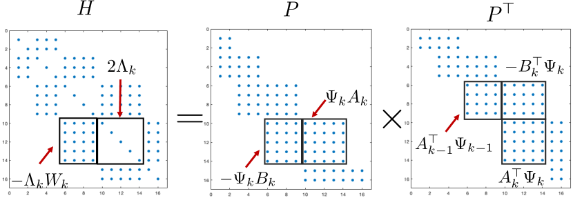
Figure 1: Illustration of the sparsity pattern in $H$ that must be preserved by the factorization $H=PP^{\top}$.

First, it is clear that (5) is satisfied if we parameterize $H$ as $H=PP^{\top}$. The main challenge then is to parameterize $P$ such that the particular sparsity pattern of $H$ is recovered: a block-tridiagonal structure where the main diagonal blocks must be positive diagonal matrices, see Equation 5 and Figure 1. First, the block-tridiagonal structure can be achieved by taking

$$P=\begin{bmatrix}D_{-1}&\\ -V_{0}&D_{0}&\\ &\ddots&\ddots&\\ &&-V_{L}&D_{L}\end{bmatrix},$$

i.e., block Cholesky factorization of $H$. The next step is to construct $V_{k}$ and $D_{k}$ such that the diagonal blocks $H_{kk}=V_{k}V_{k}^{\top}+D_{k}D_{k}^{\top}$ are diagonal matrices. We do so by the Cayley transform for orthogonal matrix parameterization (Trockman & Kolter, 2021), i.e., for any $X\in\mathbb{R}^{m\times m},Y\in\mathbb{R}^{n\times m}$ we have $Q^{\top}Q=I$ if

$$Q=\operatorname{Cayley}\left(\begin{bmatrix}X\\ Y\end{bmatrix}\right):=\begin{bmatrix}(I+Z)^{-1}(I-Z)\\ -2Y(I+Z)^{-1}\end{bmatrix}$$ (6)

with $Z=X-X^{\top}+Y^{\top}Y$. To be more specific, we take $D_{k}=\Psi_{k}A_{k}$ and $V_{k}=\Psi_{k}B_{k}$ where

$$\Psi_{k}=\operatorname{diag}\bigl{(}e^{d_{k}}\bigr{)},\quad\begin{bmatrix}A_{k}^{\top}\\ B_{k}^{\top}\end{bmatrix}=\operatorname{Cayley}\left(\begin{bmatrix}X_{k}\\ Y_{k}\end{bmatrix}\right)$$ (7)

for some free vector $d_{k}$ and matrices $X_{k},Y_{k}$ with proper dimension. Now we can verify that $H=PP^{\top}$ has the same structure as (5), i.e.,

$$H_{kk}=\Psi_{k}(A_{k}A_{k}^{\top}+B_{k}B_{k}^{\top})\Psi_{k}=\Psi_{k}^{2},$$

$$H_{k-1,k}=-\Psi_{k}B_{k}A_{k-1}^{\top}\Psi_{k-1}.$$

Moreover, we can construct the multiplier $\Lambda_{k}=\frac{1}{2}\Psi_{k}^{2}$ and the weight matrix

$$W_{k}=-\Lambda_{k}^{-1}H_{k-1,k}=2\Psi_{k}^{-1}B_{k}A_{k-1}^{\top}\Psi_{k-1}$$ (8)

with $k=0,\ldots,L$, where $A_{-1}=I,\Psi_{-1}=\sqrt{\gamma/2}I$ and $\Psi_{L}=\sqrt{2/\gamma}I$ with $\gamma$ as the prescribed Lipschitz bound.

We summarize our model parameterization as follows. The free parameter $\theta$ consists of bias terms $b_{k}\in\mathbb{R}^{n_{k+1}}$ and

$$d_{j}\in\mathbb{R}^{n_{j}},\;X_{k}\in\mathbb{R}^{n_{k+1}\times n_{k+1}},\;Y_{k}\in\mathbb{R}^{n_{k}\times n_{k+1}}$$

with $0\leq j<L$ and $0\leq k\leq L$. The weight $W_{k}$ is constructed via (7) and (8). Notice that $W_{k}$ depends on parameters of index $k$ and $k-1$, i.e. there is an “interlacing” coupling between parameters and weights, see Figure 2.

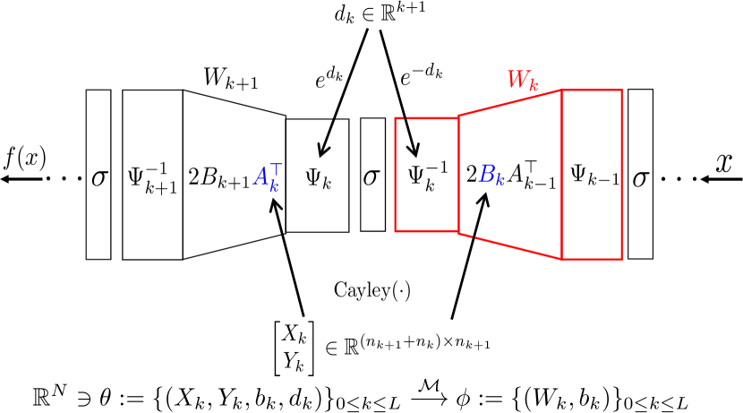
Figure 2: Direct parameterization for Lipschitz-bounded deep networks, i.e. $\mathrm{Lip}(f_{\phi})\leq\gamma$ with $\phi=\mathcal{M}(\theta)$ for all $\theta\in\mathbb{R}^{N}$. Note that free parameters are shared across neighbouring layers.

3.1 Theoretical results

The main theoretical results is that our parameterization is complete (necessary and sufficient) for the set of DNNs satisfying the LMI constraint (5) of (Fazlyab et al., 2019).

Theorem 3.1.

The feedforward network (2) satisfies the LMI condition (5) if and only if its weight matrices $W_{k}$ can be parameterized via (8).

The proof to this and all other theorems can be found in Appendix D.

1-Lipschitz sandwich layer.

Here we show that the new parameterization can also be interpreted as a new layer type. We first introduce new hidden units $h_{k}=\sqrt{2}A_{k}^{\top}\Psi_{k}z_{k}$ for $k=0,\ldots L$ and then rewrite the proposed LBDN model as

$$\begin{split}h_{0}=&\sqrt{\gamma}x\\ h_{k+1}=&\sqrt{2}A_{k}^{\top}\Psi_{k}\sigma(\sqrt{2}\Psi_{k}^{-1}B_{k}h_{k}+b_{k})\\ y=&\sqrt{\gamma}B_{L}h_{L}+b_{L}.\end{split}$$ (9)

The core component of the above model is a sandwich-structured layer of the form:

$$h_{\mathsf{out}}=\sqrt{2}A^{\top}\Psi\sigma\bigl{(}\sqrt{2}\Psi^{-1}Bh_{\mathsf{in}}+b\bigr{)}$$ (10)

where $h_{\mathsf{in}}\in\mathbb{R}^{p},h_{\mathsf{out}}\in\mathbb{R}^{q}$ are the layer input and output, respectively. Unlike the parameterization in (8), consecutive layers in (9) do not have coupled free parameters, which allows for modular implementation. Another advantage is that such representation can reveal some fundamental insights on the roles of $\Psi,A$ and $B$.

Theorem 3.2.

The layer (10) with $\Psi,A,B$ constructed by (7) is 1-Lipschitz.

To understand the role of $\Psi$, we look at a new activation layer which is obtained by placing $\Psi^{-1}\in\mathbb{D}_{++}^{q}$ and $\Psi$ before and after $\sigma$, i.e., $u=\Psi\sigma(\Psi^{-1}v+b)$. Here $\Psi$ can change the shape and shift the position of individual activation channels while keeping their slopes within $[0,1]$, allowing the optimizer to search over a rich set of activations.

For the roles of $A$ and $B$, we need to look at another special case of (10) where $\sigma$ is the identity operator. Then, (10) becomes a linear layer

$$h_{\mathsf{out}}=2A^{\top}Bh_{\mathsf{in}}+\hat{b}.$$ (11)

As a direct corollary of Theorem 3.2, the above linear layer is 1-Lipschitz, i.e., $\|2A^{\top}B\|\leq 1$. We show that such a parameterization is complete for 1-Lipschitz linear layers.

Proposition 3.3.

A linear layer is 1-Lipschitz if and only if its weight $W$ satisfies $W=2A^{\top}B$ with $A,B$ given by (7).

Algorithm 1 1-Lipschitz convolutional layer

0:  $h_{\mathsf{in}}\in\mathbb{R}^{p\times s\times s}$, $P\in\mathbb{R}^{(p+q)\times q\times s\times s}$, $d\in\mathbb{R}^{q}$

1:   $\tilde{h}_{\mathsf{in}}\leftarrow\mathsf{FFT}(h_{\mathsf{in}})$

2:   $\Psi\leftarrow\operatorname{diag}(e^{d}),\;\begin{bmatrix}\tilde{A}&\tilde{B}\end{bmatrix}^{*}\leftarrow\operatorname{Cayley}(\mathsf{FFT}(P))$

3:   $\tilde{h}[:,i,j]\leftarrow\sqrt{2}\Psi^{-1}\tilde{B}[:,:,i,j]\tilde{h}_{\mathsf{in}}[:,i,j]$

4:   $\tilde{h}\leftarrow\mathsf{FFT}\bigl{(}\sigma(\mathsf{FFT}^{-1}(\tilde{h})+b)\bigr{)}$

5:   $\tilde{h}_{\mathsf{out}}[:,i,j]\leftarrow\sqrt{2}A[:,:,i,j]^{*}\Psi\tilde{h}[:,i,j]$

6:   $h_{\mathsf{out}}\leftarrow\mathsf{FFT}^{-1}(\tilde{h}_{\mathsf{out}})$

Convolution layer.

Our proposed 1-Lipschitz layer can also incorporate more structured linear operators such as circular convolution. Thanks to the doubly-circular structure, we can perform efficient model parameterization in the Fourier domain. Roughly speaking, transposing or inverting a convolution is equivalent to apply the complex version of the same operation to its Fourier domain representation – a batch of small complex matrices (Trockman & Kolter, 2021). Algorithm 1 shows the forward computation of 1-Lipschitz convolutional layers, see Appendix B for more detailed explanations. In line 1 and 6, we use the (inverse) FFT on the input/output tensor. In line 2, we perform the Cayley transformation of convolutions in the Fourier domain, which involves $s\times(\lfloor s/2\rfloor+1)$ parallel complex matrix inverse of size $q\times q$ where $q,s$ are the number of hidden channels and input image size, respectively. In line 3-5, all operations related to the $(i,j)^{\mathrm{th}}$ term can be done in parallel.

4 Comparisons to Related Prior Work

In this section we give an overview of related prior work and provide some theoretical comparison to the proposed approach.

4.1 SDP-based Lipschitz training

Since the SDP-based bounds of (Fazlyab et al., 2019) appeared, several papers have proposed methods to allow training of Lipschitz models. In (Pauli et al., 2021; Revay et al., 2020a), training was done by constrained optimization techniques (projections and barrier function, respectively). However, those approaches have the computational bottleneck for relatively-small ($\sim$1000 neurons) networks. (Xue et al., 2022) decomposed the large SDP for Lipschitz bound estimation into many small SDPs via chordal decomposition.

Direct parameterization of the SDP-based Lipschitz condition was introduced in (Revay et al., 2020b) for equilibrium networks – a more general architecture than the feedforward networks. The basic idea was related to the method of (Burer & Monteiro, 2003) for semi-definite programming, in which a positive semi-definite matrix is parameterized by square-root factors. In (Revay et al., 2023), it was further extended to recurrent (dynamic) equilibrium networks. (Pauli et al., 2022, 2023) applied this method to Lipschitz-bound 1D convolutional networks. However, those approaches do not scale to large DNNs. In this work, we explore the sparse structure of SDP condition for DNNs, leading to a scalable direct parameterization. A recent work (Araujo et al., 2023) also developed a scalable parameterization for training residual networks. But its Lipschitz condition only considers individual layer, which is often a relatively small SDP with dense structure.

4.2 1-Lipschitz neural networks

Many existing works have focused on the construction of provable $1$-Lipschitz neural networks. Most are bottom-up approaches, i.e., devise 1-Lipschitz layers first and then connect them in a feedforward way. One approach is to build 1-Lipschitz linear layer $z=Wx$ with $\|W\|\leq 1$ since most existing activation layers are 1-Lipschitz (possibly after rescaling). The Lipschitz bound is quite loose due to the decoupling between linear layer and nonlinear activation. Another direction is to construct $1$-Lipschitz layer which directly involves activation function.

$1$-Lipschitz linear layers.

Early works (Miyato et al., 2018; Farnia et al., 2019) involve layer normalization via spectral norm:

$$W=V/\|V\|$$

with $V$ as free parameter. Some recent works construct gradient preserved linear layer by constraining $W$ to be orthogonal during training, e.g., block convolution orthogonal parameterization (Li et al., 2019), orthogonal matrix parameterization via Cayley transformation (Trockman & Kolter, 2021; Yu et al., 2022), matrix exponential (Singla & Feizi, 2021)

$$W=\exp(V-V^{\top})$$

and inverse square root (Xu et al., 2022)

$$W=(VV^{\top})^{-1}V.$$

Almost Orthogonal Layer (AOL) (Prach & Lampert, 2022) can reduce the computational cost by using the inverse of a diagonal matrix, i.e.,

$$W=V\operatorname{diag}\bigl{(}\sum\nolimits_{j}|V^{\top}V|_{ij}\bigr{)}^{-1/2}.$$

Empirical study reveals that $W$ is almost orthogonal after training. For these approaches, the overall network Lipschitz bound is then obtained via a spectral norm bound:

$$\|\mathrm{Lip}(f)\|\leq\prod_{k=0}^{L}\|W_{k}\|\leq 1.$$

Compared to 1-Lipschitz linear layers, our approach has two advantages. First, a special case of our sandwich layer (11) contains all 1-Lipschitz linear layers (see Proposition 3.3). Second, our model parameterization allows for the spectral norm bounds of individual layers to be greater than one, and their product to also be greater than one, while the network still satisfies a Lipschitz bound of 1, see the example in Figure 4 as well as the explanation in Appendix C.

1-Lipschitz nonlinear layers.

Since spectral-norm bounds can be quite loose, a number of recent papers have constructed Lipschitz-bounded nonlinear layers. In (Meunier et al., 2022), a new $1$-Lipschitz residual-type layer $z=x+\mathcal{F}(x)$ with $\mathcal{F}(x)=-2/\|W\|^{2}W\sigma(W^{\top}x+b)$, is derived from dynamical systems called convex potential flows. Recently, (Araujo et al., 2023) considered a more general layer:

$$h_{s}(x)=Hx+G\sigma(W^{\top}x+b),$$ (12)

and provides an extension to the SDP condition in (Fazlyab et al., 2019) as follows

$$\begin{bmatrix}\gamma I-H^{\top}H&-H^{\top}G-W\Lambda\\ -G^{\top}H-\Lambda W^{\top}&2\Lambda-\frac{1}{\gamma}G^{\top}G\end{bmatrix}\succeq 0.$$ (13)

For the special case with $\gamma=1$ and $H=I$, a direct parameterization of (13) is $G=-2WT^{-1}$, where $W$ is a free variable and $T\in\mathbb{D}_{++}$ satisfies $T\succeq W^{\top}W$. The corresponding $h_{s}(x)$ is called SDP-based Lipschitz Layer (SLL). Similar to the SLL approach, our proposed sandwich layer (10) can also be understood as an analytical solution to (13) but with a different case with $H=0$ and arbitrary $\gamma$.

Moreover, Theorem 3.1 shows that by composing many 1-Lipschitz sandwich layers and then adding a scaling factor $\sqrt{\gamma}$ into the first and last layers, we can construct all the DNNs satisfying the (structured, network-scale) SDP in (Fazlyab et al., 2019) for any Lipschitz bound $\gamma$. When an SLL layer with $\gamma>1$ is desired, similarly one can compose an 1-Lipschitz SLL layer with $\gamma$, i.e.

$$h(x)=\gamma^{p}h_{s}(\gamma^{q}x)$$ (14)

with $p+q=1$ and $p,q\geq 0$. However, such a parameterization is incomplete as the example below gives a residual layer which satisfies (13), but cannot be constructed via (14).

Example 4.1.

Consider the following following residual layer, which has a Lipschitz bound of $1.001$:

$$h(x)=x+\begin{bmatrix}1&0\\ 0&0.001\end{bmatrix}\sigma\left(\begin{bmatrix}0&0\\ 0&1\end{bmatrix}x+b\right).$$

It can be verified that (13) is satisfied with $\gamma=1.001$ and $\Lambda=\operatorname{diag}(\lambda_{1},\lambda_{2})$ chosen such that $\lambda_{1}>(\gamma-1/2)/(\gamma^{2}-\gamma)$ and $\lambda_{2}=\gamma^{2}-\gamma$. However, it cannot be written as (14) because there does not exist a positive diagonal matrix $T$ such that $G=-2WT^{-1}$, since the upper-left element is zero in $W$ and one in $G$.

5 Experiments

Our experiments have two goals: First, to illustrate that our model parameterization can provide a tight Lipschitz bounds via a simple curve-fitting tasks. Second, to examine the performance and scalability of the proposed method on robust image classification tasks. Model architectures and training details can be found in Appendix E. Pytorch code is available at https://github.com/acfr/LBDN, and a partial implementation of the method is included in the Julia toolbox RobustNeuralNetworks.jl, https://acfr.github.io/RobustNeuralNetworks.jl

5.1 Toy example

Table 1: The table presents the tightness of Lipschitz bound of several concurrent parameterization and our approach on a toy example. The bound tightness is measured by $\underline{\gamma}/\gamma$ (%), where $\underline{\gamma}$ and $\gamma$ are the empirical lower bound and certified upper bound.

Models		Lip. tightness ($\gamma$)
		1	5	10
AOL		77.2	45.2	47.9
Orthogonal		74.1	72.8	64.5
SLL		99.9	90.5	67.9
Sandwich		99.9	99.3	94.0

Figure 3: Fitting a square wave using models with Lipschitz bound of 10. Compared to AOL, orthogonal and SLL layers, our model is the closest to the best possible solution – a piecewise linear function with slope of 10 at $x=0$.

We illustrate the quality of Lipschitz bounds of by fitting the following square wave:

$$f(x)=\begin{cases}0,&x\in[-1,0)\cup[1,2],\\ 1,&x\in[-2,-1)\cup[0,1).\end{cases}$$

Note that the true function has no global Lipschitz bound due to the points of discontinuity. Thus a function approximator will naturally try to find models with large local Lipschitz constant near the discontinuity. If a Lipschitz bound is imposed this is a useful test of its accuracy, which wee evaluate using $\underline{\gamma}/\gamma$ where $\underline{\gamma}$ is an empirical lower Lipschitz bound and $\gamma$ is the imposed upper bound, being 1, 5, and 10 in the cases we tested. In Table 1 we see that our approach achieves a much tighter Lipschitz bounds than AOL and orthogonal layers. The SLL model has similar tightness when $\gamma=1$ but its bound becomes more loose as $\gamma$ increases compared to our model, e.g. 67.9% v.s. 94.0% for $\gamma=10$. We also plot the fitting results for $\gamma=10$ in Figure 3. Our model is close to the best possible solution: a piecewise linear function with slope 10 at the discontinuities.

In Figure 4 we break down the Lipschitz bounds and spectral norms over layers. Note that the SLL model is not included here as its Lipschitz bound is not related to the spectral norms. It can be seen that all individual layers have quite tight Lipschitz bounds on a per-layer basis of around $99\%$. However, for the complete network the sandwich layer achieves a much tighter bound of 99.9% vs 74.1% (orthogonal) and 77.2% (AOL). This illustrates the benefits of taking into account coupling between neighborhood layers, thus allowing individual layers to have spectral norm greater than 1. We note that, for the sandwich model, the layer-wise product of spectral norms reaches 65.9, illustrating how poor this commonly-used bound is compared to our bound.

Figure 4: Left: empirical Lipschitz bound for curve fitting of a square wave. The lower bound $\underline{\gamma}$ is obtained using PGD-like method. We observed tight layer Lipschitz bound for AOL, orthogonal and sandwich layers ($\geq 99.1\%$). However, the propose sandwich layer has a much tighter Lipschitz bound for the entire network. Right: the spectral norm of weight matrices. Our approach admits weight matrices with spectral norm larger than 1. The layerwise product $\prod_{k=0}^{L}\|W_{k}\|$ is about 65.9, which is much larger than that of AOL and orthogonal layers.

Figure 5: Robust test accuracy under different $\ell^{2}$-adversarial attack sizes versus empirical Lipschitz bound on CIFAR-10. Colours: blue ($\gamma=1$), teal ($\gamma=10$), magenta ($\gamma=100$), red (vanilla CNN). Vertical lines are the certified Lipschitz bounds. The empirical robustness is measured with AutoAttack (Croce & Hein, 2020). For CIFAR-10, the SLL layer slightly outperforms the proposed sandwich layer but its model is much larger (41M versus 3M). But CIFAR-100, our model has about 4% improvement dispite its relatively small model size compared to the SLL model (i.e. 48M versus 118M).

5.2 Robust Image classification

We conducted a set of empirical robustness experiments on CIFAR-10/100 and Tiny-Imagenet datasets, comparing our Sandwich layer to the previous parameterizations AOL, orthogonal and SLL layers. We use the same architecture in (Trockman & Kolter, 2021) for AOL, orthogonal and sandwich models with small, medium and large sizes. Since SLL is a residual layer, we use the architectures proposed by (Araujo et al., 2023), with model sizes much larger than those of the non-residual networks. Input data is normalized before feeding into Lipschitz bounded model. The Lipschitz bound for the composited model is fixed during the training. We use AutoAttack (Croce & Hein, 2020) to measure the empirical robustness.

We also compare the certified robustness results of the proposed parameterization with the recently proposed SLL model (Araujo et al., 2023). We removed the data normalization layer and add a Last Layer Normalization (LLN), proposed by (Singla et al., 2022). While the Lipschitz constant of the composite model may exceed the bound, it has been observed in (Singla et al., 2022; Araujo et al., 2023) that LLN can improved the certified accuracy when the number of classes becomes large.

Effect of Lipschitz bounds.

We trained Lipschitz-bounded models on CIFAR-10/100 datasets with three different certified bounds ($\gamma=1,10,100$ for CIFAR-10 and $\gamma=1,2,4$ for CIFAR-100). We also trained a vanilla CNN model without any Lipschitz regularization as a baseline. In Figure 5 we plot both the clean accuracy ($\epsilon=0$) and robust test accuracy under different $\ell^{2}$-adversarial attack sizes ($\epsilon=36/255,72/255,108/255$). The sandwich layer had higher test accuracy than the AOL and orthogonal layer in all cases, illustrating the improved flexibility. On CIFAR-10 our model is slightly outperformed by the the SLL model, although the model size of the latter is much larger (3M vs 41M parameters). On CIFAR-100, our model outperforms SLL by about 4% despite a much smaller model size (48M vs 118M).

It can be seen that with an appropriate Lipschitz bound, all models except AOL had improved nominal test accuracy (i.e. $\epsilon=0$) compared to a vanilla CNN. This performance deteriorates if the Lipschitz bound is chosen to be too small. On the other hand, when the perturbation size is large (e.g. $\epsilon=72/255$ or $108/255$), the smallest Lipschitz bounds yielded the best performance (except for the AOL). Furthermore, with these larger attack sizes, the performance improvement compared to vanilla CNN is very significant, e.g. close to 60% on CIFAR10 with $\epsilon=72/255$.

Table 2: This table presents the clean, empirical robust accuracy as well as the number of parameters and training time of several concurrent work and our sandwich model on CIFAR-100 and Tiny-ImageNet datasets. Input data is normalized and no last layer normalization is implemented. The Lipschitz bounds for CIFAR-100 and Tiny-ImageNet are 2 and 1, respectively. The empirical robustness is measured with AutoAttack (Croce & Hein, 2020). All results are averaged of 3 experiments.

Datasets	Models	Clean Acc.	AutoAttack ($\varepsilon$)			Number of Parameters	Time by Epoch
			$\frac{36}{255}$	$\frac{72}{255}$	$\frac{108}{255}$
CIFAR100	AOL Small	30.4	25.1	21.1	17.6	3M	18s
	AOL Medium	31.1	25.9	21.7	18.2	12M	21s
	AOL Large	31.6	26.5	22.2	18.7	48M	73s
	Orthogonal Small	48.7	38.6	30.6	24.0	3M	20s
	Orthogonal Medium	51.1	41.4	33.0	26.4	12M	22s
	Orthogonal Large	52.2	42.5	34.3	27.4	48M	55s
	SLL Small	52.9	41.9	32.9	25.5	41M	29s
	SLL Medium	53.8	43.1	33.9	26.6	78M	52s
	SLL Large	54.8	44.0	34.9	27.6	118M	121s
	Sandwich Small	54.2	44.3	35.5	28.4	3M	19s
	Sandwich Medium	56.5	47.1	38.6	31.5	12M	23s
	Sandwich Large	57.5	48.5	40.2	32.9	48M	78s
TinyImageNet	AOL Small	17.4	15.1	13.1	11.3	11M	62s
	AOL Medium	16.8	14.6	12.7	11.0	43M	270s
	Orthogonal Small	29.7	24.4	20.1	16.4	11M	57s
	Orthogonal Medium	30.9	26.0	21.5	17.7	43M	89s
	SLL Small	29.3	23.5	18.6	14.7	165M	203s
	SLL Medium	30.3	24.6	19.8	15.7	314M	363s
	Sandwich Small	34.7	29.3	24.6	20.5	10M	60s
	Sandwich Medium	35.0	29.9	25.3	21.4	37M	139s

In Figure 6 we plot the training curves (test-error vs epoch) for the Lipschitz-bounded and vanilla CNN models. We observe that the sandwich model surpasses the final error of CNN in less than half as many epochs. An interesting observation from Figure 6 is that the CNN model seems to exhibit the epoch-wide double descent phenomenon (see, e.g., (Nakkiran et al., 2021a)), whereas none of the Lipschitz bounded models do, they simply improve test error monotonically with epochs. Weight regularization has been suggested as a mitigating factor for other forms of double descent (Nakkiran et al., 2021b), however we are not aware of this specific phenomenon having been observed before.

Figure 6: Learning curves (obtained from 5 experiments). We use $\gamma=100$ and $10$ for CIFAR-10/100, respectively. The “double-descent” phenomenon is avoided with the $\gamma$-Lipschitz models.

Figure 7: Test accuracy versus model size on CIFAR-100 and Tiny-Imagenet. Colours: blue (small), teal (medium), magenta (large). For CIFAR-100, our small sandwich model (3M) has the similar performance as the large SLL model (118M). For Tiny-Imagenet, our small sandwich model (10M) has about 4.5% improvement in test accuracy compared to the medium SLL model (314M).

Empirical robustness on CIFAR-100 and Tiny-Imagenet.

We ran empirical robustness tests on larger datasets (CIFAR-100 and Tiny-Imagenet). We trained models with Lipschitz bounds of $\{0.5,1,\ldots,16\}$ and presented the one with best robust accuracy for $\epsilon=36/255$. The results along with total number of parameters (NP) and training time per epoch (TpE) are collected in Table 2. We also plot the test accuracy versus model size in Figure 7.

We observe that our proposed Sandwich layer achieves uniformly the best results (around 5% improvement) on both CIFAR-100 and Tiny-Imagenet for all model sizes, in terms of both clean accuracy and robust accuracy with all perturbation sizes. Furthermore, our Sandwich model can achieve superior results with much smaller models and faster training than SLL. On CIFAR-100, comparing our Sandwich-medium vs SLL-large we see that ours gives superior clean and robust accuracy despite having only 12M parameters vs 118M, and taking only 23s vs 121s TpE. Similarly on Tiny-Imagenet: comparing our Sandwich-small vs SLL-medium, ours has much better clean and robust accuracy, despite having 10M parameters vs 314M, and taking 60s vs 363s TpE.

Table 3: Certified robustness of SLL and sandwich model on CIFAR-100 and Tiny-ImageNet datasets. Different from the previous experiment setup on empirical robustness, here we remove the input data normalization and add the last layer normalization. Results of the SLL models are from (Araujo et al., 2023). Results of the sandwich model are averaged of 3 experiments.

Datasets	Models	Clean Acc.	Certified Acc. ($\varepsilon$)			Number of Parameters
			$\frac{36}{255}$	$\frac{72}{255}$	$\frac{108}{255}$
CIFAR100	SLL Small	44.9	34.7	26.8	20.9	41M
	SLL XLarge	46.5	36.5	28.4	22.7	236M
	Sandwich	46.3	35.3	26.3	20.3	26M
TinyImageNet	SLL Small	26.6	19.5	12.2	10.4	167M
	SLL X-Large	32.1	23.0	16.9	12.3	1.1B
	Sandwich	33.4	24.7	18.1	13.4	39M

Certified robustness on CIFAR-100 and Tiny-Imagenet.

We also compare the certified robustness to the SLL approach which outperforms most existing 1-Lipschitz networks (Araujo et al., 2023). From Table 3 we can see that on CIFAR-100, our Sandwich model performs similarly to somewhat larger SLL models (41M parameters vs 26M, i.e. 60% larger). However it is outperformed by much larger SLL models (236M parameters, 9 times larger than ours).

On Tiny-Imagenet, however, we see that our model uniformly outperforms SLL models, even the extra large SLL model with 1.1B parameters (28 times larger than ours). Furthermore, our advantage over the four-times larger “Small” SLL model is substantial, e.g. 24.7% vs 19.5% certified accuracy for $\epsilon=36/255$.

6 Conclusions

In this paper we have introduced a direct parameterization of neural networks that automatically satisfy the SDP-based Lipschitz bounds of (Fazlyab et al., 2019). It is a complete parameterization, i.e. it can represent all such neural networks. Direct parameterization enables learning of Lipschitz-bounded networks with standard first-order gradient methods, avoiding the need for complex projections or barrier evaluations. The new parameterization can also be interpreted as a new layer type, the sandwich layer. Experiments in robust image classification with both fully-connected and convolutional networks showed that our method outperforms existing models in terms of both empirical and certified accuracy.

Appendix A Preliminaries on SDP-based Lipschitz bound

We review the theoretical work of SDP-based Lipschitz bound estimation for neural networks from (Fazlyab et al., 2019; Revay et al., 2020b). Consider an $L$-layer feed-forward network $y=f(x)$ described by the following recursive equation:

$$\begin{split}z_{0}&=x,\\ z_{k+1}&=\sigma(W_{k}z_{k}+b_{k}),\quad k=0,\ldots,L-1,\\ y&=W_{L}z_{L}+b_{L},\end{split}$$ (15)

where $x\in\mathbb{R}^{n_{0}},z_{k}\in\mathbb{R}^{n_{k}},y\in\mathbb{R}^{n_{L+1}}$ are the network input, hidden unit of the $k$th layer and network output, respectively. We stack all hidden unit $z_{1},\ldots,z_{L}$ together and obtain a compact form of (15) as follows:

$$\begin{split}\overset{z}{\overbrace{\begin{bmatrix}z_{1}\\ z_{2}\\ \vdots\\ z_{L}\end{bmatrix}}}&=\sigma\left(\overset{W}{\overbrace{\begin{bmatrix}0&&&\\ W_{1}&\ddots&&\\ \vdots&\ddots&0&\\ 0&\cdots&W_{L-1}&0\end{bmatrix}}}\begin{bmatrix}z_{1}\\ z_{2}\\ \vdots\\ z_{L}\end{bmatrix}+\overset{U}{\overbrace{\begin{bmatrix}W_{0}\\ 0\\ \vdots\\ 0\end{bmatrix}}}x+\overset{b_{z}}{\overbrace{\begin{bmatrix}b_{0}\\ b_{1}\\ \vdots\\ b_{L-1}\end{bmatrix}}}\right),\\ y&=\overset{Y}{\overbrace{\begin{bmatrix}0&\cdots&0&W_{L}\end{bmatrix}}}\begin{bmatrix}z_{1}\\ z_{2}\\ \vdots\\ z_{L}\end{bmatrix}+\overset{b_{y}}{\overbrace{b_{L}}}.\end{split}$$ (16)

By letting $z:=\mathrm{col}(z_{1},\ldots,z_{L})$ and $v:=Wz+Ux+b_{z}$, we can rewrite the above equation by

$$v=Wz+Ux+b_{z},\quad z=\sigma(v),\quad y=Yz+b_{y}.$$ (17)

Now we introduce the incremental quadratic constraint (iQC) (Megretski & Rantzer, 1997) for analyzing the activation layer.

Lemma A.1.

If Assumption 2.1 holds, then for any $\Lambda\in\mathbb{D}_{++}^{n}$ the following iQC holds for any pair of $(v^{a},z^{a})$ and $(v^{b},z^{b})$ satisfying $z=\sigma(v)$:

$$\begin{bmatrix}\Delta v^{\top}\\ \Delta z^{\top}\end{bmatrix}^{\top}\begin{bmatrix}0&\Lambda\\ \Lambda&-2\Lambda\end{bmatrix}\begin{bmatrix}\Delta v\\ \Delta z\end{bmatrix}\geq 0$$ (18)

where $\Delta v=v^{b}-v^{a}$ and $\Delta z=z^{b}-z^{a}$.

Remark A.2.

Assumption 2.1 implies that each channel satisfies $2\Delta z_{i}(\Delta v_{i}-\Delta z_{i})\geq 0$, which can be leads to (18) by a linear conic combination of each channel with multiplier $\Lambda\in\mathbb{D}_{++}^{n}$. In (Fazlyab et al., 2019) it was claimed that iQC (18) holds with a richer (more powerful) class of multipliers (i.e. $\Lambda$ is a symmetric matrix), which were previously introduced for robust stability analysis of systems with repeated nonlinearities (Chu & Glover, 1999; D’Amato et al., 2001; Kulkarni & Safonov, 2002). However this is not true: a counterexample was given in (Pauli et al., 2021). Here we give a brief explanation: even if the nonlinearities $\sigma(v_{i})$ are repeated when considered as functions of $v_{i}$, their increments $\Delta z_{i}=\sigma(v_{i}^{a}+\Delta v_{i})-\sigma(v_{i}^{a})$ are not repeated when considered as functions of $\Delta v_{i}$, since $\delta z_{i}$ depend on the particular $v_{i}^{a}$ which generally differs between units.

Theorem A.3.

The feed-forward neural network (15) is $\gamma$-Lipschitz if Assumption 2.1 holds, and there exist an $\Lambda\in\mathbb{D}_{++}^{n}$ satisfying the following LMI:

$$H:=\begin{bmatrix}\gamma I&-U^{\top}\Lambda&0\\ -\Lambda U&2\Lambda-\Lambda W-W^{\top}\Lambda&-Y^{\top}\\ 0&-Y&\gamma I\end{bmatrix}\succeq 0.$$ (19)

Remark A.4.

In (Revay et al., 2020b), the above LMI condition also applies to more general network structures with full weight matrix $W$. An equivalent form of (19) was applied in (Fazlyab et al., 2019) for a tight Lipschitz bound estimation:

$$\min_{\gamma,\Lambda}\;\gamma\quad\mathrm{s.t.}\quad\eqref{eq:lmi-2}$$ (20)

which can be solved by convex programming for moderate models, e.g., $n<10\mathrm{K}$ in (Fazlyab et al., 2019).

Appendix B 1-Lipschitz convolutional layer

Our proposed layer parameterization can also incorporate more structured linear operators such as convolution. Let $h_{\mathsf{in}}\in\mathbb{R}^{p\times s\times s}$ be a $p$-channel image tensor with $s\times s$ spatial domain and $h_{\mathsf{out}}\in\mathbb{R}^{q\times s\times s}$ be $q$-channel output tensor. We also let $A\in\mathbb{R}^{q\times q\times s\times s}$ denote a multi-channel convolution operator and similarly for $B\in\mathbb{R}^{q\times p\times s\times s}$. For the sake of simplicity, we assume that the convolutional operators $A,B$ are circular and unstrided. Such assumption can be easily related to plain and/or $2$-strided convolutions, see (Trockman & Kolter, 2021). Similar to (10), the proposed convolutional layer can be rewritten as

$$\operatorname{Vec}({h}_{\mathsf{out}})=\sqrt{2}\mathcal{C}_{A}^{\top}\Psi_{s}\sigma\bigl{(}\sqrt{2}\Psi_{s}^{-1}\mathcal{C}_{B}\operatorname{Vec}(h_{\mathsf{in}})+b\bigr{)}$$ (21)

where $\mathcal{C}_{A}\in\mathbb{R}^{qs^{2}\times qs^{2}},\mathcal{C}_{B}\in\mathbb{R}^{qs^{2}\times ps^{2}}$ are the doubly-circular matrix representations of $A$ and $B$, respectively. For instance, $\operatorname{Vec}(B\ast h_{\mathsf{in}})=\mathcal{C}_{B}\operatorname{Vec}(h_{\mathsf{in}})$ where $\ast$ is the convolution operator. We choose $\Psi_{s}=\Psi\otimes I_{s}$ with $\Psi=\operatorname{diag}(e^{d})$ so that individual channel has a constant scaling factor. To ensure that (21) is 1-Lipschitz, we need to construct $\mathcal{C}_{A},\mathcal{C}_{B}$ using the Cayley transformation (6), which involves inverting a highly-structured large matrix $I+\mathcal{C}_{Z}\in\mathbb{R}^{qs^{2}\times qs^{2}}$.

Thanks to the doubly-circular structure, we can perform efficient computation on the Fourier domain. Taking a 2D case for example, circular convolution of two matrices is simply the elementwise product of their representations in the Fourier domain (Jain, 1989). In (Trockman & Kolter, 2021), the 2D convolution theorem was extended to multi-channel circular convolutions of tensors, which are reduced to a batch of complex matrix-vector products in the Fourier domain rather than elementwise products. For example, the Fourier-domain output related to the $(i,j)^{\mathrm{th}}$ pixel is a matrix-vector product:

$$\mathsf{FFT}(B\ast h_{\mathsf{in}})[:,i,j]=\tilde{B}[:,:,i,j]\tilde{h}_{\mathsf{in}}[:,i,j].$$

where $\tilde{B}[:,:,i,j]\in\mathbb{C}^{q\times p}$ and $\tilde{h}_{\mathsf{in}}[:,i,j]\in\mathbb{C}^{p}$. Here $\mathbb{C}$ denotes the set of complex numbers and $\tilde{x}=\mathsf{FFT}(x)$ is the fast Fourier transformation (FFT) of a multi-channel tensor $x\in\mathbb{R}^{c_{1}\times\cdots\times c_{r}\times s\times s}$:

$$\mathsf{FFT}(x)[i_{1},\ldots,i_{r},:,:]=\mathcal{F}_{s}x[i_{1},\ldots,i_{r},:,:]\mathcal{F}_{s}^{*}$$

where $\mathcal{F}_{s}[i,j]=\frac{1}{s}e^{-2\pi(i-1)(j-1)\iota/s}$ with $\iota=\sqrt{-1}$. Moreover, transposing or inverting a convolution is equivalent to applying the complex version of the same operation to its Fourier domain representation – a batch of small complex matrices:

$$\begin{split}\mathsf{FFT}(A^{\top})[:,:,i,j]=\tilde{A}[:,:,i,j]^{*},\quad\mathsf{FFT}((I+Z)^{-1})[:,:,i,j]=(I+\tilde{Z}[:,:,i,j])^{-1}.\end{split}$$

Since the FFT of a real tensor is Hermitian-symmetric, the batch size can be reduced to $s\times(\lfloor s/2\rfloor+1)$.

Appendix C Weighted Spectral Norm Bounds

The generalized Clake Jacobian operator of feedforward network $f_{\phi}$ in (2) has the following form

$$\mathbf{J}^{c}f_{\phi}=W_{L}\prod_{k=1}^{L}J_{L-k}W_{L-k}\in\mathbb{R}^{n_{L+1}\times n_{0}}$$

where $J_{k}=\mathbf{J}^{c}\sigma(W_{k}z_{k}+b_{k})\in\mathbb{J}_{+}^{n_{k+1}}$ with $\mathbb{J}_{+}^{n_{k+1}}$ defined as follows

$$\mathbb{J}_{+}^{n}:=\{\text{diagonal }J\in\mathbb{R}^{n\times n}\mid J_{ii}\in[0,1],\,\forall 1\leq i\leq n\}.$$ (22)

To learn an $1$-Lipschitz DNN, one can impose the constraints $\|W_{k}\|\leq 1$ for $k=0,\ldots,L$, i.e., $f_{\phi}$ satisfies the following spectral norm bound

$$\|\mathbf{J}^{c}f_{\phi}\|\leq\prod_{k=0}^{L}\|W_{k}\|\leq 1.$$ (23)

However, such bound is often quite loose, see an example in Figure 4.

For our proposed model parameterization, we can also estimate the Lipschitz bound via the production of layerwise Lipschitz bounds, i.e.,

$$\|\mathbf{J}^{c}f_{\phi}\|\leq\sqrt{\gamma}\times\prod_{k=0}^{L-1}\|\mathbf{J}^{c}s(h_{k})\|\times\sqrt{\gamma}\|B_{L}\|\leq\gamma$$ (24)

where $s$ is the $1$-Lipschitz sandwich layer function defined in (10) and $\|B_{L}\|\leq 1$ by construction. In the following proposition, we show that the layerwise bound in (24) is equivalent to weight spectral norm bounds on the weights $W_{k}$.

Proposition C.1.

The feedforward network (2) with weights (8) satisfies the weighted spectral norm bounds as follows:

$$\begin{cases}\left\|\frac{1}{\sqrt{2}}B_{0}^{+}\Psi_{0}W_{0}\right\|\leq\sqrt{\gamma},\\ \left\|\frac{1}{2}B_{k}^{\top}\Psi_{k}W_{k}\Psi_{k-1}^{-1}\bigl{(}A_{k-1}^{\top}\bigr{)}^{+}\right\|\leq 1,\quad 1\leq k<L,\\ \left\|\frac{1}{\sqrt{2}}W_{L}\Psi_{L-1}^{-1}\bigl{(}A_{L-1}^{\top}\bigr{)}^{+}\right\|\leq\sqrt{\gamma},\end{cases}$$ (25)

Moreover, the network is $\gamma$-Lipschitz since

$$\|\mathbf{J}^{c}f_{\phi}\|\leq\left\|\frac{1}{\sqrt{2}}B_{0}^{+}\Psi_{0}W_{0}\right\|\times\prod_{k=1}^{L}\left\|\frac{1}{2}B_{k}^{\top}\Psi_{k}W_{k}\Psi_{k-1}^{-1}\bigl{(}A_{k-1}^{\top}\bigr{)}^{+}\right\|\times\left\|\frac{1}{\sqrt{2}}W_{L}\Psi_{L-1}^{-1}\bigl{(}A_{L-1}^{\top}\bigr{)}^{+}\right\|\leq\gamma.$$ (26)

Remark C.2.

For 1-Lipschitz DNNs, our model parameterization allows for the spectral norm bounds of both individual layer and the whole network to be larger than 1, while the network Lipschitz constant is still bounded by a weighted layerwise spectral bound of 1, see the example in Figure 4.

Appendix D Proofs

D.1 Proof of Lemma A.1

Given any pair of $(v^{a},z^{a})$ and $(v^{b},z^{b})$ satisfying $z=\sigma(v)$, we have $\Delta z=\sigma(v^{b})-\sigma(v^{a}):=J^{ab}\Delta v$ with $\Delta z=z^{b}-z^{a}$ and $\Delta v=v^{b}-v^{a}$, where $J^{ab}\in\mathbb{J}_{+}^{q}$ with $\mathbb{J}_{+}^{q}$ defined in (22). Therefore, we can have

$$\begin{bmatrix}\Delta v^{\top}\\ \Delta z^{\top}\end{bmatrix}^{\top}\begin{bmatrix}0&\Lambda\\ \Lambda&-2\Lambda\end{bmatrix}\begin{bmatrix}\Delta v\\ \Delta z\end{bmatrix}=2\Delta z^{\top}\Lambda(\Delta v-\Delta z)=2\Delta v^{\top}J^{ab}\Lambda(I-J^{ab})\Delta v\geq 0.$$

D.2 Proof of Theorem A.3

We first apply Schur complement to (19), which yields

$$\begin{bmatrix}\gamma I&-U^{\top}\Lambda\\ -\Lambda U&2\Lambda-\Lambda W-W^{\top}\Lambda-\frac{1}{\gamma}Y^{\top}Y\end{bmatrix}\succ 0.$$

Then, by left-multiplying the above equation by $\begin{bmatrix}\Delta x^{\top}&\Delta z^{\top}\end{bmatrix}$ and right-multiplying $\begin{bmatrix}\Delta x^{\top}&\Delta z^{\top}\end{bmatrix}^{\top}$ we can obtain

$$\gamma\|\Delta x\|^{2}-\frac{1}{\gamma}\|\Delta y\|^{2}-2\Delta z^{\top}\Lambda\Delta z-2\Delta z^{\top}\Lambda(W\Delta z+U\Delta x)=\gamma\|\Delta x\|^{2}-\frac{1}{\gamma}\|\Delta y\|^{2}-2\Delta z^{\top}\Lambda(\Delta z-\Delta v)\geq 0,$$ (27)

which further implies that (15) is $\gamma$-Lipschitz since

$$\gamma\|\Delta x\|^{2}-\frac{1}{\gamma}\|\Delta y\|^{2}\geq 2\Delta z^{\top}\Lambda(\Delta v-\Delta z)\geq 0$$

where the last inequality follows by Lemma A.1.

D.3 Proof of Theorem 3.1

Sufficient.

We show that (19) holds with $\Lambda=\operatorname{diag}(\Lambda_{0},\ldots,\Lambda_{L-1})$ where $\Lambda_{k}=\Psi_{k}^{2}$. Since the block structure of $H$ is a chordal graph, $H\succeq 0$ is equivalent to the existence of a chordal decomposition (Zheng et al., 2021):

$$H=\sum_{k=0}^{L}E_{k}H_{k}E_{k}^{\top}$$ (28)

where $0\preceq H_{k}\in\mathbb{R}^{(n_{k}+n_{k+1})\times(n_{k}+n_{k+1})}$ and $E_{k}=\begin{bmatrix}\mathbf{0}_{a,k}&\mathbf{I}_{b,k}&\mathbf{0}_{c,k}\end{bmatrix}$ with $\mathbf{I}_{b,k}$ being the identity matrix the same size as $H_{k}$, and $\mathbf{0}_{a,k},\mathbf{0}_{c,k}$ being zero matrices of appropriate dimension. We then construct $H_{k}$ as follows.

For $k=0$, we take

$$H_{0}=\begin{bmatrix}\gamma I&-\sqrt{2\gamma}B_{0}^{\top}\Psi_{0}\\ -\sqrt{2\gamma}\Psi_{0}B_{0}&2\Psi_{0}(I-A_{0}A_{0}^{\top})\Psi_{0}\end{bmatrix}.$$ (29)

Note that $H_{0}\succeq 0$ since $[H_{0}]_{11}=\gamma I\succ 0$, and the Schur complement to $[H_{0}]_{11}$ yields

$$2\Psi_{0}(I-A_{0}A_{0}^{\top})\Psi_{0}-\sqrt{2\gamma}\Psi_{0}B_{0}\frac{1}{\gamma}I\sqrt{2\gamma}B_{0}^{\top}\Psi_{0}=2\Psi_{0}(I-A_{0}A_{0}^{\top}-B_{0}B_{0}^{\top})\Psi_{0}=0.$$

For $k=1,\ldots,L-1$ we take

$$H_{k}=\begin{bmatrix}2\Psi_{k-1}A_{k-1}A_{k-1}^{\top}\Psi_{k-1}&-2\Psi_{k-1}A_{k-1}B_{k}^{\top}\Psi_{k}\\ -2\Psi_{k}B_{k}A_{k-1}^{\top}\Psi_{k-1}&2\Psi_{k}(I-A_{k}A_{k}^{\top})\Psi_{k}\end{bmatrix}.$$ (30)

If $A_{k-1}$ is zero, then it is trival to have $H_{k}\succeq 0$. For nonzero $A_{k-1}$, we can verify that $H_{k}\succeq 0$ since the Schur complement to $[H_{k}]_{11}$ shows

$$\begin{split}&2\Psi_{k}(I-A_{k}A_{k}^{\top})\Psi_{k}-2\Psi_{k}B_{k}A_{k-1}^{\top}\Psi_{k-1}\left(2\Psi_{k-1}A_{k-1}A_{k-1}^{\top}\Psi_{k-1}\right)^{+}2\Psi_{k-1}A_{k-1}B_{k}^{\top}\Psi_{k}\\ =&2\Psi_{k}(I-A_{k}A_{k}^{\top}-B_{k}B_{k}^{\top})\Psi_{k}+2\Psi_{k}B_{k}(I-A_{k-1}^{+}A_{k-1})B_{k}^{\top}\Psi_{k}\\ =&2\Psi_{k}B_{k}(I-A_{k-1}^{+}A_{k-1})B_{k}^{\top}\Psi_{k}\succeq 0\end{split}$$

where $X^{+}$ denotes the Moore–Penrose inverse of the matrix $X$, and it satisfies $I-X^{+}X\succeq 0$.

For $k=L$ we take

$$H_{L}=\begin{bmatrix}2\Psi_{L-1}A_{L-1}A_{L-1}^{\top}\Psi_{L-1}&-\sqrt{2\gamma}A_{L-1}B_{L}^{\top}\Psi_{L-1}\\ -\sqrt{2\gamma}\Psi_{L-1}B_{L}A_{L-1}^{\top}&\gamma I\end{bmatrix}.$$ (31)

Similarly, we can conclude $H_{L}\succeq 0$ using Schur complement

$$\gamma I-\sqrt{2\gamma}\Psi_{L-1}B_{L}A_{L-1}^{\top}\left(2\Psi_{L-1}A_{L-1}A_{L-1}^{\top}\Psi_{L-1}\right)^{+}\sqrt{2\gamma}A_{L-1}B_{L}^{\top}\Psi_{L-1}=\gamma\Psi_{L-1}B_{L}(I-A_{L-1}^{+}A_{L-1})B_{L}^{\top}\Psi_{L-1}\succeq 0.$$

We now show that $H_{k}$ with $k=0,\ldots L$ satisfy the chordal decomposition (28) holds since

$$[H_{k}]_{21}=-2\Psi_{k}B_{k}A_{k-1}^{\top}\Psi_{k-1}=-\Psi_{k}^{2}(2\Psi_{k}^{-1}B_{k}A_{k-1}^{\top}\Psi_{k-1})=-\Lambda_{k}W_{k},$$

$$[H_{k}]_{22}+[H_{k+1}]_{11}=2\Psi_{k}(I-A_{k}A_{k}^{\top})\Psi_{k}+2\Psi_{k}A_{k}A_{k}^{\top}\Psi_{k}=2\Psi_{k}^{2}=2\Lambda_{k}.$$

Finally, we conclude that $H\succeq 0$ from (Zheng et al., 2021)[Theorem 2.1].

Necessary.

For any $W_{k}$ and $\Lambda_{k}$ satisfying (19), we will find set of free variables $d_{k},X_{k},Y_{k}$ such that (8) holds. We take $\Psi_{k}=\Lambda^{\frac{1}{2}}$ which further leads to $d_{k}=\operatorname{diag}(\log\Psi_{k})$. By letting $A_{-1}=I,\Psi_{-1}=\sqrt{\gamma/2}I$ and $\Psi_{L}=\sqrt{2/\gamma}I$ we then construct $A_{k},B_{k}$ recursively via

$$B_{k}=\frac{1}{2}\Psi_{k}W_{k}\Psi_{k-1}^{-1}A_{k-1}^{-\top},\quad A_{k}=\mathrm{chol}(I-B_{k}B_{k}^{\top})Q_{k}$$ (32)

where $\mathrm{chol}(\cdot)$ denotes the Cholesky factorization, $Q_{k}$ is an arbitrary orthogonal matrix such that $A_{k}$ does not have eigenvalue of $-1$. If $A_{k-1}$ is non-invertible but non-zero, we replace $A_{k-1}^{-\top}$ with $\bigl{(}A_{k-1}^{+}\bigr{)}^{\top}$. If $A_{k-1}=0$ (i.e. $W_{k}=0$), we simply reset $A_{k-1}=I$. It is easy to verify that $\Psi_{k},A_{k}$ and $B_{k}$ satisfy the model parameterization (8). Finally, we can construct $X_{k},Y_{k}$ using (37), which is well-defined as $A_{k}$ does not have eigenvalue of $-1$.

D.4 Proof of Theorem 3.2

The proposed layer (10) can be rewritten as a compact network (17) with $W=0$, $Y=\sqrt{2}A^{\top}\Psi$ and $U=\sqrt{2}\Psi^{-1}B$, i.e.,

$$v=Uh_{\mathsf{in}}+b,\quad z=\sigma(v),\quad h_{\mathsf{out}}=Yz.$$

From the model parameterization (6) we have $AA^{\top}+BB^{\top}=I$, which further implies

$$2\Psi^{2}-Y^{\top}Y-\Psi^{2}UU^{\top}\Psi^{2}=2\Psi^{2}-2\Psi AA^{\top}\Psi-2\Psi BB^{\top}\Psi=2\Psi(I-AA^{\top}-BB^{\top})\Psi=0$$

By applying Schur complement twice to the above equation we have

$$\begin{bmatrix}I&-U^{\top}\Psi^{2}&0\\ -\Psi^{2}U&2\Psi^{2}&-Y^{\top}\\ 0&-Y&I\end{bmatrix}\succeq 0.$$

Then, the $1$-Lipschitzness of (10) is obtained by Theorem A.3.

D.5 Proof of Proposition 3.3

Sufficient.

It is a direct corollary of Theorem 3.2 by taking the identity operator as the nonlinear activation.

Necessary.

Here we give a constructive proof. That is, given a weight matrix $W$ with $\|W\|\leq 1$, we will find a (generally non-unique) pair of $(X,Y)$ such that $2A^{\top}B=W$ with $A,B$ given by (6).

We first construct $A,B$ from $W$. Since it is obvious for $W=0$, we consider the case with nonzero $W$. First, we take a singular value decomposition (SVD) of $W$, i.e. $W=U_{w}\Sigma_{w}V_{w}^{\top}$ where $U_{w}$ is a $q\times q$ orthogonal matrix, $\Sigma_{w}$ is an $q\times p$ rectangular diagonal matrix with $\Sigma_{w,ii}\geq 0$ non-increasing, $V_{w}$ is a $p\times p$ orthogonal matrix. Then, we consider the candidates for $A$ and $B$ as follows:

$$A=U\Sigma_{a}U_{w}^{\top},\quad B=U\Sigma_{b}V_{w}^{\top}$$ (33)

where $\Sigma_{a}$ is a diagonal matrix, $\Sigma_{b}$ a rectangular diagonal matrix $U\in\mathbb{R}^{q\times q}$ an orthogonal matrix. By substituting (33) into the equalities $AA^{\top}+BB^{\top}=I_{q}$ and $W=2A^{\top}B$ we have

$$\begin{split}\Sigma_{a}^{2}+\Sigma_{b^{\prime}}^{2}=I_{q},\quad 2\Sigma_{a}\Sigma_{b^{\prime}}=\Sigma_{w^{\prime}}\end{split}$$ (34)

where $\Sigma_{b^{\prime}},\Sigma_{w^{\prime}}\in\mathbb{R}^{q\times q}$ are obtained by either removing the extra columns of zeros on the right or adding extra rows of zeros at the bottom to $\Sigma_{b}$ and $\Sigma_{w}$, respectively. The solution to (34) is

$$\Sigma_{a,ii}=\frac{1}{2}\left(\sqrt{1+\Sigma_{w^{\prime},ii}}+\sqrt{1-\Sigma_{w^{\prime},ii}}\right),\quad\Sigma_{b^{\prime},ii}=\frac{1}{2}\left(\sqrt{1+\Sigma_{w^{\prime},ii}}-\sqrt{1-\Sigma_{w^{\prime},ii}}\right)$$ (35)

where are well-defined as $\|W\|\leq 1$. Now we can obtain $\Sigma_{b}$ from $\Sigma_{b^{\prime}}$ by removing extra rows of zeros at the bottom or adding extra columns of zeros on the right. At last, we pick up any orthogonal matrix $U$ such that $A=U\Sigma_{a}U_{w}^{\top}$ does not have eigenvalue of $-1$.

The next step is to find a pair of $(X,Y)$ such that

$$A^{\top}=(I+Z)^{-1}(I-Z),\quad B^{\top}=-2Y(I+Z)^{-1},\quad Z=X-X^{\top}+Y^{\top}Y.$$ (36)

One solution to the above equation is

$$Z=(I-A^{\top})(I+A^{\top})^{-1},\quad Y=-\frac{1}{2}B^{\top}(I+Z),\quad X=\frac{1}{2}\mathrm{tril}(Z-Z^{\top})$$ (37)

where $\mathrm{tril}(W)$ denotes the strictly lower triangle part of $W$. Note that the above solution is well-defined since $A$ does not has eigenvalue of $-1$.

D.6 Proof of Proposition C.1

From (29) we have

$$H_{0}=\begin{bmatrix}\gamma I&-W_{0}^{\top}\Psi_{0}^{2}\\ -\Psi_{0}^{2}W_{0}&2\Psi_{0}B_{0}B_{0}^{\top}\Psi_{0}\end{bmatrix}\succeq 0.$$

Applying the Schur complement yields $\gamma I-1/2W_{0}^{\top}\Psi_{0}(B_{0}B_{0}^{\top})^{+}\Psi_{0}W_{0}\succeq 0$, which implies $\|B_{0}^{+}\Psi_{0}W_{0}\|\leq\sqrt{2\gamma}$. From (30) we obtain

$$\begin{split}&H_{k}=\begin{bmatrix}2\Psi_{k-1}A_{k-1}A_{k-1}^{\top}\Psi_{k-1}&-W_{k}^{\top}\Psi_{k}^{2}\\ -\Psi_{k}^{2}W_{k}&2\Psi_{k}B_{k}B_{k}^{\top}\Psi_{k}\end{bmatrix}\succeq 0\\ \Rightarrow&\Psi_{k-1}A_{k-1}A_{k-1}^{\top}\Psi_{k-1}-\frac{1}{4}W_{k}^{\top}\Psi_{k}(B_{k}B_{k}^{\top})^{+}\Psi_{k}W_{k}\succeq 0\\ \Rightarrow&I-\frac{1}{4}A_{k-1}^{+}\Psi_{k-1}^{-\top}W_{k}^{\top}\Psi_{k}(B_{k}B_{k}^{\top})^{+}\Psi_{k}W_{k}\Psi_{k-1}^{-1}\bigl{(}A_{k-1}^{\top}\bigr{)}^{+}\succeq 0\\ \Rightarrow&\left\|\frac{1}{2}B_{k}^{+}\Psi_{k}W_{k}\Psi_{k-1}^{-1}\bigl{(}A_{k-1}^{\top}\bigr{)}^{+}\right\|\leq 1.\end{split}$$

Similarly, from (31) we have

$$\begin{split}&H_{L}=\begin{bmatrix}2\Psi_{L-1}A_{L-1}A_{L-1}^{\top}\Psi_{L-1}&-W_{L}^{\top}\\ -W_{L}&\gamma I\end{bmatrix}\succeq 0\Rightarrow\left\|W_{L}\Psi_{L-1}^{-1}\bigl{(}A_{L-1}^{\top}\bigr{)}^{+}\right\|\leq\sqrt{2\gamma}.\end{split}$$

The bound of Jacobian operator $\mathbf{J}^{c}f$ is then obtained by

$$\begin{split}\|\mathbf{J}^{c}&f\|=\|W_{L}J_{L-1}W_{L-1}\cdots J_{0}W_{0}\|\\ =&\left\|\frac{1}{2}W_{L}\Psi_{L-1}^{-1}\bigl{(}A_{L-1}^{\top}\bigr{)}^{+}(2A_{L-1}^{\top}J_{L-1}B_{L-1})\prod_{k=L-1}^{1}\left(\frac{1}{2}B_{k}^{+}\Psi_{k}W_{k}\Psi_{k-1}^{-1}\bigl{(}A_{k-1}^{\top}\bigr{)}^{+}\right)(2A_{k-1}^{\top}J_{k-1}B_{k-1})(B_{0}^{+}\Psi_{0}W_{0})\right\|\\ \leq&\left\|\frac{1}{\sqrt{2}}B_{0}^{+}\Psi_{0}W_{0}\right\|\times\prod_{k=1}^{L}\left\|\frac{1}{2}B_{k}^{\top}\Psi_{k}W_{k}\Psi_{k-1}^{-1}\bigl{(}A_{k-1}^{\top}\bigr{)}^{+}\right\|\times\left\|\frac{1}{\sqrt{2}}W_{L}\Psi_{L-1}^{-1}\bigl{(}A_{L-1}^{\top}\bigr{)}^{+}\right\|\leq\gamma\end{split}$$

where the first inequality follows as $2A_{k}^{\top}J_{k}B_{k}$ is the Clake Jacobian of a 1-Lipschitz layer (10), i.e. $\|2A_{k}^{\top}J_{k}B_{k}\|\leq 1$.

Appendix E Training details

For all experiments, we used a piecewise triangular learning rate (Coleman et al., 2017) with maximum rate of $0.01$. We use Adam (Kingma & Ba, 2014) and ReLU as our default optimizaer and activation, respectively. Because the Cayley transform in (6) involves both linear and quadratic terms, we implemented the weight normalization method from (Winston & Kolter, 2020). That is, we reparameterize $X,Y$ in $Z=X-X^{\top}+Y^{\top}Y$ by $g\frac{X}{\|X\|_{F}}$ and $h\frac{Y}{\|Y\|_{F}}$ with learable scalars $g,h$. We search for the empirical lower Lipschitz bound $\underline{\gamma}$ of a network $f_{\theta}$ by a PGD-like method, i.e., updating the input $x$ and its deviation $\delta_{x}$ based on the gradient of $\|f_{\theta}(x+\Delta x)-f_{\theta}(x)\|/\|\Delta x\|$. As we are interested in the global lower Lipschitz bound, we do not project $x$ and $x+\Delta x$ into any compact region. For image classification tasks, we applied data augmentation used by (Araujo et al., 2023). All experiments were performed on an Nvidia A5000.

Toy example.

For the curve fitting experiment, we take 300 and 200 samples $(x_{i},y_{i})$ with $x_{i}\sim\mathcal{U}([-2,2])$ for training and testing, respectively. We use batch size of 50 and Lipschitz bounds of 1, 5 and 10. All models for the toy example have 8 hidden layers. We choose width of 128, 128, 128 and 86 for AOL, orthogonal, SLL and sandwich layers, respectively, so that each model size is about 130K. We use MSE loss and train models for 200 epochs.

Table 4: Model architectures for MNIST.

MLP	Orthogonal	Sandwich
Fc(784,256)	OgFc(784,256)	SwFc(784,190)
Fc(256,256)	OgFc(256,256)	SwFc(190,190)
Fc(256,128)	OgFc(256,128)	SwFc(190,128)
Lin(128,10)	OgLin(128,10)	SwLin(128,10)

Table 5: Model architectures for CIFAR-10/100 and Tiny-ImageNet. We use $w=1,2,4$ to denote the small, medium and large models. The default kernel size for all convolution is 3. For orthogonal and sandwich convolution, we use the emulated 2-stride from (Trockman & Kolter, 2021) when s=2 is indicated. For CNN, s=2 refers to the standard 2-stride operation. Since the AOL layer does not support stride operation, we add average pooling at the end to convolution layers. Here ncls denotes the number of classes in the dataset, e.g. 100 for CIFAR-100 and 200 for Tiny-ImageNet.

CNN	AOL	Orthogonal	Sandwich
Conv(3,32*w)	AolConv(3,32*w)	OgConv(3,32*w)	SwConv(3,32*w)
Conv(32*w,32*w,s=2)	AolConv(32*w,32*w)	OgConv(32*w,32*w,s=2)	SwConv(32*w,32*w,s=2)
Conv(32*w,64*w)	AolConv(32*w,64*w)	OgConv(32*w,64*w)	SwConv(32*w,64*w)
Conv(64*w,64*w,s=2)	AolConv(64*w,64*w)	OgConv(64*w,64*w,s=2)	SwConv(64*w,64*w,s=2)
Flatten	AvgPool(4),Flatten	Flatten	Flatten
Fc(4096*w,640*w	AolFc(4096*w,640*w)	OgFc(4096*w,640*w)	SwFc(4096*w,512*w)
Fc(640*w,512*w)	AolFc(640*w,512*w)	OgFc(640*w,512*w)	SwFc(512*w,512*w)
Lin(512*w,ncls)	AolLin(512*w,ncls)	OgLin(512*w,ncls)	SwLin(512*w,ncls)

Table 6: Sandwich models in the experiment of certified robustness. Here LLN stands for the Last Layer Normalization (Singla et al., 2022) which can improve the certified robustness when the number of classes become large.

CIFAR-100	TinyImageNet
SwConv(3,64)	SwConv(3,64)
SwConv(64,64,s=2)	SwConv(64,64,s=2)
SwConv(64,128)	SwConv(64,128)
SwConv(128,128,s=2)	SwConv(128,128,s=2)
SwConv(128,256)	SwConv(128,256)
SwConv(256,256,s=2)	SwConv(256,256,s=2)
-	SwConv(256,512)
-	SwConv(512,512,s=2)
SwFc(1024,2048)	SwFc(2048,2048)
SwFc(2048,2048)	SwFc(2048,2048)
SwFc(2048,1024)	SwFc(2048,1024)
LLN(1024,100)	LLN(1024,200)

Image classification.

We trained small fully-connected model on MNIST and the KWLarge network from (Li et al., 2019) on CIFAR-10. To make the different models have similar number of parameters in the same experiment, we slightly reduce the hidden layer width of sandwich model in the MNIST experiment and increases width of the first fully-connected layer of CNN and orthogonal models. The model architectures are reported in Table 4 - 5. We used the same loss function as (Trockman & Kolter, 2021) for MNIST and CIFAR-10 datasets. The Lipschitz bounds $\gamma$ are chosen to be 0.1, 0.5, 1.0 for MNIST and 1,10,100 for CIFAR-10. All models are trained with normalized input data for 100 epochs. The data normalization layer increases the Lipschitz bound of the network to $\approx$ $4.1\gamma$.

For the experiment of empirical robustness, model architectures with different sizes are reported in Table 5. The SLL model with small, medium and large size can be found in (Araujo et al., 2023). We train models with different Lipschitz bounds of $\{0.5,1,2,\ldots,16\}$. We found that $\gamma=2$ for CIFAR-100 and $\gamma=1$ for Tiny-ImageNet achieve the best robust accuracy for the perturbation size of $\epsilon=36/255$. All models are trained with normalized input data for 100 epochs.

We also compare the certified robustness to the SLL model. Slightly different from the experimental setup for empirical robustness comparison, we remove the data normalization and use the Last Layer Normalization (LLN) proposed by (Singla et al., 2022) which can improve the certified accuracy when the number of classes becomes large. We set the Lipschitz bound of sandwich and SLL models to 1. But the Lipschitz constant of the composited model could be larger than 1 due to LLN Due to LLN. The certified accuracy is then normalized by the last layer (Singla et al., 2022). Also, we remove the data normalization for better certified robustness. For all experiments on CIFAR-100 and Tiny-ImageNet, we use the CrossEntropy loss as in (Prach & Lampert, 2022) with temperature of 0.25 and an offset value $3\sqrt{2}/2$ .

References

- Araujo et al. (2023) Araujo, A., Havens, A., Delattre, B., Allauzen, A., and Hu, B. A unified algebraic perspective on lipschitz neural networks. In International Conference on Learning Representations, 2023.
- Arjovsky et al. (2017) Arjovsky, M., Chintala, S., and Bottou, L. Wasserstein generative adversarial networks. In International conference on machine learning, pp. 214–223. PMLR, 2017.
- Bartlett et al. (2017) Bartlett, P. L., Foster, D. J., and Telgarsky, M. J. Spectrally-normalized margin bounds for neural networks. In Advances in Neural Information Processing Systems, pp. 6240–6249, 2017.
- Bethune et al. (2023) Bethune, L., Massena, T., Boissin, T., Prudent, Y., Friedrich, C., Mamalet, F., Bellet, A., Serrurier, M., and Vigouroux, D. Dp-sgd without clipping: The lipschitz neural network way. arXiv preprint arXiv:2305.16202, 2023.
- Brunke et al. (2022) Brunke, L., Greeff, M., Hall, A. W., Yuan, Z., Zhou, S., Panerati, J., and Schoellig, A. P. Safe learning in robotics: From learning-based control to safe reinforcement learning. Annual Review of Control, Robotics, and Autonomous Systems, 5:411–444, 2022.
- Bubeck & Sellke (2023) Bubeck, S. and Sellke, M. A universal law of robustness via isoperimetry. Journal of the ACM, 70(2):1–18, 2023.
- Burer & Monteiro (2003) Burer, S. and Monteiro, R. D. A nonlinear programming algorithm for solving semidefinite programs via low-rank factorization. Mathematical Programming, 95(2):329–357, 2003.
- Chu & Glover (1999) Chu, Y.-C. and Glover, K. Bounds of the induced norm and model reduction errors for systems with repeated scalar nonlinearities. IEEE Transactions on Automatic Control, 44(3):471–483, 1999.
- Coleman et al. (2017) Coleman, C., Narayanan, D., Kang, D., Zhao, T., Zhang, J., Nardi, L., Bailis, P., Olukotun, K., Ré, C., and Zaharia, M. Dawnbench: An end-to-end deep learning benchmark and competition. Training, 100(101):102, 2017.
- Croce & Hein (2020) Croce, F. and Hein, M. Reliable evaluation of adversarial robustness with an ensemble of diverse parameter-free attacks. In International conference on machine learning, pp. 2206–2216. PMLR, 2020.
- D’Amato et al. (2001) D’Amato, F. J., Rotea, M. A., Megretski, A., and Jönsson, U. New results for analysis of systems with repeated nonlinearities. Automatica, 37(5):739–747, 2001.
- Dawson et al. (2023) Dawson, C., Gao, S., and Fan, C. Safe control with learned certificates: A survey of neural lyapunov, barrier, and contraction methods for robotics and control. IEEE Transactions on Robotics, 2023.
- Farnia et al. (2019) Farnia, F., Zhang, J., and Tse, D. Generalizable adversarial training via spectral normalization. In International Conference on Learning Representations, 2019.
- Fazlyab et al. (2019) Fazlyab, M., Robey, A., Hassani, H., Morari, M., and Pappas, G. Efficient and accurate estimation of lipschitz constants for deep neural networks. In Advances in Neural Information Processing Systems, pp. 11427–11438, 2019.
- Goodfellow et al. (2016) Goodfellow, I., Bengio, Y., and Courville, A. Deep learning. MIT press, 2016.
- Gouk et al. (2021) Gouk, H., Frank, E., Pfahringer, B., and Cree, M. J. Regularisation of neural networks by enforcing lipschitz continuity. Machine Learning, 110:393–416, 2021.
- Gulrajani et al. (2017) Gulrajani, I., Ahmed, F., Arjovsky, M., Dumoulin, V., and Courville, A. C. Improved training of wasserstein gans. Advances in neural information processing systems, 30, 2017.
- Jain (1989) Jain, A. K. Fundamentals of digital image processing. Prentice-Hall, Inc., 1989.
- Kingma & Ba (2014) Kingma, D. P. and Ba, J. Adam: A method for stochastic optimization. arXiv preprint arXiv:1412.6980, 2014.
- Kulkarni & Safonov (2002) Kulkarni, V. V. and Safonov, M. G. All multipliers for repeated monotone nonlinearities. IEEE Transactions on Automatic Control, 47(7):1209–1212, 2002.
- Li et al. (2019) Li, Q., Haque, S., Anil, C., Lucas, J., Grosse, R. B., and Jacobsen, J.-H. Preventing gradient attenuation in lipschitz constrained convolutional networks. Advances in neural information processing systems, 32, 2019.
- Liu et al. (2022) Liu, H.-T. D., Williams, F., Jacobson, A., Fidler, S., and Litany, O. Learning smooth neural functions via lipschitz regularization. In ACM SIGGRAPH 2022 Conference Proceedings, pp. 1–13, 2022.
- Madry et al. (2018) Madry, A., Makelov, A., Schmidt, L., Tsipras, D., and Vladu, A. Towards deep learning models resistant to adversarial attacks. In International Conference on Learning Representations, 2018.
- Megretski & Rantzer (1997) Megretski, A. and Rantzer, A. System analysis via integral quadratic constraints. IEEE Transactions on Automatic Control, 42(6):819–830, 1997.
- Meunier et al. (2022) Meunier, L., Delattre, B. J., Araujo, A., and Allauzen, A. A dynamical system perspective for lipschitz neural networks. In International Conference on Machine Learning, pp. 15484–15500. PMLR, 2022.
- Miyato et al. (2018) Miyato, T., Kataoka, T., Koyama, M., and Yoshida, Y. Spectral normalization for generative adversarial networks. In International Conference on Learning Representations, 2018.
- Nakkiran et al. (2021a) Nakkiran, P., Kaplun, G., Bansal, Y., Yang, T., Barak, B., and Sutskever, I. Deep double descent: Where bigger models and more data hurt. Journal of Statistical Mechanics: Theory and Experiment, 2021(12):124003, 2021a.
- Nakkiran et al. (2021b) Nakkiran, P., Venkat, P., Kakade, S. M., and Ma, T. Optimal regularization can mitigate double descent. In International Conference on Learning Representations, 2021b.
- Pauli et al. (2021) Pauli, P., Koch, A., Berberich, J., Kohler, P., and Allgöwer, F. Training robust neural networks using lipschitz bounds. IEEE Control Systems Letters, 6:121–126, 2021.
- Pauli et al. (2022) Pauli, P., Gramlich, D., and Allgöwer, F. Lipschitz constant estimation for 1d convolutional neural networks. arXiv preprint arXiv:2211.15253, 2022.
- Pauli et al. (2023) Pauli, P., Wang, R., Manchester, I. R., and Allgöwer, F. Lipschitz-bounded 1d convolutional neural networks using the cayley transform and the controllability gramian. arXiv preprint arXiv:2303.11835, 2023.
- Prach & Lampert (2022) Prach, B. and Lampert, C. H. Almost-orthogonal layers for efficient general-purpose lipschitz networks. In Computer Vision–ECCV 2022: 17th European Conference, Tel Aviv, Israel, October 23–27, 2022, Proceedings, Part XXI, pp. 350–365. Springer, 2022.
- Revay et al. (2020a) Revay, M., Wang, R., and Manchester, I. R. A convex parameterization of robust recurrent neural networks. IEEE Control Systems Letters, 5(4):1363–1368, 2020a.
- Revay et al. (2020b) Revay, M., Wang, R., and Manchester, I. R. Lipschitz bounded equilibrium networks. arXiv:2010.01732, 2020b.
- Revay et al. (2023) Revay, M., Wang, R., and Manchester, I. R. Recurrent equilibrium networks: Flexible dynamic models with guaranteed stability and robustness. IEEE Transactions on Automatic Control (accepted). preprint: arXiv:2104.05942, 2023.
- Rosca et al. (2020) Rosca, M., Weber, T., Gretton, A., and Mohamed, S. A case for new neural network smoothness constraints. In NeurIPS Workshops on ”I Can’t Believe It’s Not Better!”, pp. 21–32. PMLR, 2020.
- Russo & Proutiere (2021) Russo, A. and Proutiere, A. Towards optimal attacks on reinforcement learning policies. In 2021 American Control Conference (ACC), pp. 4561–4567. IEEE, 2021.
- Singla & Feizi (2021) Singla, S. and Feizi, S. Skew orthogonal convolutions. In International Conference on Machine Learning, pp. 9756–9766. PMLR, 2021.
- Singla et al. (2022) Singla, S., Singla, S., and Feizi, S. Improved deterministic l2 robustness on cifar-10 and cifar-100. In International Conference on Learning Representations, 2022.
- Szegedy et al. (2014) Szegedy, C., Zaremba, W., Sutskever, I., Bruna, J., Erhan, D., Goodfellow, I., and Fergus, R. Intriguing properties of neural networks. In International Conference on Learning Representations, 2014.
- Trockman & Kolter (2021) Trockman, A. and Kolter, J. Z. Orthogonalizing convolutional layers with the cayley transform. In International Conference on Learning Representations, 2021.
- Tsuzuku et al. (2018) Tsuzuku, Y., Sato, I., and Sugiyama, M. Lipschitz-margin training: Scalable certification of perturbation invariance for deep neural networks. In Advances in neural information processing systems, pp. 6541–6550, 2018.
- Virmaux & Scaman (2018) Virmaux, A. and Scaman, K. Lipschitz regularity of deep neural networks: analysis and efficient estimation. Advances in Neural Information Processing Systems, 31, 2018.
- Wang & Manchester (2022) Wang, R. and Manchester, I. R. Youla-ren: Learning nonlinear feedback policies with robust stability guarantees. In 2022 American Control Conference (ACC), pp. 2116–2123, 2022.
- Winston & Kolter (2020) Winston, E. and Kolter, J. Z. Monotone operator equilibrium networks. Advances in neural information processing systems, 33:10718–10728, 2020.
- Xu et al. (2022) Xu, X., Li, L., and Li, B. Lot: Layer-wise orthogonal training on improving l2 certified robustness. In Advances in Neural Information Processing Systems, 2022.
- Xue et al. (2022) Xue, A., Lindemann, L., Robey, A., Hassani, H., Pappas, G. J., and Alur, R. Chordal sparsity for lipschitz constant estimation of deep neural networks. In 2022 IEEE 61st Conference on Decision and Control (CDC), pp. 3389–3396. IEEE, 2022.
- Yu et al. (2022) Yu, T., Li, J., Cai, Y., and Li, P. Constructing orthogonal convolutions in an explicit manner. In International Conference on Learning Representations, 2022.
- Zheng et al. (2021) Zheng, Y., Fantuzzi, G., and Papachristodoulou, A. Chordal and factor-width decompositions for scalable semidefinite and polynomial optimization. Annual Reviews in Control, 52:243–279, 2021.