CLASSY VI: The Density, Structure and Size of Absorption-Line Outflows in Starburst Galaxies

Abstract

Galaxy formation and evolution are regulated by the feedback from galactic winds. Absorption lines provide the most widely available probe of winds. However, since most data only provide information integrated along the line-of-sight, they do not directly constrain the radial structure of the outflows. In this paper, we present a method to directly measure the gas electron density in outflows ($n_{\mathrm{\scriptstyle e}}$), which in turn yields estimates of outflow cloud properties (e.g., density, volume filling-factor, and sizes/masses). We also estimate the distance ($r_{n}$) from the starburst at which the observed densities are found. We focus on 22 local star-forming galaxies primarily from the COS Legacy Archive Spectroscopic SurveY (CLASSY). In half of them, we detect absorption lines from fine structure excited transitions of Si ii (i.e., Si ii*). We determine $n_{\mathrm{\scriptstyle e}}$ from relative column densities of Si ii and Si ii*, given Si ii* originates from collisional excitation by free electrons. We find that the derived $n_{\mathrm{\scriptstyle e}}$ correlates well with the galaxy’s star-formation rate per unit area. From photoionization models or assuming the outflow is in pressure equilibrium with the wind fluid, we get $r_{n}\sim$ 1 to 2$r_{*}$ or $\sim$ 5$r_{*}$, respectively, where $r_{*}$ is the starburst radius. Based on comparisons to theoretical models of multi-phase outflows, nearly all of the outflows have cloud sizes large enough for the clouds to survive their interaction with the hot wind fluid. Most of these measurements are the first-ever for galactic winds detected in absorption lines and, thus, will provide important constraints for future models of galactic winds.

1 Introduction

Galactic winds are essential to the evolution of galaxies and the intergalactic medium (IGM). In star-forming galaxies (without accreting black holes), these winds are driven by mass, energy, and momentum supplied by star-formation, in the form of radiation, stellar winds, and supernovae (e.g., Veilleux et al. 2005). The latter two result in the creation of a tenuous and energetic wind fluid that flows out and accelerates existing gas clouds, which are observable as warm to cold outflows (e.g., Xu et al. 2022a). Galactic winds and the outflows they drive are able to transport mass/energy/momentum against the gravitational potential of the hosts. Thus, they have been proposed to explain various feedback effects, e.g., regulating the star formation rate (SFR) of the host galaxy (e.g., Martin 2005; Rupke et al. 2005; Cazzoli et al. 2014; Heckman & Borthakur 2016), chemically enriching the circum-galactic medium (CGM) and IGM (e.g., Heckman et al. 2000; Dalcanton 2007; Martin et al. 2012; Rubin et al. 2014; Heckman et al. 2017; Chisholm et al. 2018), and explaining the “overcooling problem” in cosmological simulations by reducing the baryon fractions in galactic discs (e.g., Steidel et al. 2010; Hopkins et al. 2012). Outflows can also clear neutral gas away from young starbursts and regulate the escape of Lyman continuum photons, which is responsible for the cosmic reionization (e.g., Heckman et al. 2011; Chisholm et al. 2017; Hogarth et al. 2020; Carr et al. 2021; Saldana-Lopez et al. 2022).

In the last few decades, galactic winds and outflows have been intensely studied in the literature, especially in star-forming and starburst galaxies, which commonly host powerful outflows (see reviews in Heckman & Thompson 2017; Rupke 2018; Veilleux et al. 2020; Nguyen et al. 2023; and references therein). Outflows are multi-phase (e.g., Fluetsch et al. 2021; Marasco et al. 2022), but the most abundant data probe the warm ionized phase. This material is believed to be accelerated by the combined momentum of a hot wind fluid created by stellar ejecta and radiation pressure (Heckman & Thompson 2017). The two major ways to detect the warm ionized gas are from rest-frame UV absorption lines (e.g., O i, Si ii, Si iv, and C iv), and optical emission lines (e.g., [O iii] and H$\alpha$). Even though both emission and absorption lines can show kinematic features that represent the outflows, they are thought to arise from different environments (e.g., Chisholm et al. 2016a). Emission lines are weighted towards the denser environments (brightness scales with outflow electron density ($n_{\mathrm{\scriptstyle e}}$) squared), while $n_{\mathrm{\scriptstyle e}}$ have been found to be $\sim$ 100 – 1000 cm^-3 (e.g., Heckman et al. 1990; Perna et al. 2020; Marasco et al. 2022). On the contrary, absorption lines trace lower density environments (optical depth scales with $n_{\mathrm{\scriptstyle e}}$). Thus, Wood et al. (2015) suggests that UV absorption lines can trace larger-scale galactic outflows and are more reliable tracers of warm gas in starburst-driven outflows.

There exist well-developed ways to constrain various important outflow parameters from the absorption lines, including outflow velocity ($V_{\text{out}}$), ionization, and column density ($N_{\mathrm{\scriptstyle H}}$) (e.g., Martin 2005; Rupke et al. 2005; Chisholm et al. 2015; Scarlata & Panagia 2015; Chisholm et al. 2016a; Heckman & Borthakur 2016; Carr et al. 2018; Xu et al. 2022a). The strength of the absorption outflows and their potential feedback effects can then be quantified by their mass, momentum, and energy rates, i.e., $\dot{M}_{\text{out}}\propto\ N_{\text{H}}r_{\text{out}}V_{\text{out}}$, $\dot{p}_{\text{out}}\propto\ N_{\text{H}}r_{\text{out}}V_{\text{out}}^{2}$, and $\dot{E}_{\text{out}}\propto\frac{1}{2}N_{\text{H}}r_{\text{out}}V_{\text{out}}^{3}$, respectively, where $r_{\text{out}}$ is the assumed radius of the outflows.

The major uncertainty for these outflow rates is from $r_{\text{out}}$ (e.g., Chisholm et al. 2016b). This is because these surveys of galactic outflows in absorption lines only have integrated spectra in a single aperture. It is not possible to measure $r_{\text{out}}$ directly. Most previous studies either assume a fiducial radius (e.g., 1 – 5 kpc in Martin 2005; Rupke et al. 2005; Martin et al. 2012), or assume $r_{\text{out}}$ starts at a few times the starburst radius ($r_{*}$, e.g., Chevalier & Clegg 1985; Heckman et al. 2015; Chisholm et al. 2017; Carr et al. 2021; Xu et al. 2022a). Recently, Wang et al. (2020) showed that the non-resonant emission lines are much weaker and narrower than the corresponding absorption lines in a sample of starburst galaxies. They suggest that observed absorbing material for outflows could be located at radii significantly larger than $r_{*}$.

Moreover, the meaning of $r_{\text{out}}$ is only well-defined for the idealized case in which the outflow is a thin bubble. In the more general case where the outflow is continuous (i.e., $r_{\text{out}}$ is a distribution), the appropriate value of $r_{\text{out}}$ for calculating outflow rates will depend upon the radial variation of density and velocity in the outflow. Without knowing the radial structure of the outflow, outflow rates are uncertain.

In addition to uncertainties in the radial structure of the outflows probed by absorption lines, there is the long-standing theoretical problem about the nature of outflows. How can the absorbing material survive long enough to be accelerated to hundreds of km/s without being shredded by the hydro-dynamical interaction with the wind fluid (e.g., Nguyen et al. 2023)? Recent work (e.g., Gronke & Oh 2020; Fielding & Bryan 2022) imply that clouds exposed to an outflowing hot wind can either grow by accreting gas at the cloud’s interface with the hot phase (for large clouds), or be destroyed (for small clouds). To date, there are no good empirical constraints on the cloud masses ($M_{\text{cl}}$) or radii ($R_{\text{cl}}$) in outflows.

In this paper, we aim to shed light on a method to measure $n_{\mathrm{\scriptstyle e}}$, the radius at which these densities apply ($r_{n}$), $M_{\text{cl}}$, and $R_{\text{cl}}$ from outflow absorption lines. We focus on 22 local star-forming galaxies selected from the COS Legacy Archive Spectroscopy SurveY (CLASSY) atlas (Berg et al. 2022; James et al. 2022) and Heckman et al. (2015). These galaxies have high signal-to-noise ratio (SNR) HST/COS spectra which cover their rest-frame UV bands. In half of the galaxies, we can securely detect absorption lines from the fine structure excited transitions of Si ii, i.e., Si ii*. From it, we determine various important physical parameters of the outflows, including $n_{\mathrm{\scriptstyle e}}$, $r_{n}$, outflow volume filling factor, outflow cloud sizes, and cloud masses. Since the majority of these measurements are the first-ever for galactic winds detected in absorption lines, we discuss their implications and what observational constraints they provide for future models of galactic winds.

The structure of the paper is as follows. In Section 2, we introduce the data and observations that are used in this paper. We then describe how to measure the column density from Si ii and Si ii* in Section 3 and how to derive $n_{\mathrm{\scriptstyle e}}$ from these two quantities. In Section 4, we present results for the $n_{\mathrm{\scriptstyle e}}$ and $r_{n}$. We compare them with empirical estimates that are commonly adopted in the literature. We also describe how to derive several other important outflow parameters (the cloud masses, radii, and volume filling factors). Finally, in Section 5, we discuss and compare our results with other outflow density and radius measurements in the literature. We also contrast our results with current outflow models in Section 5. We conclude the paper in Section 6.

We adopt a cosmology with H₀ = 69.6 km s^-1 Mpc^-1, $\Omega_{m}$ = 0.286, and $\Omega_{\Lambda}$ = 0.714 (Bennett et al. 2014), and we use Ned Wright’s Javascript Cosmology Calculator website (Wright 2006). In this paper, we adopt the notation $r$ for distances from the starburst, and use $R$ to represent outflow cloud radii.

2 Observations and Data Reductions

In this paper, we select galaxies from the parent sample of the CLASSY dataset (Berg et al. 2022), which includes 45 local star-forming galaxies (0.002 $<$ z $<$ 0.182). These galaxies are observed by the G130M+G160M+G185M/G225M gratings on Hubble Space Telescope (HST)/Cosmic Origins Spectrograph (COS) for their rest-frame far-ultraviolet (FUV) spectral regions. To enlarge the dynamic range of the sample at the highest star-formation rates (SFR), we also include five similar galaxies from the Lyman Break Analog (LBA) sample in Heckman et al. (2015). These galaxies have similar quality HST/COS observations as CLASSY ones. We then apply three selection criteria: 1) the SNR per resolution element (0.18 Å) in the continuum near 1260 Å in the rest-frame is $\geq 5$; 2) the UV half-light radius of the starburst is $<$ 1.5″ (so that the COS spectrum represents the majority of the starburst); 3) an outflow has been detected (Xu et al. 2022a). These criteria result in a final sample of 22 galaxies.

All data were reduced locally using the COS data-reduction package CalCOS v.3.3.10, including spectra extraction and wavelength calibration. We refer readers to Berg et al. (2022) and James et al. (2022) for more details about these data reductions and spectral coaddition procedures. We also apply the same reductions to the LBA galaxies from Heckman et al. (2015). Therefore, the whole sample was reduced and processed in a self-consistent way. We have re-sampled the spectra into bins of 0.18 Å (spectral resolution $\sim$ 6000 – 10000 from the blue to red end) (Xu et al. 2022a). These galaxies’ redshift are derived from fitting the optical emission lines discussed in Mingozzi et al. (2022).

3 Analyses

3.1 Summary of Previous Outflow Analyses

For our sample, the detailed analyses of outflow properties and their relationship to the host galaxy properties are reported in Xu et al. (2022a). We briefly summarize the key steps as follows.

1. Given the reduced data from CalCOS, we start with fitting the stellar continuum of galaxies using stellar models from Starburst99 (Leitherer et al. 1999; 2010). We follow the methodology discussed in Chisholm et al. (2019). We then normalize the spectra by the best-fit stellar continuum for each galaxy.

2. For each galaxy, the final reduced HST/COS spectra cover $\sim$ 1200 Å – 2000 Å in the observed frame. In this region, various lines from galactic outflows are detected as absorption troughs, from, e.g., O i $\lambda$1302, C ii $\lambda$1334, Si ii multiplet ($\lambda$1190, 1193, 1260, 1304, and 1526), Si iii $\lambda$1206, and Si iv $\lambda$$\lambda$1393, 1402.

3. To isolate the outflowing gas component from the static ISM, we fit a double-Gaussians model to each absorption trough. The first Gaussian has a fixed velocity center at $v$ = 0 km s^-1, which represents the static ISM component, and the second Gaussian has a velocity center $<$ 0 km s^-1, which stands for the blueshifted outflow component. Since the line-spread-functions (LSF) from HST website is only suitable for point sources, we have constructed non-point source line-spread-functions (LSF) for each galaxy and convolved them with standard Gaussian profiles in the fitting process.

4. To robustly measure the ionic column density ($N_{\mathrm{\scriptstyle ion}}$) of outflows, we apply partial coverage (PC) models to Si ii multiplet and Si iv doublet absorption troughs. From the PC models, we have determined the optical depths, covering fraction (CF), and $N_{\mathrm{\scriptstyle ion}}$ for Si ii and Si iv as functions of velocity.

5. We then compare the measured $N_{\mathrm{\scriptstyle ion}}$ to grids of photoionization models from CLOUDY [version c17.01, (Ferland et al. 2017)] to determine the total silicon and hydrogen column densities, i.e., N(Si) and $N_{\mathrm{\scriptstyle H}}$, respectively.

6. We derive the mass/momentum/energy outflow rates given the derived $N_{\mathrm{\scriptstyle H}}$ and $V_{\text{out}}$, while we assume $r_{\text{out}}$ = $r_{*}$, which we take to be the radius enclosing 90% of the starburst FUV emission.

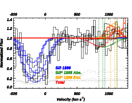
Figure 1: Example of fitting to the absorption and emission lines for Si ii* spectral regions for galaxy J0150+1308 (z = 0.14668). The black and gray histograms are the data and errors, respectively. In each panel, the blueshifted outflow component for the Si ii resonance line is shown in blue (adopted from Xu et al. 2022a; see Section 3.1). The fitted absorption and emission models for Si ii* are shown in green and orange, respectively. The summed model for Si ii* is shown in red. The green and orange dashed lines mark the velocity centers for the fitted absorption and emission lines, respectively. See detailed fitting methods in Section 3.2.

3.2 Measurements of Column Density from Si ii*

Galactic outflows not only show absorption lines from resonance transitions, e.g., Si ii $\lambda$1260, but also from fine structure excited transitions, e.g., Si ii* $\lambda$1265 (e.g., Jaskot et al. 2019). The combination of both can be adopted to derive the electron number density ($n_{\mathrm{\scriptstyle e}}$) of the outflows (see Section 3.3). In this subsection, we focus on measuring N(Si ii*) for galaxies in our sample.

There are a total of six Si ii* lines observable in the rest-frame FUV. We list their important atomic information in Table 1. We find the observed absorption lines from Si ii* are commonly weak in our galaxies. This is consistent with the assumed low $n_{\mathrm{\scriptstyle e}}$ ($\sim$ 10 cm^-3) for typical starburst galaxies (e.g., Xu et al. 2022a). This low $n_{\mathrm{\scriptstyle e}}$ has both pros and cons for our analysis. On the one hand, the weaker Si ii* troughs are generally optically thin ($\tau\ \ll$ 1), and we can safely measure N(Si ii*) by adopting CF = 1, given the apparent optical depth (AOD) assumption (Savage & Sembach 1991). On the other hand, the shallow Si ii* troughs are sometimes difficult to measure, even in our high SNR HST/COS spectra. Another complexity is that the emission lines from Si ii* (i.e., so-called fluorescent lines) can contaminate the blue-shifted absorption troughs of Si ii*, especially when the outflow velocity ($V_{\text{out}}$) is small. The steps for our fitting process of Si ii* lines and measurements of N(Si ii*) are as follows:

1. We fit the fluorescent emission and fine-structure absorption lines from Si ii* $\lambda$1197, 1265, 1309, and 1533 for each galaxy simultaneously. We exclude Si ii* $\lambda$1194 because it is commonly blended with the absorption trough from Si ii $\lambda$1193. For each galaxy, we also exclude Si ii* lines that fall into a chip gap or are contaminated by Galactic lines (e.g., Si ii $\lambda$1197 can be affected by Galactic Ly$\alpha$).

2. For each Si ii* absorption line, we assume it has a Gaussian optical depth profile:

   $$I_{k}(v) =e^{-\tau_{k}(v)}$$ (1)

   $$\tau_{k}(v) =\frac{b_{k}}{\sigma\sqrt{2\pi}}\times exp(\frac{(v-v_{c})^{2}}{2\sigma^{2}})$$

   where $k$ stands for the $k$th Si ii* absorption line, $I_{k}(v)$ is the normalized intensity, $\tau_{k}(v)$ is the optical depth at each velocity of the absorption trough, $\mathit{v}$ is the velocity. Given the AOD assumption, the optical depths of different Si ii* absorption lines (scaled by coefficient $b_{k}$) are linked by their oscillator strength ($f$) ratios (see Table 1). The velocity center (v_c) and dispersion ($\sigma$) of the Si ii* absorption lines are fixed among all Si ii* lines. These fixed values are chosen to be the same as the median values from all Si ii resonance absorption lines (Section 3.1). This assumes that the same outflow clouds have produced Si ii and Si ii* absorption lines, which is true since both lines have close energy levels (Section 3.3).

3. For each Si ii* emission line, we model it using only one Gaussian profile in velocity space. This is because Si ii* in our sample show weak and narrow fluorescent emission-lines, and are inconsistent with arising from the outflowing gas seen in absorption (i.e., broad lines). This implies that most of the emission from the outflow arises on scales larger than the projected COS aperture (Wang et al. 2020). For all Si ii* emission lines, we fix v_c at the systematic velocity, and $\sigma$ is set to be in the range between 0 and the median FWHM of the static ISM component of Si ii resonance lines (Section 3.1). Their amplitudes are free parameters.

4. Then, we conduct $\chi^{2}$ minimization to fit all 2$\times$N profiles simultaneously to the spectral regions of Si ii*. Here the 2 stands for the emission and absorption line for each Si ii*, and N equals the number of Si ii* lines that are clean and used in the fit. We adopt the fitting routine mpfit (Markwardt 2009).

5. Finally, assuming AOD, N(Si ii*) can be derived from the best-fitted $\tau_{k}(v)$ as follows (Savage & Sembach 1991):

   $$N_{ion}(v) =\frac{3.8\times\ 10^{14}}{f_{k}\cdot\lambda_{k}}\cdot\tau_{k}(v)$$ (2)

   $$N_{ion} =\int{N_{ion}(v)}dv$$

   where $\lambda_{k}$ is the wavelength for the $k$th Si ii* line that has $\tau_{k}(v)$. Note that under the AOD assumption, choices of different Si ii* lines in Equation (2) lead to the exact same $N_{\mathrm{\scriptstyle ion}}$.

Table 1: Atomic Data for the Resonance and Excited Transitions of Si ii ^(a)

Ions	Vac. Wave.	flk	Akl	E${}_{\text{low}}$ – E${}_{\text{up}}$
(1)	(2)	(3)	(4)	(5)
Si ii	1190.42	2.77 $\times$ 10-1	6.53 $\times$ 108	0.0 - 10.41
Si ii	1193.29	5.75 $\times$ 10-1	2.69 $\times$ 109	0.0 - 10.39
Si ii	1260.42	1.22	2.57 $\times$ 109	0.0 - 9.84
Si ii	1304.37	9.28 $\times$ 10-2	3.64 $\times$ 108	0.0 - 9.50
Si ii	1526.71	1.33 $\times$ 10-1	3.81 $\times$ 108	0.0 - 8.12
Si ii*	1194.50	7.37 $\times$ 10-1	3.45 $\times$ 109	0.036 - 10.41
Si ii*	1197.39	1.50 $\times$ 10-1	1.40 $\times$ 109	0.036 - 10.39
Si ii*	1264.73(b)	1.09	3.04 $\times$ 109	0.036 - 9.84
Si ii*	1265.02(b)	1.13$\times$ 10-1	4.73 $\times$ 108	0.036 - 9.84
Si ii*	1309.28	8.00 $\times$ 10-2	6.23 $\times$ 108	0.036 - 9.50
Si ii*	1533.45	1.33 $\times$ 10-1	7.52 $\times$ 108	0.036 - 8.12
Note. – (a).  Data are obtained from National Institute of Standards and Technology (NIST) atomic database (Kramida et al. 2018). (2).  Vacuum wavelengths in units of Å. (3).  Oscillator strengths. (4).  Einstein A coefficients in units of s-1. (5).  Energies from lower to upper levels in units of eV. (b).  Si ii* has two close transitions at $\sim$ 1265 Å, i.e., Si ii* $\lambda$1264.73 and $\lambda$1265.02. Both are from the same lower energy level at 0.036 eV, but have slightly different upper energy levels due to fine structure splitting ($\delta E$ $\sim$ 4$\times$10-4 eV). See discussion in Section 3.3.

There are two close transitions of Si ii* at $\sim$ 1265 Å, i.e., Si ii* $\lambda$1264.73 and $\lambda$1265.02. Both are from the same lower energy level at 0.036 eV (= 287.24 cm^-1), but have slightly different upper energy levels due to fine structure splitting ($\delta E$ $\sim$ 4$\times$10^-4 eV). Since the velocity offset between these two lines is only 69 km s^-1, we can barely resolve their absorption lines in the spectra. Thus, we adopt the combined $f$ value in the calculations of N(Si ii*) (Borguet et al. 2012). Since Si ii* $\lambda$1265.02 has $\sim$ 10 times smaller $f$ value than that of Si ii* $\lambda$1264.73 (Table 1), the absorption trough is always dominated by the latter.

An example of the fitted Si ii* spectral regions is shown in Figure 1. The outflow components for the Si ii resonance lines are shown in blue (Section 3.1), while the fitted absorption and emission models for Si ii* are shown in green and orange, respectively. The overall model for Si ii* by summing both the absorption and emission is shown in red. There is a clear absorption trough from Si ii* $\lambda$1265, and it is well-fitted, while there is no trough seen in Si ii* $\lambda$1309. This is as expected since f₁₂₆₅/f₁₃₀₉ = 15, which leads to $\tau_{1265}$/$\tau_{1309}$ = 15 under AOD models. Overall, we have measured N(Si ii*) securely in 11 out of 22 galaxies in our sample. These galaxies that have N(Si ii*) measured yield a mean N(Si ii*)/N(Si ii) $\sim$ 0.01. In Table 3, we report the measured N(Si ii) and N(Si ii*) in column 6 and 7, respectively.

3.3 Mechanisms for Generating Si ii*: Collisions v.s. Radiative Pumping

As shown in Table 1, the observed fine-structure transitions of Si ii* in FUV have lower energy levels as E${}_{\text{low}}$ = 0.036 eV (= 287.24 cm^-1), which is the first excited energy level of Si ii (hereafter, Si ii* specifically stands for this level). Two mechanisms can populate Si ii*: 1) Collisional excitation of the ground state of Si ii  by free electrons (e.g., Silva & Viegas 2002; Osterbrock & Ferland 2006; Borguet et al. 2012). In this case, a higher $n_{\mathrm{\scriptstyle e}}$ would yield a higher n(Si ii*)/n(Si ii) ratio, where n(Si ii*) and n(Si ii) stand for the level population of the first excited and ground state of Si ii. 2) Indirect UV pumping, i.e., the Si ii ground state is excited by absorption of a UV photon to an upper energy level, followed by a spontaneous decay to the excited level at Si ii* 287.24 cm^-1. In this case, a stronger radiation field leads to higher n(Si ii*)/n(Si ii) (see, e.g., Prochaska et al. 2006).

To check if indirect UV pumping can be the dominant mechanism, we estimate the radiation intensity G (in units of ergs cm^-2 s^-1) suffered by outflows for galaxies in our sample. We first measure each galaxy’s continuum flux ($\lambda$F_λ) around Si ii $\lambda$1260. Then we convert it to luminosity as: $\lambda$L_λ = 4$\pi$D${}_{L}^{2}\times\lambda$F_λ, where D_L is the luminosity distance of the galaxy. We conservatively assume the location of observed outflowing gas is at or beyond the starburst radius (i.e., $r_{\text{out}}$ $>$ $r_{*}$), which we will show in Section 4.3 to be a fair assumption. Finally, we derive G for each galaxy as G = $\lambda$L_λ/(4$\pi r_{\text{out}}^{2}$). We find the majority of galaxies in our sample have G/G₀ $<$ 10³ (with two exceptions), while the mean G/G₀ is only $\sim$ 250. Here, G₀ represents the interstellar FUV intensity of our Milky Way (Habing 1968), which is $\sim$ 1.6 $\times$ 10^-3 ergs cm^-2 s^-1.

As shown in Prochaska et al. (2006), n(Si ii*)/n(Si ii) $<$ 10^-4 when G/G₀ $<$ 10³. Given our observed mean N(Si ii*)/N(Si ii) = 0.01, we conclude that indirect UV pumping commonly contribute $<$ 10^-4/0.01 = 1% of the observed population of Si ii*. This is different from the fine structure absorption lines detected in $\gamma$-ray bursts in Prochaska et al. (2006), where indirect UV pumping dominates because the radiation field is much stronger.

Thus, collisional excitation is the dominant mechanism for populating n(Si ii*) in our galaxies. We show the relationship between level population ratio and $n_{\mathrm{\scriptstyle e}}$ in Figure 2 for Si ii. The modelled curves are calculated using the CHIANTI database (v8.0.7, Del Zanna et al. 2015), assuming collisional excitation under three different temperatures. The relation is only weakly dependent on temperature. The critical density ($n_{\mathrm{\scriptstyle cr}}$) for Si ii* is defined at the position where $n$(Si ii*) = $n$(Si ii). For T = 10,000 K, we get $n_{\mathrm{\scriptstyle cr}}$ $\sim$ 2000 cm^-3. From Figure 2, we can derive $n_{\mathrm{\scriptstyle e}}$ from the observed column density ratio of N(Si ii*)/N(Si ii) (e.g., Borguet et al. 2012; Xu et al. 2019). The errors of $n_{\mathrm{\scriptstyle e}}$ are propagated from the errors of N(Si ii*)/N(Si ii).

Given galaxies in our sample have N(Si ii*)/N(Si ii) in the range between $\sim$ 0.001 and $\sim$ 0.1, we get $n_{\mathrm{\scriptstyle e}}$ from a few to $\sim$ 100 cm^-3. The derived $n_{\mathrm{\scriptstyle e}}$ for each galaxy is listed in Table 3. For galaxies that show no absorption on N(Si ii*), we present upper limits on $n_{\mathrm{\scriptstyle e}}$ based on their upper limits of N(Si ii*) (Section 3.2).

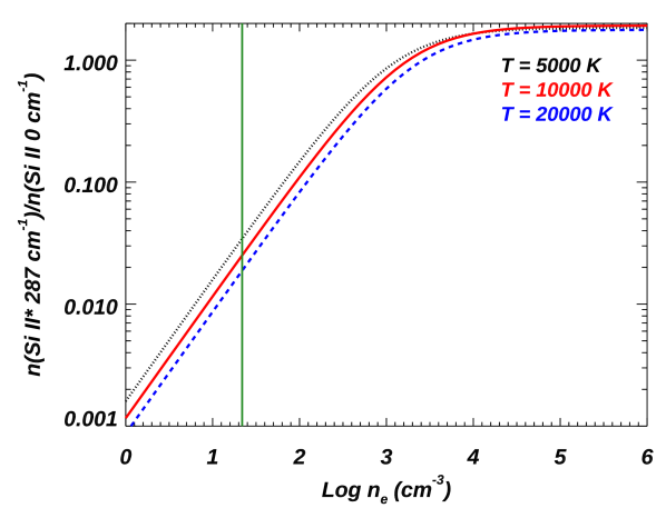
Figure 2: Population ratio of Si ii’s fine structure level (E${}_{\text{low}}$ = 287 cm^-3) to the ground state (E${}_{\text{low}}$ = 0 cm^-3) versus the electron number density ($n_{\mathrm{\scriptstyle e}}$) (e.g., Osterbrock & Ferland 2006). The modelled curves are calculated using the CHIANTI database (v8.0.7, Del Zanna et al. 2015), assuming collisional excitation under three different temperatures. The green vertical line represents the median value of $n_{\mathrm{\scriptstyle e}}$ measured from galaxies in our sample. See Section 3.3 for more discussion.

Table 2: Summary of the Notations and Measured Quantities

Notation	Definition	Reference	Mean	Median	STDDEV(a)
(1)	(2)	(3)	(4)	(5)	(6)
$r_{\text{out}}$	Actual outflow radius distribution	Section 1	…(b)	…	…
$r_{*}$	Starburst radius of the galaxy	Section 1	…	…	…
$r_{n}$	Outflow radius at the derived $n_{\mathrm{\scriptstyle e}}$ from Si ii*	Section 4.2	…(c)	…	…
$n_{\mathrm{\scriptstyle e}}$	Outflow electron number density	Section 4.1	22.3 cm-3	22.8 cm-3	18.7 cm-3
$r_{\text{phot}}$	Outflow radius assuming photoionization	Section 4.3.1	1.6 kpc	1.2 kpc	1.4 kpc
$r_{\text{ram}}$	Outflow radius assuming pressure equilibrium	Section 4.3.2	4.2 kpc	4.1 kpc	2.0 kpc
FF	Outflow volume filling factor	Section 4.4	0.5%	0.4%	0.4%
$R_{\text{cl}}$	Outflow cloud size	Section 4.4	13 pc	5 pc	15 pc
$M_{\text{cl}}$	Outflow cloud mass	Section 4.4	1.1 $\times$ 104 M⊙	202 M⊙	1.0 $\times$ 104 M⊙
Note. – (*).  The first part of this table are the important notations adopted throughout the paper. The second part (beginning with $n_{\mathrm{\scriptstyle e}}$) shows the measured quantities (galaxies with lower and upper limits are excluded). We show the mean, median values, and standard deviations for these quantities. (a).  Standard deviation. (b).  $r_{\text{out}}$ is a range or distribution, which can only be measured from spatially resolved detections of outflows. $r_{\text{out}}$ = $r_{n}$ only when the outflow is a thin bubble (see discussions in Sections 1 and 4.3). (c).  Based on different assumptions, we can measure $r_{n}$ as $r_{\text{phot}}$ or $r_{\text{ram}}$ specifically (illustrated in Section 4.3).

4 Results

We summarize the main notations and measured quantities in this paper at Table 2. We illustrate their details in the following subsections.

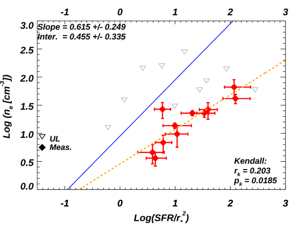
Figure 3: Strong orrelations between outflow electron number density ($n_{\mathrm{\scriptstyle e}}$) and SFR surface density. Galaxies that have $n_{\mathrm{\scriptstyle e}}$ measurement (Mea.) or upper limits (UL) are shown as the red-filled or gray-open symbols, respectively. Kendall’s $\tau$ correlation coefficients are shown at the bottom-right corner of each panel, where we have considered the upper limits following Akritas & Siebert (1996). The best linear-fit to all measurements is shown as the orange dashed line, and the fitted slope and intercept are shown in the top-left corner. The blue line represents the model from Chevalier & Clegg (1985) assuming the outflow gas is in pressure balance with the wind fluid at the radius of the starburst [Equation (12) and Section 4.3.2].

4.1 Outflow Density Distribution and Correlations

In Table 2, we show the statistics of the derived $n_{\mathrm{\scriptstyle e}}$ for 11 galaxies which have secure measurements of their N(Si ii*). We find outflows in the galaxies have the mean and median value $n_{\mathrm{\scriptstyle e}}$ $\sim$ 23 cm^-3. These values are consistent with what has been estimated before from absorption-line data for starburst galaxies (e.g., $n_{\mathrm{\scriptstyle e}}$= 19 – 34 cm^-3 in Chisholm et al. 2018). In Figure 3, we show a strong positive correlation between $n_{\mathrm{\scriptstyle e}}$ with the SFR surface density. We will discuss the implications of this below.

In all Figures in this Section, galaxies in our sample with $n_{\mathrm{\scriptstyle e}}$ measurement or upper limits are shown as red-filled or gray-open symbols, respectively. Kendall’s $\tau$ correlation coefficient ($r_{k}$) and the probability of the null hypothesis ($p_{k}$) are shown at the bottom-right corner. We have taken account of these upper limits in the Kendall $\tau$ test following Akritas & Siebert (1996).

4.2 Interpretations of Outflow Density in Models

Since our HST/COS spectra are integrated over the whole line-of-sight (LOS), the derived $n_{\mathrm{\scriptstyle e}}$ values for outflows also represent mean values over the velocity profile. To better interpret the measured $n_{\mathrm{\scriptstyle e}}$ discussed above, we consider two common outflow models (e.g., Xu et al. 2022a) as follows.

The simplest case for outflow is an expanding thin shell model given a mean electron number density (i.e., $n_{\mathrm{\scriptstyle e}}$ = $n_{\text{s}}$) and shell thickness ($s$). In this case, we have:

$$N(\text{Si II*}) =n(\text{Si II*})\times s$$ (3)

$$N(\text{Si II}) =n(\text{Si II})\times s$$

where $N_{\mathrm{\scriptstyle ion}}$ and $n_{\mathrm{\scriptstyle ion}}$ represent the column and number density for a certain ion, respectively. For galactic outflows, $n_{\mathrm{\scriptstyle e}}$ varies between $\sim$ 10 cm^-3 and $\sim$ 2000 cm^-3 (e.g., Chevalier & Clegg 1985; Yoshida et al. 2019). In this range, the curve in Figure 2 is approximately linear, so we have:

$$\frac{n(\text{Si II*})}{n(\text{Si II})}\approx\frac{n_{\text{e}}}{n_{\text{cr}}}$$ (4)

Combining Equation (3) and (4), we get N(Si ii*)/N(Si ii) $\approx$ $n_{\mathrm{\scriptstyle e}}$/$n_{\mathrm{\scriptstyle cr}}$ = $n_{\text{s}}$/$n_{\mathrm{\scriptstyle cr}}$. Therefore, for a thin shell outflow model, the derived $n_{\mathrm{\scriptstyle e}}$ from N(Si ii*)/N(Si ii) discussed in Section 3.3 is just the mean density in the shell.

In the second case, we consider a mass-conserving galactic wind with constant velocity (e.g., Carr et al. 2021). In this case, the outflow has a density profile $n(r)=n_{0}(r/r_{0})^{-2}$, where $r_{0}$ is the radius at which the outflow begins, and $n_{0}$ is the density at this radius. In this case, we have:

$$N(\text{Si II}) =\int_{r_{0}}^{\infty}n(\text{Si II})dr=\text{C}_{0}\times n_{0}r_{0}$$ (5)

where the integration is from $r_{0}$ to infinity (note n($\infty$) = 0) and C₀ = $n(\text{Si II})_{0}/n_{0}$ is the conversion factor from gas number density to Si ii number density at $r_{0}$. C₀ depends on gas metallicity and ionization. Similarly, for Si ii*, we get:

$$N(\text{Si II*}) =\int_{r_{0}}^{\infty}n(\text{Si II*})dr$$ (6)

$$\approx\int_{r_{0}}^{\infty}\frac{n(r)^{2}}{n_{\text{cr}}}\times\text{C(r)}dr =\frac{C_{0}n^{2}_{0}r_{0}}{3n_{\text{cr}}}$$

where in the second row we have adopted Equation (4) to replace $n$(Si ii*). Thus, this mass-conserving outflow model yields N(Si ii*)/N(Si ii) = $n_{0}$/(3$n_{\mathrm{\scriptstyle cr}}$), i.e., the derived $n_{\mathrm{\scriptstyle e}}$ from Section 3.3 is a third of $n_{0}$. Equivalently, our derived $n_{\mathrm{\scriptstyle e}}$ corresponds to the gas density at $r_{n}=\sqrt{3}r_{0}$. Hereafter, we define $r_{n}$ as the radius of the outflows at which the mean $n_{\mathrm{\scriptstyle e}}$ derived from fine-structure absorption lines above would occur.

Similarly, if we take a general form of $n(r)=n_{0}(r/r_{0})^{-\gamma}$, we get:

$$N(\text{Si II})=\frac{\text{C}_{0}\times n_{0}r_{0}}{(\gamma-1)}$$ (7)

$$N(\text{Si II*})=\frac{C_{0}n^{2}_{0}r_{0}}{(2\gamma-1)n_{\text{cr}}}$$

$$N(\text{Si II*})/N(\text{Si II})=\frac{\gamma-1}{2\gamma-1}\frac{n_{0}}{n_{\text{cr}}}$$

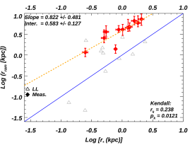
Figure 4: Comparisons of the derived outflow distances with the starburst radius ($r_{*}$). The labels and symbols are the same as Figure 3. Galaxies that have $r$ as a measurement or a lower limit are shown as the red-filled or gray-open symbols, respectively. Left: Derived $r_{phot}$ from photoionization outflow models (Section 4.3.1). Right: Derived $r_{ram}$ by assuming pressure equilibrium (Section 4.3.2). We show the 1:1 correlation as the blue lines. In both cases, the derived $r$ correlate strongly with $r_{*}$.

Thus, in the general form, the derived $n_{\mathrm{\scriptstyle e}}$ from integrated spectra corresponds to $\frac{\gamma-1}{2\gamma-1}n_{0}$. Equivalently, the derived $n_{\mathrm{\scriptstyle e}}$ is the gas density at a radius of $(\frac{2\gamma-1}{\gamma-1})^{\frac{1}{\gamma}}\times$ $r_{0}$. Given the evidence for relatively shallow radial density profiles found in outflows (e.g., Wang et al. 2020; Burchett et al. 2021), we consider the additional cases $\gamma=$ 1.5 and 1.2, and get $r_{n}=2.52~{}r_{0}$ and 5.06 $r_{0}$, respectively. We will compare these sizes with those estimated from our measured values of $n_{\mathrm{\scriptstyle e}}$ below.

We note that if the outflows are more complex than a general form of $n(r)=n_{0}(r/r_{0})^{-\gamma}$, or if there is a range in density at a given radius, the exact interpretation of our measured $n_{\mathrm{\scriptstyle e}}$ and $r_{\text{out}}$ will be different and dependent on the actual form of $n(r)$. We do not dive in this direction, which is beyond the scope of this paper.

4.3 Derivations of Outflow Distances from $n_{\mathrm{\scriptstyle e}}$

For galactic outflows, their radial extent (also referred as the “outflow distance”) can not be determined given only LOS integrated spectra (see, e.g., Wang et al. 2020). In fact, for a continuous outflow, there is no unique way to define distances (e.g., one could define minimum or maximum values, or a half-mass radius, etc.). Moreover, while we have measured a single value for $n_{\mathrm{\scriptstyle e}}$  for a continuous outflow, this value will only apply at some specific radius in the outflow (i.e., $r_{n}$). Here we will estimate $r_{n}$ based on two methods as follows.

4.3.1 Outflow Distances Assuming Photoionization

In star-forming galaxies, the ultraviolet outflow absorption lines (e.g., from O i, Si ii, Si iii, Si iv) have been found to be well-described by photoionization models instead of shock-heating models (Chisholm et al. 2016a). In this case, we have:

$$U_{\mathrm{\scriptstyle H}}=\frac{Q_{\mathrm{\scriptstyle H}}}{4\pi r_{\text{photo}}^{2}n_{\mathrm{\scriptscriptstyle H}}c}\longrightarrow r_{\text{phot}}=\sqrt{\frac{Q_{\mathrm{\scriptstyle H}}}{4\pi U_{\mathrm{\scriptstyle H}}n_{\mathrm{\scriptscriptstyle H}}c}}$$ (8)

where $U_{\mathrm{\scriptstyle H}}$ is the ionization parameter, $Q_{\mathrm{\scriptstyle H}}$ is the source emission rate of ionizing hydrogen photons, $c$ is the speed of light, and $n_{\mathrm{\scriptscriptstyle H}}$ is the hydrogen number density of the outflow. On the right side of the Equation (8), we show the solved formula for outflow distance $r$ assuming photoionization (hereafter, $r_{\text{phot}}$).

For $Q_{\mathrm{\scriptstyle H}}$, we adopt the values from spectral energy distribution (SED) fitting with UV and optical photometry described in Berg et al. (2022). We note that the resulting $Q_{\mathrm{\scriptstyle H}}$ value is the intrinsic value, but only a portion of the ionizing photons can reach the observed outflows due to attenuation by neutral hydrogen and dust. Thus, we estimate the escaped ionizing photon rate ($Q_{\mathrm{\scriptstyle H,esc}}$) as (e.g., Xu et al. 2022b):

$$Q_{\mathrm{\scriptstyle H,esc}}=Q_{\text{H,tot}}\times(1-CF)\times 10^{-0.4E(B-V)k(912)}$$ (9)

where, for each galaxy, $CF$ represents the covering fraction of the static ISM component derived from the absorption line profiles in Xu et al. (2022a), $E(B-V)$ is the internal dust extinction (derived in Berg et al. 2022), and $k(912)$ = 12.87 is the extinction curve at the Lyman limit by assuming the extinction law from Reddy et al. (2016). The second term on the right of Equation (9) represents the attenuation by neutral hydrogen, where a fraction of $CF$ around the galaxy is covered by ISM and is generally optically thick to $Q_{\mathrm{\scriptstyle H}}$. The third term stands for the attenuation by dust. We note that this assumes all the extinction arises inside the starburst and that the outflow is at least as large as the starburst.

For $U_{\mathrm{\scriptstyle H}}$, we adopt the values determined from outflow absorption lines of Si ii and Si iv as described in Xu et al. (2022a). For $n_{\mathrm{\scriptscriptstyle H}}$, we approximate it as $\sim$ $n_{\mathrm{\scriptstyle e}}$/1.2, which is applicable for ionized gas, assuming $\sim$ 90% hydrogen and $\sim$ 9% helium and some metals. Overall, we can solve $r_{\text{phot}}$ from Equation (8). The derived results are shown in Table 3, which are in the range of 0.2 – 5 kpc. In the left panel of Figure 4, we compare the $r_{\text{phot}}$ values with $r_{*}$, which is the commonly assumed outflow radius in the literature (e.g., Heckman et al. 2015; Xu et al. 2022a). We see a strong correlation with $r_{\text{phot}}$$\sim 1$ to 2$r_{*}$ as we move from the smallest to largest galaxies.

4.3.2 Outflow Distances Assuming Pressure Equilibrium

In this section, we compare our data to the simple analytic model for a starburst-driven wind by Chevalier & Clegg (1985) (CC85). To review, CC85 model assumes that massive stars return mass and kinetic energy to the starburst through supernova explosions and stellar winds. These ejecta are thermalized through shocks to form a very hot region of gas inside the starburst. This gas expands through a sonic radius (the starburst radius $r_{*}$) and becomes a high-velocity supersonic wind that can accelerate clouds in its path, producing the blue-shifted absorption lines we see. This latter gas is much denser and cooler than the wind fluid.

The CC85 model requires a density of the wind fluid at its sonic point that depends on SFR/$r_{*}^{2}$. We see this dependence for the absorption-line gas in our data (see Figure 3), so it is worth exploring the connection between the wind fluid and the gas we measure. We begin by comparing the pressures implied by the densities we measure via Si ii to the pressure of the hot wind fluid predicted by CC85 at $r_{*}$. This pressure takes two forms, the thermal pressure of the wind fluid and its ram pressure. In convenient units, at $r_{*}$ the total (summed) pressure is given as:

$$P_{tot}/k=1.79\times 10^{5}\text{SFR}\times r_{*}^{-2}\ [\text{K}\ \text{cm}^{-3}]$$ (10)

where SFR is in units of M_⊙/yr, $r_{*}$ is in units of kpc, and $k$ is the Boltzmann constant. If we assume that the gas we measure with Si ii is in pressure equilibrium with the hot wind fluid, we have:

$$P_{\text{tot}}=2n_{\mathrm{\scriptstyle e}}kT$$ (11)

where $n_{\mathrm{\scriptstyle e}}$ is the density of the outflows, the factor 2 of is due to the gas is highly ionized, and we assume T = 10,000 K, for the gas temperature. Thus, for pressure balance with the wind fluid, the gas densities traced by Si ii at $r_{*}$ are proportional to SFR/$r_{*}^{2}$ as:

$$n_{\mathrm{\scriptstyle e}}\simeq 9\times\text{SFR}\times r_{*}^{-2}[\text{cm}^{-3}]$$ (12)

This allows us to compare the relationship predicted by the model to the data. We show this model as the blue line in the right panel of Figure 3. We see that the densities we measure are about an order-of-magnitude lower than the model. This suggests that we are measuring densities at radii significantly larger than $r_{*}$ where pressures are lower.

In this region, the CC85 model shows that ram pressure is dominant over thermal pressure. Direct measurements of the radial density profiles for the optical emission-line gas show that this material is in pressure balance with the wind ram pressure (Lehnert & Heckman 1996), so this is plausible for the ionized absorption-line gas as well. We can therefore compute the location ($r_{\text{ram}}$) at which the observed absorption-line gas is in pressure balance with the hot wind’s ram pressure:

$$P_{\text{ram}}=\dot{p}_{\text{SFR}}/4\pi r^{2}_{\text{ram}}$$ (13)

where $P_{\text{ram}}$ is the wind ram pressure and $\dot{p}_{\text{SFR}}$ is the total momentum flux of the wind, which equals the input momentum from the starburst [reported in Xu et al. (2022a) for our galaxies].

Combining Equations (11) and (13), we can solve $r_{\text{ram}}$ as:

$$r_{\text{ram}}=\sqrt{\dot{p}_{\text{SFR}}/(8\pi n_{\mathrm{\scriptstyle e}}\ kT)}$$ (14)

The derived results are shown in Table 3, and are in the range $\sim$ 1 to 8 kpc. In the right panel of Figure 4, we compare $r_{\text{ram}}$ with $r_{*}$, which shows a strong correlation. In Figure 5, we also compare $r_{\text{phot}}$ (Section 4.3.1) with $r_{\text{ram}}$ for each object. We find a linear relation with the pressure-based sizes being typically $\sim$ 5 times larger than the starburst radius.

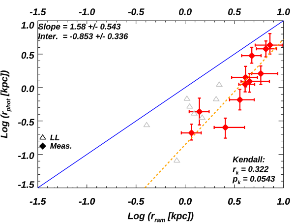
Figure 5: Comparisons between outflow distances ($r$) derived from assuming photoionization (y-axis) and pressure equilibrium (x-axis). The labels and symbols are the same as Figure 3. We find the pressure-based sizes are typically $\sim$ 2 to 5 times larger than the values derived from photoionization models, with the ratio decreasing from the small to large cases.

4.3.3 Outflow Sizes: Summary

We have discussed three estimates of the radius of the outflow at the location at which the measured density occurs,based on different assumptions:

1. The first is based on an outflow with a power-law radial density profile $n(r)=n_{0}(r/r_{0})^{-\gamma}$. It predicts our measured densities occur at the characteristic radius $r_{n}=$ 1.73, 2.52, and 5.06$r_{*}$ for $\gamma$ = 2, 1.5, and 1.2 respectively (Section 4.2). Here $r_{*}$ is the radius of the starburst.

2. The second assumes the gas is photoionized by a fraction of the starburst ionizing flux that reaches the outflow. This estimates that the measured densities occur at a typical distance $\sim 1$ to $2r_{*}$ (Section 4.3.1).

3. Finally, we have assumed that the gas we measure is in pressure balance with the ram pressure of the hot wind fluid. This estimates that the measured densities occur at a typical distance $\sim 4$ to $5r_{*}$ (Section 4.3.2).

Given the systematic uncertainties in these estimates, we regard this level of agreement as satisfactory. In all cases, we are tracing the region of the outflow where densities are high enough to measure with our technique. As explained at the beginning of Section 4.3, the maximum extent of the outflow could be considerably larger than $r_{n}$.

4.4 Other Important Outflow Parameters

Besides the density and structure of outflows, there are various essential parameters of outflows that have rarely been measured from observations. In this sub-section, we constrain these parameters for outflows in our sample. We compare them with simulations of outflows and discuss the implications in Section 5.3.

We start with the volume filling factor (FF) of the observed outflow clouds, where we treat the absorbing material as an ensemble of clouds (e.g., Fielding & Bryan 2022). This yields:

$$\text{FF}=\frac{N_{\text{cl}}\times 4/3\pi R^{3}_{\text{cl}}}{A_{\text{UV}}r_{n}}$$ (15)

where $N_{\text{cl}}$ is the number of outflow clouds entrained in the hot wind at the outflow distance $r_{n}$, and $A_{\text{UV}}$ is the cross-sectional area of the starburst UV continuum. We also have the definition of outflow column density ($N_{\mathrm{\scriptstyle H}}$) as:

$$N_{\mathrm{\scriptstyle H}}\ =\frac{N_{\text{cl}}\times 4/3\pi R^{3}_{\text{cl}}\times n_{\mathrm{\scriptscriptstyle H}}}{A_{\text{UV}}}$$ (16)

One can estimate FF from Equations (15) and (16) as:

$$\text{FF}=\frac{N_{\mathrm{\scriptstyle H}}}{n_{\mathrm{\scriptscriptstyle H}}r_{n}}$$ (17)

where, in this equation, all variables on the right side can be measured for at least part of the galaxies in our sample (see Sections 3.1, 4.1, and 4.3).

In Xu et al. (2022a), we also derived the area covering fraction of the outflow (CF) from the Si ii and Si iv absorption lines (Sections 3.1). We can rewrite CF as:

$$\text{CF}=\beta_{sh}\times\frac{N_{\text{cl}}\times\pi R^{2}_{\text{cl}}}{A_{\text{UV}}}$$ (18)

where $\beta_{sh}$ is a coefficient between 0 and 1 to account for the shadowing effects. This is because the projected areas by different outflow clouds in the LOS can overlap each other so that their total covered area drops by the factor of $\beta_{sh}$. This factor depends on 1) the overall spatial distribution of outflow clouds; and 2) the second term of Equation (18), i.e., the number and relative size of each cloud to A${}_{\text{UV}}$. In Appendix A, we show how to estimate $\beta_{sh}$ from Monte Carlo simulations and the measured CF in Xu et al. (2022a). For the 22 galaxies analyzed in this paper, we get $\beta_{sh}$ in the range of $\sim$ 0.3 to 0.6.

For simplicity of symbols, we define CF_sh = CF/$\beta_{sh}$. From Equations (15) and (18), we can solve the size of the outflow clouds as:

$$R_{\text{cl}}=\frac{3}{4}\frac{\text{FF}}{\text{CF}_{sh}}r_{n}$$ (19)

Using the above expression for FF in Equation (17), this can be rewritten as:

$$R_{\text{cl}}=\frac{3}{4}\frac{N_{\mathrm{\scriptstyle H}}}{n_{\mathrm{\scriptscriptstyle H}}\text{CF}_{sh}}$$ (20)

This shows that $R_{\text{cl}}$ does not depend on $r_{n}$ and can be computed from directly measured quantities. Once we have $R_{\text{cl}}$ constrained, we can combine Equations (18) and (20) to get $N_{\text{cl}}$ as:

$$N_{\text{cl}}=\text{CF}_{sh}\times\frac{A_{\text{UV}}}{\pi R^{2}_{\text{cl}}}=\text{CF}_{sh}\times\frac{R^{2}_{\text{UV}}}{R^{2}_{\text{cl}}}$$ (21)

where $R_{\text{UV}}$ is the UV size of a galaxy and we approximate it as $r_{*}$ that we measured from the HST/COS acquisition images. Note that $N_{\text{cl}}$ is also independent of $r_{n}$. We find the mean and median values of $N_{\text{cl}}$ are 10^5.5 and 10^4.9, respectively.

Finally, we can estimate the average mass of the individual outflow clouds ($M_{\text{cl}}$) by:

$$M_{\text{cl}}=\frac{4}{3}\pi R^{3}_{\text{cl}}n_{\mathrm{\scriptscriptstyle H}}\mu m_{\text{p}}$$ (22)

where $\mu$ $\sim$ 1.4 is the average atomic mass per proton and $m_{\text{p}}$ is the proton mass.

We summarize the statistics for the derived FF, $R_{\text{cl}}$, $M_{\text{cl}}$ values in Table 2, where their values for individual galaxy are shown in the last three columns in Table 3. For FF, which is the only derived parameter dependent on $r_{n}$, we have assumed $r_{n}$ = $r_{\text{ram}}$. If we assume $r_{n}=$ $r_{\text{phot}}$, the derived $R_{\text{cl}}$ and $M_{\text{cl}}$ stay the same, while FF for each galaxy becomes larger with a mean and median value of 1.5% and 13 pc, respectively. In Section 5.3, we compare these measurements with common outflow models, and discuss their implications.

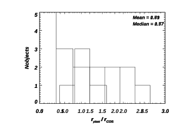
Figure 6: Histograms showing the comparisons between the measured outflow radius ($r_{\text{ram}}$ or $r_{\text{phot}}$) and the projected physical size of the HST/COS aperture for each galaxy. The large ratio of $r_{\text{ram}}$/$r_{\text{COS}}$ suggests that the scattered or fluorescent emission lines should be weak in our galaxies, which is consistent with what has been found in the literature. See details in Section 5.2.

5 Discussion

5.1 Comparisons with Other Outflow Density Measurements

While we are presenting the first examples of density measurements for the warm ionized gas in outflows based on absorption lines, measurements of densities for the optical emission-line gas in outflows have been available in low-redshift starbursts for over thirty years (Heckman et al. 1990). Here we summarize what has been learned from the optical emission-line gas and compare the results to our new data.

For low-redshift starbursts, $n_{\mathrm{\scriptstyle e}}$ is commonly directly measured using the density-sensitive ratio of the [S ii] 6717 and 6731 emission lines. These data can be used to map out the radial variation in $n_{\mathrm{\scriptstyle e}}$, and show a steady radial decline from $\sim 500$ to 1000 cm^-3 in the starburst to $\sim$ 50 to 100 cm^-3 at distances several times larger than $r_{*}$ (e.g., Heckman et al. 1990; Lehnert & Heckman 1996; Yoshida et al. 2019; Perna et al. 2020; Marasco et al. 2022). The [S ii] flux ratio reaches its low-density limit at $n_{e}\sim 10$ to $100$ cm^-3 (Osterbrock & Ferland 2006), so direct measurements of $n_{\mathrm{\scriptstyle e}}$ at larger radii (lower densities) are not possible. This would be consistent with the lower values of $n_{e}$ that we typically get in our sample, if we are probing larger radial scales in this case.

We have shown that with the assumption that the absorbing gas is in pressure balance with the ram pressure of the wind fluid, we do in fact derive large outflow radius. Is this a plausible assumption? We believe it is, because both the emission- and absorption-lines trace the warm ionized gas phase. Since observations establish that the density (and pressure) profiles measured in the emission-line gas are consistent with the radial profile of the wind ram pressure (Heckman et al. 1990; Lehnert & Heckman 1996), this supports adopting the assumption of pressure balance to calculate $R_{\text{ram}}$ (Section 4.3.2).

5.2 Comparisons with Other Measurements of Outflow Structures

The outflow radii we derive assuming ram-pressure confinement are in the range $r_{\text{ram}}\sim$ 1 to 10 kpc. These size scales are consistent with those measured for the outflows traced by optical emission lines for starbursts with a range in SFR similar to our sample (e.g., Armus et al. 1995; Lehnert & Heckman 1996; Martin 1998; Ho et al. 2014; Yoshida et al. 2019). For the sample of dwarf SF galaxies in Marasco et al. (2022), which has weaker SFR than ours ($\sim$ 10 times smaller), they get $r$ $\sim$ 1 kpc. This is around the lower bound of our galaxies as expected from their lower SFR.

Perhaps a more revealing comparison is to the size scales measured using resonantly-scattered emission arising from the same gas that produces the absorption lines seen directly along the LOS to the starburst (Rubin et al. 2011; Martin et al. 2013). This has been done recently using IFU instruments, including VLT/MUSE and Keck/KCWI, to map out Mg ii emission lines surrounding starburst galaxies at intermediate redshifts (e.g., Rupke et al. 2019; Burchett et al. 2021; Zabl et al. 2021; Shaban et al. 2022). These data detect emission out to radii of $\sim$ 10 to 20 kpc, with half-light radii of 5 to 10 kpc. The latter is quite similar to values we derived for $r_{\text{ram}}$ for our sample.

Given a typical aperture size of 1″ – 2″ in current (non-IFU) spectrographs, these sizes imply that a significant fraction of the resonantly scattered line emission could lie outside the aperture. Thus, this missing light helps explain why the scattered (or fluorescently-reprocessed) emission-lines from the outflow are often quite weak (e.g., Erb et al. 2012; Steidel et al. 2018; Wang et al. 2020; Xu et al. 2022a), as can be seen in radiative transfer models of outflows (e.g., Prochaska et al. 2011; Scarlata & Panagia 2015; Carr et al. 2021; and Huberty et al. in prep). We explore this idea further with the current data. In Figure 6, we show histograms of the ratio $r_{\text{ram}}/r_{\text{COS}}$ and $r_{\text{phot}}/r_{\text{COS}}$, where $r_{\text{COS}}$ is the projected physical size of the COS aperture for a given galaxy. We find that the ratios of $r_{\text{ram}}/r_{\text{COS}}$ are $>$ 1, while $r_{\text{phot}}/r_{\text{COS}}$ are most often $\lesssim$ 1. Thus, the larger sizes measured for $r_{\text{ram}}$ may be consistent with the relatively weak emission-lines seen in these galaxies (e.g., Wang et al. 2020; Xu et al. 2022a).

Another apt comparison is to maps of the outflows of neutral gas traced by the Na i D optical absorption-line (1 – 10 kpc, e.g., Martin 2006; Rupke & Veilleux 2013; Perna et al. 2019; Avery et al. 2021; 2022). Our data are complementary to these studies since they pertain to the ionized phase of the outflow and represent integrals over the line-of-sight directly into the starburst. Our data also provide information on key parameters like the densities, filling factors, radii and masses of the outflowing clouds.

Besides the outflows discussed above, SF galaxies can exhibit outflows features in many other wavelength bands and line diagnostics, where outflow distances are measured (see reivews in Heckman & Thompson 2017; Veilleux et al. 2020). These include very hot gas detected in X-ray (at $\sim$ 1 – 10 kpc, e.g., Strickland & Heckman 2007; Li et al. 2011; Zhang et al. 2014), and atomic and molecular outflows observed in infrared to radio bands (e.g., from [C ii] and CO, out to radii of a few kpc, Walter et al. 2002; Chisholm & Matsushita 2016; Stuber et al. 2021).

Again, we emphasize that these various outflow sizes are defined in different ways. In our case, we are defining the size to be the radius at which our measured densities occur. For the emission-line data, the sizes are typically just defined by the radius at which the emission becomes undetectably faint. Additionally, different diagnostics of outflows in different galaxies can reach intrinsically distinct scales, and the relationships between them are not entirely clear. Detailed comparisons are beyond the scope of this paper, but we plan to study the relationships between different diagnostics and phases of galactic outflows in future papers.

5.3 Comparisons with Models and Simulations of Galactic Outflows

Galactic winds are complex and difficult to model because one needs to simultaneously capture the large spatial scales for the whole galaxy and the fundamentally small-scale process happening between the galaxy’s ISM/CGM and the wind (see Naab & Ostriker 2017; and references therein). Currently, a compelling model (e.g., Fielding & Bryan 2022) comprises 1) a hot, volume-filling wind component driven by thermalized ejecta of massive stars (Chevalier & Clegg 1985) and 2) a cold to warm component in the form of embedded clouds, which are entrained by the hot wind. This component produces the observed outflows seen in UV absorption lines (e.g., Xu et al. 2022a). The exchange of mass/momentum/energy between these two components is in the turbulent radiative mixing layer (e.g., Gronke & Oh 2020; Tan et al. 2021; Fielding & Bryan 2022).

Two time-scales control the fate of the outflow clouds (Gronke & Oh 2020): 1) the clouds grow by cooling of the hot wind in a time scale of $t_{\text{cool}}$, which depends mainly on the pressure and metallicity; and 2) the clouds are destroyed by turbulent shredding in a time scale of $t_{\text{mix}}$. We have $t_{\text{mix}}$ $\propto$ $R_{\text{cl}}$/$V_{\text{turb}}$, where $R_{\text{cl}}$ is the average radius of the outflow clouds and $V_{\text{turb}}$ is the turbulent velocity. For large outflow clouds, $t_{\text{cool}}$ $<$ $t_{\text{mix}}$ so that the clouds can grow. For smaller outflow clouds, the clouds are shredded before they can grow. Thus, parameters related to $R_{\text{cl}}$ are important for galactic outflows but have rarely been constrained from observations.

In Section 4.4, we have shown that, based on our measurements of outflow density and distances, we can constrain these parameters, including FF, $R_{\text{cl}}$, and $M_{\text{cl}}$. Here we attempt to compare our measurements to common outflow models.

We can use the criterion derived by Gronke & Oh (2020) for the critical (minimum) size for a cloud to survive/grow when exposed to the ram pressure of the wind:

$$R_{crit}\sim\frac{T_{cl,4}^{5/2}\mathcal{M}_{wind}}{P_{3}\Lambda_{mix,-21.4}}\frac{\chi}{100}\alpha^{-1}pc$$ (23)

Here, $T_{cl,4}$ is the cloud temperature in units of $10^{4}$ K, $\mathcal{M}_{wind}$ is the Mach number of the hot wind fluid, $P_{3}$ is the cloud pressure in units of $10^{3}$ K cm^-3, $\Lambda_{mix,-21.4}$ is the value of the cooling function in the turbulent mixing layer (in units of $10^{-21.4}$ cm³ erg s^-1), $\chi$ is the ratio between the cloud and wind density, and $\alpha$ is a ‘fudge factor’ of order unity. Under this model, if a cloud exposed to the hot wind has smaller sizes than $R_{crit}$, it is destroyed/shredded before being accelerated.

We assume $T_{cl}=10^{4}$ K and can then use our measured values of $n_{\mathrm{\scriptstyle e}}$ to compute $P_{3}$. We further take $\alpha=1$ and the fiducial value of $\Lambda_{mix}$. To measure $\chi$ we adopt the model above for clouds in pressure balance with the wind ram pressure. We use the Chevalier & Clegg (1985) wind solution to obtain $\mathcal{M}_{wind}$ assuming $r_{\text{out}}$ = $r_{\text{ram}}$ (see Section 4.3.2 and left panel of Figure 4). For balancing between the wind ram pressure and the cloud thermal pressure, we have

$$P_{cl}=2n_{cl}kT_{cl}=\rho_{w}v_{w}^{2}$$ (24)

Then, since $\rho_{cl}=n_{cl}m_{p}$, we have:

$$\chi=\frac{\rho_{cl}}{\rho_{w}}=\frac{v_{w}^{2}m_{p}}{2kT_{cl}}$$ (25)

Finally, we adopt the Chevalier & Clegg (1985) model and assume a wind velocity of $v_{w}$ = 1800 km/s (Strickland & Heckman 2009), leading to a value of $\chi\sim 2\times 10^{4}$. We show the results in Figure 7, in which we compare our derived $R_{\text{cl}}$ with $R_{crit}$ for our sample. We find that the estimated values of $R_{\text{cl}}$ all lie close to $R_{crit}$. Within the uncertainties, the growth criterion is satisfied in all 11 cases with $n_{\mathrm{\scriptstyle e}}$ measurements. For the other 11 galaxies with $n_{\mathrm{\scriptstyle e}}$ as upper limits, the derived values of $R_{\text{cl}}$ and $R_{crit}$ are both lower limits (gray-open symbols). However, Equations (20) and (23) show that both sizes are inversely proportional to the density. This means that the ratio of $R_{\text{cl}}$/$R_{crit}$ is independent of density, and thus we can evaluate the growth criterion even in these cases. Within the uncertainties, 20 out of 21 cases satisfy this criterion, i.e., $R_{\text{cl}}$ are large enough for them to survive under the impact of the hot wind.

The fact that the cloud sizes are similar to $R_{crit}$ could be understood if the pre-existing population of clouds initially had a power-law distribution of sizes ($N_{\text{cl}}\propto R_{\text{cl}}^{-\gamma}$) that declines with increasing $R_{\text{cl}}$. Then only the clouds with $R_{\text{cl}}\gtrsim R_{\text{crit}}$ survive the interaction with the wind, while clouds with sizes $\gg$ $R_{crit}$ are rare (i.e., having a small total covering factor).

Additionally, in our assessment of cloud survival, Equations (20) and (23) imply that the ratio of $R_{\text{cl}}$/$R_{crit}$ depends only on the ratio of the column density to covering factor [since we adopted fixed values for all the terms in Equation (23)]. Empirically, there is relatively small variation in CF_sh. In this case, the relatively small spread in the values of $R_{\text{cl}}$/$R_{crit}$ seen in Figure 7 could imply that the total column densities of the absorbing clouds in the outflows are directly connected to the cloud-survival requirement. Future simulations of galactic winds may answer these implications.

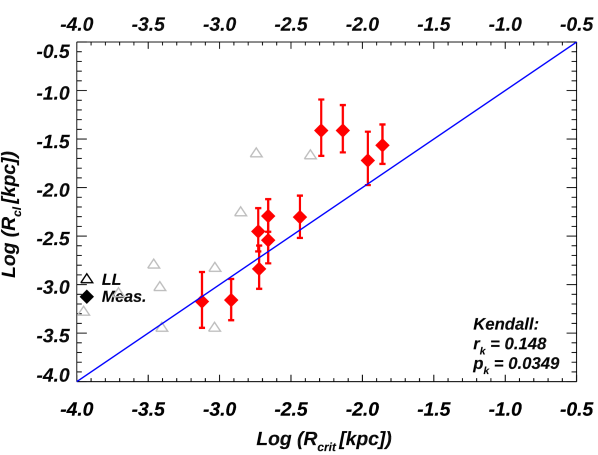
Figure 7: Comparisons of the derived outflowing cloud radii ($R_{\text{cl}}$) with the critical (minimum) radius for a cloud to survive/grow when exposed to the ram pressure of the hot wind (Gronke & Oh 2020). The labels and symbols are the same as Figure 3. Galaxies that have $R_{\text{cl}}$ as measurement or lower limits are shown as the red-filled or gray-open symbols, respectively. The blue line represents the 1:1 relationship. Within the uncertainties, 20/21 outflows have enough cloud sizes large enough to survive. See discussion in Section 5.3.

6 Conclusion and Future Work

We have reported here the first direct measurements of the density ($n_{\mathrm{\scriptstyle e}}$) in outflows from starburst galaxies traced by ultraviolet absorption lines. These measurements were made using COS on HST to measure the ratio of the column density of fine structure excited transitions of Si ii (i.e., Si ii*) to those of the Si ii resonance transitions. The sample of 22 galaxies was drawn from Berg et al. (2022) and Heckman et al. (2015), and limited to cases with SNR $>$ 5, galaxy FUV radii $<$ 1.5″, and detected outflows. Our main results are as follows:

• We were able to measure $n_{\mathrm{\scriptstyle e}}$ in 11 cases and set upper limits in the other 11 galaxies. The median density was 23 cm^-3. We found a strong correlation between $n_{\mathrm{\scriptstyle e}}$ and the star-formation rate per unit area in the starburst.

• Since the value of $n_{\mathrm{\scriptstyle e}}$ is derived along a line-of-sight, its meaning is only simple in the case of an expanding shell with constant density. In the case of a continuous outflow in which the density drops with radius, we showed that for radial density profiles with power-law indices of –2, –1.5, and –1.2, the measured densities would pertain to gas at respective radii of 1.7, 2.5, and 5.1 times the radius at which the outflow begins (taken to be the starburst radius).

• Using the measured values of $n_{\mathrm{\scriptstyle e}}$, we made two indirect estimates of the radius of outflows ($r_{n}$) at which this density applies. The first assumes that the gas is photo-ionized by radiation from the starburst. This required making estimates for the fraction of intrinsic ionizing radiation leaking out of the starburst and into the outflow. Typical radii from this method are 1 to 2 times the starburst radius. We then assumed that the absorbing gas clouds are in pressure equilibrium with the hot wind fluid. These radii are typically 4 to 5 times the starburst radius.

• We used the values of $n_{\mathrm{\scriptstyle e}}$ and our measured values for the total hydrogen column density and the covering fraction of the outflow to estimate the radii and masses of the absorbing clouds. We found median values of $\sim$ 5 pc and 200 M_⊙ respectively. We also estimated the volume filling factor of the population of these clouds, with typical values of $10^{-3}$ to 10^-2.

• We have compared the outflow clouds sizes to theoretical models in which clouds interact with a supersonic wind fluid. We find that in 20 out of 21 cases, the estimated cloud sizes exceed the critical cloud size, meaning that these clouds are predicted to survive and grow as they interact with a hot supersonic wind.

This is the first time that various essential absorption-line outflow parameters have been estimated from observations, including outflow density, volume filling-factor, and cloud sizes/masses. There are plenty of compelling future projects to do in both observations and simulations. For example, how do our derived $n_{\mathrm{\scriptstyle e}}$ and $r_{n}$ values compare to direct measurements from spatially resolved observations? What are the differences and/or connections between the $n_{\mathrm{\scriptstyle e}}$ and outflow sizes measured from emission and absorption line outflows? Given the detected warm outflows, can we provide constraints on the hot wind properties? How can the measured radii and masses of the absorbing clouds help constrain simulations of outflows? We have plans to tackle some of these questions in our future work.

Appendix A Estimations of $\beta_{sh}$

As discussed in Section 4.4, different outflow clouds can “shadow” each other and produce smaller area covering fractions (CF) in the LOS (e.g., Sun et al. 2017; Xu et al. 2020). Here we conduct a Monte Carlo (MC) experiment in two-dimension to estimate the shadowing parameter, $\beta_{sh}$, for Equation (18).

Given $N_{\text{cl}}$ outflow clouds with radius $R_{\text{cl}}$, we randomly distributed them within the area of A${}_{\text{UV}}$. We also assume the ratio of $A_{\text{UV}}/\pi R^{2}_{\text{cl}}=$ 4000. We have tested that the variations of this ratio have little effect on our final results below. We then vary $N_{\text{cl}}$ from 1000 to 15,000 and calculate two quantities: 1) $N_{\text{cl}}\times\pi R^{2}_{\text{cl}}/A_{\text{UV}}$, which represents the CF value if outflow clouds do not shadow each other at all; and 2) the true CF by checking each spot in A${}_{\text{UV}}$ to see if they are covered by any of the outflow clouds. We show these two quantities in the y- and x-axis in Figure 8, respectively.

We find when $N_{\text{cl}}$ grows, the true CF initially increases fast but then slows down. This is because when $N_{\text{cl}}$ is small, we do not expect to have strong shadowing effects given the relatively large area of A${}_{\text{UV}}$ compared to the projected size of each outflow cloud (i.e., $\pi R^{2}_{\text{cl}}$). But when $N_{\text{cl}}$ is large ($\gtrsim$ 4000), the shadowing effects become more significant and the growth of the true CF is slower.

For galaxies in our sample, we have measured the true CF from “down-the-barrel” observations of UV absorption lines (Xu et al. 2022a). Thus, we can estimate y = $N_{\text{cl}}\times\pi R^{2}_{\text{cl}}/A_{\text{UV}}$ for each galaxy based on the true CF and the curve in Figure 8. Then we can calculate $\beta_{sh}$ from Equation (18). For the 22 galaxies analyzed in this paper, we get $\beta_{sh}$ in the range of $\sim$ 0.3 to 0.6.

Figure 8: Comparisons between CF assuming no shadowing versus the true CF from MC simulations. We also show the number of clouds ($N_{\text{cl}}$) for several positions on the line. See discussion in Appendix A.

Appendix B Tables

Here we present the tables for the derived quantities for each galaxy.

Table 3: Measured Parameters for Galaxies in the Combined Sample⁽¹⁾

Object	log(SFR)	log($r_{*}$)	log($N_{\mathrm{\scriptstyle H}}$)	CF(Si ii)	N(Si ii)	N(Si ii*)	log($n_{\mathrm{\scriptstyle e}}$)	A${}_{\text{dust}}$	log(Q${}_{\text{eff}}$)	log($r_{\text{phot}}$)	log($r_{\text{ram}}$)	log(FF)	log(R${}_{\text{Cloud}}$)	log(M${}_{\text{Cloud}}$)	$\beta_{sh}$
	M⊙/yr	kpc	cm-2		1012cm-2	1012cm-2	cm-3	mags.	s-1	kpc	kpc		kpc	M⊙
(1)	(2)	(3)	(4)	(5)	(6)	(7)	(8)	(9)	(10)	(11)	(12)	(13)	(14)	(15)	(16)
J0021+0052	1.07	-0.05	20.78	0.30	243.40	¡62.55	¡2.41	1.81	52.76	¿-1.09	¿-0.09	¿-2.93	¿-3.09	¿1.20	0.56
J0150+1308${}^{\text{(H15)}}$	1.50	0.10	20.67	0.85	720.63	18.89${}^{+0.50}_{-0.50}$	1.36${}^{+0.04}_{-0.05}$	2.81	53.80	0.09${}^{+0.12}_{-0.16}$	0.65${}^{+0.20}_{-0.09}$	-2.73${}^{+0.10}_{-0.21}$	-2.54${}^{+0.24}_{-0.24}$	1.81${}^{+0.73}_{-0.72}$	0.38
J0808+3948	1.26	-0.59	19.99	0.40	741.47	¡45.28	¡1.73	2.07	54.10	¿0.04	¿0.35	¿-3.49	¿-3.45	¿-0.54	0.46
J0823+2806	1.48	-0.30	20.56	0.96	187.19	13.89${}^{+4.50}_{-4.50}$	1.82${}^{+0.13}_{-0.18}$	3.46	53.09	-0.60${}^{+0.14}_{-0.16}$	0.41${}^{+0.19}_{-0.11}$	-3.06${}^{+0.22}_{-0.24}$	-3.18${}^{+0.30}_{-0.27}$	0.35${}^{+0.92}_{-0.83}$	0.34
J0926+4427	1.03	0.12	20.90	0.30	999.09	7.93${}^{+0.71}_{-0.71}$	0.84${}^{+0.13}_{-0.18}$	1.21	53.98	0.48${}^{+0.13}_{-0.11}$	0.68${}^{+0.09}_{-0.10}$	-2.01${}^{+0.22}_{-0.18}$	-1.41${}^{+0.26}_{-0.23}$	4.67${}^{+0.80}_{-0.70}$	0.56
J0938+5428	1.05	0.01	20.86	0.34	1282.70	14.40${}^{+1.93}_{-1.93}$	0.99${}^{+0.15}_{-0.23}$	1.00	53.59	0.15${}^{+0.16}_{-0.14}$	0.61${}^{+0.12}_{-0.14}$	-2.14${}^{+0.28}_{-0.20}$	-1.41${}^{+0.32}_{-0.26}$	4.81${}^{+0.97}_{-0.82}$	0.61
J1016+3754	-1.17	-0.61	20.74	0.25	44.12	¡18.21	¡2.65	0.68	51.99	¿-1.54	¿-1.33	¿-1.97	¿-3.29	¿0.85	0.59
J1024+0524	0.21	-0.27	21.00	0.62	384.52	¡59.64	¡2.16	0.90	53.09	¿-0.56	¿-0.39	¿-2.16	¿-2.80	¿1.81	0.48
J1025+3622	1.04	0.20	20.84	0.69	612.97	2.57${}^{+0.67}_{-0.67}$	0.56${}^{+0.11}_{-0.14}$	1.65	53.83	0.58${}^{+0.12}_{-0.12}$	0.82${}^{+0.11}_{-0.10}$	-1.93${}^{+0.17}_{-0.16}$	-1.56${}^{+0.21}_{-0.19}$	3.95${}^{+0.65}_{-0.59}$	0.38
J1144+4012	1.51	0.26	20.71	0.92	1482.90	23.40${}^{+1.06}_{-1.06}$	1.14${}^{+0.04}_{-0.05}$	2.92	53.68	0.21${}^{+0.11}_{-0.16}$	0.77${}^{+0.17}_{-0.09}$	-2.59${}^{+0.11}_{-0.18}$	-2.30${}^{+0.22}_{-0.21}$	2.31${}^{+0.67}_{-0.65}$	0.37
J1148+2546	0.53	0.37	21.06	0.87	1615.60	¡21.59	¡1.06	2.98	52.76	¿-0.18	¿0.31	¿-1.71	¿-1.67	¿4.10	0.47
J1150+1501	-1.33	-0.87	20.71	0.71	380.18	¡53.65	¡2.12	2.07	51.23	¿-1.54	¿-1.14	¿-1.65	¿-3.04	¿1.07	0.49
J1200+1343	0.75	-0.35	20.85	0.84	789.16	¡47.91	¡1.73	2.58	53.17	¿-0.39	¿0.09	¿-2.37	¿-2.83	¿1.30	0.33
J1253–0312	0.56	-0.11	21.00	0.91	404.83	12.42${}^{+2.38}_{-2.38}$	1.43${}^{+0.12}_{-0.16}$	2.51	52.96	-0.36${}^{+0.20}_{-0.20}$	0.14${}^{+0.10}_{-0.10}$	-1.96${}^{+0.20}_{-0.16}$	-2.44${}^{+0.24}_{-0.21}$	2.17${}^{+0.73}_{-0.64}$	0.29
J1359+5726	0.42	0.17	21.05	0.81	979.65	¡39.70	¡1.55	1.35	53.31	¿-0.17	¿0.02	¿-1.91	¿-2.26	¿2.85	0.43
J1416+1223	1.57	-0.26	20.27	0.54	175.12	8.24${}^{+0.71}_{-0.71}$	1.62${}^{+0.07}_{-0.09}$	2.20	53.63	-0.18${}^{+0.16}_{-0.15}$	0.56${}^{+0.15}_{-0.11}$	-3.29${}^{+0.14}_{-0.17}$	-3.15${}^{+0.22}_{-0.21}$	0.22${}^{+0.66}_{-0.63}$	0.40
J1428+1653	1.22	0.32	20.70	0.62	436.32	2.32${}^{+0.77}_{-0.77}$	0.66${}^{+0.14}_{-0.20}$	1.04	54.26	0.63${}^{+0.17}_{-0.13}$	0.86${}^{+0.13}_{-0.15}$	-2.21${}^{+0.26}_{-0.19}$	-1.72${}^{+0.30}_{-0.25}$	3.58${}^{+0.90}_{-0.79}$	0.43
J1429+0643	1.42	-0.06	20.81	0.67	675.03	17.69${}^{+0.78}_{-0.78}$	1.36${}^{+0.06}_{-0.07}$	1.58	53.80	0.05${}^{+0.09}_{-0.11}$	0.61${}^{+0.10}_{-0.06}$	-2.55${}^{+0.11}_{-0.13}$	-2.29${}^{+0.17}_{-0.16}$	2.55${}^{+0.53}_{-0.49}$	0.44
J1448–0110	0.39	-0.60	20.50	0.83	106.60	3.22${}^{+0.92}_{-0.92}$	1.42${}^{+0.12}_{-0.17}$	2.76	52.45	-0.68${}^{+0.13}_{-0.11}$	0.06${}^{+0.10}_{-0.10}$	-2.38${}^{+0.20}_{-0.16}$	-2.84${}^{+0.24}_{-0.20}$	0.96${}^{+0.73}_{-0.64}$	0.34
J1545+0858	0.37	-0.31	21.38	0.61	1435.50	¡45.45	¡1.44	1.55	53.12	¿-0.29	¿0.05	¿-1.50	¿-1.66	¿4.53	0.51
J1612+0817	1.58	0.01	…	0.80	2665.30	¡230.03	¡1.89	2.75	53.83	…	¿0.42	…	…	…	…
J2103–0728${}^{\text{(H15)}}$	1.29	-0.32	20.47	0.84	1526.10	¡209.23	¡2.10	4.18	53.43	¿-0.45	¿0.17	¿-3.20	¿-3.44	¿-0.16	0.40
Notes: (1)  Measured parameters for 22 galaxies in our combined sample that have high SNR spectra of Si ii and Si ii* (see Section 3.2). Galaxies from Heckman et al. (2015) is marked as (H15). Descriptions for each column: (2) – (6) are adopted from Xu et al. (2022a) (see Section 3.1 for a summary); (2) The log of star-formation rate (SFR) of the galaxy; (3) The log of starburst radius of the galaxy, where we take $r_{*}$ = 2 $\times r_{\text{50}}$ from Xu et al. (2022a); (4) The log of total hydrogen column density of the outflow; (5) The mean covering fraction derived from Si ii outflow absorption lines; (6) The column density of Si ii in the outflows; (7) The column density of excited states of Si ii (i.e., Si ii*) measured in the outflow absorption troughs for each galaxy (Section 3.2); (8) The log of electron number density of the outflows (Section 3.3); (9) Dust extinction derived from SED fittings (Section 4.3.1); (10): The effective ionizing photon rate per second for the outflows (Section 4.3.1); (11) The radius of the observed outflows derived from photoionization models (Section 4.3.1); (12) The radius of the observed outflows derived from assuming pressure equilibrium (Section 4.3.2); (13) The volume filling factor for outflows (Section 4.4); (14) and (15) The average radius and mass of the outflowing clouds (Section 4.4) adopting $r_{\text{ram}}$ (Section 4.4). (16) The coeffcient between 0 –1 to account for the shadowing effects of outflow clouds (see Section 4.4 and Appendix A)

References

- Akritas & Siebert (1996) Akritas, M. G., & Siebert, J. 1996, MNRAS, 278, 919, doi: 10.1093/mnras/278.4.919
- Armus et al. (1995) Armus, L., Heckman, T. M., Weaver, K. A., & Lehnert, M. D. 1995, ApJ, 445, 666, doi: 10.1086/175729
- Astropy Collaboration et al. (2022) Astropy Collaboration, Price-Whelan, A. M., Lim, P. L., et al. 2022, ApJ, 935, 167, doi: 10.3847/1538-4357/ac7c74
- Avery et al. (2021) Avery, C. R., Wuyts, S., Förster Schreiber, N. M., et al. 2021, MNRAS, 503, 5134, doi: 10.1093/mnras/stab780
- Avery et al. (2022) —. 2022, MNRAS, 511, 4223, doi: 10.1093/mnras/stac190
- Bennett et al. (2014) Bennett, C. L., Larson, D., Weiland, J. L., & Hinshaw, G. 2014, ApJ, 794, 135, doi: 10.1088/0004-637X/794/2/135
- Berg et al. (2022) Berg, D. A., James, B. L., King, T., et al. 2022, arXiv e-prints, arXiv:2203.07357. https://arxiv.org/abs/2203.07357
- Borguet et al. (2012) Borguet, B. C. J., Edmonds, D., Arav, N., Dunn, J., & Kriss, G. A. 2012, The Astrophysical Journal, 751, 107, doi: 10.1088/0004-637x/751/2/107
- Burchett et al. (2021) Burchett, J. N., Rubin, K. H. R., Prochaska, J. X., et al. 2021, ApJ, 909, 151, doi: 10.3847/1538-4357/abd4e0
- Carr et al. (2021) Carr, C., Scarlata, C., Henry, A., & Panagia, N. 2021, ApJ, 906, 104, doi: 10.3847/1538-4357/abc7c3
- Carr et al. (2018) Carr, C., Scarlata, C., Panagia, N., & Henry, A. 2018, ApJ, 860, 143, doi: 10.3847/1538-4357/aac48e
- Cazzoli et al. (2014) Cazzoli, S., Arribas, S., Colina, L., et al. 2014, A&A, 569, A14, doi: 10.1051/0004-6361/201323296
- Chevalier & Clegg (1985) Chevalier, R. A., & Clegg, A. W. 1985, Nature, 317, 44, doi: 10.1038/317044a0
- Chisholm & Matsushita (2016) Chisholm, J., & Matsushita, S. 2016, ApJ, 830, 72, doi: 10.3847/0004-637X/830/2/72
- Chisholm et al. (2019) Chisholm, J., Rigby, J. R., Bayliss, M., et al. 2019, ApJ, 882, 182, doi: 10.3847/1538-4357/ab3104
- Chisholm et al. (2018) Chisholm, J., Tremonti, C., & Leitherer, C. 2018, MNRAS, 481, 1690, doi: 10.1093/mnras/sty2380
- Chisholm et al. (2017) Chisholm, J., Tremonti, C. A., Leitherer, C., & Chen, Y. 2017, MNRAS, 469, 4831, doi: 10.1093/mnras/stx1164
- Chisholm et al. (2016a) Chisholm, J., Tremonti, C. A., Leitherer, C., Chen, Y., & Wofford, A. 2016a, MNRAS, 457, 3133, doi: 10.1093/mnras/stw178
- Chisholm et al. (2015) Chisholm, J., Tremonti, C. A., Leitherer, C., et al. 2015, ApJ, 811, 149, doi: 10.1088/0004-637X/811/2/149
- Chisholm et al. (2016b) Chisholm, J., Tremonti Christy, A., Leitherer, C., & Chen, Y. 2016b, MNRAS, 463, 541, doi: 10.1093/mnras/stw1951
- Dalcanton (2007) Dalcanton, J. J. 2007, ApJ, 658, 941, doi: 10.1086/508913
- Del Zanna et al. (2015) Del Zanna, G., Dere, K. P., Young, P. R., Landi, E., & Mason, H. E. 2015, A&A, 582, A56, doi: 10.1051/0004-6361/201526827
- Erb et al. (2012) Erb, D. K., Quider, A. M., Henry, A. L., & Martin, C. L. 2012, ApJ, 759, 26, doi: 10.1088/0004-637X/759/1/26
- Ferland et al. (2017) Ferland, G. J., Chatzikos, M., Guzmán, F., et al. 2017, Rev. Mexicana Astron. Astrofis., 53, 385. https://arxiv.org/abs/1705.10877
- Fielding & Bryan (2022) Fielding, D. B., & Bryan, G. L. 2022, ApJ, 924, 82, doi: 10.3847/1538-4357/ac2f41
- Fluetsch et al. (2021) Fluetsch, A., Maiolino, R., Carniani, S., et al. 2021, MNRAS, 505, 5753, doi: 10.1093/mnras/stab1666
- Gronke & Oh (2020) Gronke, M., & Oh, S. P. 2020, MNRAS, 492, 1970, doi: 10.1093/mnras/stz3332
- Habing (1968) Habing, H. J. 1968, Bull. Astron. Inst. Netherlands, 19, 421
- Heckman et al. (2017) Heckman, T., Borthakur, S., Wild, V., Schiminovich, D., & Bordoloi, R. 2017, ApJ, 846, 151, doi: 10.3847/1538-4357/aa80dc
- Heckman et al. (2015) Heckman, T. M., Alexandroff, R. M., Borthakur, S., Overzier, R., & Leitherer, C. 2015, ApJ, 809, 147, doi: 10.1088/0004-637X/809/2/147
- Heckman et al. (1990) Heckman, T. M., Armus, L., & Miley, G. K. 1990, ApJS, 74, 833, doi: 10.1086/191522
- Heckman & Borthakur (2016) Heckman, T. M., & Borthakur, S. 2016, ApJ, 822, 9, doi: 10.3847/0004-637X/822/1/9
- Heckman et al. (2000) Heckman, T. M., Lehnert, M. D., Strickland, D. K., & Armus, L. 2000, ApJS, 129, 493, doi: 10.1086/313421
- Heckman & Thompson (2017) Heckman, T. M., & Thompson, T. A. 2017, arXiv e-prints, arXiv:1701.09062. https://arxiv.org/abs/1701.09062
- Heckman et al. (2011) Heckman, T. M., Borthakur, S., Overzier, R., et al. 2011, ApJ, 730, 5, doi: 10.1088/0004-637X/730/1/5
- Ho et al. (2014) Ho, I. T., Kewley, L. J., Dopita, M. A., et al. 2014, MNRAS, 444, 3894, doi: 10.1093/mnras/stu1653
- Hogarth et al. (2020) Hogarth, L., Amor ́in, R., V ́ilchez, J. M., et al. 2020, MNRAS, 494, 3541, doi: 10.1093/mnras/staa851
- Hopkins et al. (2012) Hopkins, P. F., Quataert, E., & Murray, N. 2012, MNRAS, 421, 3522, doi: 10.1111/j.1365-2966.2012.20593.x
- James et al. (2022) James, B. L., Berg, D. A., King, T., et al. 2022, ApJ
- Jaskot et al. (2019) Jaskot, A. E., Dowd, T., Oey, M. S., Scarlata, C., & McKinney, J. 2019, ApJ, 885, 96, doi: 10.3847/1538-4357/ab3d3b
- Kluyver et al. (2016) Kluyver, T., Ragan-Kelley, B., Pérez, F., et al. 2016, in IOS Press, 87–90, doi: 10.3233/978-1-61499-649-1-87
- Kramida et al. (2018) Kramida, A., Ralchenko, Y., Nave, G., & Reader, J. 2018, in APS Meeting Abstracts, Vol. 2018, APS Division of Atomic, Molecular and Optical Physics Meeting Abstracts, M01.004
- Lehnert & Heckman (1996) Lehnert, M. D., & Heckman, T. M. 1996, ApJ, 462, 651, doi: 10.1086/177180
- Leitherer et al. (2010) Leitherer, C., Ortiz Otálvaro, P. A., Bresolin, F., et al. 2010, ApJS, 189, 309, doi: 10.1088/0067-0049/189/2/309
- Leitherer et al. (1999) Leitherer, C., Schaerer, D., Goldader, J. D., et al. 1999, ApJS, 123, 3, doi: 10.1086/313233
- Li et al. (2011) Li, Z., Jones, C., Forman, W. R., et al. 2011, ApJ, 730, 84, doi: 10.1088/0004-637X/730/2/84
- Marasco et al. (2022) Marasco, A., Belfiore, F., Cresci, G., et al. 2022, arXiv e-prints, arXiv:2209.02726. https://arxiv.org/abs/2209.02726
- Markwardt (2009) Markwardt, C. B. 2009, in Astronomical Society of the Pacific Conference Series, Vol. 411, Astronomical Data Analysis Software and Systems XVIII, ed. D. A. Bohlender, D. Durand, & P. Dowler, 251. https://arxiv.org/abs/0902.2850
- Martin (1998) Martin, C. L. 1998, ApJ, 506, 222, doi: 10.1086/306219
- Martin (2005) —. 2005, ApJ, 621, 227, doi: 10.1086/427277
- Martin (2006) —. 2006, ApJ, 647, 222, doi: 10.1086/504886
- Martin et al. (2012) Martin, C. L., Shapley, A. E., Coil, A. L., et al. 2012, ApJ, 760, 127, doi: 10.1088/0004-637X/760/2/127
- Martin et al. (2013) —. 2013, ApJ, 770, 41, doi: 10.1088/0004-637X/770/1/41
- Mingozzi et al. (2022) Mingozzi, M., James, B. L., Arellano-Córdova, K. Z., et al. 2022, arXiv e-prints, arXiv:2209.09047. https://arxiv.org/abs/2209.09047
- Naab & Ostriker (2017) Naab, T., & Ostriker, J. P. 2017, ARA&A, 55, 59, doi: 10.1146/annurev-astro-081913-040019
- Nguyen et al. (2023) Nguyen, D. D., Thompson, T. A., Schneider, E. E., Lopez, S., & Lopez, L. A. 2023, MNRAS, 518, L87, doi: 10.1093/mnrasl/slac141
- Osterbrock & Ferland (2006) Osterbrock, D. E., & Ferland, G. J. 2006, Astrophysics of gaseous nebulae and active galactic nuclei
- Perna et al. (2019) Perna, M., Cresci, G., Brusa, M., et al. 2019, A&A, 623, A171, doi: 10.1051/0004-6361/201834193
- Perna et al. (2020) Perna, M., Arribas, S., Catalán-Torrecilla, C., et al. 2020, A&A, 643, A139, doi: 10.1051/0004-6361/202038328
- Prochaska et al. (2006) Prochaska, J. X., Chen, H.-W., & Bloom, J. S. 2006, ApJ, 648, 95, doi: 10.1086/505737
- Prochaska et al. (2011) Prochaska, J. X., Kasen, D., & Rubin, K. 2011, ApJ, 734, 24, doi: 10.1088/0004-637X/734/1/24
- Reddy et al. (2016) Reddy, N. A., Steidel, C. C., Pettini, M., Bogosavljević, M., & Shapley, A. E. 2016, ApJ, 828, 108, doi: 10.3847/0004-637X/828/2/108
- Rubin et al. (2014) Rubin, K. H. R., Prochaska, J. X., Koo, D. C., et al. 2014, ApJ, 794, 156, doi: 10.1088/0004-637X/794/2/156
- Rubin et al. (2011) Rubin, K. H. R., Prochaska, J. X., Ménard, B., et al. 2011, ApJ, 728, 55, doi: 10.1088/0004-637X/728/1/55
- Rupke (2018) Rupke, D. 2018, Galaxies, 6, 138, doi: 10.3390/galaxies6040138
- Rupke et al. (2005) Rupke, D. S., Veilleux, S., & Sanders, D. B. 2005, ApJS, 160, 87, doi: 10.1086/432886
- Rupke & Veilleux (2013) Rupke, D. S. N., & Veilleux, S. 2013, ApJ, 768, 75, doi: 10.1088/0004-637X/768/1/75
- Rupke et al. (2019) Rupke, D. S. N., Coil, A., Geach, J. E., et al. 2019, Nature, 574, 643, doi: 10.1038/s41586-019-1686-1
- Saldana-Lopez et al. (2022) Saldana-Lopez, A., Schaerer, D., Chisholm, J., et al. 2022, arXiv e-prints, arXiv:2201.11800. https://arxiv.org/abs/2201.11800
- Savage & Sembach (1991) Savage, B. D., & Sembach, K. R. 1991, ApJ, 379, 245, doi: 10.1086/170498
- Scarlata & Panagia (2015) Scarlata, C., & Panagia, N. 2015, ApJ, 801, 43, doi: 10.1088/0004-637X/801/1/43
- Shaban et al. (2022) Shaban, A., Bordoloi, R., Chisholm, J., et al. 2022, ApJ, 936, 77, doi: 10.3847/1538-4357/ac7c65
- Silva & Viegas (2002) Silva, A. I., & Viegas, S. M. 2002, MNRAS, 329, 135, doi: 10.1046/j.1365-8711.2002.04956.x
- Steidel et al. (2018) Steidel, C. C., Bogosavljević, M., Shapley, A. E., et al. 2018, ApJ, 869, 123, doi: 10.3847/1538-4357/aaed28
- Steidel et al. (2010) Steidel, C. C., Erb, D. K., Shapley, A. E., et al. 2010, ApJ, 717, 289, doi: 10.1088/0004-637X/717/1/289
- Strickland & Heckman (2007) Strickland, D. K., & Heckman, T. M. 2007, ApJ, 658, 258, doi: 10.1086/511174
- Strickland & Heckman (2009) —. 2009, ApJ, 697, 2030, doi: 10.1088/0004-637X/697/2/2030
- Stuber et al. (2021) Stuber, S. K., Saito, T., Schinnerer, E., et al. 2021, A&A, 653, A172, doi: 10.1051/0004-6361/202141093
- Sun et al. (2017) Sun, L., Zhou, H., Ji, T., et al. 2017, ApJ, 838, 88, doi: 10.3847/1538-4357/aa63eb
- Tan et al. (2021) Tan, B., Oh, S. P., & Gronke, M. 2021, MNRAS, 502, 3179, doi: 10.1093/mnras/stab053
- Veilleux et al. (2005) Veilleux, S., Cecil, G., & Bland-Hawthorn, J. 2005, ARA&A, 43, 769, doi: 10.1146/annurev.astro.43.072103.150610
- Veilleux et al. (2020) Veilleux, S., Maiolino, R., Bolatto, A. D., & Aalto, S. 2020, A&A Rev., 28, 2, doi: 10.1007/s00159-019-0121-9
- Walter et al. (2002) Walter, F., Weiss, A., & Scoville, N. 2002, ApJ, 580, L21, doi: 10.1086/345287
- Wang et al. (2020) Wang, B., Heckman, T. M., Zhu, G., & Norman, C. A. 2020, ApJ, 894, 149, doi: 10.3847/1538-4357/ab88b4
- Wood et al. (2015) Wood, C. M., Tremonti, C. A., Calzetti, D., et al. 2015, MNRAS, 452, 2712, doi: 10.1093/mnras/stv1471
- Wright (2006) Wright, E. L. 2006, PASP, 118, 1711, doi: 10.1086/510102
- Xu et al. (2019) Xu, X., Arav, N., Miller, T., & Benn, C. 2019, ApJ, 876, 105, doi: 10.3847/1538-4357/ab164e
- Xu et al. (2020) Xu, X., Arav, N., Miller, T., Kriss, G. A., & Plesha, R. 2020, ApJS, 247, 38, doi: 10.3847/1538-4365/ab596a
- Xu et al. (2022a) Xu, X., Heckman, T., Henry, A., et al. 2022a, ApJ, 933, 222, doi: 10.3847/1538-4357/ac6d56
- Xu et al. (2022b) Xu, X., Henry, A., Heckman, T., et al. 2022b, ApJ, 933, 202, doi: 10.3847/1538-4357/ac7225
- Yoshida et al. (2019) Yoshida, M., Kawabata, K. S., Ohyama, Y., Itoh, R., & Hattori, T. 2019, PASJ, 71, 87, doi: 10.1093/pasj/psz069
- Zabl et al. (2021) Zabl, J., Bouché, N. F., Wisotzki, L., et al. 2021, MNRAS, 507, 4294, doi: 10.1093/mnras/stab2165
- Zhang et al. (2014) Zhang, D., Thompson, T. A., Murray, N., & Quataert, E. 2014, ApJ, 784, 93, doi: 10.1088/0004-637X/784/2/93