Change point detection and inference in multivariable nonparametric models under mixing conditions

Abstract

This paper studies multivariate nonparametric change point localization and inference problems. The data consists of a multivariate time series with potentially short range dependence. The distribution of this data is assumed to be piecewise constant with densities in a Hölder class. The change points, or times at which the distribution changes, are unknown. We derive the limiting distributions of the change point estimators when the minimal jump size vanishes or remains constant, a first in the literature on change point settings. We are introducing two new features: a consistent estimator that can detect when a change is happening in data with short-term dependence, and a consistent block-type long-run variance estimator. Numerical evidence is provided to back up our theoretical results.

1 Introduction

In this paper, we study the problem of change point detection in nonparametric settings. Our model assumes that a vector of measurements is collected at every time point following a distribution that has a probability density function belonging to a Hölder function class. The change point assumption implies that the probability density functions remain the same across time except for abrupt changes at the change points. Furthermore, our theory permits temporal dependence of the measurements, a feature not explored in prior work.

To be more specific, the observations $\{X_{t}\}_{t=1}^{T}\subset\mathbb{R}^{p}$ are assumed to be an $\alpha$-mixing sequence of random vectors with unknown distributions $\{P_{t}\}_{t=1}^{T}$. The $\alpha$-mixing coefficients, $\{\alpha_{k}\}_{k\in\mathbb{Z}}$, have an exponential-decay,

$$\alpha_{k}\leq e^{-2ck},\quad k\in\mathbb{Z},$$ (1)

for a certain $c>0.$ The decay rate of $\alpha_{k}$ imposes a temporal dependence between events that are separated by $k$ time points, as is stated in (1). This is a standard requirement in the literature (e.g Abadi, 2004; Merlevède et al., 2009). To model the nonstationarity of sequentially observed multivariate data, we assume that there exists $K\in\mathbb{N}$ change points, namely $\{\eta_{k}\}_{k=1}^{K}\subset\{2,...,T\}$ with $1=\eta_{0}<\eta_{1}<\ldots<\eta_{k}\leq T<\eta_{K+1}=T+1$, such that

$$P_{t}\neq P_{t-1}\ \text{if and only if }t\in\{\eta_{1},\ldots,\eta_{K}\}.$$ (2)

Our primary interest is to accurately estimate $\{\eta_{k}\}_{k=1}^{K}$ and perform inference. We refer to 1 below for detailed technical conditions on the model described by (1) and (2).

Nonstationary multivariate data is frequently encountered in real-world applications, including biology (e.g. Molenaar et al., 2009; Wolkovich and Donahue, 2021), epidemiology (e.g. Azhar et al., 2021; Nguyen et al., 2021), social science (e.g. Kunitomo and Sato, 2021; Cai et al., 2022), climatology (e.g. Corbella and Stretch, 2012; Heo and Manuel, 2022), finance (e.g. Herzel et al., 2002; Schmitt et al., 2013), neuroscience (e.g. Frolov et al., 2020; Gorrostieta et al., 2019), among others.

Due to the importance of modeling nonstationary data in various scientific fields, this problem has received extensive attention in the statistical change point literature, (e.g. Aue et al., 2009b; Fryzlewicz, 2014; Cho and Fryzlewicz, 2015; Cho, 2016; Wang et al., 2020). However, there are a few limitations in the existing works in multivariate nonparametric settings. Firstly, to the best of our knowledge, temporal dependence has not been considered. Secondly, there is no consistent result for data with the underlying densities being as general as Hölder smooth. Lastly, but most importantly, the statistical task of deriving limiting distributions of the change point estimators has reportedly not been treated in the multivariate nonparametric change point literature.

Taking into account the aforestated limitations, this paper examines change point problems in a fully nonparametric framework, wherein the underlying distributions are only assumed to have piecewise and Hölder smooth continuous densities and the magnitudes of the distributional changes are measured by the $L_{2}$-norm of the differences between the corresponding densities.

The rest of the paper is organized as follows. In Section 2, we explain the model assumptions for multivariate time series with change points in a nonparametric setting. Section 3 details the two-step change point estimation procedure, as well as the estimators at each step. Theoretical results, including the consistency of the preliminary estimator and the limiting distribution of the final estimator, are presented in Section 4. Section 5 evaluates the practical performance of the proposed procedure via various simulations and a real data analysis. Finally, Section 6 concludes with a discussion.

1.1 Notation

For any function $f:\ \mathbb{R}^{p}\to\mathbb{R}$ and for $1\leq q<\infty$, define $\|f\|_{L_{q}}=(\int_{\mathbb{R}^{p}}|f(x)|^{q}dx)^{1/q}$ and for $q=\infty$, define $\|f\|_{L_{\infty}}=\sup_{x\in{\mathbb{R}^{p}}}|f(x)|$. Define $L_{q}=\{f:\,\mathbb{R}^{p}\to\mathbb{R},\,\|f\|_{q}<\infty\}$. Moreover, for $q=2$, define $\langle f,g\rangle_{L_{2}}=\int_{\mathbb{R}^{p}}f(x)g(x)dx$ where $f,g:\ \mathbb{R}^{p}\to\mathbb{R}$. For any vector $s=(s_{1},\ldots,s_{p})^{\top}\in{\mathbb{N}^{p}}$, define $|s|=\sum_{i=1}^{p}s_{i}$, $s!=s_{1}!\cdots s_{p}!$ and the associated partial differential operator $D^{s}=\frac{\partial^{|s|}}{\partial x_{1}^{s_{1}}\cdots\partial x_{p}^{s_{p}}}$. For $\alpha>0$, denote $\lfloor\alpha\rfloor$ to be the largest integer smaller than $\alpha$. For any function $f:\,\mathbb{R}^{p}\to\mathbb{R}$ that is $\lfloor\alpha\rfloor$-times continuously differentiable at point $x_{0}$, denote by $f_{x_{0}}^{\alpha}$ its Taylor polynomial of degree $\lfloor\alpha\rfloor$ at $x_{0}$, which is defined as

$$f_{x_{0}}^{\alpha}(x)=\sum_{|s|\leq\lfloor\alpha\rfloor}\frac{(x-x_{0})^{s}}{s!}D^{s}f(x_{0}).$$

For a constant $L>0$, let $\mathcal{H}^{\alpha}(L,\mathbb{R}^{p})$ be the set of functions $f:\,\mathbb{R}^{p}\to\mathbb{R}$ such that $f$ is $\lfloor\alpha\rfloor$-times differentiable for all $x\in\mathbb{R}^{p}$ and satisfy $|f(x)-f_{x_{0}}^{\alpha}(x)|\leq L|x-x_{0}|^{\alpha}$, for all $x,x_{0}\in\mathbb{R}^{p}$. Here $|x-x_{0}|$ is the Euclidean distance between $x,x_{0}\in\mathbb{R}^{p}$. In nonparametric statistics literature, $\mathcal{H}^{\alpha}(L,\mathbb{R}^{p})$ is often referred to as the class of Hölder functions. We refer readers to Rigollet and Vert (2009) for detailed discussions on Hölder functions.

A process $\{X_{t}\}_{t\in{\mathbb{Z}}}$ is said to be $\alpha$-mixing if

$$\alpha_{k}=\sup_{t\in{\mathbb{Z}}}\alpha(\sigma(X_{s},s\leq t),\sigma(X_{s},s\geq t+k))\longrightarrow_{k\rightarrow\infty}0,$$

where $\alpha(\mathcal{A},\mathcal{B})=\sup_{A\in\mathcal{A},B\in\mathcal{B}}|\mathbb{P}(A\cap B)-\mathbb{P}(A)\mathbb{P}(B)|.$ for any two $\sigma$-fields $\mathcal{A}$ and $\mathcal{B}$. For two positive sequences $\{a_{n}\}_{n\in\mathbb{N}^{+}}$ and $\{b_{n}\}_{n\in\mathbb{N}^{+}}$, we write $a_{n}=O(b_{n})$ or $a_{n}\lesssim b_{n}$, if $a_{n}\leq Cb_{n}$ with some constant $C>0$ that does not depend on $n$, and $a_{n}=\Theta(b_{n})$ or $a_{n}\asymp b_{n}$, if $a_{n}=O(b_{n})$ and $b_{n}=O(a_{n})$. For a deterministic or random $\mathbb{R}$-valued sequence $a_{n}$, write that a sequence of random variable $X_{n}=O_{p}(a_{n})$, if $\lim_{M\rightarrow\infty}\lim\sup_{n\to\infty}\mathbb{P}(|X_{n}|\geq Ma_{n})=0$. Write $X_{n}=o_{p}(a_{n})$ if $\limsup_{n\to\infty}\mathbb{P}(|X_{n}|\geq Ma_{n})=0$ for all $M>0$. The convergences in distribution and probability are respectively denoted by $\stackrel{{\scriptstyle\mathcal{D}}}{{\to}}$ and $\stackrel{{\scriptstyle P.}}{{\to}}$.

2 Model setup

Detailed assumptions imposed on the model (2) are collected in 1.

Assumption 1.

The data $\{X_{t}\}_{t=1}^{T}\subset\mathbb{R}^{p}$ is generated based on model (2), satisfying (1), and
a. For $t=1,\ldots,T$, the distribution $P_{t}$ has a Lebesgue density function $f_{t}:\mathbb{R}^{p}\rightarrow\mathbb{R}$. With $r,L>0$, we assume that, $f_{t}\in\mathcal{H}^{r}(L,\mathcal{X})$, where $\mathcal{X}$ is the union of the supports of all the density functions $f_{t}$, with bounded Lebesgue measure.
b. Let $g_{t}$ be the joint density between $X_{1}$ and $X_{t+1}.$ It satisfies that

$$||g_{t}||_{L_{\infty}}<\infty.$$ (3)

c. The minimal spacing between two consecutive change points $\Delta=\min_{k=1}^{K+1}(\eta_{k}-\eta_{k-1})$ satisfies that $\Delta=\Theta(T)$.
d. For $k\in\{1,...,K\}$, let

$$\kappa_{k}=||f_{\eta_{k}}-f_{\eta_{k+1}}||_{L_{2}}$$ (4)

be the jump size at the $k$th change point and let

$$\kappa=\min_{k=1,...,K}\kappa_{k}>0.$$

The minimal spacing $\Delta$ and the minimal jump size $\kappa$ are two key parameters characterizing the change point phenomenon. 1c. requires that $\Delta=\Theta(T)$, which is necessary only for our inference results in Theorem 2 and Theorem 3. Indeed, this condition may appear strong compared to the existing literature on localization, such as (Padilla et al., 2019; Wang et al., 2020; Padilla et al., 2021). For our localization results, we can easily relax this condition to $\Delta\ll T$, as stated in Padilla et al. (2022). To achieve this, consider increasing $\mathfrak{K}$ in Definition 2 to broaden the coverage of the seeded intervals in MNSBS, and apply the narrowest over-threshold selection method, as described in Theorem 3 of (Kovács et al., 2020).

1d. characterizes the changes in density functions through the function’s $L_{2}$-norm. A reason to use the $L_{2}$-norm is that the $L_{2}$ space has an inner product structure.

Revolving the change point estimators, we are to conduct the estimation and inference tasks. For a sequence of estimators $\widehat{\eta}_{1}<\ldots<\widehat{\eta}_{\widehat{K}}\subset\{1,\ldots,T\}$, we are to show their consistency, i.e. with probability tending to one as the sample size $T$ grows unbounded, it holds that

$$\widehat{K}=K\ \text{and}\ \underset{k=1,\ldots,\widehat{K}}{\max}|\widehat{\eta}_{k}-\eta_{k}|\leq\epsilon,\ \text{with}\ \underset{T\rightarrow\infty}{\lim}\frac{\epsilon}{\Delta}=0.$$ (5)

We refer to $\epsilon$ as the localization error in the rest of this paper.

With a consistent estimation result, we further refine $\{\widehat{\eta}_{k}\}_{k=1}^{\widehat{K}}$ and obtain $\{\widetilde{\eta}_{k}\}_{k=1}^{\widehat{K}}$ satisfying that $\left|\widetilde{\eta}_{k}-\eta_{k}\right|=O_{p}(1)$. We are to derive the limiting distribution of

$$(\widetilde{\eta}_{k}-\eta_{k})\kappa_{k}^{\frac{p}{r}+2},\quad T\to\infty.$$

2.1 Summary of the results

The contributions of this paper are as follows.

• We develop a multivariate nonparametric seeded change point detection algorithm detailed Algorithm 1, which is based on the seeded binary segmentation method (SBS), proposed in Kovács et al. (2020), for the univariate Gaussian change in mean setup. As suggested in Kovács et al. (2020), SBS may be adaptable to a wide range of change point detection problems, such as that found in Padilla et al. (2022) for Functional data. We have innovatively adapted SBS to the multivariate nonparametric setup.

• Under the model assumptions outlined in 1 and the signal-to-noise ratio condition in 3 that $\kappa^{2}\Delta\gtrsim\log(T)T^{\frac{p}{2r+p}}$, we demonstrate that the output of Algorithm 1 is consistent, with a localization error of $\kappa_{k}^{-2}T^{\frac{p}{2r+p}}\log(T)$, for $k\in\{1,\ldots,K\}$. We note that this localization error was obtained under the temporal dependence stated in (1) and with a more general smoothness assumption outlined in 1a., which is a novel contribution to the literature.

• Based on the consistent estimators $\{\widehat{\eta}\}_{k=1}^{\widehat{K}}$, we construct refined estimators $\{\widetilde{\eta}_{k}\}_{k=1}^{\widehat{K}}$ and derive their limiting distributions in different regimes, as detailed in Theorem 2. This result is novel in the literature of nonparametric temporal dependence models, and such two-regime limiting distributions are rarely seen in the literature, with the exception of mean change under fixed-dimensional time series (e.g. Yao, 1987; Yao and Au, 1989; Bai, 1994), high-dimensional vector time series (e.g. Kaul and Michailidis, 2021), functional time series setting (e.g. Aue et al., 2009a), and high-dimensional linear regression (e.g. Xu et al., 2022b).

• Extensive numerical results are presented in Section 5 to corroborate the theoretical findings. The code used for numerical experiments is available upon request prior to publication. If the paper is accepted, we will include the code and instructions on how to reproduce the numerical results in Section 5.

3 Multivariate nonparametric seeded change point estimators and their refinement

In this section, we present the initial and refined change point estimators, both of which share the same building block, namely CUSUM statistics, defined in Definition 1.

Definition 1 (CUSUM statistics).

For any integer triplet $0\leq s<t<e\leq T$, let the CUSUM statistic be

$$\widetilde{F}_{t,h}^{(s,e]}(x) =\sqrt{\frac{e-t}{(e-s)(t-s)}}\sum_{i=s+1}^{t}F_{i,h}(x)-\sqrt{\frac{t-s}{(e-s)(e-t)}}\sum_{i=t+1}^{e}F_{i,h}(x),\ x\in{\mathbb{R}^{p}}$$

where $F_{t,h}(\cdot)$ is a kernel estimator, $F_{t,h}(x)=\mathcal{K}_{h}(x-X_{t}),\ x\in{\mathbb{R}^{p}}$ with the kernel function

$$\mathcal{K}_{h}(x)=\frac{1}{h^{p}}\mathcal{K}\bigg{(}\frac{x}{h}\bigg{)},\quad x\in{\mathbb{R}^{p}},$$

accompanied with the bandwidth $h>0.$

The CUSUM statistic is a key ingredient of our algorithm and is based on the kernel estimators $F_{t,h}(\cdot)$. We would like to highlight that kernel-based change-point estimation techniques have been employed in the detection of change-points in nonparametric models in existing literature, as demonstrated in (e.g. Arlot et al., 2019; Li et al., 2019; Padilla et al., 2021).

Our preliminary estimator is based on SBS. Such an estimator is obtained by combining the CUSUM statistic in Definition 1 with a modified version of SBS, which is based on a collection of deterministic intervals defined in Definition 2.

Definition 2 (Seeded intervals).

Let $\mathfrak{K}=\lceil C_{\mathfrak{K}}\log(T)\rceil$, with some sufficiently large absolute constant $C_{\mathfrak{K}}>0$. For $k\in\{1,\ldots,\mathfrak{K}\}$, let $\mathcal{J}_{k}$ be the collection of $2^{k}-1$ intervals of length $l_{k}=T2^{-k+1}$ that are evenly shifted by $l_{k}/2=T2^{-k}$, i.e.

$$\mathcal{J}_{k}= \{(\lfloor(i-1)T2^{-k}\rfloor,\,\lceil(i-1)T2^{-k}+T2^{-k+1}\rceil],$$

$$\quad i=1,\ldots,2^{k}-1\}.$$

The overall collection of seeded intervals is denoted as $\mathcal{J}=\cup_{k=1}^{\mathfrak{K}}\mathcal{J}_{k}$.

With the CUSUM statistics and the seeded intervals as building blocks, we are now ready to present our multivariate nonparametric seeded change point detection algorithm.

Sample $\{X_{t}\}_{t=s}^{e}\subset\mathbb{R}^{p}$, collection of seeded intervals $\mathcal{J}$, tuning parameter $\tau>0$ and bandwidth $h>0$.

initialization: If $(s,e]=(0,n]$, set $\textbf{S}\rightarrow\varnothing$ and set $\rho\rightarrow\log(T)h^{-p}$.

for $\mathcal{I}=(\alpha,\beta]\in\mathcal{J}$ do

     if $\mathcal{I}=(\alpha,\beta]\subseteq(s,e]$ and $\beta-\alpha>2\rho$ then

         $b_{\mathcal{I}}\leftarrow\operatorname*{arg\,max}_{\alpha+\rho\leq t\leq\beta-\rho}||\widetilde{F}^{(\alpha,\beta]}_{t,h}||_{L_{2}}$

         $a_{\mathcal{I}}\leftarrow||\widetilde{F}^{(\alpha,\beta]}_{b_{\mathcal{I}},h}||_{L_{2}}$

     else

         $a_{\mathcal{I}}\leftarrow-1$

     end if

end for

$\mathcal{I}^{*}\leftarrow\operatorname*{arg\,max}_{\mathcal{I}\in{\mathcal{J}}}a_{\mathcal{I}}$

if $a_{\mathcal{I}^{*}}>\tau$ then

     ${\bf S}\leftarrow{\bf S}\cup\{b_{r^{*}}\}$

     MNSBS$((s,b_{\mathcal{I}*}),\mathcal{J},\tau,h)$

     MNSBS$((b_{\mathcal{I}*}+1,e),\mathcal{J},\tau,h)$

end if

The set of estimated change points S.

Algorithm 1 Multivariate Nonparametric Seeded Binary Segmentation. MNSBS $((s,e),\mathcal{J},\tau,h)$

Algorithm 1 is proposed as a preliminary estimator for multiple change points in sequentially observed multivariate time series data. It takes advantage of seeded intervals to provide a multi-scale search system and recursively uses CUSUM statistics to identify potential change points. Inputs required are observed data $\{X_{t}\}_{t=1}^{T}$, seeded intervals $\mathcal{J}$, bandwidth $h$ for constructing the CUSUM statistics, and threshold $\tau$ for detecting change points. Theoretical and numerical guidance for tuning parameters is presented in Sections 4 and 5.

Denote by $\{\widehat{\eta}_{k}\}_{k=1}^{\widehat{K}}$ our preliminary estimators provided by Algorithm 1. It has been demonstrated in various studies, such as (Rinaldo et al., 2021; Xu et al., 2022b; Yu et al., 2022), that a refinement procedure can likely reduce the localization error of preliminary estimates of change points. Thus, a refinement step is proposed. First, let

$$s_{k}=\frac{9}{10}\widehat{\eta}_{k-1}+\frac{1}{10}\widehat{\eta}_{k}\ \text{and}\ e_{k}=\frac{9}{10}\widehat{\eta}_{k+1}+\frac{1}{10}\widehat{\eta}_{k}.$$ (6)

Then, $\{\widehat{\eta}_{k}\}_{k=1}^{\widehat{K}}$ and $\widetilde{h}\asymp h$ produce an estimator of $\kappa_{k}$ as:

$$\widehat{\kappa}_{k}=\Big{|}\Big{|}\frac{\sqrt{\frac{\widehat{\eta}_{k+1}-\widehat{\eta}_{k}}{(\widehat{\eta}_{k+1}-\widehat{\eta}_{k-1})(\widehat{\eta}_{k}-\widehat{\eta}_{k-1})}}\sum_{i=\widehat{\eta}_{k-1}+1}^{\widehat{\eta}_{k}}F_{i,\widetilde{h}}-\sqrt{\frac{(\widehat{\eta}_{k}-\widehat{\eta}_{k-1})}{(\widehat{\eta}_{k+1}-\widehat{\eta}_{k-1})(\widehat{\eta}_{k+1}-\widehat{\eta}_{k})}}\sum_{i=\widehat{\eta}_{k}+1}^{\widehat{\eta}_{k+1}}F_{i,\widetilde{h}}}{\sqrt{\frac{(\widehat{\eta}_{k}-\widehat{\eta}_{k-1})(\widehat{\eta}_{k+1}-\widehat{\eta}_{k})}{\widehat{\eta}_{k+1}-\widehat{\eta}_{k-1}}}}\Big{|}\Big{|}_{L_{2}}.$$ (7)

We then propose the final change points estimators,

$$\widetilde{\eta}_{k}=\underset{s_{k}<\eta<e_{k}}{\arg\min}\ \widehat{Q}_{k}(\eta)=\underset{s_{k}<\eta<e_{k}}{\arg\min}\Big{\{}\sum_{t=s_{k}+1}^{\eta}||F_{t,h_{1}}-F_{(s_{k},\eta_{k}],h_{1}}||_{L_{2}}^{2}+\sum_{t=\eta+1}^{e_{k}}||F_{t,h_{1}}-F_{(\eta_{k},e_{k}],h_{1}}||_{L_{2}}^{2}\Big{\}},$$ (8)

where, $h_{1}=c_{\widehat{\kappa}_{k}}\widehat{\kappa}_{k}^{\frac{1}{r}},$

$$F_{(s_{k},\eta_{k}],h_{1}}=\frac{1}{\eta_{k}-s_{k}}\sum_{i=s_{k}+1}^{\eta_{k}}F_{i,h_{1}}\ \text{and}F_{(\eta_{k},e_{k}],h_{1}}=\frac{1}{e_{k}-\eta_{k}}\sum_{i=\eta_{k}+1}^{e_{k}}F_{i,h_{1}}.$$

If the initial change point estimators are consistent, i.e. (5), then with arbitrary choice of the constants $9/10$ and $1/10$ in (6), $(s_{k},e_{k})$ should contain only one true change point, $\eta_{k}$. Motivated by Padilla et al. (2021), where it was demonstrated that $\kappa_{k}$ is a near minimax optimal bandwidth, we use $\widehat{\kappa}_{k}$ as bandwidth for the kernel density estimator in (8) and search for a change point in the smaller interval $(s_{k},e_{k}),$ aiming for a better estimate of $\eta_{k}$.

We observe in practice and theory that the local refinement step improves estimation. Our experiments in Section 5 support this. In addition, Theorem 2 shows an improved error rate for $|\widetilde{\eta}_{k}-\eta_{k}|$ over the original estimator, and also studies the limiting distribution of $\widetilde{\eta}_{k}$.

The intuition behind the construction of $\widehat{\kappa}_{k}$ is that the numerator in (7) is, up to a normalizing factor, the difference of kernel density estimators of $f_{\eta_{k}}$ and $f_{\eta_{k+1}}$. The denominator in (7) is just a normalizing term.

With regards to the choices of tuning parameters in practice, see our discussion in Section 4.3 and Section 5.

The computational complexity of Algorithm 1, i.e. the preliminary estimators, is of order $O(T\log(T)\cdot\mathrm{Kernel})$, where $O(T\log(T))$ is due to the computational cost of the Seeded Binary Segmentation and “kernel” stands for the computational cost of numerical computation of the $L_{2}$-norm of the CUSUM statistics based on the kernel function evaluated at each time point. The dependence on the dimension $p$ is only through the evaluation of the kernel function. The computational complexity of the final estimators (including estimating $\widehat{\kappa}_{k}$’s) is of order $O(T\cdot\mathrm{Kernel})$. Therefore, the overall cost for finding $\{\widetilde{\eta}_{k}\}_{k=1}^{\widehat{K}}$ is of order $O(T\log T\cdot\mathrm{Kernel})$.

4 Consistent estimation and limiting distributions

Recalling that the core of our estimators defined in Section 3 is a kernel estimator, we first state conditions needed for the kernel function $\mathcal{K}(\cdot)$.

Assumption 2 (The kernel function).

Assume that the kernel function $\mathcal{K}(\cdot)$ has compact support and satisfies the following.

a. For the Hölder smooth parameter $r$ in 1a, assume that $\mathcal{K}(\cdot)$ is adaptive to $\mathcal{H}^{r}(L,\mathbb{R}^{p})$, i.e. for any $f\in\mathcal{H}^{r}(L,\mathbb{R}^{p})$, it holds that

$$\sup_{x\in{\mathbb{R}^{p}}}\Big{|}\int_{\mathbb{R}^{p}}h^{-p}\mathcal{K}\Big{(}\frac{x-z}{h}\Big{)}f(z)\,\mathrm{d}z-f(x)\Big{|}\leq\widetilde{C}h^{r},$$

for some absolute constant $\widetilde{C}>0$.

b. The class of functions $\mathcal{F}_{\mathcal{K}}=\{\mathcal{K}(x-\cdot)/h:\,\mathbb{R}^{p}\to$ $\mathbb{R}^{+},h>0\}$ is separable in $L_{\infty}(\mathbb{R}^{d})$ and is a uniformly bounded VC-class; i.e. there exist constants $A,\nu>0$ such that for any probability measure $Q$ on $\mathbb{R}^{p}$ and any $u\in(0,\|\mathcal{K}\|_{{L_{\infty}}})$, it holds that $\mathcal{N}(\mathcal{F}_{\mathcal{K}},L_{2}(Q),u)\leq({A\|\mathcal{K}\|_{L_{\infty}}}/{u})^{v}$, where $\mathcal{N}(\mathcal{F}_{\mathcal{K}},L_{2}(Q),u)$ denotes the $u$-covering number of the metric space $(\mathcal{F}_{\mathcal{K}},L_{2}(Q))$.

c. For fixed $m>0$, it holds that

$$\int_{0}^{\infty}t^{m-1}\sup_{||x||\geq t}|\mathcal{K}(x)|^{m}\,\mathrm{d}t<\infty,\ \int_{\mathbb{R}^{d}}\mathcal{K}(z)||z||\,\mathrm{d}z\leq C_{K},$$

where $C_{K}>0$ is an absolute constant.

2 is a standard result in the nonparametric literature (e.g. Giné and Guillou, 1999, 2001; Sriperumbudur and Steinwart, 2012; Kim et al., 2019; Padilla et al., 2021), holding for various kernels, such as uniform, Epanechnikov and Gaussian.

4.1 Consistency of preliminary estimators

The consistency of the preliminary estimators outputted by Algorithm 1 holds provided the signal strength is large enough. This is detailed in the following assumption.

Assumption 3 (Signal-to-noise ratio).

Assume there exists an arbitrarily slow diverging sequence $\gamma_{T}>0$ such that

$$\kappa^{2}\Delta>\gamma_{T}\log(T)T^{\frac{p}{2r+p}}.$$

Signal-to-noise ratio condition of such a form is ubiquitous in the change point detection literature, but dealing with Hölder smooth function, nonparametric, and short range temporal dependence is novel. Combined with 1c., the SNR in 3 is reduced to $\kappa^{2}\gtrsim\gamma_{T}\log(T)T^{-\frac{2r}{2r+p}}$.

We are now ready to present the main theorem concerning Algorithm 1, showing the consistency of the proposed MNSBS.

Theorem 1.

Let the data be $\{X_{t}\}_{t=1}^{T}\subset\mathbb{R}^{p}$ satisfying 1. Let $\{\widehat{\eta}_{k}\}_{k=1}^{\widehat{K}}$ be the estimated change points by MNSBS detailed in Algorithm 1, with inputs $\{X_{t}\}$, tuning parameter $\tau=c_{\tau}T^{\frac{p}{4r+2p}}\log^{\frac{1}{2}}(T)$ and bandwidth $h=c_{h}T^{\frac{-1}{2r+p}}$, with $c_{h},c_{\tau}>0$ being absolute constants. Under 2 and 3, it holds that,

$$\mathbb{P}\Big{\{}\widehat{K}=K,\ \Big{|}\widehat{\eta}_{k}-\eta_{k}\Big{|}\leq C_{\epsilon}\kappa_{k}^{-2}T^{\frac{p}{2r+p}}\log(T),\forall k=1,\ldots,K\Big{\}}\geq 1-3C_{p,Ker}T^{-1},$$

where, $C_{\epsilon}>0$, and $C_{p,Ker}>0$ depending on the kernel and the dimension $p$, are absolute constant.

4.2 Limiting distributions based on refined estimators

As for the refined estimators $\{\widetilde{\eta}_{k}\}_{k=1}^{\widehat{K}}$ defined in (8), to derive limiting distributions thereof, we require the stronger signal-to-noise ratio condition below.

Assumption 4 (Stronger signal-to-noise ratio).

Assume that there exists an arbitrarily slow diverging sequence $\gamma_{T}>0$ such

$$\kappa^{\frac{3p}{r}+3}\Delta>\gamma_{T}\log(T)T^{\frac{p}{2r+p}}.$$

4 is strictly stronger than 3, since deriving limiting distributions is usually a more challenging task than providing a high-probability estimation error upper bound, see for example Xu et al. (2022b).

Next, we state our main result of this subsection concerning the estimator (8).

Theorem 2.

Given data $\{X_{t}\}_{t=1}^{T}$, suppose that 1, 2, and 3 hold. Let $\{\widetilde{\eta}_{k}\}_{k=1}^{\widehat{K}}$ be the change point estimators defined in (8), with

• the intervals $\{(s_{k},e_{k})\}_{k=1}^{\widehat{K}}$ defined in (6);

• the preliminary estimators $\{\widehat{\eta}_{k}\}_{k=1}^{\widehat{K}}$ from $\operatorname{MNSBS}\Big{(}\mathcal{J},\tau,h\Big{)}$ detailed in Algorithm 1;

• the MNSBS tuning parameters $\tau=c_{\tau}T^{\frac{p}{4r+2p}}\log^{\frac{1}{2}}(T)$ and $h=c_{h}T^{\frac{-1}{2r+p}}$;

• and $\widehat{\kappa}_{k}$ as in (7).

a. (Non-vanishing regime) For $k\in\{1,\ldots,K\}$, if $\kappa_{k}\rightarrow\varrho_{k}$, as $T\rightarrow\infty$, with $\varrho_{k}>0$ being an absolute constant, then the following results hold.
a.1. The estimation error satisfies that $\Big{|}\widetilde{\eta}_{k}-\eta_{k}\Big{|}=O_{p}(1)$, as $T\rightarrow\infty$.
a.2. When $T\rightarrow\infty$,

$$(\widetilde{\eta}_{k}-\eta_{k})\kappa_{k}^{\frac{p}{r}+2}\ \underrightarrow{\mathcal{D}}\ \underset{\widetilde{r}\in{\mathbb{Z}}}{\arg\min}P_{k}(\widetilde{r}),$$ (9)

where

$$P(\widetilde{r})=\begin{cases}\sum_{t=\widetilde{r}+1}^{0}2\Big{\langle}F_{t,h_{2}}-f_{t}*\mathcal{K}_{h_{2}},(f_{\eta_{k}}-f_{\eta_{k+1}})*\mathcal{K}_{h_{2}}\Big{\rangle}_{L_{2}}+\widetilde{r}||(f_{\eta_{k+1}}-f_{\eta_{k}})*\mathcal{K}_{h_{2}}||_{L_{2}}^{2}&\text{ if }\widetilde{r}<0\\ 0&\text{ if }\widetilde{r}=0\\ \sum_{t=1}^{\widetilde{r}}2\Big{\langle}F_{t,h_{2}}-f_{t}*\mathcal{K}_{h_{2}},(f_{\eta_{k+1}}-f_{\eta_{k}})*\mathcal{K}_{h_{2}}\Big{\rangle}_{L_{2}}+\widetilde{r}||(f_{\eta_{k+1}}-f_{\eta_{k}})*\mathcal{K}_{h_{2}}||_{L_{2}}^{2}&\text{ if }\widetilde{r}>0\end{cases}$$ (10)

with $*$ denoting convolution and $h_{2}=c_{\kappa_{k}}\kappa_{k}^{\frac{1}{r}}.$
b. (Vanishing regime) For $k\in\{1,\ldots,K\}$, if $\kappa_{k}\rightarrow 0$, as $n\rightarrow\infty$, then the following results hold.
b.1. The estimation error satisfies that $\Big{|}\widetilde{\eta}_{k}-\eta_{k}\Big{|}=O_{p}(\kappa_{k}^{-2-\frac{p}{r}})$, as $T\rightarrow\infty$.
b.2. When $T\rightarrow\infty$,

$$(\widetilde{\eta}_{k}-\eta_{k})\kappa_{k}^{\frac{p}{r}+2}\ \underrightarrow{\mathcal{D}}\ \underset{\widetilde{r}\in{\mathbb{Z}}}{\arg\min}\ \widetilde{\sigma}_{\infty}(k)B(\widetilde{r})+|\widetilde{r}|,$$ (11)

with $*$ denoting convolution and $h_{2}=c_{\kappa_{k}}\kappa_{k}^{\frac{1}{r}}$. Here

$$B(\widetilde{r})=\begin{cases}B_{1}(-\widetilde{r})&\text{ if }\widetilde{r}<0\\ 0&\text{ if }\widetilde{r}=0\\ B_{2}(\widetilde{r})&\text{ if }\widetilde{r}>0\end{cases}$$ (12)

and

$$\widetilde{\sigma}_{\infty}^{2}(k)=\lim_{T\rightarrow\infty}\frac{\kappa_{k}^{\frac{p}{r}-2}}{T}Var \Big{(}\sum_{t=1}^{T}\Big{\langle}F_{{t},h_{2}}-f_{t}*\mathcal{K}_{h_{2}},(f_{\eta_{k}}-f_{\eta_{k+1}})*\mathcal{K}_{h_{2}}\Big{\rangle}_{L_{2}}\Big{)}$$ (13)

with $B_{1}(r)$ and $B_{2}(r)$ being two independent standard Brownian motions.

Theorem 2 considers two regimes of the jump sizes: vanishing and non-vanishing. Notably, the upper bounds in these regimes on the localization error can be written as

$$\max_{1\leq k\leq K}|\widetilde{\eta}_{k}-\eta_{k}|\kappa_{k}^{\frac{p}{r}+2}=O_{p}(1).$$

Therefore, for $r=1$ our final estimator $\{\widetilde{\eta}_{k}\}$ attains a minimax optimal rate of convergence, see Lemma 3 in Padilla et al. (2021). Furthermore, in the setting $r=1$ and $\Delta=\Theta(T)$, our resulting rate is shaper than that in Theorem 1 in Padilla et al. (2021), as we are able to remove the logarithmic factors from the upper bound. Additionally, our method can achieve optimal rates with choices of tuning parameters that do not depend on $\kappa$.

Comparing Theorem 2 with Theorem 1, we observe an improvement in the localization error, as Theorem 1 showed $\max_{k=1,...,\widehat{K}}\kappa_{k}^{2}\Big{|}\widehat{\eta}_{k}-\eta_{k}\Big{|}\leq C_{\epsilon}T^{\frac{p}{2r+p}}\log(T).$

Finally, we highlight that Theorem 2 summarizes our derivations of the limiting distributions associated with the $\{\widetilde{\eta}_{k}\}_{k=1}^{\widetilde{K}}$ estimators. In the non-vanishing case, the resulting limiting distribution can be approximated by a two-sided random walk distribution. In contrast, in the vanishing case, the mixing central limit theorem leads to the two-sided Brownian motion distribution in the limit.

The limiting distributions in Theorem 2 quantify the asymptotic uncertainty of $\{\widetilde{\eta}_{k}\}_{k=1}^{\widetilde{K}}$, enabling inference on change point locations, such as constructing confidence intervals. This is especially interesting in the vanishing regime, where the estimating error $|\widetilde{\eta}_{k}-\eta_{k}|$ diverges, as shown in Theorem 2b.1.. Thus, in the vanishing regime, the limiting distribution can be used to quantify the uncertainty of our change point estimator. Our result Theorem 2a. also shows that, in the non-vanishing regime, change points can be accurately estimated within a constant error rate.

4.2.1 Consistent long-run variance estimation

Next, we discuss aspects of practically performing inference on change point locations using $\{\widetilde{\eta}_{k}\}_{k=1}^{\widetilde{K}}$. It is crucial to access consistent estimators of the long-run variances $\{\widetilde{\sigma}_{\infty}(k)\}$ for the limiting distribution in Theorem 2b.2. In this subsection, we propose a block-type long-run variance estimator and derive its consistency (Algorithm 2).

Theorem 3.

Under 1, 2, 3 and with all the notation in Theorem 2, let $\Big{\{}\widetilde{\sigma}_{\infty}^{2}(k)\Big{\}}_{k=1}^{\widehat{K}}$ be as in (13) and $R=O(T^{\frac{p+r}{2r+p}}/\kappa_{k}^{\frac{p}{2r}+\frac{3}{2}})$. We have that

$$\max_{k=1}^{K}\Big{|}\widehat{\sigma}_{\infty}^{2}(k)-\widetilde{\sigma}_{\infty}^{2}(k)\Big{|}\stackrel{{\scriptstyle P}}{{\longrightarrow}}0,\quad T\rightarrow\infty$$

with $\widehat{\sigma}_{\infty}^{2}(k)$ the output of Algorithm 2.

$\{X_{t}\}_{t=1}^{T},\{\widehat{\eta}_{k}\}_{k=1}^{\widehat{K}},\{\widehat{\kappa}_{k}\}_{k=1}^{\widehat{K}},\{(s_{k},e_{k})\}_{k=1}^{\widehat{K}}$ and tuning parameter $R\in\mathbb{N}$

for $k=1,\ldots,\widehat{K}$ do

     Let $h_{1}=c_{\widehat{\kappa}}\widehat{\kappa}_{k}^{\frac{1}{r}}$

     for $t\in\{s_{k},\ldots,e_{k}-1\}$ do

          $Y_{t}=\widehat{\kappa}_{k}^{\frac{p}{2r}-1}\Big{\langle}F_{{t},h_{1}}-f_{t}*\mathcal{K}_{h_{1}},(f_{\widehat{\eta}_{k}}-f_{\widehat{\eta}_{k+1}})*\mathcal{K}_{h_{1}}\Big{\rangle}_{L_{2}}$

     end for

     $S=\lfloor\frac{e_{k}-s_{k}}{R}\rfloor$

     for $r\in\{1,\ldots,R\}$ do

         $\mathcal{S}_{r}=\{s_{k}+(r-1)S,\ldots,s_{k}+rS-1\}$

     end for

     $\widehat{\sigma}_{\infty}^{2}(k)=\frac{1}{R}\sum_{r=1}^{R}\Big{(}\frac{1}{\sqrt{S}}\sum_{i\in{\mathcal{S}_{r}}}Y_{i}\Big{)}^{2}$

end for

$\{\widehat{\sigma}_{\infty}^{2}(k)\}_{k=1}^{\widehat{K}}$.

Algorithm 2 Long-run variance estimators

4.3 Discussions on multivariate nonparametric seeded change point
detection (MNSBS)

Tuning parameters. Our procedure comprises three steps: (1) preliminary estimation, (2) local refinement, and (3) confidence interval construction, with three key tuning parameters.

For step (1), we specify the density estimator of the sampling distribution to be a kernel estimator with bandwidth $h\asymp T^{-1/(2r+p)}$, which follows from the classical nonparametric literature (e.g. Yu, 1993; Tsybakov, 2009). The threshold tuning parameter $\tau$ is set to a high-probability upper bound on the CUSUM statistics when there is no change point, of the form $\tau=C_{\tau}\log^{1/2}(T)\sqrt{h^{-p}}$, which reflects the requirement on the SNR detailed in 3, $\kappa\sqrt{\Delta}\gtrsim\tau$.

The bandwidth $h_{1}$ satisfying $h_{1}\asymp\widehat{\kappa}_{k}^{\frac{1}{r}}$, inspired by the near minimax rate-optimal bandwidth choice in Padilla et al. (2021), is chosen for refined estimation in step (2).

The rest of the tuning parameters are the bandwidth $\widetilde{h}\asymp h$ for estimating $\widehat{\kappa}_{k}$ in both steps (2) and (3), and $\widehat{\sigma}^{2}_{\infty}$ and the number of blocks $R$ for long-run variance estimation in (3), which are specified in Algorithm 2.

Related work. A comparison with Padilla et al. (2021) is presented: the Hölder condition is milder than their Lipschitz assumption; 1d specifies changes through $L_{2}$-norm of probability density functions, weaker than $L_{\infty}$ distance when $\mathcal{X}$ is compact used in Padilla et al. (2021); our assumptions allow for some dependence captured by $\alpha$-mixing coefficients, unlike Padilla et al. (2021) who assume independent observations.

Let us compare Theorem 1 with Theorem 1 in Padilla et al. (2021): recall the consistency definition stated at (5), and in view of 3 and Theorem 1, we see that with properly chosen tuning parameters and probability tending to one as $T$ grows,

$$\max_{k=1}^{K}{|\widehat{\eta}_{k}-\eta_{k}|}/{\Delta}\lesssim{T^{\frac{p}{2r+p}}\log(T)}/{(\kappa^{2}\Delta)}=o(1),$$

where the equality follows from 3. This yields the localization consistency guarantee. Theorem 1 in Padilla et al. (2021) also establishes a consistency.

In terms of the conditions needed, in 3 we allow $r$ to be arbitrary. To compare against Padilla et al. (2021) consider $r=1$ and recall we impose $\Delta=\Theta(T)$. In this case, ignoring $\gamma_{T}$, 3 reduces to,

$$h\lesssim T^{-\frac{1}{2+p}}\log^{1/2}(T)\,\lesssim\,\kappa,$$ (14)

where we have used our choice of $h$ in Theorem 1. In contrast, in the same setting, the signal-to-noise ration condition in Padilla et al. (2021) is

$$\kappa^{2+p}\Delta\gtrsim\gamma_{T}\log^{1+\epsilon}(T),$$ (15)

and with bandwidth being the unknown parameter $\kappa$. However, if (14) holds, then

$$\begin{array}[]{lll}\kappa^{p+2}\Delta\gtrsim\kappa^{2}\kappa^{p}T\gtrsim\kappa^{2}\left(T^{-\frac{1}{2+p}}\right)^{p}T=\kappa^{2}T^{\frac{2}{2+p}}\end{array}$$

which combined with (14) implies (15). Thus, in Padilla et al. (2021) the signal-to-noise ratio condition is weaker than 3, and its localization error is faster. Nevertheless, Theorem 1 allows for temporal dependence and has practical implications for the choice of the bandwidth.

5 Numerical Experiments

We refer to MNSBS to the final estimator.

5.1 Simulated data analysis

We compare our proposed MNSBS with four competitors – MNP (Padilla et al., 2021), EMNCP (Matteson and James, 2014), SBS (Cho and Fryzlewicz, 2015) and DCBS (Cho, 2016) – across a wide range of simulation settings, using corresponding R functions in changepoints (Xu et al., 2022a), ecp (James et al., 2019) and hdbinseg (Cho and Fryzlewicz, 2018) packages. We evaluate $L_{2}$ based statistics in Change point estimation and Long-run variance estimation using the Subregion-Adaptive Vegas Algorithm with a maximum of $10^{5}$ function evaluations.

For MNSBS implementation we use the Gaussian kernel and the false discovery rate control-based procedure of Padilla et al. (2021) for $\tau$ selection. Preliminary estimators are set as $h=2\times(1/T)^{1/(2r+p)}$, while the second stage estimator has bandwidths respectively set as $\widetilde{h}=0.05$ and $h_{1}=2\times\widehat{\kappa}_{k}^{1/r}$. Selection of $R=\Big{\lfloor}\left(\max_{k=1}^{\widehat{K}}\{e_{k}-s_{k}\}\right)^{3/5}\Big{\rfloor}$ with $\{(s_{k},e_{k})\}_{k=1}^{\widehat{K}}$ is guided by Theorem 3 using $\{(s_{k},e_{k})\}_{k=1}^{\widehat{K}}$ from (6). For the confidence interval construction, we use $\{\widehat{\kappa}_{k}\}_{k=1}^{\widehat{K}}$ and $\{\widehat{\sigma}^{2}_{\infty}(k)\}_{k=1}^{\widehat{K}}$ to estimate the required unknown quantities for the confidence interval construction.

5.1.1 Localization

We consider four different scenarios with two equally spaced change points. For each scenario, we set $r=2$, and varies $T\in\{150,300\}$ and $p\in\{3,5\}$. Moreover, we consider

$$\{Y_{t}=\mathbbm{1}\{\lfloor T/3\rfloor<t\leq\lfloor 2T/3\rfloor\}Z_{t}+X_{t}\}_{t=1}^{T}\subset\mathbb{R}^{p}$$

with with

$$X_{t}=0.3X_{t-1}+\epsilon_{t}.$$

$\bullet$Scenario 1 (S1) For any $t$, $Z_{t}=\mu\in\mathbb{R}^{p}$, such that $\mu_{j}=0$ for $j\in\{1,\ldots,\lceil p/2\rceil\}$ and $\mu_{j}=2$ otherwise. Moreover, $\{\epsilon_{t}\}$ are i.i.d. $\mathcal{N}(0_{p},I_{p})$.

$\bullet$Scenario 2 (S2) For any $t$, $Z_{t}=0.3Z_{t-1}+\epsilon_{t}^{(1)}.$ Moreover, $\{\epsilon_{t}^{(1)}\},\{\epsilon_{t}\}\subset\mathbb{R}^{p}$ are i.i.d. with entries independently follow Unif$(-1,1)$ and Unif$(-\sqrt{3},\sqrt{3})$, respectively.

$\bullet$Scenario 3 (S3) Similarly as in S2. But now, $\{\epsilon_{t}^{(1)}\},\{\epsilon_{t}\}\subset\mathbb{R}^{p}$ are i.i.d. with entries independently follow standardized $\text{Pareto}(3,1)$ and $\text{Log-Normal}(0,1)$, respectively.

$\bullet$Scenario 4 (S4) For any $t$, $Z_{t}|\{u_{t}=1\}=1.5\times 1_{p},\quad Z_{t}|\{u_{t}=0\}=-1.5\times 1_{p}$ and $X_{t}=0.3X_{t-1}+\epsilon_{t}$, and $\{\epsilon_{t}\}\subset\mathbb{R}^{p}$ are i.i.d. $\mathcal{N}(O_{p},I_{p})$.

$\bullet$Scenario 5 (S5) For any $t$, $Z_{t}=0.3Z_{t-1}+\epsilon_{t}^{(1)}+0.5\times 1_{p}$ and $\{\epsilon_{t}^{(1)}\},\{\epsilon_{t}\}\subset\mathbb{R}^{p}$ are i.i.d. with entries independently follow $\text{Unif}(-\sqrt{3},\sqrt{3})$ and the standardised $\text{Pareto}(3,1)$, respectively.

S1-S5 encompass a variety of simulation settings including the same type of distributions, changed mean and constant covariance S1; the same type of distributions, constant mean, changed covariance S2; different types of distributions, constant mean and covariance S3; mixture of distributions S4; and change between light-tailed and heavy-tailed distributions S5.

5.1.2 Inference

We consider the following process

$$\{Y_{t}=\mathbbm{1}\{\lfloor T/2\rfloor<t\leq T\}\mu+X_{t}\}_{t=1}^{T},$$

with

$$X_{t}=0.3X_{t-1}+\epsilon_{t},$$

Here, $\mu=1_{p}$ and $\{\epsilon_{t}\}_{t=1}^{T}\subset\mathbb{R}^{p}$ are i.i.d. $\mathcal{N}(0_{p},I_{p})$. We vary $T\in\{100,200,300\}$ and $p\in\{2,3\}$, and observe that our localization results are robust to the bandwidth parameters, yet sensitive to the smoothness parameter $r$. We thus set $r=1000$ in our simulations, as the density function of a multivariate normal distribution belongs to the Hölder function class with $r=\infty$.

5.1.3 Evaluation results

For a given set of true change points $\mathcal{C}=\{\eta_{k}\}_{k=0}^{K+1}$, to assess the accuracy of the estimator $\widehat{\mathcal{C}}=\{\widehat{\eta}_{k}\}_{k=0}^{\widehat{K}+1}$ with $\widehat{\eta}_{0}=1$ and $\widehat{\eta}_{T+1}=T+1f$, we report (1) the proportion of misestimating $K$ and (2) the scaled Hausdorff distance $d_{\mathrm{H}}(\widehat{\mathcal{C}},\mathcal{C})$, defined by

$$d_{\mathrm{H}}(\widehat{\mathcal{C}},\mathcal{C})=\frac{1}{T}\max\{\max_{x\in{\widehat{\mathcal{C}}}}\min_{y\in{\mathcal{C}}}\{|x-y|\},\max_{y\in{\widehat{\mathcal{C}}}}\min_{x\in{\mathcal{C}}}\{|x-y|\}\}.$$

The performance of our change point inference is measured by the coverage of $\eta_{k}$, defined as $cover_{k}(1-\alpha)$ for significance level $\alpha\in(0,1)$. For, $k=1,\dots,K,$

$$cover_{k}(1-\alpha)=\mathbbm{1}\bigg{\{}\eta_{k}\in\bigg{[}\widetilde{\eta}_{k}+\frac{\widehat{q}_{u}(\alpha/2)}{\widehat{\kappa}_{k}^{p/r+2}},\widetilde{\eta}_{k}+\frac{\widehat{q}_{u}(1-\alpha/2)}{\widehat{\kappa}_{k}^{p/r+2}}\bigg{]}\bigg{\}},$$ (16)

with $\widehat{q}_{u}(\alpha/2)$ and $\widehat{q}_{u}(1-\alpha/2)$ are the $\alpha/2$ and $1-\alpha/2$ empirical quantiles of the simulated limiting distribution given in (11), $\widehat{\kappa}_{k}$ is defined in (7), and $k=1,\dots,K$.

We repeat the experiment $200$ times for each setting and report simulation results for localisation in Table 1, 2, 3, 4, and 5. Inference performance is presented in Table 6. To the best of our knowledge, no competitor exists for change point inference in multivariate nonparametric change settings.

MNSBS generally performs well in all scenarios considered, among the top two except for S2. DCBS, designed to estimate change points in mean or second-order structure, performs best in S2, while MNSBS is comparable to ECP, and significantly better in S1 and S5 for large $T$.

5.2 Real data application

We applied our proposed change point inference procedure to analyze stock price data, which consisted of daily adjusted close price of the 3 major stock market indices (S&P 500, Dow Jones and NASDAQ) from Jan-01-2021 to Jan-19-2023. After removing missing values and standardizing the raw data, the sample size was $n=515$ and the dimension $p=3$.

We localized 6 estimated change points and performed inference based on them; results are summarized in Table 7. We also implemented the NMP and ECP methods on the same dataset, the estimated change points being presented in Section A.2. Except for the time point Aug-24-2022 estimated by ECP, all other estimated change points were located in the constructed $99\%$ confidence intervals by our proposed method.

6 Conclusion

We tackle the problem of change point detection for short range dependent multivariable nonparametric data, which has not been studied in the literature. Our two-stage algorithm MNSBS can consistently estimate the change points in stage one, a novelty in the literature. Then, we derived limiting distributions of change point estimators for inference in stage two, a first in the literature.

Our theoretical analysis reveals multiple challenging and interesting directions for future exploration. Relaxing the assumption $\Delta\asymp T$ may be of interest. In addition, in Theorem 2.a, we can see the limiting distribution is a function of the data-generating mechanisms, lacking universality, therefore deriving a practical method to derive the limiting distributions in the non-vanishing regime may be interesting.

Appendices

Additional numerical results and all technical details are included in the supplementary materials.

Appendix A Detailed simulation results

In this section, we present the results of our numerical study. To obtain them, we first conduct simulation studies in various scenarios of multivariate nonparametric changes to show the superior performance of our method in localization. We then perform several other simulation studies to illustrate the effectiveness of our methods in change point inference under the vanishing regime. Finally, a real data example is presented. We refer to MNSBS to the final estimator.

A.1 Simulated data

We present the tables containing the results of the simulation study in Section 5 of the main text. On each table, the mean over $200$ repetitions is reported, and the numbers in parenthesis denote the standard errors. For the purpose of identifying misestimation, we compute the averaged coverage among all the repetitions whose $\widehat{K}=K$. In each setting, we highlight the best result in bold and the second best result in bold and italic.

Table 1: Localisation results of Scenario 1.

	$T=150$		$T=300$
Method	$p=3$	$p=5$	$p=3$	$p=5$
propotion of times $\widehat{K}\neq K$
MNSBS	0.040	0.025	0.140	0.105
NMP	0.170	0.325	0.255	0.420
ECP	0.010	0	0.570	0.630
SBS	0.705	0.540	0.115	0.010
DCBS	0.210	0.120	0.145	0.115
average (standard deviation) of $d_{\mathrm{H}}$
MNSBS	0.026 (0.042)	0.012 (0.024)	0.028 (0.045)	0.016 (0.038)
NMP	0.064 (0.060)	0.077 (0.051)	0.045 (0.050)	0.064 (0.059)
ECP	0.017 (0.021)	0.007 (0.009)	0.080 (0.065)	0.087 (0.066)
SBS	0.245 (0.138)	0.190 (0.157)	0.051 (0.096)	0.010 (0.028)
DCBS	0.061 (0.087)	0.024 (0.035)	0.025 (0.036)	0.017 (0.033)

Table 2: Localisation results of Scenario 2.

	$T=150$		$T=300$
Method	$p=3$	$p=5$	$p=3$	$p=5$
propotion of times $\widehat{K}\neq K$
MNSBS	0.815	0.645	0.670	0.590
NMP	0.800	0.705	0.785	0.515
ECP	0.515	0.270	0.630	0.665
SBS	1.000	0.995	0.820	0.625
DCBS	0.830	0.490	0.160	0.055
average (standard deviation) of $d_{\mathrm{H}}$
MNSBS	0.265 (0.124)	0.212 (0.154)	0.185 (0.147)	0.161 (0.149)
NMP	0.261 (0.123)	0.235 (0.142)	0.174 (0.151)	0.151 (0.153)
ECP	0.177 (0.132)	0.094 (0.099)	0.102 (0.060)	0.099 (0.060)
SBS	0.333 (0.003)	0.332 (0.019)	0.279 (0.115)	0.222 (0.146)
DCBS	0.280 (0.117)	0.174 (0.156)	0.066 (0.107)	0.020 (0.034)

Table 3: Localisation results of Scenario 3.

	$T=150$		$T=300$
Method	$p=3$	$p=5$	$p=3$	$p=5$
propotion of times $\widehat{K}\neq K$
MNSBS	0.840	0.835	0.740	0.755
NMP	0.835	0.815	0.785	0.750
ECP	0.750	0.705	0.745	0.800
SBS	1.000	1.000	1.000	1.000
DCBS	0.970	0.975	0.990	0.980
average (standard deviation) of $d_{\mathrm{H}}$
MNSBS	0.274 (0.073)	0.274 (0.078)	0.257 (0.084)	0.251 (0.087)
NMP	0.269 (0.077)	0.275 (0.076)	0.260 (0.082)	0.251 (0.084)
ECP	0.255 (0.099)	0.232 (0.103)	0.247 (0.091)	0.223 (0.094)
SBS	0.333 (0)	0.333 (0.009)	0.333 (0)	0.333 (0)
DCBS	0.330 (0.024)	0.331 (0.018)	0.333 (0.010)	0.333 (0.002)

Table 4: Localisation results of Scenario 4.

	$T=150$		$T=300$
Method	$p=3$	$p=5$	$p=3$	$p=5$
propotion of times $\widehat{K}\neq K$
MNSBS	0.420	0.055	0.110	0.095
NMP	0.575	0.405	0.145	0.210
ECP	0.120	0.050	0.125	0.055
SBS	1.000	1.000	0.910	0.845
DCBS	0.885	0.915	0.150	0.155
average (standard deviation) of $d_{\mathrm{H}}$
MNSBS	0.143 (0.153)	0.020 (0.055)	0.019 (0.037)	0.015 (0.037)
NMP	0.202 (0.149)	0.152 (0.141)	0.038 (0.054)	0.048 (0.050)
ECP	0.058 (0.082)	0.024 (0.032)	0.027 (0.045)	0.011 (0.048)
SBS	0.333 (0)	0.333 (0)	0.305 (0.090)	0.285 (0.112)
DCBS	0.295 (0.102)	0.306 (0.089)	0.060 (0.111)	0.059 (0.112)

Table 5: Localisation results of Scenario 5.

	$T=150$		$T=300$
Method	$p=3$	$p=5$	$p=3$	$p=5$
propotion of times $\widehat{K}\neq K$
MNSBS	0.110	0.080	0.215	0.230
NMP	0.155	0.090	0.230	0.215
ECP	0.100	0.055	0.545	0.655
SBS	0.995	0.990	0.995	0.960
DCBS	0.960	0.965	0.975	0.980
average (standard deviation) of $d_{\mathrm{H}}$
MNSBS	0.057 (0.089)	0.036 (0.054)	0.039 (0.058)	0.035 (0.051)
NMP	0.070 (0.107)	0.041 (0.060)	0.040 (0.057)	0.038 (0.054)
ECP	0.044 (0.051)	0.032 (0.041)	0.083 (0.063)	0.093 (0.061)
SBS	0.332 (0.021)	0.330 (0.031)	0.331 (0.023)	0.321 (0.059)
DCBS	0.316 (0.061)	0.305 (0.075)	0.317 (0.062)	0.313 (0.068)

Table 6: Localisation results of inference.

	$\alpha=0.01$		$\alpha=0.05$
$n$	$\mathrm{cover}(1-\alpha)$	$\mathrm{width}(1-\alpha)$	$\mathrm{cover}(1-\alpha)$	$\mathrm{width}(1-\alpha)$
$p=2$
100	0.864	17.613 (6.712)	0.812	14.005 (5.639)
200	0.904	22.940 (7.740)	0.838	18.407 (6.541)
300	0.993	26.144 (9.027)	0.961	20.902 (5.936)
$p=3$
100	0.903	15.439 (5.792)	0.847	11.153 (4.361)
200	0.966	20.108 (7.009)	0.949	13.920 (5.293)
300	0.981	22.395 (6.904)	0.955	15.376 (4.763)

A.2 Real data example

The transformed real data used on Section 5.2 is illustrated in the figure below. These data correspond to the daily adjusted close price, from Jan-01-2021 to Jan-19-2023, of the 3 major stock market indices, S&P 500, Dow Jones and NASDAQ. Moreover, in Table 7, we present the estimated change point by our proposed method MNSBS on the data before mentioned, together with their respective inference.

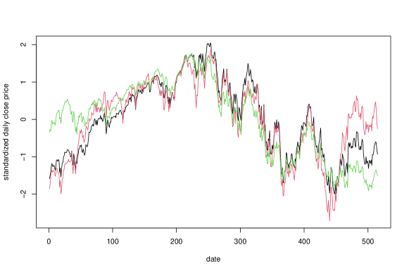
Figure 1: Plot of the standardized daily close price, from Jan-01-2021 to Jan-19-2023, of the 3 major stock market indices.

Table 7: Confidence intervals constructed for change point locations in the Real data example.

	$\alpha=0.01$		$\alpha=0.05$
$\widehat{\eta}$	Lower bound	Upper bound	Lower bound	Upper bound
April-07-2021	April-01-2021	April-12-2021	April-05-2021	April-09-2021
June-30-2021	June-23-2021	July-09-2021	June-25-2021	July-07-2021
Oct-19-2021	Oct-12-2021	Oct-26-2021	Oct-14-2021	Oct-22-2021
Jan-18-2021	Jan-12-2021	Jan-21-2021	Jan-13-2021	Jan-20-2021
April-25-2022	April-20-2022	April-28-2022	April-21-2022	April-27-2022
Oct-27-2022	Oct-24-2022	Nov-01-2022	Oct-25-2022	Oct-31-2022

The result of the implementation of NMP and ECP methods on the same dataset are {April-01-2021, July-01-2021, Oct-19-2021, Jan-14-2022, April-21-2022, Oct-26-2022} and {April-08-2021, June-25-2021, Oct-18-2021, Jan-18-2022, April-28-2022, Aug-24-2022, Oct-27-2022} respectively.

Appendix B Proof of Theorem 1

In this section, we present the proof of theorem Theorem 1.

Proof of Theorem 1.

For any $(s,e]\subseteq(0,T]$, let

$$\widetilde{f}^{(s,e]}_{t}(x)=\sqrt{\frac{e-t}{(e-s)(t-s)}}\sum_{l=s+1}^{t}f_{l}(x)-\sqrt{\frac{t-s}{(e-s)(e-t)}}\sum_{l=t+1}^{e}f_{l}(x),\ x\in\mathcal{X}.$$

For any $\widetilde{r}\in(\rho,T-\rho]$, we consider

$$\mathcal{A}((s,e],\rho,\lambda)=\bigg{\{}\max_{t=s+\rho+1}^{e-\rho}\sup_{x\in\mathbb{R}^{p}}|\widetilde{F}_{t,h}^{s,e}(x)-\widetilde{f}_{t}^{s,e}(x)|\leq\lambda\bigg{\}};$$

$$\mathcal{B}(\widetilde{r},\rho,\lambda)=\bigg{\{}\max_{N=\rho}^{T-\widetilde{r}}\sup_{x\in\mathbb{R}^{p}}\bigg{|}\frac{1}{\sqrt{N}}\sum_{t=\widetilde{r}+1}^{\widetilde{r}+N}F_{t,h}(x)-\frac{1}{\sqrt{N}}\sum_{t=\widetilde{r}+1}^{\widetilde{r}+N}f_{t}(x)\bigg{|}\leq\lambda\bigg{\}}\bigcup$$

$$\quad\quad\quad\quad\quad\ \ \bigg{\{}\max_{N=\rho}^{\widetilde{r}}\sup_{x\in\mathbb{R}^{p}}\bigg{|}\frac{1}{\sqrt{N}}\sum_{t=\widetilde{r}-N+1}^{\widetilde{r}}F_{t,h}(x)-\frac{1}{\sqrt{N}}\sum_{t=\widetilde{r}-N+1}^{\widetilde{r}}f_{t}(x)\bigg{|}\leq\lambda\bigg{\}}.$$

From Algorithm 1, we have that

$$\rho=\frac{\log(T)}{h^{p}}.$$

Therefore, Proposition 2 imply that with

$$\lambda=C_{\lambda}\bigg{(}2C\sqrt{\frac{\log T}{h^{p}}}+\frac{2C_{1}\sqrt{p}}{\sqrt{h^{p}}}+2C_{2}\sqrt{T}h^{r}.\bigg{)},$$ (17)

for some diverging sequence $C_{\lambda}$, it holds that

$$P\bigg{\{}\mathcal{A}^{c}((s,e],\rho,\lambda)\bigg{\}}\lesssim\frac{1}{T^{2}},$$

and,

$$P\bigg{\{}\mathcal{B}^{c}(\widetilde{r},\rho,\frac{\lambda}{2})\bigg{\}}\lesssim\frac{1}{T^{2}}.$$

Now, we notice that,

$$\sum_{k=1}^{\mathfrak{K}}\widetilde{n}_{k}=\sum_{k=1}^{\mathfrak{K}}(2^{k}-1)\leq\sum_{k=1}^{\mathfrak{K}}2^{k}\leq 2(2^{\lceil C_{\mathfrak{K}}(\log(T))\rceil}-1)=O(T).$$

In addition, there are $K=O(1)$ number of change points. In consequence, it follows that

$$P\bigg{\{}\mathcal{A}(\mathcal{I},\rho,\lambda)\text{ for all }\mathcal{I}\in\mathcal{J}\bigg{\}}\geq 1-\frac{1}{T},$$ (18)

$$P\bigg{\{}\mathcal{B}(s,\rho,\lambda)\cup\mathcal{B}(e,\rho,\lambda)\text{ for all }\mathcal{(}s,e]=\mathcal{I}\in\mathcal{J}\bigg{\}}\geq 1-\frac{1}{T},$$ (19)

$$P\bigg{\{}\mathcal{B}(\eta_{k},\rho,\lambda)\text{ for all }1\leq k\leq K\bigg{\}}\geq 1-\frac{1}{T}.$$ (20)

The rest of the argument is made by assuming the events in equations (18), (19) and (20) hold. By Remark 1, we have that on these events, it is satisfied that

$$\max_{t=s+\rho+1}^{e-\rho}||\widetilde{F}_{t,h}^{s,e}(x)-\widetilde{f}_{t}^{s,e}(x)||_{L_{2}}\leq\lambda.$$

Denote

$$\Upsilon_{k}=C\log(T)\bigg{(}T^{\frac{p}{2r+p}}\bigg{)}\kappa_{k}^{-2}\quad\text{and}\quad\Upsilon_{\max}=C\log(T)\bigg{(}T^{\frac{p}{2r+p}}\bigg{)}\kappa^{-2},$$

where $\kappa=\min\{\kappa_{1},\ldots,\kappa_{K}\}$. Since $\Upsilon_{k}$ is the desired localisation rate, by induction, it suffices to consider any generic interval $(s,e]\subseteq(0,T]$ that satisfies the following three conditions:

$$\eta_{m-1}\leq s\leq\eta_{m}\leq\ldots\leq\eta_{m+q}\leq e\leq\eta_{m+q+1},\quad q\geq-1;$$

$$\text{ either }\eta_{m}-s\leq\Upsilon_{m}\quad\text{or}\quad s-\eta_{m-1}\leq\Upsilon_{m-1};$$

$$\text{ either }\eta_{m+q+1}-e\leq\Upsilon_{m+q+1}\quad\text{or}\quad e-\eta_{m+q}\leq\Upsilon_{m+q}.$$

Here $q=-1$ indicates that there is no change point contained in $(s,e]$.

Denote

$$\Delta_{k}=\eta_{k-1}-\eta_{k}\text{ for }k=1,\ldots,K+1\quad\text{and}\quad\Delta=\min\{\Delta_{1},\ldots,\Delta_{K+1}\}.$$

Observe that since $\kappa_{k}>0$ for all $1\leq k\leq K$ and that $\Delta_{k}=\Theta(T)$, it holds that $\Upsilon_{\max}=o(\Delta)$. Therefore, it has to be the case that for any true change point $\eta_{m}\in(0,T]$, either $|\eta_{m}-s|\leq\Upsilon_{m}$ or $|\eta_{m}-s|\geq\Delta-\Upsilon_{\max}\geq\Theta(T)$. This means that $\min\{|\eta_{m}-e|,|\eta_{m}-s|\}\leq\Upsilon_{m}$ indicates that $\eta_{m}$ is a detected change point in the previous induction step, even if $\eta_{m}\in(s,e]$. We refer to $\eta_{m}\in(s,e]$ as an undetected change point if $\min\{\eta_{m}-s,\eta_{m}-e\}=\Theta(T)$. To complete the induction step, it suffices to show that MNSBS$((s,e],h,\tau)$
(i) will not detect any new change point in $(s,e]$ if all the change points in that interval have been previously detected, and
(ii) will find a point $D_{m*}^{\mathcal{I}^{*}}$ in $(s,e]$ such that $|\eta_{m}-D_{m*}^{\mathcal{I}^{*}}|\leq\Upsilon_{m}$ if there exists at least one undetected change point in $(s,e]$.

In order to accomplish this, we need the following series of steps.

Step 1. We first observe that if $\eta_{k}\in\{\eta_{k}\}_{k=1}^{K}$ is any change point in the functional time series, by Lemma 5, there exists a seeded interval $\mathcal{I}_{k}=(s_{k},e_{k}]$ containing exactly one change point $\eta_{k}$ such that

$$\min\{\eta_{k}-s_{k},e_{k}-\eta_{k}\}\geq\frac{1}{16}\zeta_{k},\quad\text{and}\quad\max\{\eta_{k}-s_{k},e_{k}-\eta_{k}\}\leq\zeta_{k}$$

where,

$$\zeta_{k}=\frac{9}{10}\min\{\eta_{k+1}-\eta_{k},\eta_{k}-\eta_{k-1}\}.$$

Even more, we notice that if $\eta_{k}\in(s,e]$ is any undetected change point in $(s,e]$. Then it must hold that

$$s-\eta_{k-1}\leq\Upsilon_{\max}.$$

Since $\Upsilon_{\max}=O(\log(T)T^{\frac{p}{2r+p}})$ and $O(\log^{a}(T))=o(T^{b})$ for any positive numbers $a$ and $b$, we have that $\Upsilon_{\max}=o(T)$. Moreover, $\eta_{k}-s_{k}\leq\zeta_{k}\leq\frac{9}{10}(\eta_{k}-\eta_{k-1})$, so that it holds that

$$s_{k}-\eta_{k-1}\geq\frac{1}{10}(\eta_{k}-\eta_{k-1})>\Upsilon_{\max}\geq s-\eta_{k-1}$$

and in consequence $s_{k}\geq s$. Similarly $e_{k}\leq e$. Therefore

$$\mathcal{I}_{k}=(s_{k},e_{k}]\subseteq(s,e].$$

Step 2. Consider the collection of intervals $\{\mathcal{I}_{k}=(s_{k},e_{k}]\}_{k=1}^{K}$ in Step 1. In this step, it is shown that for each $k\in\{1,\ldots,K\}$, it holds that

$$\max_{t=s_{k}+\rho}^{t=e_{k}-\rho}||\widetilde{F}_{t,h}^{(s_{k},e_{k}]}||_{L_{2}}\geq c_{1}\sqrt{T}\kappa_{k},$$ (21)

for some sufficient small constant $c_{1}$.

Let $k\in\{1,\ldots,K\}$. By Step 1, $\mathcal{I}_{k}$ contains exactly one change point $\eta_{k}$. Since $f_{t}$ is a one-dimensional population time series and there is only one change point in $\mathcal{I}_{k}=(s_{k},e_{k}]$, it holds that

$$f_{s_{k}+1}=...=f_{\eta_{k}}\neq f_{\eta_{k}+1}=...=f_{e_{k}}$$

which implies, for $s_{k}<t<\eta_{k}$

$$\widetilde{f}^{(s_{k},e_{k}]}_{t}= \sqrt{\frac{e_{k}-t}{(e_{k}-s_{k})(t-s_{k})}}\sum_{l=s_{k}+1}^{t}f_{\eta_{k}}-\sqrt{\frac{t-s_{k}}{(e_{k}-s_{k})(e_{k}-t)}}\sum_{l=t+1}^{\eta_{k}}f_{\eta_{k}}$$

$$- \sqrt{\frac{t-s_{k}}{(e_{k}-s_{k})(e_{k}-t)}}\sum_{l=\eta_{k}+1}^{e_{k}}f_{\eta_{k}+1}$$

$$= (t-s_{k})\sqrt{\frac{e_{k}-t}{(e_{k}-s_{k})(t-s_{k})}}f_{\eta_{k}}-(\eta_{k}-t)\sqrt{\frac{t-s_{k}}{(e_{k}-s_{k})(e_{k}-t)}}f_{\eta_{k}}$$

$$- (e_{k}-\eta_{k})\sqrt{\frac{t-s_{k}}{(e_{k}-s_{k})(e_{k}-t)}}f_{\eta_{k}+1}$$

$$= \sqrt{\frac{(t-s_{k})(e_{k}-t)}{(e_{k}-s_{k})}}f_{\eta_{k}}-(\eta_{k}-t)\sqrt{\frac{t-s_{k}}{(e_{k}-s_{k})(e_{k}-t)}}f_{\eta_{k}}$$

$$- (e_{k}-\eta_{k})\sqrt{\frac{t-s_{k}}{(e_{k}-s_{k})(e_{k}-t)}}f_{\eta_{k}+1}$$

$$= (e_{k}-t)\sqrt{\frac{t-s_{k}}{(e_{k}-t)(e_{k}-s_{k})}}f_{\eta_{k}}-(\eta_{k}-t)\sqrt{\frac{t-s_{k}}{(e_{k}-s_{k})(e_{k}-t)}}f_{\eta_{k}}$$

$$- (e_{k}-\eta_{k})\sqrt{\frac{t-s_{k}}{(e_{k}-s_{k})(e_{k}-t)}}f_{\eta_{k}+1}$$

$$= (e_{k}-\eta_{k})\sqrt{\frac{t-s_{k}}{(e_{k}-t)(e_{k}-s_{k})}}f_{\eta_{k}}-(e_{k}-\eta_{k})\sqrt{\frac{t-s_{k}}{(e_{k}-s_{k})(e_{k}-t)}}f_{\eta_{k}+1}$$

$$= (e_{k}-\eta_{k})\sqrt{\frac{t-s_{k}}{(e_{k}-t)(e_{k}-s_{k})}}(f_{\eta_{k}}-f_{\eta_{k}+1}).$$

Similarly, for $\eta_{k}\leq t\leq e_{k}$

$$f^{(s_{k},e_{k}]}_{t}=\sqrt{\frac{e_{k}-t}{(e_{k}-s_{k})(t-s_{k})}}(\eta_{k}-s_{k})(f_{\eta_{k}}-f_{\eta_{k}+1}).$$

Therefore,

$$\widetilde{f}^{(s_{k},e_{k}]}_{t}=\begin{cases}\sqrt{\frac{t-s_{k}}{(e_{k}-s_{k})(e_{k}-t)}}(e_{k}-\eta_{k})(f_{\eta_{k}}-f_{\eta_{k}+1}),&s_{k}<t<\eta_{k};\\ \sqrt{\frac{e_{k}-t}{(e_{k}-s_{k})(t-s_{k})}}(\eta_{k}-s_{k})(f_{\eta_{k}}-f_{\eta_{k}+1}),&\eta_{k}\leq t\leq e_{k}.\end{cases}$$ (22)

Since $\Delta=\Theta(T)$, $\rho=O(\log(T)T^{\frac{p}{2r+p}})$ and $\log^{a}(T)=o(T^{b})$ for any positive numbers $a$ and $b,$ we have that

$$\min\{\eta_{k}-s_{k},e_{k}-\eta_{k}\}\geq\frac{1}{16}\zeta_{k}\geq\frac{3}{4}c_{2}T>\rho,$$ (23)

so that $\eta_{k}\in[s_{k}+\rho,e_{k}-\rho]$. Then, from (22), (23) and the fact that $|e_{k}-s_{k}|<T$ and $|\eta_{k}-s_{k}|<T$,

$$||\widetilde{f}^{(s_{k},e_{k}]}_{\eta_{k}}||_{L_{2}}=\sqrt{\frac{e_{k}-\eta_{k}}{(e_{k}-s_{k})(\eta_{k}-s_{k})}}(\eta_{k}-s_{k})||f_{\eta_{k}}-f_{\eta_{k}+1}||_{L_{2}}\geq c_{2}\sqrt{T}\frac{3}{4}\kappa_{k}.$$ (24)

Therefore, it holds that

$$\max_{t=s_{k}+\rho}^{t=e_{k}-\rho}||\widetilde{F}^{(s_{k},e_{k}]}_{t,h}||_{L_{2}}\geq ||\widetilde{F}^{(s_{k},e_{k}]}_{\eta_{k},h}||_{L_{2}}$$

$$\geq ||\widetilde{f}^{(s_{k},e_{k}]}_{\eta_{k}}||_{L_{2}}-\lambda$$

$$\geq c_{2}\frac{3}{4}\sqrt{T}\kappa_{k}-\lambda,$$

where the first inequality follows from the fact that $\eta_{k}\in[s_{k}+\rho,e_{k}-\rho]$, the second inequality follows from the good event in (18) and Remark 2, and the last inequality follows from (24).
Next, we observe that $\log^{\frac{1}{2}}(T)\sqrt{\frac{1}{h^{p}}}=o(\sqrt{T^{\frac{2r+p}{p}}})O(\sqrt{T^{\frac{p}{2r+p}}})=o(\sqrt{T})$, $\rho<c_{2}T$, and $h^{r}=o(1)$. In consequence, since $\kappa_{k}$ is a positive constant, by the upper bound of $\lambda$ on Equation 17, for sufficiently large $T$, it holds that

$$\frac{c_{2}}{4}\sqrt{T}\kappa_{k}\geq\lambda.$$

Therefore,

$$\max_{t=s_{k}+\rho}^{t=e_{k}-\rho}||\widetilde{F}^{(s_{k},e_{k}]}_{t,h}||_{L_{2}}\geq\frac{c_{2}}{2}\sqrt{T}\kappa_{k}.$$

Therefore Equation 21 holds with $c_{1}=\frac{c_{2}}{2}.$

Step 3. In this step, it is shown that SBS$((s,e],h,\tau)$ can consistently detect or reject the existence of undetected change points within $(s,e]$.

Suppose $\eta_{k}\in(s,e]$ is any undetected change point. Then by the second half of Step 1, $\mathcal{I}_{k}\subseteq(s,e]$. Therefore

$$A_{\mathcal{I}^{*}}\geq\max_{t=s_{k}+\rho}^{t=e_{k}-\rho}||\widetilde{F}_{t,h}^{(s_{k},e_{k}]}||_{L_{2}}\geq c_{1}\sqrt{T}\kappa_{k}>\tau,$$

where the second inequality follows from Equation 21, and the last inequality follows from the fact that, $\log^{a}(T)=o(T^{b})$ for any positive numbers $a$ and $b$ implies $\tau=C_{\tau}\bigg{(}\log(T)\sqrt{\frac{1}{h^{p}}}\bigg{)}=o(\sqrt{T})$.

Suppose there does not exist any undetected change point in $(s,e]$. Then for any $\mathcal{I}=(\alpha,\beta]\subseteq(s,e]$, one of the following situations must hold,

• There is no change point within $(\alpha,\beta]$;

• there exists only one change point $\eta_{k}$ within $(\alpha,\beta]$ and $\min\{\eta_{k}-\alpha,\beta-\eta_{k}\}\leq\Upsilon_{k}$;

• there exist two change points $\eta_{k},\eta_{k+1}$ within $(\alpha,\beta]$ and

  $$\eta_{k}-\alpha\leq\Upsilon_{k}\quad\text{and}\quad\beta-\eta_{k+1}\leq\Upsilon_{k+1}.$$

Observe that if (a) holds, then we have

$$\max_{\alpha+\rho<t<\beta-\rho}||\widetilde{F}_{t,h}^{(\alpha,\beta]}||_{L_{2}}\leq\max_{\alpha+\rho<t<\beta-\rho}||\widetilde{f}_{t}^{(\alpha,\beta]}||_{L_{2}}+\lambda=\lambda\text{. }$$

Cases (b) and (c) can be dealt with using similar arguments. We will only work on (c) here. It follows that, in the good event in Equation 18,

$$\max_{\alpha+\rho<t<\beta-\rho}||\widetilde{F}_{t,h}^{(\alpha,\beta]}||_{L_{2}} \leq\max_{\alpha<t<\beta}||\widetilde{f}_{t}^{(\alpha,\beta]}||_{L_{2}}+\lambda$$ (25)

$$\leq\sqrt{e-\eta_{k}}\kappa_{k+1}+\sqrt{\eta_{k}-s}\kappa_{k}+\lambda$$ (26)

$$\leq 2\sqrt{C}\log^{\frac{1}{2}}(T)\sqrt{T^{\frac{p}{2r+p}}}+\lambda$$ (27)

where the second inequality is followed by Lemma 7. Therefore in the good event in Equation 18, for any $\mathcal{I}=(\alpha,\beta]\subseteq(s,e]$, it holds that

$$A_{\mathcal{I}}=\max_{t=\alpha+\rho}^{\beta-\rho}||\widetilde{F}_{t,h}^{(\alpha,\beta]}||_{L_{2}}\leq 2\sqrt{C}\log^{\frac{1}{2}}(T)\sqrt{T^{\frac{p}{2r+p}}}+\lambda,$$

Then,

$$2\sqrt{C}\log^{\frac{1}{2}}(T)\sqrt{1+T^{\frac{p}{2r+p}}}+\lambda_{\mathcal{A}}$$

$$= 2\sqrt{C}\log^{\frac{1}{2}}(T)\sqrt{\frac{1}{h^{p}}+1}+2C\sqrt{\frac{\log T}{h^{p}}}+\frac{2C_{1}\sqrt{p}}{\sqrt{h^{p}}}+2C_{2}\sqrt{T}h^{r}.$$

We observe that $\sqrt{\frac{\log(T)}{h^{p}}}=O\Big{(}\log(T)^{1/2}\sqrt{\frac{1}{h^{p}}}\Big{)}$. Moreover,

$$\sqrt{T}h^{r}=\sqrt{T}\Big{(}\frac{1}{T}\Big{)}^{\frac{r}{2r+p}}\leq\Big{(}T^{\frac{1}{2}-\frac{r}{2r+p}}\Big{)},$$

and given that,

$$\frac{1}{2}-\frac{r}{2r+p}=\frac{p}{2(2r+p)}$$

we get,

$$\sqrt{T}h^{r}=o\Big{(}\log^{\frac{1}{2}}(T)\sqrt{\frac{1}{h^{p}}}\Big{)}.$$

Therefore, by the choice of $\tau$, we will always correctly reject the existence of undetected change points, since

$$2\sqrt{C}\log^{\frac{1}{2}}(T)\sqrt{T^{\frac{p}{2r+p}}}+\lambda\leq\tau.$$

Thus, by the choice of $\tau$, it holds that with sufficiently large constant $C_{\tau}$,

$$A_{m}^{\mathcal{I}}\leq\tau\quad\text{for all }\quad\mathcal{I}\subseteq(s,e].$$ (28)

As a result, MNSBS$((s,e],h,\tau)$ will correctly reject if $(s,e]$ contains no undetected change points.
 
Step 4. Assume that there exists an undetected change point $\eta_{\widetilde{k}}\in(s,e]$ such that

$$\min\{\eta_{\widetilde{k}}-s,\eta_{\widetilde{k}}-e\}=\Theta(T).$$

Let $\mathcal{I}^{*}$ be defined as in MNSBS $((s,e],h,\tau)$ with

$$\mathcal{I}^{*}=(\alpha^{*},\beta^{*}].$$

To complete the induction, it suffices to show that, there exists a change point $\eta_{k}\in(s,e]$ such that $\min\{\eta_{k}-s,\eta_{k}-e\}=\Theta(T)$ and $|b_{\mathcal{I}^{*}}-\eta_{k}|\leq\Upsilon_{k}$. To this end, we consider the collection of change points of $\{f_{t}\}_{t\in(\alpha^{*},\beta^{*}]}$ We are to ensure that the assumptions of Lemma 12 are satisfied. In the following, $\lambda$ is used in Lemma 12. Then Equation 74 and Equation 75 are directly consequence of Equation 18, Equation 19, Equation 20. By Step 1 with $\mathcal{I}_{k}=(s_{k},e_{k}]$, it holds that

$$\min\{\eta_{k}-s_{k},e_{k}-\eta_{k}\}\geq\frac{1}{16}\zeta_{k}\geq c_{2}T,$$

Therefore for all $k\in\{\widetilde{k}:\min\{\eta_{\widetilde{k}}-s,e-\eta_{\widetilde{k}}\}\geq c_{2}T\}$,

$$\max_{t=\alpha^{*}+\rho}^{t=\beta^{*}-\rho}||\widetilde{F}_{t,h}^{(\alpha^{*},\beta^{*}]}||_{L_{2}}\geq\max_{t=s_{k}+\rho}^{t=e_{k}-\rho}||\widetilde{F}_{t,h}^{(s_{k},e_{k}]}||_{L_{2}}\geq c_{1}\sqrt{T}\kappa_{k},$$

where the last inequality follows from Equation 21. Therefore (76) holds in Lemma 12. Finally, Equation 77 is a direct consequence of the choices that

$$h=C_{h}(T)^{\frac{-1}{2r+d}}\quad\text{and}\quad\rho=\frac{\log(T)}{nh^{d}}.$$

Thus, all the conditions in Lemma 12 are met. So that, there exists a change point $\eta_{k}$ of $\{f_{t}\}_{t\in\mathcal{I}^{*}}$, satisfying

$$\min\{\beta^{*}-\eta_{k},\eta_{k}-\alpha^{*}\}>cT,$$ (29)

and

$$|b_{\mathcal{I}^{*}}-\eta_{k}|\leq\max\{C_{3}\lambda^{2}\kappa_{k}^{-2},\rho\}\leq C_{4}\log(T)\bigg{(}\frac{1}{h^{p}}+Th^{2r}\bigg{)}\kappa_{k}^{-2}$$

$$\leq C\log(T)\bigg{(}T^{\frac{p}{2r+p}}\bigg{)}\kappa_{k}^{-2}$$

for sufficiently large constant $C$, where we have followed the same line of arguments as for the conclusion of (28). Observe that
i) The change points of $\{f_{t}\}_{t\in\mathcal{I}^{*}}$ belong to $(s,e]\cap\{\eta_{k}\}_{k=1}^{K}$; and
ii) Equation 29 and $(\alpha^{*},\beta^{*}]\subseteq(s,e]$ imply that

$$\min\{e-\eta_{k},\eta_{k}-s\}>cT\geq\Upsilon_{\max}.$$

As discussed in the argument before Step 1, this implies that $\eta_{k}$ must be an undetected change point of $\{f_{t}\}_{t\in\mathcal{I}^{*}}$. ∎

Appendix C Proof of Theorem 2

In this section, we present the proof of theorem Theorem 2.

Proof of Theorem 2.

Uniform tightness of $\kappa_{k}^{2+\frac{p}{r}}\Big{|}\widetilde{\eta}_{k}-\eta_{k}\Big{|}$. Here we show a.1 and b.1. For this purpose, we will follow a series of steps. On step 1, we rewrite (8) in order to derive a uniform bound. Step 2 analyses the lower bound while Step 3 the upper bound.
Step 1: Denote $\widetilde{r}=\widetilde{\eta}_{k}-\eta_{k}$. Without loss of generality, suppose $\widetilde{r}\geq 0$. Since $\widetilde{\eta}_{k}=\eta_{k}+\widetilde{r}$, defined in (8), is the minimizer of $\widehat{Q}_{k}(\eta)$, it follows that

$$\widehat{Q}_{k}(\eta_{k}+\widetilde{r})-\widehat{Q}_{k}(\eta_{k})\leq 0.$$

Let

$$Q^{*}(\eta)=\sum_{t=s_{k}+1}^{\eta}||F_{t,h_{2}}-f_{(s_{k},\eta_{k}]}\ast\mathcal{K}_{h_{2}}||_{L_{2}}^{2}+\sum_{t=\eta+1}^{e_{k}}||F_{t,h_{2}}-f_{(\eta_{k},e_{k}]}\ast\mathcal{K}_{h_{2}}||_{L_{2}}^{2},$$ (30)

where,

$$f_{(s_{k},\eta_{k}]}=\frac{1}{\eta_{k}-s_{k}}\sum_{i=s_{k}+1}^{\eta_{k}}f_{i},\ f_{(\eta_{k},e_{k}]}=\frac{1}{e_{k}-\eta_{k}}\sum_{i=\eta_{k}+1}^{e_{k}}f_{i}.$$ (31)

Observe that,

$$Q^{*}(\eta_{k}+\widetilde{r})-Q^{*}(\eta_{k})\leq \widehat{Q}_{k}(\eta_{k})-\widehat{Q}_{k}(\eta_{k}+\widetilde{r})-Q^{*}(\eta_{k})+Q^{*}(\eta_{k}+\widetilde{r}).$$ (32)

If $\widetilde{r}\leq 1/\kappa_{k}^{2+\frac{p}{r}}$, then there is nothing to show. So for the rest of the argument, for contradiction, assume that

$$\widetilde{r}\geq\frac{1}{\kappa_{k}^{2+\frac{p}{r}}}.$$ (33)

Step 2: Finding a lower bound. In this step, we will find a lower bound of the inequality (32). To this end, we observe that,

$$Q^{*}(\eta_{k}+\widetilde{r})-Q^{*}(\eta_{k})= \sum_{t=\eta_{k}+1}^{\eta_{k}+\widetilde{r}}||F_{t,{h_{2}}}-f_{(s_{k},\eta_{k}]}\ast\mathcal{K}_{{h_{2}}}||_{L_{2}}^{2}-\sum_{t=\eta_{k}+1}^{\eta_{k}+\widetilde{r}}||F_{t,{h_{2}}}-f_{(\eta_{k},e_{k}]}\ast\mathcal{K}_{h_{2}}||_{L_{2}}^{2}$$

$$= \sum_{t=\eta_{k}+1}^{\eta_{k}+\widetilde{r}}||f_{(s_{k},\eta_{k}]}\ast\mathcal{K}_{{h_{2}}}-f_{(\eta_{k},e_{k}]}\ast\mathcal{K}_{h_{2}}||_{L_{2}}^{2}$$

$$-2\sum_{t=\eta_{k}+1}^{\eta_{k}+\widetilde{r}}\langle f_{(s_{k},\eta_{k}]}\ast\mathcal{K}_{{h_{2}}}-f_{(\eta_{k},e_{k}]}\ast\mathcal{K}_{h_{2}},F_{t,{h_{2}}}-f_{(\eta_{k},e_{k}]}\ast\mathcal{K}_{h_{2}}\rangle_{L_{2}}$$

$$= \sum_{t=\eta_{k}+1}^{\eta_{k}+\widetilde{r}}\frac{1}{2}||f_{(s_{k},\eta_{k}]}-f_{(\eta_{k},e_{k}]}||_{L_{2}}^{2}-2||f_{(s_{k},\eta_{k}]}\ast\mathcal{K}_{{h_{2}}}-f_{(s_{k},\eta_{k}]}+f_{(\eta_{k},e_{k}]}\ast\mathcal{K}_{h_{2}}-f_{(\eta_{k},e_{k}]}||_{L_{2}}^{2}$$

$$-2\sum_{t=\eta_{k}+1}^{\eta_{k}+\widetilde{r}}\langle f_{(s_{k},\eta_{k}]}\ast\mathcal{K}_{{h_{2}}}-f_{(\eta_{k},e_{k}]}\ast\mathcal{K}_{h_{2}},F_{t,{h_{2}}}-f_{(\eta_{k},e_{k}]}\ast\mathcal{K}_{h_{2}}\rangle_{L_{2}}$$

$$\geq \frac{1}{2}\widetilde{r}\kappa_{k}^{2}-2\sum_{t=\eta_{k}+1}^{\eta_{k}+\widetilde{r}}||f_{(s_{k},\eta_{k}]}\ast\mathcal{K}_{{h_{2}}}-f_{(s_{k},\eta_{k}]}+f_{(\eta_{k},e_{k}]}\ast\mathcal{K}_{h_{2}}-f_{(\eta_{k},e_{k}]}||_{L_{2}}^{2}$$

$$-2\sum_{t=\eta_{k}+1}^{\eta_{k}+\widetilde{r}}\langle f_{(s_{k},\eta_{k}]}\ast\mathcal{K}_{{h_{2}}}-f_{(\eta_{k},e_{k}]}\ast\mathcal{K}_{h_{2}},F_{t,{h_{2}}}-f_{(\eta_{k},e_{k}]}\ast\mathcal{K}_{h_{2}}\rangle_{L_{2}}$$

We consider,

$$I_{1}:=2\sum_{t=\eta_{k}+1}^{\eta_{k}+\widetilde{r}}||f_{(s_{k},\eta_{k}]}\ast\mathcal{K}_{{h_{2}}}-f_{(s_{k},\eta_{k}]}+f_{(\eta_{k},e_{k}]}\ast\mathcal{K}_{h_{2}}-f_{(\eta_{k},e_{k}]}||_{L_{2}}^{2},\ \text{and,}$$

$$I_{2}:=2\sum_{t=\eta_{k}+1}^{\eta_{k}+\widetilde{r}}\langle f_{(s_{k},\eta_{k}]}\ast\mathcal{K}_{{h_{2}}}-f_{(\eta_{k},e_{k}]}\ast\mathcal{K}_{h_{2}},F_{t,{h_{2}}}-f_{(\eta_{k},e_{k}]}\ast\mathcal{K}_{h_{2}}\rangle_{L_{2}}.$$

From above, we have that,

$$Q^{*}(\eta_{k}+\widetilde{r})-Q^{*}(\eta_{k})\geq \frac{1}{2}\widetilde{r}\kappa_{k}^{2}-I_{1}-I_{2}.$$

We now analyze the order of magnitude of term $I_{1}$. Then, we get a lower bound for the term $-I_{1}.$ In fact $I_{1}$, has an upper bound of the form $o_{p}(\widetilde{r}k^{\frac{p}{r}+2})$, where we use that $||f_{\eta_{k}}\ast\mathcal{K}_{{h_{2}}}-f_{\eta_{k}}||_{L_{2}}=o(1)$ and $||f_{\eta_{k+1}}\ast\mathcal{K}_{{h_{2}}}-f_{\eta_{k+1}}||_{L_{2}}=o(1)$. For the term $I_{2}$, we consider the random variable,

$$Y_{i}=\frac{\langle f_{[s_{k}+1,\eta_{k}]}\ast\mathcal{K}_{{h_{2}}}-f_{[\eta_{k}+1,e_{k}]}\ast\mathcal{K}_{h_{2}},F_{t,{h_{2}}}-f_{[\eta_{k}+1,e_{k}]}\ast\mathcal{K}_{h_{2}}\rangle_{L_{2}}}{\kappa_{k}\mathbb{E}(||F_{t,{h_{2}}}-f_{\eta_{k+1}}\ast\mathcal{K}_{h_{2}}||_{L^{2}}^{3})^{1/3}}.$$

In order to use Lemma 3, we need to bound $\mathbb{E}(|Y_{i}|^{3}).$ For this, first we use Cauchy Schwartz inequality,

$$\mathbb{E}(|Y_{i}|^{3})\leq \frac{(||(f_{\eta_{k}+1}-f_{\eta_{k}})\ast\mathcal{K}_{h_{2}}||_{L^{2}})^{3}\mathbb{E}(||F_{t,{h_{2}}}-f_{\eta_{k+1}}\ast\mathcal{K}_{h_{2}}||_{L^{2}}^{3})}{\kappa_{k}^{3}\mathbb{E}(||F_{t,{h_{2}}}-f_{\eta_{k+1}}\ast\mathcal{K}_{h_{2}}||_{L^{2}}^{3})}$$

then, by Minkowski’s inequality,

$$||(f_{\eta_{k}+1}-f_{\eta_{k}})\ast\mathcal{K}_{h_{2}}||_{L^{2}}= \Big{|}\Big{|}\int_{\mathbb{R}^{p}}(f_{\eta_{k}+1}-f_{\eta_{k}})(\cdot-y)\mathcal{K}_{h_{2}}(y)dy\Big{|}\Big{|}_{L_{2}}$$

$$\leq \int_{\mathbb{R}^{p}}\Big{|}\Big{|}(f_{\eta_{k}+1}-f_{\eta_{k}})(\cdot-y)\mathcal{K}_{h_{2}}(y)\Big{|}\Big{|}_{L_{2}}dy$$

$$= \Big{(}\int_{\mathbb{R}^{p}}|\mathcal{K}_{h_{2}}(y)|dy\Big{)}\Big{|}\Big{|}(f_{\eta_{k}+1}-f_{\eta_{k}})(\cdot-y)\Big{|}\Big{|}_{L_{2}}$$

$$= ||f_{\eta_{k}+1}-f_{\eta_{k}}||_{L^{2}}||\mathcal{K}_{h_{2}}||_{L^{1}}.$$

Therefore, by 2, we have

$$\frac{(||(f_{\eta_{k}+1}-f_{\eta_{k}})\ast\mathcal{K}_{h_{2}}||_{L^{2}})^{3}\mathbb{E}(||F_{t,{h_{2}}}-f_{\eta_{k+1}}\ast\mathcal{K}_{h_{2}}||_{L^{2}}^{3})}{\kappa_{k}^{3}\mathbb{E}(||F_{t,{h_{2}}}-f_{\eta_{k+1}}\ast\mathcal{K}_{h_{2}}||_{L^{2}}^{3})}$$

$$\leq \frac{(||f_{\eta_{k}+1}-f_{\eta_{k}}||_{L^{2}}||\mathcal{K}_{h_{2}}||_{L^{1}})^{3}\mathbb{E}(||F_{t,{h_{2}}}-f_{\eta_{k+1}}\ast\mathcal{K}_{h_{2}}||_{L^{2}}^{3})}{\kappa_{k}^{3}\mathbb{E}(||F_{t,{h_{2}}}-f_{\eta_{k+1}}\ast\mathcal{K}_{h_{2}}||_{L^{2}}^{3})}$$

$$\leq C_{K}.$$

for any $t\in{(\eta_{k},e_{k}]}$. Moreover, we have that

$$\begin{array}[]{lll}\mathbb{E}(||F_{t,h_{2}}-f_{\eta_{k+1}}\ast\mathcal{K}_{h_{2}}||_{L^{2}}^{3})^{\frac{1}{3}}&=&\Big{(}\int\Big{(}\int(\mathcal{K}_{h_{2}}(x-z)-\mathbb{E}(\mathcal{K}_{h_{2}}(x-X_{t})))^{2}dx\Big{)}^{\frac{3}{2}}f_{t}(z)dz\Big{)}^{1/3}\\ &\leq&\Big{(}\int\Big{(}\int(\mathcal{K}_{h_{2}}(x-z))^{2}dx\Big{)}^{\frac{3}{2}}f_{t}(z)dz\Big{)}^{\frac{1}{3}}\\ &=&\frac{1}{\kappa^{p/2r}}.\end{array}$$ (34)

Therefore, by Lemma 3, we have that $I_{2}=o_{p}\Big{(}\sqrt{\widetilde{r}}\kappa_{k}\kappa_{k}^{-\frac{p}{2r}}(\log(\widetilde{r}\kappa_{k}^{\frac{p}{r}+2})+1)\Big{)}.$ Thus,

$$Q^{*}(\eta_{k}+\widetilde{r})-Q^{*}(\eta_{k})\geq \frac{1}{2}\widetilde{r}\kappa_{k}^{2}-O_{p}\Big{(}\sqrt{\widetilde{r}}\kappa_{k}\kappa_{k}^{-\frac{p}{2r}}(\log(\widetilde{r}\kappa_{k}^{\frac{p}{r}+2})+1)\Big{)}-o_{p}(\widetilde{r}\kappa_{k}^{\frac{p}{r}+2}).$$ (35)

Step 3: Finding an upper bound. Now, we proceeded to get an upper bound of (32). This is, an upper bound of the following expression,

$$\widehat{Q}_{k}(\eta_{k})-\widehat{Q}_{k}(\eta_{k}+\widetilde{r})-Q^{*}(\eta_{k})+Q^{*}(\eta_{k}+\widetilde{r}).$$ (36)

Observe that, this expression can be written as,

$$\widehat{Q}_{k}(\eta_{k})-\widehat{Q}_{k}(\eta_{k}+\widetilde{r})-Q^{*}(\eta_{k})+Q^{*}(\eta_{k}+\widetilde{r})$$

$$= -\sum_{t=\eta_{k}+1}^{\eta_{k}+\widetilde{r}}||F_{t,{h_{1}}}-F_{(s_{k},\eta_{k}],{h_{1}}}||_{L_{2}}^{2}+\sum_{t=\eta_{k}+1}^{\eta_{k}+\widetilde{r}}||F_{t,{h_{1}}}-F_{(\eta_{k},e_{k}],{h_{1}}}||_{L_{2}}^{2}$$

$$+\sum_{t=\eta_{k}+1}^{\eta_{k}+\widetilde{r}}||F_{t,{h_{2}}}-f_{(s_{k},\eta_{k}]}\ast\mathcal{K}_{{h_{2}}}||_{L_{2}}^{2}-\sum_{t=\eta_{k}+1}^{\eta_{k}+\widetilde{r}}||F_{t,{h_{2}}}-f_{(\eta_{k},e_{k}]}\ast\mathcal{K}_{h_{2}}||_{L_{2}}^{2}$$

So that,

$$\widehat{Q}_{k}(\eta_{k})-\widehat{Q}_{k}(\eta_{k}+\widetilde{r})-Q^{*}(\eta_{k})+Q^{*}(\eta_{k}+\widetilde{r})=U_{1}+U_{2},$$

where,

$$U_{1}=\sum_{t=\eta_{k}+1}^{\eta_{k}+\widetilde{r}}||F_{t,{h_{2}}}-f_{(s_{k},\eta_{k}]}\ast\mathcal{K}_{{h_{2}}}||_{L_{2}}^{2}-\sum_{t=\eta_{k}+1}^{\eta_{k}+\widetilde{r}}||F_{t,{h_{1}}}-F_{(s_{k},\eta_{k}],{h_{1}}}||_{L_{2}}^{2},\ \text{and,}$$

$$U_{2}=\sum_{t=\eta_{k}+1}^{\eta_{k}+\widetilde{r}}||F_{t,{h_{1}}}-F_{(\eta_{k},e_{k}],{h_{1}}}||_{L_{2}}^{2}-\sum_{t=\eta_{k}+1}^{\eta_{k}+\widetilde{r}}||F_{t,{h_{2}}}-f_{(\eta_{k},e_{k}]}\ast\mathcal{K}_{h_{2}}||_{L_{2}}^{2}.$$

Now, we analyze each of the terms above. For $U_{1},$ observe that

$$\sum_{t=\eta_{k}+1}^{\eta_{k}+\widetilde{r}}||F_{t,{h_{2}}}-f_{(s_{k},\eta_{k}]}\ast\mathcal{K}_{{h_{2}}}||_{L_{2}}^{2}-\sum_{t=\eta_{k}+1}^{\eta_{k}+\widetilde{r}}||F_{t,{h_{1}}}-F_{(s_{k},\eta_{k}],{h_{1}}}||_{L_{2}}^{2}$$

$$= \sum_{t=\eta_{k}+1}^{\eta_{k}+\widetilde{r}}||F_{t,{h_{2}}}-f_{(s_{k},\eta_{k}]}\ast\mathcal{K}_{{h_{2}}}||_{L_{2}}^{2}-\sum_{t=\eta_{k}+1}^{\eta_{k}+\widetilde{r}}||F_{t,{h_{2}}}-F_{(s_{k},\eta_{k}],{h_{2}}}||_{L_{2}}^{2}$$

$$+ \sum_{t=\eta_{k}+1}^{\eta_{k}+\widetilde{r}}||F_{t,{h_{2}}}-F_{(s_{k},\eta_{k}],{h_{2}}}||_{L_{2}}^{2}-\sum_{t=\eta_{k}+1}^{\eta_{k}+\widetilde{r}}||F_{t,{h_{1}}}-F_{(s_{k},\eta_{k}],{h_{1}}}||_{L_{2}}^{2}$$

$$= I_{3}+I_{4},$$

where,

$$I_{3}=\sum_{t=\eta_{k}+1}^{\eta_{k}+\widetilde{r}}||F_{t,{h_{2}}}-f_{(s_{k},\eta_{k}]}\ast\mathcal{K}_{{h_{2}}}||_{L_{2}}^{2}-\sum_{t=\eta_{k}+1}^{\eta_{k}+\widetilde{r}}||F_{t,{h_{2}}}-F_{(s_{k},\eta_{k}],{h_{2}}}||_{L_{2}}^{2},\ \text{and,}$$

$$I_{4}=\sum_{t=\eta_{k}+1}^{\eta_{k}+\widetilde{r}}||F_{t,{h_{2}}}-F_{(s_{k},\eta_{k}],{h_{2}}}||_{L_{2}}^{2}-\sum_{t=\eta_{k}+1}^{\eta_{k}+\widetilde{r}}||F_{t,{h_{1}}}-F_{(s_{k},\eta_{k}],{h_{1}}}||_{L_{2}}^{2}.$$

To analyze $I_{3},$ we rewrite it as follow,

$$I_{3}= \sum_{t=\eta_{k}+1}^{\eta_{k}+\widetilde{r}}||f_{(s_{k},\eta_{k}]}\ast\mathcal{K}_{{h_{2}}}-F_{(s_{k},\eta_{k}],{h_{2}}}||_{L_{2}}^{2}-2\sum_{t=\eta_{k}+1}^{\eta_{k}+\widetilde{r}}\langle f_{(s_{k},\eta_{k}]}\ast\mathcal{K}_{{h_{2}}}-F_{(s_{k},\eta_{k}],{h_{2}}},F_{t,{h_{2}}}-f_{(s_{k},\eta_{k}]}\ast\mathcal{K}_{{h_{2}}}\rangle_{L_{2}}$$

$$= I_{3,1}+I_{3,2},$$

where,

$$I_{3,1}=\sum_{t=\eta_{k}+1}^{\eta_{k}+\widetilde{r}}||f_{(s_{k},\eta_{k}]}\ast\mathcal{K}_{{h_{2}}}-F_{(s_{k},\eta_{k}],{h_{2}}}||_{L_{2}}^{2},\ \text{and,}$$

$$I_{3,2}=-2\sum_{t=\eta_{k}+1}^{\eta_{k}+\widetilde{r}}\langle f_{(s_{k},\eta_{k}]}\ast\mathcal{K}_{{h_{2}}}-F_{(s_{k},\eta_{k}],{h_{2}}},F_{t,{h_{2}}}-f_{(s_{k},\eta_{k}]}\ast\mathcal{K}_{{h_{2}}}\rangle_{L_{2}}.$$

Now, we will get an upper bound for each of the terms above. The term $I_{3,1}=O_{p}\Big{(}\widetilde{r}\frac{1}{T}\frac{\log(T)}{\kappa_{k}^{\frac{p}{r}}}\Big{)}$, which is followed by the use of Remark 1 and $\Delta=\Theta(T)$. Even more, by 4, we get

$$I_{3,1}=o_{p}(\widetilde{r}\kappa_{k}^{\frac{p}{r}+2}).$$ (37)

For the term $I_{3,2}$, by Cauchy Schwartz inequality and triangle inequality,

$$\langle f_{(s_{k},\eta_{k}]}\ast\mathcal{K}_{\kappa}-F_{(s_{k},\eta_{k}],\kappa},F_{t,{h_{2}}}-f_{(s_{k},\eta_{k}]}\ast\mathcal{K}_{{h_{2}}}\rangle_{L_{2}}$$

$$\leq||f_{(s_{k},\eta_{k}]}\ast\mathcal{K}_{{h_{2}}}-F_{(s_{k},\eta_{k}],{h_{2}}}||_{L_{2}}||F_{t,{h_{2}}}-f_{(s_{k},\eta_{k}]}\ast\mathcal{K}_{{h_{2}}}||_{L_{2}}$$

$$\leq||f_{(s_{k},\eta_{k}]}\ast\mathcal{K}_{{h_{2}}}-F_{(s_{k},\eta_{k}],{h_{2}}}||_{L_{2}}\Big{(}||F_{t,{h_{2}}}-f_{[\eta_{k}+1,e_{k}]}\ast\mathcal{K}_{{h_{2}}}||_{L_{2}}+||f_{[\eta_{k}+1,e_{k}]}\ast\mathcal{K}_{{h_{2}}}-f_{[s_{k}+1,\eta_{k}]}\ast\mathcal{K}_{{h_{2}}}||_{L_{2}}\Big{)}$$

for any $t\in{(\eta_{k},\eta_{k}+\widetilde{r}]}$. By the Remark 1, and the fact that $\Delta=\Theta(T)$, we have that

$$||f_{(s_{k},\eta_{k}]}\ast\mathcal{K}_{{h_{2}}}-F_{(s_{k},\eta_{k}],{h_{2}}}||_{L_{2}}=O_{p}\Big{(}\frac{1}{\sqrt{T}}\sqrt{\frac{\log(T)}{\kappa_{k}^{\frac{p}{r}}}}\Big{)}$$

and using basic properties of integrals $||f_{[\eta_{k}+1,e_{k}]}\ast\mathcal{K}_{h_{2}}-f_{[s_{k}+1,\eta_{k}]}\ast\mathcal{K}_{h_{2}}||_{L_{2}}=O(\kappa_{k}).$ Therefore,

$$I_{3,2} \leq O_{p}\Big{(}\frac{1}{\sqrt{T}}\sqrt{\frac{\log(T)}{\kappa_{k}^{\frac{p}{r}}}}\Big{)}\Big{(}O(\widetilde{r}\kappa_{k})+\sum_{t=\eta_{k}+1}^{\eta_{k}+\widetilde{r}}||F_{t,{h_{2}}}-f_{[\eta_{k}+1,e_{k}]}\ast\mathcal{K}_{{h_{2}}}||_{L_{2}}\Big{)}$$

Now, we need to get a bound of the magnitude of

$$\sum_{t=\eta_{k}+1}^{\eta_{k}+\widetilde{r}}||F_{t,{h_{2}}}-f_{[\eta_{k}+1,e_{k}]}\ast\mathcal{K}_{{h_{2}}}||_{L_{2}},$$

in order to get an upper for $I_{3,2}.$ This is done similarly to $I_{2}.$ We consider the random variable

$$\widetilde{Y}_{i}=\frac{\langle F_{t,{h_{2}}}-f_{(\eta_{k},e_{k}]}\ast\mathcal{K}_{h_{2}},F_{t,{h_{2}}}-f_{(\eta_{k},e_{k}]}\ast\mathcal{K}_{h_{2}}\rangle^{\frac{1}{2}}_{L_{2}}-\mathbb{E}(||F_{t,{h_{2}}}-f_{\eta_{k+1}}\ast\mathcal{K}_{h_{2}}||_{L^{2}})}{\mathbb{E}(||F_{t,{h_{2}}}-f_{\eta_{k+1}}\ast\mathcal{K}_{h_{2}}||_{L^{2}}^{3})^{\frac{1}{3}}}.$$

In order to use Lemma 3, we observe that since $||F_{t,{h_{2}}}-f_{\eta_{k+1}}\ast\mathcal{K}_{h_{2}}||_{L^{2}}\geq 0,$

$$\mathbb{E}(|\widetilde{Y}_{i}|^{3})\leq\frac{\mathbb{E}(||F_{t,{h_{2}}}-f_{\eta_{k+1}}\ast\mathcal{K}_{h_{2}}||_{L^{2}}^{3})}{\mathbb{E}(||F_{t,{h_{2}}}-f_{\eta_{k+1}}\ast\mathcal{K}_{h_{2}}||_{L^{2}}^{3})}=1.$$

Therefore, using Lemma 3 and that $\mathbb{E}(||F_{t,{h_{2}}}-f_{\eta_{k+1}}\ast\mathcal{K}_{h_{2}}||_{L^{2}})=O(\kappa_{k}^{\frac{-p}{2r}})$ by (34), we get that

$$\sum_{t=\eta_{k}+1}^{\eta_{k}+\widetilde{r}}||F_{t,{h_{2}}}-f_{[\eta_{k}+1,e_{k}]}\ast\mathcal{K}_{{h_{2}}}||_{L_{2}}^{2}=O_{p}(\sqrt{\widetilde{r}\kappa_{k}^{-\frac{p}{r}}}(\log(\widetilde{r}\kappa_{k}^{\frac{p}{r}+2})+1))+O_{p}(\widetilde{r}\kappa_{k}^{\frac{-p}{2r}}).$$

Thus, by 4 and above,

$$I_{3,2} \leq O_{p}\Big{(}\frac{1}{\sqrt{T}}\sqrt{\frac{\log(T)}{\kappa_{k}^{\frac{p}{r}}}}\Big{)}\Big{(}O(\widetilde{r}\kappa_{k})+O_{p}(\sqrt{\widetilde{r}\kappa_{k}^{-\frac{p}{r}}}(\log(\widetilde{r}\kappa_{k}^{\frac{p}{r}+2})+1))+O_{p}(\widetilde{r}\kappa_{k}^{\frac{-p}{2r}})\Big{)}=o_{p}(\widetilde{r}\kappa_{k}^{\frac{p}{r}+2}).$$ (38)

Consequently, $I_{3}$ has been bounded, and we only need to go over the term $I_{4}$, to finalize the analysis for $U_{1}.$ To analyze $I_{4},$ we observe that

$$I_{4}= \sum_{t=\eta_{k}+1}^{\eta_{k}+\widetilde{r}}||F_{t,{h_{2}}}-F_{(s_{k},\eta_{k}],{h_{2}}}||_{L_{2}}^{2}-\sum_{t=\eta_{k}+1}^{\eta_{k}+\widetilde{r}}||F_{t,{h_{1}}}-F_{(s_{k},\eta_{k}],{h_{1}}}||_{L_{2}}^{2}$$

$$= \sum_{t=\eta_{k}+1}^{\eta_{k}+\widetilde{r}}\Big{[}\langle F_{t,h_{2}},F_{t,h_{2}}\rangle_{L_{2}}-2\langle F_{t,h_{2}},F_{(s_{k},\eta_{k}],{h_{2}}}\rangle_{L_{2}}+\langle F_{(s_{k},\eta_{k}],{h_{2}}},F_{(s_{k},\eta_{k}],{h_{2}}}\rangle_{L_{2}}\Big{]}$$

$$+\sum_{t=\eta_{k}+1}^{\eta_{k}+\widetilde{r}}\Big{[}-\langle F_{t,h_{1}},F_{t,h_{1}}\rangle_{L_{2}}+2\langle F_{t,h_{1}},F_{(s_{k},\eta_{k}],{h_{1}}}\rangle_{L_{2}}-\langle F_{(s_{k},\eta_{k}],{h_{1}}},F_{(s_{k},\eta_{k}],{h_{1}}}\rangle_{L_{2}}\Big{]}$$

$$= I_{4,1}+I_{4,2}+I_{4,3},$$

where,

$$I_{4,1}=\sum_{t=\eta_{k}+1}^{\eta_{k}+\widetilde{r}}\langle F_{t,h_{2}},F_{t,h_{2}}\rangle_{L_{2}}-\langle F_{t,h_{1}},F_{t,h_{1}}\rangle_{L_{2}}\,$$

$$I_{4,2}=\sum_{t=\eta_{k}+1}^{\eta_{k}+\widetilde{r}}2\langle F_{t,h_{1}},F_{(s_{k},\eta_{k}],{h_{1}}}\rangle_{L_{2}}-2\langle F_{t,h_{2}},F_{(s_{k},\eta_{k}],{h_{2}}}\rangle_{L_{2}},\ \text{and},$$

$$I_{4,3}=\sum_{t=\eta_{k}+1}^{\eta_{k}+\widetilde{r}}\langle F_{(s_{k},\eta_{k}],{h_{2}}},F_{(s_{k},\eta_{k}],{h_{2}}}\rangle_{L_{2}}-\langle F_{(s_{k},\eta_{k}],{h_{1}}},F_{(s_{k},\eta_{k}],{h_{1}}}\rangle_{L_{2}}.$$

Now, we explore each of the terms $I_{4,1},I_{4,2},$ and $I_{4,3}.$ First, $I_{4,1}$ can be bounded as follows, we add and subtract $\langle F_{t,h_{1}},F_{t,h_{2}}\rangle_{L_{2}},$ to get

$$\sum_{t=\eta_{k}+1}^{\eta_{k}+\widetilde{r}}\langle F_{t,h_{2}},F_{t,h_{2}}\rangle_{L_{2}}-\langle F_{t,h_{1}},F_{t,h_{1}}\rangle_{L_{2}}$$

$$= \sum_{t=\eta_{k}+1}^{\eta_{k}+\widetilde{r}}\langle F_{t,h_{2}},F_{t,h_{2}}\rangle_{L_{2}}-\langle F_{t,h_{1}},F_{t,h_{1}}\rangle_{L_{2}}+\langle F_{t,h_{1}},F_{t,h_{2}}\rangle_{L_{2}}-\langle F_{t,h_{1}},F_{t,h_{2}}\rangle_{L_{2}}$$

$$= \sum_{t=\eta_{k}+1}^{\eta_{k}+\widetilde{r}}\langle F_{t,h_{2}}-F_{t,h_{1}},F_{t,h_{2}}\rangle_{L_{2}}+\langle F_{t,h_{1}},F_{t,h_{2}}-F_{t,h_{1}}\rangle_{L_{2}}$$

which, by Hölder’s inequality, is bounded by

$$\sum_{t=\eta_{k}+1}^{\eta_{k}+\widetilde{r}}||F_{t,h_{2}}||_{L_{2}}||F_{t,h_{2}}-F_{t,h_{1}}||_{L_{2}}+||F_{t,h_{1}}||_{L_{2}}||F_{t,h_{2}}-F_{t,h_{1}}||_{L_{2}}=\widetilde{r}O_{p}(\frac{T^{-\frac{r}{2r+p}}}{\kappa_{k}^{\frac{p}{2r}+\frac{1}{2}+\frac{p}{2r}}}\log^{\frac{r}{2r+p}}(T)))$$

since $||F_{t,h_{1}}-F_{t,h_{2}}||_{L_{2}}=O(\frac{|\kappa-\widehat{\kappa}|^{\frac{1}{2}}}{\kappa_{k}^{\frac{p}{2r}+\frac{1}{2}}})=O_{p}(\frac{T^{-\frac{r}{2r+p}}}{\kappa_{k}^{\frac{p}{2r}+\frac{1}{2}}}\log^{\frac{r}{2r+p}}(T)),$ for any $t$, see Remark 2 for more detail. Similarly, for $I_{4,2}$, we have that adding and subtracting $2\langle F_{t,h_{1}},F_{(s_{k},\eta_{k}],{h_{2}}}\rangle_{L_{2}},$

$$\sum_{t=\eta_{k}+1}^{\eta_{k}+\widetilde{r}}2\langle F_{t,h_{1}},F_{(s_{k},\eta_{k}],{h_{1}}}\rangle_{L_{2}}-2\langle F_{t,h_{2}},F_{(s_{k},\eta_{k}],{h_{2}}}\rangle_{L_{2}}$$

$$= \sum_{t=\eta_{k}+1}^{\eta_{k}+\widetilde{r}}2\langle F_{t,h_{1}},F_{(s_{k},\eta_{k}],{h_{1}}}\rangle_{L_{2}}-2\langle F_{t,h_{2}},F_{(s_{k},\eta_{k}],{h_{2}}}\rangle_{L_{2}}+2\langle F_{t,h_{1}},F_{(s_{k},\eta_{k}],{h_{2}}}\rangle_{L_{2}}-2\langle F_{t,h_{1}},F_{(s_{k},\eta_{k}],{h_{2}}}\rangle_{L_{2}}$$

$$= \sum_{t=\eta_{k}+1}^{\eta_{k}+\widetilde{r}}2\langle F_{t,h_{1}}-F_{t,h_{2}},F_{(s_{k},\eta_{k}],{h_{2}}}\rangle_{L_{2}}+2\langle F_{t,h_{1}},F_{(s_{k},\eta_{k}],{h_{2}}}-F_{(s_{k},\eta_{k}],{h_{1}}}\rangle_{L_{2}},$$

and by Hölder’s inequality and Remark 2, it is bounded by

$$\sum_{t=\eta_{k}+1}^{\eta_{k}+\widetilde{r}}||F_{t,h_{1}}-F_{t,h_{2}}||_{L_{2}}||F_{(s_{k},\eta_{k}],{h_{2}}}||_{L_{2}}+||F_{t,h_{1}}||_{L_{2}}||F_{(s_{k},\eta_{k}],{h_{2}}}-F_{(s_{k},\eta_{k}],{h_{1}}}||_{L_{2}}=\widetilde{r}O_{p}(\frac{T^{-\frac{r}{2r+p}}}{\kappa_{k}^{\frac{p}{2r}+\frac{1}{2}+\frac{p}{2r}}}\log^{\frac{r}{2r+p}}(T))).$$

Finally, for $I_{4,3},$ we notice that, adding and subtracting $\langle F_{(s_{k},\eta_{k}],{h_{1}}},F_{(s_{k},\eta_{k}],{h_{2}}}\rangle_{L_{2}}$, it is written as,

$$\sum_{t=\eta_{k}+1}^{\eta_{k}+\widetilde{r}}\langle F_{(s_{k},\eta_{k}],{h_{2}}},F_{(s_{k},\eta_{k}],{h_{2}}}\rangle_{L_{2}}-\langle F_{(s_{k},\eta_{k}],{h_{1}}},F_{(s_{k},\eta_{k}],{h_{1}}}\rangle_{L_{2}}$$

$$= \sum_{t=\eta_{k}+1}^{\eta_{k}+\widetilde{r}}\langle F_{(s_{k},\eta_{k}],{h_{2}}},F_{(s_{k},\eta_{k}],{h_{2}}}\rangle_{L_{2}}-\langle F_{(s_{k},\eta_{k}],{h_{1}}},F_{(s_{k},\eta_{k}],{h_{1}}}\rangle_{L_{2}}+\langle F_{(s_{k},\eta_{k}],{h_{1}}},F_{(s_{k},\eta_{k}],{h_{2}}}\rangle_{L_{2}}-\langle F_{(s_{k},\eta_{k}],{h_{1}}},F_{(s_{k},\eta_{k}],{h_{2}}}\rangle_{L_{2}}$$

$$= \sum_{t=\eta_{k}+1}^{\eta_{k}+\widetilde{r}}\langle F_{(s_{k},\eta_{k}],{h_{2}}}-F_{(s_{k},\eta_{k}],{h_{1}}},F_{(s_{k},\eta_{k}],{h_{2}}}\rangle_{L_{2}}+\langle F_{(s_{k},\eta_{k}],{h_{1}}},F_{(s_{k},\eta_{k}],{h_{2}}}-F_{(s_{k},\eta_{k}],{h_{1}}}\rangle_{L_{2}}$$

which, by Hölder’s inequality and Remark 2, is bounded by

$$\sum_{t=\eta_{k}+1}^{\eta_{k}+\widetilde{r}}||F_{(s_{k},\eta_{k}],{h_{2}}}||_{L_{2}}||F_{(s_{k},\eta_{k}],{h_{2}}}-F_{(s_{k},\eta_{k}],{h_{2}}}||_{L_{2}}+||F_{(s_{k},\eta_{k}],{h_{1}}}||_{L_{2}}||F_{(s_{k},\eta_{k}],{h_{2}}}-F_{(s_{k},\eta_{k}],{h_{1}}}||_{L_{2}}$$

$$= \widetilde{r}O_{p}(\frac{T^{-\frac{r}{2r+p}}}{\kappa_{k}^{\frac{p}{2r}+\frac{1}{2}+\frac{p}{2r}}}\log^{\frac{r}{2r+p}}(T)))$$

Then, by above and 4, we conclude

$$I_{4}=o_{p}(\widetilde{r}\kappa_{k}^{\frac{p}{r}+2}).$$ (39)

From (37), (38) and (39), we find that $U_{1}$ has the following upper bound,

$$\sum_{t=\eta_{k}+1}^{\eta_{k}+\widetilde{r}}||F_{t,{h_{2}}}-f_{(s_{k},\eta_{k}]}\ast\mathcal{K}_{{h_{2}}}||_{L_{2}}^{2}-\sum_{t=\eta_{k}+1}^{\eta_{k}+\widetilde{r}}||F_{t,{h_{1}}}-F_{(s_{k},\eta_{k}],{h_{1}}}||_{L_{2}}^{2}=o_{p}(\widetilde{r}\kappa_{k}^{\frac{p}{r}+2}).$$ (40)

Now, making an analogous analysis, we have that $U_{2}$ is upper bounded by,

$$\sum_{t=\eta_{k}+1}^{\eta_{k}+\widetilde{r}}||F_{t,{h_{1}}}-F_{(\eta_{k},e_{k}],{h_{1}}}||_{L_{2}}^{2}-\sum_{t=\eta_{k}+1}^{\eta_{k}+\widetilde{r}}||F_{t,{h_{2}}}-f_{(\eta_{k},e_{k}]}\ast\mathcal{K}_{h_{2}}||_{L_{2}}^{2}=o_{p}(\widetilde{r}\kappa_{k}^{\frac{p}{r}+2}).$$ (41)

In fact, we observe that

$$\sum_{t=\eta_{k}+1}^{\eta_{k}+\widetilde{r}}||F_{t,{h_{1}}}-F_{(\eta_{k},e_{k}],{h_{1}}}||_{L_{2}}^{2}-\sum_{t=\eta_{k}+1}^{\eta_{k}+\widetilde{r}}||F_{t,{h_{2}}}-f_{(\eta_{k},e_{k}]}\ast\mathcal{K}_{h_{2}}||_{L_{2}}^{2}$$

$$= \sum_{t=\eta_{k}+1}^{\eta_{k}+\widetilde{r}}||F_{t,{h_{2}}}-F_{(\eta_{k},e_{k}],{h_{2}}}||_{L_{2}}^{2}-\sum_{t=\eta_{k}+1}^{\eta_{k}+\widetilde{r}}||F_{t,{h_{2}}}-f_{(\eta_{k},e_{k}]}\ast\mathcal{K}_{h_{2}}||_{L_{2}}^{2}$$

$$+ \sum_{t=\eta_{k}+1}^{\eta_{k}+\widetilde{r}}||F_{t,{h_{1}}}-F_{(\eta_{k},e_{k}],{h_{1}}}||_{L_{2}}^{2}-\sum_{t=\eta_{k}+1}^{\eta_{k}+\widetilde{r}}||F_{t,{h_{2}}}-F_{(\eta_{k},e_{k}],{h_{2}}}||_{L_{2}}^{2}$$

$$= I_{5}+I_{6},$$

where,

$$I_{5}=\sum_{t=\eta_{k}+1}^{\eta_{k}+\widetilde{r}}||F_{t,{h_{2}}}-F_{(\eta_{k},e_{k}],{h_{2}}}||_{L_{2}}^{2}-\sum_{t=\eta_{k}+1}^{\eta_{k}+\widetilde{r}}||F_{t,{h_{2}}}-f_{(\eta_{k},e_{k}]}\ast\mathcal{K}_{h_{2}}||_{L_{2}}^{2},\ \text{and},$$

$$I_{6}=\sum_{t=\eta_{k}+1}^{\eta_{k}+\widetilde{r}}||F_{t,{h_{1}}}-F_{(\eta_{k},e_{k}],{h_{1}}}||_{L_{2}}^{2}-\sum_{t=\eta_{k}+1}^{\eta_{k}+\widetilde{r}}||F_{t,{h_{2}}}-F_{(\eta_{k},e_{k}],{h_{2}}}||_{L_{2}}^{2}.$$

Then, $I_{5}$ is bounded as follows

$$I_{5}= \sum_{t=\eta_{k}+1}^{\eta_{k}+\widetilde{r}}||f_{(\eta_{k},e_{k}]}\ast\mathcal{K}_{{h_{2}}}-F_{(\eta_{k},e_{k}],{h_{2}}}||_{L_{2}}^{2}+2\sum_{t=\eta_{k}+1}^{\eta_{k}+\widetilde{r}}\langle f_{(\eta_{k},e_{k}]}\ast\mathcal{K}_{{h_{2}}}-F_{(\eta_{k},e_{k}],{h_{2}}},F_{t,{h_{2}}}-f_{(\eta_{k},e_{k}]}\ast\mathcal{K}_{{h_{2}}}\rangle_{L_{2}}$$

where,

$$I_{5,1}=\sum_{t=\eta_{k}+1}^{\eta_{k}+\widetilde{r}}||f_{(\eta_{k},e_{k}]}\ast\mathcal{K}_{{h_{2}}}-F_{(\eta_{k},e_{k}],{h_{2}}}||_{L_{2}}^{2},\ \text{and},$$

$$I_{5,2}=2\sum_{t=\eta_{k}+1}^{\eta_{k}+\widetilde{r}}\langle f_{(\eta_{k},e_{k}]}\ast\mathcal{K}_{{h_{2}}}-F_{(\eta_{k},e_{k}],{h_{2}}},F_{t,{h_{2}}}-f_{(\eta_{k},e_{k}]}\ast\mathcal{K}_{{h_{2}}}\rangle_{L_{2}}.$$

The term $I_{5,1}=O_{p}\Big{(}\widetilde{r}\frac{1}{T}\frac{\log(T)}{\kappa^{\frac{p}{r}}}\Big{)}$, using Remark 1. Even more, by 4, we get

$$I_{5,1}=o_{p}(\widetilde{r}\kappa_{k}^{\frac{p}{r}+2}).$$ (42)

For the term $I_{5,2}$, by Cauchy Schwartz inequality,

$$\langle f_{(\eta_{k},e_{k}]}\ast\mathcal{K}_{{h_{2}}}-F_{(\eta_{k},e_{k}],{h_{2}}},F_{t,{h_{2}}}-f_{(\eta_{k},e_{k}]}\ast\mathcal{K}_{{h_{2}}}\rangle_{L_{2}}$$

$$\leq||f_{(\eta_{k},e_{k}]}\ast\mathcal{K}_{{h_{2}}}-F_{(\eta_{k},e_{k}],{h_{2}}}||_{L_{2}}||F_{t,{h_{2}}}-f_{(\eta_{k},e_{k}]}\ast\mathcal{K}_{{h_{2}}}||_{L_{2}}$$

for any $t\in{(\eta_{k},\eta_{k}+\widetilde{r}]}$. By Remark 1, we have that $||f_{(\eta_{k},e_{k}]}\ast\mathcal{K}_{{h_{2}}}-F_{(\eta_{k},e_{k}],{h_{2}}}||_{L_{2}}=O_{p}\Big{(}\frac{1}{\sqrt{T}}\sqrt{\frac{\log(T)}{\kappa_{k}^{\frac{p}{r}}}}\Big{)}$. Therefore,

$$I_{5,2} \leq O_{p}\Big{(}\frac{1}{\sqrt{T}}\sqrt{\frac{\log(T)}{\kappa_{k}^{\frac{p}{r}}}}\Big{)}\Big{(}\sum_{t=\eta_{k}+1}^{\eta_{k}+\widetilde{r}}||F_{t,{h_{2}}}-f_{[\eta_{k}+1,e_{k}]}\ast\mathcal{K}_{{h_{2}}}||_{L_{2}}\Big{)}$$

Now, similarly to the bound for $I_{2},$ we consider the random variable

$$\bar{Y}_{i}=\frac{\langle F_{t,{h_{2}}}-f_{(\eta_{k},e_{k}]}\ast\mathcal{K}_{\kappa},F_{t,{h_{2}}}-f_{(\eta_{k},e_{k}]}\ast\mathcal{K}_{h_{2}}\rangle_{L_{2}}^{\frac{1}{2}}-\mathbb{E}(||F_{t,{h_{2}}}-f_{[\eta_{k}+1,e_{k}]}\ast\mathcal{K}_{{h_{2}}}||_{L_{2}})}{\mathbb{E}(||F_{t,{h_{2}}}-f_{\eta_{k+1}}\ast\mathcal{K}_{h_{2}}||_{L^{2}}^{3})^{\frac{1}{3}}}.$$

In order to use Lemma 3, we observe

$$\mathbb{E}(|\bar{Y}_{i}|^{3})=\frac{\mathbb{E}(||F_{t,{h_{2}}}-f_{\eta_{k+1}}\ast\mathcal{K}_{h_{2}}||_{L^{2}}^{3})}{\mathbb{E}(||F_{t,{h_{2}}}-f_{\eta_{k+1}}\ast\mathcal{K}_{h_{2}}||_{L^{2}}^{3})}=1.$$

so that, by Lemma 3,

$$I_{5,2} \leq O_{p}\Big{(}\frac{1}{\sqrt{T}}\sqrt{\frac{\log(T)}{\kappa^{\frac{p}{r}}}}\Big{)}\Big{(}O_{p}(\sqrt{\widetilde{r}\kappa_{k}^{-\frac{p}{r}}}(\log(\widetilde{r}\kappa_{k}^{\frac{p}{r}+2})+1))+O_{p}(\kappa_{k}^{\frac{-p}{2r}})\Big{)}=o_{p}(\widetilde{r}\kappa_{k}^{\frac{p}{r}+2}).$$ (43)

To analyze $I_{6},$ we observe that

$$I_{6}= \sum_{t=\eta_{k}+1}^{\eta_{k}+\widetilde{r}}||F_{t,{h_{2}}}-F_{(\eta_{k},e_{k}],{h_{2}}}||_{L_{2}}^{2}-\sum_{t=\eta_{k}+1}^{\eta_{k}+\widetilde{r}}||F_{t,{h_{1}}}-F_{(\eta_{k},e_{k}],{h_{1}}}||_{L_{2}}^{2}$$

$$= \sum_{t=\eta_{k}+1}^{\eta_{k}+\widetilde{r}}\Big{[}\langle F_{t,h_{2}},F_{t,h_{2}}\rangle_{L_{2}}-2\langle F_{t,h_{2}},F_{(\eta_{k},e_{k}],{h_{2}}}\rangle_{L_{2}}+\langle F_{(\eta_{k},e_{k}],{h_{2}}},F_{(\eta_{k},e_{k}],{h_{2}}}\rangle_{L_{2}}\Big{]}$$

$$\sum_{t=\eta_{k}+1}^{\eta_{k}+\widetilde{r}}\Big{[}-\langle F_{t,h_{1}},F_{t,h_{1}}\rangle_{L_{2}}+2\langle F_{t,h_{1}},F_{(\eta_{k},e_{k}],{h_{1}}}\rangle_{L_{2}}-\langle F_{(\eta_{k},e_{k}],{h_{1}}},F_{(\eta_{k},e_{k}],{h_{1}}}\rangle_{L_{2}}\Big{]}$$

$$= I_{6,1}+I_{6,2}+I_{6,3},$$

where,

$$I_{6,1}=\sum_{t=\eta_{k}+1}^{\eta_{k}+\widetilde{r}}\langle F_{t,h_{2}},F_{t,h_{2}}\rangle_{L_{2}}-\langle F_{t,h_{1}},F_{t,h_{1}}\rangle_{L_{2}},$$

$$I_{6,2}=\sum_{t=\eta_{k}+1}^{\eta_{k}+\widetilde{r}}2\langle F_{t,h_{1}},F_{(\eta_{k},e_{k}],{h_{1}}}\rangle_{L_{2}}-2\langle F_{t,h_{2}},F_{(\eta_{k},e_{k}],{h_{2}}}\rangle_{L_{2}}$$

$$I_{6,3}=\sum_{t=\eta_{k}+1}^{\eta_{k}+\widetilde{r}}\langle F_{(\eta_{k},e_{k}],{h_{2}}},F_{(\eta_{k},e_{k}],{h_{2}}}\rangle_{L_{2}}-\langle F_{(\eta_{k},e_{k}],{h_{1}}},F_{(\eta_{k},e_{k}],{h_{1}}}\rangle_{L_{2}}.$$

Then we bound each of these terms. First, we rewrite $I_{6,1},$ as

$$\sum_{t=\eta_{k}+1}^{\eta_{k}+\widetilde{r}}\langle F_{t,h_{2}},F_{t,h_{2}}\rangle_{L_{2}}-\langle F_{t,h_{1}},F_{t,h_{1}}\rangle_{L_{2}}$$

$$= \sum_{t=\eta_{k}+1}^{\eta_{k}+\widetilde{r}}\langle F_{t,h_{2}},F_{t,h_{2}}\rangle_{L_{2}}-\langle F_{t,h_{1}},F_{t,h_{1}}\rangle_{L_{2}}+\langle F_{t,h_{1}},F_{t,h_{2}}\rangle_{L_{2}}-\langle F_{t,h_{1}},F_{t,h_{2}}\rangle_{L_{2}}$$

$$= \sum_{t=\eta_{k}+1}^{\eta_{k}+\widetilde{r}}\langle F_{t,h_{2}}-F_{t,h_{1}},F_{t,h_{2}}\rangle_{L_{2}}+\langle F_{t,h_{1}},F_{t,h_{2}}-F_{t,h_{1}}\rangle_{L_{2}}$$

which, by Hölder’s inequality, is bounded by

$$\sum_{t=\eta_{k}+1}^{\eta_{k}+\widetilde{r}}||F_{t,h_{2}}||_{L_{2}}||F_{t,h_{2}}-F_{t,h_{1}}||_{L_{2}}+||F_{t,h_{1}}||_{L_{2}}||F_{t,h_{2}}-F_{t,h_{1}}||_{L_{2}}=\widetilde{r}O_{p}(\frac{T^{-\frac{r}{2r+p}}}{\kappa_{k}^{\frac{p}{2r}+\frac{1}{2}+\frac{p}{2r}}}\log^{\frac{r}{2r+p}}(T)))$$

since $||F_{t,\kappa}-F_{t,\widehat{\kappa}}||_{L_{2}}^{2}=O(\frac{|\kappa-\widehat{\kappa}|^{\frac{1}{2}}}{\kappa_{k}^{\frac{p}{2r}+\frac{1}{2}}})=O_{p}(\frac{T^{-\frac{r}{2r+p}}}{\kappa_{k}^{\frac{p}{2r}+\frac{1}{2}}}\log^{\frac{r}{2r+p}}(T))),$ for any $t$, see Remark 2 for more detail. Similarly, for $I_{6,2}$ we have,

$$\sum_{t=\eta_{k}+1}^{\eta_{k}+\widetilde{r}}2\langle F_{t,h_{1}},F_{(\eta_{k},e_{k}],{h_{1}}}\rangle_{L_{2}}-2\langle F_{t,h_{2}},F_{(\eta_{k},e_{k}],{h_{2}}}\rangle_{L_{2}}$$

$$= \sum_{t=\eta_{k}+1}^{\eta_{k}+\widetilde{r}}2\langle F_{t,h_{1}},F_{(\eta_{k},e_{k}],{h_{1}}}\rangle_{L_{2}}-2\langle F_{t,h_{2}},F_{(\eta_{k},e_{k}],{h_{2}}}\rangle_{L_{2}}+2\langle F_{t,h_{1}},F_{(\eta_{k},e_{k}],{h_{2}}}\rangle_{L_{2}}-2\langle F_{t,h_{1}},F_{(\eta_{k},e_{k}],{h_{2}}}\rangle_{L_{2}}$$

$$= \sum_{t=\eta_{k}+1}^{\eta_{k}+\widetilde{r}}2\langle F_{t,h_{1}}-F_{t,h_{2}},F_{(\eta_{k},e_{k}],{h_{2}}}\rangle_{L_{2}}+2\langle F_{t,h_{1}},F_{(\eta_{k},e_{k}],{h_{2}}}-F_{(\eta_{k},e_{k}],{h_{1}}}\rangle_{L_{2}}$$

and by Hölder’s inequality and Remark 2, it is bounded by

$$\sum_{t=\eta_{k}+1}^{\eta_{k}+\widetilde{r}}||F_{t,h_{1}}-F_{t,h_{2}}||_{L_{2}}||F_{(\eta_{k},e_{k}],{h_{2}}}||_{L_{2}}+||F_{t,h_{1}}||_{L_{2}}||F_{(\eta_{k},e_{k}],{h_{2}}}-F_{(\eta_{k},e_{k}],{h_{1}}}||_{L_{2}}$$

$$= \widetilde{r}O_{p}(\frac{T^{-\frac{r}{2r+p}}}{\kappa_{k}^{\frac{p}{2r}+\frac{1}{2}+\frac{p}{2r}}}\log^{\frac{r}{2r+p}}(T))).$$

Now for $I_{6,3}$, we write it as

$$\sum_{t=\eta_{k}+1}^{\eta_{k}+\widetilde{r}}\langle F_{(\eta_{k},e_{k}],{h_{2}}},F_{(\eta_{k},e_{k}],{h_{2}}}\rangle_{L_{2}}-\langle F_{(\eta_{k},e_{k}],{h_{1}}},F_{(\eta_{k},e_{k}],{h_{1}}}\rangle_{L_{2}}$$

$$= \sum_{t=\eta_{k}+1}^{\eta_{k}+\widetilde{r}}\langle F_{(\eta_{k},e_{k}],{h_{2}}},F_{(\eta_{k},e_{k}],{h_{2}}}\rangle_{L_{2}}-\langle F_{(\eta_{k},e_{k}],{h_{1}}},F_{(\eta_{k},e_{k}],{h_{1}}}\rangle_{L_{2}}+\langle F_{(\eta_{k},e_{k}],{h_{1}}},F_{(\eta_{k},e_{k}],{h_{2}}}\rangle_{L_{2}}-\langle F_{(\eta_{k},e_{k}],{h_{1}}},F_{(\eta_{k},e_{k}],{h_{2}}}\rangle_{L_{2}}$$

$$= \sum_{t=\eta_{k}+1}^{\eta_{k}+\widetilde{r}}\langle F_{(\eta_{k},e_{k}],{h_{2}}}-F_{(\eta_{k},e_{k}],{h_{1}}},F_{(s_{k},\eta_{k}],{h_{2}}}\rangle_{L_{2}}+\langle F_{(\eta_{k},e_{k}],{h_{1}}},F_{(\eta_{k},e_{k}],{h_{2}}}-F_{(\eta_{k},e_{k}],{h_{1}}}\rangle_{L_{2}}$$

which, by Hölder’s inequality and Remark 2, is bounded by

$$\sum_{t=\eta_{k}+1}^{\eta_{k}+\widetilde{r}}||F_{(\eta_{k},e_{k}],{h_{2}}}||_{L_{2}}||F_{(\eta_{k},e_{k}],{h_{2}}}-F_{(\eta_{k},e_{k}],{h_{2}}}||_{L_{2}}+||F_{(\eta_{k},e_{k}],{h_{1}}}||_{L_{2}}||F_{(\eta_{k},e_{k}],{h_{2}}}-F_{(\eta_{k},e_{k}],{h_{1}}}||_{L_{2}}$$

$$= \widetilde{r}O_{p}(\frac{T^{-\frac{r}{2r+p}}}{\kappa_{k}^{\frac{p}{2r}+\frac{1}{2}+\frac{p}{2r}}}\log^{\frac{r}{2r+p}}(T)))$$

By above and 4, we conclude

$$I_{6}=o_{p}(\widetilde{r}\kappa_{k}^{\frac{p}{r}+2}).$$ (44)

From, (42), (43) and (44), we get that $U_{2}$ is bounded by

$$\sum_{t=\eta_{k}+1}^{\eta_{k}+\widetilde{r}}||F_{t,\widehat{\kappa}}-F_{(\eta_{k},e_{k}],\widehat{\kappa}}||_{L_{2}}^{2}-\sum_{t=\eta_{k}+1}^{\eta_{k}+\widetilde{r}}||F_{t,\kappa}-f_{(\eta_{k},e_{k}]}\ast\mathcal{K}_{\kappa}||_{L_{2}}^{2}=o_{p}(\widetilde{r}\kappa_{k}^{\frac{p}{r}+2})$$

Therefore, from (40) and (41)

$$\widehat{Q}_{k}(\eta_{k})-\widehat{Q}_{k}(\eta_{k}+\widetilde{r})-Q^{*}(\eta_{k})+Q^{*}(\eta_{k}+\widetilde{r})=o_{p}(\widetilde{r}\kappa_{k}^{\frac{p}{r}+2})$$ (45)

Step 4: Combination of all the steps above. Finally, combining (32), (35) and (45), uniformly for any $\widetilde{r}\geq\frac{1}{\kappa_{k}^{\frac{p}{r}+2}}$ we have that

$$\frac{1}{2}\widetilde{r}\kappa_{k}^{2}-O_{p}\Big{(}\sqrt{\widetilde{r}}\kappa_{k}\kappa_{k}^{-\frac{p}{2r}}(\log(\widetilde{r}\kappa_{k}^{\frac{p}{r}+2})+1)\Big{)}-o_{p}(\widetilde{r}\kappa_{k}^{\frac{p}{r}+2})\leq o_{p}(\widetilde{r}\kappa_{k}^{\frac{p}{r}+2})$$

which implies,

$$\widetilde{r}\kappa_{k}^{\frac{p}{r}+2}=O_{p}(1)$$ (46)

and complete the proofs of ${\bf{a.1}}$ and ${\bf{b.1}}$.

Limiting distributions. For any $k\in\{1,\ldots,K\}$, due to the uniform tightness of $\widetilde{r}\kappa_{k}^{\frac{p}{r}+2}$, (32) and (45), as $T\rightarrow\infty$

$$Q^{*}(\eta)=\sum_{t=s_{k}+1}^{\eta}||F_{t,{h_{2}}}-f_{(s_{k},\eta_{k}]}\ast\mathcal{K}_{{h_{2}}}||_{L_{2}}^{2}+\sum_{t=\eta+1}^{e_{k}}||F_{t,{h_{2}}}-f_{(\eta_{k},e_{k}]}\ast\mathcal{K}_{h_{2}}||_{L_{2}}^{2},$$

satisfies

$$\Big{|}\widehat{Q}\Big{(}\eta_{k}+\widetilde{r}\Big{)}-\widehat{Q}\Big{(}\eta_{k}\Big{)}-\Big{(}Q^{*}\Big{(}\eta_{k}+\widetilde{r}\Big{)}-Q^{*}\Big{(}\eta_{k}\Big{)}\Big{)}\Big{|}\stackrel{{\scriptstyle p}}{{\rightarrow}}0.$$

Therefore, it is sufficient to find the limiting distributions of $Q^{*}\Big{(}\eta_{k}+\widetilde{r}\Big{)}-Q^{*}\Big{(}\eta_{k}\Big{)}$ when $T\rightarrow\infty$. Non-vanishing regime. Observe that for $\widetilde{r}>0$, we have that when $T\rightarrow\infty$,

$$Q^{*}(\eta_{k}+\widetilde{r})-Q^{*}(\eta_{k})= \sum_{t=\eta_{k}+1}^{\eta_{k}+\widetilde{r}}||F_{t,{h_{2}}}-f_{(s_{k},\eta_{k}]}\ast\mathcal{K}_{{h_{2}}}||_{L_{2}}^{2}-\sum_{t=\eta_{k}+1}^{\eta_{k}+\widetilde{r}}||F_{t,{h_{2}}}-f_{(\eta_{k},e_{k}]}\ast\mathcal{K}_{h_{2}}||_{L_{2}}^{2}$$

$$= \sum_{t=\eta_{k}+1}^{\eta_{k}+\widetilde{r}}||f_{(s_{k},\eta_{k}]}\ast\mathcal{K}_{{h_{2}}}-f_{(\eta_{k},e_{k}]}\ast\mathcal{K}_{h_{2}}||_{L_{2}}^{2}$$

$$-2\sum_{t=\eta_{k}+1}^{\eta_{k}+\widetilde{r}}\langle f_{(s_{k},\eta_{k}]}\ast\mathcal{K}_{{h_{2}}}-f_{(\eta_{k},e_{k}]}\ast\mathcal{K}_{h_{2}},F_{t,{h_{2}}}-f_{(\eta_{k},e_{k}]}\ast\mathcal{K}_{h_{2}}\rangle_{L_{2}}$$

$$\ \underrightarrow{\mathcal{D}}\ \sum_{t=1}^{\widetilde{r}}2\Big{\langle}F_{{h_{2}},t}-f_{t}*\mathcal{K}_{h_{2}},(f_{\eta_{k+1}}-f_{\eta_{k}})*\mathcal{K}_{h_{2}}\Big{\rangle}_{L_{2}}+\widetilde{r}||(f_{\eta_{k+1}}-f_{\eta_{k}})*\mathcal{K}_{h_{2}}||_{L_{2}}^{2}.$$

When $\widetilde{r}<0$ and $T\rightarrow\infty$, we have that

$$Q^{*}(\eta_{k}+\widetilde{r})-Q^{*}(\eta_{k})= \sum_{t=\eta_{k}+\widetilde{r}}^{\eta_{k}-1}||F_{t,{h_{2}}}-f_{(s_{k},\eta_{k}]}\ast\mathcal{K}_{{h_{2}}}||_{L_{2}}^{2}-\sum_{t=\eta_{k}+\widetilde{r}}^{\eta_{k}-1}||F_{t,{h_{2}}}-f_{(\eta_{k},e_{k}]}\ast\mathcal{K}_{h_{2}}||_{L_{2}}^{2}$$

$$= \sum_{t=\eta_{k}+\widetilde{r}}^{\eta_{k}-1}||f_{(s_{k},\eta_{k}]}\ast\mathcal{K}_{{h_{2}}}-f_{(\eta_{k},e_{k}]}\ast\mathcal{K}_{h_{2}}||_{L_{2}}^{2}$$

$$-2\sum_{t=\eta_{k}+\widetilde{r}}^{\eta_{k}-1}\langle f_{(s_{k},\eta_{k}]}\ast\mathcal{K}_{{h_{2}}}-f_{(\eta_{k},e_{k}]}\ast\mathcal{K}_{h_{2}},F_{t,{h_{2}}}-f_{(\eta_{k},e_{k}]}\ast\mathcal{K}_{h_{2}}\rangle_{L_{2}}$$

$$\ \underrightarrow{\mathcal{D}}\ \sum_{t=\widetilde{r}+1}^{0}2\Big{\langle}F_{{h_{2}},t}-f_{t}*\mathcal{K}_{h_{2}},(f_{\eta_{k}}-f_{\eta_{k+1}})*\mathcal{K}_{h_{2}}\Big{\rangle}_{L_{2}}+\widetilde{r}||(f_{\eta_{k+1}}-f_{\eta_{k}})*\mathcal{K}_{h_{2}}||_{L_{2}}^{2}.$$

Therefore, using Slutsky’s theorem and the Argmax (or Argmin) continuous mapping theorem (see 3.2.2 Theorem van der Vaart and Wellner, 1996) we conclude

$$(\widetilde{\eta}_{k}-\eta_{k})\kappa_{k}^{\frac{p}{r}+2}\ \underrightarrow{\mathcal{D}}\ \underset{\widetilde{r}\in{\mathbb{Z}}}{\arg\min}P_{k}(\widetilde{r})$$ (47)

Vanishing regime. Vanishing regime. Let $m=\kappa_{k}^{-2-\frac{p}{r}}$, and we have that $m\rightarrow\infty$ as $T\rightarrow\infty$. Observe that for $\widetilde{r}>0$, we have that

$$Q_{k}^{*}\Big{(}\eta_{k}+\widetilde{r}m\Big{)}-Q_{k}^{*}\Big{(}\eta_{k}\Big{)}= \sum_{t=\eta_{k}}^{\eta_{k}+\widetilde{r}m-1}||f_{(s_{k},\eta_{k}]}\ast\mathcal{K}_{{h_{2}}}-f_{(\eta_{k},e_{k}]}\ast\mathcal{K}_{h_{2}}||_{L_{2}}^{2}$$

$$- 2\sum_{t=\eta_{k}}^{\eta_{k}+\widetilde{r}m-1}\langle f_{(s_{k},\eta_{k}]}\ast\mathcal{K}_{{h_{2}}}-f_{(\eta_{k},e_{k}]}\ast\mathcal{K}_{h_{2}},F_{t,{h_{2}}}-f_{(\eta_{k},e_{k}]}\ast\mathcal{K}_{h_{2}}\rangle_{L_{2}}$$

Following the Central Limit Theorem for $\alpha-$mixing, see LABEL:{CTL}, we get

$$\frac{1}{\sqrt{m}}\sum_{t=\eta_{k}}^{\eta_{k}+rm-1}\frac{\langle f_{(s_{k},\eta_{k}]}\ast\mathcal{K}_{{h_{2}}}-f_{(\eta_{k},e_{k}]}\ast\mathcal{K}_{h_{2}},F_{t,{h_{2}}}-f_{(\eta_{k},e_{k}]}\ast\mathcal{K}_{h_{2}}\rangle_{L_{2}}}{\kappa_{k}^{\frac{p}{2r}+1}}\stackrel{{\scriptstyle\mathcal{D}}}{{\rightarrow}}\kappa_{k}^{-\frac{p}{r}}\widetilde{\sigma}_{\infty}(k)\mathbb{B}(\widetilde{r}),$$

where $\mathbb{B}(\widetilde{r})$ is a standard Brownian motion and $\widetilde{\sigma}(k)$ is the long-run variance given in (13). Therefore, it holds that when $T\rightarrow\infty$

$$Q_{k}^{*}\Big{(}\eta_{k}+\widetilde{r}m\Big{)}-Q_{k}^{*}\Big{(}\eta_{k}\Big{)}\stackrel{{\scriptstyle\mathcal{D}}}{{\rightarrow}}\kappa_{k}^{-\frac{p}{r}}\widetilde{\sigma}_{\infty}(k)\mathbb{B}_{1}(r)+\widetilde{r}\kappa_{k}^{-\frac{p}{r}-2}||f_{(s_{k},\eta_{k}]}\ast\mathcal{K}_{{h_{2}}}-f_{(\eta_{k},e_{k}]}\ast\mathcal{K}_{h_{2}}||_{L_{2}}^{2}.$$

Similarly, for $\widetilde{r}<0$, we have that when $n\rightarrow\infty$

$$Q_{k}^{*}\Big{(}\eta_{k}+rm\Big{)}-Q_{k}^{*}\Big{(}\eta_{k}\Big{)}\stackrel{{\scriptstyle\mathcal{D}}}{{\rightarrow}}\kappa_{k}^{-\frac{p}{r}}\widetilde{\sigma}_{\infty}(k)\mathbb{B}_{1}(-\widetilde{r})-\widetilde{r}\kappa_{k}^{-\frac{p}{r}-2}||f_{(s_{k},\eta_{k}]}\ast\mathcal{K}_{{h_{2}}}-f_{(\eta_{k},e_{k}]}\ast\mathcal{K}_{h_{2}}||_{L_{2}}^{2}..$$

Then, using Slutsky’s theorem and the Argmax (or Argmin) continuous mapping theorem (see 3.2.2 Theorem in van der Vaart and Wellner (1996)), and the fact that, $\mathbb{E}(||f_{(s_{k},\eta_{k}]}\ast\mathcal{K}_{{h_{2}}}-f_{(\eta_{k},e_{k}]}\ast\mathcal{K}_{h_{2}}||_{L_{2}}^{2})=O(\kappa_{k}^{2})$, we conclude that

$$\kappa_{k}^{2+\frac{p}{r}}\Big{(}\widetilde{\eta}_{k}-\eta_{k}\Big{)}\stackrel{{\scriptstyle\mathcal{D}}}{{\longrightarrow}}\underset{r\in{\mathbb{Z}}}{\arg\min}\ \widetilde{\sigma}_{\infty}(k)B(\widetilde{r})+|\widetilde{r}|,$$

which completes the proof of $\mathbf{b}.\mathbf{2}$. ∎

Appendix D Proof of Theorem 3

In this section, we present the proof of theorem Theorem 3.

Proof of Theorem 3.

First, letting $h_{2}=c_{\kappa}\kappa_{k}^{\frac{1}{r}}$ and $R=O(\frac{T^{\frac{p+r}{2r+p}}}{\kappa_{k}^{\frac{p}{2r}+\frac{3}{2}}})$, we consider

$$\breve{\sigma}_{\infty}^{2}(k)=\frac{1}{R}\sum_{r=1}^{R}\Big{(}\frac{1}{\sqrt{S}}\sum_{i\in{\mathcal{S}_{r}}}\breve{Y}_{i}\Big{)}^{2},\ \text{where},\ \breve{Y}_{i}=\kappa_{k}^{\frac{p}{2r}-1}\Big{\langle}F_{{h_{2}},i}-f_{i}*\mathcal{K}_{h_{2}},(f_{\eta_{k}}-f_{\eta_{k+1}})*\mathcal{K}_{h_{2}}\Big{\rangle}_{L_{2}}.$$ (48)

We will show that

• $\Big{|}\widehat{\sigma}_{\infty}^{2}(k)-\breve{\sigma}_{\infty}^{2}(k)\Big{|}\stackrel{{\scriptstyle P}}{{\longrightarrow}}0,\quad T\rightarrow\infty$, and

• $\Big{|}\breve{\sigma}_{\infty}^{2}(k)-\widetilde{\sigma}_{\infty}^{2}(k)\Big{|}\stackrel{{\scriptstyle P}}{{\longrightarrow}}0,\quad T\rightarrow\infty$

in order to conclude the result. For (i), we use $a^{2}-b^{2}=(a+b)(a-b)$, to write,

$$\Big{|}\widehat{\sigma}_{\infty}^{2}(k)-\breve{\sigma}_{\infty}^{2}(k)\Big{|}= \Big{|}\frac{1}{R}\sum_{r=1}^{R}\Big{(}\frac{1}{\sqrt{S}}\sum_{i\in{\mathcal{S}_{r}}}\breve{Y}_{i}\Big{)}^{2}-\frac{1}{R}\sum_{r=1}^{R}\Big{(}\frac{1}{\sqrt{S}}\sum_{i\in{\mathcal{S}_{r}}}Y_{i}\Big{)}^{2}\Big{|}$$

$$= \Big{|}\frac{1}{R}\sum_{r=1}^{R}\Big{(}\frac{1}{\sqrt{S}}\sum_{i\in{\mathcal{S}_{r}}}\breve{Y}_{i}-Y_{i}\Big{)}\Big{(}\frac{1}{\sqrt{S}}\sum_{i\in{\mathcal{S}_{r}}}\breve{Y}_{i}+Y_{i}\Big{)}\Big{|}$$

$$= \Big{|}\frac{1}{R}\sum_{r=1}^{R}I_{1}I_{2}\Big{|}$$

Then, we bound each of the terms $I_{1}$ and $I_{2}.$ For $I_{1}$, we observe that,

$$I_{1}=\Big{|}\frac{1}{\sqrt{S}}\sum_{i\in{\mathcal{S}_{r}}}\breve{Y}_{i}-Y_{i}\Big{|}\leq\frac{1}{\sqrt{S}}\sum_{i\in{\mathcal{S}_{r}}}\Big{|}\breve{Y}_{i}-Y_{i}\Big{|}.$$

Then, adding and subtracting, $\widehat{\kappa}_{k}^{\frac{p}{2r}-1}\Big{\langle}F_{{h_{1}},i}-f_{i}*\mathcal{K}_{h_{1}},(f_{\eta_{k}}-f_{\eta_{k+1}})*\mathcal{K}_{h_{2}}\Big{\rangle}_{L_{2}}$ and

$$\widehat{\kappa}_{k}^{\frac{p}{2r}-1}\Big{\langle}F_{{h_{2}},i}-f_{i}*\mathcal{K}_{h_{2}}-F_{{h_{1}},i}+f_{i}*\mathcal{K}_{h_{1}},(f_{\eta_{k}}-f_{\eta_{k+1}})*\mathcal{K}_{h_{1}}\Big{\rangle}_{L_{2}},$$

we get that,

$$\Big{|}\breve{Y}_{i}-Y_{i}\Big{|}$$

$$= \Big{|}\kappa_{k}^{\frac{p}{2r}-1}\Big{\langle}F_{{h_{2}},i}-f_{i}*\mathcal{K}_{h_{2}},(f_{\eta_{k}}-f_{\eta_{k+1}})*\mathcal{K}_{h_{2}}\Big{\rangle}_{L_{2}}-\widehat{\kappa}_{k}^{\frac{p}{2r}-1}\Big{\langle}F_{{h_{1}},i}-f_{i}*\mathcal{K}_{h_{1}},(f_{\eta_{k}}-f_{\eta_{k+1}})*\mathcal{K}_{h_{1}}\Big{\rangle}_{L_{2}}\Big{|}$$

$$= \Big{|}\kappa_{k}^{\frac{p}{2r}-1}\Big{\langle}F_{{h_{2}},i}-f_{i}*\mathcal{K}_{h_{2}},(f_{\eta_{k}}-f_{\eta_{k+1}})*\mathcal{K}_{h_{2}}\Big{\rangle}_{L_{2}}-\widehat{\kappa}_{k}^{\frac{p}{2r}-1}\Big{\langle}F_{{h_{1}},i}-f_{i}*\mathcal{K}_{h_{1}},(f_{\eta_{k}}-f_{\eta_{k+1}})*\mathcal{K}_{h_{2}}\Big{\rangle}_{L_{2}}$$

$$+ \widehat{\kappa}_{k}^{\frac{p}{2r}-1}\Big{\langle}F_{{h_{1}},i}-f_{i}*\mathcal{K}_{h_{1}},(f_{\eta_{k}}-f_{\eta_{k+1}})*\mathcal{K}_{h_{2}}\Big{\rangle}_{L_{2}}-\widehat{\kappa}_{k}^{\frac{p}{2r}-1}\Big{\langle}F_{{h_{1}},i}-f_{i}*\mathcal{K}_{h_{1}},(f_{\eta_{k}}-f_{\eta_{k+1}})*\mathcal{K}_{h_{1}}\Big{\rangle}_{L_{2}}\Big{|}$$

$$+ \widehat{\kappa}_{k}^{\frac{p}{2r}-1}\Big{\langle}F_{{h_{2}},i}-f_{i}*\mathcal{K}_{h_{2}}-F_{{h_{1}},i}+f_{i}*\mathcal{K}_{h_{1}},(f_{\eta_{k}}-f_{\eta_{k+1}})*\mathcal{K}_{h_{1}}\Big{\rangle}_{L_{2}}$$

$$- \widehat{\kappa}_{k}^{\frac{p}{2r}-1}\Big{\langle}F_{{h_{2}},i}-f_{i}*\mathcal{K}_{h_{2}}-F_{{h_{1}},i}+f_{i}*\mathcal{K}_{h_{1}},(f_{\eta_{k}}-f_{\eta_{k+1}})*\mathcal{K}_{h_{1}}\Big{\rangle}_{L_{2}}$$

which can be written as,

$$\Big{|}\Big{\langle}\kappa_{k}^{\frac{p}{2r}-1}(F_{{h_{2}},i}-f_{i}*\mathcal{K}_{h_{2}})-\widehat{\kappa}_{k}^{\frac{p}{2r}-1}(F_{{h_{1}},i}-f_{i}*\mathcal{K}_{h_{1}}),(f_{\eta_{k}}-f_{\eta_{k+1}})*\mathcal{K}_{h_{2}}-(f_{\eta_{k}}-f_{\eta_{k+1}})*\mathcal{K}_{h_{1}}\Big{\rangle}_{L_{2}}$$

$$+ \Big{\langle}\widehat{\kappa}_{k}^{\frac{p}{2r}-1}(F_{{h_{1}},i}-f_{i}*\mathcal{K}_{h_{1}})-\kappa_{k}^{\frac{p}{2r}-1}(F_{{h_{2}},i}-f_{i}*\mathcal{K}_{h_{2}}),(f_{\eta_{k}}-f_{\eta_{k+1}})*\mathcal{K}_{h_{1}}-(f_{\eta_{k}}-f_{\eta_{k+1}})*\mathcal{K}_{h_{2}}\Big{\rangle}_{L_{2}}$$

$$+ \Big{\langle}\kappa_{k}^{\frac{p}{2r}-1}(F_{{h_{2}},i}-f_{i}*\mathcal{K}_{h_{2}}),(f_{\eta_{k}}-f_{\eta_{k+1}})*\mathcal{K}_{h_{2}}-(f_{\eta_{k}}-f_{\eta_{k+1}})*\mathcal{K}_{h_{1}}\Big{\rangle}_{L_{2}}$$

$$+ \Big{\langle}\widehat{\kappa}_{k}^{\frac{p}{2r}-1}(F_{{h_{1}},i}-f_{i}*\mathcal{K}_{h_{1}})-\kappa_{k}^{\frac{p}{2r}-1}(F_{{h_{2}},i}-f_{i}*\mathcal{K}_{h_{2}}),(f_{\eta_{k}}-f_{\eta_{k+1}})*\mathcal{K}_{h_{1}}\Big{\rangle}_{L_{2}}\Big{|}.$$

Now, we bound the expression above. For this purpose, by triangle inequality, it is enough to bound each of the terms above. Then, we use Hölder’s inequality. First,

$$\Big{|}\Big{\langle}\kappa_{k}^{\frac{p}{2r}-1}(F_{{h_{2}},i}-f_{i}*\mathcal{K}_{h_{2}})-\widehat{\kappa}_{k}^{\frac{p}{2r}-1}(F_{{h_{1}},i}-f_{i}*\mathcal{K}_{h_{1}}),(f_{\eta_{k}}-f_{\eta_{k+1}})*\mathcal{K}_{h_{2}}-(f_{\eta_{k}}-f_{\eta_{k+1}})*\mathcal{K}_{h_{1}}\Big{\rangle}_{L_{2}}\Big{|}$$

$$\leq|\kappa_{k}^{\frac{p}{2r}-1}-\widehat{\kappa}_{k}^{\frac{p}{2r}-1}|||F_{{h_{2}},i}-f_{i}*\mathcal{K}_{h_{2}}-F_{{h_{1}},i}+f_{i}*\mathcal{K}_{h_{1}}||_{L_{2}}||(f_{\eta_{k}}-f_{\eta_{k+1}})*\mathcal{K}_{h_{2}}-(f_{\eta_{k}}-f_{\eta_{k+1}})*\mathcal{K}_{h_{1}}||_{L_{2}}.$$

Then, using (60), we have that $|\kappa_{k}^{\frac{p}{2r}-1}-\widehat{\kappa}_{k}^{\frac{p}{2r}-1}|=O_{p}(\frac{T^{-\frac{2r}{2r+p}}}{\kappa_{k}^{2-\frac{p}{2r}}}\log^{\frac{2r}{2r+p}}(T))$, and using Remark 2, it follows that

$$||F_{{h_{2}},i}-f_{i}*\mathcal{K}_{h_{2}}-F_{{h_{1}},i}+f_{i}*\mathcal{K}_{h_{1}}||_{L_{2}}\leq ||F_{{h_{2}},i}-F_{{h_{1}},i}||_{L_{2}}+||f_{i}*\mathcal{K}_{h_{1}}-f_{i}*\mathcal{K}_{h_{2}}||_{L_{2}}$$

$$= O_{p}(\frac{T^{-\frac{r}{2r+p}}}{\kappa_{k}^{\frac{p}{2r}+\frac{1}{2}}}\log^{\frac{r}{2r+p}}(T))$$

and,

$$||(f_{\eta_{k}}-f_{\eta_{k+1}})*\mathcal{K}_{h_{2}}-(f_{\eta_{k}}-f_{\eta_{k+1}})*\mathcal{K}_{h_{1}}||_{L_{2}}$$

$$\leq ||f_{\eta_{k}}*\mathcal{K}_{h_{2}}-f_{\eta_{k}}*\mathcal{K}_{h_{1}}||_{L_{2}}+||f_{\eta_{k+1}}*\mathcal{K}_{h_{1}}-f_{\eta_{k+1}}*\mathcal{K}_{h_{2}}||_{L_{2}}=O_{p}(\frac{T^{-\frac{r}{2r+p}}}{\kappa_{k}^{\frac{p}{2r}+\frac{1}{2}}}\log^{\frac{r}{2r+p}}(T)).$$

So that,

$$\Big{|}\Big{\langle}\kappa_{k}^{\frac{p}{2r}-1}(F_{{h_{2}},i}-f_{i}*\mathcal{K}_{h_{2}})-\widehat{\kappa}_{k}^{\frac{p}{2r}-1}(F_{{h_{1}},i}-f_{i}*\mathcal{K}_{h_{1}}),(f_{\eta_{k}}-f_{\eta_{k+1}})*\mathcal{K}_{h_{2}}-(f_{\eta_{k}}-f_{\eta_{k+1}})*\mathcal{K}_{h_{1}}\Big{\rangle}_{L_{2}}\Big{|}$$

$$=O_{p}(\frac{T^{-\frac{2r}{2r+p}}}{\kappa_{k}^{2-\frac{p}{2r}}}\log^{\frac{2r}{2r+p}}(T))O_{p}(\frac{T^{-\frac{r}{2r+p}}}{\kappa_{k}^{\frac{p}{2r}+\frac{1}{2}}}\log^{\frac{r}{2r+p}}(T))O_{p}(\frac{T^{-\frac{r}{2r+p}}}{\kappa_{k}^{\frac{p}{2r}+\frac{1}{2}}}\log^{\frac{r}{2r+p}}(T)).$$

Now, in a similar way, we observe that

$$\Big{\langle}\kappa_{k}^{\frac{p}{2r}-1}(F_{{h_{2}},i}-f_{i}*\mathcal{K}_{h_{2}}),(f_{\eta_{k}}-f_{\eta_{k+1}})*\mathcal{K}_{h_{2}}-(f_{\eta_{k}}-f_{\eta_{k+1}})*\mathcal{K}_{h_{1}}\Big{\rangle}_{L_{2}}$$

$$\leq ||\kappa_{k}^{\frac{p}{2r}-1}(F_{{h_{2}},i}-f_{i}*\mathcal{K}_{h_{2}})||_{L_{2}}||(f_{\eta_{k}}-f_{\eta_{k+1}})*\mathcal{K}_{h_{2}}-(f_{\eta_{k}}-f_{\eta_{k+1}})*\mathcal{K}_{h_{1}}||_{L_{2}}$$

$$= O_{p}(\kappa_{k}^{\frac{p}{2r}-1}\kappa_{k}^{-\frac{p}{2r}})O_{p}(\frac{T^{-\frac{r}{2r+p}}}{\kappa_{k}^{\frac{p}{2r}+\frac{1}{2}}}\log^{\frac{r}{2r+p}}(T))$$

where equality is followed by noticing that

$$||F_{{h_{2}},i}-f_{i}*\mathcal{K}_{h_{2}}||_{L_{2}}\leq ||F_{{h_{2}},i}||_{L_{2}}+||f_{i}*\mathcal{K}_{h_{2}}||_{L_{2}}$$ (49)

$$= O(\kappa_{k}^{-\frac{p}{2r}})+O(1),$$ (50)

and then using Remark 2 and 1. Finally,

$$\Big{\langle}\widehat{\kappa}_{k}^{\frac{p}{2r}-1}(F_{{h_{1}},i}-f_{i}*\mathcal{K}_{h_{1}})-\kappa_{k}^{\frac{p}{2r}-1}(F_{{h_{2}},i}-f_{i}*\mathcal{K}_{h_{2}}),(f_{\eta_{k}}-f_{\eta_{k+1}})*\mathcal{K}_{h_{1}}\Big{\rangle}_{L_{2}}$$

$$\leq |\widehat{\kappa}_{k}^{\frac{p}{2r}-1}-\kappa_{k}^{\frac{p}{2r}-1}|||(F_{{h_{1}},i}-f_{i}*\mathcal{K}_{h_{1}})-(F_{{h_{2}},i}-f_{i}*\mathcal{K}_{h_{2}})||_{L_{2}}||(f_{\eta_{k}}-f_{\eta_{k+1}})*\mathcal{K}_{h_{1}}||_{L_{2}}$$

$$= O_{p}(\frac{T^{-\frac{2r}{2r+p}}}{\kappa_{k}^{2-\frac{p}{2r}}}\log^{\frac{2r}{2r+p}}(T))O_{p}(\frac{T^{-\frac{r}{2r+p}}}{\kappa_{k}^{\frac{p}{2r}+\frac{1}{2}}}\log^{\frac{r}{2r+p}}(T))\kappa_{k}$$

where equality is followed by Remark 2, 1 and Minkowski’s inequality. Therefore,

$$I_{1}\leq\frac{1}{\sqrt{S}}\sum_{i\in{\mathcal{S}_{r}}}\Big{|}\breve{Y}_{i}-Y_{i}\Big{|}$$

$$\sqrt{S}\Big{(}O_{p}(\frac{T^{-\frac{2r}{2r+p}}}{\kappa_{k}^{2-\frac{p}{2r}}}\log(T)^{\frac{2r}{2r+p}})O_{p}(\frac{T^{-\frac{r}{2r+p}}}{\kappa_{k}^{\frac{p}{2r}+\frac{1}{2}}}\log(T)^{\frac{r}{2r+p}})O_{p}(\frac{T^{-\frac{r}{2r+p}}}{\kappa_{k}^{\frac{p}{2r}+\frac{1}{2}}}\log(T)^{\frac{r}{2r+p}})$$

$$+ O_{p}(\kappa_{k}^{\frac{p}{2r}-1}\kappa_{k}^{-\frac{p}{2r}})O_{p}(\frac{T^{-\frac{r}{2r+p}}}{\kappa_{k}^{\frac{p}{2r}+\frac{1}{2}}}\log^{\frac{r}{2r+p}}(T))+O_{p}(\frac{T^{-\frac{r}{4r+2p}}}{\kappa_{k}^{2-\frac{p}{2r}}}\log^{\frac{r}{2r+p}}(T))O_{p}(\frac{T^{-\frac{r}{2r+p}}}{\kappa_{k}^{\frac{p}{2r}+\frac{1}{2}}}\log^{\frac{r}{2r+p}}(T))\kappa_{k}\Big{)}$$

$$= \sqrt{S}\Big{(}O_{p}(\frac{T^{-\frac{2r}{2r+p}}}{\kappa_{k}^{2-\frac{p}{2r}}}\log(T)^{\frac{2r}{2r+p}})O_{p}(\frac{T^{-\frac{2r}{2r+p}}}{\kappa_{k}^{\frac{p}{r}+1}}\log(T)^{\frac{2r}{2r+p}})+O_{p}(\kappa_{k}^{-1})O_{p}(\frac{T^{-\frac{r}{2r+p}}}{\kappa_{k}^{\frac{p}{2r}+\frac{1}{2}}}\log(T)^{\frac{r}{2r+p}})\Big{)}.$$

To bound the $I_{2}$ term, we add and subtract $\kappa_{k}^{\frac{p}{2r}-1}\Big{\langle}F_{{h_{2}},i}-f_{i}*\mathcal{K}_{h_{2}},(f_{\eta_{k}}-f_{\eta_{k+1}})*\mathcal{K}_{h_{1}}\Big{\rangle}_{L_{2}}$, to get

$$\Big{|}\breve{Y}_{i}+Y_{i}\Big{|}$$

$$= \Big{|}\kappa_{k}^{\frac{p}{2r}-1}\Big{\langle}F_{{h_{2}},i}-f_{i}*\mathcal{K}_{h_{2}},(f_{\eta_{k}}-f_{\eta_{k+1}})*\mathcal{K}_{h_{2}}\Big{\rangle}_{L_{2}}+\widehat{\kappa}_{k}^{\frac{p}{2r}-1}\Big{\langle}F_{{h_{1}},i}-f_{i}*\mathcal{K}_{h_{1}},(f_{\eta_{k}}-f_{\eta_{k+1}})*\mathcal{K}_{h_{1}}\Big{\rangle}_{L_{2}}\Big{|}$$

$$= \Big{|}\kappa_{k}^{\frac{p}{2r}-1}\Big{\langle}F_{{h_{2}},i}-f_{i}*\mathcal{K}_{h_{2}},(f_{\eta_{k}}-f_{\eta_{k+1}})*\mathcal{K}_{h_{2}}\Big{\rangle}_{L_{2}}-\kappa_{k}^{\frac{p}{2r}-1}\Big{\langle}F_{{h_{2}},i}-f_{i}*\mathcal{K}_{h_{2}},(f_{\eta_{k}}-f_{\eta_{k+1}})*\mathcal{K}_{h_{1}}\Big{\rangle}_{L_{2}}$$

$$+ \kappa_{k}^{\frac{p}{2r}-1}\Big{\langle}F_{{h_{2}},i}-f_{i}*\mathcal{K}_{h_{2}},(f_{\eta_{k}}-f_{\eta_{k+1}})*\mathcal{K}_{h_{1}}\Big{\rangle}_{L_{2}}+\widehat{\kappa}_{k}^{\frac{p}{2r}-1}\Big{\langle}F_{{h_{1}},i}-f_{i}*\mathcal{K}_{h_{1}},(f_{\eta_{k}}-f_{\eta_{k+1}})*\mathcal{K}_{h_{1}}\Big{\rangle}_{L_{2}}\Big{|}$$

$$= \Big{|}\kappa_{k}^{\frac{p}{2r}-1}\Big{\langle}F_{{h_{2}},i}-f_{i}*\mathcal{K}_{h_{2}},(f_{\eta_{k}}-f_{\eta_{k+1}})*\mathcal{K}_{h_{2}}\Big{\rangle}_{L_{2}}+\kappa_{k}^{\frac{p}{2r}-1}\Big{\langle}F_{{h_{2}},i}-f_{i}*\mathcal{K}_{h_{2}},(f_{\eta_{k}}-f_{\eta_{k+1}})*\mathcal{K}_{h_{1}}\Big{\rangle}_{L_{2}}$$

$$+ \Big{\langle}\widehat{\kappa}_{k}^{\frac{p}{2r}-1}(F_{{h_{1}},i}-f_{i}*\mathcal{K}_{h_{1}})-\kappa_{k}^{\frac{p}{2r}-1}(F_{{h_{2}},i}-f_{i}*\mathcal{K}_{h_{2}}),(f_{\eta_{k}}-f_{\eta_{k+1}})*\mathcal{K}_{h_{1}}\Big{\rangle}_{L_{2}}\Big{|}.$$

Then, as before, we bound each of the terms above using Hölder’s inequality. We start with the term

$$\Big{|}\kappa_{k}^{\frac{p}{2r}-1}\Big{\langle}F_{{h_{2}},i}-f_{i}*\mathcal{K}_{h_{2}},(f_{\eta_{k}}-f_{\eta_{k+1}})*\mathcal{K}_{h_{2}}\Big{\rangle}_{L_{2}}\Big{|}$$

$$\leq \kappa_{k}^{\frac{p}{2r}-1}||F_{{h_{2}},i}-f_{i}*\mathcal{K}_{h_{2}}||_{L_{2}}||(f_{\eta_{k}}-f_{\eta_{k+1}})*\mathcal{K}_{h_{2}}||_{L_{2}}$$

$$\leq \kappa_{k}^{\frac{p}{2r}-1}O_{p}(\kappa_{k}^{-\frac{p}{2r}})\kappa_{k}=O_{p}(1)$$

where the second inequality is followed by (49). Similarly,

$$\Big{|}\kappa_{k}^{\frac{p}{2r}-1}\Big{\langle}F_{{h_{2}},i}-f_{i}*\mathcal{K}_{h_{2}},(f_{\eta_{k}}-f_{\eta_{k+1}})*\mathcal{K}_{h_{1}}\Big{\rangle}_{L_{2}}\Big{|}$$

$$\leq \kappa_{k}^{\frac{p}{2r}-1}||F_{{h_{2}},i}-f_{i}*\mathcal{K}_{h_{2}}||_{L_{2}}||(f_{\eta_{k}}-f_{\eta_{k+1}})*\mathcal{K}_{h_{1}}||_{L_{2}}$$

$$\leq \kappa_{k}^{\frac{p}{2r}-1}O_{p}(\kappa_{k}^{-\frac{p}{2r}})\kappa_{k}=O_{p}(1)$$

where the second inequality is followed by the (49). Finally, the term

$$\Big{|}\Big{\langle}\widehat{\kappa}_{k}^{\frac{p}{2r}-1}(F_{{h_{1}},i}-f_{i}*\mathcal{K}_{h_{1}})-\kappa_{k}^{\frac{p}{2r}-1}(F_{{h_{2}},i}-f_{i}*\mathcal{K}_{h_{2}}),(f_{\eta_{k}}-f_{\eta_{k+1}})*\mathcal{K}_{h_{1}}\Big{\rangle}_{L_{2}}\Big{|}$$

was previously bounded by,

$$O_{p}(\frac{T^{-\frac{2r}{2r+p}}}{\kappa_{k}^{2-\frac{p}{2r}}}\log^{\frac{2r}{2r+p}}(T))O_{p}(\frac{T^{-\frac{r}{2r+p}}}{\kappa_{k}^{\frac{p}{2r}+\frac{1}{2}}}\log^{\frac{r}{2r+p}}(T))\kappa_{k}.$$

Therefore,

$$I_{2}\leq\frac{1}{\sqrt{S}}\sum_{i\in{\mathcal{S}_{r}}}\Big{|}\breve{Y}_{i}+Y_{i}\Big{|}=\sqrt{S}\Big{(}O_{p}(1)+O_{p}(\frac{T^{-\frac{2r}{2r+p}}}{\kappa_{k}^{2-\frac{p}{2r}}}\log^{\frac{2r}{2r+p}}(T))O_{p}(\frac{T^{-\frac{r}{2r+p}}}{\kappa_{k}^{\frac{p}{2r}+\frac{1}{2}}}\log^{\frac{r}{2r+p}}(T))\kappa_{k}\Big{)}.$$

In consequences,

$$\Big{|}\widehat{\sigma}_{\infty}^{2}(k)-\breve{\sigma}_{\infty}^{2}(k)\Big{|}= \Big{|}\frac{1}{R}\sum_{r=1}^{R}\Big{(}\frac{1}{\sqrt{S}}\sum_{i\in{\mathcal{S}_{r}}}\breve{Y}_{i}\Big{)}^{2}-\frac{1}{R}\sum_{r=1}^{R}\Big{(}\frac{1}{\sqrt{S}}\sum_{i\in{\mathcal{S}_{r}}}Y_{i}\Big{)}^{2}\Big{|}$$

$$= \Big{|}\frac{1}{R}\sum_{r=1}^{R}I_{1}I_{2}\Big{|}$$

$$= S\Big{(}O_{p}(\frac{T^{-\frac{4r}{2r+p}}}{\kappa_{k}^{4-\frac{p}{r}}}\log^{\frac{4r}{2r+p}}(T))O_{p}(\frac{T^{-\frac{2r}{2r+p}}}{\kappa_{k}^{\frac{p}{r}+1}}\log^{\frac{2r}{2r+p}}(T))O_{p}(\frac{T^{-\frac{r}{2r+p}}}{\kappa_{k}^{\frac{p}{2r}+\frac{1}{2}}}\log^{\frac{r}{2r+p}}(T))\kappa_{k}$$

$$+ O_{p}(\frac{T^{-\frac{2r}{2r+p}}}{\kappa_{k}^{2-\frac{p}{2r}}}\log^{\frac{2r}{2r+p}}(T))O_{p}(\frac{T^{-\frac{r}{2r+p}}}{\kappa_{k}^{\frac{p}{2r}+\frac{1}{2}}}\log^{\frac{r}{2r+p}}(T))O_{p}(\frac{T^{-\frac{r}{2r+p}}}{\kappa_{k}^{\frac{p}{2r}+\frac{1}{2}}}\log^{\frac{r}{2r+p}}(T))$$

$$+ O_{p}(\kappa_{k}^{-1})O_{p}(\frac{T^{-\frac{r}{2r+p}}}{\kappa_{k}^{\frac{p}{2r}+\frac{1}{2}}}\log^{\frac{r}{2r+p}}(T))$$

$$+ O_{p}(\kappa_{k}^{-1})O_{p}(\frac{T^{-\frac{r}{2r+p}}}{\kappa_{k}^{\frac{p}{2r}+\frac{1}{2}}}\log^{\frac{r}{2r+p}}(T))O_{p}(\frac{T^{-\frac{2r}{2r+p}}}{\kappa_{k}^{2-\frac{p}{2r}}}\log^{\frac{2r}{2r+p}}(T))O_{p}(\frac{T^{-\frac{r}{2r+p}}}{\kappa_{k}^{\frac{p}{2r}+\frac{1}{2}}}\log^{\frac{r}{2r+p}}(T))\kappa_{k}\Big{)}.$$

In order to conclude (i), we notice that by 4 and that $S=O(T^{\frac{r}{2r+p}}\kappa_{k}^{\frac{p}{2r}+\frac{3}{2}})$, which implies,

$$\Big{|}\widehat{\sigma}_{\infty}^{2}(k)-\breve{\sigma}_{\infty}^{2}(k)\Big{|}= o_{p}(1).$$

Now, we are going to see that $\Big{|}\breve{\sigma}_{\infty}^{2}(k)-\widetilde{\sigma}_{\infty}^{2}(k)\Big{|}\stackrel{{\scriptstyle P}}{{\longrightarrow}}0,\quad T\rightarrow\infty.$ To this end, we will show that the estimator is asymptotically unbiased, and its variance $\rightarrow 0$ as $T\rightarrow\infty.$ First, we notice that, by Hölder’s inequality and Minkowsky’s inequality,

$$|\breve{Y}_{i}|= |\kappa_{k}^{\frac{p}{2r}-1}\Big{\langle}F_{{h_{2}},i}-f_{i}*\mathcal{K}_{h_{2}},(f_{\eta_{k}}-f_{\eta_{k+1}})*\mathcal{K}_{h_{2}}\Big{\rangle}_{L_{2}}|$$

$$\leq \kappa_{k}^{\frac{p}{2r}-1}||F_{{h_{2}},i}-f_{i}*\mathcal{K}_{h_{2}}||_{L_{2}}||(f_{\eta_{k}}-f_{\eta_{k+1}})*\mathcal{K}_{h_{2}}||_{L_{2}}$$

$$\leq \kappa_{k}^{\frac{p}{2r}-1}\kappa_{k}^{-\frac{p}{2r}}\kappa_{k}=1.$$

Now, we analyze the Bias. We observe that,

$$\mathbb{E}(\breve{\sigma}_{\infty}^{2}(k))=\frac{1}{R}\sum_{r=1}^{R}\mathbb{E}\Big{(}\Big{(}\frac{1}{\sqrt{S}}\sum_{i\in{\mathcal{S}_{r}}}\breve{Y}_{i}\Big{)}^{2}\Big{)}=\frac{1}{S}\mathbb{E}\Big{(}\Big{(}\sum_{i\in{\mathcal{S}_{r}}}\breve{Y}_{i}\Big{)}^{2}\Big{)}=\sum_{l=-S+1}^{S+1}\frac{S-l}{S}\mathbb{E}(\breve{Y}_{i}\breve{Y}_{i+l})$$

and,

$$\widetilde{\sigma}_{\infty}^{2}(k)=\sum_{l=-\infty}^{\infty}\mathbb{E}(\breve{Y}_{i}\breve{Y}_{i+l}).$$

so that, the bias has the following form,

$$\widetilde{\sigma}_{\infty}^{2}(k)-\mathbb{E}(\breve{\sigma}_{\infty}^{2}(k))=2\sum_{l=S}^{\infty}\mathbb{E}(\breve{Y}_{i}\breve{Y}_{i+l})+2\sum_{l=1}^{S}\frac{l}{S}\mathbb{E}(\breve{Y}_{i}\breve{Y}_{i+l}).$$

Now, we show that each of the above terms vanishes as $T\rightarrow\infty.$ We have that, by condition (1) and covariance inequality

$$2\sum_{l=S}^{\infty}\mathbb{E}(\breve{Y}_{i}\breve{Y}_{i+l})\leq 8\sum_{l=S}^{\infty}||\breve{Y}_{i}||_{L_{\infty}}^{2}\alpha_{l}\leq 8\sum_{l=S}^{\infty}\alpha_{l}\rightarrow 0,\ \text{as}\ T\rightarrow\infty$$

where $\alpha_{l}$ is the mixing coefficient. Then,

$$2\sum_{l=1}^{S}\frac{l}{S}\mathbb{E}(\breve{Y}_{i}\breve{Y}_{i+l})\leq 8\sum_{l=1}^{S}\frac{l}{S}||\breve{Y}_{i}||_{L_{\infty}}^{2}\alpha_{l}\leq\frac{C}{S}\rightarrow 0,$$

by condition (1), choice of $S$ and 4. Therefore, we conclude that the Bias vanishes as $T\rightarrow\infty.$ To analyze the Variance, we observe that, if $Y_{r}=\frac{1}{S}\Big{(}\sum_{i\in{\mathcal{S}_{r}}}\breve{Y}_{i}\Big{)}^{2}$

$$Var(\breve{\sigma}_{\infty}^{2}(k))=\mathbb{E}((\breve{\sigma}_{\infty}^{2}(k)-\mathbb{E}(\breve{\sigma}_{\infty}^{2}(k)))^{2})$$

$$= \frac{1}{R^{2}}\mathbb{E}\Big{(}\Big{(}\sum_{r=1}^{R}Y_{r}-\mathbb{E}(Y_{r})\Big{)}^{2}\Big{)}$$

$$= \frac{1}{R}\sum_{l=-R+1}^{R-1}\frac{R-l}{R}cov(Y_{r},Y_{l+r})$$

$$\leq \frac{8}{R}||Y_{r}||_{L_{\infty}}^{2}\sum_{l=0}^{\infty}\widetilde{\alpha}_{l}\leq\frac{8CS}{R}\rightarrow 0,\ \text{as},\ T\rightarrow\infty.$$

where, $\widetilde{\alpha}_{l}$ are the mixing coefficients of $\{Y_{r}\}_{r\in{\mathbb{Z}}}$, which is bounded by the mixing coefficient $\alpha_{l}$. From here, we conclude the result (ii). ∎

Appendix E Large probability events

In this section, we deal with all the large probability events that occurred in the proof of Theorem 1. Recall that, for any $(s,e]\subseteq(0,T]$,

$$\widetilde{f}^{s,e}_{t}(x)=\sqrt{\frac{e-t}{(e-s)(t-s)}}\sum_{l=s+1}^{t}f_{l}(x)-\sqrt{\frac{t-s}{(e-s)(e-t)}}\sum_{l=t+1}^{e}f_{l}(x),\ x\in\mathcal{X}.$$

Proposition 1.

For any $x$,

$$\mathbb{P}\Big{(}\max_{\rho\leqslant k\leq T-\widetilde{r}}\Big{|}\frac{1}{\sqrt{k}}\sum_{t=\widetilde{r}+1}^{\widetilde{r}+k}\Big{(}\mathcal{K}_{h}(x-X_{t})-\int\mathcal{K}_{h}(x-z)dF_{t}(z)\Big{)}\Big{|}\geq C\sqrt{\frac{\log T}{h^{p}}}\Big{)}\leqslant T^{-p-3}.$$

Proof.

We have that the random variables $\{Z_{t}=\mathcal{K}_{h}\Big{(}x-X_{t}\Big{)}\}_{t=1}^{T}$ satisfies

$$\sigma\Big{(}\mathcal{K}_{h}\Big{(}x-X_{t}\Big{)}\Big{)}\subset\sigma\Big{(}X_{t}\Big{)}$$

and,

$$\Big{|}\mathcal{K}_{h}\Big{(}x-X_{t}\Big{)}\Big{|}\leqslant\frac{1}{h^{p}}C_{K}.$$

Moreover, let

$$V^{2}=\sup_{t>0}\Big{(}var(\mathcal{K}_{h}(x-X_{t})+2\sum_{j>t}|cov(Z_{t},Z_{j})|)\Big{)}.$$

We observe that,

$$var(\mathcal{K}_{h}(x-X_{t}))\leq E((\frac{1}{h^{p}}\mathcal{K}(\frac{x-X_{t}}{h}))^{2})$$

$$\leq \int\frac{1}{h^{2p}}\mathcal{K}(\frac{x-z}{h})dF_{t}(z)$$

making $\mu=\frac{x-z}{h}$, the last inequality is equal to

$$\int\frac{1}{h^{2p}}\mathcal{K}(\frac{x-z}{h})dF_{t}(z) \leq\frac{1}{h^{p}}\int\mathcal{K}^{2}(u)dF_{t}(z)$$

$$\leq\frac{1}{h^{p}}C_{k}C_{f}.$$

Then, by proposition 2.5 on Fan and Yao (2008), $|cov(Z_{1},Z_{1}+t)|\leq C\alpha(t)\frac{1}{h^{2p}}C_{K}^{2}$. On the other hand,

$$cov(Z_{1},Z_{1}+t)= |E(Z_{1}Z_{t+1})-E(Z_{1})^{2}|$$

$$\leq \int\int\mathcal{K}_{h}(x-z_{1})\mathcal{K}_{h}(x-z_{2})g_{t}(z_{1},z_{2})dz_{1}dz_{2}+E(Z_{1})^{2}$$

$$\leq ||g_{t}||_{L_{\infty}}+E(Z_{1})^{2}.$$

Since by assumption, equation (3), $||g_{t}||_{L_{\infty}}<\infty$ and,

$$E(Z_{1})=E(\mathcal{K}_{h}(x-X_{1}))=\int\frac{1}{h^{p}}\mathcal{K}(\frac{x-z}{h})dF_{t}(z)=\int\mathcal{K}(u)f_{t}(x-hu)du=O(1),$$

we obtain that $|cov(Z_{1},Z_{1+t})|$. Therefore, $\sum_{t=1}^{\frac{1}{h}-1}|cov(Z_{1},Z_{t+1})|\leq C\frac{1}{h}$ and, using the mixing condition bound, inequality (1),

$$\sum_{t=\frac{1}{h^{p}}}^{T-1}|cov(Z_{1},Z_{1}+t)|\leq D\sum_{t=\frac{1}{h}}^{\infty}\frac{e^{-2Ct}}{h^{2p}}$$

$$\leq D\frac{e^{-2C\frac{1}{h^{p}}}}{h^{2p}}$$

$$\leq \widetilde{D}\frac{1}{h^{2p}}h^{p}=\widetilde{D}h^{p}$$

where the last inequity is followed by the fact $e^{-x}<\frac{1}{x}$ for $x>-1.$ In consequence,

$$V^{2}= \sup_{t>0}\Big{(}var(\mathcal{K}_{h}(x-X_{t})+2\sum_{j>t}|cov(Z_{t},Z_{j})|)\Big{)}$$

$$= \widetilde{C}\frac{1}{h^{p}}+\widetilde{D}\frac{1}{h^{p}}=\widetilde{\widetilde{C}}\frac{1}{h^{p}}.$$

Then, by Bernstein inequality for mixing dependence, see Merlevède et al. (2009) for more details, letting

$$\lambda=C_{p}\Big{(}\sqrt{\frac{k\log(T)}{h^{p}}}+\sqrt{\frac{\log(T)}{h^{2p}}}+\sqrt{\frac{\log(T)\log^{2}(k)}{h^{p}}}\Big{)}$$

we get that,

$$\mathbb{P}\Big{(}\Big{|}\sum_{t=\widetilde{r}+1}^{\widetilde{r}+k}\Big{(}\mathcal{K}_{h}(x-X_{t})-\int\mathcal{K}_{h}(x-z)dF_{t}(z)\Big{)}\Big{|}>\lambda\Big{)}\leq T^{-p-3}.$$

in consequence,

$$\mathbb{P}\Big{(}\Big{|}\frac{1}{\sqrt{k}}\sum_{t=\widetilde{r}+1}^{\widetilde{r}+k}\Big{(}\mathcal{K}_{h}(x-X_{t})-\int\mathcal{K}_{h}(x-z)dF_{t}(z)\Big{)}\Big{|}>\frac{\lambda}{\sqrt{k}}\Big{)}\leq T^{-p-3}.$$

Since $kh^{p}\geq log(T)$ if $k>\rho$, and $\log^{2}(k)=O(k)$,

$$\frac{\lambda}{\sqrt{k}}=\frac{C_{p}\Big{(}\sqrt{\frac{k\log(T)}{h^{p}}}+\sqrt{\frac{\log(T)}{h^{2p}}}+\sqrt{\frac{\log(T)\log^{2}(k)}{h^{p}}}\Big{)}}{\sqrt{k}}$$

$$= C_{p}\Big{(}\sqrt{\frac{\log(T)}{h^{p}}}+\sqrt{\frac{\log(T)}{kh^{2p}}}+\sqrt{\frac{\log(T)\log^{2}(k)}{kh^{p}}}\Big{)}$$

$$\leq C_{p}\Big{(}\sqrt{\frac{\log(T)}{h^{p}}}+\sqrt{\frac{1}{h^{p}}}+\sqrt{\frac{\log(T)}{h^{p}}}\Big{)}$$

$$\leq C_{1}\sqrt{\frac{\log(T)}{h^{p}}}.$$

It follows that,

$$\mathbb{P}\Big{(}\Big{|}\frac{1}{\sqrt{k}}\sum_{t=\widetilde{r}+1}^{\widetilde{r}+k}\Big{(}\mathcal{K}_{h}(x-X_{t})-\int\mathcal{K}_{h}(x-z)dF_{t}(z)\Big{)}\Big{|}>C_{1}\sqrt{\frac{\log(T)}{h^{p}}}\Big{)}\leq T^{-p-3}.$$

∎

Proposition 2.

Define the events

$$\mathcal{A}_{1}=\Big{\{}\max_{t=s+\rho+1}^{e-\rho}\sup_{x\in\mathbb{R}^{p}}\bigg{|}\widetilde{F}_{t,h}^{s,e}(x)-\widetilde{f}_{t}^{s,e}(x)\bigg{|}\geq 2C\sqrt{\frac{\log T}{h^{p}}}+\frac{2C_{1}\sqrt{p}}{h^{p}}+2C_{2}\sqrt{T}h^{r}\Big{\}}$$

and,

$$\mathcal{A}_{2}=\Big{\{}\max_{\rho\leqslant k\leq T-\widetilde{r}}\sup_{x\in\mathbb{R}^{p}}\Big{|}\frac{1}{\sqrt{k}}\sum_{t=\widetilde{r}+1}^{\widetilde{r}+k}\Big{(}\mathcal{K}_{h}(x-X_{t})-f_{t}(x)\Big{)}\Big{|}\geq C\sqrt{\frac{\log T}{h^{p}}}+\frac{C_{1}\sqrt{p}}{h^{p}}+C_{2}\sqrt{T}h^{r}\Big{\}}.$$

Then

$$\mathbb{P}\Big{(}\mathcal{A}_{1}\Big{)}\leqslant 2R^{p}T^{-2}$$ (51)

$$\mathbb{P}\Big{(}\mathcal{A}_{2}\Big{)}\leqslant R^{p}T^{-2}$$ (52)

where $R$ is a positive constant.

Proof.

First, we notice that

$$\max_{\rho\leqslant k\leqslant T-\widetilde{r}}\sup_{x\in\mathbb{R}^{p}}\Big{|}\frac{1}{\sqrt{k}}\sum_{t=\widetilde{r}+1}^{\widetilde{r}+k}\mathcal{K}_{h}\Big{(}x-X_{t}\Big{)}-f_{t}(x)\Big{|}$$

$$\leq \max_{\rho\leqslant k\leq T-\widetilde{r}}\sup_{x\in\mathbb{R}^{p}}\Big{|}\frac{1}{\sqrt{k}}\sum_{t=\widetilde{r}+1}^{\widetilde{r}+k}\Big{(}\mathcal{K}_{h}(x-X_{t})-\int\mathcal{K}_{h}(x-z)dF_{t}(z)\Big{)}\Big{|}$$

$$+ \max_{\rho\leqslant k\leqslant T-\widetilde{r}}\sup_{x\in\mathbb{R}^{p}}\Big{|}\frac{1}{\sqrt{k}}\sum_{t=\widehat{r}+1}^{r+k}\Big{(}\int\mathcal{K}_{h}(x-z)dF_{z}(z)-f_{t}(x)\Big{)}\Big{|}=I_{1}+I_{2}$$

Now we will bound each of the terms $I_{1}$, $I_{2}$. For $I_{1}$, we consider

$$A=\{x_{1},...,x_{(R\sqrt{T}/\sqrt{h^{p}}h)^{p}}\}$$

with $\cup_{x_{i}\in\{x_{1},...,x_{(R\sqrt{T}/\sqrt{h^{p}}h)^{p}}\}}Rec(x_{i},\frac{\sqrt{h^{p}}h}{\sqrt{T}})\supset D$, where $D$ is the support of $K$ and $Rec(x_{i},\frac{\sqrt{h^{p}}h}{\sqrt{T}})$ are boxes centered at $x_{i}$ of size $\frac{\sqrt{h^{p}}h}{\sqrt{T}}$ and $R$ is the size of the boxe containing $D$. Then by Proposition 1, for any $x_{i},$

$$\mathbb{P}\Big{(}\max_{\rho\leqslant k\leq T-\widetilde{r}}\Big{|}\frac{1}{\sqrt{k}}\sum_{t=\widetilde{r}+1}^{\widetilde{r}+k}\Big{(}\mathcal{K}_{h}(x_{i}-X_{t})-\int\mathcal{K}_{h}(x_{i}-z)dF_{t}(z)\Big{)}\Big{|}\geq C\sqrt{\frac{\log T}{h^{p}}}\Big{)}\leqslant T^{-p-3},$$ (53)

by an union bound argument,

$$\mathbb{P}\Big{(}\max_{\rho\leqslant k\leq T-\widetilde{r}}\sup_{x\in A}\Big{|}\frac{1}{\sqrt{k}}\sum_{t=\widetilde{r}+1}^{\widetilde{r}+k}\Big{(}\mathcal{K}_{h}(x-X_{t})-\int\mathcal{K}_{h}(x-z)dF_{t}(z)\Big{)}\Big{|}\geq C\sqrt{\frac{\log T}{h^{p}}}\Big{)}\leqslant T^{-p-3}|A|.$$ (54)

Let $I_{1,1}=\{\max_{\rho\leqslant k\leq T-\widetilde{r}}\sup_{x\in A}\Big{|}\frac{1}{\sqrt{k}}\sum_{t=\widetilde{r}+1}^{\widetilde{r}+k}\Big{(}\mathcal{K}_{h}(x-X_{t})-\int\mathcal{K}_{h}(x-z)dF_{t}(z)\Big{)}\Big{|}\}.$ For any $x\in\mathbb{R}^{p}$, there exist $x_{i}\in A$ such that

$$\max_{\rho\leqslant k\leq T-\widetilde{r}}\Big{|}\frac{1}{\sqrt{k}}\sum_{t=\widetilde{r}+1}^{\widetilde{r}+k}\Big{(}\mathcal{K}_{h}(x-X_{t})-\int\mathcal{K}_{h}(x-z)dF_{t}(z)\Big{)}\Big{|}$$

$$\leq \max_{\rho\leqslant k\leq T-\widetilde{r}}\Big{|}\frac{1}{\sqrt{k}}\sum_{t=\widetilde{r}+1}^{\widetilde{r}+k}\Big{(}\mathcal{K}_{h}(x_{i}-X_{t})-\int\mathcal{K}_{h}(x_{i}-z)dF_{t}(z)\Big{)}\Big{|}$$

$$+ \max_{\rho\leqslant k\leq T-\widetilde{r}}\Big{|}\frac{1}{\sqrt{k}}\sum_{t=\widetilde{r}+1}^{\widetilde{r}+k}\Big{(}\mathcal{K}_{h}(x-X_{t})-\mathcal{K}_{h}(x_{i}-X_{t})\Big{)}\Big{|}$$

$$+ \max_{\rho\leqslant k\leq T-\widetilde{r}}\Big{|}\frac{1}{\sqrt{k}}\sum_{t=\widetilde{r}+1}^{\widetilde{r}+k}\Big{(}\int\mathcal{K}_{h}(x_{i}-z)dF_{t}(z)-\int\mathcal{K}_{h}(x-z)dF_{t}(z)\Big{)}\Big{|}$$

$$\leq \max_{\rho\leqslant k\leq T-\widetilde{r}}\sup_{x\in A}\Big{|}\frac{1}{\sqrt{k}}\sum_{t=\widetilde{r}+1}^{\widetilde{r}+k}\Big{(}\mathcal{K}_{h}(x_{i}-X_{t})-\int\mathcal{K}_{h}(x_{i}-z)dF_{t}(z)\Big{)}\Big{|}$$

$$+ \max_{\rho\leqslant k\leq T-\widetilde{r}}\Big{|}\frac{1}{\sqrt{k}}\sum_{t=\widetilde{r}+1}^{\widetilde{r}+k}\Big{(}\mathcal{K}_{h}(x-X_{t})-\mathcal{K}_{h}(x_{i}-X_{t})\Big{)}\Big{|}$$

$$+ \max_{\rho\leqslant k\leq T-\widetilde{r}}\Big{|}\frac{1}{\sqrt{k}}\sum_{t=\widetilde{r}+1}^{\widetilde{r}+k}\Big{(}\int\mathcal{K}_{h}(x_{i}-z)dF_{t}(z)-\int\mathcal{K}_{h}(x-z)dF_{t}(z)\Big{)}\Big{|}$$

$$= I_{1,1}+I_{1,2}+I_{1,3}$$

The term $I_{1,2}$ is bounded as followed.

$$\max_{\rho\leqslant k\leq T-\widetilde{r}}\Big{|}\frac{1}{\sqrt{k}}\sum_{t=\widetilde{r}+1}^{\widetilde{r}+k}\Big{(}\mathcal{K}_{h}(x-X_{t})-\mathcal{K}_{h}(x_{i}-X_{t})\Big{)}\Big{|}$$

$$\leq \max_{\rho\leqslant k\leq T-\widetilde{r}}\frac{1}{\sqrt{k}}\sum_{t=\widetilde{r}+1}^{\widetilde{r}+k}\Big{|}\mathcal{K}_{h}(x-X_{t})-\mathcal{K}_{h}(x_{i}-X_{t})\Big{|}$$

$$\leq \max_{\rho\leqslant k\leq T-\widetilde{r}}\frac{1}{\sqrt{k}}\sum_{t=\widetilde{r}+1}^{\widetilde{r}+k}\frac{|x-x_{i}|}{h^{p+1}}$$

$$\leq \max_{\rho\leqslant k\leq T-\widetilde{r}}\frac{1}{\sqrt{k}}\sum_{t=\widetilde{r}+1}^{\widetilde{r}+k}\frac{\sqrt{h^{p}}h\sqrt{p}}{\sqrt{T}h^{p+1}}\leq\frac{\sqrt{p}}{\sqrt{h^{p}}}$$

For the term $I_{1,3}$, since the random variables $\{\mathcal{K}_{h}(x-X_{t})\}_{t=1}^{T}$ have bounded expected value for any $x\in\mathbb{R}^{p}$

$$\max_{\rho\leqslant k\leq T-\widetilde{r}}\Big{|}\frac{1}{\sqrt{k}}\sum_{t=\widetilde{r}+1}^{\widetilde{r}+k}\Big{(}\int\mathcal{K}_{h}(x_{i}-z)dF_{t}(z)-\int\mathcal{K}_{h}(x-z)dF_{t}(z)\Big{)}\Big{|}$$

$$\leq \max_{\rho\leqslant k\leq T-\widetilde{r}}\Big{|}\frac{1}{\sqrt{k}}\sum_{t=\widetilde{r}+1}^{\widetilde{r}+k}\Big{(}\frac{\sqrt{h^{p}}h2C\sqrt{p}}{h^{p+1}\sqrt{T}}\Big{)}\Big{|}\leq\frac{2C\sqrt{p}}{\sqrt{h^{p}}}.$$

Thus,

$$\max_{\rho\leqslant k\leq T-\widetilde{r}}\sup_{x\in\mathbb{R}^{p}}\Big{|}\frac{1}{\sqrt{k}}\sum_{t=\widetilde{r}+1}^{\widetilde{r}+k}\Big{(}\mathcal{K}_{h}(x-X_{t})-\int\mathcal{K}_{h}(x-z)dF_{t}(z)\Big{)}\Big{|}$$

$$\leq I_{1,1}+C_{2}\frac{\sqrt{p}}{\sqrt{h^{p}}}$$

From here,

$$\mathbb{P}\Big{(}I_{1}>C_{1}\sqrt{\frac{\log T}{h^{p}}}+\frac{C_{2}\sqrt{p}}{\sqrt{h^{p}}}\Big{)}\leq \mathbb{P}\Big{(}I_{1,1}+I_{1,2}+I_{1,3}>C_{1}\sqrt{\frac{\log T}{h^{p}}}+\frac{C_{2}\sqrt{p}}{\sqrt{h^{p}}}\Big{)}$$ (55)

$$\leq \mathbb{P}\Big{(}I_{1,1}\Big{)}\leq T^{-p-3}|A|=T^{-p-2}(R\sqrt{T}/\sqrt{h^{p}}h)^{p}$$ (56)

$$\leq T^{-p-3}(R\sqrt{T}\sqrt{T}T^{\frac{1}{p}})^{p}=R^{p}T^{-2}$$ (57)

Finally, we analyze the term $I_{2}$. By the adaptive assumption, the following is satisfied,

$$\max_{\rho\leqslant k\leqslant T-\widetilde{r}}\sup_{x\in\mathbb{R}^{p}}\Big{|}\frac{1}{\sqrt{k}}\sum_{t=\widehat{r}+1}^{r+k}\Big{(}\int\mathcal{K}_{h}(x-z)dF_{z}(z)-f_{t}(x)\Big{)}\Big{|}$$

$$\leq \max_{\rho\leqslant k\leqslant T-\widetilde{r}}\frac{1}{\sqrt{k}}\sum_{t=\widehat{r}+1}^{r+k}\sup_{x\in\mathbb{R}^{p}}\Big{|}\int\mathcal{K}_{h}(x-z)dF_{z}(z)-f_{t}(x)\Big{|}$$

$$\leq \max_{\rho\leqslant k\leqslant T-\widetilde{r}}\frac{1}{\sqrt{k}}\sum_{t=\widehat{r}+1}^{r+k}C_{2}h^{r}$$

$$\leq C_{2}\sqrt{T}h^{r}$$

We conclude the bound for event $\mathcal{A}_{2}.$ We conclude the bound for event $\mathcal{A}_{2}.$ Next, to derive the bound for event $\mathcal{A}_{1},$ by definition of $\widetilde{F}_{t,h}^{s,e}$ and $\widetilde{f}_{t}^{s,e}$, we have that

$$\bigg{|}\widetilde{F}_{t,h}^{s,e}(x)-\widetilde{f}_{t}^{s,e}(x)\bigg{|} \leq\bigg{|}\sqrt{\frac{e-t}{(e-s)(t-s)}}\sum_{l=s+1}^{t}(F_{l,h}(x)-f_{l,h}(x))\bigg{|}$$

$$+\bigg{|}\sqrt{\frac{t-s}{(e-s)(e-t)}}\sum_{l=t+1}^{e}(F_{l,h}(x)-f_{l,h}(x))\bigg{|}.$$

Then, we observe that,

$$\sqrt{\frac{e-t}{(e-s)(t-s)}}\leq\sqrt{\frac{1}{t-s}}\ \text{if}\ s\leq t,\ \text{and}\ \sqrt{\frac{t-s}{(e-s)(e-t)}}\leq\sqrt{\frac{1}{e-t}}\ \text{if}\ t\leq e.$$

Therefore,

$$X=\max_{t=s+\rho+1}^{e-\rho}\bigg{|}\widetilde{F}_{t,h}^{(s,e}(x)-\widetilde{f}_{t}^{s,e}(x)\bigg{|}\leq \max_{t=s+\rho+1}^{e-\rho}\bigg{|}\sqrt{\frac{1}{t-s}}\sum_{l=s+1}^{t}\bigg{(}F_{l,h}(x)-\{f_{l,h}(x)\bigg{)}\bigg{|}$$

$$+ \max_{t=s+\rho+1}^{e-\rho}\bigg{|}\sqrt{\frac{1}{e-t}}\sum_{l=t+1}^{e}\bigg{(}F_{l,h}(x)-f_{l,h}(x)\bigg{)}\bigg{|}=X_{1}+X_{2}.$$

Finally, letting $\lambda=2C_{1}\sqrt{\frac{\log T}{h^{p}}}+\frac{2C_{2}\sqrt{p}}{\sqrt{h^{p}}}+2C_{2}\sqrt{T}h^{r},$ we get that

$$\mathbb{P}(X\geq\lambda)\leq \mathbb{P}(X_{1}+X_{2}\geq\frac{\lambda}{2}+\frac{\lambda}{2})$$

$$\leq \mathbb{P}(X_{1}\geq\frac{\lambda}{2})+\mathbb{P}(X_{2}\geq\frac{\lambda}{2})$$

$$\leq 2R^{p}T^{-2},$$

where the last inequality follows from above. This concludes the bound for $\mathcal{A}_{1}.$ ∎

Remark 1.

On the events $(\mathcal{A}_{1})^{c}$ and, $(\mathcal{A}_{2})^{c}$, by 1, we have that

$$\max_{t=s+\rho+1}^{e-\rho}||\widetilde{F}_{t,h}^{s,e}(x)-\widetilde{f}_{t}^{s,e}(x)||_{L_{2}}\leq \max_{t=s+\rho+1}^{e-\rho}\widetilde{C}_{\mathcal{X}}\sup_{x\in\mathbb{R}^{p}}\bigg{|}\widetilde{F}_{t,h}^{s,e}(x)-\widetilde{f}_{t}^{s,e}(x)\bigg{|}$$

$$\leq 2\widetilde{C}_{\mathcal{X}}C\sqrt{\frac{\log T}{h^{p}}}+\frac{2\widetilde{C}_{\mathcal{X}}C_{1}\sqrt{p}}{h^{p}}+2\widetilde{C}_{\mathcal{X}}C_{2}\sqrt{T}h^{r}$$

where $\widetilde{C}_{\mathcal{X}}$ is the volume of the set $\mathcal{X}.$ Moreover, using inequality (55), we have that

$$\max_{\rho\leqslant k\leq T-\widetilde{r}}\Big{|}\Big{|}\frac{1}{\sqrt{k}}\sum_{t=\widetilde{r}+1}^{\widetilde{r}+k}\Big{(}\mathcal{K}_{h}(\cdot-X_{t})-\int\mathcal{K}_{h}(\cdot-z)dF_{t}(z)\Big{)}\Big{|}\Big{|}_{L_{2}}$$

$$\leq C_{\mathcal{X}}\max_{\rho\leqslant k\leq T-\widetilde{r}}\sup_{x\in\mathbb{R}^{p}}\Big{|}\frac{1}{\sqrt{k}}\sum_{t=\widetilde{r}+1}^{\widetilde{r}+k}\Big{(}\mathcal{K}_{h}(x-X_{t})-\int\mathcal{K}_{h}(x-z)dF_{t}(z)\Big{)}\Big{|}$$

$$= O_{p}\Big{(}\sqrt{\frac{\log T}{h^{p}}}\Big{)}.$$

Appendix F $\alpha$-mixing condition

A process $(X_{t},t\in{\mathbb{Z}})$ is said to be $\alpha$-mixing if

$$\alpha_{k}=\sup_{t\in{\mathbb{Z}}}\alpha(\sigma(X_{s},s\leq t),\sigma(X_{s},s\geq t+k))\longrightarrow_{k\rightarrow\infty}0.$$

The strong mixing, or $\alpha$-mixing coefficient between two $\sigma$-fields $\mathcal{A}$ and $\mathcal{B}$ is defined as

$$\alpha(\mathcal{A},\mathcal{B})=\sup_{A\in\mathcal{A},B\in\mathcal{B}}|\mathbb{P}(A\cap B)-\mathbb{P}(A)\mathbb{P}(B)|.$$

Suppose $X$ and $Y$ are two random variables. Then for positive numbers $p^{-1}+q^{-1}+r^{-1}=1$, it holds that

$$|\operatorname{Cov}(X,Y)|\leq 4\|X\|_{L_{p}}\|Y\|_{L_{q}}\{\alpha(\sigma(X),\sigma(Y))\}^{1/r}.$$

Let $\Big{\{}Z_{t}\Big{\}}_{t=-\infty}^{\infty}$ be a stationary time series vectors. Denote the alpha mixing coefficients of $k$ to be

$$\alpha(k)=\alpha\Big{(}\sigma\Big{\{}\ldots,Z_{t-1},Z_{t}\Big{\}},\sigma\Big{\{}Z_{t+k},Z_{t+k+1},\ldots\Big{\}}\Big{)}.$$

Note that the definition is independent of $t$.

F.1 Maximal Inequality

The unstationary version of the following lemma is in Lemma B.5. of Kirch (2006).

Lemma 1.

Suppose $\Big{\{}y_{i}\Big{\}}_{i=1}^{\infty}$ is a stationary alpha-mixing time series with mixing coefficient $\alpha(k)$ and that $\mathbb{E}\Big{(}y_{i}\Big{)}=0$. Suppose that there exists $\delta,\Delta>0$ such that

$$\mathbb{E}\Big{(}\Big{|}y_{i}\Big{|}^{2+\delta+\Delta}\Big{)}\leq D_{1}$$

and

$$\sum_{k=0}^{\infty}(k+1)^{\delta/2}\alpha(k)^{\Delta/(2+\delta+\Delta)}\leq D_{2}.$$

Then

$$\mathbb{E}\Big{(}\max_{k=1,\ldots,n}\Big{|}\sum_{i=1}^{k}y_{i}\Big{|}^{2+\delta}\Big{)}\leq Dn^{(2+\delta)/2},$$

where $D$ only depends on $\delta$ and the joint distribution of $\Big{\{}y_{i}\Big{\}}_{i=1}^{\infty}$.

Proof.

This is Lemma B.8. of Kirch (2006). ∎

Lemma 2.

Suppose that there exists $\delta,\Delta>0$ such that

$$\mathbb{E}\Big{(}\Big{|}y_{i}\Big{|}^{2+\delta+\Delta}\Big{)}\leq D_{1}$$

and

$$\sum_{k=0}^{\infty}(k+1)^{\delta/2}\alpha(k)^{\Delta/(2+\delta+\Delta)}\leq D_{2}.$$

Then it holds that for any $d>0,0<\nu<1$ and $x>0$,

$$\mathbb{P}\Big{(}\max_{k\in[\nu d,d]}\frac{\Big{|}\sum_{i=1}^{k}y_{i}\Big{|}}{\sqrt{k}}\geq x\Big{)}\leq Cx^{-2-\delta},$$

where $C$ is some constant.

Proof.

Let

$$S_{d}^{*}=\max_{k=1,\ldots,d}\Big{|}\sum_{i=1}^{k}y_{i}\Big{|}.$$

Then Lemma 1 implies that

$$\Big{\|}S_{d}^{*}\Big{\|}_{L_{2+\delta}}\leq C_{1}d^{1/2}$$

Therefore it holds that

$$\mathbb{P}\Big{(}\Big{|}\frac{S_{d}^{*}}{\sqrt{d}}\Big{|}\geq x\Big{)}=\mathbb{P}\Big{(}\Big{|}\frac{S_{d}^{*}}{\sqrt{d}}\Big{|}^{2+\delta}\geq x^{2+\delta}\Big{)}\leq C_{1}x^{-2-\delta}.$$

Observe that

$$\frac{\Big{|}S_{d}^{*}\Big{|}}{\sqrt{d}}=\max_{k=1,\ldots,d}\frac{\Big{|}\sum_{i=1}^{k}y_{i}\Big{|}}{\sqrt{d}}\geq\max_{k\in[\nu d,d]}\frac{\Big{|}\sum_{i=1}^{k}y_{i}\Big{|}}{\sqrt{d}}\geq\max_{k\in[\nu d,d]}\frac{\Big{|}\sum_{i=1}^{k}y_{i}\Big{|}}{\sqrt{k/\nu}}$$

Therefore

$$\mathbb{P}\Big{(}\max_{k\in[\nu d,d]}\frac{\Big{|}\sum_{i=1}^{k}y_{i}\Big{|}}{\sqrt{k}}\geq x/\sqrt{\nu}\Big{)}\leq\mathbb{P}\Big{(}\Big{|}\frac{S_{d}^{*}}{\sqrt{d}}\Big{|}\geq x\Big{)}\leq C_{1}x^{-2-\delta},$$

which gives

$$\mathbb{P}\Big{(}\max_{k\in[\nu d,d]}\frac{\Big{|}\sum_{i=1}^{k}y_{i}\Big{|}}{\sqrt{k}}\geq x\Big{)}\leq C_{2}x^{-2-\delta}.$$

∎

Lemma 3.

Let $\nu>0$ be given. Under the same assumptions as in Lemma 1, for any $0<a<1$ it holds that

$$\mathbb{P}\Big{(}\Big{|}\sum_{i=1}^{r}y_{i}\Big{|}\leq\frac{C}{a}\sqrt{r}\{\log(r\nu)+1\}\text{ for all }r\geq 1/\nu\Big{)}\geq 1-a^{2},$$

where $C$ is some absolute constant.

Proof.

Let $s\in\mathbb{Z}^{+}$and $\mathcal{T}_{s}=\Big{[}2^{s}/\nu,2^{s+1}/\nu\Big{]}$. By Lemma 3, for all $x\geq 1$,

$$\mathbb{P}\Big{(}\sup_{r\in\mathcal{T}_{s}}\frac{\Big{|}\sum_{i=1}^{r}y_{i}\Big{|}}{\sqrt{r}}\geq x\Big{)}\leq C_{1}x^{-2-\delta}\leq C_{1}x^{-2}.$$

Therefore by a union bound, for any $0<a<1$,

$$\mathbb{P}\Big{(}\exists s\in\mathbb{Z}^{+}:\sup_{r\in\mathcal{T}_{s}}\frac{\Big{|}\sum_{i=1}^{r}y_{i}\Big{|}}{\sqrt{r}}\geq\frac{\sqrt{C_{1}}}{a}(s+1)\Big{)}\leq\sum_{s=0}^{\infty}\frac{a^{2}}{(s+1)^{2}}=a^{2}\pi^{2}/6.$$

For any $r\in\Big{[}2^{s}/\nu,2^{s+1}/\nu\Big{]},s\leq\log(r\nu)/\log(2)$, and therefore

$$\mathbb{P}\Big{(}\exists s\in\mathbb{Z}^{+}:\sup_{r\in\mathcal{T}_{s}}\frac{\Big{|}\sum_{i=1}^{r}y_{i}\Big{|}}{\sqrt{r}}\geq\frac{\sqrt{C_{1}}}{a}\Big{\{}\frac{\log(r\nu)}{\log(2)}+1\Big{\}}\Big{)}\leq a^{2}\pi^{2}/6.$$

Equation (2) directly gives

$$\mathbb{P}\Big{(}\sup_{r\in\mathcal{T}_{s}}\frac{\Big{|}\sum_{i=1}^{r}y_{i}\Big{|}}{\sqrt{r}}\geq\frac{C}{a}\{\log(r\nu)+1\}\Big{)}\leq a^{2}.$$

∎

F.2 Central Limit theorem

Below is the central limit theorem for $\alpha$-mixing random variable. We refer to Doukhan (1994) for more details.

Lemma 4.

Let $\Big{\{}Z_{t}\Big{\}}$ be a centred $\alpha$-mixing stationary time series. Suppose for the mixing coefficients and moments, for some $\delta>0$ it holds

$$\sum_{k=1}^{\infty}\alpha_{k}^{\delta/(2+\delta)}<\infty,\quad\mathbb{E}\Big{[}\Big{|}Z_{1}\Big{|}^{2+\delta}<\infty\Big{]}.$$

Denote $S_{n}=\sum_{t=1}^{n}Z_{t}$ and $\sigma_{n}^{2}=\mathbb{E}\Big{[}\Big{|}S_{n}\Big{|}^{2}\Big{]}$. Then

$$\frac{S_{\lfloor nt\rfloor}}{\sigma_{n}}\rightarrow W(t),$$

where convergence is in Skorohod topology and $W(t)$ is the standard Brownian motion on $[0,1]$.

Appendix G Additional Technical Results

Lemma 5.

Let $\mathcal{J}$ be defined as in Definition 2 and suppose 1 e holds. Denote

$$\zeta_{k}=\frac{9}{10}\min\{\eta_{k+1}-\eta_{k},\eta_{k}-\eta_{k-1}\}\ k\in\{1,...,K\}.$$

Then for each change point $\eta_{k}$ there exists a seeded interval $\mathcal{I}_{k}=(s_{k},e_{k}]$ such that
a. $\mathcal{I}_{k}$ contains exactly one change point $\eta_{k}$;
b. $\min\{\eta_{k}-s_{k},e_{k}-\eta_{k}\}\geq\frac{1}{16}\zeta_{k}$; and
c. $\max\{\eta_{k}-s_{k},e_{k}-\eta_{k}\}\leq\zeta_{k}$;

Proof.

These are the desired properties of seeded intervals by construction. The proof is the same as theorem 3 of Kovács et al. (2020) and is provided here for completeness.

Since $\zeta_{k}=\Theta(T)$, by construction of seeded intervals, one can find a seeded interval $(s_{k},e_{k}]=(c_{k}-r_{k},c_{k}+r_{k}]$ such that $(c_{k}-r_{k},c_{k}+r_{k}]\subseteq(\eta_{k}-\zeta_{k},\eta_{k}+\zeta_{k}]$, $r_{k}\geq\frac{\zeta_{k}}{4}$ and $|c_{k}-\eta_{k}|\leq\frac{5r_{k}}{8}$. So $(c_{k}-r_{k},c_{k}+r_{k}]$ contains only one change point $\eta_{k}$. In addition,

$$e_{k}-\eta_{k}=c_{k}+r_{k}-\eta_{k}\geq r_{k}-|c_{k}-\eta_{k}|\geq\frac{3r_{k}}{8}\geq\frac{3\zeta_{k}}{32},$$

and similarly $\eta_{k}-s_{k}\geq\frac{3\zeta_{k}}{32}$, so b holds. Finally, since $(c_{k}-r_{k},c_{k}+r_{k}]\subseteq(\eta_{k}-\zeta_{k},\eta_{k}+\zeta_{k}]$, it holds that $c_{k}+r_{k}\leq\eta_{k}+\zeta_{k}$ and so

$$e_{k}-\eta_{k}=c_{k}+r_{k}-\eta_{k}\leq\zeta_{k}.$$

∎

Lemma 6.

Let $\{X_{i}\}_{i=1}^{T}$ be random grid points sampled from a common density function $f_{t}:\mathbb{R}^{p}\to\mathbb{R}$, satisfying 1-a and -b. Under Assumption (2), the density estimator of the sampling distribution $\mu$,

$$\widehat{f}_{t}(x)=\frac{1}{T}\sum_{t=1}^{T}\mathcal{K}_{h}(x-X_{i}),\quad x\in\mathbb{R}^{p},$$

satisfies,

$$||\widehat{f}_{T}-f_{t}||_{L_{\infty}}=O_{p}\Big{(}\Big{(}\frac{\log(T)}{T}\Big{)}^{\frac{2r}{2r+p}}\Big{)}.$$ (58)

The verification of these bounds can be found in many places in the literature. See for example Yu (1993) and Tsybakov (2009).

Remark 2.

Even more, by 1,

$$||\widehat{f}_{T}-f_{t}||_{L_{2}}\leq C_{\mathcal{X}}||\widehat{f}_{T}-f_{t}||_{L_{\infty}}=O\Big{(}\Big{(}\frac{\log(T)}{T}\Big{)}^{\frac{2r}{2r+p}}\Big{)}$$ (59)

with high probability. Therefore, given that

$$\kappa=\frac{||\sqrt{\frac{\eta_{k+1}-\eta_{k}}{(\eta_{k+1}-\eta_{k-1})(\eta_{k}-\eta_{k-1})}}\sum_{i=\eta_{k-1}+1}^{\eta_{k}}f_{i}-\sqrt{\frac{(\eta_{k}-\eta_{k-1})}{(\eta_{k+1}-\eta_{k-1})(\eta_{k+1}-\eta}_{k})}\sum_{i=\eta_{k}+1}^{\eta_{k+1}}f_{i}||_{L_{2}}}{\sqrt{\frac{(\eta_{k}-\eta_{k-1})(\eta_{k+1}-\eta_{k})}{\eta_{k+1}-\eta_{k-1}}}}$$ (60)

and (7), by triangle inequality, (59) and the fact that $\Delta=\Theta(T)$,

$$|\kappa-\widehat{\kappa}|=O_{p}\Big{(}\Big{(}\frac{\log(T)}{T}\Big{)}^{\frac{2r}{2r+p}}\Big{)}.$$

From here, and 2, if $h_{1}=O(\kappa^{\frac{1}{r}})$ and $h_{2}=O(\widehat{\kappa}^{\frac{1}{r}})$, we conclude that

$$||F_{t,h_{1}}-F_{t,h_{2}}||_{L_{2}}^{2}=O\Big{(}\frac{|\kappa-\widehat{\kappa}|}{\kappa^{\frac{p}{r}+1}}\Big{)}.$$

In fact,

$$||F_{t,h_{1}}-F_{t,h_{2}}||_{L_{2}}^{2}$$

$$= \int_{\mathbb{R}^{p}}(\frac{1}{h_{1}^{p}}\mathcal{K}(\frac{x-X_{t}}{h_{1}})-\frac{1}{h_{2}^{p}}\mathcal{K}(\frac{x-X_{t}}{h_{2}}))^{2}dx$$

$$= \int_{\mathbb{R}^{p}}\Big{(}\frac{1}{h_{1}^{p}}\mathcal{K}(\frac{x-X_{t}}{h_{1}})\Big{)}^{2}-2\frac{1}{h_{1}^{p}}\mathcal{K}(\frac{x-X_{t}}{h_{1}})\frac{1}{h_{2}^{p}}\mathcal{K}(\frac{x-X_{t}}{h_{2}})+\Big{(}\frac{1}{h_{2}^{p}}\mathcal{K}(\frac{x-X_{t}}{h_{2}})\Big{)}^{2}dx.$$

Now, we analyze the two following terms,

$$I_{1}=\int_{\mathbb{R}^{p}}\Big{(}\frac{1}{h_{1}^{p}}\mathcal{K}(\frac{x-X_{t}}{h_{1}})\Big{)}^{2}-\frac{1}{h_{1}^{p}}\mathcal{K}(\frac{x-X_{t}}{h_{1}})\frac{1}{h_{2}^{p}}\mathcal{K}(\frac{x-X_{t}}{h_{2}})dx$$

and

$$I_{2}=\int_{\mathbb{R}^{p}}\Big{(}\frac{1}{h_{2}^{p}}\mathcal{K}(\frac{x-X_{t}}{h_{2}})\Big{)}^{2}-\frac{1}{h_{1}^{p}}\mathcal{K}(\frac{x-X_{t}}{h_{1}})\frac{1}{h_{2}^{p}}\mathcal{K}(\frac{x-X_{t}}{h_{2}})dx.$$

For $I_{1}$, letting $u=\frac{x-X_{t}}{h_{1}}$, we have that

$$\int_{\mathbb{R}^{p}}\Big{(}\frac{1}{h_{1}^{p}}\mathcal{K}(\frac{x-X_{t}}{h_{1}})\Big{)}^{2}dx= \int_{\mathbb{R}^{p}}\frac{1}{h_{1}^{p}}\Big{(}\mathcal{K}(u)\Big{)}^{2}du$$

and, letting $v=\frac{x-X_{t}}{h_{2}}$, we have that

$$\int_{\mathbb{R}^{p}}\frac{1}{h_{1}^{p}}\mathcal{K}(\frac{x-X_{t}}{h_{1}})\frac{1}{h_{2}^{p}}\mathcal{K}(\frac{x-X_{t}}{h_{2}})dx= \int_{\mathbb{R}^{p}}\frac{1}{h_{1}^{p}}\mathcal{K}(v\frac{h_{2}}{h_{1}})\mathcal{K}(v)dv.$$

Therefore, by 2 and the Mean Value Theorem,

$$I_{1}=\frac{1}{h_{1}^{p}}\int_{\mathbb{R}^{p}}\mathcal{K}(v)\Big{(}\mathcal{K}(v)-\mathcal{K}(v\frac{h_{2}}{h_{1}})\Big{)}dv\leq C\frac{1}{h_{1}^{p}}\Big{|}1-\frac{h_{2}}{h_{1}}\Big{|}\int_{\mathbb{R}^{p}}\mathcal{K}(v)||v||dv$$

$$\leq C_{1}\frac{|h_{1}-h_{2}|}{h_{1}^{p+1}}$$

$$= O\Big{(}\frac{|\kappa-\widehat{\kappa}|}{\kappa^{\frac{p+1}{r}}}\kappa^{\frac{1}{r}-1}\Big{)}=O\Big{(}\frac{|\kappa-\widehat{\kappa}|}{\kappa^{\frac{p}{r}+1}}\Big{)}.$$

Similarly, we have,

$$I_{2}= \int_{\mathbb{R}^{p}}\Big{(}\frac{1}{h_{2}^{p}}\mathcal{K}(\frac{x-X_{t}}{h_{2}})\Big{)}^{2}-\frac{1}{h_{1}^{p}}\mathcal{K}(\frac{x-X_{t}}{h_{1}})\frac{1}{h_{2}^{p}}\mathcal{K}(\frac{x-X_{t}}{h_{2}})dx$$

$$= \frac{1}{h_{2}^{p}}\int_{\mathbb{R}^{p}}\mathcal{K}(v)\Big{(}\mathcal{K}(v)-\mathcal{K}(v\frac{h_{1}}{h_{2}})\Big{)}dv\leq C\frac{1}{h_{2}^{p}}\Big{|}1-\frac{h_{1}}{h_{2}}\Big{|}\int_{\mathbb{R}^{p}}\mathcal{K}(v)||v||dv=O\Big{(}\frac{|\kappa-\widehat{\kappa}|}{\kappa^{\frac{p}{r}+1}}\Big{)}.$$

G.1 Multivariate change point detection lemmas

We present some technical results corresponding to the generalization of the univariate CUSUM to the Multivariate case. For more details, we refer the interested readers to Padilla et al. (2021) and Wang et al. (2020).

Let $\{X_{t}\}_{t=1}^{T}\subset\mathbb{R}^{p}$ a process with unknown densities $\{f_{t}\}_{t=1}^{T}$.

Assumption 5.

We assume there exist $\{\eta_{k}\}_{k=1}^{K}\subset\{2,...,T\}$ with $1=\eta_{0}<\eta_{1}<...<\eta_{k}\leq T<\eta_{K+1}=T+1,$ such that

$$f_{t}\neq f_{t+1}\ \text{if and only if}\ \ t\in{\{\eta_{1},...,\eta_{K}\}},$$ (61)

Assume

$$\min_{k=1,\ldots,K+1}(\eta_{k}-\eta_{k-1})\geq\Delta>0,$$

$$0<||f_{\eta_{k+1}}-f_{\eta_{k}}||_{L_{\infty}}=\kappa_{k}\text{ for all }k=1,\ldots,K.$$

In the rest of this section, we use the notation

$$\widetilde{f}^{(s,e]}_{t}(x)=\sqrt{\frac{e-t}{(e-s)(t-s)}}\sum_{j=s+1}^{t}f_{j}(x)-\sqrt{\frac{t-s}{(e-s)(e-t)}}\sum_{j=t+1}^{e}f_{j}(x),$$

for all $0\leq s<t<e\leq T$ and $x\in\mathbb{R}^{p}$.

Lemma 7.

If $[s,e]$ contain two and only two change points $\eta_{r}$ and $\eta_{r+1}$, then

$$\sup_{s\leq t\leq e}||\widetilde{f}^{s,e}_{t}||_{L_{2}}\leq\sqrt{e-\eta_{r+1}}||f_{r+1}-f_{r}||_{L_{2}}+\sqrt{\eta_{r}-s}||f_{r}-f_{r-1}||_{L_{2}}.$$

Proof.

This is Lemma 15 in Wang et al. (2020). Consider the sequence $\Big{\{}g_{t}\Big{\}}_{t=s+1}^{e}$ be such that

$$g_{t}=\Big{\{}\begin{array}[]{lll}f_{\eta_{k}},&\text{ if }\ s+1\leq t<\eta_{k},\\ f_{t},&\text{ if }\quad\eta_{k}\leq t\leq e.\end{array}\Big{.}$$

For any $t\geq\eta_{k}$,

$$\widetilde{f}_{t}^{s,e}-\widetilde{g}_{t}^{s,e}$$

$$= \sqrt{\frac{e-t}{(e-s)(t-s)}}\Big{(}\sum_{i=s+1}^{t}f_{i}-\sum_{i=s+1}^{\eta_{k}}f_{\eta_{k}}-\sum_{i=\eta_{k}+1}^{t}f_{i}\Big{)}$$

$$- \sqrt{\frac{t-s}{(e-s)(e-t)}}\Big{(}\sum_{i=t+1}^{e}f_{i}-\sum_{i=t+1}^{e}f_{i}\Big{)}$$

$$= \sqrt{\frac{e-t}{(e-s)(t-s)}}\Big{(}\eta_{k}-s\Big{)}\Big{(}f_{\eta_{k}}-f_{\eta_{k-1}}\Big{)}.$$

So for $t\geq\eta_{k},||\widetilde{f}_{t}^{s,e}-\widetilde{g}_{t}^{s,e}||_{L_{2}}\leq\sqrt{\eta_{k}-s}\kappa_{k}$. Since $\sup_{s\leq t\leq e}||\widetilde{f}_{t}^{s,e}||_{L_{2}}=\max\Big{\{}||\widetilde{f}_{\eta_{k}}^{s,e}||_{L_{2}},||\widetilde{f}_{\eta_{k+1}}^{s,e}||_{L_{2}}\Big{\}}$, and that

$$\max\Big{\{}||\widetilde{f}_{\eta_{k}}^{s,e}||_{L_{2}},||\widetilde{f}_{\eta_{k+1}}^{s,e}||_{L_{2}}\Big{\}} \leq\sup_{s\leq t\leq e}||\widetilde{g}_{t}^{s,e}||_{L_{2}}+\sqrt{\eta_{k}-s}\kappa_{k}$$

$$\leq\sqrt{e-\eta_{k+1}}\kappa_{k+1}+\sqrt{\eta_{r}-s}\kappa_{k}$$

where the last inequality follows form the fact that $g_{t}$ has only one change point in $[s,e]$. ∎

Lemma 8.

Suppose $e-s\leq C_{R}\Delta$, where $C_{R}>0$ is an absolute constant, and that

$$\eta_{k-1}\leq s\leq\eta_{k}\leq\ldots\leq\eta_{k+q}\leq e\leq\eta_{k+q+1},\quad q\geq 0$$

Denote

$$\kappa_{\max}^{s,e}=\max\Big{\{}\sup_{x\in\mathbb{R}^{p}}\Big{|}f_{\eta_{p}}(x)-f_{\eta_{p-1}}(x)\Big{|}:k\leq p\leq k+q\Big{\}}.$$

Then for any $k-1\leq p\leq k+q$, it holds that

$$\sup_{x\in\mathbb{R}^{p}}\Big{|}\frac{1}{e-s}\sum_{i=s+1}^{e}f_{i}(x)-f_{\eta_{p}}(x)\Big{|}\leq C_{R}\kappa_{\max}^{s,e}.$$

Proof.

This is Lemma 18 in Wang et al. (2020). Since $e-s\leq C_{R}\Delta$, the interval $[s,e]$ contains at most $C_{R}+1$ change points. Observe that

$$\Big{|}\Big{|}\frac{1}{e-s}\sum_{i=s}^{e}f_{i}-f_{\eta_{p}}\Big{|}\Big{|}_{L_{\infty}}$$

$$= \frac{1}{e-s}\Big{|}\Big{|}\sum_{i=s}^{\eta_{k}}\Big{(}f_{\eta_{k-1}}-f_{\eta_{p}}\Big{)}+\sum_{i=\eta_{k}+1}^{\eta_{k+1}}\Big{(}f_{\eta_{k}}-f_{\eta_{p}}\Big{)}+\ldots+\sum_{i=\eta_{k+q}+1}^{e}\Big{(}f_{\eta_{k+q}}-f_{\eta_{p}}\Big{)}\Big{|}\Big{|}_{L_{\infty}}$$

$$\leq\frac{1}{e-s}\sum_{i=s}^{\eta_{k}}|p-k|\kappa_{\max}^{s,e}+\sum_{i=\eta_{k}+1}^{\eta_{k+1}}|p-k-1|\kappa_{\max}^{s,e}+\ldots+\sum_{i=\eta_{k+q}+1}^{e}|p-k-q-1|\kappa_{\max}^{s,e}$$

$$\leq\frac{1}{e-s}\sum_{i=s}^{e}\Big{(}C_{R}+1\Big{)}\kappa_{\max}^{s,e},$$

where $\Big{|}p_{1}-p_{2}\Big{|}\leq C_{R}+1$ for any $\eta_{p_{1}},\eta_{p_{2}}\in[s,e]$ is used in the last inequality. ∎

Lemma 9.

Let $(s,e)\subset(0,n)$ contains two or more change points such that

$$\eta_{k-1}\leq s\leq\eta_{k}\leq\ldots\leq\eta_{k+q}\leq e\leq\eta_{k+q+1},\quad q\geq 1$$

If $\eta_{k}-s\leq c_{1}\Delta$, for $c_{1}>0$, then

$$\Big{|}\Big{|}\widetilde{f}_{\eta_{k}}^{s,e}\Big{|}\Big{|}_{L_{\infty}}\leq\sqrt{c_{1}}\Big{|}\Big{|}\widetilde{f}_{\eta_{k+1}}^{s,e}\Big{|}\Big{|}_{L_{\infty}}+2\kappa_{k}\sqrt{\eta_{k}-s}$$

Proof.

This is Lemma 20 in Wang et al. (2020). Consider the sequence $\Big{\{}g_{t}\Big{\}}_{t=s+1}^{e}$ be such that

$$g_{t}=\begin{cases}f_{\eta_{r+1}},&s+1\leq t\leq\eta_{k},\\ f_{t},&\eta_{k}+1\leq t\leq e\end{cases}$$

For any $t\geq\eta_{r}$, it holds that

$$||\widetilde{f}_{\eta_{k}}^{s,e}-\widetilde{g}_{\eta_{k}}^{s,e}||_{L_{\infty}}=\Big{|}\Big{|}\sqrt{\frac{(e-s)-t}{(e-s)(t-s)}}\Big{(}\eta_{k}-s\Big{)}\Big{(}f_{\eta_{k+1}}-f_{\eta_{k}}\Big{)}\Big{|}\Big{|}_{L_{\infty}}\leq\sqrt{\eta_{k}-s}\kappa_{k}.$$

Thus,

$$||\widetilde{f}_{\eta_{k}}^{s,e}||_{L_{\infty}} \leq||\widetilde{g}_{\eta_{k}}^{s,e}||_{L_{\infty}}+\sqrt{\eta_{k}-s}\kappa_{k}\leq\sqrt{\frac{\Big{(}\eta_{k}-s\Big{)}\Big{(}e-\eta_{k+1}\Big{)}}{\Big{(}\eta_{k+1}-s\Big{)}\Big{(}e-\eta_{k}\Big{)}}}||\widetilde{g}_{\eta_{k+1}}^{s,e}||_{L_{\infty}}+\sqrt{\eta_{k}-s}\kappa_{k}$$

$$\leq\sqrt{\frac{c_{1}\Delta}{\Delta}}||\widetilde{g}_{\eta_{k+1}}^{s,e}||_{L_{\infty}}+\sqrt{\eta_{k}-s}\kappa_{k}\leq\sqrt{c_{1}}||\widetilde{f}_{\eta_{k+1}}^{s,e}||_{L_{\infty}}+2\sqrt{\eta_{k}-s}\kappa_{k},$$

where the first inequality follows from the observation that the first change point of $g_{t}$ in $(s,e)$ is at $\eta_{k+1}$. ∎

Lemma 10.

Under 5, for any interval $(s,e)\subset(0,T)$ satisfying

$$\eta_{k-1}\leq s\leq\eta_{k}\leq\ldots\leq\eta_{k+q}\leq e\leq\eta_{k+q+1},\quad q\geq 0.$$

Let

$$b\in\underset{t=s+1,\ldots,e}{\arg\max}\sup_{x\in\mathbb{R}^{p}}\Big{|}\widetilde{f}_{t}^{(s,e]}(x)\Big{|}.$$

Then $b\in\Big{\{}\eta_{1},\ldots,\eta_{K}\Big{\}}$. For any fixed $z\in\mathbb{R}^{p}$, if $\widetilde{f}_{t}^{(s,e]}(z)>0$ for some $t\in(s,e)$, then $\widetilde{f}_{t}^{(s,e]}(z)$ is either strictly monotonic or decreases and then increases within each of the interval $\Big{(}s,\eta_{k}\Big{)},\Big{(}\eta_{k},\eta_{k+1}\Big{)},\ldots,\Big{(}\eta_{k+q},e\Big{)}$.

Proof.

We prove this by contradiction. Assume that $b\notin\{\eta_{1},\ldots,\eta_{K}\}$. Let $z_{1}\in\underset{x\in\mathbb{R}^{p}}{\arg\max}\Big{|}\bar{f}_{b}^{s,e}(x)\Big{|}$. Due to the definition of $b$, we have

$$b\in\underset{t=s+1,\ldots,e}{\arg\max}\Big{|}\widetilde{f}_{t}^{(s,e]}\Big{(}z_{1}\Big{)}\Big{|}.$$

It is easy to see that the collection of change points $\{f_{t}(z_{1})\}_{t=s+1}^{e}$ is a subset of the change points of $\{f\}_{t=s+1}^{e}.$ Then, from Lemma $2.2$ in Venkatraman (1992) that

$$\widetilde{f}_{b}^{(s,e]}\Big{(}z_{1}\Big{)}<\max_{j\in\{k,\ldots,k+q\}}\widetilde{f}_{\eta_{j}}^{(s,e]}\Big{(}z_{1}\Big{)}\leq\max_{t=s+1,\ldots,e}\sup_{x\in\mathbb{R}^{p}}\Big{|}\widetilde{f}_{t}^{(s,e]}(x)\Big{|}$$

which is a contradiction. ∎

Recall that in Algorithm 1, when searching for change points in the interval $(s,e)$, we actually restrict to values $t\in\Big{(}s+\rho,e-\rho\Big{)}$. We now show that for intervals satisfying condition $SE$ from Lemma 1, taking the maximum of the CUSUM statistic over $\Big{(}s+\rho,e-\rho\Big{)}$ is equivalent to searching on $(s,e)$, when there are change points in $\Big{(}s+\rho,e-\rho\Big{)}$.

Lemma 11.

Let $z_{0}\in\mathbb{R}^{p},(s,e)\subset(0,T)$. Suppose that there exists a true change point $\eta_{k}\in(s,e)$ such that

$$\min\Big{\{}\eta_{k}-s,e-\eta_{k}\Big{\}}\geq c_{1}\Delta,$$ (62)

and

$$\Big{|}\widetilde{f}_{\eta_{k}}^{(s,e]}\Big{(}z_{0}\Big{)}\Big{|}\geq\Big{(}c_{1}/2\Big{)}\frac{\kappa\Delta}{\sqrt{e-s}},$$ (63)

where $c_{1}>0$ is a sufficiently small constant. In addition, assume that

$$\max_{t=s+1,\ldots,e}\Big{|}\widetilde{f}_{t}^{(s,e]}\Big{(}z_{0}\Big{)}\Big{|}-\Big{|}\widetilde{f}_{\eta_{k}}^{(s,e]}\Big{(}z_{0}\Big{)}\Big{|}\leq c_{2}\Delta^{4}(e-s)^{-7/2}\kappa,$$ (64)

where $c_{2}>0$ is a sufficiently small constant. Then for any $d\in(s,e)$ satisfying

$$\Big{|}d-\eta_{k}\Big{|}\leq c_{1}\Delta/32,$$ (65)

it holds that

$$\Big{|}\widetilde{f}_{\eta_{k}}^{(s,e]}\Big{(}z_{0}\Big{)}\Big{|}-\Big{|}\widetilde{f}_{d}^{(s,e]}\Big{(}z_{0}\Big{)}\Big{|}>c\Big{|}d-\eta_{k}\Big{|}\Delta\Big{|}\widetilde{f}_{\eta_{k}}^{(s,e]}\Big{(}z_{0}\Big{)}\Big{|}(e-s)^{-2},$$ (66)

where $c>0$ is a sufficiently small constant, depending on all the other absolute constants.

Proof.

Without loss of generality, we assume that $d\geq\eta_{k}$ and $\widetilde{f}_{\eta_{k}}\Big{(}z_{0}\Big{)}\geq 0$. Following the arguments in Lemma $2.6$ in Venkatraman (1992), it suffices to consider two cases: (i) $\eta_{k+1}>e$ and (ii) $\eta_{k+1}\leq e$ Case (i). Note that

$$\widetilde{f}_{\eta_{k}}^{(s,e]}\Big{(}z_{0}\Big{)}=\sqrt{\frac{\Big{(}e-\eta_{k}\Big{)}\Big{(}\eta_{k}-s\Big{)}}{e-s}}\Big{\{}f_{\eta_{k}}\Big{(}z_{0}\Big{)}-f_{\eta_{k+1}}\Big{(}z_{0}\Big{)}\Big{\}}$$

and

$$\widetilde{f}_{d}^{(s,e]}\Big{(}z_{0}\Big{)}=\Big{(}\eta_{k}-s\Big{)}\sqrt{\frac{e-d}{(e-s)(d-s)}}\Big{\{}f_{\eta_{k}}\Big{(}z_{0}\Big{)}-f_{\eta_{k+1}}\Big{(}z_{0}\Big{)}\Big{\}}.$$

Therefore, it follows from (62) that

$$\widetilde{f}_{\eta_{k}}^{(s,e]}\Big{(}z_{0}\Big{)}-\widetilde{f}_{d}^{(s,e]}\Big{(}z_{0}\Big{)}=\Big{(}1-\sqrt{\frac{(e-d)\Big{(}\eta_{k}-s\Big{)}}{(d-s)\Big{(}e-\eta_{k}\Big{)}}}\Big{)}\widetilde{f}_{\eta_{k}}^{(s,e]}\Big{(}z_{0}\Big{)}\geq c\Delta\Big{|}d-\eta_{k}\Big{|}(e-s)^{-2}\widetilde{f}_{\eta_{k}}^{(s,e]}\Big{(}z_{0}\Big{)}.$$ (67)

The inequality follows from the following arguments. Let $u=\eta_{k}-s,v=e-\eta_{k}$ and $w=d-\eta_{k}$. Then

$$1-\sqrt{\frac{(e-d)\Big{(}\eta_{k}-s\Big{)}}{(d-s)\Big{(}e-\eta_{k}\Big{)}}}-c\Delta\Big{|}d-\eta_{k}\Big{|}(e-s)^{2}$$

$$= 1-\sqrt{\frac{(v-w)u}{(u+w)v}-c\frac{\Delta w}{(u+v)^{2}}}$$

$$= \frac{w(u+v)}{\sqrt{(u+w)v}(\sqrt{(v-w)u}+\sqrt{(u+w)v})}-c\frac{\Delta w}{(u+v)^{2}}.$$

The numerator of the above equals

$$w(u+v)^{3}-c\Delta w(u+w)v-c\Delta w\sqrt{uv(u+w)(v-w)}$$

$$\geq 2c_{1}\Delta w\Big{\{}(u+v)^{2}-\frac{c(u+w)v}{2c_{1}}-\frac{c\sqrt{uv(u+w)(v-w)}}{2c_{1}}\Big{\}}$$

$$\geq 2c_{1}\Delta w\Big{\{}\Big{(}1-c/\Big{(}2c_{1}\Big{)}\Big{)}(u+v)^{2}-2^{-1/2}c/c_{1}uv\Big{\}}>0$$

as long as

$$c<\frac{\sqrt{2}c_{1}}{4+1/\Big{(}\sqrt{2}c_{1}\Big{)}}.$$

Case (ii). Let $g=c_{1}\Delta/16$. We can write

$$\widetilde{f}_{\eta_{k}}^{(s,e]}\Big{(}z_{0}\Big{)}=a\sqrt{\frac{e-s}{\Big{(}\eta_{k}-s\Big{)}\Big{(}e-\eta_{k}\Big{)}}},\quad\widetilde{f}_{\eta_{k}+g}^{(s,e]}\Big{(}z_{0}\Big{)}=(a+g\theta)\sqrt{\frac{e-s}{\Big{(}e-\eta_{k}-g\Big{)}\Big{(}\eta_{k}+g-s\Big{)}}},$$

where

$$a=\sum_{j=s+1}^{\eta_{k}}\Big{\{}f_{j}\Big{(}z_{0}\Big{)}-\frac{1}{e-s}\sum_{j=s+1}^{e}f_{j}\Big{(}z_{0}\Big{)}\Big{\}}$$

$$\theta=\frac{a\sqrt{\Big{(}\eta_{k}+g-s\Big{)}\Big{(}e-\eta_{k}-g\Big{)}}}{g}\Big{\{}\frac{1}{\sqrt{\Big{(}\eta_{k}-s\Big{)}\Big{(}e-\eta_{k}\Big{)}}}-\frac{1}{\Big{(}\eta_{k}+g-s\Big{)}\Big{(}e-\eta_{k}-g\Big{)}}+\frac{b}{a\sqrt{e-s}}\Big{\}},$$

and $b=\widetilde{f}_{\eta_{k}+g}^{(s,e]}\Big{(}z_{0}\Big{)}-\widetilde{f}_{\eta_{k}}^{(s,e]}\Big{(}z_{0}\Big{)}$. To ease notation, let $d-\eta_{k}=l\leq g/2,N_{1}=\eta_{k}-s$ and $N_{2}=e-\eta_{k}-g$. We have

$$E_{l}=\widetilde{f}_{\eta_{k}}^{(s,e]}\Big{(}z_{0}\Big{)}-\widetilde{f}_{d}^{(s,e]}\Big{(}z_{0}\Big{)}=E_{1l}\Big{(}1+E_{2l}\Big{)}+E_{3l},$$ (68)

where

$$E_{1l}=\frac{al(g-l)\sqrt{e-s}}{\sqrt{N_{1}\Big{(}N_{2}+g\Big{)}}\sqrt{\Big{(}N_{1}+l\Big{)}\Big{(}g+N_{2}-l\Big{)}}\Big{(}\sqrt{\Big{(}N_{1}+l\Big{)}\Big{(}g+N_{2}-l\Big{)}}+\sqrt{N_{1}\Big{(}g+N_{2}\Big{)}}\Big{)}},$$

$$E_{2l}=\frac{\Big{(}N_{2}-N_{1}\Big{)}\Big{(}N_{2}-N_{1}-l\Big{)}}{\Big{(}\sqrt{\Big{(}N_{1}+l\Big{)}\Big{(}g+N_{2}-l\Big{)}}+\sqrt{\Big{(}N_{1}+g\Big{)}N_{2}}\Big{)}\Big{(}\sqrt{N_{1}\Big{(}g+N_{2}\Big{)}}+\sqrt{\Big{(}N_{1}+g\Big{)}N_{2}}\Big{)}},$$

and

$$E_{3l}=-\frac{bl}{g}\sqrt{\frac{\Big{(}N_{1}+g\Big{)}N_{2}}{\Big{(}N_{1}+l\Big{)}\Big{(}g+N_{2}-l\Big{)}}}.$$

Next, we notice that $g-l\geq c_{1}\Delta/32$. It holds that

$$E_{1l}\geq c_{1l}\Big{|}d-\eta_{k}\Big{|}\Delta\widetilde{f}_{\eta_{k}}^{(s,e]}\Big{(}z_{0}\Big{)}(e-s)^{-2},$$ (69)

where $c_{1l}>0$ is a sufficiently small constant depending on $c_{1}$. As for $E_{2l}$, due to (65), we have

$$E_{2l}\geq-1/2\text{. }$$ (70)

As for $E_{3l}$, we have

$$E_{3l} \geq-c_{3l,1}b\Big{|}d-\eta_{k}\Big{|}(e-s)\Delta^{-2}\geq-c_{3l,2}b\Big{|}d-\eta_{k}\Big{|}\Delta^{-3}(e-s)^{3/2}\widetilde{f}_{\eta_{k}}^{(s,e]}\Big{(}z_{0}\Big{)}\kappa^{-1}$$ (71)

$$\geq-c_{1l}/2\Big{|}d-\eta_{k}\Big{|}\Delta\widetilde{f}_{\eta_{k}}^{(s,e]}\Big{(}z_{0}\Big{)}(e-s)^{-2},$$ (72)

where the second inequality follows from (63) and the third inequality follows from (64), $c_{3l,1},c_{3l,2}>$ 0 are sufficiently small constants, depending on all the other absolute constants. Combining (68), (69), (70) and (71), we have

$$\widetilde{f}_{\eta_{k}}^{(s,e]}\Big{(}z_{0}\Big{)}-\widetilde{f}_{d}^{(s,e]}\Big{(}z_{0}\Big{)}\geq c\Big{|}d-\eta_{k}\Big{|}\Delta\widetilde{f}_{\eta_{k}}^{(s,e]}\Big{(}z_{0}\Big{)}(e-s)^{-2},$$ (73)

where $c>0$ is a sufficiently small constant. In view of (67) and (73), the proof is complete. ∎

Consider the following events

$$\mathcal{A}((s,e],\rho,\gamma)=\bigg{\{}\max_{t=s+\rho+1,\ldots,e-\rho}\sup_{z\in\mathbb{R}^{p}}|\widetilde{F}_{t,h}^{s,e}(z)-\widetilde{f}^{s,e}_{t}(z)|\leq\gamma\bigg{\}};$$

$$\mathcal{B}(r,\rho,\gamma)=\bigg{\{}\max_{N=\rho,\ldots,T-r}\sup_{z\in\mathbb{R}^{p}}\bigg{|}\frac{1}{\sqrt{N}}\sum_{t=r+1}^{r+N}(F_{t,h}-f_{t})\bigg{|}\leq\gamma\bigg{\}}$$

$$\hskip 56.9055pt\bigcup\bigg{\{}\max_{N=\rho,\ldots,r}\bigg{|}\frac{1}{\sqrt{N}}\sum_{t=r-N+1}^{r}\sup_{z\in\mathbb{R}^{p}}(F_{t,h}(z)-f_{t}(z))\bigg{|}\leq\gamma\bigg{\}}.$$

Lemma 12.

Suppose 5 holds. Let $[s,e]$ be an subinterval of $[1,T]$ and contain at least one change point $\eta_{r}$ with $\min\{\eta_{r}-s,e-\eta_{r}\}\geq cT$ for some constant $c>0$. Let $\kappa_{\max}^{s,e}=\max\{\kappa_{p}:\min\{\eta_{p}-s,e-\eta_{p}\}\geq cT\}$. Let

$$b\in\arg\max_{t=s+\rho,\ldots,e-\rho}||\widetilde{F}_{t,h}^{s,e}||_{L_{2}}.$$

For some $c_{1}>0$, $\lambda>0$ and $\delta>0$, suppose that the following events hold

$$\mathcal{A}((s,e],\rho,\gamma),$$ (74)

$$\mathcal{B}(s,\rho,\gamma)\cup\mathcal{B}(e,\rho,\gamma)\cup\bigcup_{\eta\in\{\eta_{k}\}_{k=1}^{K}}\mathcal{B}(\eta,\rho,\gamma)$$ (75)

and that

$$\max_{t=s+\rho,\ldots,e-\rho}||\widetilde{F}_{t,h}^{s,e}||_{L_{2}}=||\widetilde{F}_{b,h}^{s,e}||_{L_{2}}\geq c_{1}\kappa_{\max}^{s,e}\sqrt{T}$$ (76)

If there exists a sufficiently small $c_{2}>0$ such that

$$\gamma\leq c_{2}\kappa_{\max}^{s,e}\sqrt{T}\quad\text{and that}\quad\rho\leq c_{2}T,$$ (77)

then there exists a change point $\eta_{k}\in(s,e)$ such that

$$\min\{e-\eta_{k},\eta_{k}-s\}>c_{3}T\quad\text{and}\quad|\eta_{k}-b|\leq C_{3}\max\{\gamma^{2}\kappa_{k}^{-2},\rho\},$$

where $c_{3}$ is some sufficiently small constant independent of $T$.

Proof.

Let $z_{1}\in\arg\max_{z\in\mathbb{R}^{p}}\Big{|}\widetilde{f}_{b}^{(s,e]}(z)\Big{|}$. Without loss of generality, assume that $\widetilde{f}_{b}^{(s,e]}\Big{(}z_{1}\Big{)}>0$ and that $\widetilde{f}_{b}^{(s,e]}\Big{(}z_{1}\Big{)}$ as a function of $t$ is locally decreasing at $b$. Observe that there has to be a change point $\eta_{k}\in(s,b)$, or otherwise $\widetilde{f}_{b}^{(s,e]}\Big{(}z_{1}\Big{)}>0$ implies that $\widetilde{f}_{t}^{(s,e]}\Big{(}z_{1}\Big{)}$ is decreasing, as a consequence of Lemma 10. Thus, there exists a change point $\eta_{k}\in(s,b)$ satisfying that

$$\sup_{z\in\mathbb{R}^{p}}\Big{|}\widetilde{f}_{\eta_{k}}^{(s,e]}(z)\Big{|} \geq\Big{|}\widetilde{f}_{\eta_{k}}^{(s,e]}\Big{(}z_{1}\Big{)}\Big{|}>\Big{|}\widetilde{f}_{b}^{(s,e]}\Big{(}z_{1}\Big{)}\Big{|}\geq\sup_{z\in\mathbb{R}^{p}}\Big{|}\widetilde{F}_{b}^{(s,e]}(z)\Big{|}-\gamma\geq c\kappa_{k}\sqrt{\Delta}$$ (78)

where the second inequality follows from Lemma 10, the third because of the good event $\mathcal{A}$, and fourth inequalities by (76) and 1, and $c>0$ is an absolute constant. Observe that $(s,e)$ has to contain at least one change point or otherwise $\sup_{z\in\mathbb{R}}\Big{|}\widetilde{f}_{\eta_{k}}^{(s,e]}(z)\Big{|}=0$ which contradicts (78).

Step 1. In this step, we are to show that

$$\min\Big{\{}\eta_{k}-s,e-\eta_{k}\Big{\}}\geq\min\Big{\{}1,c_{1}^{2}\Big{\}}\Delta/16$$ (79)

Suppose that $\eta_{k}$ is the only change point in $(s,e)$. Then (79) must hold or otherwise it follows from (22) that

$$\sup_{z\in\mathbb{R}^{p}}\Big{|}\widetilde{f}_{\eta_{k}}^{s,e}(z)\Big{|}\leq\kappa_{k}\frac{c_{1}\sqrt{\Delta}}{4},$$

which contradicts (78).

Suppose $(s,e)$ contains at least two change points. Then arguing by contradiction, if $\eta_{k}-s<$ $\min\Big{\{}1,c_{1}^{2}\Big{\}}\Delta/16$, it must be the cast that $\eta_{k}$ is the left most change point in $(s,e)$. Therefore

$$\sup_{z\in\mathbb{R}^{p}}\Big{|}\widetilde{f}_{\eta_{k}}^{s,e}(z)\Big{|} \leq c_{1}/4\sup_{z\in\mathbb{R}^{p}}\Big{|}\widetilde{f}_{\eta_{k+1}}^{s,e}(z)\Big{|}+2\kappa_{k}\sqrt{\eta_{k}-s}$$ (80)

$$<c_{1}/4\max_{s+\rho<t<e-\rho}\sup_{z\in\mathbb{R}^{p}}\Big{|}\widetilde{f}_{t}^{s,e}(z)\Big{|}+2\sqrt{\Delta}\kappa_{k}$$ (81)

$$\leq c_{1}/4\max_{s+\rho<t<e-\rho}\sup_{z\in\mathbb{R}^{p}}\Big{|}\widetilde{F}_{t}^{s,e}(z)\Big{|}+c_{1}/4\gamma+2\sqrt{\Delta}\kappa_{k}$$ (82)

$$\leq\sup_{z\in\mathbb{R}^{p}}\Big{|}\widetilde{F}_{b}^{s,e}(z)\Big{|}-\gamma$$ (83)

where the first inequality follows from Lemma 9, the second follows from the assumption of $\eta_{k}-s$, the third from the definition of the event $\mathcal{A}$ and the last from (76) and 1. The last display contradicts (78), thus (79) must hold.
Step 2. Let

$$z_{0}\in\underset{z\in\mathbb{R}^{p}}{\arg\max}\Big{|}\widetilde{f}_{\eta_{k}}^{s,e}(z)\Big{|}.$$

It follows from Lemma 11 that there exits $d\in\Big{(}\eta_{k},\eta_{k}+c_{1}\Delta/32\Big{)}$ such that

$$\widetilde{f}_{\eta_{k}}^{s,e}\Big{(}z_{0}\Big{)}-\widetilde{f}_{d}^{s,e}\Big{(}z_{0}\Big{)}\geq 2\gamma.$$ (84)

We claim that $b\in\Big{(}\eta_{k},d\Big{)}\subset\Big{(}\eta_{k},\eta_{k}+c_{1}\Delta/16\Big{)}$. By contradiction, suppose that $b\geq d$. Then

$$\widetilde{f}_{b}^{s,e}\Big{(}z_{0}\Big{)}\leq\widetilde{f}_{d}^{s,e}\Big{(}z_{0}\Big{)}\leq\max_{s<t<e}\sup_{z\in\mathbb{R}^{p}}\Big{|}\widetilde{f}_{t}^{s,e}(z)\Big{|}-2\gamma\leq\sup_{z\in\mathbb{R}^{p}}\Big{|}\widetilde{F}_{b}^{s,e}(z)\Big{|}-\gamma,$$ (85)

where the first inequality follows from Lemma 10, the second follows from (84) and the third follows from the definition of the event $\mathcal{A}$. Note that (85) is a contradiction to the bound in (78), therefore we have $b\in\Big{(}\eta_{k},\eta_{k}+c_{1}\Delta/32\Big{)}$.

Step 3. Let

$$j^{*}\in\underset{j=1,\ldots,T}{\arg\max}\Big{|}\widetilde{F}_{b}^{s,e}(X(j))\Big{|},\quad f^{s,e}=\Big{(}f_{s+1}\Big{(}X\Big{(}j^{*}\Big{)}\Big{)},\ldots,f_{e}\Big{(}X\Big{(}j^{*}\Big{)}\Big{)}\Big{)}^{\top}\in\mathbb{R}^{(e-s)}$$

and

$$F^{s,e}=\Big{(}\frac{1}{h^{p}}k\Big{(}\frac{X\Big{(}j^{*}\Big{)}-X(s)}{h}\Big{)},\ldots,\frac{1}{h^{p}}k\Big{(}\frac{X\Big{(}j^{*}\Big{)}-X(e)}{h}\Big{)}\Big{)}\in\mathbb{R}^{(e-s)}.$$

By the definition of $b$, it holds that

$$\Big{\|}F^{s,e}-\mathcal{P}_{b}^{s,e}\Big{(}F^{s,e}\Big{)}\Big{\|}^{2}\leq\Big{\|}F^{s,e}-\mathcal{P}_{\eta_{k}}^{s,e}\Big{(}F^{s,e}\Big{)}\Big{\|}^{2}\leq\Big{\|}F^{s,e}-\mathcal{P}_{\eta_{k}}^{s,e}\Big{(}f^{s,e}\Big{)}\Big{\|}^{2}$$

where the operator $\mathcal{P}^{s,e}(\cdot)$ is defined in Lemma 21 in Wang et al. (2020). For the sake of contradiction, throughout the rest of this argument suppose that, for some sufficiently large constant $C_{3}>0$ to be specified,

$$\eta_{k}+C_{3}\lambda_{\mathcal{A}}^{2}\kappa_{k}^{-2}<b.$$ (86)

We will show that this leads to the bound

$$\Big{\|}F^{s,e}-\mathcal{P}_{b}^{s,e}\Big{(}F^{s,e}\Big{)}\Big{\|}^{2}>\Big{\|}F^{s,e}-\mathcal{P}_{\eta_{k}}^{s,e}\Big{(}f^{s,e}\Big{)}\Big{\|}^{2},$$ (87)

which is a contradiction. If we can show that

$$2\Big{\langle}F^{s,e}-f^{s,e},\mathcal{P}_{b}^{s,e}\Big{(}F^{s,e}\Big{)}-\mathcal{P}_{\eta_{k}}^{s,e}\Big{(}f^{s,e}\Big{)}\Big{\rangle}<\Big{\|}f^{s,e}-\mathcal{P}_{b}^{s,e}\Big{(}f^{s,e}\Big{)}\Big{\|}^{2}-\Big{\|}f^{s,e}-\mathcal{P}_{\eta_{k}}^{s,e}\Big{(}f^{s,e}\Big{)}\Big{\|}^{2},$$ (88)

then (87) holds. To derive (88) from (86), we first note that $\min\Big{\{}e-\eta_{k},\eta_{k}-s\Big{\}}\geq\min\Big{\{}1,c_{1}^{2}\Big{\}}\Delta/16$ and that $\Big{|}b-\eta_{k}\Big{|}\leq c_{1}\Delta/32$ implies that

$$\min\{e-b,b-s\}\geq\min\Big{\{}1,c_{1}^{2}\Big{\}}\Delta/16-c_{1}\Delta/32\geq\min\Big{\{}1,c_{1}^{2}\Big{\}}\Delta/32$$ (89)

As for the right-hand side of (88), we have

$$\Big{\|}f^{s,e}-\mathcal{P}_{b}^{s,e}\Big{(}f^{s,e}\Big{)}\Big{\|}^{2}-\Big{\|}f^{s,e}-\mathcal{P}_{\eta_{k}}^{s,e}\Big{(}f^{s,e}\Big{)}\Big{\|}^{2}=\Big{(}\widetilde{f}_{\eta_{k}}^{s,e}\Big{(}X\Big{(}j^{*}\Big{)}\Big{)}\Big{)}^{2}-\Big{(}\widetilde{f}_{b}^{s,e}\Big{(}X\Big{(}j^{*}\Big{)}\Big{)}\Big{)}^{2}$$ (90)

$$\geq \Big{(}\widetilde{f}_{\eta_{k}}^{s,e}\Big{(}X\Big{(}j^{*}\Big{)}\Big{)}-\widetilde{f}_{b}^{s,e}\Big{(}X\Big{(}j^{*}\Big{)}\Big{)}\Big{)}\Big{|}\widetilde{f}_{\eta_{k}}^{s,e}\Big{(}X\Big{(}j^{*}\Big{)}\Big{)}\Big{|}$$ (91)

On the event $\mathcal{A}\cap\mathcal{B}$, we are to use Lemma 11. Note that (63) holds due to the fact that here we have

$$\Big{|}\widetilde{f}_{\eta_{k}}^{s,e}\Big{(}X\Big{(}j^{*}\Big{)}\Big{)}\Big{|}\geq\Big{|}\widetilde{f}_{b}^{s,e}\Big{(}X\Big{(}j^{*}\Big{)}\Big{)}\Big{|}\geq\Big{|}\widetilde{F}_{b}^{s,e}\Big{(}X\Big{(}j^{*}\Big{)}\Big{)}\Big{|}-\gamma\geq c_{1}\kappa_{k}\sqrt{\Delta}-\gamma\geq\Big{(}c_{1}\Big{)}/2\kappa_{k}\sqrt{\Delta},$$ (92)

where the first inequality follows from the fact that $\eta_{k}$ is a true change point, the second inequality holds due to the event $\mathcal{A}$, the third inequality follows from (76), and the final inequality follows from (77). Towards this end, it follows from Lemma 11 that

$$\Big{.}\Big{.}\Big{.}\mid\widetilde{f}_{\eta_{k}}^{s,e}\Big{(}X\Big{(}j^{*}\Big{)}\Big{)}\Big{|}-|\widetilde{f}_{b}^{s,e}\Big{(}X\Big{(}j^{*}\Big{)}\Big{)}\Big{|}|>c|b-\eta_{k}|\Delta|\widetilde{f}_{\eta_{k}}^{s,e}\Big{(}X\Big{(}j^{*}\Big{)}\Big{)}\Big{)}\mid(e-s)^{-2}.$$ (93)

Combining (90), (92) and (93), we have

$$\Big{\|}f^{s,e}-\mathcal{P}_{b}^{s,e}\Big{(}f^{s,e}\Big{)}\Big{\|}^{2}-\Big{\|}f^{s,e}-\mathcal{P}_{\eta_{k}}^{s,e}\Big{(}f^{s,e}\Big{)}\Big{\|}^{2}\geq\frac{cc_{1}^{2}}{4}\Delta^{2}\kappa_{k}\mathcal{A}^{2}(e-s)^{-2}\Big{|}b-\eta_{k}\Big{|}.$$ (94)

The left-hand side of (88) can be decomposed as follows.

$$2\Big{\langle}F^{s,e}-f^{s,e},\mathcal{P}_{b}^{s,e}\Big{(}F^{s,e}\Big{)}-\mathcal{P}_{\eta_{k}}^{s,e}\Big{(}f^{s,e}\Big{)}\Big{\rangle}$$ (95)

$$= 2\Big{\langle}F^{s,e}-f^{s,e},\mathcal{P}_{b}^{s,e}\Big{(}F^{s,e}\Big{)}-\mathcal{P}_{b}^{s,e}\Big{(}f^{s,e}\Big{)}\Big{\rangle}+2\Big{\langle}Y^{s,e}-f^{s,e},\mathcal{P}_{b}^{s,e}\Big{(}f^{s,e}\Big{)}-\mathcal{P}_{\eta_{k}}^{s,e}\Big{(}f^{s,e}\Big{)}\Big{\rangle}$$ (96)

$$= (I)+2\Big{(}\sum_{i=1}^{\eta_{k}-s}+\sum_{i=\eta_{k}-s+1}^{b-s}+\sum_{i=b-s+1}^{e-s}\Big{)}\Big{(}F^{s,e}-f^{s,e}\Big{)}_{i}\Big{(}\mathcal{P}_{b}^{s,e}\Big{(}f^{s,e}\Big{)}-\mathcal{P}_{\eta_{k}}^{s,e}\Big{(}f^{s,e}\Big{)}\Big{)}_{i}$$ (97)

$$= (I)+(II.1)+(II.2)+(II.3).$$ (98)

As for the term (I), we have

$$(I)\leq 2\gamma^{2}\text{. }$$ (99)

As for the term (II.1), we have

$$(II.1)=2\sqrt{\eta_{k}-s}\Big{\{}\frac{1}{\sqrt{\eta_{k}-s}}\sum_{i=1}^{\eta_{k}-s}\Big{(}F^{s,e}-f^{s,e}\Big{)}_{i}\Big{\}}\Big{\{}\frac{1}{b-s}\sum_{i=1}^{b-s}\Big{(}f^{s,e}\Big{)}_{i}-\frac{1}{\eta_{k}-s}\sum_{i=1}^{\eta_{k}-s}\Big{(}f^{s,e}\Big{)}_{i}\Big{\}}.$$

In addition, it holds that

$$\quad\Big{|}\frac{1}{b-s}\sum_{i=1}^{b-s}\Big{(}f^{s,e}\Big{)}_{i}-\frac{1}{\eta_{k}-s}\sum_{i=1}^{\eta_{k}-s}\Big{(}f^{s,e}\Big{)}_{i}\Big{|}=\frac{b-\eta_{k}}{b-s}\Big{|}-\frac{1}{\eta_{k}-s}\sum_{i=1}^{\eta_{k}-s}f_{i}\Big{(}X\Big{(}j^{*}\Big{)}\Big{)}+f_{\eta_{k+1}}\Big{(}X\Big{(}j^{*}\Big{)}\Big{)}\Big{|}$$

$$\leq\frac{b-\eta_{k}}{b-s}\Big{(}C_{R}+1\Big{)}\kappa_{s_{0},e_{0}}^{\max},$$

where the inequality is followed by Lemma 8. Combining with the good events,

$$(II.1) \leq 2\sqrt{\eta_{k}-s}\frac{b-\eta_{k}}{b-s}\Big{(}C_{R}+1\Big{)}\kappa_{s_{0},e_{0}}^{\max}\gamma$$ (100)

$$\leq 2\frac{4}{\min\Big{\{}1,c_{1}^{2}\Big{\}}}\Delta^{-1/2}\gamma\Big{|}b-\eta_{k}\Big{|}\Big{(}C_{R}+1\Big{)}\kappa_{s_{0},e_{0}}^{\max}$$ (101)

As for the term (II.2), it holds that

$$(II.2)\leq 2\sqrt{\Big{|}b-\eta_{k}\Big{|}}\gamma\Big{(}2C_{R}+3\Big{)}\kappa_{s_{0},e_{0}}^{\max}$$ (102)

As for the term (II.3), it holds that

$$(II.3)\leq 2\frac{4}{\min\Big{\{}1,c_{1}^{2}\Big{\}}}\Delta^{-1/2}\gamma\Big{|}b-\eta_{k}\Big{|}\Big{(}C_{R}+1\Big{)}\kappa_{s_{0},e_{0}}^{\max}$$ (103)

Therefore, combining (100), (102), (103), (94), (95) and (99), we have that (88) holds if

$$\Delta^{2}\kappa_{k}^{2}(e-s)^{-2}\Big{|}b-\eta_{k}\Big{|}\gtrsim\max\Big{\{}\gamma^{2},\Delta^{-1/2}\gamma\Big{|}b-\eta_{k}\Big{|}\kappa_{k},\sqrt{\Big{|}b-\eta_{k}\Big{|}}\gamma\kappa_{k}\Big{\}}$$ (104)

The second inequality holds due to 3, the third inequality holds due to (85) and the first inequality is a consequence of the third inequality and 3. ∎

References

- Abadi (2004) Miguel Abadi. Sharp error terms and neccessary conditions for exponential hitting times in mixing processes. The Annals of Probability, 32(1A):243–264, 2004.
- Arlot et al. (2019) Sylvain Arlot, Alain Celisse, and Zaid Harchaoui. A kernel multiple change-point algorithm via model selection. Journal of machine learning research, 20(162), 2019.
- Aue et al. (2009a) Alexander Aue, Robertas Gabrys, Lajos Horváth, and Piotr Kokoszka. Estimation of a change-point in the mean function of functional data. Journal of Multivariate Analysis, 100(10):2254–2269, 2009a.
- Aue et al. (2009b) Alexander Aue, Siegfried Hörmann, Lajos Horváth, and Matthew Reimherr. Break detection in the covariance structure of multivariate time series models. The Annals of Statistics, 37(6B):4046–4087, 2009b.
- Azhar et al. (2021) Muhammad Ardian Rizaldy Azhar, Hanung Adi Nugroho, and Sunu Wibirama. The study of multivariable autoregression methods to forecast infectious diseases. In 2021 IEEE 5th International Conference on Information Technology, Information Systems and Electrical Engineering (ICITISEE), pages 83–88. IEEE, 2021.
- Bai (1994) Jushan Bai. Least squares estimation of a shift in linear processes. Journal of Time Series Analysis, 15(5):453–472, 1994.
- Cai et al. (2022) Xiaoxuan Cai, Xinru Wang, Habiballah Rahimi Eichi, Dost Ongur, Lisa Dixon, Justin T Baker, Jukka-Pekka Onnela, and Linda Valeri. State space model multiple imputation for missing data in non-stationary multivariate time series with application in digital psychiatry. arXiv preprint arXiv:2206.14343, 2022.
- Cho (2016) Haeran Cho. Change-point detection in panel data via double cusum statistic. Electronic Journal of Statistics, 10(2):2000–2038, 2016.
- Cho and Fryzlewicz (2015) Haeran Cho and Piotr Fryzlewicz. Multiple-change-point detection for high dimensional time series via sparsified binary segmentation. Journal of the Royal Statistical Society: Series B (Statistical Methodology), 77(2):475–507, 2015.
- Cho and Fryzlewicz (2018) Haeran Cho and Piotr Fryzlewicz. hdbinseg: Change-Point Analysis of High-Dimensional Time Series via Binary Segmentation, 2018. URL https://CRAN.R-project.org/package=hdbinseg. R package version 1.0.1.
- Corbella and Stretch (2012) Stefano Corbella and Derek D Stretch. Predicting coastal erosion trends using non-stationary statistics and process-based models. Coastal engineering, 70:40–49, 2012.
- Doukhan (1994) P Doukhan. Mixing: properties and examples. lect. Notes in Statisit, 85, 1994.
- Fan and Yao (2008) Jianqing Fan and Qiwei Yao. Nonlinear time series: nonparametric and parametric methods. Springer Science & Business Media, 2008.
- Frolov et al. (2020) Nikita Frolov, Vladimir Maksimenko, and Alexander Hramov. Revealing a multiplex brain network through the analysis of recurrences. Chaos: An Interdisciplinary Journal of Nonlinear Science, 30(12):121108, 2020.
- Fryzlewicz (2014) Piotr Fryzlewicz. Wild binary segmentation for multiple change-point detection. The Annals of Statistics, 42(6):2243–2281, 2014.
- Giné and Guillou (1999) Evarist Giné and Armelle Guillou. Laws of the iterated logarithm for censored data. The Annals of Probability, 27(4):2042–2067, 1999.
- Giné and Guillou (2001) Evarist Giné and Armelle Guillou. On consistency of kernel density estimators for randomly censored data: rates holding uniformly over adaptive intervals. Annales de l’IHP Probabilités et statistiques, 37(4):503–522, 2001.
- Gorrostieta et al. (2019) Cristina Gorrostieta, Hernando Ombao, and Rainer Von Sachs. Time-dependent dual-frequency coherence in multivariate non-stationary time series. Journal of Time Series Analysis, 40(1):3–22, 2019.
- Heo and Manuel (2022) Taemin Heo and Lance Manuel. Greedy copula segmentation of multivariate non-stationary time series for climate change adaptation. Progress in Disaster Science, 14:100221, 2022.
- Herzel et al. (2002) Stefano Herzel, Cătălin Stărică, and Reha Tütüncü. A non-stationary multivariate model for financial returns. Chalmers University of Technology, 2002.
- James et al. (2019) Nicholas A. James, Wenyu Zhang, and David S. Matteson. ecp: An R Package for Nonparametric Multiple Change Point Analysis of Multivariate Data, 2019. URL https://cran.r-project.org/package=ecp. R package version 3.1.2.
- Kaul and Michailidis (2021) Abhishek Kaul and George Michailidis. Inference for change points in high dimensional mean shift models. arXiv preprint arXiv:2107.09150, 2021.
- Kim et al. (2019) Jisu Kim, Jaehyeok Shin, Alessandro Rinaldo, and Larry Wasserman. Uniform convergence rate of the kernel density estimator adaptive to intrinsic volume dimension. In International Conference on Machine Learning, pages 3398–3407. PMLR, 2019.
- Kirch (2006) Claudia Kirch. Resampling methods for the change analysis of dependent data. PhD thesis, Universität zu Köln, 2006.
- Kovács et al. (2020) Solt Kovács, Housen Li, Peter Bühlmann, and Axel Munk. Seeded binary segmentation: A general methodology for fast and optimal change point detection. arXiv preprint arXiv:2002.06633, 2020.
- Kunitomo and Sato (2021) Naoto Kunitomo and Seisho Sato. A robust-filtering method for noisy non-stationary multivariate time series with econometric applications. Japanese Journal of Statistics and Data Science, 4(1):373–410, 2021.
- Li et al. (2019) Shuang Li, Yao Xie, Hanjun Dai, and Le Song. Scan b-statistic for kernel change-point detection. Sequential Analysis, 38(4):503–544, 2019.
- Matteson and James (2014) David S Matteson and Nicholas A James. A nonparametric approach for multiple change point analysis of multivariate data. Journal of the American Statistical Association, 109(505):334–345, 2014.
- Merlevède et al. (2009) Florence Merlevède, Magda Peligrad, Emmanuel Rio, et al. Bernstein inequality and moderate deviations under strong mixing conditions. High dimensional probability V: the Luminy volume, 5:273–292, 2009.
- Molenaar et al. (2009) Peter Molenaar, Katerina O Sinclair, Michael J Rovine, Nilam Ram, and Sherry E Corneal. Analyzing developmental processes on an individual level using nonstationary time series modeling. Developmental psychology, 45(1):260, 2009.
- Narasimhan et al. (2022) Balasubramanian Narasimhan, Steven G. Johnson, Thomas Hahn, Annie Bouvier, and Kiên Kiêu. cubature: Adaptive Multivariate Integration over Hypercubes, 2022. URL https://CRAN.R-project.org/package=cubature. R package version 2.0.4.5.
- Nguyen et al. (2021) Hieu M Nguyen, Philip J Turk, and Andrew D McWilliams. Forecasting covid-19 hospital census: A multivariate time-series model based on local infection incidence. JMIR Public Health and Surveillance, 7(8):e28195, 2021.
- Padilla et al. (2022) Carlos Misael Madrid Padilla, Daren Wang, Zifeng Zhao, and Yi Yu. Change-point detection for sparse and dense functional data in general dimensions. arXiv preprint arXiv:2205.09252, 2022.
- Padilla et al. (2019) Oscar Hernan Madrid Padilla, Yi Yu, Daren Wang, and Alessandro Rinaldo. Optimal nonparametric change point detection and localization. arXiv preprint arXiv:1905.10019, 2019.
- Padilla et al. (2021) Oscar Hernan Madrid Padilla, Yi Yu, Daren Wang, and Alessandro Rinaldo. Optimal nonparametric multivariate change point detection and localization. IEEE Transactions on Information Theory, 2021.
- Rigollet and Vert (2009) Philippe Rigollet and Régis Vert. Optimal rates for plug-in estimators of density level sets. Bernoulli, 15(4):1154–1178, 2009.
- Rinaldo et al. (2021) Alessandro Rinaldo, Daren Wang, Qin Wen, Rebecca Willett, and Yi Yu. Localizing changes in high-dimensional regression models. In International Conference on Artificial Intelligence and Statistics, pages 2089–2097. PMLR, 2021.
- Schmitt et al. (2013) Thilo A Schmitt, Desislava Chetalova, Rudi Schäfer, and Thomas Guhr. Non-stationarity in financial time series: Generic features and tail behavior. EPL (Europhysics Letters), 103(5):58003, 2013.
- Sriperumbudur and Steinwart (2012) Bharath Sriperumbudur and Ingo Steinwart. Consistency and rates for clustering with dbscan. In Artificial Intelligence and Statistics, pages 1090–1098. PMLR, 2012.
- Tsybakov (2009) Alexandre B Tsybakov. Introduction to Nonparametric Estimation. Springer series in statistics. Springer, Dordrecht, 2009. doi: 10.1007/b13794.
- van der Vaart and Wellner (1996) Aad W. van der Vaart and Jon A Wellner. Weak Convergence and Empirical Processes: With Applications to Statistics. Springer New York, New York, NY, 1996. ISBN 978-1-4757-2545-2. doi: 10.1007/978-1-4757-2545-2˙3. URL https://doi.org/10.1007/978-1-4757-2545-2_3.
- Venkatraman (1992) Ennapadam Seshan Venkatraman. Consistency results in multiple change-point problems. Stanford University, 1992.
- Wang et al. (2020) Daren Wang, Yi Yu, and Alessandro Rinaldo. Univariate mean change point detection: Penalization, cusum and optimality. Electronic Journal of Statistics, 14(1):1917–1961, 2020.
- Wolkovich and Donahue (2021) EM Wolkovich and Megan J Donahue. How phenological tracking shapes species and communities in non-stationary environments. Biological Reviews, 96(6):2810–2827, 2021.
- Xu et al. (2022a) Haotian Xu, Oscar Padilla, Daren Wang, and Mengchu Li. changepoints: A Collection of Change-Point Detection Methods, 2022a. URL https://github.com/HaotianXu/changepoints. R package version 1.1.0.
- Xu et al. (2022b) Haotian Xu, Daren Wang, Zifeng Zhao, and Yi Yu. Change point inference in high-dimensional regression models under temporal dependence. arXiv preprint arXiv:2207.12453, 2022b.
- Yao (1987) Yi-Ching Yao. Approximating the distribution of the maximum likelihood estimate of the change-point in a sequence of independent random variables. The Annals of Statistics, pages 1321–1328, 1987.
- Yao and Au (1989) Yi-Ching Yao and Siu-Tong Au. Least-squares estimation of a step function. Sankhyā: The Indian Journal of Statistics, Series A, pages 370–381, 1989.
- Yu (1993) Bin Yu. Density estimation in the norm for dependent data with applications to the gibbs sampler. The Annals of Statistics, pages 711–735, 1993.
- Yu et al. (2022) Yi Yu, Sabyasachi Chatterjee, and Haotian Xu. Localising change points in piecewise polynomials of general degrees. Electronic Journal of Statistics, 16(1):1855–1890, 2022.