Alien Coding

Abstract

We introduce a self-learning algorithm for synthesizing programs that provide explanations for OEIS sequences. The algorithm starts from scratch initially generating programs at random. Then it runs many iterations of a self-learning loop that interleaves (i) training neural machine translation to learn the correspondence between sequences and the programs discovered so far, and (ii) proposing many new programs for each OEIS sequence by the trained neural machine translator. The algorithm discovers on its own programs for more than 78000 OEIS sequences, sometimes developing unusual programming methods. We analyze its behavior and the invented programs in several experiments.

[label1]organization=Czech Technical University in Prague,country=Czech Republic

[label2]organization=Institut des Hautes Etudes Scientifiques,city=Paris, country=France

1 Introduction

• Galileo once said, "Mathematics is the language of Science." Hence, facing the same laws of the physical world, alien mathematics must have a good deal of similarity to ours.

  – R. Hamming - Mathematics on a Distant Planet [12]

• Certainly, let us learn proving, but also let us learn guessing.

  – G. Polya - Mathematics and Plausible Reasoning [25]

Proposing explanations for abstract patterns is one of the main occupations of mathematicians. Polya famously argued that educated guessing is as important skill as theorem proving [25].

Integer sequences are perhaps the most common kind of mathematical patterns. In this work, we describe a self-learning system – a positive feedback loop between learning, search and verification – that can in 190 iterations discover from scratch programs and explanations for more than 78000 sequences from the On-Line Encyclopedia of Integer Sequences (OEIS) [29]. Such positive feedback loops between learning, search and verification are, in our opinion, among the most interesting objects of study in today’s Artificial Intelligence (AI). In automated theorem proving and reasoning, such loops – typically interleaving deductive search with learning its guidance – have been researched for over 15 years in several contexts [33, 36, 16, 15], often leading to large self-improvements of the theorem proving systems. However, guessing and conjecturing [26, 35, 21, 22] are still relatively unexplored skills and subsystems in today’s mainstream automated theorem provers (ATPs).

Today, perhaps the most widely known and cited examples of self improvement which combine learning and search are in games such as Go and Chess, which were proposed as an interesting abstract playground for developing machine intelligence already by Turing [32]. An early example of such a reinforcement learning (RL) system is MENACE [20] which can learn to play noughts and crosses on its own and much faster than brute-forcing all possible solutions. Recently, with a residual network as a machine learner, AlphaGoZero [28] has learned to play Go better than professional players using only self-play. In this process, the system discovered many effective moves that went against 3000 years of human wisdom. The early 3-3 invasion was considered a bad opening move but is now frequently used by professionals. Similarly, our system presented here is capable of discovering on its own possibly unusual (alien) mathematical formulas and programs without any human guidance, inventing, for example, over 20 different definitions of (pseudo-)primes (Table 3).

Ultimately, RL systems still suffer from some human biases, not least because their different search and learning modules were coded by humans. Inspired by biological evolution, “AI life” [18] attempts to remove almost all human bias. It only sets the rules (physics) of the simulated world and lets the programs evolve freely. A famous example of such a system is Conway’s Game of Life [7]. Since such systems are open-ended, they yet have to be turned into useful tools. Indeed, it is even a hard problem to detect when such systems invent useful programs.

In this work, we use the OEIS setting to experiment with two different high-level heuristics that guide the overall evolution of the system that invents explanations: Occam’s razor (the law of parsimony), i.e., the length of the explanations, and efficiency, i.e., the time which it takes to evaluate an invented explanation as a program that takes integers as inputs. Occam’s razor has been one of the most important heuristics guiding scientific research in general. In a machine learning setting, this can be seen as a form of regularization. A mathematical proof of this principle relying on Bayesian reasoning and assumptions about the computability of our universe is provided in Solomonoff’s theory of inductive inference [30]. There is however an interesting tradeoff between short explanations and their efficiency when used as declarative programs and building blocks of more complex programs. A short but inefficient program may be too expensive to evaluate, preventing us from verifying whether it really is an explanation for a longer integer sequence, and thus further learning from such an explanation. In this work, we therefore use a combined fitness function for our growing and evolving population of programs: a program is the fittest if it is either the shortest one or the most efficient one.

Overview and Contributions

Our approach relies on a self-learning loop to learn how to find programs generating integer sequences. It alternates between the three phases represented in Figure 1. During the search phase, our machine learning model synthesizes programs for integer sequences. In this work, we predominantly use neural machine translation (NMT) as the machine learning component. For each OEIS sequence, the NMT trained on previous examples typically creates 240 candidate programs using beam search. In the first iteration of this loop, programs are randomly constructed. Then, during the checking phase, the proposed millions of programs are checked to see if they generate their target sequence or any other OEIS sequences. The smallest and fastest programs generating an OEIS sequence are kept to produce the training examples. In the learning phase, NMT trains on these examples to translate the “solved” OEIS sequences into the best program(s) generating them. This updates the weights of the NMT network which influences the next search phase. Each iteration of the self-learning loop leads to the discovery of more solutions, as well as to the optimization of the existing solutions.

Figure 1: The three phases of the self-learning loop.

This work builds mostly on our previous work in [10]. Our contributions are the following. The tree neural network is replaced by a relatively fast encoder-decoder NMT network (bidirectional LSTM with attention) and the previously used MCTS search is replaced by a relatively wide beam search during the NMT decoding. Our objective function lets us collect both the smallest and fastest programs for each sequence instead of only the smallest programs in [10]. We introduce local and global definitions to the programming language. These definitions are created automatically and the newly defined symbols (tokens) can be used by the NMT network to build more complex programs. Finally, our longest run finds solutions for more than 78000 OEIS sequences in 190 iterations, and all our experiments have so far together produced solutions for 84587 OEIS sequences. This is more than three times the number (27987) invented in our first experiments [10].

The rest of this paper is structured as follows. Section 2 describes in more detail the basic components of our system and our self-learning loop for discovery of mathematical explanations: the OEIS datasets, our formula (programming) language including local and global definitions, and the checking phase which implements the language of our expressions and their efficient evaluation. In Section 3, we describe the NMT network, its parameters, and the different training techniques such as continuous training and combined training. These methods contribute significantly to the final performance of the NMT runs. In Section 4, we do side experiments with the original tree neural network [10], optimizing its different parameters such as the embedding size, and the search strategy. The final experiment of this section relies on the best parameters and is run for 500 iterations (instead of 25 in [10]) to create a strong baseline. In Section 5, we give details about our long-running experiments with the NMT network. We observe how they improve over the TNN baseline and analyze how introducing local macros and global macros affects the performance. And last, in Section 6, we analyze the solutions produced during these runs and their evolution over time. We also measure the generalization performance of the smallest and the fastest solutions and show that the smallest solutions generalize better.

2 Components

In this section, we give a technical description of the components of our system: the OEIS datasets, the programming language and its representations, and the checking phase.

2.1 The OEIS Dataset

The OEIS is a repository created and maintained by Neil Sloane where amateur and professional mathematicians can contribute integer sequences. There are currently more than 350,000 sequences in this repository. Each entry contains the terms of the sequence and a short English description. It is referenced by an A-number. For example, A40 is the reference for the sequence of prime numbers. Additional information may be provided such as: alternative descriptions, links to related OEIS entries, links to papers where the sequence was investigated and in about one-third of the cases a program for generating the sequence is provided. These programs are written in many different languages such as PARI, Matlab, Haskell, …. In our experiments, we do not train on any human-written programs. Thus, our problem set consists of all OEIS integer sequences (351663 as of March 2022). Solutions/programs for sequences are discovered automatically and incrementally by our system starting from scratch.

2.2 The Programming Language and its Python and NMT Representations

A formal description of the programming language used in this paper is given in [10]. It is minimalistic by design, to avoid human-informed bias. Since many examples given in this paper require an understanding of the language, we briefly summarize it here. The language contains two variables x and y, that can take as values arbitrary-precision integers. It includes the standard operators $0,1,2,+,\times,\mathit{mod},\mathit{div}$ (integer division) and the conditional operators $\mathit{cond}(a,b,c):=\ \mbox{if }a\leq 0\mbox{ then }b\mbox{ else }c$. These programming operators follow the standard semantics of most programming languages (including C and Python). In this programming language, an expression $p$ can either be evaluated to an integer if given specific values for $x$ and $y$ or can be used to create a binary function $f$ defined by $f(x,y)=p$. The three looping operators in this language have functional arguments designated by $f,g$ and integer arguments noted $a,b,c$. Looping expressions may themselves be used as arguments of looping operators allowing for arbitrary nesting of loops.

The $\mathit{loop}$ Operator

This operator takes three arguments: one function and two integers.

$$\mathit{loop}(f,a,b):= \ b \mbox{if }a\leq 0$$

$$\ f(\mathit{loop}(f,a-1,b),a)$$ otherwise

This definition is almost the same as the one used to define primitive recursion in the standard theory of primitive recursive functions. For more clarity and portability, we can translate this construction to Python. We capitalize the variables in $a$ and $b$, which play a different role than the variables in $f$, to avoid undesirable variable capture. Python’s implementation $F$ of the function that can be derived from the expression $\mathit{loop}(f,a,b)$ is as follows:

⬇

def F(X,Y) =

x = b[x/X,y/Y]

for y in range (1,a[x/X,y/Y] + 1)

x = f(x,y)

return x

Some common uses of $\mathit{loop}$ include: $2^{x}$ written as $\mathit{loop}(2\times x,x,1)$ and $x!$ written as $\mathit{loop}(y\times x,x,1)$.

The $\mathit{loop}2$ Operator

This operator takes five arguments: two functions and three integers.

$$\mathit{loop2}(f,g,a,b,c):= \ b \mbox{ if }a\leq 0$$

$$\mathit{loop2}(f,g,a-1,f(b,c),g(b,c))$$ otherwise

This operator starts with the pair of numbers $(b,c)$ and updates their values $a$ times using the functions $f$ and $g$ before returning $b$. This is a generalization of the $\mathit{loop}$ operator. Given $g$ such that $g(x,y)=y+1$, we have $\mathit{loop}(f,a,b)=\mathit{loop2}(f,g,a,b,1)$. Therefore, the $\mathit{loop}$ operator could be removed from the language without affecting its expressiveness. It is kept in the language as it is a natural and useful instantiation of $\mathit{loop2}$. Python’s implementation $F$ of the function derived from the expression $\mathit{loop2}(f,g,a,b,c)$ is:

⬇

def F(X,Y) =

x = b[x/X,y/Y]

y = c[x/X,y/Y]

for _ in range (1,a[x/X,y/Y] + 1)

x = f(x,y)

y = g(x,y)

return x

The following constructions have a natural implementation using $\mathit{loop2}$. They are however difficult to express using $\mathit{loop}$ and would generally require encodings such as the Cantor pairing function: The Fibonacci function $\mathit{Fibonacci}(x)$ can be implemented by the program $\mathit{loop2}(x+y,x,x,0,1)$, and the power function $x^{y}$ by the program $\mathit{loop2}(x\times y,y,y,1,x)$.

The $\mathit{compr}$ Operator

The comprehension operator takes two arguments: one function and one integer.

$$\mathit{compr}(f,a):=\ \mathit{failure} \mbox{if }a<0$$

$$\mathit{min}\{m\ |\ m\geq 0\wedge f(m,0)\leq 0\} \mbox{if }a=0$$

$$\mathit{min}\{m\ |\ m>\mathit{compr}(f,a-1)\wedge f(m,0)\leq 0\}$$ otherwise

The comprehension expression finds the ${a+1}^{th}$ smallest nonnegative integer $m$ satisfying the predicate $f(m,0)$. If the value of $a$ is $0$ then this behaves like the minimization operator $\mu$ in the theory of general recursive functions, thus making the language Turing-complete. It gives a natural way of constructing increasing sequences of numbers (i.e., sets) from a predicate. In particular, suppose we have constructed the function $f_{prime}(x,y)=\mbox{if }x\mbox{ is prime then }0\mbox{ else }1$. Then the expression $compr(f_{prime},x)$ constructs the sequence of primes as the value of $x$ increases from 0 to infinity. Note that the operator thus behaves similarly to the set comprehension operator in set theory. The Python’s implementation $F$ of the function derived from the expression $\mathit{compr}(f,a)$ is:

⬇

def F(X,Y):

x,i = 0,0

while i <= a[x/X,y/Y]:

if f(x,0) <= 0:

i = i + 1

x = x + 1

return x - 1

Linear Representation of Programs for NMT

We use prefix notation (with argument order reversed) to represent a program as a sequence of tokens. The main advantage of this approach is that the notation does not require the use of parentheses. For example, the prefix notation for the program $\mathit{loop}(x\times y,x,1)$ is $\mathit{loop}\ 1\ x\,\times\,y\ x$. When using NMT, the 14 operators/actions/tokens $[0,1,2,+,-,\times,\mathit{div},\mathit{mod},\mathit{cond},\mathit{loop},x,y,\mathit{compr},\mathit{loop2}]$ are represented by capital letters from A to N. Thus, the program for factorial is written as J B K F L K.

Definitions

To allow code reuse, human programmers introduce definitions. We allow NMT to produce definitions in two different settings and experiments: one using local definitions and the other using global definitions. We have decided that such definitions will be arbitrary sequences of actions. Throughout the paper, the more specific term macros may be used to refer to such definitions. This is quite a powerful setup since such macros can represent not just subprograms, but also subprograms with holes. A program can be always constructed by a sequence of actions, but not every sequence of actions is a program.

Local Definitions

In this setting, we add to the programming language ten tokens representing ten possible local definitions (macros) that may include preceding macros. A special action/token is used as a separator between the different macros. The macros in the generated programs are unfolded before the checking phase takes place. Note that the naming of such macros is often inconsistent across different programs,E.g., in program $P_{1}$, a macro called $m$ could be used to define $n!$, while in $P_{2}$, $m$ could be used to define $2^{n}$. possibly making them harder to learn across many examples. Figure 2 shows an example of the solution found for the sequence A1813https://oeis.org/A1813 - Quadruple factorial numbers: $a(n)=(2n)!/n!$. which involved the synthesis of a local macro that is then used three times in the body of the invented program.

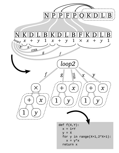
Figure 2: Representing local macros. A macro version and expanded version of a program invented for A1813 ($a(n)=(2n)!/n!$). Note that the macro here (K D L B) is not a proper program, only a sequence of actions.

Global Definitions

In this setup, we allow for arbitrarily many macros stored in a global array and shared across all programs. This makes the naming of the macros consistent in all programs, possibly making them easier to learn. Programs may refer to any macro stored in the global array, by writing its index in base 10. This again requires 10 additional actions (one for each digit) and a special action to separate the references to the macros. As in the local definition setup, the global macros may contain references to macros with lower indices. Figure 3 shows an example of the solution found for the sequence A14187https://oeis.org/A14187 - Cubes of palindromes. which involved three global macros that are altogether used five times in the body of the invented program.

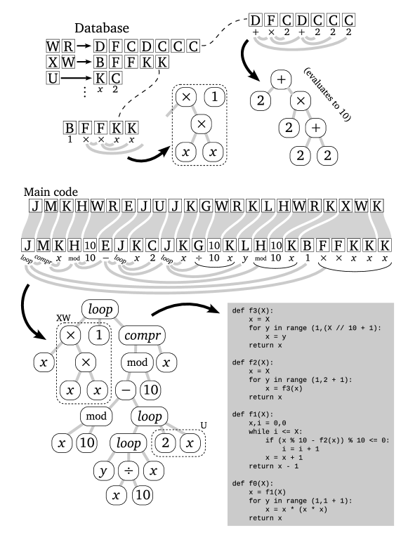
Figure 3: Representing global macros. A macro version and expanded version of a program invented for A14187 (cubes of palindromes). Note that two macros here (K C and B F F K K) are not proper programs, while the third one (D F C D C C C) is a program that evaluates to 10.

Introduction and use of local macros for a particular input integer sequence is completely a “local” decision of the trained NMT that generates the particular program. In the global case, we however need more coordination to introduce the global macros consistently. This can be done in various ways and we now use the following method. At every iteration of the overall loop, we add the ten most frequent sequences of actions to the array of global macros. To force the network to learn to use the global macros, we greedily (starting from the macros with the lowest indices) recognize sub-sequences of actions that correspond to the macros, and replace them with the macros’ names (indices) in the programs.

2.3 The Program Checker

In its most basic form the checker takes a program and a sequence and checks if that program generates the sequence. Since programs may depend on two variables, we say that the program $f(x,y)=p$ generates the finite sequence $(s_{x})_{0\leq x\leq n}$ if and only if

$$\forall x\in\mathbb{Z}.\ 0\leq x\leq n\Rightarrow f(x,0)=s_{x}$$

We say that a sequence $s$ has a solution if we have found a program $p$ generating it. The number of OEIS sequences with at least one solution is the number reported in all our experiments under the label solutions.

Timeout

The first issue when implementing a program checker is to determine the time limit for running the (generally non-terminating) programs. In particular, to adapt the time limit for longer sequences, we compute the generated terms in the order $f(0,0),f(1,0),f(2,0),...$ and stop the program if it has not generated the $n$-th term in less than $n\times t_{\mathit{call}}$ abstract time units. This effectively means that we give a timeout of $t_{\mathit{call}}$ time units per call with the time unused during previous calls added to the timeout of the current call.

This abstract time unit is computed to be an approximation of the number of CPU instructions needed to perform each operation. The cost of an operation is 1 for the $+,-,\times$ operations, it is 5 for the $\mathit{div},\mathit{mod}$ operations, and it is the number of bits of the result if the result is larger than 64 bits. Using the abstract time is also important to get accurate and repeatable measurements of the speed of the programs.

Hindsight Experience Replay

To augment the training data using a limited form of hindsight experience replay [1], we check our program against all OEIS sequences at the same time. This can be done effectively by organizing the sequences into a tree of sequences (Fig. 4) and stopping the checking as soon as the generated sequence reaches a leaf in that tree or takes a non-existing branch in the tree. All sequences (typically at most one) found along the path taken by the generated sequence are said to have a solution.

Figure 4: Tree of OEIS sequences with branches for primes (A40), even numbers (A5843) and Fibonacci numbers (A45).

Objectives

After each iteration we keep only the fastest and the smallest program (which could be the same) for each sequence $s$. The speed of a program for $s$ is the total number of abstract time units necessary to generate $s$. The size of a program is the number of operators/tokens in its linear representation. As soon as the checker has found a program that is a solution for a particular OEIS sequence, we compare it with the existing solutions for that sequence. We use the abstract time to select the fastest program among the ones that match the solutions. The fastest and smallest programs are also used as training examples for the next iteration of the loop.

2.4 Comprehension Limit

Evaluating each term of the sequence $\mathit{compr}(f,0),\mathit{compr}(f,1),\ldots,\mathit{compr}(f,n-1)$ separately is most of the time too slow. This computation can be sped up using the fact that each term can be computed from the preceding term in the sequence. In general, when executing a program containing comprehension operators, we precompute the results of applying $\mathit{compr}(f,i)$ for each $f$ appearing as the first argument of $\mathit{compr}$, where the number $i$ ranges from $0$ to $n_{\mathit{compr}}-1$. The number $n_{\mathit{compr}}$ is a parameter called the comprehension limit. The pre-computation times out if it takes more than $i\times t_{\mathit{call}}$ time units to produce the outputs for $\mathit{compr}(f,0),\ldots,\mathit{compr}(f,i)$. When the top program is executed, a call to a $\mathit{compr}(f,a)$ subprogram times out if no precomputed value exists for the input $i$ created by the subprogram $a$. Otherwise, the call returns the precomputed value for $\mathit{compr}(f,i)$ to the top program.

2.5 Choice of the Timeout Parameters

The two parameters that determine how long a program may be run for are the timer per call $t_{\mathit{call}}$ and the comprehension limit $n_{\mathit{compr}}$. A program times out if it exceeds the timeout or if one of the $\mathit{compr}$ expressions reaches the comprehension limit or if an integer with an absolute value larger than or equal to $2^{1025}$ is produced. We may run either a fast check, a slow check or a hybrid check on the set of candidate programs. The fast check uses as parameters $t_{\mathit{call}}=1000$, $n_{\mathit{compr}}=20$, and the slow check uses $t_{call}=100000$, $n_{\mathit{compr}}=200$.

Hybrid Check

The hybrid check tries to achieve the performance of the fast check while retaining most of the additional solutions found by the slow check. The first phase of the hybrid check is the fast check. After this check, we look at the programs that generated a prefix of an OEIS sequence but could not complete the full task. At this point, if we were to perform the slow check on all those prefix-generating programs, the hybrid check would take a time equivalent to the slow check. To get a gain in performance, we select only the ones that are the smallest for each prefix to be tested for a longer time. Fast programs implicitly differentiate themselves from others by generating longer prefixes, therefore are also selected by the same criteria for further checking.

In most of our experiments, we use the hybrid check because it is about 15 times faster than the slow check. However, since it does not test all programs with the long timeout, it misses out on some solutions found by the slow check. In the longer NMT runs, we eventually switched from the hybrid check to the more robust slow check, to discover more solutions.

3 OEIS Synthesis as an NMT Task

Neural networks have in the last decade become competitive in language modeling and machine translation tasks, leading to applications in many areas. In particular, recurrent neural networks (RNNs) with attention [5] and transformers [37] have been recently applied in mathematical and symbolic tasks such as rewriting [24], autoformalization [38] and synthesis of mathematical conjectures and proof steps. Many of these tasks are naturally formulated as sequence-to-sequence translation tasks.

NMT Representation

The OEIS program synthesis can also be cast as such a task. In this work we therefore experiment with replacing the TNN architecture with a reasonably fast encoder-decoder neural machine translation (NMT) system. In particular, we represent the input integer sequence as a series of digits, separated by an additional token at the integer boundaries. Since the initial integers in a sequence are typically smaller and may be more informative for the NMT decoding phase, we reverse the input sequences. The output program is also represented as a sequence of tokens in Polish notation (Fig. 5).

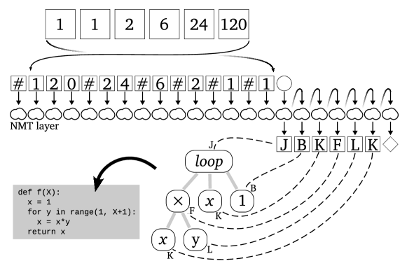
Figure 5: Representing sequences and solutions for NMT.

Beam Search

To make full use of the NMT capabilities, we also replace the original MCTS search with a wide beam search during the NMT decoding. Beam search with width $N$ is an alternative to greedy decoding. Instead of a single greedily best output, NMT in beam search keeps track of the $N$ conditionally most probable outputs, updating their ranking after each decoding step. When the NMT decoding for a particular input OEIS sequence $s$ is finished, the final $N$ best outputs can be used as NMT’s $N$ alternative suggestions of programs that solve $s$.

NMT Framework and Hyperparameters

After several initial evaluations we have chosen for the experiments Luong’s NMT framework [19]. It works efficiently on our hardware both in the training and wide-beam inference mode, and we were able to find suitable hyperparameters for it [38]. In more detail, we use for most experiments a 2-layer bidirectional LSTM equipped with the “scaled Luong” attention and 512 units. In our NMT experiments (Section 5) we start by using one NMT model for training and inference, using many default NMT hyperparameters. As the iterations progress, we gradually adjust the parameters and add more models trained differently and on differently selected data. We also experiment with larger models.

Combining NMT Models

In most NMT runs we train two to four different NMT models in parallel each on its own GPU. We then run the inference with two of them in parallel, thus using all 4 GPUs on the server. The rationale behind training and inference with differently trained models is the standard portfolio argument, used routinely, e.g., in automated theorem proving [31, 34, 27, 14, 13]. A complementary portfolio of specialists typically outperforms a single general strategy. In feedback loops that alternate between proof search and learning [36], this also further benefits the learning phase, since each learner can additionally use the training data accumulated by others. In Section 5 we see that this indeed considerably improves the performance.

Continuous training

NMT models can be trained either only on the latest version of the solutions or in a continuous way. The latter method re-uses the model trained in the previous iteration and trains it on the latest data for more steps. This makes such model more stable, being eventually trained for orders of magnitude more steps. It also makes it different from the models trained from scratch only on the latest data. Even when only a few solutions arrive in the latest iteration, the network is training further on the whole latest corpus, thus becoming smarter and hopefully more competent for the next inference phase. The models trained only on the latest corpus are on the other hand less concerned by the old (slower/longer) solutions and more focused on exploring the latest ones.

4 Experiments with a Tree Neural Network

In our previous work [10], a tree neural network (TNN) serves as a machine learning model. In the following, we test how varying a range of parameters influences the self-learning process. To test the limit of the TNN, we run the TNN-guided learning loop for 500 generations instead of the original 25. This last experiment of this section also provides a baseline for the NMT experiments.

Varying Parameters

We investigate the effect of three different parameters: the TNN embedding size, the choice of the programming language and the choice of the objectives. Unless specified otherwise, the default value for those parameters are respectively 96 for the dimension, the previously described programming language (see Section 2.2) and the selection of the smallest and fastest programs.

Table 1: Evolution of the number of solutions of runs with various parameters over the first 20 iterations

	Iteration	0	5	10	15	20
	16	2005	14920	19674	21163	22203
	32	1972	17608	23490	25750	27351
Embedding size	64	2017	18156	23737	26490	28463
	96	1993	16051	20127	22890	24718
	96 l.s.	3771	20434	25378	28361	30344
	minimal	1157	7096	8547	9126	9965
Language (embed. 64)	default	2017	18156	23737	26490	28463
	extra	1763	18690	23757	26905	28794
	both	3771	20434	25378	28361	30344
Objective (local search)	small	3725	20501	26231	29124	31520
	fast	3716	21021	26270	29326	31421

In Table 1, we present the results of running experiments with different parameters for 20 iterations. In a first experiment (first block in the table), we observe that the number of solutions increases with the dimension until dimension 64. Surprisingly, dimension 96 gave worse results, this is mainly due to the fact that larger networks are more expensive to compute and therefore produce fewer programs. As a countermeasure, we introduce a local search (l.s.) that tests all programs that are one action away from being constructed in the search tree. This balances the generation time and checking time better, leading to an increase in the number of solutions. In a second experiment (second block in the table), we measure how changing the programming language affects the performance. All the experiments presented in this block use dimension 64. The minimal row runs the self-learning loop with an even more minimalistic programming language consisting of four operators: $0,\mathit{successor},\mathit{predecessor},\mathit{loop}$. This makes the learning much more challenging. One of the reasons is that creating a large number such as one million in this language requires at least one million steps. Therefore, it is impossible to produce large numbers within the checker’s time limit. Such considerations justify the inclusion in the default language of operators efficiently computed by current hardware such as $+$ and $\times$. The extra row shows what happens when we include the extra constants 3,4,…,10 as primitive operators. This inclusion makes the computation of large numbers more efficient and increases the performance of our system slightly. However, adding more and more primitive operators introduces human bias that we would rather avoid. In a third experiment (third block in the table), the results of learning with different program objectives are presented. All these experiments were performed with dimension 96 and local search. The small (resp. fast) row shows the effect of only collecting and learning from the smallest (resp. the fastest) programs for a given OEIS sequence. The results imply that focusing on one objective at a time simplifies the work of the machine learner. Yet, we expect more synergy between the two objectives to occur during longer runs.

Long Run

The result of a long-lasting experiment, running for 500 iterations with the default parameters and local search, is shown in Fig. 6 (tnn). To fit also the NMT runs, we display only the first 190 iterations, however the average increments (Fig. 7, tnn) between iteration 200 and 300 drops below 20. At the end of the run, the TNN seems to have reached its limit and about five new solutions are found at each iteration. As we will see in Section 5, due to its larger embedding size and its more involved architecture and the introduction of continuous training, the main NMT experiment does not plateau and reaches a much higher number in an equivalent amount of time.

5 Experiments with NMT

5.1 Basic run ($\mathit{nmt}_{0}$)

In the basic NMT runhttps://github.com/Anon52MI4/oeis-alien/tree/master/run0 ($\mathit{nmt}_{0}$), we are running the loop in a way that is most similar to the TNN run. In particular, the checking phase is interleaved with training a single NMT $\mathit{model}_{0}$, which is then used for the search phase, implemented as NMT inference using a wide beam search. As in the TNN experiment, we start with the initial random iteration which yields 3771 solutions. Then we run 100 iterations of the NMT-based learn-generate-check loop.

Training

We use a batch size of 512 and SGD with a learning rate of 1.0. In each iteration, we train on the latest set of solutions, for 12000 steps. From iteration 45, we increased the number of training steps to 14000 to adjust for the growing number of training examples.This corresponds to 438 epochs in iteration 3 where there are about 14k examples, 92 epochs in iteration 44 (67k examples), 107 epochs in iteration 45 (after switching to 14000 steps), and 76 epochs in iteration 101 (81k examples). On one GPU (GTX1080 Ti, 12G RAM) the training takes on average 100m with 12000 steps and 130m with 14000 steps. The bleu scores on small test and development sets are typically between 25 and 30. There is only one memory crash (iteration 97).

Inference

We use two GPUs in parallel (splitting OEIS into two parts), each with a batch size of 32 and beam width 240. These values are determined experimentally, to load the GPUs efficiently without memory crashes. The parallelized inference time grows from 2 to 8 hours, increasing as the iterations invent longer examples, and the trained network and the beam search become less confident about when to stop decoding. Each inference phase yields $240\cdot 351663=84.4M$ program candidates that are then handed over to the checking phase.

Checking

We use the hybrid checking mode (Section 2.5) parallelized over 18 CPUs. The checking time grows from about 2 minutes to about 8-10 minutes. This is negligible compared to the NMT training and inference times. The 100 iterations of this loop took about a month of real time, reaching 46707 solutions (Fig. 6, nmt0). However, the increments drop below 200 (respectively 100) after iteration 37 (respectively 94).

5.2 Long extended run ($\mathit{nmt}_{1}$)

Since the time taken by one $\mathit{nmt}_{0}$ iteration reaches about half a day towards the end of the run, we explore more efficient approaches and further extensions and modifications. This leads to the longest runhttps://github.com/Anon52MI4/oeis-alien/tree/master/run1 $\mathit{nmt}_{1}$, which has at the time of submitting this paper reached 190 iterations and over 78000 solutions (Fig. 6, nmt1).The 190 $\mathit{nmt}_{1}$ iterations took 3 months on a 4-GPU server. Its remarkable property is that, unlike in $\mathit{nmt}_{0}$, the number of new solutions produced in each iteration rarely drops below 200, even after many iterations (Fig. 7, nmt1). This challenges the standard wisdom of “plateauing curves” appearing in the TNN and $\mathit{nmt}_{0}$ runs, and in many similar search-learn feedback loops [16, 23, 15].

Combining models

The $\mathit{nmt}_{1}$ run bootstraps from $\mathit{nmt}_{0}$, inheriting its first 20 iterations, thus starting with 34420 solutions. Then we start combining multiple NMT models (Section 3). Since iteration 21, we add training of $\mathit{model}_{1}$ to $\mathit{model}_{0}$. It is trained only on a randomly chosen half of the training set, however for twice as many steps/epochs. This yields a differently trained (and more focused) specialist in each iteration. The number of solution candidates produced by the inference phase thus doubles, to 168.8M. After de-duplication, this yields 32.5M unique candidates in iteration 21 compared to 13.4M in iteration 20. The checking (initially also using the hybrid mode) is still fast, taking 5 minutes on 18 CPUs. The difference to $\mathit{nmt}_{0}$ is remarkable: 687 new solutions in $\mathit{nmt}_{1}$ vs 272 in $\mathit{nmt}_{0}$ in iteration 21. This effect continues over the next iterations, see Fig. 7.

Further modifications

Since iteration 70, we start training $\mathit{model}_{1}$ in a continuous way (Section 3). By iteration 190 $\mathit{model}_{1}$ is thus trained for over 1.4M steps on the evolving data, making it quite different from other models. As we invent longer programs, we also allow training on longer sequences, raising the default NMT values of 50 input and 50 output tokens gradually to 80 and 140, respectively. Since iteration 156 we also add training of $\mathit{model}_{2}$, which takes specialization even further. It is trained for four times as many steps as $\mathit{model}_{0}$ on a random quarter of the data. The bleu scores of $\mathit{model}_{0}$ are at this point low, due to the larger size of the data, while $\mathit{model}_{2}$ still achieves scores above 25. We then use $\mathit{model}_{0}$ only as a backup when $\mathit{model}_{2}$ diverges. Since iteration 159 we switch from the hybrid check to the slow (full) check (Section 2.5), raising the checking time from 45m (iteration 158) to 6h, and the number of solutions from 178 to 860 (Fig. 7, nmt1). This jump is likely due to many programs using comprehension being newly allowed. It includes sudden solutions for hundreds of problems that combine congruence operations and primes.https://bit.ly/3QPkquE

Bigger Network

Since iteration 170, we add continuous training of a bigger $\mathit{model}_{3}$ which uses 1024 units instead of 512. To keep all models and phases in sync, we train $\mathit{model}_{3}$ for fewer steps (8000), decreasing also its batch size and inference width to 288 and 120, respectively. Table 2 analyzes the benefits of using $\mathit{model}_{3}$, $\mathit{model}_{2}$ and $\mathit{model}_{0}$ in addition to $\mathit{model}_{1}$over 12 iterations (175-186).

Table 2: Influence of using models M3, M2 or M0 for inference in addition to M1. UC are unique candidates (millions), NS new solutions added, TS total solutions including all found so far, and OS own solutions, i.e., the sequences covered by the current iteration.

Iteration	175	176	177	178	179	180
Model	M2	M3	M0	M2	M2	M2
UC	101.7	79.7	64.7	99.7	96.0	106.2
OS	74746	74916	74130	75196	75386	75313
TS	75471	75666	75795	75985	76160	76404
NS	260	195	129	190	175	244
Iteration	181	182	183	184	185	186
Model	M2	M2	M2	M2	M3	M3
UC	105.8	106.1	106.7	101.1	84.5	85.7
OS	75686	75986	76271	76397	76793	77007
TS	76656	76861	77055	77244	77411	77577
NS	252	205	194	189	167	166

The number of unique candidates is much lower for $\mathit{model}_{3}$ (due to the beam width) than for $\mathit{model}_{2}$, however still higher than for $\mathit{model}_{0}$, which is at this point likely undertrained. In general, $\mathit{model}_{3}$ performs better than $\mathit{model}_{0}$, but is inferior to $\mathit{model}_{2}$. A faster model, producing twice as many plausible candidates in the same amount of time, is here better than a slower model which is a bit more precise.Also, $\mathit{model}_{3}$ is trained continuously and may resemble more $\mathit{model}_{1}$, providing fewer different candidates. And $\mathit{model}_{2}$ is trained only on a random quarter of the latest data, making it even more orthogonal to the continuous models that have seen much more data.

5.3 Runs with Local and Global Macros

As the average program size grows in $\mathit{nmt}_{1}$ (Fig. 8), the NMT decoding times increase, taking almost 12h in the latest iterations. Verbatim repetition of blocks of code also feels suboptimal to human programmers. This motivates later additional runs $\mathit{nmt}_{2}$ and $\mathit{nmt}_{3}$, where we experiment with using local and global macros. Apart from allowing these additional macro mechanisms (Section 2.2), the two runs resemble run $\mathit{nmt}_{1}$. In each of them we train the basic $\mathit{model}_{0}$ together with the continuous $\mathit{model}_{1}$, and infer with both of them. Since the sequences are shorter (making $\mathit{model}_{0}$ easier to train), we have not so far experimented with $\mathit{model}_{2}$ here. While the two runs seem superior to $\mathit{nmt}_{1}$ in Fig. 7, this is mainly due to the use of both models since iteration 2 (instead of iteration 21 in $\mathit{nmt}_{1}$), and also an earlier switch to the slow check (iteration 75 in $\mathit{nmt}_{2}$ and iteration 67 in $\mathit{nmt}_{3}$). The two runs also do not significantly complement $\mathit{nmt}_{1}$: each of them adds less than 2800 solutions to $\mathit{nmt}_{1}$. This may mean that the alien system $\mathit{nmt}_{1}$ has so far less trouble than humans with expanding everything and the use of definitions is not as critical as in humans. None of the two runs has however reached iteration 100 yet, making the comparison with $\mathit{nmt}_{1}$ only preliminary. Especially the statistics of the use of global macroshttps://bit.ly/3ZNe7fm in $\mathit{nmt}_{3}$ are interesting, and can be used for analyzing the evolution of its coding trends.

Figure 6: Number $y$ of solutions after $x$ iterations

Figure 7: Number of new solutions $y$ found at each iteration $x$.

Figure 8: Average size of the smallest (respectively fastest) programs discovered within $x$ iterations

Figure 9: Average speed of the fastest (respectively smallest) programs discovered within $x$ iterations

Figure 10: Evolution of the average size $y$ of smallest programs for 100 additional iterations starting from the iteration they were first discovered

Figure 11: Evolution of the average size $y$ of fastest programs for 100 additional iterations starting from the iteration they were first discovered

6 Analysis of the Results

We provide a statistical analysis of the 78118 solutions found during the $\mathit{nmt}_{1}$ run and discuss the details of some techniques developed by our system. More information on the $\mathit{nmt}$ runs is available in our anonymous repository.https://bit.ly/3iVIfnX For some sequences, its subdirectoryhttps://bit.ly/3XHZsjK contains our analysis of the evolutionhttps://bit.ly/3iJ4oGdhttps://bit.ly/3HfwemI and proliferationhttps://bit.ly/3ZNExO4https://bit.ly/3IVzrJz of important programs such as primes and sigma, as well as proofs that some of the alien programs match the human OEIS intention.https://bit.ly/3QPB25ohttps://bit.ly/3WlVHPMhttps://bit.ly/3XJi96j See also the appendix for more details. Noteworthy sequences from this repository include convolution of primes with themselves,https://bit.ly/3XJi96j showing the proficiency of our system with primes. Motzkin numbershttps://bit.ly/3QPB25o [39] are an example where our synthesized programs rely on a pairing function. This programming technique, re-invented by our system, packs two variables into one, allowing further programs (see Appendix B for details). A solution for the unique monotonic sequence of nonnegative integers satisfying $a(a(n))=3n$ is needed in solving a problem in $27^{th}$ British Mathematical Olympiad.https://bit.ly/3wjmqSg

Evolution of the Programs

Fig. 8 shows the evolution of the average size and Fig. 9 the speed of the solutions. We see that as new solutions are found, they become longer and typically also take more time. However, there are interesting exceptions to the latter rule (Fig. 9), as more efficient code is invented and propagated by the alien system. We thus also measure the gradual size reduction (Fig. 10) and time reduction (Fig. 11) for the short and fast solutions (respectively). This is for each sequence computed for 100 iterations after its first solution was found. We see that the iterations induce a remarkable speedup of the invented fast solutions (Fig. 11).

Generalization of the Solutions to Larger Indices

OEIS provides additional terms for some of the OEIS entries in b-files. Among the 78118 solutions, 40,577 of them have a b-file that contains 100 additional terms for their OEIS entry. We evaluate both the small and the fast programs with the slow check parameters on the 100 additional terms. Here, 14,701 small and 11,056 fast programs time out. Among the programs that do not time out, the percentage of generalizing programs (producing matching additional terms) is 90.57% for the slow programs and 77.51% for the fast programs. A common error is reliance on an approximation for a real number, such as $\pi$.

7 Related work

The closest related recent work is [8], done in parallel to our project. The goal there is similar to ours but their general approach is focused on training a single model using supervised learning techniques on synthetic data. In contrast, our approach is based on reinforcement learning: we start from scratch and keep training new models as we discover new OEIS solutions. The programs generated in [8] are recurrence relations defined by analytical formulas. Our language seems to be more expressive. For example, our language can use the functions it defines by recurrence using $\mathit{loop}$ and $\mathit{loop2}$ as subprograms and construct nested loops. The performance of the model in  [8] is investigated on real number sequences, whereas our work focuses only on integer sequences. Overall, it is hard to directly compare the performance of the two systems. Our result is the number of OEIS sequences found by targeting the whole encyclopedia, whereas [8] reports the test accuracy only on 10,000 easy OEIS sequences. A related recent small-scale experiment is reported in [4], where a model pre-trained on many code repositories is used (i.e., the system is not developed from scratch as we investigate here), using a language and feedback-loop setting similar to the one introduced by us in [10]. The reported result there is 11.5% of 10000 easy OEIS sequences. This is also incomparable to our system, where the main point is to measure the capability of the system to develop new ideas on its own (i.e., without the potential contamination with ideas seen in the pre-training), and the system runs on the whole OEIS, reporting orders of magnitude higher numbers of solutions.

The deep reinforcement learning system DreamCoder [9] has demonstrated self-improvement from scratch in several programming tasks. Its main contribution is the use of definitions that compress existing solutions and facilitate building new solutions on top of the existing ones. Our experiments with local and global macros are however so far inconclusive. While humans certainly benefit from introducing new names, concepts and shortcuts, it is so far unclear if it results in a clear improvement in our current setting. Another related system is developed within the LODA [17] project, where the methods, experiments and resources are however yet to be fully described. Within the theorem proving community, the development of methods for term synthesis has been explored in inductive theorem proving [6] and in counterexample generators [2, 3].

While the previous version of our system used MCTS inspired by AlphaGoZero [28], the current NMT approach uses just straightforward beam search. The general search-verify-learn positive feedback loop between ML-guided symbolic search and statistical learning from the verified results has been used for a long time in large-theory automated theorem proving, going back at least to the MaLARea system [33, 36]. Its recent instances include systems such as rlCoP [16] and ENIGMA [15]. Such systems can be also seen as synthesis frameworks, where the mathematical object synthesized by the guided search is however the full proof of a theorem, rather than just a particular interesting witness or a conjecture. Synthesis of full proofs of mathematical theorems is an all-encompassing task that can be extremely hard in cases like Fermat’s Last Theorem. Our current setting may thus also be seen as an attempt to decompose this all-encompassing task into smaller interesting subtasks that can be analyzed separately.

8 Conclusion

As of January 25, 2023, all of the runs have together invented from scratch solutions for 84587 OEIS sequences. This is more than three times the number (27987) invented in our first experiments [10]. This is due to several improvements. We have started to collect both the small and fast solutions and learn jointly from them. We have seen that this gradually leads to a large speedup of the fast programs, as the population of programs evolves. This likely allows invention of further solutions that are within our time limit, thanks to the discovery of the faster and faster components. The improvements (learning) on the symbolic side thus likely complement and co-evolve with the statistical learning used for guiding the synthesis. We have also started to use relatively fast neural translation models, their specialization on random subsets, their combinations and continuous training, and a wide beam search instead of MCTS. The experiments suggest that these techniques are useful, leading to a high rate of program invention even after the 190 iterations in the longest NMT run. This is encouraging since many of the solved OEIS problems seem nontrivial. The trained system could thus be used as a search tool assisting mathematicians. There is also a wealth of related mathematical tasks that can be cast in a similar synthesis setting, and combined with other tools, such as automated theorem provers.

A crucial element of our setting is the fact that NMT is used to produce an interpretable symbolic representation. It would be practically unusable if we relied purely on neural approximation of arbitrary functions and the task for NMT was to directly produce the next 100 numbers in each OEIS sequence. The interpretable symbolic representation is critical for the generalization capability of the overall system and its capability to learn from itself. The overall alien system can also be seen as an example of a very weakly supervised evolutionary architecture where simple high-level principles (Occam’s razor and efficiency) govern the development and training of the lower-level statistical component (NMT). Rather than one-time training on everything that has been already invented by humans so far, as done by today’s large language models, the system here starts from zero knowledge and progresses towards increasingly nontrivial knowledge and skills. Such feedback loops thus seem to be a good playground for exploring how increasingly intelligent systems emerge. Note that thanks to the Turing completeness of the language, this particular playground is (unlike games like Chess and Go) not limited in its expressivity, and can in principle lead to the development of arbitrary complex algorithms.

9 Acknowledgments

We thank Chad Brown, David Cerna, Hugo Cisneros, Tom Hales, Barbora Hudcova, Jan Hula, Mikolas Janota, Tomas Mikolov, Jelle Piepenbrock, and Martin Suda for discussions, comments and suggestions. This work was partially supported by the CTU Global Postdoc funding scheme (TG), Czech Science Foundation project 20-06390Y (TG), ERC-CZ project POSTMAN no. LL1902 (TG), Amazon Research Awards (TG, JU), EU ICT-48 2020 project TAILOR no. 952215 (JU), and the European Regional Development Fund under the Czech project AI&Reasoning with identifier CZ.02.1.01/0.0/0.0/15_003/0000466 (MO, JU).

Appendix A Resources Used by the Experiment

The average GPU power consumption during inference is 800W: 200W per each of the four GTX 1080 Ti cards used for inference. The average GPU power consumption during training is 350W: 175W per each of the two GTX 1080 Ti cards used for the two kinds of training done in most of the iterations.

The training takes approximately 3 hours and the inference 10.5 hours (iteration 140 of the longest run). This means that the average GPU consumption per hour is $(3*350+10.5*800)/13.5=700W$. Additionally, we estimate the non-GPU (CPUs, disks, etc.) consumption to be on average 150W per hour (the server’s CPUs are mostly idle). It took about three months to do the 190 iterations of the longest run. This is $90*24=2160$ hours. The estimated power consumption for the 190 iterations is thus $2160*(700+150)=1836$ kWh. Assuming a cost in the range of 150-250 EUR per MWh, the main experiment’s electricity cost is between 270 and 460 EUR. The three shorter experiments have so far run for about half as many iterations and are also using on average less resources (fewer GPUs, shorter inference length). The estimated power consumption for all experiments is thus likely below 4 MWh, and the total electricity cost below 1000 EUR.

Appendix B Triangle Coding

Our system has found a correspondence between a pair of non-negative integers $(x_{a},x_{b})$ where $x_{a}\geq x_{b}$, and a single non-negative integer $x$ by enumerating the following sequence of pairs $(x_{a},x_{b})$ with non-negative integers:

$$(0,0),(1,0),(1,1),(2,0),(2,1),(2,2),(3,0),\ldots.$$

In one direction, it computes $x=\frac{x_{a}\times(x_{a}+1)}{2}+x_{b}$ in order to “encode” the pair $(x_{a},x_{b})$. Decoding of a single non-negative integer $x$ can be calculated as $(x_{a},x_{b})=(f_{0}(x)-f_{1}(x),f_{0}(x))$, where the functions $f_{0},f_{1}$ can be implemented in Python for example as follows (an actual code invented by the program generator). Note that the function $f_{0}$ computes $x_{b}$, and the function $f_{1}$ computes $x_{b}-x_{a}$ (a non-positive integer).

⬇

def f0(X):

x = X

for y in range (1,(2 + (X // (1 + (2 + 2)))) + 1):

x = x - (y if (y - x) <= 0 else 0)

return x

def f1(X):

x = X

for y in range (1,(2 + (X // (1 + (2 + 2)))) + 1):

x = x - (0 if x <= 0 else (1 + y))

return x

This representation was initially discovered when our system found solutions for the sequences A2262,https://oeis.org/A002262 and A25581.https://oeis.org/A025581 Indeed, $f_{0}$ is a solution for A2262 invented in the first iteration and $-f_{1}$ is a solution for A25581 invented during the $9^{th}$ iteration.

B.1 Number of steps

In order to calculate $f_{0}$ and $f_{1}$, one must perform approximately $\sqrt{2x+\frac{1}{4}}-\frac{1}{2}$ steps in a subtracting loop. Since the programming language is based on for loops, the programs are approximating the number of subtracting steps with a function that can be easily obtained using the basic arithmetical operations. In particular, the code above uses approximations with $2+x/5$ where 5 is written as $1+(2+2)$ (our basic language only supports constants 0,1,2). The program generator has experimented with many (over 80) such bounds, the vast majority of such bounds are of the shape $a+x/b$ or $a+2(x/b)$ where $a$, $b$ are constants. As the speed of computing with larger numbers becomes more important, the slope of the approximation flattens, with $b$ reaching values over $50$. We have collected all such subprograms used in the generated programs, and plotted the bounds in Figure 12 and Figure 13. The approximated function $\sqrt{2x+\frac{1}{4}}-\frac{1}{2}$ is plotted with a black dashed line. All the found valid bounds are plotted in green, all the invalid bound attempts are plotted in red.

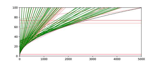
Figure 12: Linear bounds (in red or green) for $y=\sqrt{2x+\frac{1}{4}}-\frac{1}{2}$ (in black) invented by the system with $x\leq 5000$.

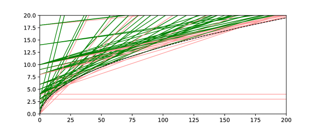
Figure 13: Linear bounds (in red or green) for $y=\sqrt{2x+\frac{1}{4}}-\frac{1}{2}$ (in black) invented by the system with $x\leq 200$.

B.2 Triangle coding in action

The triangle coding turned out to be useful in many cases. The designed language for our programs only supports a maximum of two variables but using the triangle coding, a pair of variables can be temporarily packed into one. A simple example is sequence A279364https://oeis.org/A279364 – sum of 5th powers of proper divisors of n. A human programmer could implement this sequence as:

⬇

def f(X):

res = 0

for y in range(1,X+1):

res = res + (y**5 if (X+1) %

return res

There are three variables used in the body of the loop, in particular res, y, and X. Since the native language supports only two variables available at every moment, this Python code cannot be straightforwardly translated into the language of our programs. Nevertheless, the program generator has found a workaround using the triangle coding – it packs X and y into a single natural number, so it can perform the summing loop adding to res, and in order to decode what to add to res, it unpacks the pair, and checks whether y divides X+1.

The code generated by NMT for A279364

is as follows:

A279364 Sum of 5th powers of proper divisors of n.
371326 59293 555688 1 870552 1 1082401 161295 1419890 19933 2206525 1
2476132 371537 3336950 1 4646784 1 5315740 821793 6436376 1 9301876
16808 9868783

size 94, time 1335684: loop2 ((loop (loop2 ((loop ((((x * x) * x) * x)
* x) 1 (1 + y)) * (if (x mod (1 + y)) <= 0 then 1 else 0)) 0 1 (1 -
(loop (x - (if x <= 0 then 0 else y)) (1 + (2 + (2 + (x div (1 + (2 *
(2 + 2))))))) (1 + x))) (loop (x - (if (y - x) <= 0 then y else 0)) (2
+ (2 + (x div (1 + (2 * (2 + 2)))))) x)) 1 y) + x) (1 + y) x 0 (((x *
x) - x) div 2)

K K F K F K F K F B B L D J K B L D H B A I F A B B K K A L I E B C C
K B C C C D F D G D D D B K D J E K L K E L A I E C C K B C C C D F D
G D D K J N B L J K D B L D K A K K F K E C G N

⬇

def f3(X,Y):

x = 1 + Y

for y in range (1,1 + 1):

x = (((x * x) * x) * x) * x

return x

def f4(X):

x = 1 + X

for y in range (1,(1 + (2 + (2 + (X // 9)))) + 1):

x = x - (0 if x <= 0 else y)

return x

def f5(X):

x = X

for y in range (1,(2 + (2 + (X // 9))) + 1):

x = x - (y if (y - x) <= 0 else 0)

return x

def f2(X):

x,y = 1 - f4(X), f5(X)

for z in range (1,1 + 1):

x,y = (f3(x,y) * (1 if (x %

return x

def f1(X,Y):

x = Y

for y in range (1,1 + 1):

x = f2(x)

return x

def f0(X):

x,y = 0, ((X * X) - X) // 2

for z in range (1,X + 1):

x,y = (f1(x,y) + x), (1 + y)

return x

for x in range(32):

print (f0(x))

The number $9$ in these functions is used as a shorthand for $1+2*(2+2)$. Functions f4, f5 are calculating the triangle coding, f3 is the fifth power, f1 is just a dummy function using Y instead of X for f2. Finally, f2 is returning either $(b+1)^{5}$, or 0 depending on whether $b+1$ divides $a+2$ or not where $(a,b)$ if the triangle coding pair of X, and f0 is summing over all the pairs $(a,b)$ going from (X-1,0) to (X-1,X-1).

Appendix C Evolution and Proliferation

We analyze the evolution of the solutions found for the OEIS sequence of prime numbers.The tables shown here for primes are also in our repository https://bit.ly/3XHZsjK, together with similar tables for the sigma function (sum of the divisors). The exact iterations of their discovery are shown in our repository, together with their size and speed.https://bit.ly/3iJ4oGd The 24 invented programs are shown in Table 3.

Table 3: The 24 programs for primes.

Nr	Program
P1	(if x <= 0 then 2 else 1) + (compr (((loop (x + x) (x mod 2) (loop (x * x) 1 (loop (x + x) (x div 2) 1))) + x) mod (1 + x)) x)
P2	1 + (compr ((((loop (x * x) 1 (loop (x + x) (x div 2) 1)) + x) * x) mod (1 + x)) (1 + x))
P3	1 + (compr (((loop (x * x) 1 (loop (x + x) (x div 2) 1)) + x) mod (1 + x)) (1 + x))
P4	2 + (compr ((loop2 (1 + (if (x mod (1 + y)) <= 0 then 0 else x)) (y - 1) x 1 x) mod (1 + x)) x)
P5	1 + (compr ((loop (if (x mod (1 + y)) <= 0 then (1 + y) else x) x (1 + x)) mod (1 + x)) (1 + x))
P6	1 + (compr ((loop (if (x mod (1 + y)) <= 0 then (1 + y) else x) (2 + (x div (2 + (2 + 2)))) (1 + x)) mod (1 + x)) (1 + x))
P7	compr ((1 + (loop (if (x mod (1 + y)) <= 0 then (1 + y) else x) x x)) mod (1 + x)) (2 + x)
P8	1 + (compr ((loop (if (x mod (1 + y)) <= 0 then (1 + y) else x) (1 + ((2 + x) div (2 + (2 + 2)))) (1 + x)) mod (1 + x)) (1 + x))
P9	compr (x - (loop (if (x mod (1 + y)) <= 0 then (1 + y) else x) x x)) (2 + x)
P10	compr (x - (loop (if (x mod (1 + y)) <= 0 then 2 else x) (x div 2) x)) (2 + x)
P11	1 + (compr ((loop (if (x mod (1 + y)) <= 0 then (1 + y) else x) (1 + (x div (2 + (2 + 2)))) (1 + x)) mod (1 + x)) (1 + x))
P12	compr ((x - (loop (if (x mod (1 + y)) <= 0 then y else x) x x)) - 2) (2 + x)
P13	1 + (compr ((loop (if (x mod (1 + y)) <= 0 then (1 + y) else x) (2 + (x div (2 * (2 + (2 + 2))))) (1 + x)) mod (1 + x)) (1 + x))
P14	compr ((x - (loop (if (x mod (1 + y)) <= 0 then y else x) x x)) - 1) (2 + x)
P15	1 + (compr (x - (loop (if (x mod (1 + y)) <= 0 then (1 + y) else x) (2 + (x div (2 * (2 + (2 + 2))))) (1 + x))) (1 + x))
P16	compr (2 - (loop (if (x mod (1 + y)) <= 0 then 0 else x) (x - 2) x)) x
P17	1 + (compr (x - (loop (if (x mod (1 + y)) <= 0 then 2 else x) (2 + (x div (2 * (2 + (2 + 2))))) (1 + x))) (1 + x))
P18	1 + (compr (x - (loop (if (x mod (1 + y)) <= 0 then 2 else x) (1 + (2 + (x div (2 * (2 * (2 + 2)))))) (1 + x))) (1 + x))
P19	1 + (compr (x - (loop2 (loop (if (x mod (1 + y)) <= 0 then 2 else x) (2 + (y div (2 * (2 + (2 + 2))))) (1 + y)) 0 (1 - (x mod 2)) 1 x)) (1 + x))
P20	1 + (compr (x - (loop2 (loop (if (x mod (1 + y)) <= 0 then 2 else x) (1 + (2 + (y div (2 * (2 * (2 + 2)))))) (1 + y)) 0 (1 - (x mod 2)) 1 x)) (1 + x))
P21	1 + (compr (x - (loop2 (loop (if (x mod (2 + y)) <= 0 then 2 else x) (2 + (y div (2 * ((2 + 2) + (2 + 2))))) (1 + y)) 0 (1 - (x mod 2)) 1 x)) (1 + x))
P22	1 + (compr (x - (loop2 (loop (if (x mod (2 + y)) <= 0 then 2 else x) (2 + (y div (2 * (2 * (2 + 2))))) (1 + y)) 0 (1 - (x mod 2)) 1 x)) (1 + x))
P23	2 + (compr (loop (x - (if (x mod (1 + y)) <= 0 then 0 else 1)) x x) x)
P24	loop (1 + x) (1 - x) (1 + (2 * (compr (x - (loop (if (x mod (2 + y)) <= 0 then 1 else x) (2 + (x div (2 * (2 + 2)))) (1 + (x + x)))) x)))

We can observe how these 24 programs propagate through the population of all programs, as they evolve in the iterations. This is shown in Table 4 and Table 5. We can see that, e.g., P5 (size 25, time 515990), gets quickly replaced by P6 (size 33, time 98390) and P7 (size 23, time 519654) after their invention. P6 is more than five times faster than P5, while P7 is smaller. Therefore they are included in the training data instead of P5 when they are invented. While there are still other programs in the training data using P5 as a subprogram, their faster/smaller versions get eventually also reinvented as the newly trained NMT increasingly prefers to synthesize programs that contain P6 or P7. This illustrates the dynamics of the overall alien system. The training of the neural synthesis component (NMT) evolves, governed by more high-level evolutionary fitness criteria, which are in our case size (Occam’s razor) and speed (efficiency).

Table 4: Proliferation of the 24 programs for primes.

Iter	P1	P2	P3	P4	P5	P6	P7	P8	P9	P10	P11	P12	P13	P14	P15	P16	P17	P18	P19	P20	P21	P22	P23	P24
25	0	0	0	0	0	0	0	0	0	0	0	0	0	0	0	0	0	0	0	0	0	0	0	0
26	6	0	0	0	0	0	0	0	0	0	0	0	0	0	0	0	0	0	0	0	0	0	0	0
27	7	0	0	0	0	0	0	0	0	0	0	0	0	0	0	0	0	0	0	0	0	0	0	0
28	8	0	0	0	0	0	0	0	0	0	0	0	0	0	0	0	0	0	0	0	0	0	0	0
29	9	0	0	0	0	0	0	0	0	0	0	0	0	0	0	0	0	0	0	0	0	0	0	0
30	10	0	0	0	0	0	0	0	0	0	0	0	0	0	0	0	0	0	0	0	0	0	0	0
31	4	6	0	0	0	0	0	0	0	0	0	0	0	0	0	0	0	0	0	0	0	0	0	0
32	6	6	0	0	0	0	0	0	0	0	0	0	0	0	0	0	0	0	0	0	0	0	0	0
33	8	1	6	6	0	0	0	0	0	0	0	0	0	0	0	0	0	0	0	0	0	0	0	0
34	12	4	6	6	1	0	0	0	0	0	0	0	0	0	0	0	0	0	0	0	0	0	0	0
35	7	12	6	0	9	0	0	0	0	0	0	0	0	0	0	0	0	0	0	0	0	0	0	0
36	4	10	6	0	17	0	0	0	0	0	0	0	0	0	0	0	0	0	0	0	0	0	0	0
37	3	4	6	0	18	6	1	0	0	0	0	0	0	0	0	0	0	0	0	0	0	0	0	0
38	2	3	1	0	12	18	11	0	0	0	0	0	0	0	0	0	0	0	0	0	0	0	0	0
39	2	3	1	0	9	56	31	0	0	0	0	0	0	0	0	0	0	0	0	0	0	0	0	0
40	2	5	2	0	7	59	49	9	1	0	2	0	1	0	0	0	0	0	0	0	0	0	0	0
41	1	2	3	0	4	52	58	42	23	0	13	0	8	0	0	0	0	0	0	0	0	0	0	0
42	0	2	4	0	3	44	50	38	60	8	11	0	55	0	0	0	0	0	0	0	0	0	0	0
43	0	2	12	0	0	37	55	14	116	35	16	7	90	0	0	0	0	0	0	0	0	0	0	0
44	0	2	13	0	0	28	40	6	176	73	19	8	122	9	12	0	0	0	0	0	0	0	0	0
45	0	2	9	0	0	19	24	4	147	185	26	16	94	25	29	0	7	0	0	0	0	0	0	0
46	0	2	4	0	0	11	14	0	101	256	21	14	66	64	30	0	29	0	0	0	0	0	0	0
47	0	0	0	0	0	9	4	0	55	290	23	3	43	116	16	6	62	14	0	0	0	0	0	0
48	0	0	0	0	0	8	0	0	22	261	16	0	34	192	10	6	89	30	0	0	0	0	0	0
49	0	0	0	0	0	8	0	0	6	195	11	0	36	225	8	6	99	34	0	0	0	0	0	0
50	0	0	0	0	0	5	0	0	2	154	8	0	29	168	6	6	108	39	0	0	0	0	0	0
51	0	0	0	0	0	4	0	0	0	121	7	0	21	97	6	6	113	43	0	0	0	0	0	0
52	0	0	0	0	0	2	0	0	0	118	8	0	12	62	6	6	110	51	0	0	0	0	0	0
53	0	0	0	0	0	1	0	0	0	59	7	0	15	33	6	6	125	62	0	0	0	0	0	0
54	0	0	0	0	0	1	0	0	0	41	4	0	16	17	6	9	137	72	0	0	0	0	0	0
55	0	0	0	0	0	2	0	0	0	32	4	0	15	9	6	17	147	82	0	0	0	0	0	0
56	0	0	0	0	0	1	0	0	0	29	4	0	10	7	6	39	152	98	0	0	0	0	0	0
57	0	0	0	0	0	1	0	0	1	28	3	0	9	5	6	103	142	108	0	0	0	0	0	0
58	0	0	0	0	0	0	0	0	1	17	3	0	7	4	6	146	146	120	0	0	0	0	0	0
59	0	0	0	0	0	0	0	0	1	11	3	0	6	2	0	179	153	122	0	0	0	0	0	0
60	0	0	0	0	0	0	0	0	1	6	3	0	3	2	0	206	148	121	0	0	0	0	0	0
61	0	0	0	0	0	0	0	0	0	6	3	0	3	1	0	220	139	138	0	0	0	0	0	0
62	0	0	0	0	0	0	0	0	0	5	3	0	2	0	0	245	118	145	0	0	0	0	0	0
63	0	0	0	0	0	0	0	0	0	5	3	0	2	0	0	263	103	160	0	0	0	0	0	0
64	0	0	3	0	0	0	0	0	0	6	4	0	2	0	0	284	87	162	0	0	0	0	0	0
65	0	0	13	0	0	0	0	0	0	5	4	0	1	0	0	303	74	173	0	0	0	0	0	0
66	0	0	34	0	0	0	0	0	0	3	2	0	1	0	0	315	67	174	0	0	0	0	0	0
67	0	0	53	0	0	0	0	0	0	1	1	0	1	0	0	321	64	180	0	0	0	0	0	0
68	0	0	61	0	0	0	0	0	0	1	1	0	1	0	0	323	66	178	0	0	0	0	0	0
69	0	0	67	0	0	0	0	0	0	1	1	0	1	0	0	325	63	178	0	0	0	0	0	0
70	0	0	70	0	0	0	0	0	0	1	1	0	1	0	0	324	60	182	0	0	0	0	0	0
71	0	0	72	0	0	0	0	0	0	1	1	0	1	0	0	330	56	181	0	0	0	0	0	0
72	0	0	73	0	0	0	0	0	0	0	2	0	1	0	0	332	57	190	0	0	0	0	0	0
73	0	0	72	0	0	0	0	0	0	0	2	0	1	0	0	330	58	191	0	0	0	0	0	0
74	0	0	71	0	0	0	0	0	0	0	3	0	1	0	0	336	56	189	0	0	0	0	0	0
75	0	0	74	0	0	0	0	0	0	0	2	0	1	0	0	340	55	192	0	0	0	0	0	0
76	0	0	77	0	0	0	0	0	0	0	1	0	0	0	0	341	57	195	0	0	0	0	0	0
77	0	0	79	0	0	0	0	0	0	0	1	0	0	0	0	343	56	191	0	0	0	0	0	0
78	0	0	79	0	0	0	0	0	0	0	1	0	0	0	0	344	57	201	0	0	0	0	0	0
79	0	0	81	0	0	0	0	0	0	0	0	0	0	0	0	344	56	200	0	0	0	0	0	0
80	0	0	80	0	0	0	0	0	0	0	0	0	0	0	0	346	55	210	0	0	0	0	0	0
81	0	0	75	0	0	0	0	0	0	0	0	0	0	0	0	351	55	206	0	0	0	0	0	0
82	0	0	77	0	0	0	0	0	0	0	0	0	0	0	0	354	53	206	0	0	0	0	0	0
83	0	0	77	0	0	0	0	0	0	1	0	0	0	0	0	360	53	207	0	0	0	0	0	0
84	0	0	76	0	0	0	0	0	0	1	0	0	0	0	0	360	53	208	0	0	0	0	0	0
85	0	0	74	0	0	0	0	0	0	1	0	0	0	0	0	363	53	207	0	0	0	0	0	0
86	0	0	75	0	0	0	0	0	0	0	0	0	0	0	0	361	54	205	0	0	0	0	0	0
87	0	0	77	0	0	0	0	0	0	0	0	0	0	0	0	359	54	198	0	0	0	0	0	0
88	0	0	80	0	0	0	0	0	0	1	0	0	0	0	0	359	54	199	0	0	0	0	0	0
89	0	0	83	0	0	0	0	0	0	1	0	0	0	0	0	357	56	196	0	0	0	0	0	0

Table 5: Proliferation of the 24 programs for primes.

Iter	P1	P2	P3	P4	P5	P6	P7	P8	P9	P10	P11	P12	P13	P14	P15	P16	P17	P18	P19	P20	P21	P22	P23	P24
90	0	0	82	0	0	0	0	0	0	1	0	0	0	0	0	345	56	194	0	0	0	0	0	0
91	0	0	81	0	0	0	0	0	0	1	0	0	0	0	0	331	50	188	0	0	0	0	0	0
92	0	0	66	0	0	0	0	0	0	0	0	0	0	0	0	322	31	176	9	1	0	0	0	0
93	0	0	56	0	0	0	0	0	0	0	0	0	0	0	0	313	18	162	37	17	0	0	0	0
94	0	0	41	0	0	0	0	0	0	0	0	0	0	0	0	303	9	145	52	30	0	0	0	0
95	0	0	26	0	0	0	0	0	0	0	0	0	0	0	0	300	8	130	54	38	0	0	0	0
96	0	0	22	0	0	0	0	0	0	1	0	0	0	0	0	293	5	119	64	47	1	0	0	0
97	0	0	17	0	0	0	0	0	0	0	0	0	0	0	0	285	4	100	78	56	2	0	0	0
98	0	0	16	0	0	0	0	0	0	0	0	0	0	0	0	276	3	88	79	64	10	0	0	0
99	0	0	12	0	0	0	0	0	0	0	0	0	0	0	0	269	0	78	56	56	85	0	0	0
100	0	0	10	0	0	0	0	0	0	0	0	0	0	0	0	266	0	73	40	51	116	0	0	0
101	0	0	8	0	0	0	0	0	0	0	0	0	0	0	0	266	1	63	33	55	49	0	0	0
102	0	0	7	0	0	0	0	0	0	0	0	0	0	0	0	259	0	56	23	64	25	0	0	0
103	0	0	5	0	0	0	0	0	0	0	0	0	0	0	0	256	2	50	21	56	29	0	0	0
104	0	0	5	0	0	0	0	0	0	0	0	0	0	0	0	258	1	49	20	49	29	0	0	0
105	0	0	5	0	0	0	0	0	0	0	0	0	0	0	0	255	1	47	18	43	27	0	0	0
106	0	0	5	0	0	0	0	0	0	0	0	0	0	0	0	253	1	44	14	37	15	0	0	0
107	0	0	5	0	0	0	0	0	0	0	0	0	0	0	0	252	1	40	12	36	11	0	0	0
108	0	0	5	0	0	0	0	0	0	0	0	0	0	0	0	255	2	38	12	34	8	0	0	0
109	0	0	4	0	0	0	0	0	0	0	0	0	0	0	0	255	3	34	11	33	8	0	0	0
110	0	0	4	0	0	0	0	0	0	0	0	0	0	0	0	256	2	35	10	30	8	0	0	0
111	0	0	4	0	0	0	0	0	0	0	0	0	0	0	0	258	2	32	10	31	7	0	0	0
112	0	0	4	0	0	0	0	0	0	0	0	0	0	0	0	262	2	31	11	31	7	0	0	0
113	0	0	2	0	0	0	0	0	0	0	0	0	0	0	0	263	0	31	10	29	1	0	0	0
114	0	0	2	0	0	0	0	0	0	0	0	0	0	0	0	263	0	31	7	30	1	0	0	0
115	0	0	1	0	0	0	0	0	0	0	0	0	0	0	0	261	0	30	5	28	1	0	0	0
116	0	0	1	0	0	0	0	0	0	0	0	0	0	0	0	263	0	27	6	29	1	0	0	0
117	0	0	1	0	0	0	0	0	0	0	0	0	0	0	0	263	0	28	4	27	1	0	0	0
118	0	0	1	0	0	0	0	0	0	0	0	0	0	0	0	266	1	28	3	25	1	0	0	0
119	0	0	1	0	0	0	0	0	0	0	0	0	0	0	0	264	1	28	3	24	1	0	0	0
120	0	0	1	0	0	0	0	0	0	0	0	0	0	0	0	261	1	29	3	21	1	0	0	0
121	0	0	1	0	0	0	0	0	0	0	0	0	0	0	0	268	1	28	2	20	1	0	0	0
122	0	0	1	0	0	0	0	0	0	0	0	0	0	0	0	274	1	28	3	20	1	2	0	0
123	0	0	1	0	0	0	0	0	0	0	0	0	0	0	0	276	1	28	2	19	1	9	0	0
124	0	0	1	0	0	0	0	0	0	0	0	0	0	0	0	277	1	27	2	19	0	29	0	0
125	0	0	1	0	0	0	0	0	0	0	0	0	0	0	0	279	1	26	2	18	0	48	0	0
126	0	0	1	0	0	0	0	0	0	0	0	0	0	0	0	277	1	24	2	15	0	61	0	0
127	0	0	1	0	0	0	0	0	0	0	0	0	0	0	0	274	1	24	2	13	0	73	0	0
128	0	0	1	0	0	0	0	0	0	0	0	0	0	0	0	275	0	24	2	13	0	79	0	0
129	0	0	1	0	0	0	0	0	0	0	0	0	0	0	0	282	0	24	1	12	0	92	1	0
130	0	0	1	0	0	0	0	0	0	0	0	0	0	0	0	278	0	24	1	12	0	103	5	0
131	0	0	1	0	0	0	0	0	0	0	0	0	0	0	0	275	0	24	0	11	0	109	17	0
132	0	0	1	0	0	0	0	0	0	0	0	0	0	0	0	261	0	24	0	11	0	112	37	0
133	0	0	1	0	0	0	0	0	0	0	0	0	0	0	0	225	0	22	0	10	0	113	110	0
134	0	0	1	0	0	0	0	0	0	0	0	0	0	0	0	182	0	22	0	10	0	114	176	0
135	0	0	1	0	0	0	0	0	0	0	0	0	0	0	0	159	0	22	0	10	0	114	209	0
136	0	0	1	0	0	0	0	0	0	0	0	0	0	0	0	127	0	22	0	7	0	112	247	0
137	0	0	1	0	0	0	0	0	0	0	0	0	0	0	0	105	0	23	0	6	0	109	287	2
138	0	0	1	0	0	0	0	0	0	0	0	0	0	0	0	96	0	23	0	6	0	111	299	14
139	0	0	1	0	0	0	0	0	0	0	0	0	0	0	0	89	0	23	0	6	0	117	310	45
140	0	0	1	0	0	0	0	0	0	0	0	0	0	0	0	80	0	22	0	4	0	115	319	51
141	0	0	1	0	0	0	0	0	0	0	0	0	0	0	0	67	0	23	0	4	0	118	335	36
142	0	0	1	0	0	0	0	0	0	0	0	0	0	0	0	65	0	23	0	3	0	118	342	19
143	0	0	1	0	0	0	0	0	0	0	0	0	0	0	0	55	0	22	0	3	0	116	352	6
144	0	0	1	0	0	0	0	0	0	0	0	0	0	0	0	52	0	22	0	3	0	109	359	2
145	0	0	1	0	0	0	0	0	0	0	0	0	0	0	0	51	0	23	0	3	0	101	363	2
146	0	0	1	0	0	0	0	0	0	0	0	0	0	0	0	50	0	24	0	3	0	93	364	7
147	0	0	1	0	0	0	0	0	0	0	0	0	0	0	0	50	0	27	0	3	0	93	369	7
148	0	0	1	0	0	0	0	0	0	0	0	0	0	0	0	45	0	26	0	3	0	97	378	8

Appendix D Selection of 123 Solved Sequences

Tables 6, 7, 8 present a sample of 123 sequences solved during the $\mathit{nmt}_{0}$ and $\mathit{nmt}_{1}$ runs. Their solutions found by the system are presented on our web page,https://github.com/Anon52MI4/oeis-alien both in our language and translated to Python.

Table 6: Samples of the solved sequences.

https://oeis.org/A317485	Number of Hamiltonian paths in the n-Bruhat graph.
https://oeis.org/A349073	a(n) = U(2*n, n), where U(n, x) is the Chebyshev polynomial of the second kind.
https://oeis.org/A293339	Greatest integer k such that $k/2^{n}<1/e$.
https://oeis.org/A1848	Crystal ball sequence for 6-dimensional cubic lattice.
https://oeis.org/A8628	Molien series for $A_{5}$.
https://oeis.org/A259445	Multiplicative with $a(n)=n$ if n is odd and $a(2^{s})=2$.
https://oeis.org/A314106	Coordination sequence Gal.6.199.4 where G.u.t.v denotes the coordination sequence for a vertex of type v in tiling number t in the Galebach list of u-uniform tilings
https://oeis.org/A311889	Coordination sequence Gal.6.129.2 where G.u.t.v denotes the coordination sequence for a vertex of type v in tiling number t in the Galebach list of u-uniform tilings.
https://oeis.org/A315334	Coordination sequence Gal.6.623.2 where G.u.t.v denotes the coordination sequence for a vertex of type v in tiling number t in the Galebach list of u-uniform tilings.
https://oeis.org/A315742	Coordination sequence Gal.5.302.5 where G.u.t.v denotes the coordination sequence for a vertex of type v in tiling number t in the Galebach list of u-uniform tilings.
https://oeis.org/A004165	OEIS writing backward
https://oeis.org/A83186	Sum of first n primes whose indices are primes.
https://oeis.org/A88176	Primes such that the previous two primes are a twin prime pair.
https://oeis.org/A96282	Sums of successive twin primes of order 2.
https://oeis.org/A53176	Primes p such that $2p+1$ is composite.
https://oeis.org/A267262	Total number of OFF (white) cells after n iterations of the "Rule 111" elementary cellular automaton starting with a single ON (black) cell.
https://oeis.org/A273385	Number of active (ON,black) cells at stage $2^{n}-1$ of the two-dimensional cellular automaton defined by "Rule 659", based on the 5-celled von Neumann neighborhood.
https://oeis.org/A60431	Number of cubefree numbers <= n.
https://oeis.org/A42731	Denominators of continued fraction convergents to sqrt(895).
https://oeis.org/A81495	Start with Pascal’s triangle; form a rhombus by sliding down n steps from top on both sides then sliding down inwards to complete the rhombus and then deleting the inner numbers; a(n) = sum of entries on perimeter of rhombus.
https://oeis.org/A20027	Nearest integer to Gamma(n + 3/8)/Gamma(3/8).
https://oeis.org/A99197	Figurate numbers based on the 10-dimensional regular convex polytope called the 10-dimensional cross-polytope, or 10-dimensional hyperoctahedron, which is represented by the Schlaefli symbol 3, 3, 3, 3, 3, 3, 3, 3, 4. It is the dual of the 10-dimensional hypercube.
https://oeis.org/A220469	Fibonacci 14-step numbers, $a(n)=a(n-1)+a(n-2)+...+a(n-14)$.
https://oeis.org/A8583	Molien series for Weyl group $E_{7}$.
https://oeis.org/A251672	8-step Fibonacci sequence starting with 0,0,0,0,0,0,1,0.
https://oeis.org/A124615	Poincaré series [or Poincare series] $P(T_{3,2};x)$.
https://oeis.org/A79262	Octanacci numbers: $a(0)=a(1)=...=a(6)=0,a(7)=1;$ for $n>=8,a(n)=Sum_{i=1..8}a(n-i)$.
https://oeis.org/A75068	Product of prime(n) primes starting from prime(n).
https://oeis.org/A57168	Next larger integer with same binary weight (number of 1 bits) as n.
https://oeis.org/A1553	$a(n)=1^{n}+2^{n}+...+6^{n}$.
https://oeis.org/A19560	Coordination sequence for $C_{4}$ lattice.
https://oeis.org/A289834	Number of perfect matchings on n edges which represent RNA secondary folding structures characterized by the Lyngso and Pedersen (L&P) family and the Cao and Chen (C&C) family.
https://oeis.org/A5249	Determinant of inverse Hilbert matrix.
https://oeis.org/A3714	Fibbinary numbers: if $n=F(i1)+F(i2)+...+F(ik)$ is the Zeckendorf representation of n (i.e., write n in Fibonacci number system) then $a(n)=2^{i1-2}+2^{i2-2}+...+2^{ik-2}$. Also numbers whose binary representation contains no two adjacent 1’s.
https://oeis.org/A4457	Nimsum $n+16$.
https://oeis.org/A92143	Cumulative product of all divisors of 1..n.
https://oeis.org/A2119	Bessel polynomial $y_{n}(-2)$.
https://oeis.org/A5913	$a(n)=[tau*a(n-1)]+[tau*a(n-2)]$.
https://oeis.org/A34960	Divide odd numbers into groups with prime(n) elements and add together.
https://oeis.org/A247395	The smallest numbers of every class in a classification of positive numbers (see comment).
https://oeis.org/A68068	Number of odd unitary divisors of n. d is a unitary divisor of n if d divides n and $gcd(d,n/d)=1$.

Table 7: Samples of the solved sequences.

https://oeis.org/A30973	[ $exp(1/5)*n!$ ].
https://oeis.org/A54469	A second-order recursive sequence.
https://oeis.org/A54054	Smallest digit of n.
https://oeis.org/A36561	Nicomachus triangle read by rows, $T(n,k)=2^{n-k}*3^{k},for0<=k<=n$.
https://oeis.org/A107347	Number of even semiprimes strictly between prime(n) and 2 * prime(n).
https://oeis.org/A123379	Values x of the solutions (x,y) of the Diophantine equation $5*(X-Y)^{4}-4XY=0$ with X >= Y.
https://oeis.org/A201204	Half-convolution of Catalan sequence A000108 with itself.
https://oeis.org/A125494	Composite evil numbers.
https://oeis.org/A277094	Numbers k such that $sin(k)>0$ and $sin(k+2)<0$.
https://oeis.org/A59760	a(n) is the number of edges (one-dimensional faces) in the convex polytope of real n X n doubly stochastic matrices.
https://oeis.org/A246303	Numbers k such that $cos(k)<cos(k+1)$.
https://oeis.org/A7957	Numbers that contain an odd digit.
https://oeis.org/A7452	Expand $cosx/expx$ and invert nonzero coefficients.
https://oeis.org/A88896	Length of longest integral ladder that can be moved horizontally around the right angled corner where two hallway corridors of integral widths meet.
https://oeis.org/A131989	Start with the symbol *| and for each iteration replace * with *| . This sequence is the number of *’s between each dash.
https://oeis.org/A308066	Number of triangles with perimeter n whose side lengths are even.
https://oeis.org/A11540	Numbers that contain a digit 0.
https://oeis.org/A156660	Characteristic function of Sophie Germain primes.
https://oeis.org/A167132	Gaps between twin prime pairs.
https://oeis.org/A8846	Hypotenuses of primitive Pythagorean triangles.
https://oeis.org/A332381	a(n) is the Y-coordinate of the n-th point of the Peano curve. Sequence A332380 gives X-coordinates.
https://oeis.org/A25492	Fixed point reached by iterating the Kempner function A002034 starting at n.
https://oeis.org/A131530	Numbers k such that $k^{2}-k-1$ and $k^{2}-k+1$ are twin primes.
https://oeis.org/A143165	Expansion of the exponential generating function $arcsin(2x)/(2(1-2*x)^{3/2})$.
https://oeis.org/A30957	[ $exp(1/9)*n!$ ].
https://oeis.org/A295286	Sum of the products of the smaller and larger parts of the partitions of n into two parts with the smaller part odd.
https://oeis.org/A86699	Number of n X n matrices over GF(2) with rank n-1.
https://oeis.org/A2819	Liouville’s function L(n) = partial sums of A008836.
https://oeis.org/A7318	Pascal’s triangle read by rows: $C(n,k)=binomial(n,k)=n!/(k!*(n-k)!),0<=k<=n$.
https://oeis.org/A8836	Liouville’s function lambda(n) =$(-1)^{k}$, where k is number of primes dividing n (counted with multiplicity).
https://oeis.org/A266776	Molien series for invariants of finite Coxeter group $A_{7}$.
https://oeis.org/A284115	Hosoya triangle of Lucas type.
https://oeis.org/A45717	For each prime p take the sum of nonprimes < p.
https://oeis.org/A307508	Primes p for which the continued fraction expansion of sqrt(p) does not have a 1 in the second position.
https://oeis.org/A3506	Triangle of denominators in Leibniz’s Harmonic Triangle $a(n,k),n>=1,1<=k<=n$.
https://oeis.org/A93017	Luhn algorithm double-and-add sum of digits of n.
https://oeis.org/A121373	Expansion of$f(x)=f(x,-x^{2})$ in powers of x where f(, ) is Ramanujan’s general theta function.
https://oeis.org/A227127	The Akiyama-Tanigawa algorithm applied to 1/(1,2,3,5,… old prime numbers). Reduced numerators of the second row.
https://oeis.org/A39637	Number of steps to fixed point of "$n->n/2or(n+1)/2$ until result is prime".
https://oeis.org/A548	Squares that are not the sum of 2 nonzero squares.
https://oeis.org/A131650	Number of symbols in Babylonian numeral representation of n.

Table 8: Samples of the solved sequences.

https://oeis.org/A3538	Divisors of $2^{30}-$1.
https://oeis.org/A152135	Maximal length of rook tour on an n X n+4 board.
https://oeis.org/A8637	Number of partitions of n into at most 8 parts.
https://oeis.org/A113953	A Jacobsthal triangle.
https://oeis.org/A3605	Unique monotonic sequence of nonnegative integers satisfying $a(a(n))=3n$.
https://oeis.org/A266214	Numbers n that are not coprime to the numerator of $zeta(2n)/(Pi^{2n})$.
https://oeis.org/A266778	Molien series for invariants of finite Coxeter group $A_{9}$.
https://oeis.org/A101608	Solution to Tower of Hanoi puzzle encoded in pairs with the moves:
	$(1,2),(2,3),(3,1),(2,1),(3,2),(1,3)$.
	The disks are moved from peg 1 to 2. For a tower of k disks use the first $2^{k}-1$ number pairs.
https://oeis.org/A90971	Sierpiński’s triangle, read by rows, starting from 1:
	$T(n,k)=(T(n-1,k)+T(n-1,k-1))\ \mathit{mod}\ 2$.
https://oeis.org/A83743	$a(1)=1$; if $a(n-1)+n$ is prime then $a(n)=a(n-1)+n$, else $a(n)=a(n-1)$.
https://oeis.org/A79683	Order of Burnside group $B(6,n)$ of exponent 6 and rank n.
https://oeis.org/A34444	a(n) is the number of unitary divisors of n (d such that d divides n, $gcd(d,n/d)=1)$.
https://oeis.org/A218509	Number of partitions of n in which any two parts differ by at most 7.
https://oeis.org/A65109	Triangle $T(n,k)$ of coefficients relating to Bezier curve continuity.
https://oeis.org/A166555	Triangle read by rows, Sierpinski’s gasket, A047999 * (1,2,4,8,…) diagonalized.
https://oeis.org/A119467	A masked Pascal triangle.
https://oeis.org/A194887	Numbers that are the sum of two powers of 12.
https://oeis.org/A1824	Central factorial numbers.
https://oeis.org/A47780	Number of inequivalent ways to color faces of a cube using at most n colors.
https://oeis.org/A8640	Number of partitions of n into at most 11 parts.
https://oeis.org/A29635	The (1,2)-Pascal triangle (or Lucas triangle) read by rows.
https://oeis.org/A45995	Rows of Fibonacci-Pascal triangle.
https://oeis.org/A5045	Number of restricted 3 X 3 matrices with row and column sums n.
https://oeis.org/A971	Fermat coefficients.
https://oeis.org/A5835	Pseudoperfect (or semiperfect) numbers n: some subset of the proper divisors of n sums to n.
https://oeis.org/A266773	Molien series for invariants of finite Coxeter group $D_{10}$ (bisected).
https://oeis.org/A69209	Orders of non-Abelian Z-groups.
https://oeis.org/A8383	Coordination sequence for $A_{4}$ lattice.
https://oeis.org/A70896	Determinant of the Cayley addition table of $Z_{n}$.
https://oeis.org/A262	Number of "sets of lists": number of partitions of 1,…,n into any number of lists, where a list means an ordered subset.
https://oeis.org/A23436	Dying rabbits: $a(n)=a(n-1)+a(n-2)-a(n-6)$.
https://oeis.org/A8641	Number of partitions of n into at most 12 parts.
https://oeis.org/A68764	Generalized Catalan numbers.
https://oeis.org/A7856	Subtrees in rooted plane trees on n nodes.
https://oeis.org/A271	Sums of ménage numbers.
https://oeis.org/A199033	Number of ways to place n non-attacking bishops on a 2 X 2n board.
https://oeis.org/A1006	Motzkin numbers: number of ways of drawing any number of nonintersecting chords joining n (labeled) points on a circle.
https://oeis.org/A239768	Number of pairs of functions (f,g) from a set of n elements into itself satisfying $f(x)=f(g(f(x)))$.
https://oeis.org/A2895	Domb numbers: number of 2n-step polygons on diamond lattice.
https://oeis.org/A14342	Convolution of primes with themselves.
https://oeis.org/A27847	$a(n)=Sum_{d|n}sigma(n/d)*d^{3}$.

References

- [1] Marcin Andrychowicz, Filip Wolski, Alex Ray, Jonas Schneider, Rachel Fong, Peter Welinder, Bob McGrew, Josh Tobin, OpenAI Pieter Abbeel, and Wojciech Zaremba. Hindsight experience replay. Advances in neural information processing systems, 30, 2017.
- [2] Jasmin Christian Blanchette and Tobias Nipkow. Nitpick: A counterexample generator for higher-order logic based on a relational model finder. In Interactive Theorem Proving, First International Conference, ITP 2010, Edinburgh, UK, July 11-14, 2010. Proceedings, pages 131–146, 2010.
- [3] Lukas Bulwahn. The new Quickcheck for Isabelle - random, exhaustive and symbolic testing under one roof. In Certified Programs and Proofs - Second International Conference, CPP 2012, Kyoto, Japan, December 13-15, 2012. Proceedings, pages 92–108, 2012.
- [4] Natasha Butt, Auke Wiggers, Taco Cohen, and Max Welling. Program synthesis for integer sequence generation. https://mathai2022.github.io/papers/24.pdf, 2022.
- [5] Jan Chorowski, Dzmitry Bahdanau, Dmitriy Serdyuk, Kyunghyun Cho, and Yoshua Bengio. Attention-based models for speech recognition. In NIPS, pages 577–585, 2015.
- [6] Koen Claessen, Moa Johansson, Dan Rosén, and Nicholas Smallbone. Automating inductive proofs using theory exploration. In Maria Paola Bonacina, editor, Conference on Automated Deduction (CADE), volume 7898 of LNCS, pages 392–406. Springer, 2013.
- [7] John Conway et al. The game of life. Scientific American, 223(4):4, 1970.
- [8] Stéphane d’Ascoli, Pierre-Alexandre Kamienny, Guillaume Lample, and François Charton. Deep symbolic regression for recurrent sequences. CoRR, abs/2201.04600, 2022.
- [9] Kevin Ellis, Catherine Wong, Maxwell I. Nye, Mathias Sablé-Meyer, Lucas Morales, Luke B. Hewitt, Luc Cary, Armando Solar-Lezama, and Joshua B. Tenenbaum. DreamCoder: bootstrapping inductive program synthesis with wake-sleep library learning. In Stephen N. Freund and Eran Yahav, editors, PLDI ’21: 42nd ACM SIGPLAN International Conference on Programming Language Design and Implementation, Virtual Event, Canada, June 20-25, 2021, pages 835–850. ACM, 2021.
- [10] Thibault Gauthier and Josef Urban. Learning program synthesis for integer sequences from scratch. CoRR, abs/2202.11908, 2022.
- [11] Georg Gottlob, Geoff Sutcliffe, and Andrei Voronkov, editors. Global Conference on Artificial Intelligence, GCAI 2015, Tbilisi, Georgia, October 16-19, 2015, volume 36 of EPiC Series in Computing. EasyChair, 2015.
- [12] Richard Wesley Hamming. Mathematics on a distant planet. The American Mathematical Monthly, 105(7):640–650, 1998.
- [13] Edvard K. Holden and Konstantin Korovin. Heterogeneous heuristic optimisation and scheduling for first-order theorem proving. In CICM, volume 12833 of Lecture Notes in Computer Science, pages 107–123. Springer, 2021.
- [14] Jan Jakubův and Josef Urban. Hierarchical invention of theorem proving strategies. AI Commun., 31(3):237–250, 2018.
- [15] Jan Jakubův and Josef Urban. Hammering Mizar by learning clause guidance. In John Harrison, John O’Leary, and Andrew Tolmach, editors, 10th International Conference on Interactive Theorem Proving, ITP 2019, September 9-12, 2019, Portland, OR, USA, volume 141 of LIPIcs, pages 34:1–34:8. Schloss Dagstuhl - Leibniz-Zentrum für Informatik, 2019.
- [16] Cezary Kaliszyk, Josef Urban, Henryk Michalewski, and Miroslav Olsák. Reinforcement learning of theorem proving. In Advances in Neural Information Processing Systems 31: Annual Conference on Neural Information Processing Systems 2018, NeurIPS 2018, 3-8 December 2018, Montréal, Canada., pages 8836–8847, 2018.
- [17] Christian Krause. LODA: An assembly language, a computational model, and a distributed tool for mining programs. https://github.com/loda-lang, 2023.
- [18] Christopher G Langton. Artificial life: An overview. 1997.
- [19] Minh-Thang Luong, Eugene Brevdo, and Rui Zhao. Neural machine translation (seq2seq) tutorial. https://github.com/tensorflow/nmt, 2017.
- [20] Donald Michie. Experiments on the Mechanization of Game-Learning Part I. Characterization of the Model and its parameters. The Computer Journal, 6(3):232–236, 11 1963.
- [21] Yutaka Nagashima, Zijin Xu, Ningli Wang, Daniel Sebastian Goc, and James Bang. Property-based conjecturing for automated induction in isabelle/hol. CoRR, abs/2212.11151, 2022.
- [22] Jelle Piepenbrock, Josef Urban, Konstantin Korovin, Miroslav Olsák, Tom Heskes, and Mikolas Janota. Machine learning meets the Herbrand Universe. CoRR, abs/2210.03590, 2022.
- [23] Bartosz Piotrowski and Josef Urban. ATPboost: Learning premise selection in binary setting with ATP feedback. In Didier Galmiche, Stephan Schulz, and Roberto Sebastiani, editors, Automated Reasoning - 9th International Joint Conference, IJCAR 2018, Held as Part of the Federated Logic Conference, FloC 2018, Oxford, UK, July 14-17, 2018, Proceedings, volume 10900 of Lecture Notes in Computer Science, pages 566–574. Springer, 2018.
- [24] Bartosz Piotrowski, Josef Urban, Chad E. Brown, and Cezary Kaliszyk. Can neural networks learn symbolic rewriting? CoRR, abs/1911.04873, 2019.
- [25] George Pólya. Mathematics and plausible reasoning: Induction and analogy in mathematics, volume 1. Princeton University Press, 1990.
- [26] Andrew Reynolds, Haniel Barbosa, Andres Nötzli, Clark W. Barrett, and Cesare Tinelli. cvc4sy: Smart and fast term enumeration for syntax-guided synthesis. In CAV (2), volume 11562 of Lecture Notes in Computer Science, pages 74–83. Springer, 2019.
- [27] Simon Schäfer and Stephan Schulz. Breeding theorem proving heuristics with genetic algorithms. In Gottlob et al. [11], pages 263–274.
- [28] David Silver, Julian Schrittwieser, Karen Simonyan, Ioannis Antonoglou, Aja Huang, Arthur Guez, Thomas Hubert, Lucas Baker, Matthew Lai, Adrian Bolton, Yutian Chen, Timothy Lillicrap, Fan Hui, Laurent Sifre, George van den Driessche, Thore Graepel, and Demis Hassabis. Mastering the game of Go without human knowledge. Nature, 550:354–, 2017.
- [29] Neil J. A. Sloane. The On-Line Encyclopedia of Integer Sequences. In Manuel Kauers, Manfred Kerber, Robert Miner, and Wolfgang Windsteiger, editors, Towards Mechanized Mathematical Assistants, 14th Symposium, Calculemus 2007, 6th International Conference, MKM 2007, Hagenberg, Austria, June 27-30, 2007, Proceedings, volume 4573 of Lecture Notes in Computer Science, page 130. Springer, 2007.
- [30] R.J. Solomonoff. A formal theory of inductive inference. Part I. Information and Control, 7(1):1–22, 1964.
- [31] Tanel Tammet. Towards efficient subsumption. In CADE, volume 1421 of Lecture Notes in Computer Science, pages 427–441. Springer, 1998.
- [32] A. M. Turing. Computing machinery and intelligence. Mind, 59(236):433–460, 1950.
- [33] Josef Urban. MaLARea: a metasystem for automated reasoning in large theories. In Geoff Sutcliffe, Josef Urban, and Stephan Schulz, editors, ESARLT, volume 257 of CEUR Workshop Proceedings. CEUR-WS.org, 2007.
- [34] Josef Urban. BliStr: The Blind Strategymaker. In Gottlob et al. [11], pages 312–319.
- [35] Josef Urban and Jan Jakubuv. First neural conjecturing datasets and experiments. In CICM, volume 12236 of Lecture Notes in Computer Science, pages 315–323. Springer, 2020.
- [36] Josef Urban, Geoff Sutcliffe, Petr Pudlák, and Jiří Vyskočil. MaLARea SG1 - Machine Learner for Automated Reasoning with Semantic Guidance. In Alessandro Armando, Peter Baumgartner, and Gilles Dowek, editors, International Joint Conference on Automated Reasoning (IJCAR), volume 5195 of LNCS, pages 441–456. Springer, 2008.
- [37] Ashish Vaswani, Noam Shazeer, Niki Parmar, Jakob Uszkoreit, Llion Jones, Aidan N. Gomez, Lukasz Kaiser, and Illia Polosukhin. Attention is all you need. In Isabelle Guyon, Ulrike von Luxburg, Samy Bengio, Hanna M. Wallach, Rob Fergus, S. V. N. Vishwanathan, and Roman Garnett, editors, Advances in Neural Information Processing Systems 30: Annual Conference on Neural Information Processing Systems 2017, 4-9 December 2017, Long Beach, CA, USA, pages 5998–6008, 2017.
- [38] Qingxiang Wang, Cezary Kaliszyk, and Josef Urban. First experiments with neural translation of informal to formal mathematics. In CICM, volume 11006 of Lecture Notes in Computer Science, pages 255–270. Springer, 2018.
- [39] Yi Wang and Zhi-Hai Zhang. Combinatorics of generalized motzkin numbers. J. Integer Seq., 18(2):15.2.4, 2015.