First Observations of the Brown Dwarf HD 19467 B  with JWST

Abstract

We observed HD 19467 B with JWST’s NIRCam in six filters spanning 2.5-4.6 $\mu$m with the Long Wavelength Bar coronagraph. The brown dwarf HD 19467 B was initially identified through a long-period trend in the radial velocity of G3V star HD 19467. HD 19467 B was subsequently detected via coronagraphic imaging and spectroscopy, and characterized as a late-T type brown dwarf with approximate temperature $\sim 1000$ K. We observed HD 19467 B as a part of the NIRCam GTO science program, demonstrating the first use of the NIRCam Long Wavelength Bar coronagraphic mask. The object was detected in all 6 filters (contrast levels of $2\times 10^{-4}$ to $2\times 10^{-5}$) at a separation of 1.6″ using Angular Differential Imaging (ADI) and Synthetic Reference Differential Imaging (SynRDI). Due to a guidestar failure during acquisition of a pre-selected reference star, no reference star data was available for post-processing. However, RDI was successfully applied using synthetic Point Spread Functions (PSFs) developed from contemporaneous maps of the telescope’s optical configuration. Additional radial velocity data (from Keck/HIRES) are used to constrain the orbit of the HD 19467 B. Photometric data from TESS are used to constrain the properties of the host star, particularly its age. NIRCam photometry, spectra and photometry from literature, and improved stellar parameters are used in conjunction with recent spectral and evolutionary substellar models to derive physical properties for HD 19467 B. Using an age of 9.4$\pm$0.9 Gyr inferred from spectroscopy, Gaia astrometry, and TESS asteroseismology, we obtain a model-derived mass of 62$\pm 1$$\,M_{\rm J}$, which is consistent within 2-$\sigma$ with the dynamically derived mass of 81${}^{+14}_{-12}$$\,M_{\rm J}$.

monthyearday []

1 Introduction

Brown dwarfs provide a unique testbed for confronting evolutionary and atmospheric models of sub-stellar objects with well-defined observations. Those brown dwarfs which are companions to main sequence stars, as opposed to free-floating, are particularly valuable since they are presumed to inherit observable stellar properties such as metallicity and share similar ages. This knowledge constrains many of the free parameters in the comparison of models with observation.

Low-mass brown dwarf companions to main-sequence stars were initially found through blind imaging searches, e.g. GL229 B (Nakajima et al., 1995), and subsequently as a by-product of planet searches using the radial velocity (RV) technique. In the case of HD 19467, Crepp et al. (2014) identified it as a star with a significant RV trend suggestive of a massive brown dwarf companion. Coronagraphic imaging with Keck NIRC2 first confirmed the presence of the companion (Crepp et al., 2014). This was followed by spectroscopy with Palomar’s P1640 instrument that characterized HD 19467 B as a brown dwarf with effective temperature of $\sim$1000 K corresponding to a T5.5 spectral type (Crepp et al., 2015). More recently, proper motion measurements from the Hipparcos and Gaia catalogs have been used to identify systems with companions or help characterize them, including HD 19467 (Brandt et al., 2021a).

Multiple JWST programs will provide imaging and spectroscopy of HD 19467 B across the near- and mid-IR where brown dwarfs emit most of their energy. The program presented here (PID #1189) uses NIRCam (Rieke et al., in press) to provide medium and narrow band imaging and photometry of HD 19467 B in 6 bands, spanning 2.5 to 4.5 $\mu$m. At a later date, another JWST program (PID #1414) will use NIRSpec (Jakobsen et al., 2022) to obtain high-resolution (R $\simeq$ 2700) 3–5 $\mu$m spectra of HD 19467 B.

JWST observations of the G3V star HD 19467 with its T5+ brown dwarf companion, HD 19467 B (Crepp et al., 2014), represent one of the earliest exercises of the NIRCam Coronagraphic LW Bar (Krist et al., 2007; Beichman et al., 2010; Girard et al., 2022), providing an opportunity for an early scientific result and a demonstration of the capabilities of the instrument.

The NIRCam observations presented in this study are designed to accomplish three main goals:

1. Provide an early dataset that exercises the bar mask on NIRCam, especially without a reference star (§2 & 4);

2. Refine the orbital parameters of HD 19467 B with a new imaging data point along with new RV data from Keck/HIRES (§5); and

3. Add additional photometric measurements to better constrain the physical properties of the brown dwarf (§6).

We also include new analysis of TESS observations to constrain properties of the host star (§3).

2 Observations

2.1 NIRCam Observations

NIRCam observed HD 19467 on 2022-Aug-12 with the long-wavelength bar (LWB) coronagraphic mask in subarray mode with six filters: F250M, F300M, F360M, F410M, F430M, and F460M. The target star was observed at two telescope roll angles separated by 7.72 degrees. Table 1 shows a summary of the observations and settings per filter. Observations of HD 19467 were taken with the long-wavelength bar (MASKLWB) coronagraph, providing a test of NIRCam’s capabilities at smaller inner working angles than are possible with the round masks ($4\lambda/D$ for MASKLWB vs $6\lambda/D$ for MASK210R, MASK335R, and MASK430R; Krist et al. (2007)). At the time of these observations, the MASKLWB positions were not well-defined, with a y-offset $\sim$70 mas. Future use of this mode with updated position definition will improve the ability to center the star on the mask and therefore contrast performance, especially close in to the mask. These observations represent one of the first post-commissioning uses of the bar coronagraph.

The observation plan was initially scheduled to include sequential observations of the reference star HD 19096 in order to perform PSF subtraction using Reference Differential Imaging (RDI). However, the reference observations were unsuccessful because the telescope failed to acquire a guide star. Instead, we performed post-processing using only angular diversity along with models of the telescope and instrument’s optical performance enabled by regular measurements of the telescope wavefront error, simulating Reference Star Differential Imaging but without the actual observation of a reference star. A very similar approach has been applied to enable high contrast imaging with the Hubble Space Telescope by modeling the instrument PSF (e.g. Krist et al., 1997); JWST’s stability and regular measurements of the wavefront further enable this technique. High contrast observations with only angular diversity can significantly reduce the observation time and overhead. We demonstrate that this can be an appropriate strategy for bright and widely separated companions.

Table 1: NIRCam Observing Parameters (PID:#1189)

Target	Filter	Readout	Groups/Int	Ints/Exp	Dithers	Exp Time (s)
Subarray SUB320; Roll 1
HD 19467	F250M	MEDIUM2	10	10	1	983.517
HD 19467	F300M	MEDIUM2	10	5	1	491.758
HD 19467	F360M	MEDIUM2	10	5	1	491.758
HD 19467	F410M	MEDIUM2	10	5	1	491.758
HD 19467	F430M	MEDIUM2	10	5	1	491.758
HD 19467	F460M	MEDIUM2	10	5	1	491.758
Subarray SUB320; Roll 2
HD 19467	F250M	MEDIUM2	10	10	1	983.517
HD 19467	F300M	MEDIUM2	10	5	1	491.758
HD 19467	F360M	MEDIUM2	10	5	1	491.758
HD 19467	F410M	MEDIUM2	10	5	1	491.758
HD 19467	F430M	MEDIUM2	10	5	1	491.758
HD 19467	F460M	MEDIUM2	10	5	1	491.758

Note. — Observations of reference star HD19096 were not executed.

Note. — Total Time refers to the effective exposure time reported in the data headers, keyword XPOSURE.

2.2 Radial Velocity Observations

New radial velocity measurements of HD 19467 were obtained in July through August 2022 using the High Resolution spectrometer (HIRES) on the Keck I Telescope. The new RV measurements are processed using standard data reduction techniques described in Butler et al. (1996) and Butler et al. (2017). The majority of the RVs come from Rosenthal et al. (2021), where the reduction techniques are described in more detail. In brief, the HIRES RV values are measured using an iodine cell-based design in order to wavelength calibrate the stellar spectrum. The spectral region from 5000-6200 Å is used for measuring the radial velocities. We combine the new observations with previous measurements for a total of 53 RV measurements spanning 25 years for the data analysis. The data including the new measurements are listed in Table 8 in Appendix B.

2.3 TESS Observations

HD 19467 was observed by the TESS spacecraft (Ricker et al., 2015) in Sectors 4 and 31, resulting in $\approx$ 60 days of high-precision optical photometry. Sector 31 includes data obtained with 20-second cadence, a new observing mode introduced in the TESS extended mission. TESS 20-second data shows improved photometric precision for bright stars such as HD 19467 (Huber et al., 2022), and we therefore focus on 20-second data here. We used the PDC-MAP light curves provided by the Science Processing Operations Center (SPOC, Jenkins et al., 2016), which have been optimized to remove instrumental variability (Smith et al., 2012; Stumpe et al., 2012), and remove all data with quality flags not equal to zero which yields the best precision for 20-second data (Huber et al., 2022).

3 Host Star Properties

HD 19467 is a slightly metal poor G3 main sequence star (Gomes da Silva et al., 2021) as summarized in Table 2. In some cases multiple values are given for key parameters to give an idea of their spread. The biggest discrepancy concerns the age estimates which range from 5.41${}^{+1.8}_{-1.34}$ to 11.88$\pm 2.56$ Gyr (Brandt et al., 2021a; Wood et al., 2019; Maire et al., 2020; Gomes da Silva et al., 2021). Maire et al. (2020) apply different approaches to age determination and provide a thorough discussion of their merits and drawbacks. Their work generally suggests older ages than the initial Crepp et al. (2014) estimation but they note that the chemical abundance and kinematics likely place HD 19467 in the thin disk population, suggesting an age younger than 10 Gyr. We discuss our choice of age in more detail below, including new asteroseismology data from TESS, which favor an older age.

3.1 Analysis of TESS photometry

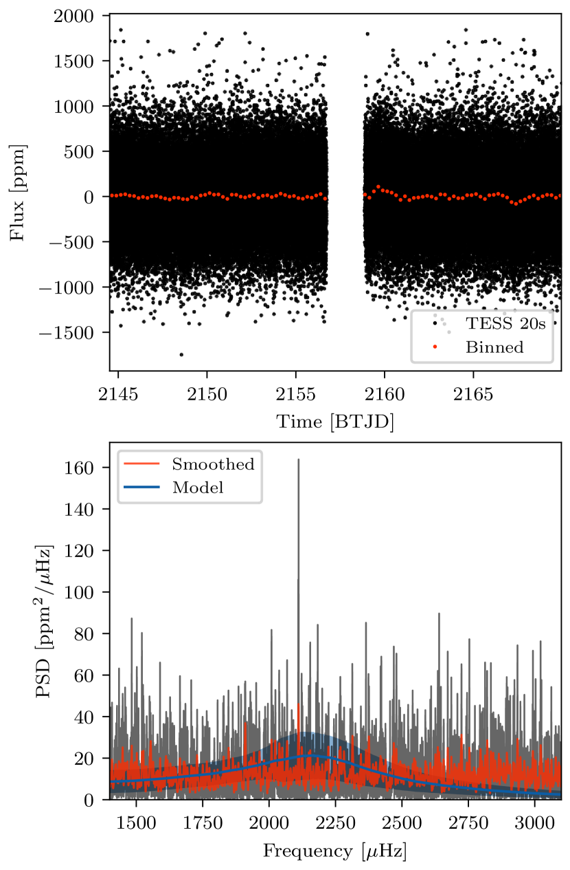
The top panel of Figure 1 shows the TESS 20-second cadence light curve for HD 19467. We observe no significant long-term variability, with an RMS of 25.5 ppm over 6 hour timescales. To search for high-frequency variability, we used the established asteroseismic tools pySYD (Huber et al., 2009; Chontos et al., 2021) and FAMED (Corsaro et al., 2020), which analyze the data in the frequency domain. Both methods detected a significant power excess near $\approx$ 2200 $\mu$Hz, consistent with the expected $\approx$7 minute timescale of solar-like oscillations (Bedding, 2014; García & Ballot, 2019) based on the spectroscopic temperature and surface gravity (Table 2). We also analyzed the data in the time-domain using a Gaussian Process (GP) model with a stochastically driven damped harmonic oscillator (Foreman-Mackey et al., 2017), which has been demonstrated to outperform traditional frequency analysis tools in recovering low S/N oscillations (Hey et al., in prep). The GP analysis strongly favored a model with an oscillating component with a $\Delta$BIC=7.1.

The bottom panel of Figure 1 shows the power spectrum of the 20-second light curve centered on the power excess. Solar-like oscillations are described by a frequency of maximum power ($\nu_{\textrm{max}}$) and a large frequency separation ($\Delta\nu$), which approximately scale with $\log g$ and the mean stellar density, respectively (Ulrich, 1986; Brown et al., 1991). We derive $\nu_{\textrm{max}}=2180\pm 100$ $\mu$Hz, with the central value taken from the median of three solutions (pySYD, FAMED, GP), and uncertainties calculated from the scatter over individual methods (e.g. Huber et al., 2013). The low S/N of the detection precludes an unambiguous detection of $\Delta\nu$. Visual inspection of an echelle diagram indicates $\Delta\nu\approx 101$$\mu$Hz, consistent with the derived $\nu_{\textrm{max}}$value.

Figure 1: Top: TESS Sector 31 light curve of HD 19467. Black points show the original 20-second cadence data, red points show the data binned to a timescale of 6 hours. Bottom: Power spectrum of the data centered on the detected power excess near $\approx$ 2200 $\mu$Hz. The blue line and filled area shows the median and standard deviation of the GP model posterior

3.2 Physical Properties of HD 19467

Table 2: Observations of the Host Star HD 19467

Property	Value	Units	Comments
Spectral Type	G3V		Gomes da Silva et al. (2021)
Teff	5720$\pm$10	K	Gomes da Silva et al. (2021)
Teff	5747$\pm$25	K	Brewer et al. (2016)
Teff	5770$\pm$80	K	Maire et al. (2020)
Teff	5742$\pm$10	K	Nissen et al. (2020)
Mass	0.953$\pm$0.022	M⊙	Maire et al. (2020)
Mass	0.960$\pm{0.02}$	M⊙	This work ($\S$3.2)
Age	5.41${}^{+1.8}_{-1.34}$	Gyr	Brandt et al. (2021a)
Age	8.0${}^{+2.0}_{-1.0}$	Gyr	Maire et al. (2020, Table 1)
Age	10.06${}^{+1.16}_{-0.82}$	Gyr	Wood et al. (2019)
Age	11.882$\pm{2.564}$	Gyr	Gomes da Silva et al. (2021)
Age	9.4$\pm{1.0}$	Gyr	This work ($\S$3.3)
$[$Fe/H$]$	$-$0.11$\pm$0.01	dex	Maire et al. (2020)
$[$Fe/H$]$	$-$0.09$\pm{0.04}$	dex	This work ($\S$3.2)
log(g)	4.32$\pm$0.06	cgs	Maire et al. (2020)
log(g)	4.28$\pm{0.04}$	cgs	This work ($\S$3.2)
R.A. (Eq 2000; Ep 2000)	03h07m18.570s		Gaia DR3
Dec. (Eq 2000; Ep 2000)	$-$13o45′42.419″		Gaia DR3
Distance	32.03$\pm$0.03	pc	Gaia DR3
Proper Motion ($\mu_{\alpha},\mu_{\delta}$)	($-$8.694, $-$240.64)	mas/yr	Gaia DR3
RUWE	1.0566		Gaia DR3
G	6.814$\pm$0.003	mag	Gaia DR3
H	5.447$\pm$0.033	mag	2MASS
W1 [3.4 $\mu$m]	5.36$\pm$0.16	mag	WISE
W2 [4.6 $\mu$m]	5.18$\pm$0.06	mag	WISE

We adopted the effective temperature ($T_{\rm eff}$) and metallicity ($\rm{[M/H]}$) from Brewer et al. (2016), derived from a line-by-line analysis of a Keck/HIRES spectrum. Literature values from spectroscopy and Gaia color-temperature relations (Casagrande et al., 2021) are highly consistent, with a range of 40 K in $T_{\rm eff}$ and 0.04 dex in iron abundance (Table 2). We used these ranges as an estimate for uncertainties, resulting in $T_{\rm eff}=5747\pm 40$ K and $\mbox{$\rm{[M/H]}$}=-0.09\pm 0.04$ dex. These uncertainties are smaller than those recommended by Tayar et al. (2022), which is justified by the fact that star has properties similar to the Sun and thus suffers from smaller systematic errors.

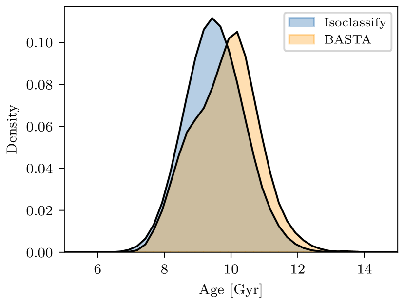
We then combined the asteroseismic $\nu_{\textrm{max}}$ measurement, Gaia DR3 parallax, 2MASS K-band magnitude, $T_{\rm eff}$ and $\rm{[M/H]}$ with isoclassify (Huber et al., 2017) and BASTA (Aguirre Børsen-Koch et al., 2022), which perform Bayesian inference of stellar parameters given input observables using the stellar evolution models MIST (Choi et al., 2016) and BASTI (Pietrinferni et al., 2004), respectively. Importantly, $\nu_{\textrm{max}}$  tightly constrains the surface gravity to $\mbox{$\log g$}=4.28$, which combined with the radius constraint from the Gaia parallax provides a tight constraint on stellar mass, which in turn constrains stellar age. Both tools consistently imply a mass of $\approx$ 0.95 $\,M_{\sun}$, which, given that the star has slightly evolved off the main-sequence (1.2$\,R_{\sun}$), implies an old age. Figure 2 shows the age posteriors from both evolutionary models and methods.

The final stellar parameters adopted in our study are listed in Table 3. We adopt the self-consistent solution derived from isoclassify, but add in quadrature the difference to the BASTA results to account for systematic errors due to different model grids (Tayar et al., 2022).

Figure 2: Posterior distributions for the age of HD 19467 based on isochrone modeling with isoclassify (blue) and BASTA (orange) using constraints from asteroseismology, spectroscopy and Gaia.

3.3 The Age of HD 19467

The age of HD 19467 is important for interpreting the mass and atmospheric composition of the brown dwarf companion. As already mentioned, literature estimates have a significant spread, ranging from 5–12 Gyr (Table 3). Younger, Sun-like ages come from stellar rotation (Maire et al., 2020) and activity (Brandt et al., 2021a), while older ages are preferred by isochrone fitting (Wood et al., 2019; Maire et al., 2020). The rotation-age is based on the detection of photometric period of $\approx$ 29 days with an amplitude of $\approx$ 0.5% from ground-based ASAS data (Maire et al., 2020). The high-precision of TESS light curve in Figure 1 rules out rotational modulation at the level of 0.5% over 25 day timescale suggested by the ASAS data, which implies that the rotation period for HD 19467 is undetermined. This is consistent with results from the Kepler Mission, which demonstrated that typical rotational amplitudes in mature Sun-like stars are on the order of a few hundred ppm (McQuillan et al., 2014; Santos et al., 2021) and thus are generally not detectable using ground-based photometry. Chromospheric activity-based ages also become more challenging for stars with Sun-like and older ages due the flattening of the age-activity relation, making age constraints sensitive to small changes in $R^{\prime}_{HK}$ measurements. While some literature values for $R^{\prime}_{HK}$ favor near solar values (and thus ages) for HD 19467, others are consistent with older, isochrone-based ages (e.g. $R^{\prime}_{HK}=5.1$ and $8.8\pm 0.3$ Gyr, Lorenzo-Oliveira et al., 2018).

The asteroseismic detection from TESS supports an older age for HD 19467. While the low S/N precludes a direct age from a measurement of individual oscillation frequencies (e.g. Mathur et al., 2012; Metcalfe et al., 2014; Silva Aguirre et al., 2017), the $\nu_{\textrm{max}}$ measurement precisely constrains $\log g$ and thus stellar mass independent of stellar evolutionary models. With a mass similar to solar ($0.96\pm 0.02$$\,M_{\sun}$), HD 19467 must have an age significantly older than the Sun to reach a radius of 1.2$\,R_{\sun}$. As discussed by Maire et al. (2020), an age of $9.4\pm 1.0$ Gyr is compatible with the slight enhancements in alpha elements and sub-solar metallicity, placing the star in the transition region between chemical “thin-disk” and “thick-disk” stars. Overall, we conclude that HD 19467 is an $\approx$4-5 Gyr older analog to our Sun and adopt an age of 9.4$\pm$1.0 Gyr (Table 3).

Table 3: Adopted Stellar Parameters for HD 19467A

Effective temperature, $T_{\rm eff}$  (K)	$5747\pm 40$
Metallicity, $\rm{[M/H]}$ (dex)	$-0.09\pm 0.04$
Luminosity, $L$ ($\,L_{\sun}$)	$1.42\pm 0.06$
Stellar radius, $R_{\star}$ ($\,R_{\sun}$)	$1.20\pm 0.03$
Stellar mass, $M_{\star}$ ($\,M_{\sun}$)	$0.96\pm 0.02$
Stellar density, $\rho_{\star}$ (cgs)	$0.56\pm 0.03$
Surface gravity, $\log g$ (cgs)	$4.28\pm 0.04$
Age, $t$ (Gyr)	$9.4\pm 1.0$

4 NIRCam Data Reduction and Post Processing

We use the processed images retrieved from the Mikulski Archive for Space Telescopes (MAST) that have been corrected for bad pixels, flat-fielding, and background subtraction with the jwst pipeline. The product we use are the calints files which result from Stage 2 of the pipeline and have been through a photometric calibration. The data were processed with calibrations software version 1.5.3 and calibration reference data context jwst_0943.pmap. In addition to these data, we take advantage of wavefront information provided by Optical Path Difference (OPD) maps taken by the NIRCam wavefront sensing team to generate a NIRCam PSF model close in time to our science observations. For synthetic PSFs, we utilize the OPD from 2022-08-11, R2022081102-NRCA3_FP1-1.fits, the closest in time preceding our observations.

4.1 PSF Subtraction

We apply principal component analysis (PCA) (e.g. Lafrenière et al., 2007; Amara & Quanz, 2012) via Karhunen Loéve Image Projection (KLIP; Soummer et al., 2012), to subtract the residual stellar intensity from the science frames using the images taken in two roll angles for angular diversity. We perform PSF subtraction using the open source Python package pyKLIP (Wang et al., 2015) using Angular Differential Imaging (ADI) and Reference Differential Imaging (RDI) using a synthetic reference PSF, as described below. The results of the PCA reduction for all filters is displayed in Figure 3.

Figure 3: Post-processed images of HD 19467 in the six NIRCam filters observed in this program, rotated so that North is up. Images were reduced using the pyKLIP algorithm as described in the text. Arrows indicate the detected companion.

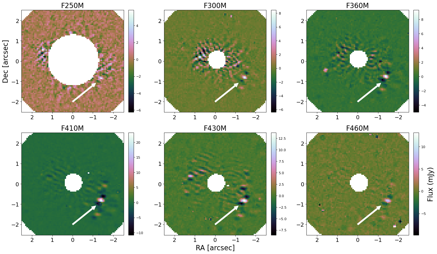
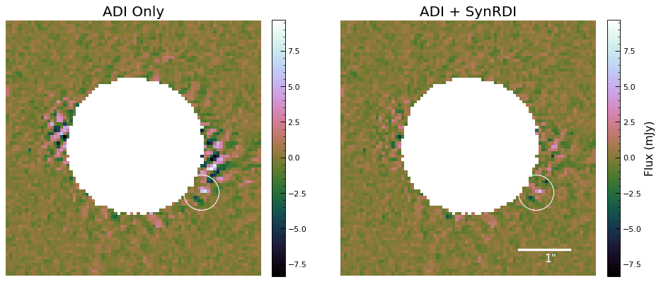
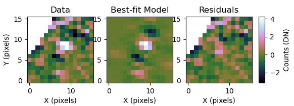
For all filters except filter F250M, the data contained in the two rolls suffices to obtain an unambiguous detection of the companion. For the F250M case, although the companion’s signal is visible using only ADI, we resorted to using RDI with a set of synthetic PSFs in order to confirm the signal is indeed from the companion and not due to residual speckles. In Figure 4 we show the comparison, for the F250M filter, between only using the roll frames for the PCA reduction (ADI), and assisting the PCA reduction with a set of synthetic PSFs (ADI+SynRDI).

Figure 4: Top: Comparison between using only ADI for the PCA reduction (left), and using RDI with synthetic PSFs generated with WebbPSF (right) for the the F250M data. The addition of RDI reduces the speckle noise in the PSF-subtracted images. The data are oriented so that North is up. Bottom: The forward model compared with the PSF-subtracted data for F250M, using the sythetic PSFs as reference.

The grid of synthetic stellar PSFs is generated using WebbPSF (Perrin et al., 2014) and tools from webbpsf_ext at offset locations with respect to the coronagraph focal plane mask. We generate simulated PSFs in different sets of 9-point grid pattern at even spacings. We simulate spacings of 2.5, 7, 15, 25, 40 mas, in addition to a set of rotations of the coronagraphic-PSF with respect to the detector of 0.1, 0.3, 0.5 degrees. This aims to emulate the speckles present in the data frames, and assists the PCA reduction with the diversity in speckle structure needed to perform a more optimal reference subtraction.

As mentioned above, for filters F300M, F360M, F410M, F430M, and F460M, ADI suffices for a clear detection. As a second step we use RDI with the synthetic PSFs to further subtract the unwanted starlight. This is motivated by the fact that the companion PSF’s northern lobe falls near the diffraction speckles caused by the bar coronagraph. The number of Karhunen Loéve (KL) modes determines how much of the synthetic PSFs are used for the subtraction. Since these have been generated with arbitrary offsets, there is a risk of subtracting the light from the secondary. We use 15 KL modes, which minimizes over-subtraction and clears out slightly more of the residual starlight around the northern lobe. This was done by visual inspection; a more in-depth analysis on how to optimally use synthetic PSFs will be explored in the future.

4.2 Photometry

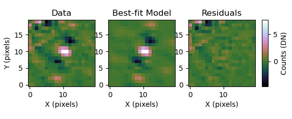
To accurately extract the flux and position of HD 19467 B, we account for over-subtraction effects on the PSF that arise during the reduction process (described in Section 4.1) with a forward model based on the method described by Pueyo (2016). We make use of its implementation on pyKLIP (Wang et al., 2015). The companion PSF is modeled using WebbPSF (Perrin et al., 2014) for each filter and accounting for its position with respect to the bar focal plane mask. An accurate position of the simulated PSF is particularly important in the case of the shorter wavelength filters: poorer spatial sampling of the pixels compared to the diffraction limit at smaller wavelengths (2.5$\rm\,\mu m$ is sub-Nyquist) results in an acute sensitivity of the PSF structure as seen in the detector. An accurate positioning for the case of F250M was done by trial and error simulating a grid of PSF offsets and selecting the best fit by least square difference between the simulation and the coadded science frames. The model PSF are simulated using the OPD map closest in time and prior to the observations.

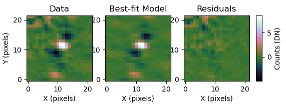
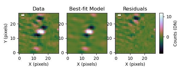
The flux and position of the companion are extracted with pyKLIP. We fit a model of its photometry and astrometry to the reduced data using an MCMC approach (emcee; Foreman-Mackey et al. (2013)). Figure 5 shows the PSF model fit to the reduced data for filter F360M, the filter in which we obtain the highest SNR. Appendix A contains the full gallery of forward model comparisons with the PSF-subtracted images in each band.

Figure 5: The best fit model to the PSF-subtracted signal used to measure the photometry and astrometry of HD 19467 B in filter F360M, where the highest SNR was achieved. The residuals show the companion is fit well by the forward model.

The flux calibration of the signal is determined based on the jwst stage 2 pipeline photometric calibration. We apply a flux correction to the photometry based on measured attenuation factor of $0.92$ of the Bar mask Lyot stop at $\sim 1.6$″. We fit a G3V stellar photosphere model to 1-5 $\rm\,\mu m$ photometry from 2MASS (Cutri et al., 2003) and WISE (Cutri & et al., 2012). We also find a $\sim 2\%$ error in fitting the stellar model to the IR measurements, and apply this error to contrast reported. Table 4 shows the estimated stellar flux. Comparison of the calibrated flux measured from the acquisition and astrometric confirmation images, both taken through the neutral density square, produced from the stage 2 pipeline is consistent with the estimated stellar spectrum within $\sim 10\%$. We therefore apply a $10\%$ uncertainty to reported absolute photometry of HD 19467 B in this section.

Table 4: Adopted Photometry For HD 19467 A

Filter	Flux (Jy)
F250M flux (Jy)	3.51$\pm$0.07
F300M flux (Jy)	2.63$\pm$0.05
F335M flux (Jy)	2.10$\pm$0.04
F360M flux (Jy)	1.82$\pm$0.04
F410M flux (Jy)	1.49$\pm$0.03
F430M flux (Jy)	1.36$\pm$0.03
F460M flux (Jy)	1.12$\pm$0.02

Figure 6 shows the measured photometry in each NIRCam band alongside recent measurements and limits from the ground (Mesa et al., 2020; Maire et al., 2020). The F460M flux is consistent with the M band upper limit obtained with VLT NaCo Maire et al. (2020), however there appears to be some tension with the NaCo L’ flux compared with F360M and F410M photometry measurements. Carter et al. (2022) also noted a discrepancy in measurements from NaCo $L^{\prime}$ and JWST NIRCam photometry. The difference in passband on a steeply rising part of the spectrum, possible water vapor effects, as well as calibration uncertainties may account for this discrepancy. Continued refinement of JWST photometric calibrations will help identify any biases in photometry. For this study, we do not incorporate NaCo photometry into the analysis, but rather present the measurement comparison for future investigation.

Figure 6: New NIRCam photometry (blue stars) compared with recent ground-based measurements from VLT-SPHERE and VLT-NACO.

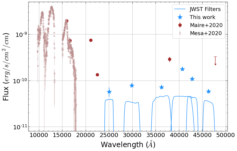
Table 5 shows our measured photometry and relative astrometry for HD 19467 B (see next section).

Table 5: NIRCam measurements of HD 19467 B 

	Separation	Pos. Angle	$\Delta$mag	Flux
Filter	(″)	(deg)	(mag)	($\mu$Jy)
F250M	1.597$\pm$0.010	236.9$\pm$0.14	13.67$\pm$0.271	11.96$\pm$2.75
F300M	1.611$\pm$0.002	237.2$\pm$0.04	12.62$\pm$0.122	23.50$\pm$2.52
F360M	1.610$\pm$0.003	236.9$\pm$0.07	11.91$\pm$0.127	31.41$\pm$3.58
F410M	1.604$\pm$0.001	236.8$\pm$0.04	10.45$\pm$0.116	98.74$\pm$10.20
F430M	1.609$\pm$0.003	236.6$\pm$0.07	10.78$\pm$0.124	66.32$\pm$7.35
F460M	1.609$\pm$0.003	236.9$\pm$0.07	11.07$\pm$0.121	41.78$\pm$4.64

Note. — $T_{\rm eff}$ and $\rm{[M/H]}$ are adopted from Brewer et al. (2016), with uncertainties accounting for the spread in literature results. All other properties are derived from the combination of constraints from asteroseismology, spectroscopy and Gaia (see §3).

Note. — Predicted fluxes in JWST wavebands are based on BOSZ stellar models (Bohlin et al., 2017).

Note. — NIRCam astrometry and photometry from 2022-Aug-12

Note. — The astrometric precision for each filter is based solely on the positional uncertainty relative to the center of the coronagraph mask. The combined astrometry includes an additional term to account for uncertainty in the stellar position behind the mask (7 mas in each direction).

4.3 Relative Astrometry

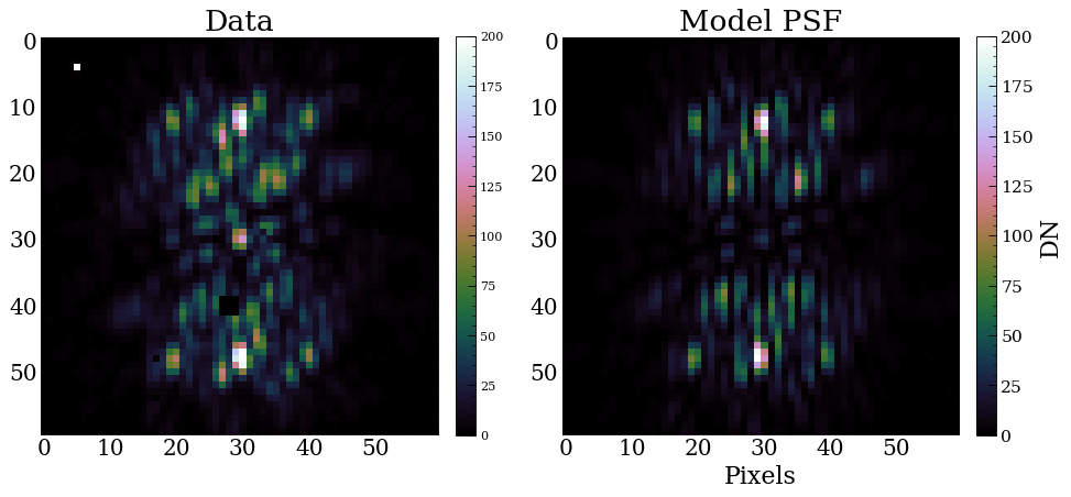
A major challenge of obtaining relative astrometry of a companion in coronagraphic imaging is that the primary star is occulted by the focal plane mask. Knowledge of the wavefront from published OPD maps, and a highly structured PSF enable a forward model based cross-correlation with the data to fit for the centroid of the star behind the mask. We perform a cross-correlation of model PSFs with the data using the chi2_shift in the image-registration Python package to measure the best fit position of the star behind the mask (Figure 7). We obtain a centroiding error $\sim$7 $\mathrm{mas}$, consistent with the measured sensitivity in Carter et al. (2022).

Figure 7: Left: An example of the raw MASKLWB coronagraph data for an image in the F360M filter. Right: The best fit model PSF simulated using the most recent preceding OPD map, used to measure the centroid of the star.

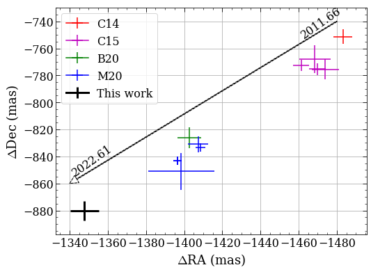
The companion position is recovered with the joint astrometry and photometry model fit to the reduced data as described in Section 4.2. The model fit errors provide the uncertainty in the relative position to the measured star position on the detector. We add the star position uncertainty to the reported errors (Table 5). Figure 8 shows the new astrometric measurement compared to previous relative astrometry measurements of HD 19467 B (Crepp et al., 2014, 2015; Bowler et al., 2020; Maire et al., 2020).

Figure 8: Astrometric position of HD 19467 B relative to its parent star, compared with previous measurements.

4.4 Performance and Sensitivity

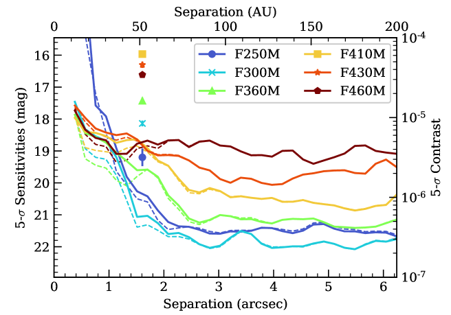
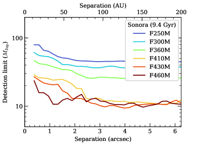
In Figure 9 we show the contrast curves for the reduced images after PSF subraction. The contrast is measured with PyKLIP by computing the noise in an azimuthal annulus at each separation, using a Gaussian cross correlation to remove high frequency noise. The flux normalization to obtain these contrast numbers was computed as explained in Section 4.2, by using a best fit model of the stellar spectrum to calibrate contrast. The contrast curves are corrected for algorithmic throughput, i.e. the throughput loss due to the PSF subtraction, and for small sample statistics (Mawet et al., 2014).

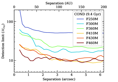
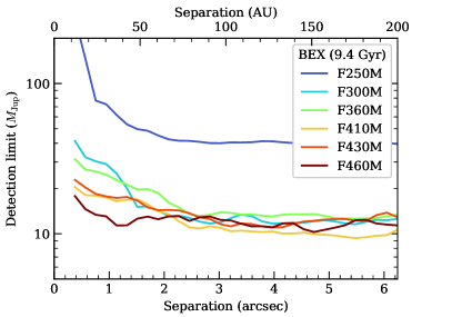
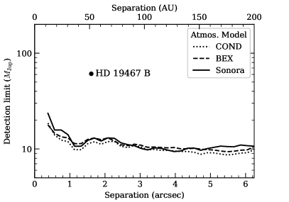
Figure 10 translates our detection limits from flux/contrast sensitivities to limits on companion mass. Three different brown dwarf evolution models are considered – Ames-COND (Baraffe et al., 2003), BEX-HELIOS (Linder et al., 2019), and Sonora-Bobcat (Marley et al., 2021). In each case, we assume solar metallicity.

While the shortest wavelength observations achieve the best contrast (in particular F300M), the longer wavelengths are better at detecting lower mass companions. We find an overall detection limit of $\sim$10 $\,M_{\rm J}$. This limit is much higher than the sub-Jupiter levels that JWST/NIRCam can obtain for young systems (e.g. Carter et al., 2022), but even for this very old system brown dwarfs are easily detectable outside of $\sim$0.4″ $\simeq$ 10 AU. While the detection limit is relatively independent of model, it does depend significantly on the age of the brown dwarf (the system age is discussed in §3.3).

Figure 9: Contrast curves for all filters. Solid lines indicate ADI, and dashed lines indicate ADI and RDI using synthetic PSFs. Data points indicate the HD 19467 B detections. The use of synthetic PSFs provides the diversity necessary to obtain enhanced contrast at small angular separations.

Figure 10: Detection limits ($5-\sigma$) for each filter, in terms of companion mass. The first three panels show limits for three different atmospheric evolution models (COND, Bex, and Sonora), while the last panel compares the overall detection limit for each of the models. A mass estimate from atmospheric model fitting (Section 6) is shown as a point in the lower right figure (61 $\,M_{\rm J}$ at 1.61″).

Despite a lack of reference star observations, we are able to recover the signal of HD 19467 B with two roll angles and achieve contrasts $\sim$10^-5 at 1–2 arcsec. Regular OPD measurements enable the use of synthetic PSFs that can aid PSF subtraction by generating a set of reference PSFs to capture speckle structure. This suggests that bright companions could be observed without reference stars, significantly reducing the time spent on the observation. Future work will investigate the difference between reducing data with and without reference star observations. Future observations with a better defined position for the LWB coronagraph should also provide better contrast close-in.

5 Orbit of HD 19467 B

Previous studies estimate the mass of HD 19467 B from 51 to 86$\,M_{\rm J}$ through both model-based estimates and orbital analyses (Crepp et al., 2014; Maire et al., 2020; Brandt et al., 2021a). We analyze new radial velocities and provide an updated dynamical mass estimate including our new relative astrometry and additional RV measurements.

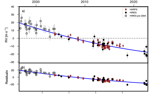
First, we fit the new and previously measured RVs from HIRES and HARPS (Trifonov et al., 2020) using the RadVel software (Fulton et al., 2018). With the addition of the new data, we measure a linear slope term of $\dot{\gamma}=-0.00412\pm 0.00027$ m s^-1 d^-1 with strong significance. We attempt to fit for curvature and tentatively detect a curvature term of $\ddot{\gamma}=1.7^{+0.81}_{-0.78}\times 10^{-7}$ m s^-1 d^-2 at 2.1$\sigma$. Model comparison using $\Delta BIC$ and $\Delta AIC$ (Aikike Information Criterion, Burnham & Anderson (2002)) show a nearly indistinguishable model fit to a trend-only and trend plus curvature model. A detection of curvature can place strong constraints on the companion orbit, especially for higher eccentricity systems. Figure 11 shows the RV data plotted over the maximum likelihood model. Appendix 2.2 contains a more detailed description of the fit comparison and the new radial velocities used in the analysis.

Figure 11: Best fit single companion Keplerian orbital model for HD 19467 to radial velocities measured for HD 19467 by HIRES by the California Legacy Survey (Rosenthal et al., 2021), new HIRES observations, and HARPS (Trifonov et al., 2020). The fit slightly favors a curvature term.

For the full orbital analysis we include all available RV measurements from HARPS (Trifonov et al., 2020) and HIRES (HIRES data including new measurements tabulated in Appendix B), relative astrometry (Crepp et al., 2014, 2015; Bowler et al., 2020; Maire et al., 2020) (listed in Table 6), and absolute astrometry from Hipparcos and Gaia as described in Brandt et al. (2021a), which takes advantage of proper motion anomalies between Hipparcos, Gaia EDR3 and the Hipparcos-Gaia long-term trend. We utilize the cross-calibrated catalog of Hipparcos-Gaia accelerations presented in Brandt (2021).

Table 6: Imaging Astrometry

epoch$-2450000$	Filter	$\rho$ (mas)	$\rho_{err}$	PA (deg)	PAerr
Astrometry from Crepp et al. (2014)
5804.1	K’	1662.7	4.9	243.14	0.19
5933.8	H	1665.7	7.0	242.25	0.26
5933.8	K’	1657.3	7.2	242.39	0.38
6166.1	K’	1661.8	4.4	242.19	0.15
6205.0	Ks	1653.1	4.1	242.13	0.14
Astrometry from Maire et al. (2020)
8032.3	L’	1637	19	238.68	0.47
8061.2	K1	1636.7	1.8	239.39	0.13
8061.2	K2	1634.4	5.0	239.44	0.21
8409.3	H2	1631.4	1.6	238.88	0.12
8409.3	H3	1631.4	1.6	238.88	0.12
New Astrometry (this work; see Table 5)
9803.9	2.5–4.6$\mu$m	1607.6	7	236.84	0.25

We use orvara (Brandt et al., 2021b) to fit orbits to the radial velocities, absolute astrometry, and relative astrometry. orvara is an orbit fitting code that uses ptemcee, a parallel tempered MCMC scheme (Foreman-Mackey et al., 2013; Vousden et al., 2016). Following the orbital analysis in Brandt et al. (2021a), we apply a geometric prior to inclination and log-flat priors to semi-major axis and companion mass. We apply uniform priors to remaining orbital elements. log-flat priors are applied to RV jitter. We adopt the mass of $M_{*}=$ 0.96 $\pm 0.02~{}\,M_{\sun}$ based on the analysis in §3 using asteroseismology, spectroscopy, and Gaia data.

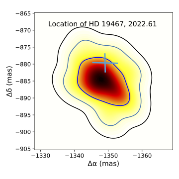
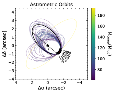
We first predict the position of HD 19467 B in the current epoch leaving out the new relative astrometry measured with NIRCam, but including all other data. Figure 12 shows that our measurement is consistent with the prediction of the best fit orbits using previous measurements.

Figure 12: Orvara prediction of relative astrometry at the 2022-08-12 epoch. The measured astrometry is consistent with the prediction.

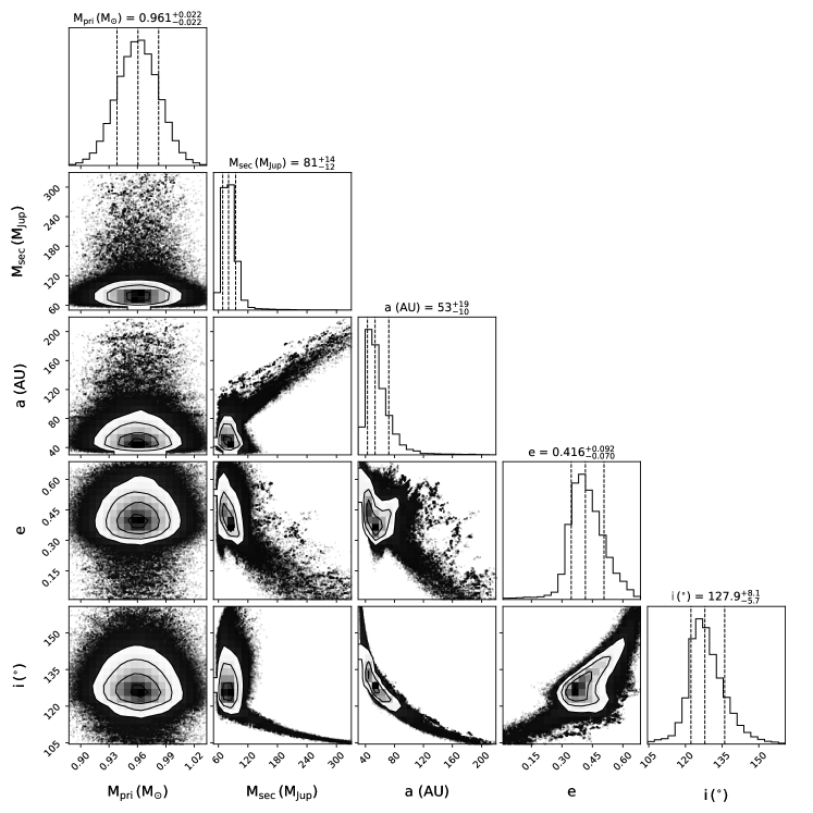
Next, we fit for orbital parameters including our new relative astrometry measurement from NIRCam. Table 7 summarizes the orbit fit results. We infer a mass of $81^{+14}_{-12}$$\,M_{\rm J}$. Our mass estimate for HD 19467 B is within 1-$\sigma$ of the prior estimates from in Brandt et al. (2021a) ($65.4^{+5.9}_{-4.6}$$\,M_{\rm J}$), and Maire et al. (2020) ($74^{+12}_{-9}$$\,M_{\rm J}$). We infer an eccentricity of $0.416^{+0.092}_{-0.07}$, which is consistent with recent measurements in Brandt et al. (2021a), $0.54\pm 0.11$, Maire et al. (2020), $0.56\pm 0.09$, and Bowler et al. (2020), $0.39^{+0.26}_{-0.18}$. We infer a period of $386^{+220}_{-108}$ yr, which is consistent with prior orbital analyses (Bowler et al., 2020; Maire et al., 2020; Brandt et al., 2021a). The tentative evidence for curvature from the new radial velocities may indicate that the orbit is close to periastron passage. Given the high eccentricity, it could be a critical time to monitor this system.

Figure 13 shows a selection of orbits from MCMC posteriors overlaid with the relative astrometry used in the fit, and Figure 14 displays a corner plot of the MCMC posteriors for orbital parameters.

Figure 13: A selection of orbits from the MCMC posteriors.

Figure 14: Corner plot showing MCMC posteriors for select orbital parameters.

Table 7: Orbit fit results

Parameter	Units	Value
Jitter	m/s	${3.17}_{-0.23}^{+0.25}$
$M_{pri}$	$M_{*}$	${0.961}_{-0.022}^{+0.022}$
$M_{sec}$	$\,M_{\rm J}$	${81}_{-12}^{+14}$
Semi-major Axis	AU	${53}_{-10}^{+19}$
$\sqrt{e}\sin\omega$		${-0.586}_{-0.061}^{+0.068}$
$\sqrt{e}\cos\omega$		${0.08}_{-0.32}^{+0.29}$
Inclination	deg	${127.9}_{-5.7}^{+8.1}$
Ascending Node	deg	${48.9}_{-7.3}^{+240}$
Mean Longitude	deg	${192.7}_{-123}^{+7.7}$
Parallax	mas	${31.226}_{-0.037}^{+0.037}$
Period	year	${382}_{-108}^{+220}$
Argument of Periastron	deg	${278}_{-29}^{+27}$
Eccentricity		${0.416}_{-0.070}^{+0.092}$
Semi-major Axis	mas	${1664}_{-328}^{+598}$
$T_{0}$	JD	${2486667}_{-4207}^{+51547}$
Mass Ratio		${0.080}_{-0.012}^{+0.014}$

6 Atmosphere and Evolution Model Comparison

In the following sections we show a preliminary comparison of our near-IR photometry from NIRCam with brown dwarf atmospheric models, focusing on the Sonora models (Marley et al., 2021; Karalidi et al., 2021). In our spectral fitting, we only use the model spectral grid with solar carbon-to-oxygen ratio.

The Sonora-Bobcat cloudless atmospheric models assume that the atmospheric composition is in thermo-chemical equilibrium and solve radiative transfer equations for a self-consistent temperature-pressure profile. The model grid covers temperatures from 200 to 2400 K, gravity from 10 to 3160 $\rm m\,s^{-2}$, and metallicities from [Fe/H]=-0.5 to 0.5. The model spectra have a spectral resolution ranging from 0.6 to 20$\rm\,\mu m$ .

The Sonora-Cholla cloudless models assume chemical disequilibrium. These models assume that atmospheres have solar metallicity (Lodders, 2010) with cloud-free atmospheric structures. The models are computed using the Picaso v3.0 atmospheric model (Mukherjee et al., 2022). By including an eddy diffusion parameter, $K_{\rm zz}$, that ranges from $10^{2}-10^{7}\,\rm cm~{}s^{-2}$ as an input parameter, the Cholla models simulate the dynamical mixing that drives various molecular species like CH₄, CO, H₂O, and NH₃ out of their thermochemical equilibrium abundances. The Cholla models span over a temperature grid of 500 to 1300 K and a gravity grid from 56 to 3160 $\rm\,cms^{-2}$.

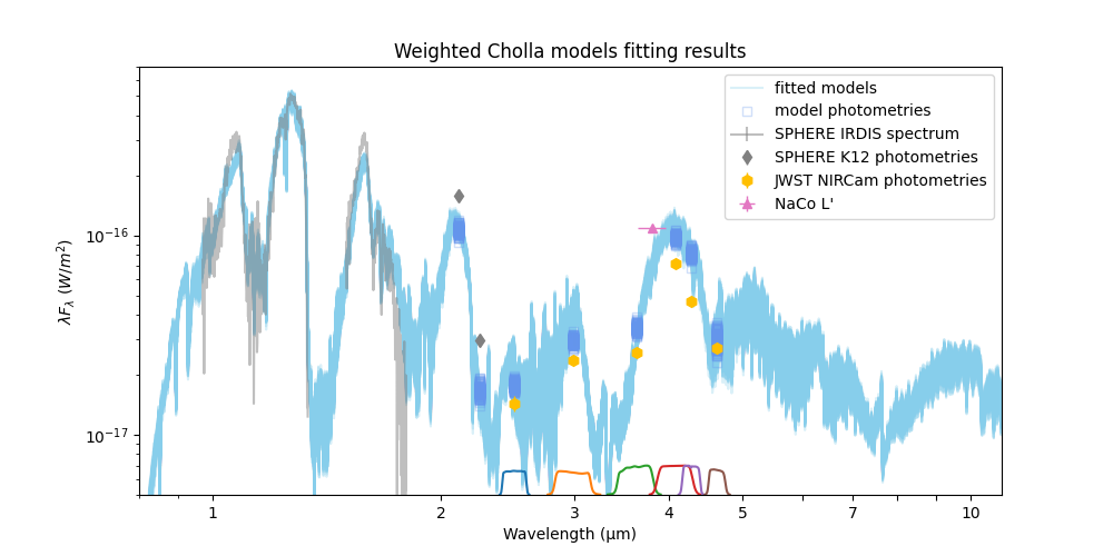
First, we perform a basic $\chi^{2}$ comparison of new JWST photometry to the Sonora models (Marley et al., 2021; Karalidi et al., 2021). We also perform an MCMC fit of the model grids with both our new photometry and previously published medium resolution spectrum obtained with SPHERE-IRDIS LSS (Mesa et al., 2020) and ground-based photometry from SPHERE-IRDIS Maire et al. (2020). From this we derive a bolometric luminosity and determine model-dependent mass estimate.

6.1 Model Comparison with NIRCam Photometry Only

We compare the NIRCam photometry with both the Sonora-Bobcat and Sonora-Cholla model grids to highlight the broad features of the $2-5\,\rm\mu m$ flux. We allow the radius scaling to vary when fitting the models to our NIRCam photometry, which is generally consistent with radii much smaller than, e.g., those predicted by the Sonora-Bobcat grid evolutionary tables.

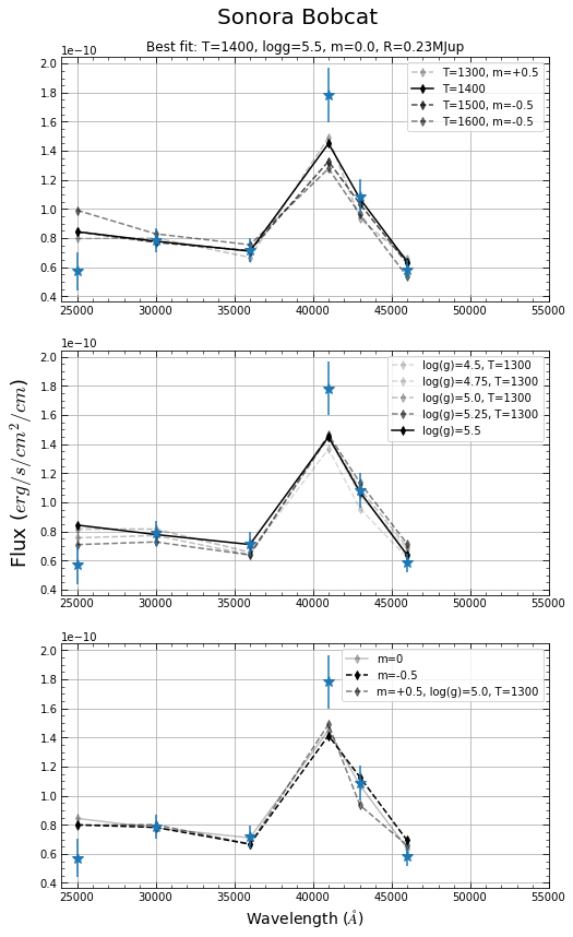
We find that the Bobcat models do not simultaneously capture both the local flux peak at $3\,\rm\mu m$ and the steep drop in flux from $4-5\,\rm\mu m$. In general the Bobcat grid favors higher gravity and lower or zero metallicity. However, none of the fits capture all of the photometry perfectly. A model spectrum at effective temperature of $T_{eff}=1400K$ best matches the data, but does not fully capture the peak flux at $\sim 4\,\rm\mu m$ with the drop off at longer wavelength. Gravity and metallicity do not have a strong effect on the fit.

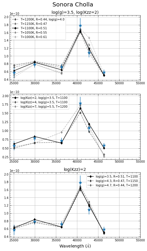
The Sonora Cholla models, which include effects of disequilibrium chemistry, provide better fits to the photometry, but suggest a low value for gravity as well as small radius to scale the flux. The best fit model has $T_{eff}=1200K$, $g=31$, and $log(K_{zz})=2$. Figure 15 (right) shows the best fitting Cholla model, with a few model grid points that vary in temperature, eddy diffusion parameter, and gravity. We note that while lower gravity is favored, the gravity does not strongly affect the shape of the photometry-only profile, as can be seen in the third panel. Near-IR spectroscopy with JWST will be able to further distinguished features of gravity.

Overall, the best fit Sonora-Cholla model provides a better fit than the best fit Sonora-Bobcat model. As can be seen in Figure 15, the Cholla models are better able to simultaneously capture the lower flux at shorter wavelengths, the peak at $\sim$4 $\mu$m, and the subsequent drop in flux, favoring a lower temperature that is more consistent with previous estimates. This suggests that modeling disequilibrium chemistry may be necessary for understanding the atmosphere and evolution of HD 19467 B.

Figure 15: Left: Measured photometry from NIRCam plotted alongside a few closely matching scenarios from the Sonora-Bobcat models, letting the radius vary. Right: Measured photometry from NIRCam plotted alongside a few closely matching scenarios from the Sonora-Cholla models, which include chemical disequilibrium parameterized by the eddy diffusion parameter, $log(K_{zz})$.

6.2 Model Fit to 1-5 $\mu m$

We fit the Sonora-Cholla cloudless models to the composite dataset that consists of JWST photometry, the IRDIS spectra (Mesa et al., 2020), and the SPHERE K12 band photometry (Maire et al., 2020) to constrain the temperature and gravity of HD19487B. For the IRDIS spectra, we exclude spectral points with negative flux values. We include an additional uncertainty of 7%, similar to the J- and H-band absolute flux uncertainties of HD 19467 (Table 7 of Mesa et al. 2020), to account for the possible offset in the absolute flux levels.

We linearly interpolate the Cholla model spectral grid to a finer grid with smaller step sizes in the temperature, gravity, and eddy diffusion parameter. In addition to the three parameters, the other free parameter in the spectral fitting is the scaling factor, which is the square of the ratio of brown dwarf radius to the distance (32.03 pc). We use pyphot to calculate the broadband photometries of model spectra.

Our model fitting algorithm minimizes a cost function that sums the squared difference between the model spectra and data, weighted by the observational uncertainties, $\sigma$, and the intensities, $w$, as shown in the following:

$${\mathrm{c}ost~{}function}=\Sigma_{i=1}^{N}\{w_{i}\frac{F_{\lambda,i}(model)-F_{\lambda,i}(data)}{\sigma_{i}}\}^{2}\\ w_{i}=\frac{F_{\lambda,i}\Delta\lambda_{i}}{max(F_{\lambda,i}\Delta\lambda_{i})}$$ (1)

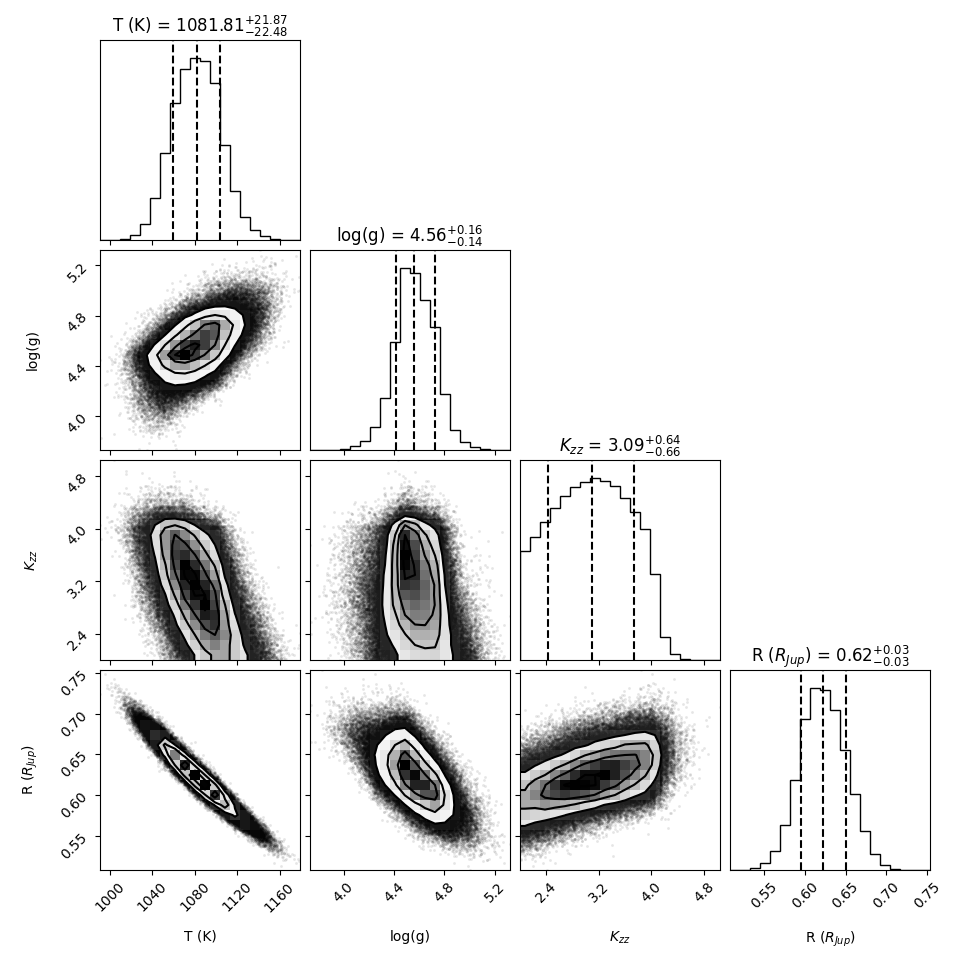
where $\Delta\lambda_{i}$ is the wavelength coverage of a datapoint and the intensity weighting is normalized by the highest intensity among the datapoints. We include the intensity weighting in the cost function so that a photometric point with high intensity carries more weight in the fitting process than a spectral point with low intensity even though both could have a similar signal-to-noise ratio, since the photometric points contain a larger fraction of total flux measured. We then use emcee (Foreman-Mackey et al., 2017) to sample the posterior distribution of the fitted parameters with the Markov Chain Monte Carlo (MCMC) method. We adopt a uniform prior of temperature, logarithmic gravity, and eddy diffusion parameter. We run the MCMC chain with 200 walkers for 20,000 steps. Based on the posterior distribution of the MCMC chains, we derive the best-fit temperature of $1080\pm 22{\rm\,K},$ gravity of $\log(g)=4.60^{+0.2}_{-0.1},$ eddy diffusion parameter of $\log K_{\rm zz}=3.1^{+0.6}_{-0.4}$, and radius R of $0.62\pm 0.03R_{\rm J}$. The value for radius is lower than the expected radius at 9 Gyr, $\sim$0.8 $\mathrm{R_{Jup}}$, according to the evolution model grid at similar parameters. Prior modeling work has noted a common discrepancy between the expected radius from evolutionary models and the radius required to match the flux of a given temperature that best fits atmospheric models (e.g., Barman et al., 2011; Marley et al., 2012; Lavie et al., 2017). Maire et al. (2020) explored radius agreement with evolutionary tracks with different model atmospheres that included various levels of clouds in the atmosphere. Future observations, especially spectroscopy will further help constrain atmospheric models.

We draw 100 parameter sets from the posterior distribution and plot the corresponding model spectra in Figure 16. Figure 16 suggests that the model spectra provide a qualitatively good match to the data but there are some significant residuals, especially in the $K$-band photometries. We remain cautious about the inferred parameters and the seemingly small uncertainties given the imperfect fit between the data and model spectra. However, while absolute flux calibration may account for some discrepancy between data sources, the discrepancy alone is not enough to account for inconsistencies between the best fit atmospheric model and evolutionary grid predictions. Clouds, which likely drive the rotational modulation of many T dwarfs (e.g Manjavacas et al., 2019) and are not included in the Cholla models, could play a key role in shaping the HD 19467 B emission spectra. Future simultaneous observation in the near-IR and mid-IR region will be useful for testing the role of clouds in the atmosphere of HD 19467 B with well-constrained age and host star metallicity.

Figure 16: The comparison of the fitted Cholla model spectra (light blue lines) to the SPHERE/IRDIS-LSS 1–1.8$\rm\,\mu m$ spectra (gray lines), SPHERE/IRDIS-K12 photometry (gray diamonds), NaCo L’ band (pink triangle), and JWST NIRCam photometry (golden hexagon) show that it is challenging for the models to simultaneously explain the near-IR and mid-IR spectra and photometry. The semi-transparent light blues lines are the 1000 Cholla cloudless model spectra sampled from the posterior distribution of MCMC fitting results. The blue squares are the effective photometry from the model spectra samples in the corresponding NIRCam filters. The transmission curves of JWST NIRCam broadband photometry are plotted in colored lines at the bottom of the plot. The y-axis is in unit of intensity ($\rm Wm^{-2}$).

6.3 Bolometric Luminosity

Figure 17: Based on the bolometric luminosity and age, the Bobcat evolution models suggest that HD 19467 B has a mass of $62\pm 1$ $\,M_{\rm J}$. The colors indicate the masses predicted by Bobcat evolution models. White contour lines show the bolometric luminosity and age with a fixed mass. The uncertainty of HD 19467 B’s bolometric luminosity is around 4%.

The 2-5µm JWST NIRCam broadband photometry, in combination with the ground-based near-infrared spectra and photometry, are crucial for pinning down the bolometric luminosity of a $\sim$1000 K object. We integrate the flux density over observed data including the previously published IRDIS-LSS spectra (0.97-1.335 $\mu$m & 1.50-1.80  $\mu$m) , ground-based K-band photometry (2.059-2.161 $\mu$m & 2.1965-2.3055 $\mu$m), and the six JWST NIRCam broad band photometry. The flux integral in the observed wavelength regions is $3.28\pm 0.2\times 10^{-6}L_{\odot}$.

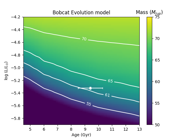
We utilize the fitted model spectra in Section 6 to extrapolate flux density beyond the observed wavelength region and estimate the bolometric luminosity. We find that the observational data accounts for around 72% of the bolometric luminosity. The estimated total bolometric luminosity is $(4.75\pm 0.2)\times 10^{-6}L_{\odot}$, or $\log(L/L_{\odot})=-5.32\pm 0.02$. Based on the combination of JWST NIRCam high-precision photometry and ground-based data, our results suggest that we can accurately derive the bolometric luminosity at 4% precision level.

Based on the independently estimated age and bolometric luminosity, we then use the Bobcat evolution model to estimate mass of HD 19467 B. After linearly interpolating the mass as a function of age and bolometric luminosity, we derive that the mass is $62\pm 1M_{J}$. Figure 17 shows the Sonora Bobcat evolution model and where our bolometric luminosity estimate lies. By comparing the mass derived from the age and $L_{bol}$ to the dynamical mass, ($81^{+14}_{-12}M_{J}$), we conclude that the two masses are consistent with each other within about two-sigma.

The NIRSpec IFU observations planned for later this year (PID #1414) will provide a much more complete characterization of the atmosphere of HD 19467 B, helping to pin down parameters such as metallicity and $T_{\rm eff}$.

7 Conclusions

We have demonstrated the performance of JWST NIRCam LWB coronagraph on the known binary system HD 19467 B. Despite missing reference star observations, we are able to recover the companion with high significance in all 6 medium NIRCam bands used for the observations.

The main results of this study are as follows:

• The MASKLWB coronagraph works well for separations below $1$ arcsec (for medium filters excluding F250M) at contrasts $10^{-5}$ and better, even without a reference star when angular diversity is utilized. This is expected to improve in the near future when coronagraphic mask locations are refined through instrument calibration observations.

• Given the superb stability of JWST, and regular OPD measurements available, we are able to incorporate synthetic reference images to further subtract speckles, following ADI subtraction, and improve SNR on the detections. Future observations with reference observations can be compared with the results presented in this study.

• We estimate the age of the HD19467 system by combining spectroscopy and Gaia astrometry with asteroseismic constraints from TESS, finding an age of $9.4\pm 1.0$ Gyr, supporting older estimates of the age. We provide updated parameters for the host star HD19467.

• We estimate a dynamical mass of HD 19467 B of $81^{+14}_{-12}M_{J}$, contributing new relative astrometry from NIRCam and radial velocities from HIRES, and detect tentative evidence of curvature in the orbit fit to the radial velocities.

• A comparison of atmospheric and evolutionary models to our new $2-5$ $\mu$m photometry favors models that include disequilibrium chemistry.

• A global fit to the photometry and spectroscopy from this study and ground-based observations show some tension between the instrument-to-instrument relative fluxes and the models.

• The model-derived mass of $62\pm 1~{}M_{J}$ is lower than the dynamical mass estimate, but within 2-$\sigma$.

The NIRCam observations provide the highest fidelity $3-5$ $\mu$m photometry to date of HD 19467 B, and give an early test of atmospheric and evolutionary models that JWST will continue to test throughout the mission. Future observations with NIRSpec (PID #1414) will further elucidate discrepancies in model spectra and help characterize the chemistry of HD 19467 B. Improvements in the near future through instrument calibration observations will further refine the performance of the coronagraphic mask placement and the performance of the MASKLWB mode.

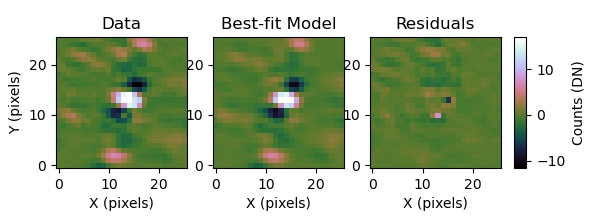
Appendix A KLIP Forward Model of the Data

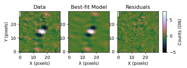
We compute a forward model of the PSF-subtracted image according to Pueyo (2016) to account for over- and self-subtraction effects. ADI imaging is particularly susceptible to self-subtraction effects, especially when there is little angular diversity, such as our data, which contains only two roll angles separated at $\sim 8$ degrees. Modeling these effects is essential for appropriately estimating the properties of the signal (flux, position). Figure 18 displays the comparison between the forward model and the PSF-subtracted image corresponding to the images displayed in Figure 3.

Figure 18: The KLIP forward model that accounts for over subtraction effects compared to the PSF-subtracted data in each of size filters.

Appendix B Keplerian Orbit Fit to HD 19467 Radial Velocities

We fit a Keplerian Orbit model to radial velocities of HD 19467 from HIRES and HARPS instruments, the latter published in Trifonov et al. (2020), catalog JA+A636A74rvbank table entries DRVmlcnzp and e_DRVmlcnzp. HIRES radial velocities, along with the new measurements are presented in Table 8. Using RadVel (Fulton et al., 2018), we determine that a model with a curvature term is slightly favored over a model without curvature, however the trend-only and trend plus curvature models are nearly indistinguishable (Table 9), based on $\Delta BIC$ and $\Delta AIC$ metrics. This is the first tentative evidence of curvature measured for HD 19467. Future follow up is needed to further support this finding.

Table 8: HIRES Radial Velocity Observations

Instrument	BJDTDB	RV	RV Error
HIRES	2450366.019	20.64	1.47
HIRES	2450418.943	29.50	2.17
HIRES	2450461.84	34.01	1.30
HIRES	2450715.103	26.13	4.20
HIRES	2450716.111	25.36	4.31
HIRES	2450786.847	23.29	2.38
HIRES	2450786.86	27.42	1.51
HIRES	2450806.904	22.50	1.50
HIRES	2450837.744	14.19	1.41
HIRES	2450839.743	19.41	1.49
HIRES	2451012.119	27.88	1.40
HIRES	2451013.12	19.74	1.31
HIRES	2451070.116	20.60	4.26
HIRES	2451072.984	29.72	4.36
HIRES	2451171.777	26.06	1.48
HIRES	2451410.128	21.00	1.51
HIRES	2451543.847	18.48	1.60
HIRES	2451551.792	19.77	1.47
HIRES	2451552.844	14.65	1.73
HIRES	2451582.73	24.84	1.70
HIRES	2451882.806	29.84	1.62
HIRES	2451900.783	23.36	1.48
HIRES	2452134.08	20.03	1.58
HIRES	2452242.908	19.50	1.42
HIRES	2452516.022	18.34	1.62
HIRES	2452575.902	10.04	1.72
HIRES	2452835.128	19.96	1.84
HIRES	2452926.089	19.92	4.43
HIRES	2453240.043	11.43	1.16
HIRES	2453427.785	8.38	1.20
HIRES	2453984.039	5.01	1.08
HIRES	2455807.035	-3.65	1.23
HIRES	2455808.105	-0.48	1.42
HIRES	2455809.088	1.84	1.22
HIRES	2455903.779	8.54	1.33
HIRES	2456152.11	-2.44	1.18
HIRES	2456210.015	1.14	1.49
HIRES	2456519.085	-0.97	1.28
HIRES	2456530.025	-7.90	1.20
HIRES	2456548.035	-0.47	1.33
HIRES	2456586.036	-2.87	1.41
HIRES	2456587.965	-3.16	1.42
HIRES	2456588.997	4.29	1.41
HIRES	2456613.908	-2.82	1.38
HIRES	2456637.791	-0.19	1.45
New data
HIRES	2457245.143	-0.38	1.18
HIRES	2458367.035	-15.44	1.76
HIRES	2459632.706	-10.11	1.51
HIRES	2459649.719	-13.26	1.48
HIRES	2459780.128	-14.46	1.29
HIRES	2459786.103	-4.38	1.16
HIRES	2459787.129	-15.52	1.20

Table 9: Model Comparison

AICc Qualitative Comparison	Free Parameters	$N_{\rm free}$	$N_{\rm data}$	RMS	$\ln{\mathcal{L}}$	BIC	AICc	$\Delta$AICc
AICc Favored Model	$\dot{\gamma}$, $\ddot{\gamma}$, $\sigma$, $\gamma$	8	128	3.40	-330.13	695.02	673.41	0.00
Nearly Indistinguishable	$\dot{\gamma}$, $\sigma$, $\gamma$	7	128	3.40	-332.43	692.91	673.88	0.47
Ruled Out	$\sigma$, $\gamma$	6	128	9.50	-426.33	872.85	856.43	183.02

Appendix C The MCMC posterior distribution for spectral fitting

Figure 19 shows the MCMC posterior distribution of the spectral fitting. The spatial structure seen in the posterior distribution reflects the step size of temperature (10 K), gravity (0.025 dex), and $\log(K_{\rm zz})$ (0.167) in the interpolated model grid. The sharp boundaries of radius at 0.5 $\rm R_{Jup}$ is reflects the lowest limit of radius range (0.5-1.5 $\rm{R_{Jup}}$) in the model fitting.

Figure 19: The posterior distribution of the MCMC fitting of Cholla models to the SPHERE-IRDIS spectra, SPHERE K12 photometry, and the JWST NIRCam photometries.

References

- Aguirre Børsen-Koch et al. (2022) Aguirre Børsen-Koch, V., Rørsted, J. L., Justesen, A. B., et al. 2022, MNRAS, 509, 4344, doi: 10.1093/mnras/stab2911
- Amara & Quanz (2012) Amara, A., & Quanz, S. P. 2012, MNRAS, 427, 948, doi: 10.1111/j.1365-2966.2012.21918.x
- Baraffe et al. (2003) Baraffe, I., Chabrier, G., Barman, T. S., Allard, F., & Hauschildt, P. H. 2003, A&A, 402, 701, doi: 10.1051/0004-6361:20030252
- Barman et al. (2011) Barman, T. S., Macintosh, B., Konopacky, Q. M., & Marois, C. 2011, ApJ, 733, 65, doi: 10.1088/0004-637X/733/1/65
- Bedding (2014) Bedding, T. R. 2014, in Asteroseismology, ed. P. L. Pallé & C. Esteban, 60
- Beichman et al. (2010) Beichman, C. A., Krist, J., Trauger, J. T., et al. 2010, PASP, 122, 162, doi: 10.1086/651057
- Bohlin et al. (2017) Bohlin, R. C., Mészáros, S., Fleming, S. W., et al. 2017, AJ, 153, 234, doi: 10.3847/1538-3881/aa6ba9
- Bowler et al. (2020) Bowler, B. P., Blunt, S. C., & Nielsen, E. L. 2020, AJ, 159, 63, doi: 10.3847/1538-3881/ab5b11
- Brandt et al. (2021a) Brandt, G. M., Dupuy, T. J., Li, Y., et al. 2021a, AJ, 162, 301, doi: 10.3847/1538-3881/ac273e
- Brandt (2021) Brandt, T. D. 2021, ApJS, 254, 42, doi: 10.3847/1538-4365/abf93c
- Brandt et al. (2021b) Brandt, T. D., Dupuy, T. J., Li, Y., et al. 2021b, AJ, 162, 186, doi: 10.3847/1538-3881/ac042e
- Brewer et al. (2016) Brewer, J. M., Fischer, D. A., Valenti, J. A., & Piskunov, N. 2016, ApJS, 225, 32, doi: 10.3847/0067-0049/225/2/32
- Brown et al. (1991) Brown, T. M., Gilliland, R. L., Noyes, R. W., & Ramsey, L. W. 1991, ApJ, 368, 599, doi: 10.1086/169725
- Burnham & Anderson (2002) Burnham, K. P., & Anderson, D. R., eds. 2002, Model Selection and Multimodel Inference: A Practical Information-Theoretic Approach (New York: Springer)
- Butler et al. (1996) Butler, R. P., Marcy, G. W., Williams, E., et al. 1996, PASP, 108, 500, doi: 10.1086/133755
- Butler et al. (2017) Butler, R. P., Vogt, S. S., Laughlin, G., et al. 2017, AJ, 153, 208, doi: 10.3847/1538-3881/aa66ca
- Carter et al. (2022) Carter, A. L., Hinkley, S., Kammerer, J., et al. 2022, arXiv e-prints, arXiv:2208.14990. https://arxiv.org/abs/2208.14990
- Casagrande et al. (2021) Casagrande, L., Lin, J., Rains, A. D., et al. 2021, MNRAS, 507, 2684, doi: 10.1093/mnras/stab2304
- Choi et al. (2016) Choi, J., Dotter, A., Conroy, C., et al. 2016, ApJ, 823, 102, doi: 10.3847/0004-637X/823/2/102
- Chontos et al. (2021) Chontos, A., Huber, D., Sayeed, M., & Yamsiri, P. 2021, arXiv e-prints, arXiv:2108.00582. https://arxiv.org/abs/2108.00582
- Corsaro et al. (2020) Corsaro, E., McKeever, J. M., & Kuszlewicz, J. S. 2020, A&A, 640, A130, doi: 10.1051/0004-6361/202037930
- Crepp et al. (2014) Crepp, J. R., Johnson, J. A., Howard, A. W., et al. 2014, ApJ, 781, 29, doi: 10.1088/0004-637X/781/1/29
- Crepp et al. (2015) Crepp, J. R., Rice, E. L., Veicht, A., et al. 2015, ApJ, 798, L43, doi: 10.1088/2041-8205/798/2/L43
- Cutri & et al. (2012) Cutri, R. M., & et al. 2012, VizieR Online Data Catalog, II/311
- Cutri et al. (2003) Cutri, R. M., Skrutskie, M. F., van Dyk, S., et al. 2003, VizieR Online Data Catalog, II/246
- Foreman-Mackey et al. (2017) Foreman-Mackey, D., Agol, E., Ambikasaran, S., & Angus, R. 2017, AJ, 154, 220, doi: 10.3847/1538-3881/aa9332
- Foreman-Mackey et al. (2013) Foreman-Mackey, D., Hogg, D. W., Lang, D., & Goodman, J. 2013, PASP, 125, 306, doi: 10.1086/670067
- Fouesneau (2022) Fouesneau, M. 2022, pyphot, 1.4.3. https://github.com/mfouesneau/pyphot
- Fulton et al. (2018) Fulton, B. J., Petigura, E. A., Blunt, S., & Sinukoff, E. 2018, PASP, 130, 044504, doi: 10.1088/1538-3873/aaaaa8
- García & Ballot (2019) García, R. A., & Ballot, J. 2019, Living Reviews in Solar Physics, 16, 4, doi: 10.1007/s41116-019-0020-1
- Girard et al. (2022) Girard, J. H., Leisenring, J., Kammerer, J., et al. 2022, in Society of Photo-Optical Instrumentation Engineers (SPIE) Conference Series, Vol. 12180, Space Telescopes and Instrumentation 2022: Optical, Infrared, and Millimeter Wave, ed. L. E. Coyle, S. Matsuura, & M. D. Perrin, 121803Q, doi: 10.1117/12.2629636
- Gomes da Silva et al. (2021) Gomes da Silva, J., Santos, N. C., Adibekyan, V., et al. 2021, A&A, 646, A77, doi: 10.1051/0004-6361/202039765
- Harris et al. (2020) Harris, C. R., Millman, K. J., van der Walt, S. J., et al. 2020, Nature, 585, 357, doi: 10.1038/s41586-020-2649-2
- Huber et al. (2009) Huber, D., Stello, D., Bedding, T. R., et al. 2009, Communications in Asteroseismology, 160, 74. https://arxiv.org/abs/0910.2764
- Huber et al. (2013) Huber, D., Chaplin, W. J., Christensen-Dalsgaard, J., et al. 2013, ApJ, 767, 127, doi: 10.1088/0004-637X/767/2/127
- Huber et al. (2017) Huber, D., Zinn, J., Bojsen-Hansen, M., et al. 2017, ApJ, 844, 102, doi: 10.3847/1538-4357/aa75ca
- Huber et al. (2022) Huber, D., White, T. R., Metcalfe, T. S., et al. 2022, AJ, 163, 79, doi: 10.3847/1538-3881/ac3000
- Hunter (2007) Hunter, J. D. 2007, Computing in Science & Engineering, 9, 90, doi: 10.1109/MCSE.2007.55
- Jakobsen et al. (2022) Jakobsen, P., Ferruit, P., Alves de Oliveira, C., et al. 2022, A&A, 661, A80, doi: 10.1051/0004-6361/202142663
- Jenkins et al. (2016) Jenkins, J. M., Twicken, J. D., McCauliff, S., et al. 2016, in Society of Photo-Optical Instrumentation Engineers (SPIE) Conference Series, Vol. 9913, Software and Cyberinfrastructure for Astronomy IV, ed. G. Chiozzi & J. C. Guzman, 99133E, doi: 10.1117/12.2233418
- Karalidi et al. (2021) Karalidi, T., Marley, M., Fortney, J. J., et al. 2021, ApJ, 923, 269, doi: 10.3847/1538-4357/ac3140
- Krist et al. (1997) Krist, J. E., Burrows, C. J., Stapelfeldt, K. R., et al. 1997, ApJ, 481, 447, doi: 10.1086/304056
- Krist et al. (2007) Krist, J. E., Beichman, C. A., Trauger, J. T., et al. 2007, in Society of Photo-Optical Instrumentation Engineers (SPIE) Conference Series, Vol. 6693, Techniques and Instrumentation for Detection of Exoplanets III, ed. D. R. Coulter, 66930H, doi: 10.1117/12.734873
- Lafrenière et al. (2007) Lafrenière, D., Marois, C., Doyon, R., Nadeau, D., & Artigau, É. 2007, ApJ, 660, 770, doi: 10.1086/513180
- Lavie et al. (2017) Lavie, B., Mendonça, J. M., Mordasini, C., et al. 2017, AJ, 154, 91, doi: 10.3847/1538-3881/aa7ed8
- Lim & Hanley (2016) Lim, P. L., & Hanley, C. 2016, synphot, Zenodo, doi: 10.5281/zenodo.3673988
- Linder et al. (2019) Linder, E. F., Mordasini, C., Mollière, P., et al. 2019, A&A, 623, A85, doi: 10.1051/0004-6361/201833873
- Lodders (2010) Lodders, K. 2010, in Formation and Evolution of Exoplanets, 157, doi: 10.1002/9783527629763.ch8
- Lorenzo-Oliveira et al. (2018) Lorenzo-Oliveira, D., Freitas, F. C., Meléndez, J., et al. 2018, A&A, 619, A73, doi: 10.1051/0004-6361/201629294
- Maire et al. (2020) Maire, A. L., Molaverdikhani, K., Desidera, S., et al. 2020, A&A, 639, A47, doi: 10.1051/0004-6361/202037984
- Manjavacas et al. (2019) Manjavacas, E., Apai, D., Lew, B. W. P., et al. 2019, ApJ, 875, L15, doi: 10.3847/2041-8213/ab13b9
- Marley et al. (2012) Marley, M. S., Saumon, D., Cushing, M., et al. 2012, ApJ, 754, 135, doi: 10.1088/0004-637X/754/2/135
- Marley et al. (2021) Marley, M. S., Saumon, D., Visscher, C., et al. 2021, ApJ, 920, 85, doi: 10.3847/1538-4357/ac141d
- Mathur et al. (2012) Mathur, S., Metcalfe, T. S., Woitaszek, M., et al. 2012, ApJ, 749, 152, doi: 10.1088/0004-637X/749/2/152
- Mawet et al. (2014) Mawet, D., Milli, J., Wahhaj, Z., et al. 2014, ApJ, 792, 97, doi: 10.1088/0004-637X/792/2/97
- McQuillan et al. (2014) McQuillan, A., Mazeh, T., & Aigrain, S. 2014, ApJS, 211, 24, doi: 10.1088/0067-0049/211/2/24
- Mesa et al. (2020) Mesa, D., D’Orazi, V., Vigan, A., et al. 2020, MNRAS, 495, 4279, doi: 10.1093/mnras/staa1444
- Metcalfe et al. (2014) Metcalfe, T. S., Creevey, O. L., Doğan, G., et al. 2014, ApJS, 214, 27, doi: 10.1088/0067-0049/214/2/27
- Mukherjee et al. (2022) Mukherjee, S., Batalha, N. E., Fortney, J. J., & Marley, M. S. 2022, arXiv e-prints, arXiv:2208.07836. https://arxiv.org/abs/2208.07836
- Nakajima et al. (1995) Nakajima, T., Oppenheimer, B. R., Kulkarni, S. R., et al. 1995, Nature, 378, 463, doi: 10.1038/378463a0
- Nissen et al. (2020) Nissen, P. E., Christensen-Dalsgaard, J., Mosumgaard, J. R., et al. 2020, A&A, 640, A81, doi: 10.1051/0004-6361/202038300
- Perrin et al. (2014) Perrin, M. D., Sivaramakrishnan, A., Lajoie, C.-P., et al. 2014, in Society of Photo-Optical Instrumentation Engineers (SPIE) Conference Series, Vol. 9143, Space Telescopes and Instrumentation 2014: Optical, Infrared, and Millimeter Wave, ed. J. Oschmann, Jacobus M., M. Clampin, G. G. Fazio, & H. A. MacEwen, 91433X, doi: 10.1117/12.2056689
- Pietrinferni et al. (2004) Pietrinferni, A., Cassisi, S., Salaris, M., & Castelli, F. 2004, ApJ, 612, 168, doi: 10.1086/422498
- Pueyo (2016) Pueyo, L. 2016, ApJ, 824, 117, doi: 10.3847/0004-637X/824/2/117
- Ricker et al. (2015) Ricker, G. R., Winn, J. N., Vanderspek, R., et al. 2015, Journal of Astronomical Telescopes, Instruments, and Systems, 1, 014003, doi: 10.1117/1.JATIS.1.1.014003
- Rieke et al. (in press) Rieke, M. J., Kelly, D. M., Misselt, K., et al. in press, PASP, arXiv:2212.12069. https://arxiv.org/abs/2212.12069
- Rosenthal et al. (2021) Rosenthal, L. J., Fulton, B. J., Hirsch, L. A., et al. 2021, ApJS, 255, 8, doi: 10.3847/1538-4365/abe23c
- Santos et al. (2021) Santos, A. R. G., Breton, S. N., Mathur, S., & García, R. A. 2021, ApJS, 255, 17, doi: 10.3847/1538-4365/ac033f
- Silva Aguirre et al. (2017) Silva Aguirre, V., Lund, M. N., Antia, H. M., et al. 2017, ApJ, 835, 173, doi: 10.3847/1538-4357/835/2/173
- Smith et al. (2012) Smith, J. C., Stumpe, M. C., Van Cleve, J. E., et al. 2012, PASP, 124, 1000, doi: 10.1086/667697
- Soummer et al. (2012) Soummer, R., Pueyo, L., & Larkin, J. 2012, ApJ, 755, L28, doi: 10.1088/2041-8205/755/2/L28
- STScI Development Team (2013) STScI Development Team. 2013, pysynphot: Synthetic photometry software package, Astrophysics Source Code Library, record ascl:1303.023. http://ascl.net/1303.023
- Stumpe et al. (2012) Stumpe, M. C., Smith, J. C., Van Cleve, J. E., et al. 2012, PASP, 124, 985, doi: 10.1086/667698
- Tayar et al. (2022) Tayar, J., Claytor, Z. R., Huber, D., & van Saders, J. 2022, ApJ, 927, 31, doi: 10.3847/1538-4357/ac4bbc
- Trifonov et al. (2020) Trifonov, T., Tal-Or, L., Zechmeister, M., et al. 2020, A&A, 636, A74, doi: 10.1051/0004-6361/201936686
- Ulrich (1986) Ulrich, R. K. 1986, ApJ, 306, L37, doi: 10.1086/184700
- Virtanen et al. (2020) Virtanen, P., Gommers, R., Oliphant, T. E., et al. 2020, Nature Methods, 17, 261, doi: 10.1038/s41592-019-0686-2
- Vousden et al. (2016) Vousden, W. D., Farr, W. M., & Mandel, I. 2016, MNRAS, 455, 1919, doi: 10.1093/mnras/stv2422
- Wang et al. (2015) Wang, J. J., Ruffio, J.-B., De Rosa, R. J., et al. 2015, pyKLIP: PSF Subtraction for Exoplanets and Disks, Astrophysics Source Code Library, record ascl:1506.001. http://ascl.net/1506.001
- Wood et al. (2019) Wood, C. M., Boyajian, T., von Braun, K., et al. 2019, ApJ, 873, 83, doi: 10.3847/1538-4357/aafe01