1 Introduction
Graph Convolutional Networks (GCNs) (Kipf & Welling, 2017; Hammond et al., 2011; Defferrard et al., 2016) generalize Euclidean convolutional networks to the graph setting by
replacing convolutional filters by functional calculus filters; i.e. scalar functions applied to a suitably chosen graph-shift-oprator capturing the geometry of the underlying graph.
A key concept in trying to
understand the underlying reasons for the superior numerical performance of such networks on graph learning tasks
(as well as a guiding principle for the design of new architectures) is the concept of stability. In the Euclidean setting,
investigating stability essentially amounts to exploring the variation of the output of a network under non-trivial changes of its input (Mallat, 2012; Wiatowski & Bölcskei, 2018).
In the graph-setting, additional complications are introduced: Not only input signals, but now also the graph shift operators facilitating the convolutions on the graphs may vary. Even worse, there might also occur changes in the topology or vertex sets of the investigated graphs – e.g. when two dissimilar graphs describe the same underlying phenomenon – under which graph convolutional networks should also remain stable. This last stability property is often also referred to as transferability
(Levie et al., 2019a).
works investigated stability under changes in graph-shift operators for specific filters (Levie et al., 2019b; Gama et al., 2020) or the effect of graph-rewiring when choosing a specific graph shift operator (Kenlay et al., 2021). Stability to topological perturbations has been established for (large) graphs discretising the same underlying topological space (Levie et al., 2019a), the same graphon (Ruiz et al., 2020; Maskey et al., 2021) or for graphs drawn from the same statistical distribution (Keriven et al., 2020; Gao et al., 2021).
Common among all these previous works are two themes limiting practical applicability:
First and foremost,
the class of filters to which results are applicable is often severely restricted. The same is true for the class of considered graph shift operators; with non-normal operators (describing directed graphs) either explicitly or implicitly excluded. Furthermore – when investigating transferability properties – results are almost exclusively available under the assumption that graphs are large and either discretize the same underlying ’continuous’ limit object suffieciently well, or are drawn from the same statistical distributions. While these are of course relevant regimes, they do not allow to draw conclusions beyond such asymptotic settings, and are for example unable to deal with certain spatial graphs, inapplicable to small-to-medium sized social networks and incapable of capturing the inherent multi-scale nature of molecular graphs (as further discussed below).
Finally, hardly any work has been done on relating the stability to input-signal perturbations to network properties such as the interplay of utilized filters or employed non-linearities.
The main focus of this work is to provide alleviation in this situation and develop a ’general theory of stability’ for GCNs – agnostic to the types of utilized filters, graph shift operators and non-linearities; with practically relevant transferability guarantees not contingent on potentially underlying limit objects. To this end, Section 2 recapitulates the
fundamentals of
GCNs in a language adapted to our endeavour. Sections 3 and 4 discuss stability to node- and edge-level perturbations. Section 5 discusses stability to structural perturbations. Section 6 discusses feature aggregation and
Section 7 provides numerical evidence.
4 Stability to Edge Perturbations
Operators capturing graph-geometries might only be known approximately in real world tasks; e.g. if edge weights are only known to a certain level of precision.
Hence it is important that graph convolutional networks be insensitive to small changes in the characteristic operators . Since we consider graphs with arbitrary vertex weights , we also have to consider the possibility that these weights are only known to a certain level of precision.
In this case, not only do the characteristic operators , differ, but also the the spaces , on which they act. To capture this setting mathematically, we assume in this section that there is a linear operator facilitating contact between signal spaces (of not-necessarily the same dimension). We then measure closeness of characteristic operators in the respective spaces by considering the generalized norm-difference ; with translating between the respective spaces.
Before investigating the stability of entire networks
we first comment on single-filter stability.
For normal operators
we then find the following result, proved in Appendix A building on ideas first developed in (Wihler, 2009).
Lemma 4.1.
Denote by the Frobenius norm and let and be normal on and respectively. Let be Lipschitz continuous with Lipschitz constant . For any linear we have
Unfortunately, scalar Lipschitz continuity only directly translates to operator functions if they are applied to normal operators and when using Frobenius norm (as opposed to e.g. spectral norm). For general operators we have the following somewhat weaker result, proved in Appendix F:
Lemma 4.2.
Let be operators on on , with .
Let be linear.
With for holomorphic and for entire, we have .
Each itself is interpretable as a semi-norm. For GCNs we find the following (c.f. Appendix F):
Theorem 4.3.
Let be the maps associated to -layer graph convolutional networks with the same non-linearities and filters, but based on different graph signal spaces , characteristic operators and connecting operators .
Assume as well as and for some and all .
Assume that there are identification operators () commuting with non-linearities and connecting operators in the sense of and .
Depending on whether normal or arbitrary characteristic operators are used, define or . Choose such that for all . Finally assume that and with if both operators are normal and otherwise. Then we have for all and with the operator that the copies of induce through concatenation that
.
The result persists with slightly altered constants, if identification operators only almost commute with non-linearities and/or connecting operators, as Appendix G further elucidates.
Since we estimated various constants ()
of the individual layers by global
ones,
the derived stability constant is clearly not
tight.
However it portrays requirements for stability to edge level perturbations well: While the
(spectral) interplay of Section 3 remains important, it is now especially large single-filter stability constants in the sense of Lemmata 4.1 and 4.2 that should be penalized during training.
Appendix C Complex Analysis
A general reference for topics discussed in this section is Bak & Newman (2017).
For a complex valued function of a single complex variable, the derivative of at a point in its domain of definition is defined as the limit
|
|
|
(39) |
For this limit to exist, it needs to be independent of the ’direction’ in which approaches , which is a stronger requirement than being real-differentiable. A function is called holomorphic on an open set if it is complex differentiable at every point in . It is called entire if it is complex differentiable at every point in . Every entire function has an everywhere convergent power series representation
|
|
|
(40) |
If a function is analytic (i.e. can be expanded into a power series), we have
|
|
|
(41) |
for any circle encircling by Cauchy’s integral formula.
In fact, the integration contour need not be a circle , but may be the boundary of any so called Cauchy domain containing :
Definition C.1.
A subset of the complex plane is called a Cauchy domain if is open, has a finite number of components (the closure of two of which are disjoint) and the boundary of of is composed of a finite number of closed rectifiable Jordan curves, no two of which intersect.
Equation (41) forms the backbone of complex analysis. Since the integral
|
|
|
(42) |
is well defined for holomorphic and any operator for which and are disjoint (c.f. e.g. Post (2012) for details), we can essentially take (42) as a defining equation through which one might apply holomorphic functions to operators.
While functions that are everywhere complex differentiable have a series representation according to (40), complex functions that are holomorphic only on have a series representation (called Laurent series) according to
|
|
|
(43) |
If these functions are assumed to be regular at infinity, no terms with positive exponent are permitted and (changing the indexing) we may thus write
|
|
|
(44) |
Motivated by this, we now prove the following consistency result:
Lemma C.2.
With the notation of Section 2 we have for any and that
|
|
|
(45) |
where we interpret the left hand side of the equation in terms of inversion and matrix powers.
Proof.
We first note that we may write
|
|
|
(46) |
for using standard results in matrix analysis (namely the ’Neumann Characterisation of the Resolvent’ which is obtained by repeated application of a resolvent identity; c.f. Post (2012) for more details).
We thus find
|
|
|
(47) |
Using the fact that
|
|
|
(48) |
then yields the claim.
∎
Appendix J Collapsing strong Edges: Proofs and further Details
We utilize the notation introduced in Section 5.2. Beyond this, we denote the positive semi-definite form induced by the energy functional by
|
|
|
(99) |
We further use the notation .
With
|
|
|
(100) |
Similar considerations apply when is replaced by .
Let us next solve the convex optimization program (10) introduced in Definition 5.5, restated here for convenience:
Definition J.1.
For each , define the signal as the unique solution to the convex optimization program
|
|
|
(101) |
As a first step we note that all entries of are real and non-negative, which follows since each summand in (100) is non-increasing under the map due to the reverse triangle .
To find the explicit form of , fix and denote by the signal defined by setting it to for and with a set of free parameters in . We then have
|
|
|
|
(102) |
|
|
|
|
(103) |
By definition, depends smoothly on the parameters . Finding the minimizer of the convex optimization program (10) is then equivalent to finding the values at which we have
|
|
|
(104) |
We note
|
|
|
(105) |
Collecting these equations for all parameters into a matrix equation, we find that the ’Greek entries’ of the vector are given explicitly by
|
|
|
(106) |
with degrees in denoted by . Let us denote the restriction of to Greek entries, thought of as a vector in by .
Given the degree corresponding to a Greek index, we decompose it as
|
|
|
(107) |
with accounting for edges from to other greek vertices
|
|
|
(108) |
and accounting for edges from to Latin vertices
|
|
|
(109) |
Recall that we also may write
|
|
|
(110) |
We may then write
|
|
|
|
(111) |
|
|
|
|
(112) |
where we made the obvious definitions for the matrices and and denoted by the vector with entries .
Let us also use the notation
|
|
|
(113) |
Next we want to establish that is invertible.
For this we first note that that is the graph Laplacian of the subgraph ; which we assume to be connected. Hence is positive semi-definite with the eigenspace corresponding to the eigenvalue zero being spanned by (entry-wise) constant vectors. Since all entries of are non-negative, the operator is also positive semi-definite. Since we assume that the vertex is connected to at least one other vertex in , there is at least one entry in that is strictly greater than zero. We show that this already implies that is in fact also positive definite and hence invertible. Indeed, for any we have
|
|
|
(114) |
Both terms on the right hand side are non-negative. If is a constant (non-zero) vector, the first term vanishes, but since at least one entry of is strictly positive, with all others being non-negative, the second term on the right hand side is strictly positive. If is non-constant, the first term on the right hand side is larger than zero. Hence is positive definite and thus invertible. Similarly one proves that (for any ) the operator is positive definite and hence invertible. Thus we now know that the operator
|
|
|
(115) |
utilized in (106) is indeed invertible.
We note (again with the restriction of to Greek entries thought of as a vector in denoted by ) that we may equivalently write (106) as
|
|
|
(116) |
and
|
|
|
(117) |
thought of as an element of . To proceed, we now first focus on the case , for which we may write (116) equivalently as
|
|
|
(118) |
Since is independent of , we may take the limit and arrive at
|
|
|
(119) |
which is uniquely solved by .
Since we assume , we can now investigate the solution for non-zero through perturbation theory. We write
|
|
|
(120) |
with and find from (118) – using – the defining equation
|
|
|
(121) |
From this we obtain the estimate
|
|
|
(122) |
where we denote by the space graph signal space equipped with node weights .
We note that both and are positive semi-definite and we thus obtain
|
|
|
(123) |
for the minimal eigenvalues of the respective operators. Hence
|
|
|
(124) |
and thus also
|
|
|
(125) |
Since we may write
|
|
|
(126) |
From (116) we know that for we have .
We now also want to bound in terms of . We will do this by establishing the relationship
|
|
|
(127) |
and then utilizing our estimate on established above. To prove (127), we will need the concept of harmonic extensions:
Definition J.2.
Denote by the graph signal space equipped with the node weights . Given an arbitrary signal a harmonic extension of to all of is a signal satisfying
|
|
|
(128) |
We first note that the concept of harmonic extensions is both well-defined an well-behaved:
Lemma J.3.
Fix . There exists a unique harmonic extension of .
It is given as the solution to the convex optimization program
|
|
|
(129) |
Furthermore if and are the harmonic extensions of and , then is the (unique) harmonic extension of .
Proof.
We write a signal as with and . We then notice
|
|
|
|
(130) |
|
|
|
|
(131) |
|
|
|
|
(132) |
|
|
|
|
(133) |
Here, we treated and its complex conjugate as independent variables and used that is a real-valued functional for the first equivalence. As harmonic extensions are thus equivalently characterised as the solutions of convex minimization programs, they are unique.
To prove the last statement, we note that by linearity of the graph Laplacian, certainly is a harmonic extension of . Since harmonic extensions are unique, it is the only one.
∎
After this preparatory effort, we are now ready to prove (127):
Lemma J.4.
For any the signals form a partition of unity of :
|
|
|
(134) |
Equivalently we have
|
|
|
(135) |
As an immediate Corollary we obtain
Corollary J.5.
For any the signals form a partition of unity of :
|
|
|
(136) |
Proof.
Using the ’boundary conditions’ in (10), it is straightforward to verify that (134) is equivalent to (136). From Lemma J.3 we now know that , originally characterised as the solution of the problem
|
|
|
(137) |
is equivalently characterised as the harmonic extension of .
From the last statement of Lemma J.3, we know that is the unique harmonic extension of
|
|
|
(138) |
But this – in turn – is the unique solution of the problem
|
|
|
(139) |
Since we have
|
|
|
(140) |
which is the lowest possible attainable value of , and setting is compatible with the ’boundary condition’ , we know that is the (unique) harmonic extension of . By the last statement of Lemma J.3 we thus have
|
|
|
(141) |
Having established that we may write
|
|
|
(142) |
together with the fact that every entry of each is non-negative, we now know that
|
|
|
(143) |
Furthermore – using our earlier estimate (125) – we now easily obtain
|
|
|
(144) |
Hence – by positivity of the entries – we also have for each individual that
|
|
|
(145) |
For the weights we then find
|
|
|
(146) |
if . We also write . If , we have
|
|
|
(147) |
Having set the scene, we are now ready to prove Theorem 5.4. Following Post & Simmer (2017), instead of checking the conditions of Definition 5.1 and Definition 5.2 it is instead sufficient to check the following, with as defined in Section 5.2 to establish Theorem 5.6:
Lemma J.6.
In addition to identification operators , assume that there exist additional operators and so that the following set of equations is satisfied with
|
|
|
(148) |
|
|
|
(149) |
|
|
|
(150) |
|
|
|
(151) |
Then the (normal) operators and are (doubly) (-1)-
()
-close with identification-operator .
Here, we always have and )
Proof.
This follows immediately after combining Proposition with Theorem of Post (2012).
∎
We set and and now determine the individual values for which these equations are satisfied:
Left-hand-side of (148):
For the left hand side of (148) we note (using and the fact that the form a partition of unity):
|
|
|
|
(152) |
|
|
|
|
(153) |
|
|
|
|
(154) |
|
|
|
|
(155) |
|
|
|
|
(156) |
Here the second to last inequality follows from the definition of the weights . Thus the left hand side of (148) holds with
|
|
|
(157) |
Right-hand-side of (148):
The right hand side of (148) holds trivially with
|
|
|
(158) |
since we have chosen .
Left-hand-side of (149):
Now let us check the l.h.s. of (149). We have:
|
|
|
(159) |
Using the constant defined in (126) we have
|
|
|
(160) |
if . We also write . If , we have
|
|
|
(161) |
We next note
|
|
|
(162) |
with the vector with entries .
Thus for we find
|
|
|
(163) |
We thus find
|
|
|
|
(164) |
|
|
|
|
(165) |
|
|
|
|
(166) |
|
|
|
|
(167) |
To bound the first term of the estimate, we note (for ) and small enough:
|
|
|
(169) |
We also note (for )
|
|
|
|
(170) |
Thus we find
|
|
|
(171) |
To estimate the second term, we estimate
|
|
|
|
(172) |
to obtain
|
|
|
|
(173) |
|
|
|
|
(174) |
|
|
|
|
(175) |
Thus we find (using that is a non-negative number and we have )
|
|
|
|
(176) |
|
|
|
|
(177) |
|
|
|
|
(178) |
|
|
|
|
(179) |
|
|
|
|
(180) |
|
|
|
|
(181) |
Let us thus turn to the remaining term; corresponding to : We have
|
|
|
|
(183) |
We first deal with the left summand. We note
|
|
|
|
(184) |
|
|
|
|
(185) |
|
|
|
|
(186) |
|
|
|
|
(187) |
|
|
|
|
(188) |
|
|
|
|
(189) |
|
|
|
|
(190) |
|
|
|
|
(191) |
Thus, under the assumption (implying ), we have
|
|
|
(193) |
This implies that we have
|
|
|
(194) |
For the right-hand-side summand of the estimate in (183) we note
|
|
|
|
(195) |
|
|
|
|
(196) |
|
|
|
|
(197) |
|
|
|
|
(198) |
|
|
|
|
(199) |
Putting it all together, we find for that
|
|
|
(201) |
with
|
|
|
(202) |
Thus the left hand side of (149) holds with
|
|
|
(203) |
Right-hand-side of (149):
Hence let us now check the right hand side of (149). We note
|
|
|
(204) |
Let us denote by the matrix representation
|
|
|
(205) |
We use the triangle inequality to arrive at
|
|
|
(206) |
Using the fact that for we have an
we find in the ()-limit that
|
|
|
(207) |
with
|
|
|
(208) |
acting on . For any element , let us denote its restriction to by .
We thus find
|
|
|
|
(209) |
|
|
|
|
(210) |
|
|
|
|
(211) |
|
|
|
|
(212) |
|
|
|
|
(213) |
|
|
|
|
(214) |
|
|
|
|
(215) |
To proceed, we prove the following Lemma:
Lemma J.7.
Let . Denote by the minimum number of edges for which needed to connect and by a path. Set
|
|
|
(216) |
Furthermore set
|
|
|
(217) |
We have
|
|
|
(218) |
We call the connectivity constant of the sub-graph and note that it is well-defined since we assume to be connected.
Proof.
Fix and . Let be the vertices traversed by a path of minimal length determining . We then have
|
|
|
|
(219) |
|
|
|
|
(220) |
|
|
|
|
(221) |
|
|
|
|
(222) |
|
|
|
|
(223) |
|
|
|
|
(224) |
∎
With the help of this Lemma we then find
|
|
|
|
(225) |
|
|
|
|
(226) |
To derive a bound for in the second term of the estimate (206), we write
|
|
|
(227) |
Here we denote by
|
|
|
(228) |
the adjoint of the operator
|
|
|
(229) |
Clearly so that we have
|
|
|
(230) |
To bound we note that is diagonal and we have
|
|
|
(231) |
so that
|
|
|
|
(232) |
|
|
|
|
(233) |
|
|
|
|
(234) |
|
|
|
|
(235) |
|
|
|
|
(236) |
|
|
|
|
(237) |
To estimate we note
|
|
|
(238) |
We can consider the map
|
|
|
(239) |
as a composition of maps
|
|
|
(240) |
For the map we find . Similarly we find for the map that .
To bound the operator norm of the map , we use that the operator-norm is smaller than the maximal column-sum times .
Hence for as a map from to we find
|
|
|
|
(241) |
|
|
|
|
(242) |
|
|
|
|
(243) |
|
|
|
|
(244) |
Here we estimated
|
|
|
(245) |
In total, we find for the operator-norm of
|
|
|
(246) |
that
|
|
|
(247) |
Thus let us now investigate . As before. let us denote by the restriction of an element to . We have
|
|
|
|
(248) |
|
|
|
|
(249) |
|
|
|
|
(250) |
|
|
|
|
(251) |
We note for the matrix representation of the first term, that (with ) we have
|
|
|
(252) |
Using the ’maximal row sum trick’ complementary to the ’maximal column sum trick’ already used for above and recalling the definition of the weights
|
|
|
(253) |
we find
|
|
|
(254) |
|
|
|
(255) |
|
|
|
(256) |
|
|
|
(257) |
|
|
|
(258) |
|
|
|
(259) |
|
|
|
(260) |
It remains to bound the second term. We find (using ):
|
|
|
|
(261) |
|
|
|
|
(262) |
|
|
|
|
(263) |
|
|
|
|
(264) |
|
|
|
|
(265) |
|
|
|
|
(266) |
|
|
|
|
(267) |
|
|
|
|
(268) |
|
|
|
|
(269) |
Thus we find
|
|
|
(270) |
In total, using (206) and (230), we find
|
|
|
|
(271) |
|
|
|
|
(272) |
|
|
|
|
(273) |
|
|
|
|
(274) |
and may hence set
|
|
|
|
(275) |
|
|
|
|
(276) |
|
|
|
|
(277) |
Left-hand-side of (150):
The left hand side of (150) is true with by definition.
Right-hand-side of (150):
Let us thus check the right hand side of (150):
We have
|
|
|
(278) |
We note
|
|
|
|
(279) |
We first deal with the left hand term of the estimate and note that for we have
|
|
|
(280) |
and
in the limit that
|
|
|
|
(281) |
|
|
|
|
(282) |
|
|
|
|
(283) |
|
|
|
|
(284) |
|
|
|
|
(285) |
Here we applied Lemma J.7. Comparing the and terms, we find
|
|
|
|
(287) |
|
|
|
|
(288) |
|
|
|
|
(289) |
|
|
|
|
(290) |
|
|
|
|
(291) |
Thus we have
|
|
|
|
(292) |
|
|
|
|
(293) |
For the remaining term in (279) we note
|
|
|
|
(294) |
|
|
|
|
(295) |
|
|
|
|
(296) |
|
|
|
|
(297) |
|
|
|
|
(298) |
|
|
|
|
(299) |
Equation (151):
It finally only remains to prove the energy differences of (151) and establish
|
|
|
(301) |
We note that the (unique) operator associated to the energy via
|
|
|
(302) |
is given by
|
|
|
(303) |
Here the notation "" signifies that nodes and are connected within through edges with positive edge-weights .
Similarly the operator associated to via
|
|
|
(304) |
is given by
|
|
|
(305) |
with the equivalence relation precisely signifying that .
As before. let us denote by the restriction of an element to .
We note
|
|
|
(306) |
on the smaller graph .
For the graph we find
|
|
|
|
(307) |
|
|
|
|
(308) |
Remembering that we have
|
|
|
(309) |
we note
|
|
|
|
(310) |
|
|
|
|
(311) |
Let us first bound the terms corresponding to :
We have
|
|
|
|
(312) |
|
|
|
|
(313) |
as well as
|
|
|
|
(314) |
|
|
|
|
(315) |
|
|
|
|
(316) |
|
|
|
|
(317) |
|
|
|
|
(318) |
Hence (for )
|
|
|
(319) |
For we find – using Lemma J.7 – that
|
|
|
(320) |
and hence
|
|
|
(321) |
To bound we note
|
|
|
|
(322) |
|
|
|
|
(323) |
|
|
|
|
(324) |
Thus we find – using Cauchy-Schwarz – that
|
|
|
|
(325) |
|
|
|
|
(326) |
|
|
|
|
(327) |
|
|
|
|
(328) |
|
|
|
|
(329) |
Here we denoted by the degree of the node .
We further note
|
|
|
(331) |
Writing
|
|
|
(332) |
for the sum of ’internal’ degrees of greek nodes within at and
|
|
|
(333) |
for the ’total connection strength’ between the Greek and Latin sector, we thus find
|
|
|
(334) |
It remains to bound the term in (319).
To this end we note
|
|
|
(335) |
and
|
|
|
|
(336) |
|
|
|
|
(337) |
For the difference of the energy forms we thus find
|
|
|
|
(338) |
|
|
|
|
(339) |
|
|
|
|
(340) |
|
|
|
|
(341) |
|
|
|
|
(342) |
We have
|
|
|
|
(343) |
|
|
|
|
(344) |
with the last term vanishing by symmetry. This implies
|
|
|
|
(345) |
|
|
|
|
(346) |
|
|
|
|
(347) |
|
|
|
|
(348) |
|
|
|
|
(349) |
|
|
|
|
(350) |
|
|
|
|
(351) |
|
|
|
|
(352) |
|
|
|
|
(353) |
|
|
|
|
(354) |
|
|
|
|
(355) |
Continuing, we find
|
|
|
|
(357) |
|
|
|
|
(358) |
|
|
|
|
(359) |
|
|
|
|
(360) |
|
|
|
|
(361) |
|
|
|
|
(362) |
This – in turn – we can write as
|
|
|
|
(363) |
with
|
|
|
(364) |
and
|
|
|
(365) |
For the first term, we find
|
|
|
|
(366) |
|
|
|
|
(367) |
For the second term we note
|
|
|
|
(368) |
|
|
|
|
(369) |
|
|
|
|
(370) |
![[Uncaptioned image]](/html/2301.11443/assets/contour.png) Figure 1: Set-Visualisations
of the boundary is the usual positive orientation on (such that ’is on the left’ of ; cf. Fig. 1). Using elementary facts from complex analysis it can be shown that the resulting operator in (1) is independent of the specific choice of (Gindler, 1966).
While we will present results below in terms of this general definition – remaining agnostic to numerical implementation methods for the most part – it is instructive to consider a specific exemplary setting with definite and simple numerical implementation of such filters: To this end, chose an arbitrary point and set in the definitions above. Any function that is holomorphic on and regular at may then be represented by its Laurent series, which is of the form (Bak & Newman, 2017). For any with (i.e. ) evaluating the integral in (1) yields (c.f. Appendix C):
Figure 1: Set-Visualisations
of the boundary is the usual positive orientation on (such that ’is on the left’ of ; cf. Fig. 1). Using elementary facts from complex analysis it can be shown that the resulting operator in (1) is independent of the specific choice of (Gindler, 1966).
While we will present results below in terms of this general definition – remaining agnostic to numerical implementation methods for the most part – it is instructive to consider a specific exemplary setting with definite and simple numerical implementation of such filters: To this end, chose an arbitrary point and set in the definitions above. Any function that is holomorphic on and regular at may then be represented by its Laurent series, which is of the form (Bak & Newman, 2017). For any with (i.e. ) evaluating the integral in (1) yields (c.f. Appendix C):![[Uncaptioned image]](/html/2301.11443/assets/updaterule.png) Figure 2: Update Rule for a GCN
Let us denote the width of the network at layer by . The collection of hidden signals in this layer can then be thought of a single element of
(3)
Further let us write the collection of functional calculus filters utilized to generate the representation of this layer by . Further denoting the characteristic operator of this layer by , the update
rule (c.f. also Fig. 2) from the representation in to is then defined on each constituent in the direct sum as
Figure 2: Update Rule for a GCN
Let us denote the width of the network at layer by . The collection of hidden signals in this layer can then be thought of a single element of
(3)
Further let us write the collection of functional calculus filters utilized to generate the representation of this layer by . Further denoting the characteristic operator of this layer by , the update
rule (c.f. also Fig. 2) from the representation in to is then defined on each constituent in the direct sum as![[Uncaptioned image]](/html/2301.11443/assets/CollapsingGraphs.png) Figure 3: Collapsed (left) and original (right) Graphs
energy form on this signal space via .
Using this energy form, we now define a set comprised of signals, all of which live in . These signals are used to facilitate contact between the respective graph signal spaces and .
Figure 3: Collapsed (left) and original (right) Graphs
energy form on this signal space via .
Using this energy form, we now define a set comprised of signals, all of which live in . These signals are used to facilitate contact between the respective graph signal spaces and .![[Uncaptioned image]](/html/2301.11443/assets/Circles.png)
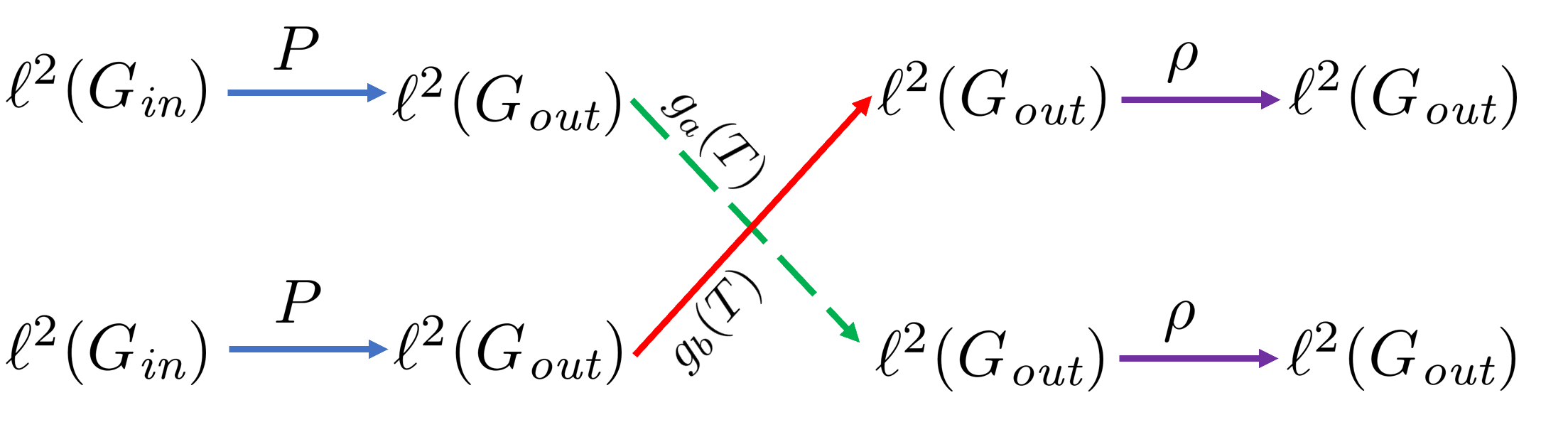
![[Uncaptioned image]](/html/2301.11443/assets/Aggregation.png) Figure 5: Graph Level Aggregation
this end, let be a target space of a GCN in the sense of (3). On each of the (in total ) summands of , we may apply the map . Stacking these maps, we build a map from to . Concatenating the map associated to an -layer GCN with this map
yields a map from to . We denote it by and find:
Figure 5: Graph Level Aggregation
this end, let be a target space of a GCN in the sense of (3). On each of the (in total ) summands of , we may apply the map . Stacking these maps, we build a map from to . Concatenating the map associated to an -layer GCN with this map
yields a map from to . We denote it by and find:
![[Uncaptioned image]](/html/2301.11443/assets/FusedFirstTwoExperimentshor.png)
![[Uncaptioned image]](/html/2301.11443/assets/SinRess.png)
![[Uncaptioned image]](/html/2301.11443/assets/NetTfup100.png)