Primordial black holes in loop quantum cosmology: The effect on the threshold
Abstract
Primordial black holes form in the early Universe and constitute one of the most viable candidates for dark matter. The study of their formation process requires the determination of a critical energy density perturbation threshold , which in general depends on the underlying gravity theory. Up to now, the majority of analytic and numerical techniques calculate within the framework of general relativity. In this work, using simple physical arguments we estimate semi-analytically the PBH formation threshold within the framework of quantum gravity, working for concreteness within loop quantum cosmology (LQC). In particular, for low mass PBHs formed close to the quantum bounce, we find a reduction in the value of up to compared to the general relativistic regime quantifying for the first time to the best of our knowledge how quantum effects can influence PBH formation within a quantum gravity framework. Finally, by varying the Barbero-Immirzi parameter of loop quantum gravity (LQG) we show its effect on the value of while using the observational/phenomenological signatures associated to ultra-light PBHs, namely the ones affected by LQG effects, we propose the PBH portal as a novel probe to constrain the potential quantum nature of gravity.
1 Introduction
PBHs, firstly proposed in the early ’70s [1, 2, 3], form in the early universe, typically during the Hot Big Bang (HBB) radiation-dominated (RD) era out of the gravitational collapse of enhanced cosmological perturbations. According to recent arguments, PBHs can naturally account for a part or the totality of dark matter [4, 5], seed the large-scale structures through Poisson fluctuations [6, 7, 8, 9] as well as the primordial magnetic fields through the presence of disks around them [10, 11]. At the same time, they are associated with a plethora of gravitational-wave (GW) signals from black-hole merging events [12, 13, 14, 15, 16] up to primordial scalar induced GWs [17, 18, 19, 20, 21, 22] (for a recent review see [23]). In particular, through the aforementioned GW portal, PBHs can act as well as a novel probe shedding light on the underlying gravity theory [24, 25]. Other hints in favor of PBHs can be found here [26].
In the standard PBH formation scenario, where PBHs form from the collapse of local overdensity regions, the PBH formation threshold depends in general on the shape of the energy density perturbation profile of the collapsing overdensity [27, 28, 29, 30, 31] as well as on the equation-of-state parameter at the time of PBH gravitational collapse [32, 33, 31, 34]. This critical threshold value is very important since it can affect significantly the abundance of PBHs, a quantity which is constrained by numerous observational probes [35].
From a historic perspective, after a first analytic calculation of by B. Carr and S. Hawking in 1975 [36, 32], was studied mostly through numerical hydrodynamic simulations by [37, 38, 39, 40, 41]. Within the last decade, there has been witnessed a remarkable progress regarding the determination both at the analytic as well as at the numerical level. In particular, at the analytic level, T.Harada, C-M. Yoo K. Kohri (HYK) in 2013 [33] refined the PBH formation threshold value obtained by Carr in 1975 by comparing the time at which the pressure sound wave crosses the overdensity collapsing to a PBH with the onset time of the gravitational collapse. Their expression for in the uniform Hubble gauge reads as:
| (1.1) |
At this point, it is very important to stress that very recently there was exhibited a rekindled interest in the scientific community regarding the effect of non-linearities [42, 43, 44, 45, 46] and non-Gaussianities [47, 48, 49, 50, 51] on the value of . In addition, some first research works were also performed regarding the dependence of the PBH formation threshold on non sphericities [52, 53], on anisotropies [54], on the velocity dispersion of the collapsing matter [55] as well as within the context of modified theories of gravity [56].
In this work, we study semi-analytically the effect of the potential quantumness of spacetime on the determination of the PBH formation threshold by using simple physical arguments studying whether the PBH portal can act as a novel way to probe the quantum nature of gravity. For concreteness, we work within the framework of loop quantum cosmology (LQC), being a symmetry-reduced model of loop quantum gravity (LQG) [57, 58], which actually constitutes a nonperturbative and background-independent quantization of general relativity. Very interestingly, LQC is able to solve the problem of past and future singularities [59] and provide the initial conditions for inflation, solving in this way naturally the flatness and the horizon cosmological problems [60]. It can also account for the large scale structure formation [61] as well as for the currently observed cosmic acceleration [62, 63, 64]. PBHs were studied firstly within the context of LQC in [65] where the PBH evolution was explored accounting for the effects of Hawking radiation and accretion in a LQC background. In the present work, we investigate the effect of LQC on the PBH formation process and in particular at the level of the determination of the PBH formation threshold.
The paper is organized as follows: In Sec. 2 we revise the basics of LQG and LQC. Then, in Sec. 3 we determine semi-analytically the PBH formation threshold by comparing the gravity and the sound wave pressure forces. Followingly, in Sec. 4 we present our results while Sec. 5 is devoted to conclusions.
2 The fundamentals of loop quantum gravity/cosmology
Loop quantum gravity brings conceptually together the two fundamental pillars of modern physics, namely General Relativity (GR) and Quantum Mechanics (QM). It constitutes actually a non-perturbative and background-independent quantization of general relativity [66, 67]. In particular, it is based on a connection-dynamical formulation of GR defined on a spacetime manifold , where stands for the 3D spatial manifold.
2.1 The classical dynamics
Working within the Hamiltonian framework, the classical phase space consists of the Ashtekar-Barbero variables which are actually the two canonically conjugate variables of the theory. These variables are the densitized triad and the Ashtekar connection defined as follows [66, 68, 69, 67]:
| (2.1) | |||||
| (2.2) |
where is the triad field, is the spin connection, is the extrinsic curvature and is the so-called Barbero-Immirzi parameter which allows the quantisation procedure to be performed on a compact group. Such a setup is based on a 3+1 decomposition of the metric written in the following form:
| (2.3) |
where is the spatial metric, is the lapse function and is the shift vector. This metric choice is in fact necessary in order to perform a Hamiltonian analysis of the theory. The latter relies on defining conjugate momenta of some variables (here the 3D–metric and hence, requires defining a “formal” time variable)111Here, we conventionally denote as our temporal coordinates the ones perpendicular to the 3D spatial slices. This notation is convenient but does not preassume a preferred time. As a consequence, general covariance is conserved.. However, as said before, the LQG background equations will not depend on the choice of the spacetime metric. This independence of the background on the choice of the spacetime foliation is associated to some constraints which can be derived performing a Dirac constraint analysis of the gravitational system. Firstly, one has the diffeomorphism constraint which renders the theory independent of the choice of the spatial geometry, i.e. of the shift vector, and secondly the Hamiltonian constraint which ensures the theory to be invariant under the choice of temporal coordinates, i.e. of the lapse function. These two constraints conserve the general spacetime covariance of the theory. Thirdly, one gets the Gaussian constraint which makes the theory invariant under any rotations of the triad fields. Imposing therefore the aforementioned three constraints, one can derive the dynamical behavior of the theory.
At the classical level, the two canonically conjugate variables and will be related with the following non-vanishing Poisson bracket:
| (2.4) |
while the dynamics of the theory will be governed by the following Hamiltonian acting on the canonical variables [70, 71]:
| (2.5) |
where is the curvature of the Ashtekar connection defined as .
Working now within the spatially flat Friedman-Lemaître-Robertson-Walker (FLRW) model, one introduces a fiducial cell connected to a fiducial metric and a fiducial orthonormal triad and co-triad such as . At the end, the reduced Ashtekar connection and densitized triad read as [68]
| (2.6) |
where is the fiducial volume as measured by the fiducial metric and are functions of the cosmic time .
In order to identify an internal clock of our theory, we introduce a dynamical massless scalar field described by the Hamiltonian:
| (2.7) |
At the end, the cosmological classical phase space is composed of two congugate pairs and which obey the following Poisson brackets:
| (2.8) |
with and . Finally, using he Hamiltonian constraint one obtains the usual Friedmann equation within GR for a flat FRLW model,
| (2.9) |
2.2 The quantum dynamics
Working now at the quantum level, the classical phase space variables and the classical Hamiltonian will be promoted to quantum operators while the Poisson brackets will be replaced by commutation relations. However, within quantum field theory, the commutation algebra of quantum operators requires integration over the 3D space, thus assuming a well pre-defined background. Nevertheless, this setup cannot be applied within the framework of LQG since we want a background independent theory. For this reason, the quantisation process is performed at the level of two new canonical variables, namely the holonomy of the Ashtekar connection along a curve and the flux of the densitized triad along a 2-surface defined as [68]
| (2.10) |
where ( are the Pauli matrices) with , is the unit vector vertical to the surface and is a path-ordering operator. These functions constitute non-trivial SU(2) variables satisfying a unique holonomy-flux Poisson algebra [72, 73, 74, 75].
Working within this representation one can then construct a kinematical Hilbert space for the gravity sector which is actually the space of the square integrable functions on the Bohr compactification of the real line, i.e. [68]. Regarding the matter sector, the respective kinematical Hilbert space is defined like in the standard Schrondigner picture as . Thus, the whole kinematical Hilbert space of the theory is defined as .
Focusing now on the homogeneous and isotropic FLRW model, usually denoted Loop Quantum Cosmology (LQC) and following the conventional quantisation scheme [76] one introduces two new conjugate variables defined as follows:
| (2.11) |
where and being the minimum nonzero eigenvalue of the area operator [77]. Finally, one can show that the new variables obey the following Poisson bracket:
| (2.12) |
and that in there are two elementary operators, namely and related to the holonomy and the flux conjugate variables. In particular, it turns out that the eigenstates of form an orthonormal basis in and the actions of these two operators in this basis can read as
| (2.13) |
Letting now being the orthonormal bases in one can define as the generalized basis of the whole kinematic Hilbert space . Thus, after defining the relevant Hilbert space and the associated orthonormal basis, one can promote the Hamiltonian to a quantum operator. In particular, it is possible to define a quasi-classical sharped initial state living in , which can be viewed as wavepacket around a classical trajectory. Consequently, expressing the Hamiltonian (2.5) in terms of fluxes and holonomies one can derive the expectation value of the Hamiltonian operator over the initial semi-classical sharped state which at the end will contain first order quantum corrections. Finally, accounting only for the holonomy correction222As it was shown from detailed numerical [76] and analytic [78, 79] studies of the semi-classical states in the flat case, the 1st order quantum-corrected background equation (2.14) gives us a good description of the quantum dynamics only when the volume of the universe is large at the bounce with respect to the Planck units. On the other hand, if the universe bounce occurs near the Planck scale, where inverse volume corrections become important, its dynamics is not well captured by the effective theory. Thus, we can safely neglect the inverse-volume corrections working in the regime where the effective quantum-corrected description of the background dynamics can be trusted.
| (2.14) |
where . As it can be seen from Eq. (2.14) for there is no physical evolution since . One then finds that the effect of holonomies leads to a non-singular evolution where the classical Big Bang singularity is replaced by a non-singular quantum bounce where and . This bouncing point constitutes a transitioning point between a contracting () and an expanding phase ().
At this point, it is important to stress that the aforementioned LQC background dynamics can be reproduced as well starting from a covariant quantum corrected effective field theory (EFT) action within modified gravity setups where the metric and the connection are regarded as independent [80], being the LQG or another fundamental gravity theory. Within metric gravity theories there have been some interesting attempts [81, 82], which however have not been successful in describing the regime where the non-perturbative quantum gravitational effects become significant, while at the same time the respective covariant effective actions are not in general uniquely defined potentially involving higher order curvature invariant terms [83]. In addition, it is not evident on how one can treat anisotropic cosmological models within the EFT approach [82].
These EFTs can actually be treated as the low energy limit of the underlying fundamental theory, being the LQG or another fundamental bouncing gravity theory. In this sense, the Barbero-Immirzi parameter can be viewed as a fundamental parameter of another bouncing fundamental theory other than LQG. However, given the aforementioned limitations of the EFT approach, we will treat in the following the Barbero-Immirzi parameter as the free fundamental parameter of the underlying gravity theory in the context of LQG.
3 The threshold of primordial black hole formation in loop quantum gravity
Having introduced before the fundamentals of LQG, we estimate in this section the PBH formation threshold accounting for effects of loop quantum gravity at the level of the background cosmic evolution.
To do so, we assume that the collapsing overdensity region is described by a homogeneous core (closed Universe) described by the following fiducial metric:
| (3.1) |
where is the line element of a unit two-sphere and is the scale factor of the perturbed overdensity region.
For this type of closed homogeneous and isotropic spacetime foliations one can show that following the procedure as described in Sec. 2 the modified Friedmann equation in LQC accounting only for the holonomy corrections 333As in the case of the case, it was observed numerically that in the curvature-based theory as well [84], the effective quantum-corrected description of the background can be trusted only when the fiducial cell at the bounce is large in Planck units. Thus, the inverse-volume corrections, which are important in the “small” fiducial cell limit, can be safely neglected in the regime where one trusts the effective quantum-corrected background dynamics description. will read as [84, 85]:
| (3.2) |
where is the energy density of the overdense region and with , [86], being the Planck length and being the physical volume of the unit sphere spatial manifold [86]. Since increases with time one can expand Eq. (3.2) in the limit [84]. At the end, keeping terms up to one can show that Eq. (3.2) takes the following form:
| (3.3) |
where and . In the limit where , and one recovers the standard GR Friedmann equation .
Working now with the background, the latter will behave as the standard homogeneous and isotropic FLRW background whose fiducial metric reads as
| (3.4) |
and whose modified Friedmann equation within LQC will read as
| (3.5) |
In this setup, the collapsing overdense region corresponds to the region where and the areal radius at the edge of the overdensity will read as
| (3.6) |
At this point, we need to stress that the characteristic size of the overdensity is initially super-horizon and will reenter the cosmological horizon when the areal radius of the overdensity becomes equal to the cosmological horizon , i.e.
| (3.7) |
where the index “hc” denotes quantities at the horizon crossing time. Writing now the energy density of the overdensity as , where , one can plug into Eq. (3.3) and working within the uniform Hubble gauge where they can recast Eq. (3.7) as
| (3.8) |
where and .
Once then the overdensity region enters in causal contact with the rest of the Universe, i.e. when its chatacteristic scale crosses the cosmological horizon, it will initially follow the cosmic expansion and at some point it will detach from it starting to collapse to form a black hole horizon. This basically happens at the time of maximum expansion of the overdensity, when the Hubble parameter in Eq. (3.5) becomes zero, i.e. , or equivalently when
| (3.9) |
with the subscript “m” denoting quantities at the maximum expansion time.
Having derived above the horizon crossing time and the time at maximum expansion we establish below a criterion for PBH formation by investigating the necessary conditions for the triggering of the gravitational collapse process. Doing so, we confront the gravitational force which pushes matter inwards and enhances in this way the black hole gravitational collapse with the sound wave pressure force which pushes matter outwards, thus disfavoring the collapse of the overdensity. In particular, the criterion which we adopt is the requirement that the time at which the pressure sound wave crosses the radius of the overdensity region should be larger than the time at the maximum expansion, which is actually the time of the onset of the gravitational collapse. Thus, the sound pressure force will not have time to disperse the collapsing fluid matter to the background medium and prevent in this way the collapsing process. Equivalently, we require that the proper size of the overdensity is larger than the sound crossing distance by the time of maximum expansion , i.e.
| (3.10) |
To compute now the sound crossing distance by the time of maximum expansion we assume matter in terms of a perfect fluid characterized by a constant equation-of-state (EoS) parameter , defined as the ratio between the pressure and the energy density of the fluid, .
It is important to stress here that one may become confused from the fact that the effective LQC Friedmann equations in the and the used to describe here the background and the overdensity respectively rely on the existence of a massless scalar field [87]. Thus, one would legitimately ask how can we describe matter within the three-zone model in terms of a perfect fluid characterized by an EoS parameter . In order to answer this question, let us highlight that the effective LQC Friedmann equations describing the background dynamics were also derived assuming matter in form of dust [88] as well as in form of a massive scalar field [89, 90] while in [91] they were derived by not assuming a specific matter Hamiltonian. In Sec. 2.2, we just used a massless scalar field as an internal clock to derive the LQC corrected background dynamics. The effective background LQC Friedmann equations (2.14) and (3.3) are actually independent on the matter content of the Universe. The situation is different when one goes to the perturbation level. For more details see [91].
Thus, having clarified the effect of the Universe’s matter content on the form of the background LQC Friedmann equations, one can write the sound wave propagation equation for a Universe filled with a perfect fluid characterised by an EoS parameter as
| (3.11) |
where we used the fact that for a perfect fluid with a constant EoS parameter the square sound wave is equal to , i.e. . At the end, can be recast in the following form:
| (3.12) |
where in the last equality we transformed to accounting for the fact that for a Universe filled with a perfect fluid and . In addition, we used as well Eq. (3.9) in order to express in terms of and .
At the end, using Eq. (3.8) the criterion for PBH formation reads as
| (3.13) |
To determine therefore the PBH formation threshold, one can follow the following procedure: From Eq. (3.8), one should firstly determine the ratio for a given value of and then solve numerically the inequality Eq. (3.13) in order to extract the value of the critical energy density contrast required for the overdensity region to collapse and form a PBH.
Practically, one should compute from Eq. (3.12) for a given value of and equate with . Then, solving Eq. (3.8) they will extract the ratio and then plugging it into Eq. (3.13) they can extract numerically . At the end, given the fact that , i.e. PBHs form after the quantum bounce, and that since we want to be within the perturbative regime, one can show from Eq. (3.8) that
| (3.14) |
with given by Eq. (3.12).
At this point, we should stress that the above expression for the value of is a lower bound estimate of its true value since it assumes the homogeneity of the collapsing overdensity region which in general is not the case when one is met with strong pressure gradients. Thus, it is strictly valid for regimes where . In the case of GR, it was shown that Eq. (3.14) gives a reliable estimate for the value of the threshold even in the case where when compared with the results from numerical simulations [33]. However, PBH formation was never studied before in a rigorous way within the context of LQG through numerical simulations. To that end, Eq. (3.14) can be seen as a first reliable estimate for the value of giving us a qualitative tendency for the production of the small mass PBHs formed close to the quantum bounce to be significantly enhanced within LQC. To get however an accurate answer on the true value of one needs to run high cost hydrodynamic simulations within LQC, something which was never performed before in the literature to the best of our knowledge and which goes beyond the scope of the present work.
4 Results
Following the procedure described above, we calculate here the PBH formation threshold within the framework of LQG and we compare it with its value in GR. In particular, in the left panel of Fig. 1 we show the PBH formation threshold as a function of the energy density at the time of maximum expansion by fixing the EoS parameter since we study PBH formation during the RD era and the value of the Barbero-Immirzi parameter obtained from the computation of the entropy of black holes [92]. Interestingly, we see a deviation from GR for high energies at the time of maximum expansion which correspond to very small mass PBHs forming close to the quantum bounce. This behavior is somehow expected since in this high energy regime, one expects to see a quantifiable effect of the quantum nature of gravity. In particular, we observe a drastic reduction of the value of in this region of high values of up to compared to the GR case. 444The horizontal axis of the left panel is expressed in terms of the reduced Planck mass which is related to the Planck mass as . Thus, one can go to values of up to since and as stated above Eq. (4.2).
Let us stress here that we considered in Fig. 1 PBH formation during a RD era. This RD era is expected to appear as a short pre-inflationary stage in LQC inflationary setups due to gravitational particle production occuring during the bounce phase [93, 94] or within LQC bouncing cosmological setups without inflation where an RD era occurs soon after the onset of the expanding phase [95, 96, 97]. In this way, inflation if there exists does not have time to “wash out” the quantum corrections on the background dynamics and one is able to see an enhanced PBH production in LQC.
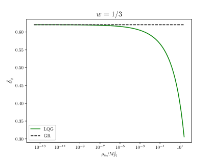
This reduction of should be related with a smaller cosmological/sound horizon in LQC compared to GR as it can be speculated from Eq. (3.14). To see this, let us find the necessary conditions to get a cosmological horizon in LQC smaller than that in GR. Doing so, one should require that
| (4.1) |
For and as given by Eq. (3.9) one can verify that the inequality 4.1 is identically satisfied. Thus, indeed the cosmological horizon in LQC is smaller than in GR leading to a reduction of compared to its GR value.
At this point, it is important to highlight that the PBH formation threshold depends as well, as already mentioned in the Introduction, on the shape of the of power spectrum of the cosmological perturbations which collapsed to form PBHs [27], which can either lower or raise . In particular, a very narrow-peaked power spectrum tends to raise the threshold and potentially can counterbalance the reduction of within LQC. This should be carefully investigated by extracting the effect of the shape of the power spectrum of cosmological perturbations on within LQC, something which has not yet been studied in the literature and goes beyond the scope of this work. However, in general one expects a reduction in within LQC compared to the case of GR, unless one works with a particularly narrow matter power spectrum.
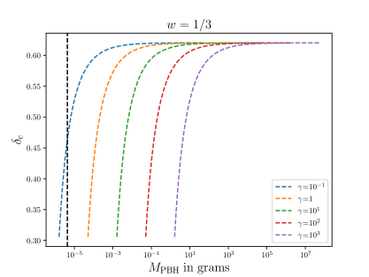
Then, we consider the Barbero-Immirzi parameter as a free parameter of the underlying quantum theory in the context of LQG. In particular, despite the fact that the Bekenstein-Hawking entropy has been standardly used as a way to fix the value of , the dependence of the entropy calculation on is controversial, and the value , calculated using thermodynamical arguments, is not broadly accepted [98, 99, 100]. In fact, the choice to vary this parameter is motivated by the fact that is actually a coupling constant with a topological term in the gravitational action, with no consequence at the level of the classical equations of motion [101, 102, 103, 104, 105, 106]. Thus, we vary the Barbero-Immirzi parameter within the range of accounting for observational constraints for the duration of inflation after a quantum bounce [107, 108]. At the end, we plot in the right panel of Fig. 1 the PBH formation threshold as a function of the PBH mass for different values of the parameter within the observationally allowed range . We set the lower bound on the PBH mass equal to the Planck mass as predicted within the quantum gravity approach [109] (See vertical black dashed line in the right panel of Fig. 1).
In order to get the PBH mass, we account for the fact that the PBH mass is of the order of the cosmological horizon mass at horizon crossing time. Solving at the end numerically Eq. (3.8) we found that . This corresponds to
| (4.2) |
passing from horizon crossing time up to the onset of the gravitational collapse process at , thus being in agreement with the results from PBH numerical simulations [110]. As expected, when we increase the value of the overall mass range moves to higher masses given the fact that higher values of are equivalent with lower values of , thus the quantum bounce happens at later times. Consequently, PBHs if formed will form at later times, thus will acquire larger masses.
Interestingly, independently on the value of the Barbero-Immirzi variable is reduced on the low mass region, which for corresponds to masses 555Recently, it was shown in [111, 112] that one-loop corrections to the renormalized primordial power spectrum rules out the possibility of having large mass PBHs within single-field inflationary models making the low-mass PBHs with very well motivated from the theoretical point of view. These very light PBHs can be naturally produced in LQG setups as discussed in [113].. In particular, this reduction in in this very small PBH mass range will be equivalent with an enhancement in their abundances, entailing in this way tremendous consequences on the phenomenology associated to ultra-light PBHs. Indicatively, we mention here that these ultra-light PBHs can trigger early PBH-matter dominated eras [114, 20, 21] before BBN and produce the DM relic abundance and the hot Standard Model (SM) plasma [115] reheating in this way the Universe through their evaporation [116]. Furthermore, they can account for the Hubble tension through the injection to the primordial plasma of light dark radiation degrees of freedom [117, 118] while at the same time they can produce naturally the baryon assymetry through CP violating out-of-equilibrium decays of their Hawking evaporation products [119, 120, 121]. Consequently, one can constrain the above mentioned observational/phenomenological signatures by studying PBH formation within the context of LQG while vice-versa given the above mentioned phenomenology one can constrain the Barbero-Immirzi parameter which is the fundamental parameter within LQG. In this way, PBHs are promoted as a novel probe to constrain the potential quantum nature of gravity.
5 Conclusions
PBHs firstly introduced in the ’70s are of great significance, since they can naturally account for a part or all of the dark matter sector, while at the same time they might seed the formation of large-scale structures through Poisson fluctuations. Moreover, they can also offer the seeds for the progenitors of the black-hole merging events recently detected by LIGO/VIRGO as well as for the supermassive black holes present in the galactic centers. Their formation was mainly studied within the context of general relativity using both analytic and numerical techniques.
In this work, we studied PBH formation within the context of LQC by investigating the impact of the potential quantum character of spacetime on the critical PBH formation threshold , whose value can crucially affect the abundance of PBHs, a quantity which is constrained by numerous observational probes. In particular, by comparing the gravitational force with the sound wave pressure force during the process of the gravitational collapse we obtained a reliable estimate on the value of .
Interestingly, we found that for low mass PBHs formed close to the quantum bounce, the value of is drastically reduced up to compared to the general relativistic regime with tremendous consequences for the observational/phenomenological footprints of such small PBH masses. In this way, we quantified for the first time to the best of our knowledge how quantum effects can influence PBH formation in the early Universe within a quantum gravity framework.
Finally, by treating the Barbero-Immirzi parameter as the free parameter of LQG we varied its value by studying its effect on the value of the PBH formation threshold. As expected, we found an overall shift of the PBH masses affected by the choice of . Very interestingly, we showed as well that using the observational and phenomenological signatures associated to ultra-light PBHs, namely the ones affected by LQG effects, one can constrain the quantum parameter . At this point, we should highlight the fact that our formalism can be applied to any quantum theory of gravity giving an explicit form for the equations of the background cosmic evolution establishing in this way the PBH portal as a novel probe to constrain the potential quantum nature of gravity.
Acknowledgments
The author acknowledges financial support from the Foundation for Education and European Culture in Greece as well the contribution of the COST Action CA18108 “Quantum Gravity Phenomenology in the multi-messenger approach”.
References
- [1] Y. B. Zel’dovich and I. D. Novikov, The Hypothesis of Cores Retarded during Expansion and the Hot Cosmological Model, Soviet Astronomy 10 (Feb., 1967) 602.
- [2] B. J. Carr and S. W. Hawking, Black holes in the early Universe, Mon. Not. Roy. Astron. Soc. 168 (1974) 399–415.
- [3] B. J. Carr, The primordial black hole mass spectrum., The Astrophysical Journal 201 (Oct., 1975) 1–19.
- [4] B. Carr and F. Kuhnel, Primordial Black Holes as Dark Matter: Recent Developments, 2006.02838.
- [5] A. M. Green and B. J. Kavanagh, Primordial Black Holes as a dark matter candidate, J. Phys. G 48 (2021) 043001, [2007.10722].
- [6] P. Meszaros, Primeval black holes and galaxy formation, Astron. Astrophys. 38 (1975) 5–13.
- [7] N. Afshordi, P. McDonald and D. Spergel, Primordial black holes as dark matter: The Power spectrum and evaporation of early structures, Astrophys. J. Lett. 594 (2003) L71–L74, [astro-ph/0302035].
- [8] B. J. Carr and M. J. Rees, How large were the first pregalactic objects?, Monthly Notices of the Royal Astronomical Society 206 (Jan., 1984) 315–325.
- [9] R. Bean and J. Magueijo, Could supermassive black holes be quintessential primordial black holes?, Phys. Rev. D 66 (2002) 063505, [astro-ph/0204486].
- [10] M. Safarzadeh, S. Naoz, A. Sadowski, L. Sironi and R. Narayan, Primordial black holes as seeds of magnetic fields in the universe, Mon. Not. Roy. Astron. Soc. 479 (2018) 315–318, [1701.03800].
- [11] T. Papanikolaou and K. N. Gourgouliatos, Primordial magnetic field generation via primordial black hole disks, 2301.10045.
- [12] T. Nakamura, M. Sasaki, T. Tanaka and K. S. Thorne, Gravitational waves from coalescing black hole MACHO binaries, Astrophys. J. 487 (1997) L139–L142, [astro-ph/9708060].
- [13] K. Ioka, T. Chiba, T. Tanaka and T. Nakamura, Black hole binary formation in the expanding universe: Three body problem approximation, Phys. Rev. D58 (1998) 063003, [astro-ph/9807018].
- [14] Y. N. Eroshenko, Gravitational waves from primordial black holes collisions in binary systems, J. Phys. Conf. Ser. 1051 (2018) 012010, [1604.04932].
- [15] J. L. Zagorac, R. Easther and N. Padmanabhan, GUT-Scale Primordial Black Holes: Mergers and Gravitational Waves, JCAP 1906 (2019) 052, [1903.05053].
- [16] M. Raidal, V. Vaskonen and H. Veermäe, Gravitational Waves from Primordial Black Hole Mergers, JCAP 1709 (2017) 037, [1707.01480].
- [17] E. Bugaev and P. Klimai, Induced gravitational wave background and primordial black holes, Phys. Rev. D 81 (2010) 023517, [0908.0664].
- [18] R. Saito and J. Yokoyama, Gravitational-wave background as a probe of the primordial black-hole abundance, Physical Review Letters 102 (Apr, 2009) .
- [19] T. Nakama and T. Suyama, Primordial black holes as a novel probe of primordial gravitational waves, Physical Review D 92 (Dec, 2015) .
- [20] T. Papanikolaou, V. Vennin and D. Langlois, Gravitational waves from a universe filled with primordial black holes, JCAP 03 (2021) 053, [2010.11573].
- [21] G. Domènech, C. Lin and M. Sasaki, Gravitational wave constraints on the primordial black hole dominated early universe, JCAP 04 (2021) 062, [2012.08151].
- [22] T. Papanikolaou, Gravitational waves induced from primordial black hole fluctuations: the effect of an extended mass function, JCAP 10 (2022) 089, [2207.11041].
- [23] G. Domènech, Scalar Induced Gravitational Waves Review, Universe 7 (2021) 398, [2109.01398].
- [24] T. Papanikolaou, C. Tzerefos, S. Basilakos and E. N. Saridakis, Scalar induced gravitational waves from primordial black hole Poisson fluctuations in f(R) gravity, JCAP 10 (2022) 013, [2112.15059].
- [25] T. Papanikolaou, C. Tzerefos, S. Basilakos and E. N. Saridakis, No constraints for f(T) gravity from gravitational waves induced from primordial black hole fluctuations, Eur. Phys. J. C 83 (2023) 31, [2205.06094].
- [26] S. Clesse and J. García-Bellido, Seven hints for primordial black hole dark matter, Physics of the Dark Universe 22 (Dec., 2018) 137–146, [1711.10458].
- [27] C. Germani and I. Musco, Abundance of Primordial Black Holes Depends on the Shape of the Inflationary Power Spectrum, Phys. Rev. Lett. 122 (2019) 141302, [1805.04087].
- [28] I. Musco, Threshold for primordial black holes: Dependence on the shape of the cosmological perturbations, Phys. Rev. D 100 (2019) 123524, [1809.02127].
- [29] A. Escrivà, C. Germani and R. K. Sheth, Universal threshold for primordial black hole formation, Phys. Rev. D 101 (2020) 044022, [1907.13311].
- [30] I. Musco, V. De Luca, G. Franciolini and A. Riotto, Threshold for primordial black holes. II. A simple analytic prescription, Phys. Rev. D 103 (2021) 063538, [2011.03014].
- [31] A. Escrivà, C. Germani and R. K. Sheth, Analytical thresholds for black hole formation in general cosmological backgrounds, JCAP 01 (2021) 030, [2007.05564].
- [32] B. J. Carr, The Primordial black hole mass spectrum, Astrophys. J. 201 (1975) 1–19.
- [33] T. Harada, C.-M. Yoo and K. Kohri, Threshold of primordial black hole formation, Phys. Rev. D88 (2013) 084051, [1309.4201].
- [34] T. Papanikolaou, Toward the primordial black hole formation threshold in a time-dependent equation-of-state background, Phys. Rev. D 105 (2022) 124055, [2205.07748].
- [35] B. Carr, K. Kohri, Y. Sendouda and J. Yokoyama, Constraints on primordial black holes, Rept. Prog. Phys. 84 (2021) 116902, [2002.12778].
- [36] B. J. Carr and S. W. Hawking, Black holes in the early Universe, Monthly Notices of Royal Astronomic Society 168 (Aug., 1974) 399–416.
- [37] D. K. Nadezhin, I. D. Novikov and A. G. Polnarev, The hydrodynamics of primordial black hole formation, Soviet Astronomy 22 (Apr., 1978) 129–138.
- [38] G. V. Bicknell and R. N. Henriksen, Formation of primordial black holes., Astrophysics Journal 232 (Sept., 1979) 670–682.
- [39] I. D. Novikov and A. G. Polnarev, The Hydrodynamics of Primordial Black Hole Formation - Dependence on the Equation of State, Soviet Astronomy 24 (Apr., 1980) 147–151.
- [40] J. C. Niemeyer and K. Jedamzik, Near-critical gravitational collapse and the initial mass function of primordial black holes, Phys. Rev. Lett. 80 (1998) 5481–5484, [astro-ph/9709072].
- [41] M. Shibata and M. Sasaki, Black hole formation in the friedmann universe: Formulation and computation in numerical relativity, Physical Review D 60 (Sep, 1999) .
- [42] M. Kawasaki and H. Nakatsuka, Effect of nonlinearity between density and curvature perturbations on the primordial black hole formation, Phys. Rev. D 99 (2019) 123501, [1903.02994].
- [43] S. Young, I. Musco and C. T. Byrnes, Primordial black hole formation and abundance: contribution from the non-linear relation between the density and curvature perturbation, JCAP 11 (2019) 012, [1904.00984].
- [44] V. De Luca, G. Franciolini, A. Kehagias, M. Peloso, A. Riotto and C. Ünal, The Ineludible non-Gaussianity of the Primordial Black Hole Abundance, JCAP 07 (2019) 048, [1904.00970].
- [45] C. Germani and R. K. Sheth, Nonlinear statistics of primordial black holes from Gaussian curvature perturbations, Phys. Rev. D 101 (2020) 063520, [1912.07072].
- [46] S. Young and M. Musso, Application of peaks theory to the abundance of primordial black holes, JCAP 11 (2020) 022, [2001.06469].
- [47] S. Young and C. T. Byrnes, Primordial black holes in non-Gaussian regimes, JCAP 1308 (2013) 052, [1307.4995].
- [48] S. Young, D. Regan and C. T. Byrnes, Influence of large local and non-local bispectra on primordial black hole abundance, JCAP 1602 (2016) 029, [1512.07224].
- [49] G. Franciolini, A. Kehagias, S. Matarrese and A. Riotto, Primordial Black Holes from Inflation and non-Gaussianity, JCAP 03 (2018) 016, [1801.09415].
- [50] C.-M. Yoo, J.-O. Gong and S. Yokoyama, Abundance of primordial black holes with local non-Gaussianity in peak theory, JCAP 09 (2019) 033, [1906.06790].
- [51] A. Kehagias, I. Musco and A. Riotto, Non-Gaussian Formation of Primordial Black Holes: Effects on the Threshold, JCAP 12 (2019) 029, [1906.07135].
- [52] F. Kühnel and M. Sandstad, Ellipsoidal collapse and primordial black hole formation, Phys. Rev. D 94 (2016) 063514, [1602.04815].
- [53] C.-M. Yoo, T. Harada and H. Okawa, Threshold of Primordial Black Hole Formation in Nonspherical Collapse, Phys. Rev. D 102 (2020) 043526, [2004.01042].
- [54] I. Musco and T. Papanikolaou, Primordial black hole formation for an anisotropic perfect fluid: Initial conditions and estimation of the threshold, Phys. Rev. D 106 (2022) 083017, [2110.05982].
- [55] T. Harada, K. Kohri, M. Sasaki, T. Terada and C.-M. Yoo, Threshold of Primordial Black Hole Formation against Velocity Dispersion in Matter-Dominated Era, 2211.13950.
- [56] C.-Y. Chen, Threshold of primordial black hole formation in Eddington-inspired-Born–Infeld gravity, Int. J. Mod. Phys. D 30 (2021) 02, [1912.10690].
- [57] C. Rovelli, Loop quantum gravity, Living Rev. Rel. 1 (1998) 1, [gr-qc/9710008].
- [58] A. Ashtekar, Introduction to loop quantum gravity and cosmology, Lect. Notes Phys. 863 (2013) 31–56, [1201.4598].
- [59] P. Singh, Are loop quantum cosmos never singular?, Class. Quant. Grav. 26 (2009) 125005, [0901.2750].
- [60] A. Ashtekar and D. Sloan, Loop quantum cosmology and slow roll inflation, Phys. Lett. B 694 (2011) 108–112, [0912.4093].
- [61] M. Bojowald, H. Hernandez, M. Kagan, P. Singh and A. Skirzewski, Formation and Evolution of Structure in Loop Cosmology, Phys. Rev. Lett. 98 (2007) 031301, [astro-ph/0611685].
- [62] P. Wu and S. N. Zhang, Cosmological evolution of interacting phantom (quintessence) model in Loop Quantum Gravity, JCAP 06 (2008) 007, [0805.2255].
- [63] S. Chen, B. Wang and J. Jing, Dynamics of interacting dark energy model in Einstein and Loop Quantum Cosmology, Phys. Rev. D 78 (2008) 123503, [0808.3482].
- [64] X. Fu, H. W. Yu and P. Wu, Dynamics of interacting phantom scalar field dark energy in Loop Quantum Cosmology, Phys. Rev. D 78 (2008) 063001, [0808.1382].
- [65] D. Dwivedee, B. Nayak, M. Jamil and L. P. Singh, Evolution of Primordial Black Holes in Loop Quantum Gravity, J. Astrophys. Astron. 35 (2014) 97–106, [1110.6350].
- [66] A. Ashtekar and J. Lewandowski, Background independent quantum gravity: A Status report, Class. Quant. Grav. 21 (2004) R53, [gr-qc/0404018].
- [67] T. Thiemann, Modern Canonical Quantum General Relativity. Cambridge Monographs on Mathematical Physics. Cambridge University Press, 2007, 10.1017/CBO9780511755682.
- [68] A. Ashtekar, M. Bojowald and J. Lewandowski, Mathematical structure of loop quantum cosmology, Adv. Theor. Math. Phys. 7 (2003) 233–268, [gr-qc/0304074].
- [69] M. Han, W. Huang and Y. Ma, Fundamental structure of loop quantum gravity, Int. J. Mod. Phys. D 16 (2007) 1397–1474, [gr-qc/0509064].
- [70] T. Thiemann, Quantum spin dynamics (QSD), Class. Quant. Grav. 15 (1998) 839–873, [gr-qc/9606089].
- [71] J. Yang and Y. Ma, New Hamiltonian constraint operator for loop quantum gravity, Phys. Lett. B 751 (2015) 343–347, [1507.00986].
- [72] A. Ashtekar and M. Campiglia, On the Uniqueness of Kinematics of Loop Quantum Cosmology, Class. Quant. Grav. 29 (2012) 242001, [1209.4374].
- [73] J. Engle, M. Hanusch and T. Thiemann, Uniqueness of the Representation in Homogeneous Isotropic LQC, Commun. Math. Phys. 354 (2017) 231–246, [1609.03548].
- [74] J. Lewandowski, A. Okolow, H. Sahlmann and T. Thiemann, Uniqueness of diffeomorphism invariant states on holonomy-flux algebras, Commun. Math. Phys. 267 (2006) 703–733, [gr-qc/0504147].
- [75] C. Fleischhack, Representations of the Weyl algebra in quantum geometry, Commun. Math. Phys. 285 (2009) 67–140, [math-ph/0407006].
- [76] A. Ashtekar, T. Pawlowski and P. Singh, Quantum Nature of the Big Bang: Improved dynamics, Phys. Rev. D 74 (2006) 084003, [gr-qc/0607039].
- [77] A. Ashtekar, Loop Quantum Cosmology: An Overview, Gen. Rel. Grav. 41 (2009) 707–741, [0812.0177].
- [78] A. Corichi and E. Montoya, Coherent semiclassical states for loop quantum cosmology, Phys. Rev. D 84 (2011) 044021, [1105.5081].
- [79] A. Corichi and E. Montoya, On the Semiclassical Limit of Loop Quantum Cosmology, Int. J. Mod. Phys. D 21 (2012) 1250076, [1105.2804].
- [80] G. J. Olmo and P. Singh, Effective Action for Loop Quantum Cosmology a la Palatini, JCAP 01 (2009) 030, [0806.2783].
- [81] G. Date and S. Sengupta, Effective Actions from Loop Quantum Cosmology: Correspondence with Higher Curvature Gravity, Class. Quant. Grav. 26 (2009) 105002, [0811.4023].
- [82] T. P. Sotiriou, Covariant Effective Action for Loop Quantum Cosmology from Order Reduction, Phys. Rev. D 79 (2009) 044035, [0811.1799].
- [83] A. Ashtekar and P. Singh, Loop Quantum Cosmology: A Status Report, Class. Quant. Grav. 28 (2011) 213001, [1108.0893].
- [84] A. Ashtekar, T. Pawlowski, P. Singh and K. Vandersloot, Loop quantum cosmology of k=1 FRW models, Phys. Rev. D 75 (2007) 024035, [gr-qc/0612104].
- [85] A. Corichi and A. Karami, Loop quantum cosmology of k=1 FRW: A tale of two bounces, Phys. Rev. D 84 (2011) 044003, [1105.3724].
- [86] M. Motaharfar and P. Singh, Role of dissipative effects in the quantum gravitational onset of warm Starobinsky inflation in a closed universe, Phys. Rev. D 104 (2021) 106006, [2102.09578].
- [87] V. Taveras, Corrections to the Friedmann Equations from LQG for a Universe with a Free Scalar Field, Phys. Rev. D 78 (2008) 064072, [0807.3325].
- [88] J. L. Willis, On the low-energy ramifications and a mathematical extension of loop quantum gravity, other thesis, 2004.
- [89] P. Singh, K. Vandersloot and G. V. Vereshchagin, Non-singular bouncing universes in loop quantum cosmology, Phys. Rev. D 74 (2006) 043510, [gr-qc/0606032].
- [90] G. Calcagni and G. M. Hossain, Loop quantum cosmology and tensor perturbations in the early universe, Adv. Sci. Lett. 2 (2009) 184, [0810.4330].
- [91] J. Mielczarek, Perturbations in loop quantum cosmology. PhD thesis, Jagiellonian U. (main), 2012.
- [92] K. A. Meissner, Black hole entropy in loop quantum gravity, Class. Quant. Grav. 21 (2004) 5245–5252, [gr-qc/0407052].
- [93] L. L. Graef, R. O. Ramos and G. S. Vicente, Gravitational particle production in loop quantum cosmology, Phys. Rev. D 102 (2020) 043518, [2007.02395].
- [94] G. S. Vicente, R. O. Ramos and L. L. Graef, Gravitational particle production and the validity of effective descriptions in loop quantum cosmology, Phys. Rev. D 106 (2022) 043518, [2207.00435].
- [95] A. Corichi and P. Singh, Quantum bounce and cosmic recall, Phys. Rev. Lett. 100 (2008) 161302, [0710.4543].
- [96] M. Bojowald, Quantum nature of cosmological bounces, Gen. Rel. Grav. 40 (2008) 2659–2683, [0801.4001].
- [97] J. Amorós, J. de Haro and S. D. Odintsov, Bouncing loop quantum cosmology from gravity, Phys. Rev. D 87 (2013) 104037, [1305.2344].
- [98] J. Engle, K. Noui, A. Perez and D. Pranzetti, Black hole entropy from an SU(2)-invariant formulation of Type I isolated horizons, Phys. Rev. D 82 (2010) 044050, [1006.0634].
- [99] E. Bianchi, Entropy of Non-Extremal Black Holes from Loop Gravity, 1204.5122.
- [100] P. J. Wong, Shape Dynamical Loop Gravity from a Conformal Immirzi Parameter, Int. J. Mod. Phys. D 26 (2017) 1750131, [1701.07420].
- [101] S. K. Asante, B. Dittrich and H. M. Haggard, Effective Spin Foam Models for Four-Dimensional Quantum Gravity, Phys. Rev. Lett. 125 (2020) 231301, [2004.07013].
- [102] L. Perlov, Barbero–Immirzi value from experiment, Mod. Phys. Lett. A 36 (2021) 2150192, [2005.14141].
- [103] B. Broda and M. Szanecki, A relation between the Barbero-Immirzi parameter and the standard model, Phys. Lett. B 690 (2010) 87–89, [1002.3041].
- [104] S. Mercuri and V. Taveras, Interaction of the Barbero-Immirzi Field with Matter and Pseudo-Scalar Perturbations, Phys. Rev. D 80 (2009) 104007, [0903.4407].
- [105] C. Pigozzo, F. S. Bacelar and S. Carneiro, On the value of the Immirzi parameter and the horizon entropy, Class. Quant. Grav. 38 (2021) 045001, [2001.03440].
- [106] S. Carneiro and C. Pigozzo, Quasinormal modes and horizon area quantisation in Loop Quantum Gravity, Gen. Rel. Grav. 54 (2022) 20, [2012.00227].
- [107] M. Benetti, L. Graef and R. O. Ramos, Observational Constraints on Warm Inflation in Loop Quantum Cosmology, JCAP 10 (2019) 066, [1907.03633].
- [108] L. N. Barboza, G. L. L. W. Levy, L. L. Graef and R. O. Ramos, Constraining the Barbero-Immirzi parameter from the duration of inflation in loop quantum cosmology, Phys. Rev. D 106 (2022) 103535, [2206.14881].
- [109] S. R. Coleman, J. Preskill and F. Wilczek, Quantum hair on black holes, Nucl. Phys. B378 (1992) 175–246, [hep-th/9201059].
- [110] I. Musco, J. C. Miller and L. Rezzolla, Computations of primordial black hole formation, Class. Quant. Grav. 22 (2005) 1405–1424, [gr-qc/0412063].
- [111] S. Choudhury, M. R. Gangopadhyay and M. Sami, No-go for the formation of heavy mass Primordial Black Holes in Single Field Inflation, 2301.10000.
- [112] S. Choudhury, S. Panda and M. Sami, No-go for PBH formation in EFT of single field inflation, 2302.05655.
- [113] L. Modesto and I. Premont-Schwarz, Self-dual Black Holes in LQG: Theory and Phenomenology, Phys. Rev. D 80 (2009) 064041, [0905.3170].
- [114] K. Inomata, K. Kohri, T. Nakama and T. Terada, Gravitational Waves Induced by Scalar Perturbations during a Gradual Transition from an Early Matter Era to the Radiation Era, JCAP 10 (2019) 071, [1904.12878].
- [115] O. Lennon, J. March-Russell, R. Petrossian-Byrne and H. Tillim, Black Hole Genesis of Dark Matter, JCAP 04 (2018) 009, [1712.07664].
- [116] J. Martin, T. Papanikolaou and V. Vennin, Primordial black holes from the preheating instability in single-field inflation, JCAP 01 (2020) 024, [1907.04236].
- [117] D. Hooper, G. Krnjaic and S. D. McDermott, Dark Radiation and Superheavy Dark Matter from Black Hole Domination, JHEP 08 (2019) 001, [1905.01301].
- [118] S. Nesseris, D. Sapone and S. Sypsas, Evaporating primordial black holes as varying dark energy, Phys. Dark Univ. 27 (2020) 100413, [1907.05608].
- [119] J. D. Barrow, E. J. Copeland, E. W. Kolb and A. R. Liddle, Baryogenesis in extended inflation. 2. Baryogenesis via primordial black holes, Phys. Rev. D 43 (1991) 984–994.
- [120] N. Bhaumik, A. Ghoshal and M. Lewicki, Doubly peaked induced stochastic gravitational wave background: testing baryogenesis from primordial black holes, JHEP 07 (2022) 130, [2205.06260].
- [121] T. C. Gehrman, B. Shams Es Haghi, K. Sinha and T. Xu, Baryogenesis, Primordial Black Holes and MHz-GHz Gravitational Waves, 2211.08431.