Efficiently predicting high resolution mass spectra
with graph neural networks

Abstract

Identifying a small molecule from its mass spectrum is the primary open problem in computational metabolomics. This is typically cast as information retrieval: an unknown spectrum is matched against spectra predicted computationally from a large database of chemical structures. However, current approaches to spectrum prediction model the output space in ways that force a tradeoff between capturing high resolution mass information and tractable learning. We resolve this tradeoff by casting spectrum prediction as a mapping from an input molecular graph to a probability distribution over molecular formulas. We discover that a large corpus of mass spectra can be closely approximated using a fixed vocabulary constituting only $2\%$ of all observed formulas. This enables efficient spectrum prediction using an architecture similar to graph classification – GrAFF-MS – achieving significantly lower prediction error and orders-of-magnitude faster runtime than state-of-the-art methods.

1 Introduction

The identification of unknown small molecules in complex chemical mixtures is a primary challenge in many areas of chemical and biological science. The standard high-throughput approach to small molecule identification is tandem mass spectrometry (MS/MS), with diverse applications including metabolomics [1], drug discovery [2], clinical diagnostics [3], forensics [4], and environmental monitoring [5].

The key bottleneck in MS/MS is structural elucidation: given a mass spectrum, we must determine the 2D structure of the molecule it represents. This problem is far from solved, and adversely impacts all areas of science that use MS/MS. Typically only $2{-}4\%$ of spectra are identified in untargeted metabolomics experiments [6], and a recent competition saw no more than 30% accuracy [7].

Because MS/MS is a lossy measurement, and existing training sets are small, direct prediction of structures from spectra is particularly challenging. Therefore the most common approach is spectral library search, which casts the problem as information retrieval [8]: an observed spectrum is queried against a library of spectra with known structures. This provides an informative prior, and has the advantage of easy interpretability as the entire space of solutions is known. As there are relatively few $(10^{4})$ small molecules with known experimental mass spectra, in spectral library search it is necessary to augment libraries with spectra predicted from large databases $(10^{6}-10^{9})$ of molecular graphs. This motivates the problem of spectrum prediction.

Spectrum prediction is actively studied in metabolomics and quantum chemistry [9], yet has received little attention from the machine learning community. A major challenge in spectrum prediction is modelling of the output space: a mass spectrum is a variable-length set of real-valued ($m/z$, height) tuples, which is not straightforward to represent as an output of a deep learning model. The $m/z$ coordinate (mass-to-charge ratio) poses particular difficulty: it must be predicted with high precision, as a key strength of MS/MS is the ability to distinguish fractional $m/z$ differences on the order of $10^{-6}$ representative of different elemental composition.

Existing approaches to spectrum prediction force a tradeoff between capturing high-resolution $m/z$ information and tractability of the learning problem. Mass-binning methods [10, 11, 12] represent a spectrum as a fixed-length vector by discretizing the $m/z$ axis at regular intervals, discarding valuable information in favor of tractable learning. Bond-breaking methods [13, 14] achieve perfect $m/z$ resolution, but do so through expensive combinatorial enumeration of substructures.

This work makes the following contributions:

• We formulate spectrum prediction as a mapping from a molecular graph to a probability distribution over molecular formulas, allowing full resolution predictions without enumerating substructures;

• We discover most mass spectra can be effectively approximated with a small fixed vocabulary of molecular formulas, bypassing the tradeoff between $m/z$ resolution and tractable learning; and

• We implement an efficient graph neural network architecture, GrAFF-MS, that substantially outperforms state-of-the-art in both prediction error and runtime on two canonical mass spectrometry datasets.

2 Background

2.1 Definitions

We denote vectors $\bm{x}$ in bold lowercase and matrices $\bm{X}$ in bold uppercase.

A molecular graph $G=(V,E,\bm{a},\bm{b})$ is a minimal description of the structure of a molecule: comprising an undirected graph with node set $V$, edge set $E\subset V\times V$, node labels $\bm{a}\in[118]^{V}$ indicating atom number, and edge labels $\bm{b}\in(\{1,1.5,2,3\}\times\{-1,0,1\})^{E}$ indicating bond order and chirality.

A molecular formula $f$ (e.g. C₈H${}_{10}N_{4}O_{2}$) describes a multiset of atoms, which we encode as a nonnegative integer vector of atom counts in $\mathcal{F}^{*}\doteq\mathbb{Z}_{+}^{118}$. Formulas may be added and subtracted from one another, and inequalities between formulas are taken to hold elementwise. We reserve the symbol $P$ to indicate a formula of a precursor ion. The subformulas of $P$ are the set $\mathcal{F}(P)\doteq\{f\in\mathcal{F}^{*}:f\leq P\}$.

$\langle\mu,f\rangle\in\mathbb{R}_{+}$ is the theoretical mass of a molecule with formula $f$, with units of daltons (Da): this is a linear combination of the monoisotopic masses of the elements of the periodic table, $\mu\in\mathbb{R}_{+}^{118}$, with multiplicities given by $f$.

A mass spectrum $S$ is a variable-length set of peaks, each of which is a ($m/z$, height) tuple $(m_{i},y_{i})\in\mathbb{R}_{+}^{2}$. We use the notation $i\in S$ to index peaks in a spectrum. We assume spectra are normalized, permitting us to treat them as probability distributions: $\sum_{i\in S}{y_{i}}=1$. A mass spectrum is implicitly always accompanied by a precursor formula $P$.

We always assume charge $z\doteq 1$, as it is rare for small molecules to acquire more than a single charge.

2.2 Tandem mass spectrometry

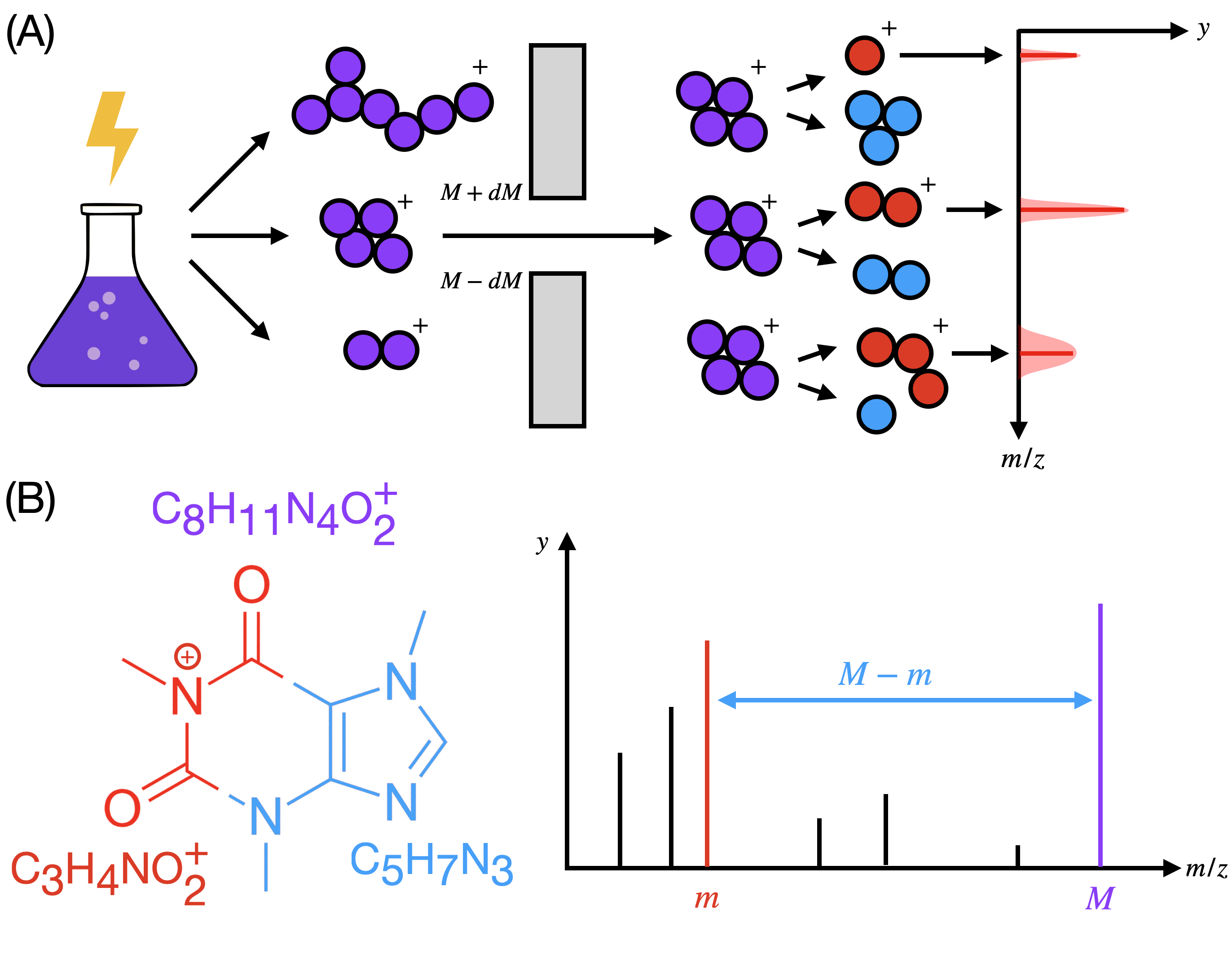
A tandem mass spectrometer is a scientific instrument that generates high-throughput experimental signatures of the molecules present in a complex mixture. It works by ionizing a chemical sample into a jet of electrically-charged gas. This gas is electromagnetically filtered to select a population of precursor ions of a specific mass-to-charge ratio ($m/z$) representing a unique molecular structure. Each precursor ion is fragmented by collision with molecules of an inert gas. If a collision occurs with sufficient energy, one or more bonds in the precursor will break, yielding a charged product ion and one or more uncharged neutral loss molecules. The product ion is measured by a detector, which records its $m/z$ up to a small measurement error proportional to the $m/z$ times the instrument resolution $\epsilon$. This process is repeated for large numbers of identical precursor ions, building up a histogram indexed by $m/z$. Local maxima in this histogram are termed peaks: ideally, each peak represents a unique product ion, with height reflecting its probability of formation. This set of peaks constitutes the mass spectrum. A typical mass spectrometry experiment acquires mass spectra for tens of thousands of distinct precursors in this manner, with $m/z$s measured at resolution on the order of $10^{-6}$. This process is depicted in Figure 1A; we illustrate the relationship between precursor ion, product ion, and neutral loss in Figure 1B.

Figure 1: (A) The workflow of tandem mass spectrometry. A chemical mixture is ionized and filtered to isolate precursor ions of $m/z=M$; these are fragmented into product ions (red) and neutral losses (blue), and a detector yields a histogram of product ions indexed by $m/z$, with measurement error proportional to $m/z$. (B) An example fragmentation of a precursor ion with formula C₈H₁₁N₄O₂. Fragmentation breaks bonds, cutting the molecular graph into connected components. The component retaining the charge is the product ion; its complement is the neutral loss. The peak at $m/z=m$ represents the product ion; given the precursor formula, we can equally specify this peak by its formula C₃H₄NO₂, or the formula of its neutral loss C₅H₇N₃.

2.3 Structural elucidation

A tandem mass spectrum of a molecule contains substantial information about its 2D structure. Peak heights reflect the propensity of different bonds to break: this can reveal structural differences in compounds, even if they have the same molecular formula. Furthermore, the $O(10^{-6})$ resolution of modern MS/MS can detect small characteristic deviations from integrality in the masses of individual chemical elements that arise from nuclear physics, allowing detailed information about the molecular formula to be inferred from the spectrum with high accuracy (Sec 2.4).

The task of inferring a 2D structure from a mass spectrum, structural elucidation, is the major open problem in computational metabolomics, dating back to the 1960s in one of the earliest examples of an expert system [15]. Yet structural elucidation remains far from solved: despite half a century of research, algorithmic approaches perform only marginally better than manual annotations by expert chemists, with no method submitted to the 2022 Critical Analysis of Small Molecule Identification (CASMI) challenge exceeding $30\%$ accuracy [7].

The difficulty of structural elucidation has broad scientific implications: while a modern metabolomics experiment routinely detects tens of thousands of spectra, usually only a few percent of these are confidently annotated with a structure [6]. Spectral library search, described in the introduction, is the approach to structural elucidation preferred in practice by most biologists and chemists [8], and is a standard component of existing metabolomics workflows. The availability of high-quality predicted spectra across large chemical structure databases would therefore greatly increase compound identification rates in real experimental settings.

2.4 Mass decomposition

Modern mass spectrometry achieves sufficiently high resolution to detect small deviations in $m/z$ from integrality that are characteristic of different chemical elements. This property is a key strength of the technology, because it permits annotating peaks with formulas through mass decomposition [16]. Given a product ion of $m/z=m$, a precursor formula $P$, and an instrument resolution $\epsilon$, product mass decomposition yields a set $\mathcal{F}(P,m,\epsilon)$ of chemically plausible subformulas of $P$ whose theoretical masses lie within measurement error $\epsilon m$ of $m$. This can be cast as an integer program, in which all solutions of the following minimization with cost $\leq\epsilon m$ are enumerated:

$$\min_{f\in\mathcal{F}^{*}} \ |\langle\mu,f\rangle-m|$$ (1)

s.t. $$\ f\leq P,f\in\Omega$$ (2)

where $\Omega$ describes a general set of constraints that exclude unrealistic molecular formulas [17]. In practice, with modern instruments $\epsilon$ is sufficiently small for there to typically be only one or a few solutions to this optimization. This allows us to later rely on product mass decomposition as a black-box to generate useful formula annotations at training time.

3 Related work

Bond-breaking, used in [13, 14, 18], solves the problem of representing the output space by enumerating the 2D structures of all probable product ions. These are taken to be connected subgraphs of the precursor, generated by sequences of edge removals. Each product ion structure is scored for its probability of formation, and a spectrum is generated by associating this probability with each structure’s theoretical $m/z$. Bond-breaking therefore achieves perfect $m/z$ resolution, but suffers from two major weaknesses: first, enumerating substructures scales poorly with molecule size, and is not conducive to massively-parallel implementation on a GPU. We found a state-of-the-art method [13] takes ${\sim}5$s on average to predict a single mass spectrum, which precludes training on the largest available datasets: using the same settings as its authors, training [13] on $\sim$300k spectra in NIST-20 would take an estimated three months on a 64-core machine. It also poses serious limitations at test time, as inference with a large-scale structure database like ChEMBL [19] requires predicting millions of spectra. The other weakness of bond-breaking arises from a restrictive modelling assumption: rearrangement reactions [20] frequently yield product ions that are not reachable from the precursor by sequences of edge removals.

Mass-binning is used for spectrum prediction by [10], and subsequently employed in recent preprints [11, 12]. This approach represents a mass spectrum as a fixed-length vector via discretization: the m/z axis is partitioned into narrow regularly-spaced bins, and each bin is assigned the sum of the intensities of all peaks falling within its endpoints. Spectrum prediction then becomes a vector-valued regression problem. Mass-binning is conducive to GPU implementation and scales better than bond-breaking, but because a target space with millions of mass bins is too large, realistic bin counts lose essential high resolution information about the molecular formulas of the peaks: discarding a key strength of MS/MS analysis in favor of a tractable learning problem. Such models are also susceptible to edge effects, where $m/z$ measurement error of the instrument can cause peaks of the same product ion to cross bin boundaries from spectrum to spectrum.

Other approaches include molecular dynamics simulation [21], which has extremely high computational costs; and NLP-inspired models for peptides [22, 23], which are effective but inapplicable to other types of molecules.

4 GrAFF-MS

Our approach constitutes three major components: first, we represent the output space of spectrum prediction as a space of probability distributions over molecular formulas. We then introduce a constant-sized approximation of this output space using a fixed vocabulary of formulas, which we can generate from our training data; we later show this introduces only minor approximation cost, as most formulas occur with low probability. Finally, we derive a loss function that takes into account data-specific ambiguities introduced by our model of the output space. These components together allow us to efficiently predict spectra using a standard graph neural network architecture. We call our approach GrAFF-MS: (Gr)aph neural network for (A)pproximation via (F)ixed (F)ormulas of (M)ass (S)pectra.

4.1 Modelling spectra as probability distributions over molecular subformulas of the precursor

Our aim is to predict a mass spectrum from a molecular graph. To do so, we must determine how to best represent the output space: a spectrum comprises a variable-length set of peaks located at continuous $m/z$ positions, whose heights sum to one. We notice that peaks are not located arbitrarily: the set of $m/z$s is structured, as the $m/z$ of a peak is determined (up to measurement error) by the molecular formula of its corresponding product ion. This formula is sufficient to determine the $m/z$; in particular, we do not need to know the product ion’s full 2D structure. We therefore model a mass spectrum as a probability distribution over molecular subformulas $\mathcal{F}(P)$ of the precursor $P$:

$$S =\{(m_{f},y_{f}):f\in\mathcal{F}(P)\}$$ (3)

where $m_{f}\doteq\langle\mu,f\rangle$ is the theoretical mass of formula $f$.

This is more efficient in principle than bond-breaking, which models a spectrum as a distribution over at worst exponentially many substructures of the precursor. But the number of subformulas is only polynomial in the coefficients of the precursor formula – and the majority of subformulas can be ruled out a priori as chemically infeasible [17]. It is also less restrictive than bond-breaking, which relies on hand-engineered rules to capture rearrangement reactions: enumerating subformulas is guaranteed to generate all possible peaks, irrespective of whether the structure of their product ion is reachable by edge removals or not. Yet our approach preserves the core advantage of bond-breaking over mass-binning: predicting a height for each subformula yields spectra with perfect $m/z$ resolution.

4.2 Fixed-vocabulary approximation of formula space

In practice, enumeration of subformulas is still a costly operation for larger molecules. One way to avoid this would be to sequentially decode formulas of nonzero probability one at a time: we opt not to do so, as this requires a more complex, data-hungrier model, and necessitates a linear ordering of formulas, for which there is not an obvious correct choice. Instead, we exploit a property of small molecule mass spectra that we discovered in this work, and illustrate in Figure 2 of the results: almost all of the signal in small molecule mass spectra lies in peaks that can be explained by a relatively small number $({\sim}2\%)$ of product ion and neutral loss formulas that frequently recur across spectra.

Inspired by this finding, we approximate $\mathcal{F}(P)$ via the union $\hat{\mathcal{F}}(P)=\hat{\mathcal{P}}\cup(P-\hat{\mathcal{L}})$ of a fixed set of frequent product ion formulas $\hat{\mathcal{P}}$, and a variable set of ‘precursor-specific’ formulas $P-\hat{\mathcal{L}}$ obtained by subtracting a fixed set of frequent neutral loss formulas $\hat{\mathcal{L}}$ from the precursor $P$. This greatly simplifies the spectrum prediction problem: we now only need to predict a probability for each of the formulas in $\hat{\mathcal{P}}$ and $\hat{\mathcal{L}}$, which we can accomplish with time constant in the size of the precursor.

Stated explicitly, we approximate the spectrum as:

$$S\approx\{(m_{f},y_{f}):f\in\hat{\mathcal{F}}(P)\}$$ (4)

where a height of zero is implicitly assigned to any formula not in $\hat{\mathcal{F}}(P)$.

The fact that we can equally represent a product ion by either its own formula or a neutral loss formula relative to its precursor ion is crucial to generalization. If we only included frequent product ion formulas, we would explain peaks of low mass well, which typically correspond to small charged functional groups. But as formula space becomes larger with increasing mass, it becomes increasingly unlikely that every significant peak of higher mass in an unseen compound will be explained. However such peaks do not represent arbitrary subformulas of the precursor: they tend to arise from losses of small uncharged functional groups and combinations thereof, which we capture by including frequent neutral losses.

Our algorithm to generate $\hat{\mathcal{P}}$ and $\hat{\mathcal{L}}$ involves listing all product ion and neutral loss formulas yielded by mass decomposition of the training set, and ranking them by the sum of the heights of all peaks to which each formula is assigned; we select the top $K$ highest ranked among either type. Pseudocode is provided in appendix A.

4.3 Peak-marginal cross entropy

To train our approach, we must rely on formula annotations generated by mass decomposition. Because mass spectrometers have limited resolution, it is often the case that more than one valid subformula has a mass within measurement error of a peak. These are considered equiprobable a priori, and need not be mutually exclusive: it is possible for a compound to contain two distinct substructures with $m/z$ difference smaller than the measurement error. As we cannot pick a single formula in such cases, we approximate the full cross entropy by marginalizing over compatible formulas: this yields the peak-marginal cross entropy, which we minimize w.r.t. the parameters of a neural network $\hat{\bm{y}}(\cdot;\theta)$:

$$\min_{\theta}\ -\sum_{n=1}^{N}\sum_{i\in S_{n}}y_{i}^{n}\log\sum_{f\in\hat{\mathcal{F}}^{n}_{i}}\hat{y}_{f}(G_{n};\theta)$$ (5)

using the shorthand $\hat{\mathcal{F}}^{n}_{i}\doteq\hat{\mathcal{F}}(P_{n})\cap\mathcal{F}(P_{n},m^{n}_{i},\epsilon)$ to indicate the intersection of our approximated vocabulary with the formula annotations generated by mass decomposition. We provide a derivation from first principles in appendix B.

In this formulation, given a molecular graph $G$ of a precursor with formula $P$, our model predicts a probability $\hat{y}_{f}$ for every formula $f$ in the fixed vocabulary. This produces a spectrum $\hat{S}=\{(m_{f},\hat{y}_{f}):f\in\hat{\mathcal{F}}(P)\}$. These per-formula probabilities are summed within each observed peak across its compatible formulas to yield a predicted peak height, and the cross-entropy between the observed and predicted peak heights across the entire spectrum is minimized.

4.4 Model architecture

Formulating spectrum prediction as graph classification permits a fairly typical GNN architecture. GrAFF-MS uses a graph isomorphism network with edge and graph Laplacian features [24, 25, 26]: this encodes the molecular graph into a dense vector representation, which is then conditioned on mass-spectral covariates and passed through a feed-forward network that decodes a logit for each formula in the vocabulary.

We start with the graph of the 2D structure $G=(V,E)$, to which we add a virtual node [27] and four classes of features: node features $\bm{a}_{i}\in\mathbb{R}^{d_{atom}}$, edge features $\bm{b}_{ij}\in\mathbb{R}^{d_{bond}}$, covariate features $\bm{c}\in\mathbb{R}^{d_{cov}}$, and the top eigenvectors and eigenvalues of the graph Laplacian $\bm{v}_{i}\in\mathbb{R}^{d_{eig}},\bm{\lambda}\in\mathbb{R}^{d_{eig}}$. We use the canonical atom and bond featurizers from DGL-LifeSci [28] to generate $\bm{a}$ and $\bm{b}$. Since a mass spectrum is not fully determined by the molecular graph, $\bm{c}$ includes a number of necessary experimental parameters: normalized collision energy, precursor ion type, instrument model, and presence of isotopic peaks. Further details are provided in Table 2 of the appendix; there we also provide hyperparameter settings.

We first embed the node, edge, and covariate features into $\mathbb{R}^{d_{enc}}$, reusing the following MLP block:

$$\texttt{MLP}(\cdot)=\texttt{LayerNorm}(\texttt{Dropout}(\texttt{SiLU}(\texttt{Linear}(\cdot))))$$

and transform the Laplacian features into node positional encodings in $\mathbb{R}^{d_{enc}}$ using a SignNet [26] with $\phi$ and $\rho$ both implemented as 2-layer stacked MLP blocks:

$$\bm{x}_{i}^{atom} =\texttt{MLP}_{atom}(\bm{a}_{i})$$ (6)

$$\bm{x}_{i}^{eig} =\texttt{SignNet}(\bm{v}_{i},\bm{\lambda})$$ (7)

$$\bm{x}_{ij}^{bond} =\texttt{MLP}_{bond}(\bm{b}_{ij})$$ (8)

$$\bm{x}^{cov} =\texttt{MLP}_{cov}(\bm{c})$$ (9)

taking $i\in V$ and $(i,j)\in E$. We sum the embedded atom features and node positional encodings, and pass these along with embedded bond features into a stack of alternating $L$ message-passing layers to update the node representations, and $L$ MLP layers to update the edge representations.

$$\bm{x}_{i}^{(0)} =\bm{x}_{i}^{atom}+\bm{x}_{i}^{eig}$$ (10)

$$\bm{e}_{ij}^{(0)} =\bm{x}_{ij}^{bond}$$ (11)

$$\bm{X}^{(l+1)} =\bm{X}^{(l)}+\texttt{GINEConv}^{(l)}(G,\bm{X}^{(l)},\bm{E}^{(l)})$$ (12)

$$\bm{e}_{ij}^{(l+1)} =\bm{e}_{ij}^{(l)}+\texttt{MLP}^{(l)}_{edge}(\bm{e}^{(l)}_{ij}\|\bm{x}^{(l+1)}_{i}\|\bm{x}^{(l+1)}_{j})$$ (13)

where $\|$ denotes concatenation. The message-passing layer uses the GINEConv operation implemented in [29]: for its internal feed-forward network, we use two stacked MLP blocks with GraphNorm [30] in place of layer normalization. We similarly replace layer normalization with GraphNorm in the $\texttt{MLP}_{edge}$ blocks. Both node and edge updates use residual connections, which we found greatly accelerate training.

We generate a dense representation of the molecule by attention pooling over nodes [31], to which we add the embedded covariate features. This is decoded by a feed-forward network into a spectrum representation $\bm{x}^{spec}\in\mathbb{R}^{d_{dec}}$.

$$a_{i} =\texttt{Softmax}_{i\in V}(\texttt{Linear}(\bm{x}_{i}))$$ (14)

$$\bm{x}^{mol} =\sum_{i\in V}a_{i}\bm{x}^{(L)}_{i}$$ (15)

$$\bm{x}^{spec} =\texttt{MLP}_{spec}(\bm{x}^{mol}+\bm{x}^{cov})$$ (16)

where $\texttt{MLP}_{spec}$ is a stack of $L^{\prime}$ MLP blocks with residual connections. In principle we may now project this representation via a linear layer $(\bm{w}_{k},b_{k})$ into a logit $z_{k}$ for each of the $K$ product ion or neutral loss formulas in the vocabulary.

4.5 Domain-specific modifications

We must now introduce a number of corrections motivated by domain knowledge to produce realistic mass spectra.

Following fragmentation, certain product ions can bind ambient water or nitrogen molecules as adducts, shifting the mass of the fragment. This occurrence is annotated in our training set. For each formula in our vocabulary, we therefore predict a logit for three different adduct states of the fragment, indexed by $\alpha$: the original product ion $f$, $f$ $+$ H₂O, and $f$ $+$ N₂. In effect this triples our vocabulary size.

Depending upon instrument parameters, tandem mass spectra can display small peaks arising from higher isotopic states of the precursor ion, at integral $m/z$ shifts relative to the monoisotopic peak. Isotopic state is independent of fragmentation: so rather than expanding our vocabulary again, we apply to all predictions a shared offset for each isotopic state $\beta\in\{0,1,2\}$, which we parameterize on $\bm{x}^{spec}$.

As our vocabulary includes both product ions and neutral losses, we must deal with occasional double-counting: depending on the precursor $P$, there are cases where the same subformula $f$ will be predicted both as a product ion ($f\in\hat{\mathcal{P}}$) and a neutral loss ($P-f\in\hat{\mathcal{L}}$). In such cases – denoted by the set $\hat{\mathcal{D}}(P)$ – we subtract a $\log 2$ correction factor from both logits: this way the innermost summation in Equation 5 takes the mean of their contributions instead of their sum.

Applying these corrections and softmaxing yields the final heights of the predicted mass spectrum $\hat{\bm{y}}$:

$$z_{k}^{\alpha\beta} =\bm{w}_{k}^{\alpha}\bm{x}^{spec}+\bm{w}^{\beta}\bm{x}^{spec}+b_{k}^{\alpha}$$ (17)

$$-\mathbb{I}[k\in\hat{\mathcal{D}}(P)]\log 2$$ (18)

$$\hat{y}_{k}^{\alpha\beta} =\texttt{Softmax}_{k,\alpha,\beta}(z_{k}^{\alpha\beta})$$ (19)

5 Experiments

5.1 Datasets

5.1.1 NIST-20

We train our model on the NIST-20 tandem MS spectral library [32]. This is the largest dataset of high resolution mass spectra of small molecules, curated by expert chemists, and is commercially available for a modest fee. For each measured compound, NIST-20 provides typically several spectra acquired across a range of collision energies. Each spectrum is represented as a list of ($m/z$, intensity, annotation) peak tuples, in addition to metadata describing instrumental parameters and compound identity. The annotation field includes a list of formula hypotheses per peak that were computed via mass decomposition.

We restrict NIST-20 to HCD spectra with $[M+H]^{+}$ or $[M-H]^{-}$ precursor ions. We exclude structures that are annotated as glycans or peptides or exceed 1000Da in mass (as these are not typically considered small molecules), or have atoms other than {C, H, N, O, P, S, F, Cl, Br, I}.

We use an $85/5/10$ structure-disjoint train/validation/test split, which we generate by grouping spectra according to the connectivity substring of their InChiKey [34] and assigning spectra to splits an entire group at a time. As CFM-ID only predicts monoisotopic spectra at qualitative energy levels {low, medium, high}, we restrict the test set to spectra with corresponding energies $\{20,35,50\}$ in which no peaks were annotated as higher isotopes. This yields 306,135 (19,871) training, 17,987 (1,167) validation, and 4,548 (1,637) test spectra (structures).

5.1.2 CASMI-16

It is well known that uniform train-test splitting can overestimate generalization in molecular machine learning [35]. To address this issue, we employ an independent test set: the spectra of the 2016 CASMI challenge [36]. This is a small public-domain mass spectrometry dataset, constructed by domain experts specifically for testing algorithms, and comprises structures selected as representative of those encountered ‘in the wild’ when performing mass spectrometry of small molecules.

We use $[M+H]^{+}$ and $[M-H]^{-}$ spectra from the combined ‘Training’ and ‘Challenge’ splits from Categories 2 and 3 of the challenge. We exclude any structures from CASMI-16 with an InChiKey connectivity match to any in NIST-20, yielding $156$ spectra of $141$ structures. The collision energy stepping protocol used in CASMI-16 is simulated by predicting a spectrum at each of $\{20,35,50\}$ normalized collision energy and returning their mean.

5.2 Baselines

5.2.1 CFM-ID

CFM-ID [13] is a bond-breaking method, viewed by the mass spectrometry community as the state-of-the-art in spectrum prediction [9]. We found CFM-ID prohibitively expensive to train on NIST-20 (one parallelized EM iterate on a subset of $\sim$60k spectra took 10 hours on a 64-core machine) so we use trained weights provided by its authors, learned from 18,282 spectra in the commercial METLIN dataset [37]. Domain experts consider spectra acquired under METLIN’s conditions interchangeable with those of NIST-20 [38] so it is reasonable to evaluate their model on our data.

5.2.2 NEIMS

NEIMS [10] is a feed-forward network that inputs a precomputed molecular fingerprint and outputs a mass-binned spectrum, which is postprocessed using a domain-specific gating operation. We retrained NEIMS on NIST-20, which necessitated two modifications: (1) we concatenate a vector of covariates to the fingerprint vector, without which NIST-20 spectra are not fully determined; and (2) we bin at 0.1Da intervals instead of 1Da intervals, to account for finer instrument resolution in NIST-20. We otherwise use the same hyperparameter settings as the original paper, and early-stop on validation loss.

5.3 Evaluation metrics

We quantify predictive performance using mass-spectral cosine similarity, which compares spectra subject to $m/z$ measurement error [39] by matching pairs of peaks. For two spectra $S$ and $\hat{S}$, mass-spectral cosine similarity $C_{S,\hat{S}}$ is the value of the following linear sum assignment problem:

$$C_{S,\hat{S}}\doteq\max_{x_{ij}\in\{0,1\}} \sum_{\begin{subarray}{c}i\in S,\ j\in\hat{S}:\\ |m_{i}-\hat{m}_{j}|\leq\tau\end{subarray}}x_{ij}\frac{y_{i}}{\|y\|_{2}}\frac{\hat{y}_{j}}{\|\hat{y}\|_{2}}$$ (20)

s.t. $$\textstyle\sum_{i\in S}x_{ij}\leq 1$$ (21)

$$\textstyle\sum_{j\in\hat{S}}x_{ij}\leq 1$$ (22)

We use the CosineHungarian implementation in the matchms Python package, with tolerance $\tau=0.05$. We report mean cosine similarity across spectra, as well as the fraction of spectra scoring $>0.7$, which is commonly employed in spectral library search as a heuristic cutoff for a positive match [40].

We also compare runtime of GrAFF-MS against the bond-breaking method CFM-ID. For fair comparison, we time a forward pass for each structure in the NIST-20 test split using only the CPU, without any batching. We include time spent in preprocessing: our input is a SMILES string and experimental covariates, and our output is a spectrum. As collision energy affects the number of peaks that CFM-ID generates, we predict spectra at low, medium, and high energies and use the average runtime of the three.

6 Results

6.1 A fixed vocabulary of product ions and neutral losses closely approximates most mass spectra

Figure 2: Generalization of different heuristics for fixed-size vocabulary selection. For a given vocabulary size on the x-axis, the y-axis indicates the sum of all explained peaks’ heights within a given spectrum, averaged over all spectra.

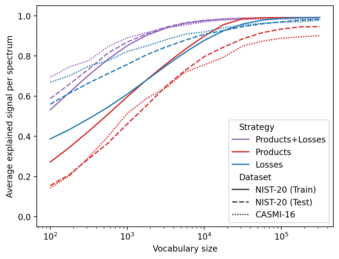
Figure 2 demonstrates the fraction of ion counts explained in the average mass spectrum as the training vocabulary size is varied. This shows most signal lies within peaks explainable by a relatively small number of product ion and neutral loss formulas. In particular, the vocabulary we use (of size $K=10^{4}$) is sufficient to explain $98\%$ of ion counts in the NIST-20 training split, which comprises 193,577 unique product ion formulas and 348,692 unique neutral loss formulas. We observe that a fixed vocabulary generalizes beyond NIST-20 to a separate dataset CASMI-16, indicating ‘formula sparsity’ is a general property of small molecule mass spectra and not limited to our particular training set. We also compare alternative strategies of picking only the top products or top losses: using both types of formulas explains more signal for a given $K$ than either alone.

6.2 GrAFF-MS outperforms bond-breaking and mass-binning on standard MS/MS datasets

Table 1 shows GrAFF-MS produces spectra with greater cosine similarity to ground-truth than either baseline. More of our spectra also meet the $C_{S\hat{S}}>0.7$ threshold for useful predictions. These results hold both for the NIST-20 test split and the independent test set CASMI-16. We see all methods perform better on CASMI-16 than NIST-20: this is because NIST-20 includes a minority of substantially larger molecules (max weight $986$Da) than CASMI-16 (max weight $539$Da), with which all three methods struggle.

Table 1: Mean cosine similarity $\mathbb{E}[C]$ and fraction of useful predictions $\mathbb{P}(C>0.7)$ on the NIST-20 test split and CASMI-16. $95\%$ confidence intervals are computed via nonparametric bootstrap.

	NIST-20 Test (N = 4548)		CASMI-16 (N = 156)
Method	$\mathbb{E}[C]$	$\mathbb{P}(C{>}0.7)$	$\mathbb{E}[C]$	$\mathbb{P}(C{>}0.7)$
CFM-ID	.52$\pm$.01	.35$\pm$.02	.75$\pm$.05	.70$\pm$.07
NEIMS	.60$\pm$.01	.50$\pm$.01	.63$\pm$.05	.54$\pm$.08
GrAFF-MS	.70$\pm$.01	.62$\pm$.02	.79$\pm$.05	.76$\pm$.07

6.3 Representing peaks as formulas scales better with molecular weight than bond-breaking

Figure 3: Empirical time complexity on NIST-20 structures with respect to molecular weight. Each dot is a structure. Solid lines are quadratic (blue) and linear (red) fits; dotted line indicates an average over all spectra computed using shuffled minibatches.

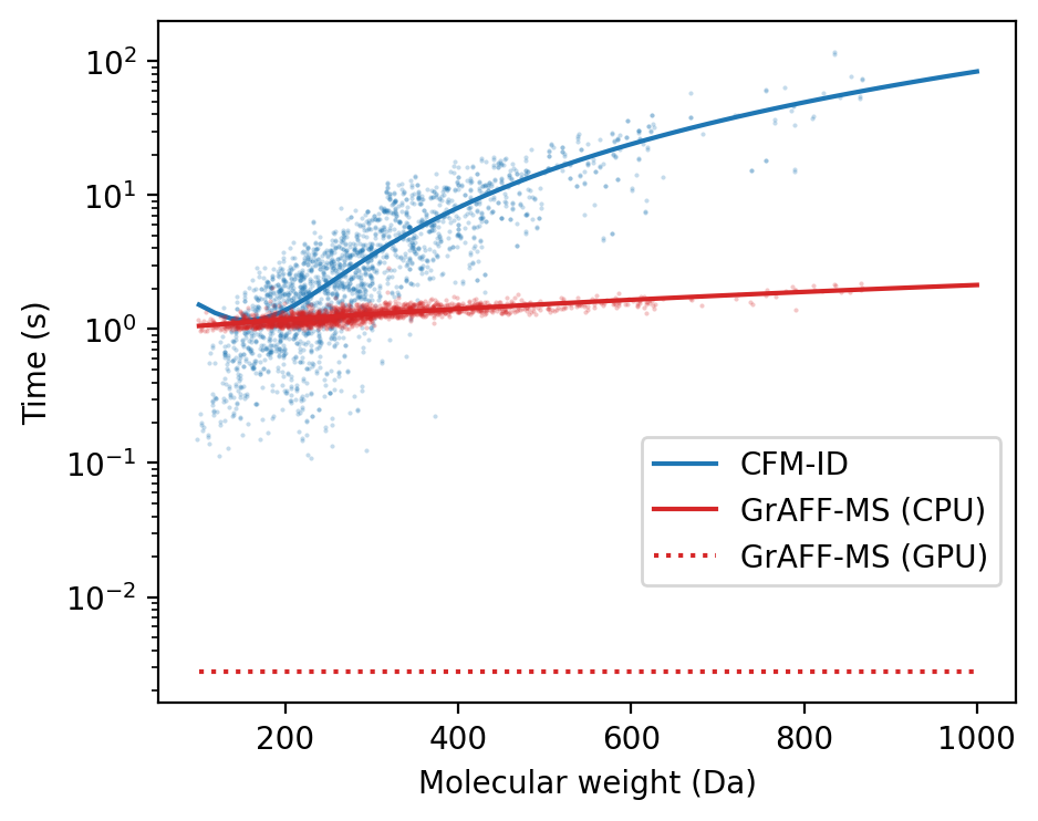
Figure 3 shows our approach to modelling high resolution spectra scales better with input size than bond-breaking. CFM-ID takes on average 4.9 seconds per structure in the NIST-20 test split, and scales quadratically $(R^{2}=0.78)$ with input size. (We believe this is because larger molecules in NIST-20 tend to be approximately path graphs – e.g. long hydrocarbon chains – with only quadratically many connected subgraphs.) In comparison, running GrAFF-MS on the CPU takes 1.3 core-seconds per spectrum, and scales approximately linearly $(R^{2}=0.65)$. This pays off at larger molecular weight: for molecules $>500$Da, our model is $16\times$ faster on average. Realistically, large-scale prediction will use the GPU: on a single GPU with batch size 512, predicting all of the NIST-20 test spectra averages to 2.8ms per spectrum (mostly spent in preprocessing on the CPU).

We can additionally estimate the time required for each approach to generate a reference library from all 2,259,751 structures below 1000Da in ChEMBL v3.1. Correcting for greater mean molecular weight in ChEMBL (405Da vs 292Da), this would take 2 hours running our PyTorch research code as-is on a single GPU. The same library would take 4 days to generate with 64 parallel instances of CFM-ID, which is written in optimized C++ code – showing the importance of efficiently representing the output space.

6.4 GrAFF-MS distinguishes very similar compounds and makes human-like mistakes

Figure 4: Three compounds from CASMI-16, with spectra predicted by our model (blue) against negated ground-truth (orange). Oxygens are shaded red by convention.

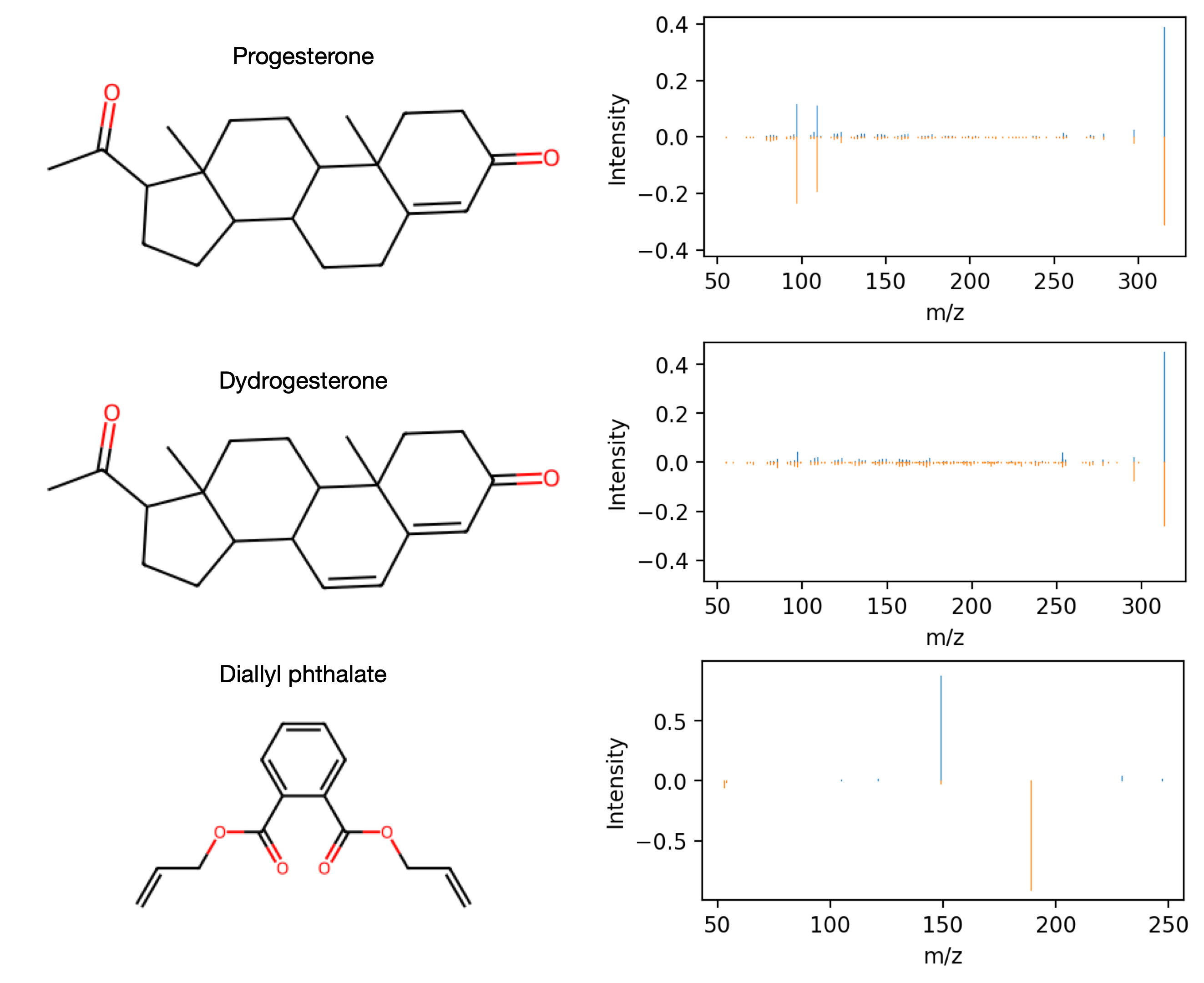
In Figure 4 we show some particularly challenging examples of mass spectra. The top and middle panels show two structurally similar compounds, differing only by the order of a carbon-carbon bond. Our approach correctly predicts distinct spectra for each ($C_{S\hat{S}}=0.98$, top; $C_{S\hat{S}}=0.95$, middle). The third molecule is an example where we fail to predict a realistic spectrum ($C_{S\hat{S}}=0.03$), but in a manner in which a human expert would also fail. This molecule is a member of the phthalate class, which chemists recognize by a characteristic dominant peak at 149Da [41]. Our model predicts this same peak, correctly recognizing a phthalate: but in this case that peak is relatively minor, indicating atypical fragmentation chemistry.

7 Discussion

In this work we develop GrAFF-MS, a graph neural network for predicting high resolution mass spectra of small molecules. Unlike previous approaches that force a tradeoff between $m/z$ resolution and a tractable learning problem, GrAFF-MS is both computationally efficient and capable of modelling the high-resolution $m/z$ information essential to mass spectrometry. This is made possible by our discovery that mass spectra of small molecules can be closely approximated as distributions over a fixed vocabulary of molecular formulas, highlighting the value that domain-aware modelling can add to molecular machine learning. Particularly surprising was that we outperform CFM-ID, which trades model expressivity for an even stronger scientific prior that we expected would contribute to better generalization. However, this prior incurs a heavy cost in time complexity, making it impractical to train CFM-ID on hundreds of thousands of spectra as we did.

Future directions include pretraining on large-scale property prediction tasks, revisiting sequential formula decoding, and incorporating additional scientific priors about fragmentation chemistry. Overall we anticipate this work will both accelerate scientific discovery and demonstrate mass spectrometry to be a compelling domain for continued machine learning research.

Appendix A Fixed vocabulary selection

Algorithm 1 describes our procedure for selecting the product ions $\hat{\mathcal{P}}$ and neutral losses $\hat{\mathcal{L}}$. We use the shorthand $\mathcal{F}^{n}_{i}=\mathcal{F}(P_{n},m_{i},\epsilon)$ to indicate the set of formulas computed by mass decomposition. When mass decomposition yields more than one formula annotation for a peak, here we split the peak height uniformly among all annotations.

Algorithm 1 Fixed vocabulary selection

  Input: training spectra and precursors $\{(S_{n},P_{n})\}_{n=1}^{N}$, vocabulary size $K$, tolerance $\epsilon$

  Initialize $F_{f}=0,L_{l}=0,\hat{\mathcal{P}}=\emptyset,\hat{\mathcal{L}}=\emptyset$

  for $n=1\dots N$ do

     for $(m_{i},y_{i})\in S_{n}$ do

        for $f\in\mathcal{F}^{n}_{i}$ do

           $l=P_{n}-f$

           $F_{f}=F_{f}+y_{i}/|\mathcal{F}^{n}_{i}|$

           $L_{l}=L_{l}+y_{i}/|\mathcal{F}^{n}_{i}|$

        end for

     end for

  end for

  Sort $F$ and $L$

  while $|\hat{\mathcal{P}}|+|\hat{\mathcal{L}}|\leq K$ do

     $f=$ first element of $F$

     $l=$ first element of $L$

     if $F_{f}>L_{l}$ then

        Add $f$ to $\hat{\mathcal{P}}$

        Remove $f$ from $F$

     else

        Add $l$ to $\hat{\mathcal{L}}$

        Remove $l$ from $L$

     end if

  end while

Appendix B Derivation of peak-marginal cross entropy

We derive our loss function from physical first principles, making a number of minor modelling assumptions:

• The number of precursor ions accumulated by the instrument is Poisson with rate $\lambda$.

• Each individual precursor ion is independently converted into fragment $f$ with probability $p_{f}$.

• The instrument resolution parameter $\epsilon$ is sufficiently small that separate peaks do not overlap: there exists exactly one peak $i(f)$ for every $f:p_{f}>0$ satisfying $|\langle\mu,f\rangle-m_{i}|\leq\epsilon m_{i}$.

By the splitting property, the number of ions of each fragment are independently Poisson with rate $\lambda_{f}=\lambda p_{f}$. By the merging property, the height of peak $i$ is also a Poisson r.v. $K_{i}$ with rate $\lambda_{i}=\sum_{f\in\mathcal{F}_{i}}\lambda_{f}$, where $\mathcal{F}_{i}$ denotes the set of fragments whose theoretical masses all fall within the measurement error $\epsilon m_{i}$ of peak $i$.

The log-likelihood for the peak height is (taking equality up to constants $C$ w.r.t. $p_{f}$):

$$\log P(K_{i}=k_{i})$$ (23)

$$= \ k_{i}\log\lambda_{i}-\lambda_{i}-\log k_{i}!$$ (24)

$$= \ k_{i}\log\left(\sum_{f\in\mathcal{F}_{i}}\lambda_{f}\right)-\left(\sum_{f\in\mathcal{F}_{i}}\lambda_{f}\right)+C$$ (25)

$$= \ k_{i}\log\left(\sum_{f\in\mathcal{F}_{i}}\lambda p_{f}\right)-\left(\sum_{f\in\mathcal{F}_{i}}\lambda p_{f}\right)$$ (26)

$$= \ k_{i}\log\lambda+k_{i}\log\left(\sum_{f\in\mathcal{F}_{i}}p_{f}\right)-\lambda\sum_{f\in\mathcal{F}_{i}}p_{f}$$ (27)

$$= \ C+k_{i}\log\left(\sum_{f\in\mathcal{F}_{i}}p_{f}\right)-\lambda\sum_{f\in\mathcal{F}_{i}}p_{f}$$ (28)

where (25) uses merging, and (26) uses splitting. Because each fragment is assigned to exactly one peak (no overlap), the peak heights $\{K_{i}:i\in S\}$ are independent. Let the total number of accumulated ions $K=\sum_{i\in S}k_{i}$ in spectrum $S$. Defining $y_{i}=k_{i}/K$:

$$\log P(\{K_{i}=k_{i}:i\in S\})$$ (29)

$$= \sum_{i\in S}\log P(K_{i}=k_{i})$$ (30)

$$= \ \sum_{i\in S}\left(k_{i}\log\left(\sum_{f\in\mathcal{F}_{i}}p_{f}\right)-\lambda\sum_{f\in\mathcal{F}_{i}}p_{f}\right)$$ (31)

$$= \ \sum_{i\in S}(Ky_{i})\log\left(\sum_{f\in\mathcal{F}_{i}}p_{f}\right)-\lambda\sum_{i\in S}\sum_{f\in\mathcal{F}_{i}}p_{f}$$ (32)

$$= \ K\sum_{i\in S}y_{i}\log\left(\sum_{f\in\mathcal{F}_{i}}p_{f}\right)-\lambda\cdot 1$$ (33)

$$= \ C\sum_{i\in S}y_{i}\log\left(\sum_{f\in\mathcal{F}_{i}}p_{f}\right)+C^{\prime}$$ (34)

where (33) again uses our assumption that every fragment is assigned to exactly one peak. Dropping the constants and negating the final term yields the peak-marginal cross-entropy loss for a single spectrum. ∎

Appendix C Model hyperparameters

We use a vocabulary of $K=10000$ formulas. We train an $L=6$-layer encoder and $L^{\prime}=2$-layer decoder with $d_{enc}=512$ and $d_{dec}=1024$, resulting in $44.6$ million trainable parameters. We use the $d_{eig}=8$ lowest-frequency eigenvalues, truncating or padding with zeros. All dropout is applied at rate $0.1$. We use a batch size of $512$ and the Adam optimizer [42] with learning rate $5\times 10^{-4}$. We train for 100 epochs and use the model from the epoch with the lowest validation loss. All models are trained using PyTorch Lightning with automatic mixed precision on 2 Tesla V100 GPUs.

Appendix D Mass spectral covariates

Table 2: Mass spectral covariates used in our model.

Feature	Range	Comment
Normalized collision energy	$[0,200]$	Thermo Scientific PSB104, “Normalized Collision Energy Technology”
Precursor type	$[M+H]^{+}$, $[M-H]^{-}$	Includes ionization mode $\&$ adduct composition
Instrument model	Orbitrap Fusion Lumos, Thermo Finnigan Elite Orbitrap, Thermo Finnigan Velos Orbitrap	Different limits of detection
Has isotopic peaks	False, True	Proxy for width setting of precursor mass filter

References

- [1] Katja Dettmer, Pavel A. Aronov, and Bruce D. Hammock. Mass spectrometry-based metabolomics. Mass Spectrometry Reviews, 26(1):51–78, August 2006.
- [2] Atanas G Atanasov, Sergey B Zotchev, Verena M Dirsch, and Claudiu T Supuran. Natural products in drug discovery: advances and opportunities. Nature reviews Drug discovery, 20(3):200–216, 2021.
- [3] Ethan D. Evans, Claire Duvallet, Nathaniel D. Chu, Michael K. Oberst, Michael A. Murphy, Isaac Rockafellow, David Sontag, and Eric J. Alm. Predicting human health from biofluid-based metabolomics using machine learning. Scientific Reports, 10(1), October 2020.
- [4] Hilary M. Brown, Trevor J. McDaniel, Patrick W. Fedick, and Christopher C. Mulligan. The current role of mass spectrometry in forensics and future prospects. Analytical Methods, 12(32):3974–3997, 2020.
- [5] F. Hernández, J. V. Sancho, M. Ibáñez, E. Abad, T. Portolés, and L. Mattioli. Current use of high-resolution mass spectrometry in the environmental sciences. Analytical and Bioanalytical Chemistry, 403(5):1251–1264, February 2012.
- [6] Ricardo R da Silva, Pieter C Dorrestein, and Robert A Quinn. Illuminating the dark matter in metabolomics. Proceedings of the National Academy of Sciences, 112(41):12549–12550, 2015.
- [7] Oliver Fiehn. Critical Assessment of Small Molecule Identification 2022. http://www.casmi-contest.org/2022/index.shtml/, 2022. [Online; accessed 12-December-2022].
- [8] Stephen Stein. Mass spectral reference libraries: An ever-expanding resource for chemical identification. Analytical Chemistry, 84(17):7274–7282, July 2012.
- [9] Christoph A Krettler and Gerhard G Thallinger. A map of mass spectrometry-based in-silico fragmentation prediction and compound identification in metabolomics. Briefings in Bioinformatics, 22(6), March 2021.
- [10] Jennifer N. Wei, David Belanger, Ryan P. Adams, and D. Sculley. Rapid prediction of electron–ionization mass spectrometry using neural networks. ACS Central Science, 5(4):700–708, March 2019.
- [11] Hao Zhu, Liping Liu, and Soha Hassoun. Using graph neural networks for mass spectrometry prediction, 2020.
- [12] Adamo Young, Bo Wang, and Hannes Röst. Massformer: Tandem mass spectrum prediction with graph transformers, 2021.
- [13] Fei Wang, Jaanus Liigand, Siyang Tian, David Arndt, Russell Greiner, and David S. Wishart. CFM-ID 4.0: More accurate ESI-MS/MS spectral prediction and compound identification. Analytical Chemistry, 93(34):11692–11700, August 2021.
- [14] Christoph Ruttkies, Steffen Neumann, and Stefan Posch. Improving MetFrag with statistical learning of fragment annotations. BMC Bioinformatics, 20(1), July 2019.
- [15] Robert K. Lindsay, Bruce G. Buchanan, Edward A. Feigenbaum, and Joshua Lederberg. DENDRAL: A case study of the first expert system for scientific hypothesis formation. Artificial Intelligence, 61(2):209–261, June 1993.
- [16] Kai Dührkop, Marcus Ludwig, Marvin Meusel, and Sebastian Böcker. Faster mass decomposition. In Lecture Notes in Computer Science, pages 45–58. Springer Berlin Heidelberg, 2013.
- [17] Tobias Kind and Oliver Fiehn. Seven golden rules for heuristic filtering of molecular formulas obtained by accurate mass spectrometry. BMC Bioinformatics, 8(1), March 2007.
- [18] Liu Cao, Mustafa Guler, Azat Tagirdzhanov, Yi-Yuan Lee, Alexey Gurevich, and Hosein Mohimani. Moldiscovery: learning mass spectrometry fragmentation of small molecules. Nature Communications, 12(1):1–13, 2021.
- [19] Anna Gaulton, Anne Hersey, Michał Nowotka, A. Patrícia Bento, Jon Chambers, David Mendez, Prudence Mutowo, Francis Atkinson, Louisa J. Bellis, Elena Cibrián-Uhalte, Mark Davies, Nathan Dedman, Anneli Karlsson, María Paula Magariños, John P. Overington, George Papadatos, Ines Smit, and Andrew R. Leach. The ChEMBL database in 2017. Nucleic Acids Research, 45(D1):D945–D954, November 2016.
- [20] F. W. McLafferty. Mass spectrometric analysis. molecular rearrangements. Analytical Chemistry, 31(1):82–87, January 1959.
- [21] Jeroen Koopman and Stefan Grimme. From QCEIMS to QCxMS: A tool to routinely calculate CID mass spectra using molecular dynamics. Journal of the American Society for Mass Spectrometry, 32(7):1735–1751, June 2021.
- [22] Xie-Xuan Zhou, Wen-Feng Zeng, Hao Chi, Chunjie Luo, Chao Liu, Jianfeng Zhan, Si-Min He, and Zhifei Zhang. pDeep: Predicting MS/MS spectra of peptides with deep learning. Analytical Chemistry, 89(23):12690–12697, November 2017.
- [23] Siegfried Gessulat, Tobias Schmidt, Daniel Paul Zolg, Patroklos Samaras, Karsten Schnatbaum, Johannes Zerweck, Tobias Knaute, Julia Rechenberger, Bernard Delanghe, Andreas Huhmer, Ulf Reimer, Hans-Christian Ehrlich, Stephan Aiche, Bernhard Kuster, and Mathias Wilhelm. Prosit: proteome-wide prediction of peptide tandem mass spectra by deep learning. Nature Methods, 16(6):509–518, May 2019.
- [24] Keyulu Xu, Weihua Hu, Jure Leskovec, and Stefanie Jegelka. How powerful are graph neural networks? In 7th International Conference on Learning Representations, ICLR 2019, New Orleans, LA, USA, May 6-9, 2019. OpenReview.net, 2019.
- [25] Weihua Hu, Bowen Liu, Joseph Gomes, Marinka Zitnik, Percy Liang, Vijay Pande, and Jure Leskovec. Strategies for pre-training graph neural networks. In International Conference on Learning Representations, 2020.
- [26] Derek Lim, Joshua Robinson, Lingxiao Zhao, Tess Smidt, Suvrit Sra, Haggai Maron, and Stefanie Jegelka. Sign and basis invariant networks for spectral graph representation learning, 2022.
- [27] Justin Gilmer, Samuel S. Schoenholz, Patrick F. Riley, Oriol Vinyals, and George E. Dahl. Neural message passing for quantum chemistry. In Doina Precup and Yee Whye Teh, editors, Proceedings of the 34th International Conference on Machine Learning, ICML 2017, Sydney, NSW, Australia, 6-11 August 2017, volume 70 of Proceedings of Machine Learning Research, pages 1263–1272. PMLR, 2017.
- [28] Mufei Li, Jinjing Zhou, Jiajing Hu, Wenxuan Fan, Yangkang Zhang, Yaxin Gu, and George Karypis. Dgl-lifesci: An open-source toolkit for deep learning on graphs in life science. ACS Omega, 2021.
- [29] Matthias Fey and Jan E. Lenssen. Fast graph representation learning with PyTorch Geometric. In ICLR Workshop on Representation Learning on Graphs and Manifolds, 2019.
- [30] Tianle Cai, Shengjie Luo, Keyulu Xu, Di He, Tie-Yan Liu, and Liwei Wang. Graphnorm: A principled approach to accelerating graph neural network training. In Marina Meila and Tong Zhang, editors, Proceedings of the 38th International Conference on Machine Learning, ICML 2021, 18-24 July 2021, Virtual Event, volume 139 of Proceedings of Machine Learning Research, pages 1204–1215. PMLR, 2021.
- [31] Meng Joo Er, Yong Zhang, Ning Wang, and Mahardhika Pratama. Attention pooling-based convolutional neural network for sentence modelling. Information Sciences, 373:388–403, December 2016.
- [32] National Institute of Standards and Technology. Nist-20, 2020.
- [33] Kai Dührkop. Deep kernel learning improves molecular fingerprint prediction from tandem mass spectra. Bioinformatics, 38(Supplement_1):i342–i349, June 2022.
- [34] Stephen R Heller, Alan McNaught, Igor Pletnev, Stephen Stein, and Dmitrii Tchekhovskoi. InChI, the IUPAC international chemical identifier. Journal of Cheminformatics, 7(1), May 2015.
- [35] Zhenqin Wu, Bharath Ramsundar, Evan N. Feinberg, Joseph Gomes, Caleb Geniesse, Aneesh S. Pappu, Karl Leswing, and Vijay Pande. MoleculeNet: a benchmark for molecular machine learning. Chemical Science, 9(2):513–530, 2018.
- [36] Emma L. Schymanski, Christoph Ruttkies, Martin Krauss, Céline Brouard, Tobias Kind, Kai Dührkop, Felicity Allen, Arpana Vaniya, Dries Verdegem, Sebastian Böcker, Juho Rousu, Huibin Shen, Hiroshi Tsugawa, Tanvir Sajed, Oliver Fiehn, Bart Ghesquière, and Steffen Neumann. Critical assessment of small molecule identification 2016: automated methods. Journal of Cheminformatics, 9(1), March 2017.
- [37] Carlos Guijas, J. Rafael Montenegro-Burke, Xavier Domingo-Almenara, Amelia Palermo, Benedikt Warth, Gerrit Hermann, Gunda Koellensperger, Tao Huan, Winnie Uritboonthai, Aries E. Aisporna, Dennis W. Wolan, Mary E. Spilker, H. Paul Benton, and Gary Siuzdak. METLIN: A technology platform for identifying knowns and unknowns. Analytical Chemistry, 90(5):3156–3164, January 2018.
- [38] Maria Lorna A. De Leoz, Yamil Simón-Manso, Robert J. Woods, and Stephen E. Stein. Cross-ring fragmentation patterns in the tandem mass spectra of underivatized sialylated oligosaccharides and their special suitability for spectrum library searching. Journal of the American Society for Mass Spectrometry, 30(3):426–438, December 2018.
- [39] Wout Bittremieux, Robin Schmid, Florian Huber, Justin J. J. van der Hooft, Mingxun Wang, and Pieter C. Dorrestein. Comparison of cosine, modified cosine, and neutral loss based spectrum alignment for discovery of structurally related molecules. Journal of the American Society for Mass Spectrometry, 33(9):1733–1744, August 2022.
- [40] Gert Wohlgemuth, Sajjan S Mehta, Ramon F Mejia, Steffen Neumann, Diego Pedrosa, Tomáš Pluskal, Emma L Schymanski, Egon L Willighagen, Michael Wilson, David S Wishart, Masanori Arita, Pieter C Dorrestein, Nuno Bandeira, Mingxun Wang, Tobias Schulze, Reza M Salek, Christoph Steinbeck, Venkata Chandrasekhar Nainala, Robert Mistrik, Takaaki Nishioka, and Oliver Fiehn. SPLASH, a hashed identifier for mass spectra. Nature Biotechnology, 34(11):1099–1101, November 2016.
- [41] Yassin A. Jeilani, Beatriz H. Cardelino, and Victor M. Ibeanusi. Density functional theory and mass spectrometry of phthalate fragmentations mechanisms: Modeling hyperconjugated carbocation and radical cation complexes with neutral molecules. Journal of the American Society for Mass Spectrometry, 22(11), August 2011.
- [42] Diederik P Kingma and Jimmy Ba. Adam: A method for stochastic optimization. 2015.