DBGDGM: Dynamic Brain Graph Deep Generative Model

Abstract

Graphs are a natural representation of brain activity derived from functional magnetic imaging (fMRI) data. It is well known that clusters of anatomical brain regions, known as functional connectivity networks (FCNs), encode temporal relationships which can serve as useful biomarkers for understanding brain function and dysfunction. Previous works, however, ignore the temporal dynamics of the brain and focus on static graphs. In this paper, we propose a dynamic brain graph deep generative model (DBGDGM) which simultaneously clusters brain regions into temporally evolving communities and learns dynamic unsupervised node embeddings. Specifically, DBGDGM represents brain graph nodes as embeddings sampled from a distribution over communities that evolve over time. We parameterise this community distribution using neural networks that learn from subject and node embeddings as well as past community assignments. Experiments demonstrate DBGDGM outperforms baselines in graph generation, dynamic link prediction, and is comparable for graph classification. Finally, an analysis of the learnt community distributions reveals overlap with known FCNs reported in neuroscience literature.

1 Introduction

Functional magnetic resonance imaging (fMRI) is a non-invasive imaging technique primarily used to measure blood-oxygen level dependent (BOLD) signal in the brain [huettel2004functional]. A natural representation of fMRI data is as a discrete-time graph, henceforth referred to as a dynamic brain graph (DBG), consisting of a set of fixed nodes corresponding to anatomically separated brain regions and a set of time-varying edges determined by a measure of dynamic functional connectivity (dFC) (calhoun2014chronnectome). DBGs have been widely used in graph-based network analysis for understanding brain function (hirsch2022graph; raz2016functional) and dysfunction (alonso2020dynamics; dautricourt2022dynamic; qingbao2015dynamic).

Recently, there is growing interest in using deep learning-based methods for learning representations of graph-structured data (goyal2018graph; hamilton2020graph). A graph representation typically consists of a low-dimensional vector embedding of either the entire graph (narayanan2017graph2vec) or a part of it’s structure such as nodes (grover2016node2vec), edges (gao2019edge2vec), or sub-graphs (adhikari2017distributed). Although originally formulated for static graphs (i.e. not time-varying), several existing methods have been extended (mahdavi2018dynnode2vec; goyal2020dyngraph2vec), and new ones proposed (zhou2018dynamic; sankar2020dysat), for dynamic graphs. The embeddings are usually learnt in either a supervised or unsupervised fashion and typically used in tasks such as node classification (pareja2020evolvegcn) and dynamic link prediction (goyal2018dyngem).

To date, very few deep learning-based methods have been designed for, or existing methods applied to, representation learning of DBGs. Those that do, tend to use graph neural networks (GNNs) that are designed for learning node- and graph-level embeddings for use in graph classification (kim2021learning; dahan2021improving). Although node/graph-level embeddings are effective at representing local/global graph structure, they are less adept at representing topological structures in-between these two extremes such a clusters of nodes or communities (wang2017community). Recent methods that explicitly incorporate community embeddings alongside node embeddings have shown improved performance for static graph representation learning tasks (sun2019vgraph; cavallari2017learning). How to leverage the relatedness of graph, node, and community embeddings in a unified framework for DBG representation learning remains under-explored. We refer to Appendix LABEL:appendix_related_work for a summary of related work.

Contributions

To address these shortcomings, we propose DBGDGM, a hierarchical deep generative model (DGM) designed for unsupervised representing learning on DBGs derived from multi-subject fMRI data. Specifically, DBGDGM represents nodes as embeddings sampled from a distribution over communities that evolve over time. The community distribution is parameterized using neural networks (NNs) that learn from graph and node embeddings as well as past community assignments. We evaluate DBGDGM on multiple real-world fMRI datasets and show that it outperforms state-of-the-art baselines for graph reconstruction, dynamic link prediction, and achieves comparable results for graph classification.

2 Problem formulation

We consider a dataset of multi-subject DBGs derived from fMRI data $\mathcal{D}\equiv\mathcal{G}^{(1:S,\,1:T)}=\{\mathcal{G}^{(s,\,t)}\}_{s,\,t=1}^{S,\,T}$ that share a common set of nodes $\mathcal{V}=\{v_{1},\,\dots,\,v_{N}\}$ over $T\in\mathbb{N}$ timepoints for $S\in\mathbb{N}$ subjects. Each $\mathcal{G}^{(s,\,t)}\in\mathcal{G}^{(1:S,\,1:T)}$ denotes a non-attributed, unweighted, and undirected brain graph snapshot for the $s$-th subject at the $t$-th timepoint. We define a brain graph snapshot as a tuple $\mathcal{G}^{(s,\,t)}=(\mathcal{V},\mathcal{E}^{(s,\,t)})$ where $\mathcal{E}^{(s,\,t)}\subseteq\mathcal{V}\times\mathcal{V}$ denotes an edge set. The $i$-th edge for the $s$-th subject at the $t$-th timepoint $e^{(s,\,t)}_{i}\in\mathcal{E}^{(s,\,t)}$ is defined $e^{(s,\,t)}_{i}=(w^{(s,t)}_{i},\,c^{(s,t)}_{i})$ where $w^{(s,t)}_{i}$ is a source node and $c^{(s,t)}_{i}$ is a target node. We assume each node corresponds to a brain region making the number of nodes $|\mathcal{V}|=V\in\mathbb{N}$ fixed over subjects and time. We also assume edges correspond to a measure of dFC allowing the number of edges $|\mathcal{E}^{(s,\,t)}|=E^{(s,\,t)}\in\mathbb{N}$ vary over subjects and time. We further assume there exists $K\in\mathbb{N}$ clusters of nodes, or communities, the membership of which dynamically changes over time for each subject. Let $z^{(s,\,t)}_{i}\in[1:K]$ denote the latent community assignment of the $i$-th edge for the $s$-th subject at the $t$-th timepoint. For each subject’s DBG our aim is to learn, in an unsupervised fashion, graph $\bm{\alpha}^{(s)}\in\mathbb{R}^{H_{\alpha}}$, node $\bm{\phi}_{1:N}^{(s,\,t)}=[\bm{\phi}_{n}^{(s,\,t)}]\in\mathbb{R}^{N\times H_{\phi}}$, and community $\bm{\psi}_{1:K}^{(s,\,t)}=[\bm{\psi}_{k}^{(s,\,t)}]\in\mathbb{R}^{K\times H_{\psi}}$ representations of dimensions $H_{\alpha}$, $H_{\phi}$, $H_{\psi}\in\mathbb{N}$, respectively, for use in a variety of downstream tasks.

3 Method

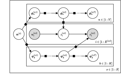
Figure 1: Plate diagram for DBGDGM. Latent and observed variables are denoted by white-and gray-shaded circles, respectively. Solid black squares denote non-linear mappings parameterized by NNs.

DBGDGM defines a hierarchical deep generative model and inference network for the end-to-end learning of graph, node, and community embeddings from multi-subject DBG data. Specifically, DBGDGM treats the embeddings and edge community assignments as latent random variables collectively denoted $\Omega^{(s,\,t)}=\{\bm{\alpha}^{(s)},\,$ $\bm{\phi}^{(s,\,t)}_{1:N},\,$ $\bm{\psi}^{(s,\,t)}_{1:K},\{z_{i}^{(s,\,t)}\}_{i=1}^{E^{(s,\,t)}}\}$, which along with the observed DBGs, defines a probabilistic latent variable model with joint density $p_{\theta}(\mathcal{G}^{1:S,\,1:T},\Omega^{1:S,\,1:T})$.

3.1 Generative model

Graph embeddings

We begin the generative process by sampling graph embeddings from a prior $\bm{\alpha}^{(s)}\sim p_{\theta_{\alpha}}(\bm{\alpha}^{(s)})$ implemented as a normal distribution following

$$p_{\theta_{\alpha}}(\bm{\alpha}^{(s)})=\text{Normal}(\bm{0}_{H_{\alpha}},\,\mathbf{I}_{H_{\alpha}})$$ (1)

where $\bm{0}_{H_{\alpha}}$ is a matrix of zeros and $\mathbf{I}_{H_{\alpha}}$ is a identity matrix. Each embedding is a vector $\bm{\alpha}^{(s)}\in\mathbb{R}^{H_{\alpha}}$ representing subject-specific information that remains fixed over time.

Node and community embeddings

Next, let $\bm{\phi}_{n}^{(s,\,t)}\in\mathbb{R}^{H_{\phi}}$ and $\bm{\psi}_{k}^{(s,\,t)}\in\mathbb{R}^{H_{\psi}}$ denote the $n$-th node and the $k$-th community embedding, respectively. To incorporate temporal dynamics, we assume node and community embeddings are related through Markov chains with prior transition distributions $\bm{\phi}_{n}^{(s,\,t)}\sim p_{\theta_{\phi}}(\bm{\phi}^{(s,\,t)}_{n}|\bm{\phi}^{(s,\,t-1)}_{n},\,\bm{\alpha}^{(s)})$ and $\bm{\psi}_{k}^{(s,\,t)}\sim p_{\theta_{\psi}}(\bm{\psi}^{(s,\,t)}_{k}|\bm{\psi}^{(s,\,t-1)}_{k},\,\bm{\alpha}^{(s)})$. We specify each prior to be a normal distribution following

$$p_{\theta_{\phi}}(\boldsymbol{\phi}^{(s,\,t)}_{n}|\boldsymbol{\phi}^{(s,\,t-1)}_{n},\,\boldsymbol{\alpha}^{(s)}) =\text{Normal}(\boldsymbol{\phi}^{(s,\,t-1)}_{n},\,\sigma_{\phi}\mathbf{I}_{H_{\phi}})$$ (2)

$$p_{\theta_{\psi}}(\boldsymbol{\psi}^{(s,\,t)}_{k}|\boldsymbol{\psi}^{(s,\,t-1)}_{k},\,\boldsymbol{\alpha}^{(s)}) =\text{Normal}(\boldsymbol{\psi}^{(s,\,t-1)}_{k},\,\sigma_{\psi}\mathbf{I}_{H_{\psi}})$$ (3)

where the graph embeddings are used for initializing the means, i.e., $\bm{\phi}_{n}^{(s,\,0)}=\bm{\alpha}^{(s)}$, $\bm{\psi}_{k}^{(s,\,0)}=\bm{\alpha}^{(s)}$ and the standard deviations $\sigma_{\phi},\sigma_{\psi}\in\mathbb{R}_{>0}$ are hyperparameters controlling how smoothly each embedding changes between consecutive timepoints.

Edge generation

We next describe the edge generative process of a graph snapshot $\mathcal{G}^{(s,\,t)}\in\mathcal{G}^{(1:S,\,1:T)}$. Similar to sun2019vgraph, for each edge $e^{(s,\,t)}_{i}=(w^{(s,\,t)}_{i},\,c^{(s,\,t)}_{i})\in\mathcal{E}^{(s,\,t)}$ we first sample a latent community assignment $z_{i}^{(s,\,t)}\in[1:K]$ from a conditional prior $z_{i}^{(s,\,t)}\sim p_{\theta_{z}}(z_{i}^{(s,\,t)}|w_{i}^{(s,\,t)})$ implemented as a categorical distribution

$$\split p_{\theta_{z}}(z_{i}^{(s,\,t)}|w_{i}^{(s,\,t)})=\text{Categorical}(\bm{\pi}_{\theta_{z}}^{(s,\,t)}),\quad\bm{\pi}_{\theta_{z}}^{(s,\,t)}=\text{MLP}_{\theta_{z}}(\bm{\phi}_{w_{i}}^{(s,\,t)})$$ (4)

where $\text{MLP}_{\theta_{z}}:\mathbb{R}^{H_{\phi}}\rightarrow\mathbb{R}^{K}$ is a $L_{z}$-layered multilayered perception (MLP) that parameterizes community probabilities using node embeddings indexed by $w^{(s,\,t)}_{i}$. In other words, each source node $w^{(s,\,t)}_{i}$ is represented as a mixture of communities. A linked target node $c_{i}^{(s,\,t)}\in[1:N]$ is then sampled from the conditional likelihood $c_{i}^{(s,\,t)}\sim p_{\theta_{c}}(c_{i}^{(s,\,t)}|z_{i}^{(s,\,t)})$ which is also implemented as a categorical distribution

$$\split p_{\theta_{c}}(c_{i}^{(s,\,t)}|z_{i}^{(s,\,t)})=\text{Categorical}(\bm{\pi}_{\theta_{c}}^{(s,\,t)}),\quad\bm{\pi}_{\theta_{c}}^{(s,\,t)}=\text{MLP}_{\theta_{c}}(\bm{\psi}_{z_{i}}^{(s,\,t)})$$ (5)

where $\text{MLP}_{\theta_{c}}:\mathbb{R}^{H_{\psi}}\rightarrow\mathbb{R}^{N}$ is a $L_{c}$-layered MLP that parameterizes node probabilities using community embeddings indexed by $z_{i}^{(s,\,t)}$. That is, each community assignment $z_{i}^{(s,\,t)}$ is represented as a mixture of nodes. By integrating out the latent community assignment variable

$$p(c^{(s,\,t)}_{i}|w^{(s,\,t)}_{i})=\sum_{z^{(s,\,t)}_{i}\in[1:K]}p_{\theta_{c}}(c_{i}^{(s,\,t)}|z_{i}^{(s,\,t)})p_{\theta_{z}}(z_{i}^{(s,\,t)}|w_{i}^{(s,\,t)})$$ (6)

we define the likelihood of node $c^{(s,\,t)}_{i}$ being a linked neighbor of node $w^{(s,\,t)}_{i}$, in a given graph snapshot.

Factorized generative model

Given this model specification, the joint probability of the observed data and the latent variables can be factorized following

$$\split p_{\theta}(\mathcal{G}^{1:S\,1:T},\,\Omega^{1:S,1:T})={}&\prod_{s=1}^{S}\Bigg{(}p_{\theta_{\alpha}}(\bm{\alpha}^{(s)})\prod_{t=1}^{T}\Bigg{(}\prod_{n=1}^{V}p_{\theta_{\phi}}(\bm{\phi}^{(s,\,t)}_{n}|\bm{\phi}^{(s,\,t-1)}_{n})\\ \prod_{k=1}^{K}p_{\theta_{\psi}}(\bm{\psi}^{(s,t)}_{k}|\bm{\psi}^{(s,t-1)}_{k})\\ \prod_{i=1}^{E^{(s,\,t)}}p_{\theta_{z}}(z_{i}^{(s,\,t)}|\bm{\phi}_{w_{i}}^{(s,\,t)})p_{\theta_{c}}(c^{(s,\,t)}_{i}|\bm{\psi}_{z_{i}}^{(s,\,t)})\Bigg{)}\Bigg{)}$$ (7)

where $\theta=\{\theta_{c}\,,\theta_{z}\}$ is the set of generative model parameters, i.e., NN weights. The generative model of DBGDGM summarized in Appendix LABEL:appendix_method

3.2 Inference network

To learn the embeddings, we must infer the posterior distribution over all latent variables conditioned on the observed data $p_{\theta}(\Omega^{(1:S,\,1:T)}|\mathcal{G}^{(1:S,\,1:T)})$. However, exact inference is intractable due the log marginal likelihood requiring integrals that are hard to evaluate, i.e., $\log p_{\theta}(\mathcal{G}^{(1:S,\,1:T)})=\int_{\Omega}\log p_{\theta}(\mathcal{G}^{(1:S,\,1:T)},\Omega^{(1:S,\,1:T)})d\Omega$. As a result, we use variational inference (jordan1999introduction) to approximate the true posterior with a variational distribution $q_{\lambda}(\Omega^{(1:S,1:T)})$ with parameters $\lambda$. To do this, we maximize a lower bound on the log marginal likelihood of the DBGs, referred to as the ELBO (evidence lower bound), defined as

$$\mathcal{L}_{\text{ELBO}}(\theta,\lambda)=\mathbb{E}_{q_{\lambda}}\Bigg{[}\log\frac{p_{\theta}(\mathcal{G}^{1:S,\,1:T},\,\Omega^{1:S,\,1:T})}{q_{\lambda}(\Omega^{(1:S,\,1:T)})}\Bigg{]}\leq\log p_{\theta}(\mathcal{G}^{(1:S,\,1:T)})$$ (8)

where $\mathbb{E}_{q_{\lambda}}[\cdot]$ denotes the expectation taken with respect to the variational distribution $q_{\lambda}(\Omega^{(1:S,\,1:T)})$. By maximizing the ELBO with respect to the generative and variational parameters $\theta$ and $\lambda$ we train our generative model and perform Bayesian inference, respectively.

Structured variational distribution

To ensure a good approximation to true posterior, we retain the Markov properties of the node and community embeddings. This results in a structured variational distribution (hoffman2015structured; saul1995exploiting) which factorizes following

$$\split q_{\lambda}(\Omega^{(1:S,\,1:T)})={}&\prod_{s=1}^{S}\Bigg{(}q_{\lambda_{\alpha}}(\bm{\alpha}^{(s)})\prod_{t=1}^{T}\Bigg{(}\prod_{n=1}^{V}q_{\lambda_{\phi}}(\bm{\phi}_{n}^{(s,\,t)}|\,\bm{\phi}_{n}^{(s,\,t-1)})\\ \prod_{k=1}^{K}q_{\lambda_{\psi}}(\bm{\psi}_{k}^{(s,\,t)}|\,\bm{\psi}_{k}^{(s,\,t-1)})\prod_{i=1}^{E^{(s,\,t)}}q_{\lambda_{z}}(z_{i}^{(s,\,t)}|\,\bm{\phi}_{w_{i}}^{(s,\,t)},\,\bm{\phi}_{c_{i}}^{(s,\,t)})\Bigg{)}\Bigg{)}$$ (9)

where each distribution is specified to mimic the structure of the generative model so that