Causal Bandits without Graph Learning

Abstract

We study the causal bandit problem when the causal graph is unknown and develop an efficient algorithm for finding the parent node of the reward node using atomic interventions. We derive the exact equation for the expected number of interventions performed by the algorithm and show that under certain graphical conditions it could perform either logarithmically fast or, under more general assumptions, slower but still sublinearly in the number of variables. We formally show that our algorithm is optimal as it meets the universal lower bound we establish for any algorithm that performs atomic interventions. Finally, we extend our algorithm to the case when the reward node has multiple parents. Using this algorithm together with a standard algorithm from bandit literature leads to improved regret bounds.

1 Introduction

Multi-armed bandit (MAB) settings provide a rich theoretical context for formalizing and analyzing sequential experimental design procedures. Each arm in a MAB setting represents an experiment/action and the consequence of pulling an arm is represented by a stochastic reward signal. The objective of a learner in a MAB problem is to select a sequence of arms over a time horizon in order to either find an arm that results in the maximum reward or to maximize the cumulative reward during this time horizon. Bandit problems have a growing list of applications in various domains such as marketing Huo and Fu (2017); Sawant et al. (2018), recommendation systems Heckel et al. (2019); Silva et al. (2022), clinical trials Liu et al. (2020), etc. MAB algorithms are designed for the setting when there is no structural relationships between different arms. However, this assumption is often violated in practice because of interdependencies among the rewards of various arms. To capture such interdependencies, different structural bandit settings have been proposed such as linear bandits Abbasi-Yadkori et al. (2011), contextual bandits Agrawal and Goyal (2013); Lattimore and Szepesvári (2020), and causal bandits Lattimore et al. (2016); Lee and Bareinboim (2018) with the latter being the main focus of this paper.

In causal bandit setting, the dependencies between the rewards of different actions are captured by a causal graph and actions are modeled as interventions on variables of the causal graph Lattimore et al. (2016). Causal bandits can effectively model complex real-world problems. For instance, marketing strategists can adaptively adjust their strategy which can be modeled as interventions made in their advertisement network to maximize revenue Nair et al. (2021); Zhang et al. (2022).

A major drawback of most existing work in causal bandit literature is the limiting assumption that the underlying causal graph is given upfront Lattimore et al. (2016), which is frequently violated in most real-world applications. Similar to Lu et al. (2021), we also study the causal bandit problem when the underlying causal graph is unknown. However, unlike Lu et al. (2021) our work does not assume the knowledge of the essential graph of the causal graph. Our main contributions are summarized as follows.

• We propose (section 5) and analyze (section 6) a RAndomized Parent Search algorithm (raps) which does not assume the knowledge of the causal graph (or the essential graph of the causal graph). In our analysis we derive the exact equation for the expected number of interventions performed by RAndomized Parent Search algorithm (raps) on any graph.

• We describe two graphical conditions under which raps works in a fast or slow, but still sublinear in the number of nodes, regime (sections 6 and 7).

• Based on raps we propose a method that improves upon standard bandit algorithm using causal structure of the arms and derive upper bounds for the regret of this method (section 4).

2 Related Work

In recent years, several work on Causal Bandit problem Lattimore et al. (2016); Sen et al. (2017); Lee and Bareinboim (2018); Nair et al. (2021); De Kroon et al. (2022) have shown that incorporation of causal structure improves upon the performance of standard bandit MAB algorithms. However, the aforementioned work relay on a limiting assumption that the underlying causal graph is given. In this work, we remove this assumption.

When the causal graph is unknown, a natural approach is to first learn it through observations and interventions. Problem of learning a causal graph from a mix of observations and interventions has been extensively studied in causal structure learning literature Hauser and Bühlmann (2014); Hu et al. (2014); Shanmugam et al. (2015). Yet learning the entire underlying causal graph might not be necessary for a learner in order to maximize its reward. Further, merely learning the essential graph requires more than linear (in terms of variables/nodes in the graph) number of conditional independence tests Mokhtarian et al. (2022). Instead, we propose an algorithm that discovers the parents of the reward node in sublinear number of interventions on large classes of graphs. In case when it is known that there is at most one parent of the reward node, all of these interventions are atomic and we show that our algorithm is optimal.

De Kroon et al. (2022) propose a causal bandit algorithm which does not require any prior knowledge of the causal structure and uses separating sets estimated in an online fashion. Their theoretical result holds only when a true separating set is known and the authors do not provide a final bound on the regret. The closest work to our paper is that of Lu et al. (2021) in which the authors derive regret bounds for an algorithm based on central node interventions. However, they assume the essential graph is known to the learner while our algorithm makes no such assumption.

3 Preliminaries

A Probabilistic Causal Model (PCM) Pearl (2009) is a Directed Acyclic Graph (DAG) $\bm{\mathcal{G}}=(\mathcal{V},\mathcal{E})$ over a set of random variables $\mathcal{V}$ with edges $\mathcal{E}$ and a distribution $\mathbb{P}$ over the variables in $\mathcal{V}$ that factorizes with respect to $\bm{\mathcal{G}}$ in the sense that the distribution over $\mathcal{V}$ could be written as a product of conditional distributions of each variable given its parents. We denote the number of vertices in $\mathcal{V}$ by $n$ and assume that each variable $X\in\mathcal{V}$ takes value from a finite set $[K]:=\left\{1,\dots,K\right\}$. The set of ancestors and descendants of a node $X$ in $\bm{\mathcal{G}}$ are denoted by $\mathcal{A}_{\bm{\mathcal{G}}}(X)$ and $\mathcal{D}_{\bm{\mathcal{G}}}(X)$, respectively. In both cases, we might omit writing $\bm{\mathcal{G}}$ when it is clear from the context. In our definition a node is its own ancestor and descendant and we will use horizontal bar to exclude it, for example, for ancestors we will write $\bar{\mathcal{A}}(X)$ for $\mathcal{A}(X)\setminus\left\{X\right\}$. For a given subset $\mathcal{S}\subseteq\mathcal{V}$, we define $\mathcal{A}_{\bm{\mathcal{G}}}(\mathcal{S}):=\cup_{X\in\mathcal{S}}\mathcal{A}_{\bm{\mathcal{G}}}(X)$ and $\mathcal{D}_{\bm{\mathcal{G}}}(\mathcal{S}):=\cup_{X\in\mathcal{S}}\mathcal{D}_{\bm{\mathcal{G}}}(X)$. The vertex-induced subgraph over nodes in $\mathcal{S}$ is denoted by $\bm{\mathcal{G}}_{\mathcal{S}}$. To simplify the notation, we use $\mathcal{A}_{\mathcal{S}}(X)$ (similarly, $\mathcal{D}_{\mathcal{S}}(X)$) for the set of ancestors (respectively, descendants) of $X$ in the induced subgraph $\bm{\mathcal{G}}_{\mathcal{S}}$. In addition, we will use superscript $c$ to denote the non-ancestors/non-descendants, for example, $\mathcal{A}_{\mathcal{S}}^{c}(X)=\mathcal{S}\setminus\mathcal{A}_{\mathcal{S}}(X)$. A collider on a path $X_{1},\dots,X_{\ell}$ between two nodes $X_{1},X_{\ell}\in\mathcal{V}$ is a node $X_{j}$ with $1<j<\ell$ such that $X_{j}$ is a children of both $X_{j-1}$ and $X_{j+1}$, i.e., $X_{j-1}\to X_{j}\leftarrow X_{j+1}$. For two sets $A,B$, we denote their symmetric difference by $A\triangle B:=(A\cup B)\setminus(A\cap B)$ and assume that all binary set operations have the same precedence.

3.1 Problem Setting

In a causal bandit Lattimore et al. (2016), a learner $\mathcal{L}$ performs a set of interventions, i.e. actions, at each round $t\in[T]$ by setting a subset of variables $\bm{\mathbf{X}}_{t}=(X_{1},\dots,X_{\ell})\subseteq\mathcal{V}$ to some values $\bm{\mathbf{x}}_{t}\in[K]^{\ell}$, denoted by $do(\bm{\mathbf{X}}_{t}=\bm{\mathbf{x}}_{t})$. Playing the empty arm denoted by $do()$ corresponds to observing a sample from the distribution $\mathbb{P}$ underlying the PCM. The goal of the learner is to maximize a designated reward variable $R$. When there is only one parent node of the reward node in the graph $\bm{\mathcal{G}}$ the causal bandit corresponds to standard stochastic $K$-armed bandit. In what follows, we assume that the reward node lies outside of the set of variables $\mathcal{V}$, and thus we implicitly work with a subgraph over the nodes $\mathcal{V}\setminus\left\{R\right\}$. We denote the parent set of the reward variable by $\mathcal{P}\subseteq\mathcal{V}$. In sections 5 and 6 we start by assuming that $P$ is the only parent of $R$ and then later we generalize our results to multiple parent nodes in section 7. We also allow for the reward node to have no parents in $\mathcal{V}$ which we denote by writing $P=\varnothing$. The case when $P=\varnothing$ corresponds to having an empty set of variables and thus we have $\mathcal{A}(\varnothing)=\mathcal{D}(\varnothing)=\emptyset$. The learner does not know the underlying DAG over the variables in $\mathcal{V}$ and cannot intervene directly on the reward variable $R$.

Performance of a learner $\mathcal{L}$ can be measured in terms of cumulative regret which takes into account the rewards received from all the interactions performed,

$$R_{\mathcal{L}}^{T}(\bm{\mathcal{G}},P) =T\max_{\bm{\mathbf{X}}\subseteq\mathcal{V}}\max_{\bm{\mathbf{x}}\in[K]^{\left|\bm{\mathbf{X}}\right|}}\mathbb{E}[R|do(\bm{\mathbf{X}}=\bm{\mathbf{x}})]-\sum_{t=1}^{T}\mathbb{E}[R|do(\bm{\mathbf{X}}_{t}=\bm{\mathbf{x}}_{t})],$$

or simple regret which only focuses on the reward of the final intervention, predicted to be the best by the learner after $T$ interactions,

$$r_{\mathcal{L}}^{T}(\bm{\mathcal{G}},P) =\max_{\bm{\mathbf{X}}\subseteq\mathcal{V}}\max_{\bm{\mathbf{X}}\in[K]^{\left|\bm{\mathbf{X}}\right|}}\mathbb{E}[R|do(\bm{\mathbf{X}}=\bm{\mathbf{x}})]-\mathbb{E}[R|do(\bm{\mathbf{X}}_{T+1}=\bm{\mathbf{x}}_{T+1})],$$

where, $do(\bm{\mathbf{X}}_{T+1}=\bm{\mathbf{x}}_{T+1})$ is the intervention estimated to be the best by the learner $\mathcal{L}$ after performing $T$ interactions and $|\bm{\mathbf{X}}|$ denotes the number of variables in $\bm{\mathbf{X}}$.

Remark.

Note that in both definitions of regret, the learner is compared against an oracle that always selects the best intervention. When the underlying DAG $\bm{\mathcal{G}}$ does not contain any unobserved variables, it is known that the best intervention is always over the set of parent nodes of the reward node $R$ Lee and Bareinboim (2018). Thus, in this work, we focus on a learner $\mathcal{L}$ that performs interventions to detect the set of parent nodes of the reward node and then finds the best assignment to $\mathcal{P}$ in order to minimize regret. Our results in sections 6 and 7 can be used to bound both simple and cumulative regret. For conciseness, we present only a cumulative regret bound in the main text in section 4 and extend it to a simple regret bound in section E.2.

4 Regret Analysis

In this section we present regret bounds achieved by a combination of our algorithm aimed at discovering parent nodes and presented later in sections 5 and 7, and a standard multi-armed bandit algorithm such as UCB Cappé et al. (2013). First, for simplicity we assume that the reward variable is $[0,1]$-bounded although it is possible to extend our results to more general $\sigma$-subgaussan variables. Next, we introduce the following assumptions which are similar to the assumptions in Lu et al. (2021).

Assumption 4.1 (Ancestoral Effect Identifiability).

Let $\bm{\mathbf{Z}}\subseteq\mathcal{P}$ be a sequence of length $0\leq\ell\leq\left|\mathcal{P}\right|$ of last elements of $\mathcal{P}$ in some topological order. Further, let $X,Y\in\mathcal{V}\setminus\mathcal{D}(\bm{\mathbf{Z}})$ be any two variables such that $X\in\mathcal{A}(Y)$ in $\bm{\mathcal{G}}$. Assume $\left|\mathbb{P}\left\{Y=y|do(\bm{\mathbf{Z}}=\bm{\mathbf{z}})\right\}-\mathbb{P}\left\{Y=y|do(X=x,\bm{\mathbf{Z}}=\bm{\mathbf{z}})\right\}\right|>\varepsilon$ for some $x,y\in[K]$ and $\bm{\mathbf{z}}\in[K]^{\left|\bm{\mathbf{Z}}\right|}$ where $\varepsilon>0$ is a universal constant.

Assumption 4.2 (Reward Identifiability).

Let $X$ be an arbitrary ancestor of a node in $\mathcal{P}$ in graph under intervention over $\bm{\mathbf{Z}}$, $\bm{\mathcal{G}}_{\overline{\bm{\mathbf{Z}}}}$, where $\bm{\mathbf{Z}}\subseteq\mathcal{P}$ is a sequence of length $0\leq\ell\leq\left|\mathcal{P}\right|$ of last elements of $\mathcal{P}$ in some topological order. We assume that there exists $x\in[K]$ such that $\left|\mathbb{E}[R|do(\bm{\mathbf{Z}}=\bm{\mathbf{z}})]-\mathbb{E}[R|do(X=x,\bm{\mathbf{Z}}=\bm{\mathbf{z}})]\right|>\Delta$ for some $\Delta>0$ and $\bm{\mathbf{z}}\in[K]^{\left|\bm{\mathbf{Z}}\right|}$.

The first assumption allows our algorithm to obtain information about the overall graph structure by only intervening on one node along with a subset of the reward parents. The second assumption is necessary to determine whether the reward node is a descendant of any node. We hypothesize that 4.1 could be eased to only hold for nodes $X,Y$ such that the shortest directed path between $X$ and $Y$ is at most a certain length. In this case intervening on a node would provide information about local structure of the graph. For the case when there is one parent of the reward node and this information is available to the learner, Lu et al. (2021) show that the second assumption is necessary in that without it any learner suffers $\Omega(\sqrt{nKT})$ regret in the worst case.

In order to bound the regret, we need to analyze the number of distinct nodes intervened on by a learner $\mathcal{L}$ in a graph $\bm{\mathcal{G}}$ to find the set of parent nodes $\mathcal{P}$. We denote this quantity by $N_{\mathcal{L}}(\bm{\mathcal{G}},\mathcal{P})$ and unless stated otherwise, we assume that the learner uses the proposed raps algorithm presented first in algorithm 1 in section 5 for the single parent case and later extend to multiple parents in section 7. Our regret bound is given for conditional regret defined as follows:

$$R_{\mathcal{L}}^{T}(\bm{\mathcal{G}},P\mid E)=T\max_{\bm{\mathbf{X}}\subseteq\mathcal{V}}\max_{\bm{\mathbf{x}}\subseteq[K]^{\left|\bm{\mathbf{X}}\right|}}\mathbb{E}[R|do(\bm{\mathbf{X}}=\bm{\mathbf{x}})]-\sum_{t=1}^{T}\mathbb{E}[R|do(\bm{\mathbf{X}}_{t}=\bm{\mathbf{x}}_{t}),E],$$

where $E$ is the event that our algorithm correctly finds the set of parent nodes, formally defined in lemma E.1. Additionally, we denote by $\Delta_{\bm{\mathbf{X}}=\bm{\mathbf{x}}}$ the mean reward gap of playing arm $do(\bm{\mathbf{X}}=\bm{\mathbf{x}})$ for any intervention set $\bm{\mathbf{X}}$ and realization $\bm{\mathbf{x}}$ from playing the best arm. Our main result is the following theorem proved in appendix E.

Theorem 4.3.

Assume that $\mathcal{P}\neq\emptyset$, i.e., the reward variable has at least one parent in $\mathcal{V}$. For the learner that uses algorithm 2 and then runs a UCB the following bound for the conditional regret holds with probability at least $1-\delta$:

$$R_{\mathcal{L}}^{T}(\bm{\mathcal{G}},P\mid E)\!\leq\!\max\left\{\frac{1}{\Delta^{2}},\frac{1}{\varepsilon^{2}}\right\}\!K^{\left|\mathcal{P}\right|+1}\mathbb{E}[N(\bm{\mathcal{G}},\mathcal{P})]\log\left(\!\frac{nK^{n}}{\delta}\!\right)\!+\sum_{\bm{\mathbf{x}}\in[K]^{\left|\mathcal{P}\right|}}\Delta_{\mathcal{P}=\bm{\mathbf{x}}}\left(\!1+\!\frac{\log{T}}{\Delta_{\mathcal{P}=\bm{\mathbf{x}}}^{2}}\right).$$ (1)

Our regret bound has two terms: the first comes from finding the set of parent nodes and the second from determining the best intervention over the parents. The bound above improves on the performance of standard multi-armed bandit algorithm because the terms in eq. 1 depend on the number of parents of the reward node and there are $K^{\left|\mathcal{P}\right|}$ such parents, while with standard bandit algorithm there will be $K^{n}$ terms in the summation similar to the second term in eq. 1. The main limitation of our work is the $\frac{1}{\min\left\{\varepsilon,\Delta\right\}^{2}}$-dependence and we believe that by playing each arm proportionally to its’ inverse reward gap while simultaneously trying to estimate the set of parent nodes is a good direction for future work that would improve this dependence. In appendix H we provide experimental results showing the values of $\varepsilon$ and $\Delta$ for different Erdős-Rényi graphs. In what follows we present and provide an analysis of our algorithm to discover parent nodes.

5 Randomized Parent Search Algorithm

Figure 1: An example of DAG with a single parent node $P$.

In this section we present our learner, i.e., RAndomized Parent Search algorithm (raps), for the case when the reward node has at most one parent. The algorithm is shown in algorithm 1. We denote the parent node by $P$ (which is set to be $\varnothing$ when there is no parent) and denote the number of distinct nodes intervened on by our algorithm by $N(\bm{\mathcal{G}},P)$. This algorithm could be run multiple times to discover each parent node as will be later discussed in section 7. After the parent node is discovered, one could use standard algorithms from bandit literature (see, for example, Lattimore and Szepesvári, 2020) to find the best intervention over it to minimize the simple or cumulative regret. Algorithm 1 defines a recursive function REC with single argument denoted by $\mathcal{C}$ — the so called candidate set of nodes in $\bm{\mathcal{G}}$ which might contain $P$ — and this function is called initially with all the nodes in the graph as its argument.

Algorithm 1 RAndomized Parent Search algorithm (raps) for single parent node

1:Set of nodes $\mathcal{V}$ of $\bm{\mathcal{G}}$ given as input

2:The parent node $P\in\mathcal{V}$ of the reward node or $\varnothing$ if there is no parent node in $\mathcal{V}$

3:raps works by calling rec($\mathcal{C}=\mathcal{V}$) defined as follows

4:function rec($\mathcal{C}$)

5:     if $\mathcal{C}=\emptyset$ then

6:         return $\varnothing$      

7:     $X\sim\mathcal{U}nif(\mathcal{C})$

8:     Intervene on $X$ to determine if $P\in\mathcal{D}_{\mathcal{C}}(X)$

9:     if $P\in\mathcal{D}_{\mathcal{C}}(X)$ then

10:         $\hat{P}\leftarrow\text{{rec}($\mathcal{D}_{\mathcal{C}}(X)\setminus\left\{X\right\}$)}$

11:         if $\hat{P}=\varnothing$ then

12:              return $X$          

13:         return $\hat{P}$      

14:     return rec($\mathcal{C}\setminus\mathcal{D}_{\mathcal{C}}(X)$)

We will explain raps first with an example. Consider the graph with four nodes in fig. 1 where $P$ is the parent of reward node $R$ (not shown on the figure). The algorithm starts by calling the recursive function with $\mathcal{C}=\mathcal{V}=\left\{X_{1},X_{2},X_{3},P\right\}$. Assume that during this call the recursive function samples $X_{3}$. Changing the value of this node should allow the learner to determine the descendants which are in this case $\left\{X_{2},X_{3}\right\}$ and do not include $P$. The learner realizes this because $R$ does not change unless P changes. Thus, there will be another call of the recursive function with $\mathcal{C}=\mathcal{V}\setminus\left\{X_{2},X_{3}\right\}=\left\{X_{1},P\right\}$ on 14. After that, if in the recursion the node $X_{1}$ is sampled, the same function is called on 10 with $\mathcal{C}=\left\{P\right\}$. This is because $P$ is the only descendant of $X_{1}$ not including $X_{1}$ in the graph over the nodes in $\left\{X_{1},P\right\}$. Lastly, the algorithm will have to sample $P$ and return it as the discovered parent node.

5.1 Determining Descendants

In general, raps intervenes on a randomly selected node $X\in\mathcal{C}$ on 8. Several interventions on $X$ should be sufficient to determine the descendants of $X$ and whether $P\in\mathcal{D}_{\mathcal{C}}(X)$. This is because changing the value of $X$ should change the values of the descendants of $X$ and we can determine if $P\in\mathcal{D}_{\mathcal{C}}(X)$ by checking if the value of the reward variable $R$ changes. Notice that if $Y\not\in\mathcal{C}$, then none of the descendants of $Y$ are in $\mathcal{C}$ which means that it is possible to find $\mathcal{D}_{\mathcal{C}}(X)$ simply by taking $\mathcal{D}_{\bm{\mathcal{G}}}(X)\cap\mathcal{C}$.

Let $\bar{R}$ and $\bar{R}^{do(X=x)}$ denote sample mean of the reward variable under observational and interventional distributions. Our 4.2 allows us to determine whether an arbitrary node $X$ is an ancestor of the reward node. This is done by comparing $\left|\bar{R}-\bar{R}^{do(X=x)}\right|$ for all $x\in[K]$ with $\Delta/2$ and concluding that $X$ is an ancestor of $P$ in $\bm{\mathcal{G}}$ (and therefore in $\bm{\mathcal{G}}_{\mathcal{C}}$ where $\mathcal{C}$ is an argument passed to the recursive function in algorithm 1) if for some $x\in[K]$ the absolute difference exceeds the threshold. 4.1 allows to determine the descendants of $X$ after an intervention on it. For this we consider as the descendants the set of nodes $Y\in\mathcal{C}$ such that for some $x,y\in[K]$ the absolute difference $\left|\hat{P}(Y=y)-\hat{P}(Y=y|do(X=x)\right|$ exceeds $\varepsilon/2$, where $\hat{P}(\cdot),\hat{P}(\cdot|do(X=x))$ are the empirical distributions over $Y$ without any intervention and under intervention $do(X=x)$. In lemma E.1 we provide the exact number of times the algorithm needs to intervene on each node, i.e. the sample sizes to compute $\bar{R},\bar{R}^{do(X=x)},\hat{P}(\cdot),\hat{P}(\cdot|do(X=x))$, in order to find the parent node with high probability.

Our analysis in later sections only concern the number of distinct nodes our algorithm needs to intervene on to find the parent node $P$. In what follows, we first present the exact expression to compute the expected number of distinct node interventions performed by raps. Next, we introduce classes of DAGs for which this expected value is either asymptotically logarithmic or sublinear in the number of nodes $n$.

6 Analysis of raps for Single Parent Case

We start by stating the exact expression for the expected number of distinct node interventions performed by algorithm 1. The proof is in appendix A.

6.1 Expected Number of Interventions

Theorem 6.1.

The expected number of distinct node interventions performed by a learner that uses algorithm 1 to determine the parent node $P$ is given by

$$\mathbb{E}[N(\bm{\mathcal{G}},P)]=\sum_{X\in\mathcal{V}}\frac{1}{\left|\mathcal{A}(P)\triangle\mathcal{A}(X)\cup\left\{X\right\}\right|}.$$ (2)

Next, we present two conditions under which raps performs sublinearly. In the “fast” regime, it requires $\mathcal{O}(\log(n))$ expected number of interventions, while in the “slow” regime, it requires $\mathcal{O}\left(\frac{n}{\log_{d}(n)}\right)$ expected number of interventions with $d$ being the maximum degree in the skeleton of $\bm{\mathcal{G}}$. It is noteworthy that our algorithm even in the slow regime outperforms the naïve exploration method that requires $\Omega(n)$ interventions. Moreover, in appendix G, we introduce a universal lower bound on the expected number of interventions required by any learner to find the parent node and show that eq. 2 matches this lower bound.

6.2 Fast Regime

In order to introduce the condition under which raps performs fast, we first characterize the candidate sets $\mathcal{C}\subseteq\mathcal{V}$, that is the sets of nodes that the recursive function algorithm 1 could be called with as an argument. To this end, we define the following family of subsets of $\mathcal{V}$.

Definition 6.2.

A candidate family of a graph $\bm{\mathcal{G}}$ with a parent node $P$ is a family of subsets given by

$$\bm{\mathcal{C}}_{\bm{\mathcal{G}}}(P):=\left\{\mathcal{D}^{c}(\mathcal{W})\big{|}\;\mathcal{W}\subseteq\mathcal{A}^{c}(P)\right\}\cup\left\{\mathcal{D}_{\mathcal{D}(X)}^{c}(\mathcal{W})\setminus\left\{X\right\}\big{|}X\in\mathcal{A}(P),\mathcal{W}\subseteq\mathcal{A}_{\mathcal{D}(X)}^{c}(P)\right\}.$$

Let $\mathcal{W}$ be an arbitrary set of non-ancestors of $P$. All descendants of these non-ancestors could be removed from the starting candidate set $\mathcal{C}=\mathcal{V}$. This corresponds to the first family on the right hand side in the definition of $\bm{\mathcal{C}}_{\bm{\mathcal{G}}}(P)$. At the same time, the algorithm might also reduce the set of candidate nodes if it discovers an ancestor of the parent node $P$. This happens when the recursive function is called on 10. Let $X$ be an intervened on ancestor of $P$, then the candidate set reduces to the subset of descendants of $X$. This set might again exclude arbitrary non-ancestors of $P$ previously denoted by $\mathcal{W}$, but this time in the subgraph over $\mathcal{D}(X)$. We provide an example of the candidate family for the line graph in fig. 2 later in this section. Next lemma shows that when the recursive function in algorithm 1 is called, its argument belongs to the candidate family $\bm{\mathcal{C}}_{\bm{\mathcal{G}}}(P)$. The proof is in appendix B.

Lemma 6.3.

All possible arguments $\mathcal{C}$ with which the recursive function in algorithm 1 is called are contained within the candidate family $\bm{\mathcal{C}}_{\bm{\mathcal{G}}}(P)$.

At a high level, algorithm 1 performs $\mathcal{O}(\log n)$ interventions if for each $\mathcal{C}\in\bm{\mathcal{C}}_{\bm{\mathcal{G}}}(P)$ of large size, the number of ancestors of $P$ in $\bm{\mathcal{G}}_{\mathcal{C}}$ is large, or the number of non-ancestors of $P$ each of which has large number of descendants is large. The latter condition could be interpreted as the condition that the non-descendants of $P$ asymptotically form a line graph. This is captured formally by the following result, proved in appendix B.

Theorem 6.4.

For a constant $0<\alpha<1$ and $\mathcal{C}\in\bm{\mathcal{C}}$, let the set of “heavy” non-ancestors to be

$$\mathcal{H}_{\mathcal{C}}(\alpha) :=\left\{X\in\mathcal{A}_{\mathcal{C}}^{c}(P)\big{|}\;\left|\mathcal{D}_{\mathcal{C}}(X)\right|\geq\alpha\left|\mathcal{C}\right|\right\}.$$ (3)

Assume that $\bm{\mathcal{G}}$ is such that for any $\mathcal{C}\in\bm{\mathcal{C}}_{\bm{\mathcal{G}}}(P)$ at least one of the following holds i) $\left|\mathcal{H}_{\mathcal{C}}(\alpha)\right|\geq\beta\left|\mathcal{C}\right|$, ii) $\left|\mathcal{A}_{\mathcal{C}}(P)\right|\geq\gamma\left|\mathcal{C}\right|$, or iii) $\left|\mathcal{C}\right|\leq c\log^{k}(n)$, for fixed $0<\alpha,\beta,\gamma<1$, $c\in\mathbb{R}_{>0}$, and $k\geq 1$. Then, $\mathbb{E}[N(\bm{\mathcal{G}},P)]=\mathcal{O}(\log^{k}n).$

The assumption of theorem 6.4 states that for all candidate sets considered by the recursive function in algorithm 1 either the cardinality of $\mathcal{C}$ is upper bounded by $c\log^{k}(n)$ or in the subgraphs $\bm{\mathcal{G}}_{\mathcal{C}}$ one of the following holds:

• there is a $\beta$-fraction of nodes that are among the non-ancestors of $P$ and have at least an $\alpha$-fraction of nodes as their descendants,

• there is a $\gamma$-fraction of nodes that are ancestors of $P$.

Figure 2: An example of a line graph, such graphs satisfy the condition of theorem 6.4.

Notice that in the condition of theorem 6.4 there is no restriction on the structure of the ancestors of $P$. Thus, if the number of ancestors of $P$ is sufficient we have that raps has at most logarithmic number of distinct node interventions. At the same time, when there are more than constant number of non-ancestors, theorem 6.4 requires them to have a certain structure. Consider, for example, the line graph in fig. 2. In this case the candidate family consists of the sets $\left\{X_{1},\dots,X_{i-1}\right\}$ and $\left\{P,X_{1},\dots,X_{i-1}\right\}$ for $i\in[n-1]$. The condition of theorem 6.4 still holds since for every candidate set $\mathcal{C}\in\bm{\mathcal{C}}_{\bm{\mathcal{G}}}(P)$ it holds that there is a $\beta$-fraction of “heavy” non-ancestors of $P$ in $\bm{\mathcal{G}}_{\mathcal{C}}$. Such non-ancestors contain many other non-ancestors of $P$ as their descendants. To see this, let $\mathcal{C}=\left\{X_{1},\dots,X_{i-1}\right\}$ for some $i\in[n-1]$ (the other case is similar) and consider the set $\left\{X_{1},\dots,X_{\lfloor{i/2}\rfloor}\right\}$. Each node in this set has at least $i/2$ descendants and there are at least $i/2-1$ such nodes. Thus, the condition holds for $\alpha,\beta$ close to $\frac{1}{2}$. Note also that even if $P$ is not the first node in a topological ordering of a graph but its’ non-descendants still satisfy the condition of theorem 6.4, then the raps succeeds in $\mathcal{O}(\log^{k}n)$ expected number of interventions. Additionally, from theorem 6.1 it is easy to see that the $\log{n}$ upper bound on the number of distinct node interventions is tight.

At the same time, the condition of theorem 6.4 for non-descendants in subgraphs over candidate sets of large size is more general than just requiring all non-descendants to form a line graph. First, notice that if the parent node has $\Omega(n)$ children, each with only one parent, then the algorithm requires $\Omega(n)$ interventions no matter how the remaining nodes are arranged. This case is similar to the case of $d$-ary trees for which our result in appendix G implies $\Omega\left(\frac{n}{\log_{d}{n}}\right)$ lower bound on distinct node interventions. However, if, for example, half of the nodes form a line and the other half are all children of the last node on the line as shown in fig. 3, then the condition of theorem 6.4 is still satisfied and raps remains in the fast regime in terms of the number of distinct node interventions.

Figure 3: An example of a graph where $P$ has $n$ children, but only half of them form a line graph ($X_{1}\to\dots\to X_{n/2}$). $\mathcal{O}(\log^{k}n)$ expected number of interventions still suffices because the other half of the nodes are all children of $X_{n/2}$.

6.2.1 Erdős-Rényi Random Graphs

In addition to providing examples of instances for which the condition of theorem 6.4 holds, we show that Erdős-Rényi random DAGs with large enough edge probability $p$ also satisfy this condition. While originally, Erdős-Rényi model was proposed for undirected graphs, it naturally extends to DAGs as well Hu et al. (2014). For this, label the nodes in $\mathcal{V}$ from $1$ to $n$. Next, select a permutation $\pi$ over $[n]$ uniformly at random. Subsequently, for two nodes $i,j\in[n]$ such that $i<j$ draw an edge $\left\{i,j\right\}$ with probability $p$. Finally, if an edge $\left\{i,j\right\}$ is picked, orient it as $i\to j$ if $\pi(i)<\pi(j)$ and $i\leftarrow j$ otherwise. For such randomly generated DAG, the following result, proved in appendix C, holds.

Corollary 6.5.

The family of Erdős-Rényi random DAGs satisfies the condition of theorem 6.4 in expectation if $p\geq 1-\left(\frac{1-c}{\log^{k}n-1}\right)^{1/(\log^{k}n-1)}$, for any constant $c\in[0,1]$. Therefore, for such graphs, raps requires $\mathbb{E}[N(\bm{\mathcal{G}},P)]=\mathcal{O}(\log^{k}n)$ expected number of interventions.

As shown in remark C.2 in appendix C, the result of corollary 6.5 holds for $p\geq\frac{\log(\log^{k}(n)-1)-\log(1-c)}{\log^{k}(n)-1}$ and asymptotically the lower bound for $p$ in corollary 6.5 behaves as $\Theta\left(\frac{k\log\log(n)}{\log^{k}(n)}\right)$.

6.3 Slow Regime

In this section, we provide a bound on the expected number of interventions of raps under a more relaxed assumption than the condition in theorem 6.4. The following theorem states that if there are at most $\mathcal{O}\left(\frac{n}{\log_{d}(n)}\right)$ nodes $X\in\mathcal{V}\setminus\left\{P\right\}$ such that all paths between $X$ and $P$ are inactive, then the expected number of interventions required by raps is bounded by $\mathcal{O}\left(\frac{n}{\log_{d}(n)}\right)$, where $d$ is the maximum degree in the skeleton of $\bm{\mathcal{G}}$. Under the faithfulness assumption Pearl (2009), the aforementioned condition means that there are at most $\mathcal{O}\left(\frac{n}{\log_{d}(n)}\right)$ nodes in $\mathcal{V}$ which are independent with the parent node $P$.

Theorem 6.6.

Let $\bm{\mathcal{G}}$ be an arbitrary DAG in which there are at most $\mathcal{O}\left(\frac{n}{\log_{d}(n)}\right)$ nodes $X\in\mathcal{V}\setminus\left\{P\right\}$ such that either $P$ is disconnected with $X$, or all paths between $P$ and $X$ are blocked by colliders. Then, $\mathbb{E}[N(\bm{\mathcal{G}},P)]=\mathcal{O}\left(\frac{n}{\log_{d}n}\right),$ where $d$ is the maximum degree in the skeleton of $\bm{\mathcal{G}}$.

The proof of theorem 6.6 is in appendix D and in appendix G we show that $d$-ary directed trees are worst case examples for which the bound is tight even though such trees do not have colliders.

7 Generalization to Multiple Parent Nodes

Let $\mathcal{P}$ be the set of all parent nodes of the reward node. We generalize algorithm 1 to an algorithm that finds all the parent nodes of the reward node by repeatedly discovering each of the parent nodes in algorithm 2 with a more detailed version of the same algorithm presented in algorithm 4 in the appendix.

Algorithm 2 raps for discovering multiple parents

1:$\hat{\mathcal{P}}\leftarrow\emptyset,\mathcal{S}\leftarrow\mathcal{V}$

2:while True do

3:     $\hat{P}\leftarrow$ the result of running algorithm 1 providing it with $\mathcal{S}$ and $\hat{\mathcal{P}}$ $\triangleright$ See remark

4:     if $\hat{P}=\varnothing$ then

5:         break     

6:     $\hat{\mathcal{P}}\leftarrow\hat{\mathcal{P}}\cup\left\{\hat{P}\right\}$

7:     $\mathcal{S}\leftarrow\mathcal{S}\setminus\mathcal{D}(\hat{P})$ return $\hat{\mathcal{P}}$

Remark.

On 3 algorithm 2 calls algorithm 1 to find a next parent node $P$ with the starting candidate set being equal to $\mathcal{S}$. While previously algorithm 1 could use only atomic interventions to determine if an arbitrary $X\in\mathcal{V}$ is an ancestor of $P$, in this case this algorithm will intervene on $\hat{\mathcal{P}}\cup\left\{X\right\}$ to find if there exists a realization that changes $R$ by changing the value of $X$ while keeping the other values in the intervention set constant. In other words, the mean reward estimate and empirical distributions over all the nodes under intervention will be compared to the corresponding values under all interventions over $\hat{\mathcal{P}}$ and the descendants of $X$ are determined similarly. If a change under same values of $\hat{\mathcal{P}}$ but different values of $X$ occurs, then $X$ concluded to be an ancestor of some parent node in $\mathcal{P}\setminus\hat{\mathcal{P}}$. Algorithm 2 uses the observation that if $P,P^{\prime}\in\mathcal{P}$ and $P\in\bar{\mathcal{A}}(P^{\prime})$, then $P^{\prime}$ will be discovered by algorithm 1, but not $P$. This happens because even if $P$ is intervened on, the algorithm would have to exclude the descendants of $P$ before returning $P$ as the parent of the reward node. Afterwards, by recalling algorithm 1 and providing it with $\hat{\mathcal{P}}$ that contains $P^{\prime}$, it will be able to discover $P$ as another parent node.

As an example, consider the graph in fig. 4. During the first call to algorithm 1 the node $P_{2}$ will be discovered. In the second call to algorithm 1 with $\hat{\mathcal{P}}=\{P_{2}\}$, there needs to be an intervention on $P_{2}$ in order to cut the causal link from $P_{1}$ to $P_{2}$ to determine whether $P_{1}$ is a parent of the reward node $R$.

Figure 4: An example DAG with multiple parent nodes.

The following theorem proved in appendix F generalizes the conditions of theorems 6.4 and 6.6 such that the algorithm 2 discovers each parent node with the number of interventions as in theorems 6.4 and 6.6, respectively. This is done by considering all graphs from which the descendants of some subsequence of parent nodes were removed. The nodes in the subsequence are selected as the last nodes in some topological ordering of the nodes in $\mathcal{P}$.

Theorem 7.1.

Let $\bm{\tau}(\mathcal{P})$ be the set of all topological orderings of the parent nodes $\mathcal{P}$. Assume that the condition of theorem 6.4 holds for all graph-parent-node pairs with at least $c\log^{k}(n)$ nodes in the graph in the set

$$\left\{(\bm{\mathcal{G}}_{\mathcal{V}\setminus\mathcal{D}(\mathcal{P})},\varnothing)\right\}\cup\biggl{\{}(\bm{\mathcal{G}}_{\mathcal{V}\setminus\mathcal{S}(\tau,i)},\tau_{i})\bigm{|}\tau\in\bm{\tau}(\mathcal{P}),i\in[\left|\mathcal{P}\right|],\mathcal{S}(\tau,i)=\bigcup_{P\in\tau[i+1:]}\mathcal{D}(P)\biggr{\}},$$

where $\tau[i+1:]$ consists of the last $\left|\mathcal{P}\right|-i$ elements of $\tau$, $\tau_{i}$ is the $i$-th element of $\tau$ and $c>0$ is some constant. Then the expected number of interventions required by algorithm 2 to find all parent nodes is $\mathcal{O}\left(\left|\mathcal{P}\right|\log^{k}{n}\right)$. Similarly, assume that all graph-parent-node pairs in the set above with graphs of size at least $\frac{cn}{\log_{d}(n)}$ satisfy the condition of theorem 6.6. Then the expected number of interventions required by algorithm 2 is $\mathcal{O}\left(\frac{\left|\mathcal{P}\right|n}{\log_{d}{n}}\right)$.

Theorem 7.1 gives general conditions for the upper bounds on the number of interventions. Below, we combine our result for Erdős-Rényi graphs from section 6.2.1 with the result of theorem 7.1 to arrive at a condition on the probability $p$ such that algorithm 2 discovers all parents of the reward node. The proof is in appendix F.

Corollary 7.2.

Let $\bm{\mathcal{G}}_{n,p}$ be an Erdős-Rényi graph with $p\geq 1-\left(\frac{1-c_{0}}{\log^{k}(c_{1}\log^{k}(n))-1}\right)^{1/(\log^{k}(c_{1}\log^{k}(n))-1)}$ for some constants $c_{0}\in[0,1]$ and $c_{1}\in\mathbb{R}_{>0}$, then to discover $\mathcal{P}$, algorithm 2 needs $\mathbb{E}[N(\bm{\mathcal{G}},\mathcal{P})]=\mathcal{O}\left(\left|\mathcal{P}\right|\log^{k}(n)\right)$ expected number of interventions.

8 Experiments

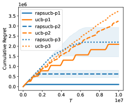
Figure 5: Regret of UCB and raps+UCB on binary tree graph with $n=20$ nodes. The last character in the label specifies the number of parent nodes.

In this section we describe an experiment aimed at showing improved regret with our approach. Other experiments that verify our theoretical findings about the number of interventions that raps takes, an analysis of the values of $\varepsilon$ and $\Delta$ in Erdős-Rényi graphs, and the results of running the combination of raps and UCB on such graphs are presented in appendix H. Here we consider the case when the underlying graph is a binary tree with $n=20$ nodes including the reward node, with the parent(s) of the reward node chosen uniformly at random. The PCM is such that the value of the root node is chosen randomly and each other node passes the value of its’ parent to its’ children with probability 0.9 and samples a value uniformly at random with probability 0.1. All nodes in the graph take on binary values. The probability of the reward node taking value $1$ is equal to the mean value of its’ parents and we set $\delta=0.01$. Even though our algorithm operates in the slow regime on trees as discussed in appendix G, we still expect to see an improvement since discovering the set of parent nodes drastically reduces the set of arms that a standard multi-armed bandit algorithm needs to choose from. The results are presented in fig. 5 with the number of parents ranging from 1 to 3. For each experiment we performed 10 independent runs and presented their means and standard deviations. The results for UCB do not change significantly and thus the error bars for this algorithm could not be seen. All our experiments (including the ones in the appendix) could be run during a day on a single laptop.

9 Conclusion

We proposed a causal bandit algorithm that does not require the knowledge of the graph structure of the causal graph including the knowledge of the essential graph. Our algorithm achieves improved regret by finding the set of parent nodes of the reward node using causal structure of the arms and thus reducing the number of arms a standard MAB algorithm needs to explore.

Appendix A Exact Number of Interventions

Algorithm 3 An algorithm equivalent to algorithm 1.

1:Set of nodes $\mathcal{V}$ of $\bm{\mathcal{G}}$ given as input

2:The parent node $P\in\mathcal{V}$ of the reward node or $\varnothing$ if there is no parent node in $\mathcal{V}$

3:Sample a random permutation $\tau$ of nodes in $\mathcal{V}$

4:$\hat{P}\leftarrow\varnothing,i\leftarrow 0$

5:for $X\in\tau$ do

6:     $i\leftarrow i+1$

7:     if $\mathcal{A}(P)\triangle\mathcal{A}(X)\cap(\tau_{1},\dots,\tau_{i-1})\neq\emptyset$ then

8:         continue     

9:     Intervene on $X$ to determine if $P\in\mathcal{D}(X)$

10:     if $P\in\mathcal{D}(X)$ then

11:         $\hat{P}\leftarrow X$      

12:return $\hat{P}$

See 6.1

Proof.

First we show that algorithm 1 is equivalent to algorithm 3 in the sense that the same sequences of nodes are intervened on by both algorithms with the same probability. Although the algorithm 3 is not practical because it uses the graph structure on 7, it allows us to present a proof for this theorem. This algorithm first samples a permutation $\tau$ of nodes in $\mathcal{V}$ and then intervenes on a node $X\in\tau$ only if none of the nodes in $\mathcal{A}(P)\triangle\mathcal{A}(X)$ appeared before $X$ in the permutation. As an example, suppose that algorithm 3 selects permutation $(X_{3},X_{2},X_{1},P)$ in fig. 1. Then the nodes intervened on by algorithm 3 are the same as the nodes intervened on by algorithm 1 in the example in section 5. This is because $X_{2}$ is a descendant of $X_{3}$ (and $X_{3}$ is not an ancestor of $P$) and therefore it will not be intervened on. Moreover, if algorithm 3 selects permutations $(X_{3},X_{1},X_{2},P)$ and $(X_{3},X_{1},P,X_{2})$, the resulting intervention sequences would be the same run of algorithm 3.

By induction on the intervened on nodes, the base case is clear since in both algorithm 1 and algorithm 3 the first node is sampled with probability $1/n$ and always intervened on. Let $\bm{\mathbf{W}}=(W_{1},\dots,W_{l})$ be a uniformly random permutation of any $l$ elements of $\mathcal{V}$ and $\bm{\mathbf{W}}^{\prime}$ be a subsequence of $\bm{\mathbf{W}}$ with an element of $W\in\bm{\mathbf{W}}$ included in $\bm{\mathbf{W}}^{\prime}$ if no element of $\mathcal{A}(P)\triangle\mathcal{A}(W)\setminus\left\{W\right\}$ was included before it. For the example in fig. 1 and sequence $\bm{\mathbf{W}}=(X_{3},X_{2})$ we have $\bm{\mathbf{W}}^{\prime}=(X_{3})$ since, as mentioned before, $X_{3}\in\mathcal{A}(P)\triangle\mathcal{A}(X_{2})\setminus\left\{X_{2}\right\}$. Note that in algorithm 1 a node could be intervened on only when it was not intervened on before and none of the non-common ancestors of that node and the parent node were intervened on. Thus, let $\mathcal{S}=\left\{X\in\mathcal{V}:\mathcal{A}(P)\triangle\mathcal{A}(X)\cup\left\{X\right\}\cap\bm{\mathbf{W}}^{\prime}=\emptyset\right\}$ be the set of nodes that could be intervened on by algorithm 1 in the next round. The probability that a node $X\in\mathcal{S}$ is sampled by algorithm 1 given the sequence $\bm{\mathbf{W}}^{\prime}$ is $1/s$, where $s=\left|\mathcal{S}\right|$. On the other hand, the probability that a node $X\in\mathcal{S}$ is intervened on next by algorithm 3 is

$$\mathbb{P}\left\{\text{$X$ is sampled before $\mathcal{A}(P)\triangle\mathcal{A}(X)\setminus\left\{X\right\}$}|\bm{\mathbf{W}}\right\}$$ (4)

$$\quad=\sum_{k=0}^{n-l-s}\mathbb{P}\left\{\bm{\mathbf{W}}_{l+1:l+k}\cap\left(\mathcal{A}(P)\triangle\mathcal{A}(X)\setminus\left\{X\right\}\right)=\emptyset\text{ and }W_{l+1+k}=X|\bm{\mathbf{W}}\right\}$$ (5)

$$\quad=\sum_{k=0}^{n-l-s}\frac{\binom{n-l-s}{k}k!(n-l-k-1)!}{(n-l)!}$$ (6)

$$\quad=\sum_{k=0}^{n-l-s}\frac{(n-l-s)!(n-l-k-1)!}{(n-l-s-k)!(n-l)!}$$ (7)

$$\quad=\frac{1}{s}\sum_{k=0}^{n-l-s}\frac{\binom{n-l-k-1}{s-1}}{\binom{n-l}{s}}=\frac{1}{s},$$ (8)

where $\bm{\mathbf{W}}_{l+1:l+k}$ consists of $k$ elements sampled uniformly at random after sampling $\bm{\mathbf{W}}$, we used the fact that there are $n-l-s$ “good“ elements from which we need to sample $k$ elements before sampling $W_{l+1+k}=X$ while the remaining elements could come in any order, and to get the last equality we used the hockey-stick identity Jones [1994]. The hockey-stick identity states that for any $n,r\in\mathbb{N}$ such that $n\geq r$ it holds that $\sum_{i=r}^{n}\binom{i}{r}=\binom{n+1}{r+1}$. By the chain rule of probability, the intermediate result holds.

Next, with $\bm{\mathbf{W}}=(W_{1},\dots,W_{n})$ being a uniformly random permutation corresponding to a run of algorithm 3, and defining $A_{X}=\left\{\text{\lx@cref{creftype~refnum}{alg:equiv} intervenes on $X$}\right\}$, $\bm{\mathbf{W}}_{<i}=(W_{1},\dots,W_{i-1})$ we can get

$$\mathbb{E}[N(\bm{\mathcal{G}},P)]=\mathbb{E}[\sum_{X\in\mathcal{V}}\mathbb{I}\left\{A_{X}\right\}]=\sum_{X\in\mathcal{V}}\mathbb{P}\left\{A_{X}\right\}$$ (9)

$$\quad=\sum_{X\in\mathcal{V}}\sum_{i=1}^{n-\left|\mathcal{A}(P)\triangle\mathcal{A}(X)\setminus\left\{X\right\}\right|}\mathbb{P}\left\{\mathcal{A}(P)\triangle\mathcal{A}(X)\setminus\left\{X\right\}\cap\bm{\mathbf{W}}_{<i}=\emptyset|W_{i}=X\right\}\mathbb{P}\left\{W_{i}=X\right\}$$ (10)

$$\quad=\sum_{X\in\mathcal{V}}\sum_{i=1}^{n-\left|\mathcal{A}(P)\triangle\mathcal{A}(X)\setminus\left\{X\right\}\right|}\frac{\binom{n-\left|\mathcal{A}(P)\triangle\mathcal{A}(X)\setminus\left\{X\right\}\right|-1}{i-1}(i-1)!(n-i)!}{(n-1)!}\cdot\frac{1}{n}$$ (11)

$$\quad=\sum_{X\in\mathcal{V}}\frac{1}{\left|\mathcal{A}(P)\triangle\mathcal{A}(X)\setminus\left\{X\right\}\right|+1}\sum_{i=1}^{n-\left|\mathcal{A}(P)\triangle\mathcal{A}(X)\setminus\left\{X\right\}\right|}\frac{\binom{n-i}{\left|\mathcal{A}(P)\triangle\mathcal{A}(X)\setminus\left\{X\right\}\right|}}{\binom{n}{\left|\mathcal{A}(P)\triangle\mathcal{A}(X)\setminus\left\{X\right\}\right|+1}}$$ (12)

$$\quad=\sum_{X\in\mathcal{V}}\frac{1}{\left|\mathcal{A}(P)\triangle\mathcal{A}(X)\setminus\left\{X\right\}\right|+1},$$ (13)

where we used the fact that to have $\mathcal{A}(P)\triangle\mathcal{A}(X)\setminus\left\{X\right\}\cap\bm{\mathbf{W}}_{<i}=\emptyset$ we need to sample $i-1$ “good“ elements from $n-\left|\mathcal{A}(P)\triangle\mathcal{A}(X)\setminus\left\{X\right\}\right|-1$ elements (since $W_{i}$ is fixed to be $X$) while the rest of the $n-i$ elements could be shuffled, and to get the last equality we used the hockey-stick identity Jones [1994]. ∎

Appendix B Logarithmic Upper Bound

See 6.3

The proof of this lemma uses the following proposition.

Proposition B.1.

For a graph $\bm{\mathcal{G}}=(\mathcal{V},\mathcal{E})$ let $\mathcal{U}\subseteq\mathcal{V}$ and $\mathcal{S}\supseteq\mathcal{D}(\mathcal{U})$, then $\mathcal{D}_{\mathcal{S}}(\mathcal{U})=\mathcal{D}(\mathcal{U})$.

Proof.

Let $X\in\mathcal{D}(\mathcal{U})$, then there is a directed path from some $U\in\mathcal{U}$ to $X$ in $\bm{\mathcal{G}}$. Each node on this path belongs to $\mathcal{D}(U)\subseteq\mathcal{D}(\mathcal{U})\subseteq\mathcal{S}$. Thus, in the graph $\bm{\mathcal{G}}_{\mathcal{S}}$ this path is preserved and we get $X\in\mathcal{D}_{\mathcal{S}}(\mathcal{U})$. Conversely, if $X\in\mathcal{D}_{\mathcal{S}}(\mathcal{U})$, then there is a directed path from some $U\in\mathcal{U}$ to $X$ in $\bm{\mathcal{G}}_{\mathcal{S}}$. Adding vertices and connections to a graph does not remove existing paths and thus there is a path from $U\in\mathcal{U}$ to $X$ in $\bm{\mathcal{G}}$ and therefore $X\in\mathcal{D}(\mathcal{U})$. ∎

Proof of lemma lemma 6.3.

In the proof we omit writing $\bm{\mathcal{C}}_{\bm{\mathcal{G}}(P)}$ and write $\bm{\mathcal{C}}$ instead for simplicity. The proof is by induction. For the base case we have $\mathcal{C}=\mathcal{V}=\mathcal{V}\setminus\mathcal{D}(\emptyset)\in\bm{\mathcal{C}}$. By induction hypothesis

$$\mathcal{C} =\mathcal{V}\setminus\mathcal{D}(\mathcal{W})\text{ for some }\mathcal{W}\subseteq\mathcal{V}\setminus\mathcal{A}(P)\text{, or}$$ (14)

$$\mathcal{C} =\bar{\mathcal{D}}(Z)\setminus\mathcal{D}_{\mathcal{D}(Z)}(\mathcal{W})\text{ for some }Z\in\mathcal{A}(P),\mathcal{W}\subseteq\mathcal{D}(Z)\setminus\mathcal{A}_{\mathcal{D}(Z)}(P).$$ (15)

Notice that in eq. 15 we have $\mathcal{D}(\mathcal{W})\subseteq\mathcal{D}(\mathcal{D}(Z)\setminus\mathcal{A}_{\mathcal{D}(Z)}(P))\subseteq\mathcal{D}(Z)$ and thus by proposition B.1 it could be rewritten as

$$C=\bar{\mathcal{D}}(Z)\setminus\mathcal{D}(\mathcal{W})\text{ for some }Z\in\mathcal{A}(P),\mathcal{W}\subseteq\mathcal{D}(Z)\setminus\mathcal{A}_{\mathcal{D}(Z)}(P).$$ (16)

Next, we will consider four cases depending on whether the condition $P\in\mathcal{D}_{\mathcal{C}}(X)$ on 9 of algorithm 1 holds and whether $\mathcal{C}$ conforms to eq. 14 or eq. 16.

1. $P\in\mathcal{D}_{\mathcal{C}}(X)$. Consider the set $\mathcal{D}(X)\setminus\mathcal{D}(\mathcal{W}^{\prime})$ for some $\mathcal{W}^{\prime}\subseteq\mathcal{D}(X)$. It consists precisely of descendants of $X$ but not $Y\in\mathcal{W}^{\prime}\subseteq\mathcal{D}(X)$. Thus, we can remove all nodes $Y\in\mathcal{D}(\mathcal{W}^{\prime})$ from the original graph $\bm{\mathcal{G}}$ and the descendants of $X$ in this new graph will be equal to $\mathcal{D}(X)\setminus\mathcal{D}(\mathcal{W}^{\prime})$:

   $$\mathcal{D}(X)\setminus\mathcal{D}(\mathcal{W}^{\prime})=\mathcal{D}_{\mathcal{V}\setminus\mathcal{D}(\mathcal{W}^{\prime})}(X).$$ (17)

   Next, we consider two subcases depending on whether $\mathcal{C}$ conforms to eq. 14 or eq. 16.

   1. $\mathcal{C}$ is such that eq. 14 holds for some $\mathcal{W}\subseteq\mathcal{V}\setminus\mathcal{A}(P)$. Then using the above, it is left to show that there exists $\mathcal{W}^{\prime}\subseteq\mathcal{D}(X)\setminus\mathcal{A}_{\mathcal{D}(X)}(P)$ such that $\mathcal{D}_{\mathcal{V}\setminus\mathcal{D}(\mathcal{W}^{\prime})}(X)=\mathcal{D}_{\mathcal{V}\setminus\mathcal{D}(\mathcal{W})}(X)=\mathcal{D}_{\mathcal{C}}(X)$ since $\bar{\mathcal{D}}(X)$ is what the recursive function will be called with in algorithm 1. For this we can set $\mathcal{W}^{\prime}=\mathcal{D}(\mathcal{W})\cap\mathcal{D}(X)$. Indeed, $\mathcal{W}$ does not contain any ancestors of $P$ and thus $\mathcal{D}(\mathcal{W})$ does not contain ancestors of $P$ in $\bm{\mathcal{G}}$ which means that $\mathcal{W}^{\prime}\cap\mathcal{A}_{\mathcal{D}(X)}(P)=\emptyset$. Moreover, $\mathcal{V}\setminus\mathcal{D}(\mathcal{W})$ removes only non-descendants of $X$ from $\bm{\mathcal{G}}$ compared to $\mathcal{V}\setminus\mathcal{D}(\mathcal{W}^{\prime})$. This is true because

      $$\mathcal{D}(X)\cap(\mathcal{V}\setminus(\mathcal{D}(\mathcal{W})\cap\mathcal{D}(X)))=\mathcal{D}(X)\setminus\mathcal{D}(\mathcal{W})\subseteq\mathcal{V}\setminus\mathcal{D}(\mathcal{W})$$ (18)

      and $\bar{\mathcal{D}}_{\mathcal{C}}(X)\in\bm{\mathcal{C}}$ follows from proposition B.1.

   2. $\mathcal{C}$ is such that eq. 16 holds for some $Z\in\mathcal{A}(P),\mathcal{W}\subseteq\mathcal{D}(Z)\setminus\mathcal{A}_{\mathcal{D}(Z)}(P)$. Similarly to the item Case I:i) for $\mathcal{W}^{\prime}=\mathcal{D}(\mathcal{W})\cap\mathcal{D}(X)$ we get

      $$\mathcal{D}(X)\cap(\mathcal{V}\setminus(\mathcal{D}(\mathcal{W})\cap\mathcal{D}(X)))=\mathcal{D}(X)\setminus\mathcal{D}(\mathcal{W})\subseteq\bar{\mathcal{D}}(Z)\setminus\mathcal{D}(\mathcal{W}),$$ (19)

      where the last step follows from the fact that $Z\in\bar{\mathcal{A}}(X)$ which is true because $X\in\mathcal{C}\subseteq\bar{\mathcal{D}}(Z)$. Additionally, $\mathcal{W}^{\prime}\subseteq\mathcal{D}(X)\setminus\mathcal{A}_{\mathcal{D}(X)}(P)$. This is true because $\mathcal{W}$ does not contain the ancestors of $P$ in $\bm{\mathcal{G}}_{\mathcal{D}(Z)}$ and $\mathcal{D}(X)$ is a subset of $\mathcal{D}(Z)$ since $Z\in\bar{\mathcal{A}}(X)$. Finally, the fact that $\bar{\mathcal{D}}_{\mathcal{C}}(X)\in\bm{\mathcal{C}}$ follows from combining the results above and proposition B.1.

2. $P\in\mathcal{D}_{\mathcal{C}}^{c}(X)$ which is equivalent to $X\in\mathcal{A}_{\mathcal{C}}^{c}(P)$. In fact, we will show that $X\not\in\mathcal{A}(P)$ by contradiction. To this end, assume that $X\in\mathcal{A}(P)$. In algorithm 1 the candidate set $\mathcal{C}$ with which the recursive function is called decreases in size during each call. At the same time, if at some point sample $Y\in\mathcal{A}(P)\cap\mathcal{A}^{c}(X)$ gets sampled, then the candidate set will consists of a subset of descendants of $Y$ to which $X$ does not belong. Thus, to sample $X$ at some point we must not have sampled such $Y$ before which means $\mathcal{A}(P)\cap\mathcal{A}^{c}(X)\subseteq\mathcal{C}$. In particular, this means that $\mathcal{A}(P)\cap\mathcal{D}(X)\subseteq\mathcal{C}$ which intern leads to $X\in\mathcal{A}_{\mathcal{C}}^{c}(P)$ which is a contradiction. Thus, $X\not\in\mathcal{A}(P)$.

   In what follows, we again consider two subscases depending on whether $\mathcal{C}$ conforms to eq. 14 or eq. 16.

   1. $\mathcal{C}=\mathcal{V}\setminus\mathcal{D}(\mathcal{W})$ for some $\mathcal{W}\subseteq\mathcal{A}^{c}(P)$. First, we show that

      $$\mathcal{D}(X)\setminus\mathcal{D}_{\mathcal{C}}(X)\subseteq\mathcal{D}(\mathcal{W}).$$ (20)

      Indeed, for $Y\in\mathcal{D}(X)\setminus\mathcal{D}_{\mathcal{C}}(X)$ there must be a directed path from $X$ to $Y$ in $\bm{\mathcal{G}}$ but not in $\bm{\mathcal{G}}_{\mathcal{V}\setminus\mathcal{D}(\mathcal{W})}$ which corresponds to the original graph with the descendants of $\mathcal{W}$ removed. Therefore, the descendants of $\mathcal{W}$ block all the directed paths from $X$ to $Y$ and therefore $Y\in\mathcal{D}(\mathcal{W})$. Next, notice that since $X\in\mathcal{A}^{c}(P)$ we can set $\mathcal{W}^{\prime}=\mathcal{W}\cup\left\{X\right\}\subseteq\mathcal{A}^{c}(P)$ and using the result above get

      $$\mathcal{C}\setminus\mathcal{D}_{\mathcal{C}}(X)=\mathcal{V}\setminus\mathcal{D}(\mathcal{W})\setminus\mathcal{D}_{\mathcal{C}}(X)=\mathcal{V}\setminus\mathcal{D}(\mathcal{W})\setminus\mathcal{D}(X)=\mathcal{V}\setminus\mathcal{D}(\mathcal{W}^{\prime})\in\bm{\mathcal{C}}.$$ (21)

   2. $\mathcal{C}=\bar{\mathcal{D}}(Z)\setminus\mathcal{D}(\mathcal{W})$ for some $Z\in\mathcal{A}(P),\mathcal{W}\subseteq\mathcal{D}(Z)\setminus\mathcal{A}_{\mathcal{D}(Z)}(P)$. Again, consider directed paths from $X$ to any $Y\in\mathcal{D}(X)\setminus\mathcal{D}_{\mathcal{C}}(X)$. Note that $\mathcal{D}(X)\setminus\mathcal{D}_{\mathcal{C}}(X)=\mathcal{D}_{\bar{\mathcal{D}}(Z)}(X)\setminus\mathcal{D}_{\bar{\mathcal{D}}(Z)\setminus\mathcal{D}(\mathcal{W})}(X)$ where we used proposition B.1 with the fact that $X\in\bar{\mathcal{D}}(Z)$ which implies $\mathcal{D}(X)\subseteq\bar{\mathcal{D}}(Z)$, and the definition of $\mathcal{C}$. Similarly to the previous item we get that removing the set $\mathcal{D}(\mathcal{W})$ from $\bm{\mathcal{G}}_{\bar{\mathcal{D}}(Z)}$ removes all paths from $X$ to $Y$ in this graph and thus $Y\in\mathcal{D}(\mathcal{W})$ or $\mathcal{D}(X)\setminus\mathcal{D}_{\mathcal{C}}(X)\subseteq\mathcal{D}(\mathcal{W})$. Setting $\mathcal{W}^{\prime}=\mathcal{W}\cup\left\{X\right\}$ as before gives $\mathcal{W}^{\prime}\subseteq\mathcal{D}(Z)\setminus\mathcal{A}_{\mathcal{D}(Z)}(P)$ since $X\in\bar{\mathcal{D}}(Z)$ and as stated above $X\not\in\mathcal{A}(P)$. Thus, by proposition B.1 we get the desired result.∎

See 6.4

Proof.

Based on the definition of algorithm 1, it is straightforward to see that the following recursion holds

$$T(\mathcal{C})=\frac{1}{\left|\mathcal{C}\right|}\sum_{X\in\mathcal{A}_{\mathcal{C}}(P)}T(\bar{\mathcal{D}}_{\mathcal{C}}(X))+\frac{1}{\left|\mathcal{C}\right|}\sum_{X\in\mathcal{A}_{\mathcal{C}}^{c}(P)}T(\mathcal{D}_{\mathcal{C}}^{c}(X))+1,$$ (22)

where $T(\mathcal{C})$ denotes the number of interventions performed by the recursive function in algorithm 1 given candidate set $\mathcal{C}$. We will show that $T(\mathcal{C})\leq c^{\prime}\log\left|\mathcal{C}\right|+c\log^{k}(n)$ for some $c^{\prime}>0$ by considering two cases: $\left|\mathcal{C}\right|\leq c\log(n)$ and $\left|\mathcal{C}\right|>c\log(n)$. The case where $\left|\mathcal{C}\right|\leq c\log(n)$ is straightforward since each node in $\mathcal{C}$ is intervened on at most once and $\left|\mathcal{C}\right|\leq c\log^{k}(n)$.

Next, consider the case $\left|\mathcal{C}\right|>c\log^{k}(n)$. We provide a proof for the case when $\left|\mathcal{H}_{\mathcal{C}}(\alpha)\right|\geq\beta\left|\mathcal{C}\right|$ then comment on why the result holds when $\left|\mathcal{A}_{\mathcal{C}}(P)\right|\geq\gamma\left|\mathcal{C}\right|$. By lemma 6.3 we have that for all $X\in\mathcal{A}_{\mathcal{C}}(P)$ it holds that $\bar{\mathcal{D}}_{\mathcal{C}}(X)\in\bm{\mathcal{C}}$ and for all $X\in\mathcal{A}_{\mathcal{C}}^{c}(P)$ it holds that $\mathcal{D}_{\mathcal{C}}^{c}(X)\in\bm{\mathcal{C}}$, thus the condition of the theorem holds for the recursive calls and we can use induction hypothesis after which it is left to check that

$$\frac{c^{\prime}}{\left|\mathcal{C}\right|} \sum_{X:X\in\mathcal{A}_{\mathcal{C}}(P)\wedge\left|\mathcal{D}_{\mathcal{C}}(X)\right|>1}\log(\left|\mathcal{D}_{\mathcal{C}}(X)\right|-1)+\frac{c^{\prime}}{\left|\mathcal{C}\right|}\sum_{X\in\mathcal{A}_{\mathcal{C}}^{c}(P)}\log(\left|\mathcal{C}\right|-\left|\mathcal{D}_{\mathcal{C}}(X)\right|)+1$$ (23)

$$\quad+\frac{c}{\left|\mathcal{C}\right|}\sum_{X\in\mathcal{A}_{\mathcal{C}}(P)}\log^{k}(n)+\frac{c}{\left|\mathcal{C}\right|}\sum_{X\in\mathcal{A}_{\mathcal{C}}^{c}(P)}\log^{k}(n)$$ (24)

is bounded above by $c^{\prime}\log\left|\mathcal{C}\right|+c\log^{k}(n)$. First, note that the eq. 24 is bounded by $c\log^{k}(n)$ since $\mathcal{A}_{\mathcal{C}}(X)\cup\mathcal{A}_{\mathcal{C}}^{c}(X)=\mathcal{C}$. Next, consider the eq. 23. Note that for $X\not\in\mathcal{H}_{\mathcal{C}}(\alpha)$ we can upper bound $\left|\mathcal{D}_{\mathcal{C}}(X)\right|-1$ and $\left|\mathcal{C}\right|-\left|\mathcal{D}_{\mathcal{C}}(X)\right|$ by $\left|\mathcal{C}\right|$. At the same time, for $X\in\mathcal{H}_{\mathcal{C}}(\alpha)$ we have $\left|\mathcal{C}\right|-\left|\mathcal{D}_{\mathcal{C}}(X)\right|\leq(1-\alpha)\left|\mathcal{C}\right|$. Then our goal is to show

$$\frac{c^{\prime}(\left|\mathcal{C}\right|-\left|\mathcal{H}_{\mathcal{C}}(\alpha)\right|)}{\left|\mathcal{C}\right|}\log\left|\mathcal{C}\right|+\frac{c^{\prime}\left|\mathcal{H}_{\mathcal{C}}(\alpha)\right|}{\left|\mathcal{C}\right|}\log((1-\alpha)\left|\mathcal{C}\right|)+1$$ (25)

$$\qquad\leq c^{\prime}\log\left|\mathcal{C}\right|=\frac{c^{\prime}(\left|\mathcal{C}\right|-\left|\mathcal{H}_{\mathcal{C}}(\alpha)\right|)}{\left|\mathcal{C}\right|}\log\left|\mathcal{C}\right|+\frac{c^{\prime}\left|\mathcal{H}_{\mathcal{C}}(\alpha)\right|}{\left|\mathcal{C}\right|}\log\left|\mathcal{C}\right|,$$ (26)

rearranging we get

$$\frac{\left|\mathcal{C}\right|}{c^{\prime}\left|\mathcal{H}_{\mathcal{C}}(\alpha)\right|}\leq\log\frac{1}{1-\alpha}=\log\left(\frac{\alpha}{1-\alpha}+1\right).$$ (27)

Notice that since for any $x>-1$ it holds that $\frac{x}{1+x}\leq\log(x+1)$, it suffices to show

$$\frac{\left|\mathcal{C}\right|}{c^{\prime}\left|\mathcal{H}_{\mathcal{C}}(\alpha)\right|}\leq\alpha\iff\left|\mathcal{C}\right|\leq c^{\prime}\left|\mathcal{H}_{\mathcal{C}}(\alpha)\right|\alpha.$$ (28)

From our assumption on $\left|\mathcal{H}_{\mathcal{C}}(\alpha)\right|$ it suffices to pick $c^{\prime}\geq\frac{1}{\alpha\beta}$. For the base case consider $\mathcal{C}=\left\{X,Y\right\}$ then for $X\neq P$ we have that either there is a single edge $P\rightarrow X$ or $P$ is disconnected with $X$ for the condition of the theorem to hold. Then the recursion in eq. 22 could be rewritten as

$$T(\left\{X,Y\right\})=\frac{1}{2}T(\left\{Y\right\})+\frac{1}{2}T(\left\{X\right\})+1,$$ (29)

from which it follows that

$$T(\left\{X,Y\right\})=2\leq c\log(2).$$ (30)

For the case when $\left|\mathcal{A}_{\mathcal{C}}(P)\right|\geq\gamma\left|\mathcal{C}\right|$ consider the set $\mathcal{H}^{\prime}$ of size at least $\frac{\gamma}{2}\left|\mathcal{C}\right|$ of the ancestors of $P$ which are closest to $P$ in the topologically sorted order in the graph $\bm{\mathcal{G}}_{\mathcal{C}}$. Each node $X\in\mathcal{H}^{\prime}$ has at most $\left|\mathcal{C}\right|-\frac{\gamma}{2}\left|\mathcal{C}\right|$ descendants. The rest of the proof follows similar steps as for the case when $\left|\mathcal{H}_{\mathcal{C}}(\alpha)\right|\geq\beta\left|\mathcal{C}\right|$. ∎

Appendix C Fast Parent Discovery in Erdős-Rényi Graphs

In this subsection we show that Erdős-Rényi graphs satisfy the condition for fast discovery of the parent node for sufficiently large values of $p$. We first state the following theorem.

Theorem C.1.

Let $\bm{\mathcal{G}}_{n,p}$ be Erdős-Rényi random DAG with probability of each edge between $n$ nodes being equal to $p$. Assume $p\geq 1-\left(\frac{1-c}{n-1}\right)^{1/(n-1)}$ for some constant $c\in[0,1]$, and denote by $X,Y$ the first and last nodes in the topological order, respectively. It holds that

$$\mathbb{E}\left|\mathcal{D}(X)\right| \geq cn,\text{ and}$$ (31)

$$\mathbb{E}\left|\mathcal{A}(Y)\right| \geq cn.$$ (32)

Proof.

In the proof we show by induction that the expected number of descendants of the root node (the first node in topological order) is lower bounded by $cn$. The expected number of the ancestors could be lower bounded using the same reasoning. Denote by $p_{n,i}$ the probability that there are exactly $i$ descendants of the root node in the graph $\bm{\mathcal{G}}_{n,p}$ and note that

$$\mathbb{E}\left|\mathcal{D}(X)\right|=\sum_{i=1}^{n}ip_{n,i}.$$ (33)

Furthermore, $p_{n,i}$ satisfies the following recursion:

$$p_{n,i} =(1-(1-p)^{i-1})p_{n-1,i-1}+(1-p)^{i}p_{n-1,i}$$ (34)

$$=p_{n-1,i-1}+(1-p)^{i-1}((1-p)p_{n-1,i}-p_{n-1,i-1}),$$ (35)

with $p_{1,1}=1$ and $p_{n,i}=0$ if $i>n$ or $i=0$. Thus, we can write

$$\mathbb{E}\left|\mathcal{D}(X)\right| =\sum_{i=1}^{n}ip_{n-1,i-1}+\sum_{i=1}^{n}i(1-p)^{i-1}((1-p)p_{n-1,i}-p_{n-1,i-1})$$ (36)

$$=\sum_{i=1}^{n}ip_{n-1,i-1}-\sum_{i=1}^{n}(1-p)^{i-1}p_{n-1,i-1}$$ (37)

$$\quad+\sum_{i=1}^{n}\left[i(1-p)^{i}p_{n-1,i}-(i-1)(1-p)^{i-1}p_{n-1,i-1}\right].$$ (38)

Note that

$$\sum_{i=1}^{n}\left[i(1-p)^{i}p_{n-1,i}-(i-1)(1-p)^{i-1}p_{n-1,i-1}\right]=0$$ (39)

as a telescoping sum and by induction hypothesis we have that

$$\sum_{i=1}^{n}ip_{n-1,i-1}=\sum_{i=1}^{n}(i-1)p_{n-1,i-1}+\sum_{i=1}^{n}p_{n-1,i-1}\geq c(n-1)+1,$$ (40)

therefore it is left to prove

$$\sum_{i=1}^{n}(1-p)^{i-1}p_{n-1,i-1}\leq 1-c.$$ (41)

To prove this we first show that $p_{n,i}\leq(1-p)^{n-i}$, again by induction. This holds for $n=1$ and all $i$ or $i=0$ and all $n>1$. Furthermore by induction hypothesis we have

$$p_{n,i} \leq(1-(1-p)^{i-1})(1-p)^{n-i}+(1-p)^{i}(1-p)^{n-1-i}$$ (42)

$$=(1-p)^{n-i}+(1-p)^{n-1}+(1-p)^{n-1}=(1-p)^{n-i}.$$ (43)

Using this result together with the fact that $p_{n-1,0}=0$ we have

$$\sum_{i=1}^{n}(1-p)^{i-1}p_{n-1,i-1}\leq(n-1)(1-p)^{n-1}\leq 1-c,$$ (44)

where the last inequality follows from the assumption of the theorem. To finish the proof, note that for $n=1$ we have $\mathbb{E}\left|\mathcal{D}(X)\right|=1\geq c$. ∎

See 6.5

Proof.

From our lower bound on $p$ and theorem C.1 it follows that for all subgraphs of size at least $\log^{k}n$ the first and last nodes in the topological order have at least $cn$ descendants and ancestors respectively. Let $\mathcal{C}$ be an arbitrary candidate set of size larger than $4\log^{k}n$ considered by algorithm 1 when run on the graph $\bm{\mathcal{G}}_{n,p}$. Let $j\in[m]$ with $m=\left|\mathcal{C}\right|$ be the index of $P$ in the topologically sorted order in the subgraph of $\bm{\mathcal{G}}_{m,p}$ over nodes in $\mathcal{C}$. We will comment bellow on the situation when $P\not\in\mathcal{C}$. We consider two cases. First, if $j\leq m/2$, then consider $m/4$ subgraphs each consisting of $m-m/2-i$ last nodes for $i\in[{m/4}]$ of the original graph $\bm{\mathcal{G}}_{n}$. The size of each of these subgraph is at least $\log^{k}n$ and by theorem C.1 we have that each node at index ${m/2}+i-1$ in the topological order of the original graph $\bm{\mathcal{G}}_{m}$ has at least $c{m/4}$ descendants. Since there are ${m/4}$ such nodes, the first condition of theorem 6.4 is satisfied. The same happens for the cases when $P\not\in\mathcal{C}$ because in that case all the nodes in $\mathcal{C}$ are non-ancestors of $P$ since for $P\not\in\mathcal{C}$ it must be the case that the algorithm intervened on $P$ at some point before considering $\mathcal{C}$. Second, if $j>{m/2}$, then by theorem C.1 we have that the number of ancestors of $P$ is at least $c{n/2}$ which means that the second condition of theorem 6.4 is satisfied. ∎

Remark C.2.

Note that since $(1-1/n)^{n}\leq e^{-1}$ we have $\log(n/c)\log\left(1-1/n\right)\leq-\frac{\log(n/c)}{n}$ and thus $\left(1-1/n\right)^{\log(n/c)}\leq\left(\frac{c}{n}\right)^{1/n}$. Using this together with the Bernoulli inequality $(1+x)^{r}\geq 1+rx$ for $x\geq-1$ and $r\geq 1$ we get that assuming $\log^{k}n\geq 1+\max(1,(1-c)e)$ the condition of corollary 6.5 is satisfied for $p\geq\frac{\log\left(\log^{k}(n)-1\right)-\log(1-c)}{\log^{k}(n)-1}$. Additionally, by using L’Hópital’s rule and the fact that $\lim_{n\to\infty}\left(1/n\right)^{1/n}=1$, we get that the two lower bounds for $p$ presented in corollary 6.5 and here are asymptotically equivalent.

Appendix D Sublinear Upper Bound

See 6.6

Proof.

Let $A_{X}=\left\{\text{the algorithm intervenes on the node $X$}\right\}$, then

$$\mathbb{E}[N(\bm{\mathcal{G}},P)]=\mathbb{E}[\sum_{X\in\mathcal{V}}\mathbb{I}\left\{A_{X}\right\}]=\sum_{X\in\mathcal{V}}\mathbb{P}(A_{X}).$$ (45)

We split the sum above into three parts. First, consider the nodes $X$ that are at distance at most $m$ from the parent node for some $m$ to be specified later. There are at most $d^{m+1}$ such nodes and for each of them we bound the probability $\mathbb{P}(A_{X})$ by 1. Similarly, for all nodes $X$ such that there is no collider-free path between $P$ and $X$ we also bound the probability $\mathbb{P}(A_{X})$ by 1. Each of the leftover nodes has a collider-free path of length at least $m$ to $P$. We will show that this means that the probability $\mathbb{P}(A_{X})\leq 2/m$. Define

$$B_{X}=\left\{\text{the algorithm intervenes on the node $P$ before intervening on the node $X$}\right\},$$ (46)

then using the law of total probability we can write

$$\mathbb{P}(A_{X})=\mathbb{P}(A_{X}|B_{X})\mathbb{P}(B_{X})+\mathbb{P}(A_{X}|B_{X}^{c})\mathbb{P}(B_{X}^{c}),$$ (47)

where $B_{X}^{c}$ stands for the complement of the event $B_{X}$, i.e.

$$B_{X}^{c}=\left\{\text{the algorithm intervenes on node $P$ after intervening on the node $X$}\right\}.$$ (48)

Consider the probability $\mathbb{P}(A_{X}|B_{X})$. For this probability not to be zero it must be the case that the node $X$ is a descendant of the parent node $P$. Therefore, there must be a directed path of length at least $m$ from $P$ to $X$. Note that any node on this path except for the node $P$ cannot be intervened on before the node $X$ is intervened on. Therefore, by the time the algorithm intervenes on the node $X$ there are at least $m$ nodes in the set of candidate nodes from which it has to sample the node $X$ and hence

$$\mathbb{P}(A_{X}|B_{X})\leq\frac{1}{m}.$$ (49)

Next, consider the probability $\mathbb{P}(B_{X}^{c})$. If there is a directed path from $P$ to $X$, then no node on this path could have been intervened on before the round at which the algorithm intervenes on $X$ since otherwise $X$ would have been removed from the candidate set. Similarly, if there is a directed path from $X$ to $P$, then intervening on any node on the path means excluding $X$ from the candidate set. Thus, in these two cases $\mathbb{P}(B_{X}^{c})\leq 1/(m+1)$ as there are at least $m+1$ nodes on the path of length at least $m$. Lastly, consider the case when there are no directed paths between $P$ and $X$. Since for this $X$ there exists a collider-free path, there must be a path containing exactly one ancestor of both $X$ and $P$. Intervening on any node on this path other than the node which is an ancestor of both $X$ and $P$ means excluding $X$ from the candidate set because the intervened on node would be an ancestor of $X$ or $P$ but not both. Thus, there are at least $m$ nodes in the candidate set by the time the algorithm intervenes on $X$ and therefore

$$\mathbb{P}(B_{X}^{c})\leq\frac{1}{m}.$$ (50)

Bounding the other probabilities by one gives $\mathbb{P}(A_{X})\leq 2/m$. Bounding the number of nodes in the third group by $n$ and combining all of the above we get

$$\mathbb{E}[N(\bm{\mathcal{G}},P)]=\mathcal{O}\left(d^{m+1}+\frac{n}{m}+\frac{n}{\log_{d}(n)}\right).$$ (51)

Finally, setting $m=\log_{d}\left(\frac{n}{\log_{d}(n)}\right)-1$ finishes the proof. ∎

Appendix E Regret Bounds

E.1 Cumulative Regret

Lemma E.1.

Let

$$A_{X,\bm{\mathbf{Z}}} =\left\{\exists x\in[K],\bm{\mathbf{z}}\in[K]^{\left|\bm{\mathbf{Z}}\right|}:\left|\bar{R}-\bar{R}^{do(X=x,\bm{\mathbf{Z}}=\bm{\mathbf{z}})}\right|>\Delta/2\right\},$$

$$D_{X,Y,\bm{\mathbf{Z}}} =\Bigl{\{}\exists x,y\in[K],\bm{\mathbf{z}}\in[K]^{\left|\bm{\mathbf{Z}}\right|}:\left|\hat{P}(Y=y)-\hat{P}(Y=y|do(X=x,\bm{\mathbf{Z}}=\bm{\mathbf{z}}))\right|>\varepsilon/2\Bigr{\}}$$

for any $X,Y\in\mathcal{V}$, $\bm{\mathbf{Z}}\subseteq\mathcal{P}$ with nodes being the last in some topological order of $\mathcal{P}$ and $A_{X,\bm{\mathbf{Z}}}^{c},D_{X,Y,\bm{\mathbf{Z}}}^{c}$ be their compliments. Define $E$ as the event that for every node we correctly determine its descendants and whether it is an ancestor of $P$ using the criteria described in section 5.1, i.e.

$$E=\bigcap_{\bm{\mathbf{Z}}}\bigcap_{X\in\mathcal{A}(P)}A_{X,\bm{\mathbf{Z}}}\cap\bigcap_{X\in\mathcal{A}^{c}(P)}A_{X,\bm{\mathbf{Z}}}^{c}\cap\bigcap_{X\in\mathcal{V}}\Bigl{(}\bigcap_{Y\in\bar{\mathcal{D}}(X)}D_{X,Y,\bm{\mathbf{Z}}}\cap\bigcap_{Y\in\mathcal{D}^{c}(X)}D_{X,Y,\bm{\mathbf{Z}}}^{c}\Bigr{)},$$

where the intersection with respect to $\bm{\mathbf{Z}}$ is over all possible sequences of last elements of $\mathcal{P}$ in all topological orders. Then it holds that $\mathbb{P}\left\{E\right\}\geq 1-\delta$ if $B=\max\left\{\frac{32}{\Delta^{2}}\log\left(\frac{8nK(K+1)^{n}}{\delta}\right),\frac{8}{\varepsilon^{2}}\log\left(\frac{8n^{2}K^{2}(K+1)^{n}}{\delta}\right)\right\}$.

Proof.

By Hoeffding’s inequality for bounded random variables for fixed $X,Y\in\mathcal{V}$ with $X\in\mathcal{A}(Y)$, $\bm{\mathbf{Z}}\subseteq\mathcal{P}$, $x,y\in[K]$ and $\bm{\mathbf{z}}\in[K]^{\left|\bm{\mathbf{Z}}\right|}$ it holds that

$$\left|\hat{P}(Y=y|do(X=x,\bm{\mathbf{Z}}=\bm{\mathbf{z}}))-\mathbb{P}\left\{Y=y|do(X=x,\bm{\mathbf{Z}}=\bm{\mathbf{z}})\right\}\right|\geq$$ (52)

$$\quad\geq\sqrt{\frac{1}{2B}\log\left(\frac{8n^{2}K^{2}(K+1)^{n}}{\delta}\right)}$$ (53)

with probability at most $\frac{\delta}{4n^{2}K^{2}(K+1)^{n}}$ and

$$\left|\hat{P}(Y=y|do(\bm{\mathbf{Z}}=\bm{\mathbf{z}}))-\mathbb{P}\left\{Y=y|do(\bm{\mathbf{Z}}=\bm{\mathbf{z}})\right\}\right|\geq\sqrt{\frac{1}{2B}\log\left(\frac{8}{\delta}\right)}$$ (54)

with probability at most $\frac{\delta}{4nK(K+1)^{n}}$. Additionally, by Hoeffding’s inequality for $1$-subgaussian random variables we have that for fixed $X\in\mathcal{V}$ and $x\in[K]$ it holds that

$$\left|\mathbb{E}[R|do(X=x,\bm{\mathbf{Z}}=\bm{\mathbf{z}})]-\bar{R}^{do(X=x,\bm{\mathbf{Z}}=\bm{\mathbf{z}})}\right|\geq\sqrt{\frac{2}{B}\log\left(\frac{8nK(K+1)^{n}}{\delta}\right)}$$ (55)

with probability at most $\frac{\delta}{4nK(K+1)^{n}}$. Moreover,

$$\left|\bar{R}^{do(\bm{\mathbf{Z}}=\bm{\mathbf{z}})}-\mathbb{E}[R|do(\bm{\mathbf{Z}}=\bm{\mathbf{z}})]\right|\geq\sqrt{\frac{2}{B}\log\left(\frac{8(K+1)^{n}}{\delta}\right)}$$ (56)

with probability at most $\frac{\delta}{4(K+1)^{n}}$. Consider the event which is the union of the above bad events. Since for $\bm{\mathbf{Z}}$ there are $\sum_{\ell=0}^{\left|\mathcal{P}\right|}\binom{\left|\mathcal{P}\right|}{\ell}K^{\ell}=(K+1)^{\left|\mathcal{P}\right|}$ choices, by union bound we have that the probability of this bad event is at most $\delta$. Note that under the complement of this bad event for $X\not\in\mathcal{A}(P)$ and all $x\in[K],\bm{\mathbf{z}}\in[K]^{\left|\bm{\mathbf{Z}}\right|}$ by 4.2 and the choice of $B$ as in the statement of lemma E.1 we have

$$\left|\bar{R}^{do(\bm{\mathbf{Z}}=\bm{\mathbf{z}})}-\bar{R}^{do(X=x,\bm{\mathbf{Z}}=\bm{\mathbf{z}})}\right| \leq\left|\bar{R}^{do(\bm{\mathbf{Z}}=\bm{\mathbf{z}})}-\mathbb{E}[R|do(\bm{\mathbf{Z}}=\bm{\mathbf{z}})]\right|$$ (57)

$$\quad+\left|\bar{R}^{do(X=x,\bm{\mathbf{Z}}=\bm{\mathbf{z}})}-\mathbb{E}[R|do(X=x,\bm{\mathbf{Z}}=\bm{\mathbf{z}})]\right|$$ (58)

$$\leq\Delta/2,$$ (59)

and for some $x\in[K],\bm{\mathbf{z}}\in[K]^{\left|\bm{\mathbf{Z}}\right|}$

$$\left|\bar{R}^{do(\bm{\mathbf{Z}}=\bm{\mathbf{z}})}-\bar{R}^{do(X=x,\bm{\mathbf{Z}}=\bm{\mathbf{z}})}\right| \geq\left|\mathbb{E}[R|do(\bm{\mathbf{Z}}=\bm{\mathbf{z}})]-\mathbb{E}[R|do(X=x,\bm{\mathbf{Z}}=\bm{\mathbf{z}})]\right|$$ (60)

$$\quad-\left|\bar{R}^{do(\bm{\mathbf{Z}}=\bm{\mathbf{z}})}-\mathbb{E}[R|do(\bm{\mathbf{Z}}=\bm{\mathbf{z}})]\right|$$ (61)

$$\quad-\left|\mathbb{E}[R|do(X=x,\bm{\mathbf{Z}}=\bm{\mathbf{z}})-\bar{R}^{do(X=x,\bm{\mathbf{Z}}=\bm{\mathbf{z}})}]\right|$$ (62)

$$>\Delta/2,$$ (63)

Similarly, under the complement of the same event we get that for $Y\not\in\mathcal{D}(X)$ and all $x,y\in[K],\bm{\mathbf{z}}\in[K]^{\left|\bm{\mathbf{Z}}\right|}$ it holds that

$$\left|\hat{P}(Y=y|do(\bm{\mathbf{Z}}=\bm{\mathbf{z}}))-\hat{P}(Y=y|do(X=x,\bm{\mathbf{Z}}=\bm{\mathbf{z}})\right|\leq$$ (64)

$$\quad\leq\left|\hat{P}(Y=y|do(\bm{\mathbf{Z}}=\bm{\mathbf{z}}))-\mathbb{P}\left\{Y=y|do(\bm{\mathbf{Z}}=\bm{\mathbf{z}})\right\}\right|$$ (65)

$$\quad\quad+\left|\hat{P}(Y=y|do(X=x,\bm{\mathbf{Z}}=\bm{\mathbf{z}}))-\mathbb{P}\left\{Y=y|do(X=x,\bm{\mathbf{Z}}=\bm{\mathbf{z}})\right\}\right|$$ (66)

$$\quad\leq\varepsilon/2,$$ (67)

and if $Y\in\mathcal{D}(X)$, then for some $x,y\in[K],\bm{\mathbf{z}}\in[K]^{\left|\bm{\mathbf{Z}}\right|}$

$$\left|\hat{P}(Y=y|do(\bm{\mathbf{Z}}=\bm{\mathbf{z}}))-\hat{P}(Y=y|do(X=x,\bm{\mathbf{Z}}=\bm{\mathbf{z}})\right|\geq$$ (68)

$$\quad\geq\left|\mathbb{P}\left\{Y=y|do(X=x,\bm{\mathbf{Z}}=\bm{\mathbf{z}})\right\}-\mathbb{P}\left\{Y=y|do(\bm{\mathbf{Z}}=\bm{\mathbf{z}})\right\}\right|$$ (69)

$$\quad\quad-\left|\mathbb{P}\left\{Y=y|do(X=x,\bm{\mathbf{Z}}=\bm{\mathbf{z}})\right\}-\hat{P}(Y=y|do(X=x,\bm{\mathbf{Z}}=\bm{\mathbf{z}}))\right|$$ (70)

$$\quad\quad-\left|\hat{P}(Y=y|do(\bm{\mathbf{Z}}=\bm{\mathbf{z}}))-\mathbb{P}\left\{Y=y|do(\bm{\mathbf{Z}}=\bm{\mathbf{z}})\right\}\right|>\varepsilon/2.$$ (71)

∎

See 4.3

Proof.

By lemma lemma E.1 it holds that for every node we can correctly identify whether that node is an ancestor of $P$ and all the descendants of that node with probability at least $1-\delta$ using the criteria described in section 5.1. That means that algorithm 1 will correctly discover the parent node under the same good event in $B\mathbb{E}[N(\bm{\mathcal{G}},P)]\sum_{\ell=1}^{\left|\mathcal{P}\right|+1}K^{\ell}\preceq B\mathbb{E}[N(\bm{\mathcal{G}},P)]K^{\left|\mathcal{P}\right|+1}$ interventions since to discover each new parent we need to perform interventions over all possible values of the previously discovered parents and all the remaining candidate nodes. Subsequently running a standard bandit algorithm such as UCB to find an optimal intervention on $P$ leads to regret bound of $\sum_{\bm{\mathbf{x}}\in[K]^{\left|\mathcal{P}\right|}}\Delta_{\mathcal{P}=\bm{\mathbf{x}}}\left(1+\frac{\log{T}}{\Delta_{\mathcal{P}=\bm{\mathbf{x}}}^{2}}\right)$ Lattimore and Szepesvári [2020]. ∎

E.2 Simple Regret

In this subsection we provide an upper bound on simple regret. First, similar to how it is done in the main text, we define conditional simple regret:

$$r_{\mathcal{L}}^{T}(\bm{\mathcal{G}},\mathcal{P}|E)=\max_{\bm{\mathbf{X}}\subseteq\mathcal{V}}\max_{\bm{\mathbf{x}}\in[K]^{\left|\bm{\mathbf{X}}\right|}}\mathbb{E}[R|do(\bm{\mathbf{X}}=\bm{\mathbf{x}})]-\mathbb{E}[R|do(\bm{\mathbf{X}}_{T+1}=\bm{\mathbf{x}}_{T+1}),E],$$ (72)

where $E$ is the event that all descendants of any node in $\mathcal{V}$ are correctly identified together with whether any node is an ancestor of $\mathcal{P}$, defined in lemma E.1. Suppose that the learner runs a standard bandit algorithm that is designed to minimize cumulative regret, for example, UCB, from round $N(\bm{\mathcal{G}},\mathcal{P})+1$ to round $T$. After that the final intervention $do(X=x)$ for arbitrary $x\in[K]$ and $X\in\mathcal{V}$ is sampled with probability

$$\frac{1}{T}\sum_{t=1}^{T}\mathbb{I}\left\{I_{t}=do(X=x)\right\},$$ (73)

where $I_{t}$ is the intervention performed in round $t$. Standard conversion of cumulative regret bound to simple regret bound [see e.g., Lattimore and Szepesvári, 2020, Proposition 33.2] leads to corollary E.2 stated below.

Corollary E.2.

For the learner described above we can bound conditional simple regret as follows:

$$r_{\mathcal{L}}^{T}(\bm{\mathcal{G}},\mathcal{P}|E) \preceq\frac{1}{T}\max\left\{\frac{1}{\Delta^{2}},\frac{1}{\varepsilon^{2}}\right\}K^{\left|\mathcal{P}\right|+2}\mathbb{E}[N(\bm{\mathcal{G}},\mathcal{P})]\log\left(\frac{nK^{n}}{\delta}\right)$$ (74)

$$\quad+\frac{1}{T}\sum_{\bm{\mathbf{x}}\in[K]^{\left|\mathcal{P}\right|}}\Delta_{\mathcal{P}=\bm{\mathbf{x}}}\left(1+\frac{\log{T}}{\Delta_{\mathcal{P}=\bm{\mathbf{x}}}^{2}}\right).$$ (75)

Appendix F Generalization to Multiple Parent Nodes

Algorithm 4 Full version of raps for unknown number of parents

1:Set of nodes $\mathcal{V}$ of $\bm{\mathcal{G}}$, $\varepsilon,\Delta$, probability of incorrect parent set estimate $\delta$

2:Estimated set of parent nodes $\hat{\mathcal{P}}$

3:$\hat{\mathcal{P}}\leftarrow\emptyset,\mathcal{S}\leftarrow\emptyset,\hat{P}\leftarrow\varnothing,\mathcal{C}\leftarrow\mathcal{V},\mathcal{D}^{\prime}\leftarrow\emptyset$ $\triangleright$ $\mathcal{D}^{\prime}$ is the set of descendants of last ancestor of $R$

4:$B\leftarrow\max\left\{\frac{32}{\Delta^{2}}\log\left(\frac{8nK(K+1)^{n}}{\delta}\right),\frac{8}{\varepsilon^{2}}\log\left(\frac{8n^{2}K^{2}(K+1)^{n}}{\delta}\right)\right\}$

5:Observe $B$ samples from PCM and compute $\bar{R}$ and $\hat{P}(X)$ for all $X\in\mathcal{V}$

6:while $\mathcal{C}\neq\emptyset$ do

7:     $X\sim\mathcal{U}nif(\mathcal{C})$

8:     for $x\in[K]$ and $\bm{\mathbf{z}}\in[K]^{\left|\hat{\mathcal{P}}\right|}$ do

9:         Perform $B$ interventions $do(X=x,\hat{\mathcal{P}}=\bm{\mathbf{z}})$

10:         Compute $\bar{R}^{do(X=x,\hat{\mathcal{P}}=\bm{\mathbf{z}})},\hat{P}(Y|do(X=x,\hat{\mathcal{P}}=\bm{\mathbf{z}}))$ for all $Y\in\mathcal{V}$      

11:     Estimate descendants of $X$:

$$\mathcal{D}\leftarrow\biggl{\{}Y\in\mathcal{V} \mid\exists x\in[K],\bm{\mathbf{z}}\in[K]^{\left|\hat{\mathcal{P}}\right|},$$

$$\text{ such that }\left|\hat{P}(Y|do(\hat{\mathcal{P}}=\bm{\mathbf{z}}))-\hat{P}(Y|do(X=x,\hat{\mathcal{P}}=\bm{\mathbf{z}}))\right|>\varepsilon/2\biggr{\}}$$

12:     if $\exists x\in[K],\bm{\mathbf{z}}\in[K]^{\left|\hat{\mathcal{P}}\right|}$ such that $\left|\bar{R}^{do(\hat{\mathcal{P}}=\bm{\mathbf{z}})}-\bar{R}^{do(X=x,\hat{\mathcal{P}}=\bm{\mathbf{z}})}\right|>\Delta/2$ then

13:         $\mathcal{C}\leftarrow\mathcal{D}\setminus\left\{X\right\}$

14:         $\hat{P}\leftarrow X,\mathcal{D}^{\prime}\leftarrow\mathcal{D}$

15:     else

16:         $\mathcal{C}\leftarrow\mathcal{C}\setminus\mathcal{D}$

17:         $\mathcal{S}\leftarrow\mathcal{S}\cup\mathcal{D}$      

18:     if $\mathcal{C}=\emptyset$ and $\hat{P}\neq\varnothing$ then

19:         $\hat{\mathcal{P}}\leftarrow\hat{\mathcal{P}}\cup\left\{\hat{P}\right\}$

20:         $\mathcal{S}\leftarrow\mathcal{S}\cup\mathcal{D}^{\prime}$

21:         $\mathcal{C}\leftarrow\mathcal{V}\setminus\mathcal{S}$

22:         $\hat{P}\leftarrow\varnothing$      

23:return $\hat{\mathcal{P}}$

See 7.1

Proof.

As noted in the main text, algorithm 2 discovers the parent nodes in a reverse topological order, let $\tau\in\bm{\tau}(\mathcal{P})$ be such an order and $i=\left|\hat{\mathcal{P}}\right|\leq\left|\mathcal{P}\right|$ be a number of the iteration of the while loop in algorithm 2. First, assume $i<\left|\mathcal{P}\right|$. We argue that the expected number of interventions during a call of algorithm 1 is the same as the expected number of interventions done by algorithm 1 when there is only one parent node $P$ which is equal to the $(\left|\mathcal{P}\right|-i)$-th element of $\tau$ and $\hat{\mathcal{P}}=\emptyset$ on the graph $\bm{\mathcal{G}}_{\mathcal{V}\setminus\mathcal{S}(\tau,\left|\mathcal{P}\right|-i)}$. If $i=\left|\mathcal{P}\right|$, then we need to show that the call to algorithm 1 with $\hat{\mathcal{P}}=\mathcal{P}$ on the graph $\bm{\mathcal{G}}_{\mathcal{V}\setminus\mathcal{D}(\mathcal{P})}$ is the same as running algorithm 1 on the graph-parent-node pair $(\bm{\mathcal{G}}_{\mathcal{V}\setminus\mathcal{D}(\mathcal{P})},\varnothing)$ with $\hat{\mathcal{P}}=\emptyset$. Proving these results leads to the proof of the result of the theorem since by the assumption of the theorem we have that $(\bm{\mathcal{G}}_{\mathcal{V}\setminus\mathcal{S}(\tau,\left|\mathcal{P}\right|-i)},P)$ and $(\bm{\mathcal{G}}_{\mathcal{V}\setminus\mathcal{D}(\mathcal{P})},\varnothing)$ satisfy the assumptions of either theorem 6.4 or theorem 6.6. Let $X$ be an arbitrary node, intervened on during the call of algorithm 1 by algorithm 2. If $X$ is an ancestor of $P$ in $\bm{\mathcal{G}}_{\mathcal{C}}$ for some $\mathcal{C}$, then $X$ is also an ancestor of $P$ in $\bm{\mathcal{G}}_{\mathcal{V}\setminus\mathcal{S}(\tau,\left|\mathcal{P}\right|-i)\cap\mathcal{C}}$ since no ancestor of $P$ is contained in $\mathcal{S}(\tau,\left|\mathcal{P}\right|-i)$ because of its definition. Then in there will be a recursive call for the candidate set $\bar{\mathcal{D}}_{\mathcal{C}}(X)$. At the same time, if $X$ is not an ancestor of any node in $\hat{\mathcal{P}}$ in $\bm{\mathcal{G}}_{\mathcal{C}}$ then $X$ is not an ancestor of any such node in $\bm{\mathcal{G}}_{\mathcal{V}\setminus\mathcal{S}(\left|\mathcal{P}\right|-i)\cap\mathcal{C}}$ since it is a subgraph of the graph $\bm{\mathcal{G}}_{\mathcal{C}}$, and therefore there will be a recursive call for the candidate set $\mathcal{D}_{\mathcal{C}}^{c}(X)$. Finally, if $X$ is not an ancestor of $P$ in $\bm{\mathcal{G}}_{\mathcal{C}}$ but there exist some $P^{\prime}\in\mathcal{P}$ such that $P^{\prime}\neq P$ and $X$ is an ancestor of $P^{\prime}$ in $\bm{\mathcal{G}}_{\mathcal{C}}$, then the call to algorithm 1 by algorithm 2 will return $P^{\prime}$ which is a contradiction. Thus, by induction on the elements of $\mathcal{P}$ we have that the sequences of candidate sets $\mathcal{C}$ with which the recursive function of algorithm 1 is called when this algorithm is called by algorithm 2 and the sequences of of candidate sets $\mathcal{C}$ with which the recursive function of algorithm 1 is called when this algorithm is executed on $\bm{\mathcal{G}}_{\mathcal{V}\setminus\mathcal{S}(\tau,\left|\mathcal{P}\right|-i)}$ are equally likely and we conclude that the expected number of interventions in these two cases is the same. ∎

See 7.2

Proof.

The minimum $p$ in the condition of corollary 6.5 grows with decreasing $n$. Therefore, for the condition of theorem 7.1 it suffices that for the smallest subgraph $\bm{\mathcal{G}}_{\mathcal{V}\setminus\mathcal{D}(\mathcal{P})}$ considered by algorithm 2 the condition of corollary 6.5 holds. However, this graph needs to be of size at least $c_{1}\log^{k}(n)$ since otherwise the bound is trivial. Plugging $n^{\prime}=c_{1}\log^{k}(n)$ as $n$ in the condition of corollary 6.5 leads to the desired result. ∎

Appendix G Universal Lower Bound

In this section we show that the result of section 6.1 is tight in the sense that any algorithm that finds the parent node $P$ (or determines it does not exist in the graph $\bm{\mathcal{G}}$) requires at least the number of interventions performed by raps.

Theorem G.1.

Fix a causal graph $\bm{\mathcal{G}}$ and a parent node $P$. Any learner $\mathcal{L}$ that correctly identifies the parent node $P$, for any graph obtained from $\bm{\mathcal{G}}$ by relabelingof the nodes and having $P$ take one of $n$ vertices or $P=\varnothing$, satisfies

$$\mathbb{E}[N_{\mathcal{L}}(\bm{\mathcal{G}},P)]\geq\sum_{X\in\mathcal{V}}\frac{1}{\left|\mathcal{A}_{\bm{\mathcal{G}}}(P)\triangle\mathcal{A}_{\bm{\mathcal{G}}}(X)\setminus\left\{X\right\}\right|+1},$$

where the expectation is taken with respect to the random assignment of the indices 1 through $n$ identifying each node and the randomness in running raps.

The proof could be found below. Consider, for example, a null graph $\bm{\mathcal{G}}=(\mathcal{V},\emptyset)$. The number of ancestors of every vertex is equal to one and the expression in theorem G.1 becomes $\Omega(n)$. At the same time, even if the graph is connected and its skeleton is a line graph it is possible to have a lower bound of $\Omega(n)$ by having all vertices separated from $P$ by colliders as in fig. 6. In this figure, every node $X_{i}$ where $1\leq i<n-1$ is odd is a collider on the path between $X_{i-1}$ and $X_{i+1}$ and assume that $X_{0}\equiv P$. The number of ancestors of every node $X_{j}$, where $1<j<n-1$ is even, equals one leading to $\Omega(n)$ lower bound. If a graph is connected and has no colliders, theorem 6.6 results in $\mathcal{O}\left(\frac{n}{\log_{d}(n)}\right)$ upper bound on the number of interventions. The upper bound in theorem 6.6 is tight for perfect $d$-ary trees. In such trees the number of non-common ancestors between $P$ (possibly $P=\varnothing$) and any node $X$ is lower bounded by the distance from $X$ to the root assuming that $X$ comes from one of the subtrees, other than the subtree containing $P$. Thus, considering only the last term in the summation results in

$$\mathbb{E}[N_{\mathcal{L}}(\bm{\mathcal{G}},P)] \geq\sum_{h=1}^{\log_{d}(n+1)}\frac{(d-1)d^{h-1}}{h+1}\geq\frac{(n+1)(d-1)}{d(\log_{d}(n+1)+1)},$$

which matches the asymptotic upper bound of theorem 6.6. By adding an extra knowledge about the essential graph, the algorithm in Greenewald et al. [2019] can detect the parent node with at most $\mathcal{O}(\log n)$ number of atomic interventions.

Figure 6: An example of a graph with a skeleton that is a line graph and $n/2-1$ colliders ($n$ is assumed to be even). Our lower bound in theorem G.1 implies that any learner requires $\Omega(n)$ atomic interventions to discover $P$ in this graph.

Proof of theorem G.1.

The proof uses Yao’s principle [Yao, 1977] from which it follows that we need to show that the best deterministic algorithm performs at least the number of interventions in the lower bound of the theorem against some distribution over graphs $\bm{\mathcal{G}}$. Thus, in what follows, let $\mathbb{P}$ be the probability measure over the random graphs obtained by randomly and uniformly relabeling the nodes of the graph $\bm{\mathcal{G}}$, such a random graph will be denoted by $\bm{\mathcal{H}}$. Assume that the learner $\mathcal{L}$ does not intervene on the same node twice. Moreover, assume that if it intervenes on a non-ancestor of $P$ it will not subsequently intervene on any of its’ descendants and that if it intervenes on an ancestor of $P$ it will not subsequently intervene on any of the non-descendants of that ancestor. We can make this assumption as any learner which does not satisfy it would intervene on the same nodes with the same results as a new learner which avoids making these redundant interventions. We denote by $\bm{\mathcal{D}}$ the set of all learners that satisfy this assumption. Our goal is to lower bound

$$\inf_{\mathcal{L}\in\bm{\mathcal{D}}}\mathbb{E}_{\bm{\mathcal{H}}}[N(\bm{\mathcal{H}},\mathcal{L})]=\inf_{\mathcal{L}\in\bm{\mathcal{D}}}\mathbb{E}\left[\sum_{X\in\mathcal{V}}\mathbb{I}\left\{A_{X}\right\}\right]=\inf_{\mathcal{L}\in\bm{\mathcal{D}}}\sum_{X\in\mathcal{V}}\mathbb{P}\left\{A_{X}\right\},$$ (76)

where $A_{X}=\left\{\text{the learner $\mathcal{L}$ intervenes on the node $X$}\right\}$. Let $Z$ be a node selected uniformly at random and independently from the sampling of the graph and the parent node, then

$$\sum_{X\in\mathcal{V}}\mathbb{P}\left\{A_{X}\right\}=n\sum_{X\in\mathcal{V}}\mathbb{P}\left\{Z=X\right\}\mathbb{P}\left\{A_{X}\right\}=n\mathbb{P}\left\{A\right\},$$ (77)

where $A=\left\{\text{the learner $\mathcal{L}$ intervenes on a randomly selected node $Z$}\right\}$. Note that for learner $\mathcal{L}$ there are only two ways not to intervene on any node $Z$. The first is to intervene either on an ancestor of $Z$ which is not an ancestor of $P$ and the second is to intervene on an ancestor of $P$ which is not an ancestor of $Z$. Using this we get

$$\mathbb{P}\left\{A\right\}=\mathbb{P}\left\{\text{$\mathcal{L}$ intervenes on $Z$ before any node in $\mathcal{A}_{\bm{\mathcal{H}}}(P)\triangle\mathcal{A}_{\bm{\mathcal{H}}}(Z)\setminus\left\{Z\right\}$}\right\}.$$ (78)

We note that any deterministic learner $\mathcal{L}$ could be represented by a sequence of nodes $W_{1},\dots,W_{n}$ with $W_{i}\neq W_{j}$ for $i\neq j$, and for a random graph $\bm{\mathcal{H}}$ the learner intervenes on the node $W_{i}$ if there is no element of $\mathcal{A}_{\bm{\mathcal{H}}}(P)\triangle\mathcal{A}_{\bm{\mathcal{H}}}(W_{i})$ in the sequence $\bm{\mathbf{W}}_{<i}=(W_{1},\dots,W_{i-1})$. Using the law of total probability we write

$$\mathbb{P}\left\{A\right\} =\sum_{l=0}^{n-1}\mathbb{P}\left\{A\;\big{|}\left|\mathcal{A}_{\bm{\mathcal{H}}}(P)\triangle\mathcal{A}_{\bm{\mathcal{H}}}(Z)\setminus\left\{Z\right\}\right|=l\right\}\mathbb{P}\left\{\left|\mathcal{A}_{\bm{\mathcal{H}}}(P)\triangle\mathcal{A}_{\bm{\mathcal{H}}}(Z)\setminus\left\{Z\right\}\right|=l\right\}.$$ (79)

Moreover, we have

$$\mathbb{P}\left\{A\;\big{|}\left|\mathcal{A}_{\bm{\mathcal{H}}}(P)\triangle\mathcal{A}_{\bm{\mathcal{H}}}(Z)\setminus\left\{Z\right\}\right|=l\right\}=$$ (80)

$$\quad=\sum_{i=1}^{n-l}\mathbb{P}\Bigl{\{}\left(\mathcal{A}_{\bm{\mathcal{H}}}(P)\triangle\mathcal{A}_{\bm{\mathcal{H}}}(Z)\setminus\left\{Z\right\}\right)\cap\bm{\mathbf{W}}_{<i}=\emptyset|$$ (81)

$$\qquad\qquad\qquad\left|\mathcal{A}_{\bm{\mathcal{H}}}(P)\triangle\mathcal{A}_{\bm{\mathcal{H}}}(Z)\setminus\left\{Z\right\}\right|=l,Z=W_{i}\Bigr{\}}\times\mathbb{P}\left\{Z=W_{i}\right\}$$ (82)

$$\quad=\sum_{i=1}^{n-l}\frac{\binom{n-i}{l}l!(n-l)!}{(n-1)!}\cdot\frac{1}{n}=\frac{1}{l+1},$$ (83)

where to get to the last line we used the fact that $Z$ is selected uniformly at random, we have to choose $l$ elements from $n-i$ elements to label the set $\mathcal{A}_{\bm{\mathcal{H}}}(P)\triangle\mathcal{A}_{\bm{\mathcal{H}}}(Z)\setminus\left\{Z\right\}$ while the rest of the nodes could be labeled randomly, and to get the last equality we used the hockey-stick identity Jones [1994] similar to the proof of theorem 6.1 in appendix A. Finally, the result follows from noticing that the probability of $\left|\mathcal{A}_{\bm{\mathcal{H}}}(P)\triangle\mathcal{A}_{\bm{\mathcal{H}}}(Z)\setminus\left\{Z\right\}\right|=l$ is independent of the labeling of the nodes and thus is equal to $\frac{\left|\left\{X\in\mathcal{V}:\left|\mathcal{A}_{\bm{\mathcal{G}}}(P)\triangle\mathcal{A}_{\bm{\mathcal{G}}}(X)\setminus\left\{X\right\}\right|=l\right\}\right|}{n}$. ∎

Appendix H Experiments

In this section we discuss additional experimental results aimed at testing our theoretical findings. Unless stated otherwise we obtain the average regret or number of interventions to discover the parent node(s) and the standard deviation over 20 independent runs.

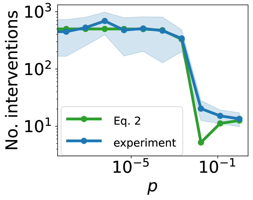
(a)

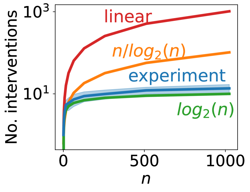
(b)

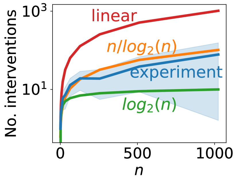
(c)

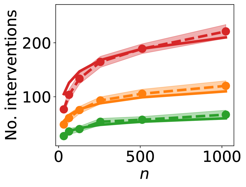
(d)

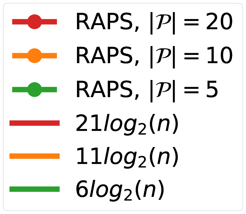
Figure 7: (a) Comparison between eq. 2 from theorem 6.1 and the experimental number of interventions of algorithm 1 on Erdős-Rényi random DAGs. (b-c) The results of running raps on Erdős-Rényi random DAGs with large and small $p$. (d) Results of running algorithm 2 to discover multiple parent nodes.

H.1 Algorithmic Aspect

In this subsection we ignore the statistical aspect of finding the set of parent nodes and assume that each intervention gives us perfect information about the descendants of the intervened on node as well as whether that node is an ancestor of a parent node.

Firstly, we confirm that the eq. 2 could be used to compute the expected number of interventions required to discover the parent node in fig. 7(a). In this experiment we generate Erdős-Rényi random DAG as described in section 6.2.1 with different values of $p$ and for each such DAG compute the expected number of interventions as predicted in eq. 2, as well as perform 20 independent runs on the same graph of algorithm 1. The average over those 20 runs and the standard deviation are shown as the line and the shaded area, respectively, similar to the other figures. For this experiment we set the number of nodes in all graphs $n=1000$. Notice also that eq. 2 matches the lower bound in theorem G.1, thus in fig. 7(a) we show that the performance of our algorithm matches the performance of the best possible algorithm.

Secondly, in fig. 7(b) we confirm the result of corollary 6.5 by showing that when $p=1-\left(\frac{0.5}{\log_{2}(n)-1}\right)^{1/(\log_{2}(n)-1)}$ in Erdős-Rényi random DAG obtained as discussed in section 6.2.1, then the number of interventions required scales as $\mathcal{O}(\log n)$. At the same time, in fig. 7(c) we show that when $p=\frac{\log{n}}{n}$, then the number of interventions scales as $\frac{n}{\log{n}}$.

Additionally, we verify the result of corollary 7.2 in fig. 7(d). On this figure we see that in Erdős-Rényi graphs with $p$ as in the lower bound of corollary 7.2 (with $c_{0}=0.5,c_{1}=1$ and $k=1$) the number of interventions required to discover $\left|\mathcal{P}\right|$ parents grows as $(\left|\mathcal{P}\right|+1)\log(n)$.

H.2 Statistical Aspect

In fig. 8 we present the regret of running our approach raps+UCB and of running just UCB on Erdős-Rényi graphs. For this figure we set $p=\log\log(10)/\log(10)$ and $K=4$. We sample an Erdős-Rényi graph as discussed in section 6.2.1 with $9$ nodes and then add the reward node with a uniformly selected parent. The PCM is such that each node takes the value of a randomly selected parent and uniformly sampled value in the set $[K]$ when there are no parents. The probability of the reward node taking value equal to 1 is the value of its’ parent divided by the maximum value that it can take, $K$. The value of $\delta$ is set to be $0.01$. For UCB algorithm there is only one line since the regrets between the different runs are very close. We can see that while the average regrets of the two approaches are close, raps+UCB has a much bigger variance: it can be much faster than UCB due to quickly finding the parent node or it can not find the parent node during the selected horizon $T=10^{7}$. In our analysis of the results we found that this is due to the large budget $B$ that might be required for some Erdős-Rényi graphs. Note that with our approach it is possible to estimate the number of steps it will take to discover the set of parent nodes and thus one can decide whether or not to use raps before the experiment. Due to the dependence of budget $B$ on $\varepsilon$ and $\Delta$, we explore how the values of these variables depend on the parameters of Erdős-Rényi graphs and the number of parents.

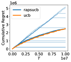
Figure 8: Regret on Erdős-Rényi graph with $p=\log\log(n)/\log(n)$. Bold opaque lines show the mean over 10 runs, other lines show the regrets for each of the 10 runs.

In fig. 9 we present the results of our experiments aimed at studying the behavior of $\varepsilon$ and $\Delta$. For the first figure we vary probability of an edge $p$ and set $n=10$, for the second we vary the number of nodes $n$ and set probability of an edge to be $p=\log\log(n)/\log(n)$, while for the last figure we set $p=\log\log\log(n)/\log\log(n)$ and $n=16$. We can see that for Erdős-Rényi graphs $\varepsilon$ can take small values for substantially high probability and its’ value decreases with the number of nodes $n$.

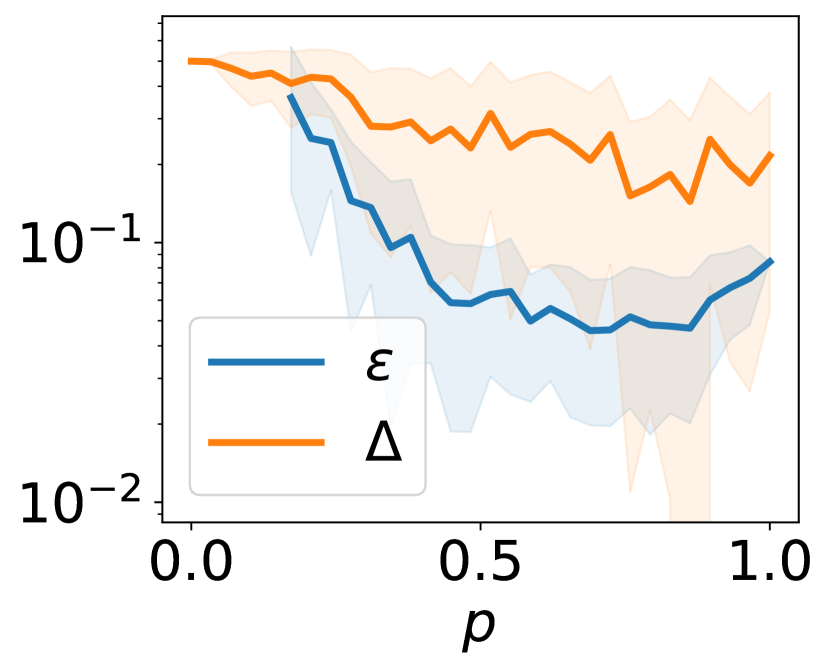
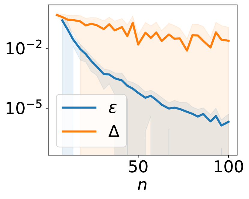
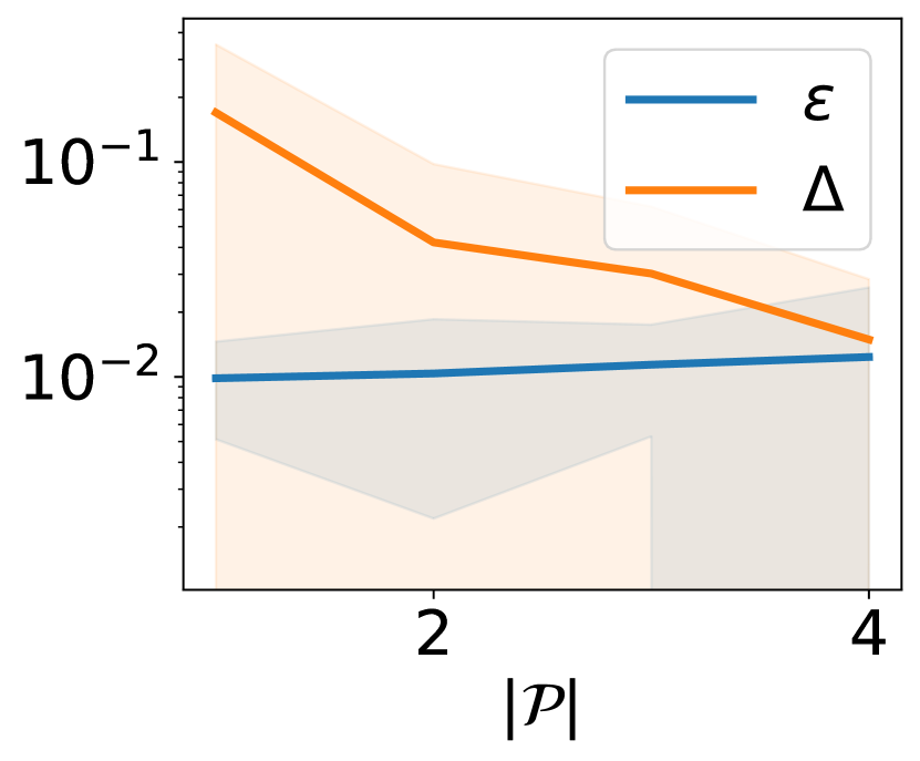
Figure 9: Values of $\varepsilon$ and $\Delta$ for different parameters of Erdős-Rényi graphs and the number of parents.

References

- Abbasi-Yadkori et al. (2011) Yasin Abbasi-Yadkori, Dávid Pál, and Csaba Szepesvári. Improved algorithms for linear stochastic bandits. Advances in neural information processing systems, 24, 2011.
- Agrawal and Goyal (2013) Shipra Agrawal and Navin Goyal. Thompson sampling for contextual bandits with linear payoffs. In International conference on machine learning, pages 127–135. PMLR, 2013.
- Cappé et al. (2013) Olivier Cappé, Aurélien Garivier, Odalric-Ambrym Maillard, Rémi Munos, and Gilles Stoltz. Kullback-leibler upper confidence bounds for optimal sequential allocation. The Annals of Statistics, pages 1516–1541, 2013.
- De Kroon et al. (2022) Arnoud De Kroon, Joris Mooij, and Danielle Belgrave. Causal bandits without prior knowledge using separating sets. In Conference on Causal Learning and Reasoning, pages 407–427. PMLR, 2022.
- Greenewald et al. (2019) Kristjan Greenewald, Dmitriy Katz, Karthikeyan Shanmugam, Sara Magliacane, Murat Kocaoglu, Enric Boix Adsera, and Guy Bresler. Sample efficient active learning of causal trees. Advances in Neural Information Processing Systems, 32, 2019.
- Harris et al. (2020) Charles R. Harris, K. Jarrod Millman, Stéfan J. van der Walt, Ralf Gommers, Pauli Virtanen, David Cournapeau, Eric Wieser, Julian Taylor, Sebastian Berg, Nathaniel J. Smith, Robert Kern, Matti Picus, Stephan Hoyer, Marten H. van Kerkwijk, Matthew Brett, Allan Haldane, Jaime Fernández del Río, Mark Wiebe, Pearu Peterson, Pierre Gérard-Marchant, Kevin Sheppard, Tyler Reddy, Warren Weckesser, Hameer Abbasi, Christoph Gohlke, and Travis E. Oliphant. Array programming with NumPy. Nature, 585(7825):357–362, September 2020. doi: 10.1038/s41586-020-2649-2. URL https://doi.org/10.1038/s41586-020-2649-2.
- Hauser and Bühlmann (2014) Alain Hauser and Peter Bühlmann. Two optimal strategies for active learning of causal models from interventional data. International Journal of Approximate Reasoning, 55(4):926–939, 2014.
- Heckel et al. (2019) Reinhard Heckel, Nihar B Shah, Kannan Ramchandran, and Martin J Wainwright. Active ranking from pairwise comparisons and when parametric assumptions do not help. The Annals of Statistics, 47(6):3099–3126, 2019.
- Hu et al. (2014) Huining Hu, Zhentao Li, and Adrian R Vetta. Randomized experimental design for causal graph discovery. Advances in neural information processing systems, 27, 2014.
- Hunter (2007) J. D. Hunter. Matplotlib: A 2d graphics environment. Computing in Science & Engineering, 9(3):90–95, 2007. doi: 10.1109/MCSE.2007.55.
- Huo and Fu (2017) Xiaoguang Huo and Feng Fu. Risk-aware multi-armed bandit problem with application to portfolio selection. Royal Society open science, 4(11):171377, 2017.
- Jones (1994) Charles H Jones. Generalized hockey stick identities and iv-dimensional blockwalking. 1994.
- Lattimore et al. (2016) Finnian Lattimore, Tor Lattimore, and Mark D Reid. Causal bandits: Learning good interventions via causal inference. Advances in Neural Information Processing Systems, 29, 2016.
- Lattimore and Szepesvári (2020) Tor Lattimore and Csaba Szepesvári. Bandit algorithms. Cambridge University Press, 2020.
- Lee and Bareinboim (2018) Sanghack Lee and Elias Bareinboim. Structural causal bandits: where to intervene? Advances in Neural Information Processing Systems, 31, 2018.
- Liu et al. (2020) Siqi Liu, Kay Choong See, Kee Yuan Ngiam, Leo Anthony Celi, Xingzhi Sun, Mengling Feng, et al. Reinforcement learning for clinical decision support in critical care: comprehensive review. Journal of medical Internet research, 22(7):e18477, 2020.
- Lu et al. (2020) Yangyi Lu, Amirhossein Meisami, Ambuj Tewari, and William Yan. Regret analysis of bandit problems with causal background knowledge. In Conference on Uncertainty in Artificial Intelligence, pages 141–150. PMLR, 2020.
- Lu et al. (2021) Yangyi Lu, Amirhossein Meisami, and Ambuj Tewari. Causal bandits with unknown graph structure. Advances in Neural Information Processing Systems, 34:24817–24828, 2021.
- Mokhtarian et al. (2022) Ehsan Mokhtarian, Sina Akbari, Fateme Jamshidi, Jalal Etesami, and Negar Kiyavash. Learning bayesian networks in the presence of structural side information. In Proceedings of the AAAI Conference on Artificial Intelligence, volume 36, pages 7814–7822, 2022.
- Nair et al. (2021) Vineet Nair, Vishakha Patil, and Gaurav Sinha. Budgeted and non-budgeted causal bandits. In International Conference on Artificial Intelligence and Statistics, pages 2017–2025. PMLR, 2021.
- Pearl (2009) Judea Pearl. Causality. Cambridge university press, 2009.
- Sawant et al. (2018) Neela Sawant, Chitti Babu Namballa, Narayanan Sadagopan, and Houssam Nassif. Contextual multi-armed bandits for causal marketing. arXiv preprint arXiv:1810.01859, 2018.
- Sen et al. (2017) Rajat Sen, Karthikeyan Shanmugam, Alexandros G Dimakis, and Sanjay Shakkottai. Identifying best interventions through online importance sampling. In International Conference on Machine Learning, pages 3057–3066. PMLR, 2017.
- Shanmugam et al. (2015) Karthikeyan Shanmugam, Murat Kocaoglu, Alexandros G Dimakis, and Sriram Vishwanath. Learning causal graphs with small interventions. Advances in Neural Information Processing Systems, 28, 2015.
- Silva et al. (2022) Nícollas Silva, Heitor Werneck, Thiago Silva, Adriano CM Pereira, and Leonardo Rocha. Multi-armed bandits in recommendation systems: A survey of the state-of-the-art and future directions. Expert Systems with Applications, 197:116669, 2022.
- Squires et al. (2020) Chandler Squires, Sara Magliacane, Kristjan Greenewald, Dmitriy Katz, Murat Kocaoglu, and Karthikeyan Shanmugam. Active structure learning of causal dags via directed clique trees. Advances in Neural Information Processing Systems, 33:21500–21511, 2020.
- Yao (1977) Andrew Chi-Chin Yao. Probabilistic computations: Toward a unified measure of complexity. In 18th Annual Symposium on Foundations of Computer Science (sfcs 1977), pages 222–227. IEEE Computer Society, 1977.
- Zhang et al. (2022) Jingwen Zhang, Yifang Chen, and Amandeep Singh. Causal bandits: Online decision-making in endogenous settings. arXiv preprint arXiv:2211.08649, 2022.