Distributed Optimization Methods for Multi-Robot Systems: Part II — A Survey

Abstract

Although the field of distributed optimization is well-developed, relevant literature focused on the application of distributed optimization to multi-robot problems is limited. This survey constitutes the second part of a two-part series on distributed optimization applied to multi-robot problems. In this paper, we survey three main classes of distributed optimization algorithms — distributed first-order methods, distributed sequential convex programming methods, and alternating direction method of multipliers (ADMM) methods — focusing on fully-distributed methods that do not require coordination or computation by a central computer. We describe the fundamental structure of each category and note important variations around this structure, designed to address its associated drawbacks. Further, we provide practical implications of noteworthy assumptions made by distributed optimization algorithms, noting the classes of robotics problems suitable for these algorithms. Moreover, we identify important open research challenges in distributed optimization, specifically for robotics problem.

I Introduction

In this paper we survey the literature in distributed optimization, specifically with an eye toward problems in multi-robot coordination. As we demonstrated in the first paper in this two-part series [1], many multi-robot problems can be written as a sum of local objective functions, subject to a union of local constraint functions. Such problems can be solved with a powerful and growing arsenal of distributed optimization algorithms. Distributed optimization consists of multiple computation nodes working together to minimize a common objective function through local computation iterations and network-constrained communication steps, providing both computational and communication benefits by eliminating the need for data aggregation. Distributed optimization is also robust against the failure of individual nodes, as it does not rely on a central computation station, and many distributed optimization algorithms have inherent privacy-preserving properties, keeping the local data, objective function, and constraint function private to each robot, while still allowing for all robots to benefit from one another. Distributed optimization has not yet been widely employed in robotics, and there exist many open opportunities for research in this space, which we highlight in this survey.

Although the field of distributed optimization is well-established in many areas such as computer networking and power systems, problems in robotics have a number of distinguishing features which are not often considered in the major application areas of distributed optimization. Notably, robots move, unlike their analogous counterparts in these other disciplines, which makes their networks time-varying and prone to bandwidth limitations, packet drops, and delays. Robots often use optimization within a receding horizon or model predictive control loop, so fast convergence to an optimal solution is essential in robotics. In addition, optimization problems in robotics are often constrained (e.g., with safety constraints, input constraints, or kino-dynamics constraints in planning problems), and non-convex (for example, simultaneous localization and mapping (SLAM) is a non-convex optimization, as is trajectory planning and state estimation for any nonlinear robot model). Many existing surveys on distributed optimization do not address these unique characteristics of robotics problems.

This survey constitutes the second part of a two-part series on distributed optimization for multi-robot systems. In this survey, we highlight relevant distributed optimization algorithms and note the classes of robotics problems to which these algorithms can be applied. Noting the large body of work in distributed optimization, we categorize distributed optimization algorithms into three broad classes and identify the practical implications of these algorithms for robotics problems, including the challenges arising in the implementation of these algorithms on robotics platforms.

This survey is aimed at robotics researchers, who are interested in research at the intersection of distributed optimization and multi-robot systems, as well as robotics practitioners who want to harness the benefits of distributed optimization algorithms in solving practical robotics problems. In this survey, we limit our discussion to optimization problems over real-valued decision variables. Although discrete optimization problems (i.e., integer programs or mixed integer programs) arise in some robotics applications, these problems are beyond the scope of this survey. However, we note that distributed algorithms for integer and mixed integer problems have been discussed in a number of different works [2, 3, 4]. Further, we limit our discussion to derivative-based methods, in contrast to derivative-free (zeroth-order) distributed optimization algorithms. We note that derivative-free optimization methods have been discussed extensively in [5, 6, 7, 8, 9, 10].

In many robotics applications, such as field robotics, communication with a central computer (or the cloud) might be infeasible, even though each robot can communicate locally with other neighboring robots. Consequently, we focus particularly on distributed optimization algorithms that permit robots to use local robot-to-robot communication to compute an optimal solution, rather than algorithms that require coordination by a central computer. We note that these methods yield a globally optimal solution for convex problems and, in general, a locally optimal solution for non-convex problems, producing the same quality solution that would be obtained if a centralized method were applied. Although many distributed optimization algorithms are not inherently “online,” we note that many of these algorithms can be applied in online problems within the model predictive control (MPC) framework, where a new optimization problem is solved periodically from streaming data. Nevertheless, we highlight a number of distributed optimization algorithms specifically designed for online problems.

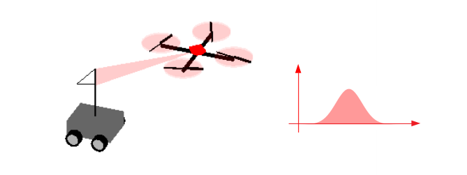
(a) Optimization by one robot yields the solution given only that robot’s observations.

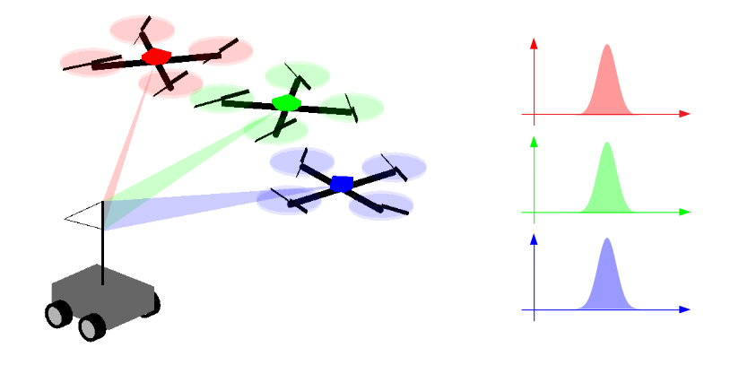
(b) Using distributed optimization, each robot obtains the optimal solution resulting from all robots’ observations.

Figure 1: A motivation for distributed optimization: consider an estimation scenario in which a robot seeks to localize a target given sensor measurements. The robot can compute an optimal solution given only its observations, as represented in (a). By using distributed optimization techniques, each robot in a networked system of robots can compute the optimal solution given all robots’ observations without actually sharing individual sensor models or measurements with one another, as represented in (b).

In this survey, we provide a taxonomy of the different algorithms for performing distributed optimization based on their defining mathematical characteristics. We identify three classes: distributed first-order algorithms, distributed sequential convex programming, and distributed extensions to the alternating direction method of multipliers (ADMM).

Distributed First-Order Algorithms: The most common class of distributed optimization methods is based on the idea of averaging local gradients computed by each computational node to perform an approximate gradient descent update [11], and in this work, we refer to them as Distributed First-Order (DFO) algorithms. DFO algorithms can be further sub-divided into distributed (sub)-gradient descent, distributed gradient tracking, distributed stochastic gradient descent, and distributed dual averaging algorithms, with each sub-category differing from the others based on the order of the update steps and the nature of the gradients used. In general, DFO algorithms utilize a consensus procedure to achieve agreement between the robots on a common solution for the optimization problem. A number of DFO algorithms are amenable to robotics problems with dynamic communication networks (including uni-directional and bi-directional networks) [12, 13] and limited computation resources [14]. However, many DFO algorithms are not suitable for constrained problems.

Distributed Sequential Convex Programming: Sequential Convex Optimization is a common technique in centralized optimization that involves minimizing a sequence of convex approximations to the original (usually non-convex) problem. Under certain conditions, the sequence of sub-problems converges to a local optimum of the original problem. Newton’s method and the Broyden–Fletcher–Goldfarb–Shanno (BFGS) method are common examples. The same concepts are used by a number of distributed optimization algorithms, and we refer to these algorithms as Distributed Sequential Convex Programming methods. Generally, these methods use consensus techniques to construct the convex approximations of the joint objective function. One example is the Network Newton method [15], which uses consensus to approximate the inverse Hessian of the objective to construct a quadratic approximation of the joint problem. The NEXT family of algorithms [16] provides a flexible framework, which can utilize a variety of convex surrogate functions to approximate the joint problem, and is specifically designed to optimize non-convex objective functions. Although many distributed sequential convex programming methods are not suitable for problems with dynamic communication networks, a few distributed sequential convex programming algorithms are amenable to these problems [16].

Alternating Direction Method of Multipliers: The last class of algorithms covered in this paper is based on the alternating direction method of multipliers (ADMM) [17]. ADMM works by minimizing the augmented Lagrangian of the optimization problem using alternating updates to the primal and dual variables [18]. The method is naturally amenable to constrained problems. The original method is distributed, but not in the sense we consider in this survey. Specifically, the original ADMM requires a central computation hub to collect all local primal computations from the nodes to perform a centralized dual update step. ADMM was first modified to remove this requirement for a central node in [19], where it was used for distributed signal processing. The algorithm from [19] has since become known as Consensus ADMM (C-ADMM), although that paper does not introduce this terminology. A number of other distributed variants have been developed to address many unique characteristics, including uni-directional communication networks and limited communication bandwidth [20, 21], which are often present in robotics problems.

I-A Existing Surveys

A number of other recent surveys on distributed optimization exist, and provide useful background when working with the algorithms covered in this survey. Some of these surveys cover applications of distributed optimization in distributed power systems [22], big-data problems [23], and game theory [24], while others focus primarily on first-order methods for problems in multi-agent control [25]. Other articles broadly address distributed first-order optimization methods, including a discussion on the communication-computation trade-offs [26, 27]. Another survey [28] covers exclusively non-convex optimization in both batch and data-streaming contexts, but again only analyzes first-order methods. Finally, [29] covers a wide breadth of distributed optimization algorithms with a variety of assumptions, focusing exclusively on convex optimization problems. Our survey differs from all of these in that it specifically targets applications of distributed optimization to multi-robot problems. As a result, this survey highlights the practical implications of the assumptions made by many distributed optimization algorithms and provides a condensed taxonomic overview of useful methods for these applications. Other useful background material can be found for distributed computation [30] [31], and on multi-robot systems in [32] [33].

I-B Contributions

This survey paper has three primary objectives:

1. Survey the literature across three different classes of distributed optimization algorithms, noting the defining mathematical characteristics of each category.

2. Highlight the practical implications of noteworthy assumptions made by distributed optimization algorithms and the challenges that arise in implementing these algorithms in multi-robot problems.

3. Propose open research problems in distributed optimization for robotics.

I-C Organization

In Section II we introduce mathematical notation and preliminaries, and in Section III we present the general formulation for the distributed optimization problem and describe the general framework shared by distributed optimization algorithms. Sections IV–VI survey the literature in each of the three categories, and provide details for representative algorithms in each category. Section VII provides notable existing applications of distributed optimization in the robotics literature. In Section VIII, we provide practical notes on implementing distributed optimization algorithms in robotics problems. In Section IX, we discuss open research problems in distributed optimization applied to multi-robot systems and robotics in general, and we offer concluding remarks in Section X.

II Notation and Preliminaries

In this section, we introduce the notation used in this paper and provide the definitions of mathematical concepts relevant to the discussion of the distribution optimization algorithms. We denote the gradient of a function ${f:\mathbb{R}^{n}\rightarrow\mathbb{R}}$ as ${\nabla f}$ and its Hessian as ${\nabla^{2}f}$. We denote the vector containing all ones as $\mathbf{1}_{n}$, where $n$ represents the number of elements in the vector. Next, we begin with the definition of stochastic matrices which arise in distributed first-order optimization algorithms.

Definition 1 (Non-negative Matrix).

A matrix ${W\in\mathbb{R}^{n\times n}}$ is referred to as a non-negative matrix if ${w_{ij}\geq 0}$ for all ${i,j\in\{1,\cdots,n\}}$.

Definition 2 (Stochastic Matrix).

A non-negative matrix ${W\in\mathbb{R}^{n\times n}}$ is referred to as a row-stochastic matrix if

$$W\mathbf{1}_{n}=\mathbf{1}_{n},$$ (1)

in other words, the sum of all elements in each row of the matrix equals one. We refer to $W$ as a column-stochastic matrix if

$$\mathbf{1}_{n}^{\top}W=\mathbf{1}_{n}.$$ (2)

Likewise, for a doubly-stochastic matrix $W$,

$$W\mathbf{1}_{n}=\mathbf{1}_{n}\ \text{and}\ \mathbf{1}_{n}^{\top}W=\mathbf{1}_{n}.$$ (3)

Now, we provide the definition of some relevant properties of a sequence.

Definition 3 (Summable Sequence).

A sequence $\{\alpha(k)\}_{k\geq 0}$, with ${k\in\mathbb{N}}$, is a summable sequence if

$$\sum_{k=0}^{\infty}\alpha(k)<\infty.$$ (4)

Definition 4 (Square-Summable Sequence).

A sequence $\{\alpha(k)\}_{k\geq 0}$, with ${k\in\mathbb{N}}$, is a square-summable sequence if

$$\sum_{k=0}^{\infty}\left(\alpha(k)\right)^{2}<\infty.$$ (5)

We discuss some relevant notions of the connectivity of a graph.

Definition 5 (Connectivity of an Undirected Graph).

An undirected graph $\mathcal{G}$ is connected if a path exists between every pair of vertices $(i,j)$ where ${i,j\in\mathcal{V}}$. Note that such a path might traverse other vertices in $\mathcal{G}$.

Definition 6 (Connectivity of a Directed Graph).

A directed graph $\mathcal{G}$ is strongly connected if a directed path exists between every pair of vertices $(i,j)$ where ${i,j\in\mathcal{V}}$. In addition, a directed graph $\mathcal{G}$ is weakly connected if the underlying undirected graph is connected. The underlying undirected graph $\mathcal{G}_{u}$ of a directed graph $\mathcal{G}$ refers to a graph with the same set of vertices as $\mathcal{G}$ and a set of edges obtained by considering each edge in $\mathcal{G}$ as a bi-directional edge. Consequently, every strongly connected directed graph is weakly connected; however, the converse is not true.

In distributed optimization in multi-robot systems, robots perform communication and computation steps to minimize some global objective function. We focus on problems in which the robots’ exchange of information must respect the topology of an underlying distributed communication graph, which could possibly change over time. This communication graph, denoted as $\mathcal{G}(t)=(\mathcal{V}(t),\mathcal{E}(t))$, consists of vertices $\mathcal{V}(t)=\{1,\dots,N\}$ and edges $\mathcal{E}(t)\subseteq\mathcal{V}(t)\times\mathcal{V}(t)$ over which pairwise communication can occur. For undirected graphs, we denote the set of neighbors of robot $i$ as $\mathcal{N}_{i}(t)$. For directed graphs, we refer to the set of robots which can send information to robot $i$ as the set of in-neighbors of robot $i$, denoted by $\mathcal{N}_{i}^{+}(t)$. Likewise, for directed graphs, we refer to the set of robots which can receive information from robot $i$ as the out-neighbors of robot $i$, denoted by $\mathcal{N}_{i}^{-}(t)$.

Definition 7 (Convergence Rate).

Provided that a sequence $\{x^{(k)}\}$ converges to $x^{\star}$, if there exists a positive scalar ${r\in\mathbb{R}}$, with ${r\geq 1}$, and a constant ${\lambda\in\mathbb{R}}$, with ${\lambda>0}$, such that

$$\lim_{k\rightarrow\infty}\frac{\|x^{(k+1)}-x^{\star}\|}{\|x^{(k)}-x^{\star}\|^{r}}=\lambda,$$ (6)

then $r$ defines the order of convergence of the sequence $\{x^{(k)}\}$ to $x^{\star}$. Moreover, the asymptotic error constant is given by $\lambda$.

If ${r=1}$ and ${\lambda=1}$, then $\{x^{(k)}\}$ converges to $x^{\star}$ sub-linearly. However, if ${r=1}$ and ${\lambda<1}$, then $\{x^{(k)}\}$ converges to $x^{\star}$ linearly. Likewise, $\{x^{(k)}\}$ converges to $x^{\star}$ quadratically if ${r=2}$ and cubically if ${r=3}$.

Definition 8 (Synchronous Algorithm).

An algorithm is synchronous if each robot (computational node) has to wait at a predetermined point for a specific message from other robots (computational nodes) before proceeding. In general, the end of an iteration of the algorithm represents the predetermined synchronization point. Conversely, in an asynchronous algorithm, each robot completes each iteration at its own pace, without having to wait at a predetermined point. In other words, at any given time, the number of iterations of an asynchronous algorithm completed by each robot — measured by its local clock — could differ from the number of iterations completed by other robots.

III Problem Formulation

We consider a general distributed optimization problem, which consists of a global objective function expresses as a sum over local component objective functions. Each robot only knows its own objective function. We call such an optimization problem separable. We also consider a set of global constraints consisting of a union over local constraints. Each robot only knows its own local constraints. The resulting optimization problem is given by

$$\begin{split}\min_{x}\>&\sum_{i\in\mathcal{V}}f_{i}(x)\\ \text{subject to }&g_{i}(x)=0\quad\forall i\in\mathcal{V}\\ &h_{i}(x)\leq 0\quad\forall i\in\mathcal{V}\end{split}$$ (7)

where ${x\in\mathbb{R}^{n}}$ denotes the optimization variable and ${f_{i}:\mathbb{R}^{n}\rightarrow\mathbb{R}}$, ${g_{i}:\mathbb{R}^{n}\rightarrow\mathbb{R}}$, and ${h_{i}:\mathbb{R}^{n}\rightarrow\mathbb{R}}$ denote the local objective function, equality constraint function, and inequality constraint function of robot $i$, respectively. The joint optimization problem (7) can be solved locally by each robot if all the robots share their objective and constraint functions with one another. Alternatively, the solution can be computed centrally, if all the local functions are collated at a central station. However, robots typically possess limited computation and communication resources, which precludes each robot from sharing its local functions with other robots, particularly in problems with high-dimensional problem data, such as images, lidar and other perception measurements. Distributed optimization algorithms enable each robot to compute a solution of (7) locally, without sharing its local objective and constraint functions, or its local data. These algorithms assign a copy of the optimization variable to each robot, enabling each robot to update its own copy locally and in parallel with other robots. Moreover, distributed optimization algorithms enforce consensus among the robots for agreement on a common solution of the optimization problem. Consequently, these algorithms solve a reformulation of the optimization problem in (7), given by

$$\begin{split}\min_{\{x_{i},\ \forall i\in\mathcal{V}\}}\>&\sum_{i\in\mathcal{V}}f_{i}(x_{i})\\ \text{subject to }&x_{i}=x_{j}\quad\forall(i,j)\in\mathcal{E}\\ &g_{i}(x_{i})=0\quad\forall i\in\mathcal{V}\\ &h_{i}(x_{i})\leq 0\quad\forall i\in\mathcal{V},\end{split}$$ (8)

where ${x_{i}\in\mathbb{R}^{n}}$ denotes robot $i$’s local copy of the optimization variable. We note that the consensus constraints in (8) ensure agreement among all the robots, with the assumption that the communication graph is connected. Moreover, the consensus constraints are enforced between neighboring robots only, making it compatible with a point-to-point communication network, where robots can only communicate with their one-hop neighbors.

In the following sections, we discuss three broad classes of distributed optimization methods, namely, distributed first-order methods, distributed sequential convex programming methods, and the alternating direction method of multipliers. We note that distributed first-order methods and distributed sequential convex programming methods implicitly enforce the consensus constraints in (8), while the alternating direction method of multipliers enforces these constraints explicitly.

Before proceeding, we highlight the general framework that distributed optimization algorithms share. Distributed optimization algorithms are iterative algorithms in which each robot executes a number of operations over discrete iterations $k=0,1,\dots$ until convergence, where each iteration consists of a communication and computation step. During each communication round, each robot shares a set of its local variables with its neighbors, referred to as its “communicated” variables $\mathcal{Q}_{i}^{(k)}$, which we distinguish from its “internal” variables $\mathcal{P}_{i}^{(k)}$, which are not shared with its neighbors. In general, each algorithm requires initialization of the local variables of each robot, in addition to algorithm-specific parameters, denoted by $\mathcal{R}_{i}^{(k)}$. We note that some algorithms require coordination among the robots for initialization; however, these parameters can be initialized prior to deployment of the robots.

IV Distributed First-Order Algorithms

The optimization problem in (7) (in its unconstrained form) can be solved through gradient descent where the optimization variable is updated using

$$x^{(k+1)}=x^{(k)}-\alpha^{(k)}\nabla f(x^{(k)})$$ (9)

with $\nabla f(x^{(k)})$ denoting the gradient of the objective function at $x^{(k)}$, given by

$$\nabla f(x)=\sum_{i\in\mathcal{V}}\nabla f_{i}(x),$$ (10)

given some scheduled step-size $\alpha^{(k)}$. Inherently, computation of $\nabla f(x^{(k)})$ requires knowledge of the local objective functions or gradients by all robots in the network which is infeasible in many problems.

Distributed First-Order (DFO) algorithms extend the centralized gradient scheme to the distributed setting where robots communicate with one-hop neighbors without knowledge of the local objective functions or gradients of all robots. In DFO methods, each robot updates its local variable using a weighted combination of the local variables or gradients of its neighbors according to the weights specified by a stochastic weighting matrix $W$, allowing for the dispersion of information on the objective function or its gradient through the network. The stochastic matrix $W$ must be compatible with the underlying communication network, with a non-zero element $w_{ij}$ when robot $j$ can send information to robot $i$.

Many DFO algorithms use a doubly-stochastic matrix, a row-stochastic matrix [34], or a column-stochastic matrix, depending on the model of the communication network considered, while other methods use a push-sum approach. In addition, many methods further require symmetry of the doubly-stochastic weighting matrix with ${W=W^{\top}}$. The weight matrix exerts a significant influence on the convergence rates of DFO algorithms, and thus, an appropriate choice of these weights are required for convergence of DFO methods.

The order of the update procedures for the local variables of each robot and the gradient used by each robot in performing its local update procedures differ among DFO algorithms, giving rise to four broad classes of DFO methods: Distributed (Sub)-Gradient Descent and Diffusion Algorithms, Gradient Tracking Algorithms, Distributed Stochastic Gradient Algorithms, and Distributed Dual Averaging. While distributed (sub)-gradient descent algorithms require a decreasing step-size for convergence to an optimal solution, gradient tracking algorithms converge to an optimal solution without this condition. We discuss these distributed methods in the following subsections.

IV-A Distributed (Sub)-Gradient Descent and Diffusion Algorithms

Initialization: $k\leftarrow 0$, ${x_{i}^{(0)}\in\mathbb{R}^{n}}$

Internal variables: $\mathcal{P}_{i}^{(k)}=\emptyset$

Communicated variables: $\mathcal{Q}_{i}^{(k)}=x_{i}^{(k)}$

Parameters: $\mathcal{R}_{i}^{(k)}=(\alpha^{(k)},w_{i})$

do in parallel  $\forall i\in\mathcal{V}$

       Communicate $\mathcal{Q}_{i}^{(k)}$ to all $j\in\mathcal{N}_{i}$

       Receive $\mathcal{Q}_{j}^{(k)}$ from all $j\in\mathcal{N}_{i}$

$$x_{i}^{(k+1)} =\sum_{j\in\mathcal{N}_{i}\cup\{i\}}w_{ij}x_{j}^{(k)}-\alpha^{(k)}\nabla f_{i}(x_{i}^{(k)})$$

$$\alpha^{(k+1)} =\frac{\alpha^{(0)}}{\sqrt{k}}$$

      $k\leftarrow k+1$

while stopping criterion is not satisfied

Algorithm 1 Distributed Gradient Descent (DGD)

Tsitsiklis introduced a model for distributed gradient descent in the 1980s in [35] and [11] (see also [30]). The works of Nedić and Ozdaglar in [14] revisit the problem, marking the beginning of interest in consensus-based frameworks for distributed optimization over the recent decade. This basic model of distributed gradient descent consists of an update term that involves consensus on the optimization variable as well as a step in the direction of the local gradient for each node:

$$x_{i}(k+1)=\sum_{j\in\mathcal{N}_{i}\cup\{i\}}w_{ij}x_{j}(k)-\alpha_{i}(k)\nabla f_{i}(x_{i}(k))$$ (11)

where robot $i$ updates its variable using a weighted combination of its neighbors’ variables determined by the weights $w_{ij}$ with $\alpha_{i}(k)$ denoting its local step-size at iteration $k$.

For convergence to the optimal joint solution, these methods require the step-size to asymptotically decay to zero. As proven in [36], if $\alpha^{(k)}$ is chosen such that the sequence $\{\alpha^{(k)}\}$ is square-summable but not summable, then the optimization variables of all robots converge to the optimal joint solution, given the standard assumptions of a connected network, properly chosen weights, and bounded (sub)-gradients. In contrast, the choice of a constant step-size for all time-steps only guarantees convergence of each robot’s iterates to a neighborhood of the optimal joint solution.

Algorithm 1 summarizes the update step for the distributed gradient descent method in [14] with the step-size ${\alpha^{(k+1)}=\frac{\alpha^{(0)}}{\sqrt{k}}}$, with ${k>0}$.

We note that the update procedure given in (11) requires a doubly-stochastic weighting matrix, which, in general, is incompatible with directed communication networks. Other distributed gradient descent algorithms [37, 38, 39, 40] utilize the push-sum consensus protocol [41] in place of the consensus terms in (11), extending the application of distributed gradient descent schemes to problems with directed communication networks.

In general, with a constant step-size, distributed (sub)-gradient descent algorithms converge at a rate of ${O(1/k)}$ to a neighborhood of the optimal solution in convex problems [42]. With a decreasing step-size, some distributed (sub)-gradient descent algorithms converge to an optimal solution at $O(\log k/k)$ using an accelerated gradient scheme such as the Nesterov gradient method [43].

IV-B Distributed Gradient Tracking Algorithms

Initialization: $k\leftarrow 0$, ${x_{i}^{(0)}\in\mathbb{R}^{n}}$, ${y_{i}^{(0)}=\nabla f_{i}(x_{i}^{(0)})}$

Internal variables: $\mathcal{P}_{i}^{(k)}=\emptyset$

Communicated variables: $\mathcal{Q}_{i}^{(k)}=\left(x_{i}^{(k)},y_{i}^{k}\right)$

Parameters: $\mathcal{R}_{i}^{(k)}=\left(\alpha,w_{i}\right)$

do in parallel  $\forall i\in\mathcal{V}$

       Communicate $\mathcal{Q}_{i}^{(k)}$ to all $j\in\mathcal{N}_{i}$

       Receive $\mathcal{Q}_{j}^{(k)}$ from all $j\in\mathcal{N}_{i}$

$$x_{i}^{(k+1)} =\sum_{j\in\mathcal{N}_{i}\cup\{i\}}w_{ij}x_{j}^{(k)}-\alpha y_{i}^{(k)}$$

$$y_{i}^{(k+1)} =\sum_{j\in\mathcal{N}_{i}\cup\{i\}}w_{ij}y_{j}^{(k)}+\nabla f_{i}(x_{i}^{(k+1)})-\nabla f_{i}(x_{i}^{(k)})$$

      $k\leftarrow k+1$

while stopping criterion is not satisfied

Algorithm 2 DIGing

Although distributed (sub)-gradient descent algorithms converge to an optimal joint solution, the requirement of a square-summable sequence $\{\alpha^{(k)}\}$ — which results in a decaying step-size — reduces the convergence speed of these methods. Gradient tracking methods address this limitation by allowing each robot to utilize the changes in its local gradient between successive iterations as well as a local estimate of the average gradient across all robots in its update procedures, enabling the use of a constant step-size while retaining convergence to the optimal joint solution.

The EXTRA algorithm introduced by Shi et al. in [44] uses a fixed step-size while still achieving exact convergence. EXTRA replaces the gradient term with the difference in the gradients of the previous two iterates. Because the contribution of this gradient difference term decays as the iterates converge to the optimal joint solution, EXTRA does not require the step-size to decay in order to converge to the exact optimal joint solution. EXTRA achieves linear convergence [42], and a variety of gradient tracking algorithms have since offered improvements on its linear rate [45], for convex problems with strongly convex objective functions.

The DIGing algorithm [46, 47], whose update equations are shown in Algorithm 2, is one such similar method that extends the faster convergence properties of EXTRA to the domain of directed and time-varying graphs. DIGing requires communication of two variables, effectively doubling the communication cost per iteration when compared to DGD, but greatly increasing the diversity of communication infrastructure that it can be deployed on.

Many other gradient tracking algorithms involve variations on the variables updated using consensus and the order of the update steps, such as NIDS [48], Exact Diffusion [49, 50], [51], and [52]. These algorithms, which generally require the use of doubly-stochastic weighting matrices, have been extended to problems with row-stochastic or column-stochastic matrices [12, 53, 13, 54] and push-sum consensus [55] for distributed optimization in directed networks. To achieve faster convergence rates, many of these algorithms require each robot to communicate multiple local variables to its neighbors during each communication round. In addition, we note that some of these algorithms require all robots to use the same step-size, which can prove challenging in some situations. Several works offer a synthesis of various gradient tracking methods, noting the similarities between these methods. Under the canonical form proposed in [56, 57], these algorithms and others differ only in the choice of several constant parameters. Jakovetić also provides a unified form for various gradient tracking algorithms in [58]. Some other works consider accelerated variants using Nesterov gradient descent [59, 60, 59, 61]. Gradient tracking algorithms can be considered to be primal-dual methods with an appropriately defined augmented Lagrangian function [46, 62].

In general, gradient tracking algorithms address unconstrained distributed convex optimization problems, but these methods have been extended to non-convex problems [63] and constrained problems using projected gradient descent [64, 65, 66]. Some other methods [67, 68, 69, 70] perform dual-ascent on the dual problem of (7), where the robots compute their local primal variables from the related minimization problem using their dual variables. These methods require doubly-stochastic weighting matrices but allow for time-varying communication networks. In [71], the robots perform a subsequent proximal projection step to obtain solutions which satisfy the problem constraints.

Optimization algorithms that use stochastic gradients have become widely used for problems where evaluating the underlying optimization objectives is a costly procedure, e.g., deep learning. In [72], stochastic gradients are used in place of gradients in the DGD algorithm, and the resulting algorithm is shown to converge.

IV-C Distributed Dual Averaging

Initialization: $k\leftarrow 0$, ${x_{i}^{(0)}\in\mathbb{R}^{n}}$, ${z_{i}^{(0)}=x_{i}^{(0)}}$

Internal variables: $\mathcal{P}_{i}=z_{i}^{(k)}$

Communicated variables: $\mathcal{Q}_{i}^{(k)}=x_{i}^{(k)}$

Parameters:$\mathcal{R}_{i}^{(k)}=\left(\alpha^{(k)},w_{i},\phi(\cdot)\right)$

do in parallel  $\forall i\in\mathcal{V}$

       Communicate $\mathcal{Q}_{i}^{(k)}$ to all $j\in\mathcal{N}_{i}$

       Receive $\mathcal{Q}_{j}^{(k)}$ from all $j\in\mathcal{N}_{i}$

$$z_{i}^{(k+1)} =\sum_{j\in\mathcal{N}_{i}\cup\{i\}}w_{ij}z_{j}^{(k)}+\nabla f_{i}\left(x_{i}^{(k)}\right)$$

$$x_{i}^{(k+1)} =\operatorname*{argmin}_{x\in\mathcal{X}}\left\{x^{\top}z_{i}^{(k+1)}+\frac{1}{\alpha^{(k)}}\phi(x)\right\}$$

      $k\leftarrow k+1$

while stopping criterion is not satisfied

Algorithm 3 Distributed Dual Averaging (DDA)

Dual averaging first posed in [73], and extended in [74], takes a similar approach to distributed (sub)-gradient descent methods in solving the optimization problem in (7), with the added benefit of providing a mechanism for handling problem constraints through a projection step, in like manner as projected (sub)-gradient descent methods. However, the original formulations of the dual averaging method requires knowledge of all components of the objective function or its gradient which is unavailable to all robots. The Distributed Dual Averaging method (DDA) circumvents this limitation by modifying the update equations using a doubly-stochastic weighting matrix to allow for updates of each robot’s variable using its local gradients and a weighted combination of the variables of its neighbors [75].

Similar to distributed (sub)-gradient descent methods, distributed dual averaging requires a sequence of decreasing step-sizes to converge to the optimal solution. Algorithm 3 provides the update equations in the DDA algorithm, along with the projection step which involves a proximal function $\phi(x)$, often defined as $\frac{1}{2}\|x\|_{2}^{2}$. After the projection step, the robot’s variable satisfies the problem constraints described by the constraints set $\mathcal{X}$. Some of the same extensions made to distributed (sub)-gradient descent algorithms have been studied for DDA, including analysis of the algorithm under communication time delays [76] and replacement of the doubly-stochastic weighting matrix with push-sum consensus [77].

V Distributed Sequential Convex Programming

Sequential Convex Programming is a class of optimization methods, typically for non-convex problems, that proceed iteratively by approximating the nonconvex problem with a convex surrogate computed from the current values of the decision variables. This convex surrogate is optimized, and the resulting decision variables are used to compute the convex surrogate for the next iterate. Newton’s method is a classic example of a Sequential Convex Method, in which the convex surrogate is a quadratic approximation of the original objective function. Several methods have been proposed for distributed Sequential Convex Programming, as we survey here.

V-A Approximate Newton Methods

Newton’s method, and its variants, are commonly used for solving convex optimization problems, and provide significant improvements in convergence rate when second-order function information is available [78]. While the distributed gradient descent methods exploit only information on the gradients of the objective function, Newton’s method uses the Hessian of the objective function, providing additional information on the function’s curvature which can improve convergence. To apply Newton’s method to the distributed optimization problem in (7), the Network Newton-$K$ (NN-$K$) algorithm [15] takes a penalty-based approach which introduces consensus between the robots’ variables as components of the objective function. The NN-$K$ method reformulates the constrained form of the distributed problem in (7) as the following unconstrained optimization problem:

$$\min_{\{x_{i},\ \forall i\in\mathcal{V}\}}\>\alpha\sum_{i\in\mathcal{V}}f_{i}(x_{i})+x_{i}^{\top}\left(\sum_{j\in\mathcal{N}\cup\{i\}}\bar{w}_{ij}x_{j}\right)$$ (12)

where $\bar{W}=I-W$, and $\alpha$ is a weighting hyperparameter.

Initialization: $k\leftarrow 0$, ${x_{i}^{(0)}\in\mathbb{R}^{n}}$

Internal variables: $\mathcal{P}_{i}^{(k)}=\left(g_{i}^{(k)},D_{i}^{(k)}\right)$

Communicated variables: $\mathcal{Q}_{i}=\left(x_{i}^{(k)},d_{i}^{(k+1)}\right)$

Parameters: $\mathcal{R}_{i}=\left(\alpha,\epsilon,K,\bar{w}_{i}\right)$

do in parallel  $\forall i\in\mathcal{V}$

      

$$D_{i}^{(k+1)} =\alpha\nabla^{2}f_{i}(x_{i}^{(k)})+2\bar{w}_{ii}I$$

Communicate $x_{i}^{(k)}$ to all $j\in\mathcal{N}_{i}$

$$g_{i}^{(k+1)} =\alpha\nabla f_{i}(x_{i}^{(k)})+\sum_{j\in\mathcal{N}_{i}\cup\{i\}}\bar{w}_{ij}x_{j}^{(k)}$$

$$d_{i}^{(0)} =-\left(D_{i}^{(k+1)}\right)^{-1}g_{i}^{(k+1)}$$

for $p=0$ to $K-1$ do

             Communicate $d_{i}^{(p)}$ to all $j\in\mathcal{N}_{i}$

$$d_{i}^{(p+1)} =\left(D_{i}^{(k+1)}\right)^{-1}\Biggl{[}\bar{w}_{ii}d_{i}^{(p)}-g_{i}^{(k+1)}$$

$$\hskip 80.00012pt-\sum_{j\in\mathcal{N}_{i}\cup\{i\}}\bar{w}_{ij}d_{j}^{(p)}\Biggr{]}$$

       end for

      

$$x_{i}^{(k+1)} =x_{i}^{(k)}+\epsilon\>d_{i}^{(K)}$$

      $k\leftarrow k+1$

while stopping criterion is not satisfied

Algorithm 4 Network Newton-$K$ (NN-$K$)

However, the Newton descent step requires computing the inverse of the joint problem’s Hessian which cannot be directly computed in a distributed manner as its inverse is dense. To allow for distributed computation of the Hessian inverse, NN-$K$ uses the first $K$ terms of the Taylor series expansion ${(I-X)^{-1}=\sum_{j=0}^{\infty}X^{j}}$ to compute the approximate Hessian inverse, as introduced in [79]. Approximation of the Hessian inverse comes at an additional communication cost, and requires an additional $K$ communication rounds per update of the primal variable. Algorithm 4 summarizes the update procedures in the NN-$K$ method in which $\epsilon$ denotes the local step-size for the Newton’s step. Selection of the step-size parameter does not require any coordination between robots. As presented in Algorithm 4, NN-$K$ proceeds through two sets of update equations: an outer set of updates that initializes the Hessian approximation and computes the decision variable update and an inner Hessian approximation update; a communication round precedes the execution of either set of update equations. Increasing $K$, the number of intermediary communication rounds, improves the accuracy of the approximated Hessian inverse at the cost of increasing the communication cost per primal variable update.

A follow-up work optimizes a quadratic approximation of the augmented Lagrangian of the general distributed optimization problem (7) where the primal variable update involves computing a $P$-approximate Hessian inverse to perform a Newton descent step, and the dual variable update uses gradient ascent [80]. The resulting algorithm Exact Second-Order Method (ESOM) provides a faster convergence rate than NN-$K$ at the cost of one additional round of communication for the dual ascent step. Notably, replacing the augmented Lagrangian in the ESOM formulation with its linear approximation results in the EXTRA update equations, showing the relationship between both approaches.

In some cases, computation of the Hessian is impossible because second-order information is not available. Quasi-Newton methods like the Broyden-Flectcher-Goldman-Shanno (BFGS) algorithm approximate the Hessian when it cannot be directly computed. The distributed BFGS (D-BFGS) algorithm [81] replaces the second-order information in the primal update in ESOM with a BFGS approximation (i.e., replaces $D_{i}^{(k)}$ in a call to the Hessian approximation equations in Algorithm 4 with an approximation), and results in essentially a “doubly” approximate Hessian inverse. In [82] the D-BFGS method is extended so that the dual update also uses a distributed Quasi-Newton update scheme, rather than gradient ascent. The resulting primal-dual Quasi-Newton method requires two consecutive iterative rounds of communication doubling the communication overhead per primal variable update compared to its predecessors (NN-$K$, ESOM, and D-BFGS). However, the resulting algorithm is shown by the authors to still converge faster in terms of required communication. In addition, asynchronous variants of the approximate Newton methods have been developed [83].

V-B Convex Surrogate Methods

While the approximate Newton methods in [80, 81, 82] optimize a quadratic approximation of the augmented Lagrangian of (12), other distributed methods allow for more general and direct convex approximations of the distributed optimization problem. These convex approximations generally require the gradient of the joint objective function which is inaccessible to any single robot. In the NEXT family of algorithms [16] dynamic consensus is used to allow each robot to approximate the global gradient, and that gradient is then used to compute a convex approximation of the joint objective function locally. A variety of surrogate functions, $U(\cdot)$, are proposed including linear, quadratic, and block-convex functions, which allows for greater flexibility in tailoring the algorithm to individual applications. Using its surrogate of the joint objective function, each robot updates its local variables iteratively by solving its surrogate for the problem, and then taking a weighted combination of the resulting solution with the solutions of its neighbors. To ensure convergence, NEXT algorithms require a series of decreasing step-sizes, resulting in generally slower convergence rates as well as additional hyperparameter tuning.

Initialization: $k\leftarrow 0$, ${x_{i}^{(0)}\in\mathbb{R}^{n}}$, ${y_{i}^{(0)}=\nabla f_{i}(x_{i}^{(0)})}$, Initialization: ${{\tilde{\pi}}_{i}^{(k+1)}=Ny_{i}^{(0)}-\nabla f_{i}(x_{i}^{(0)})}$

Internal variables: $\mathcal{P}_{i}=\left(x_{i}^{(k)},\tilde{x}_{i}^{(k)},{\tilde{\pi}}_{i}^{(k)}\right)$

Communicated variables: $\mathcal{Q}_{i}^{(k)}=\left(z_{i}^{(k)},y_{i}^{(k)}\right)$

Parameters: $\mathcal{R}_{i}^{(k)}=\left(\alpha^{(k)},w_{i},U(\cdot),\mathcal{K}\right)$

do in parallel  $\forall i\in\mathcal{V}$

      

$${\tilde{x}}_{i}^{(k)} =\operatorname*{argmin}_{x\in\mathcal{K}}\ U\left(x;x_{i}^{(k)},{\tilde{\pi}}_{i}^{(k)}\right)$$

$$z_{i}^{(k)} =x_{i}^{(k)}+\alpha^{(k)}\left({\tilde{x}}_{i}^{(k)}-x_{i}^{(k)}\right)$$

Communicate $\mathcal{Q}_{i}^{(k)}$ to all $j\in\mathcal{N}_{i}$

       Receive $\mathcal{Q}_{j}^{(k)}$ from all $j\in\mathcal{N}_{i}$

$$x_{i}^{(k+1)} =\sum_{j\in\mathcal{N}_{i}\cup\{i\}}w_{ij}z_{j}^{(k)}$$

$$y_{i}^{(k+1)} =\sum_{j\in\mathcal{N}_{i}\cup\{i\}}w_{ij}y_{j}^{(k)}$$

$$\qquad+\left[\nabla f_{i}(x_{i}^{(k+1)})-\nabla f_{i}(x_{i}^{(k)})\right]$$

$${\tilde{\pi}}_{i}^{(k+1)} =N\cdot y_{i}^{(k+1)}-\nabla f_{i}(x_{i}^{(k+1)})$$

      $k\leftarrow k+1$

while stopping criterion is not satisfied

Algorithm 5 NEXT

The SONATA [84] algorithm extends the surrogate function principles of NEXT, and proposes a variety of non-doubly-stochastic weighting schemes that can be used to perform gradient averaging similar to the push-sum protocols. The authors of SONATA also show that several configurations of the algorithm result in already proposed distributed optimization algorithms including Aug-DGM [85], Push-DIG [47], and ADD-OPT [53].

VI Alternating direction method of multipliers

Considering the optimization problem in (8) with only agreement constraints, we have

$$\min_{x_{i}\forall i\in\mathcal{V}} \sum_{i\in\mathcal{V}}f_{i}(x_{i})$$ (13)

subject to $$x_{i}=x_{j}\qquad\forall(i,j)\in\mathcal{E}.$$ (14)

The method of multipliers solves this problem by alternating between minimizing the augmented Lagrangian of the optimization problem with respect to the primal variables $x_{1},\dots,x_{n}$ (the “primal update”) and taking a gradient step to maximize the augmented Lagrangian with respect to the dual (the “dual update”). The augmented Lagrangian of (13) is given by

$$\mathcal{L}_{a}(\mathbf{x},q) =\sum_{i=1}^{N}f_{i}(x_{i})$$ (15)

$$\enspace+\sum_{i=1}^{N}\sum_{j\in\mathcal{N}_{i}}\left(q_{i,j}^{\top}(x_{i}-x_{j})+\frac{\rho}{2}\|x_{i}-x_{j}\|_{2}^{2}\right),$$

where $q_{i,j}$ represents a dual variable for the consensus constraints between robots $i$ and $j$, ${q=\left[q_{i,j}^{\top},\ \forall(i,j)\in\mathcal{E}\right]^{\top}}$, and ${\mathbf{x}=\left[x_{1}^{\top},x_{2}^{\top},\cdots,x_{N}^{\top}\right]^{\top}}$. The parameter ${\rho>0}$ represents a penalty term on the violations of the consensus constraints.

In the alternating direction method of multipliers (ADMM), given the separability of the global objective function, the primal update is executed as successive minimizations over each primal variable (i.e., choose the minimizing $x_{1}$ with all other variables fixed, then choose the minimizing $x_{2}$, and so on). Most ADMM-based approaches do not satisfy our definition of distributed in that either the primal updates take place sequentially rather than in parallel or the dual update requires centralized computation [86, 87, 88]. However, the consensus alternating direction method of multipliers (C-ADMM) provides an ADMM-based optimization method that is fully distributed: the nodes alternate between updating their primal and dual variable and communicating with neighboring nodes [19, 89].

In order to achieve a distributed update of the primal and dual variables, C-ADMM alters the agreement constraints between agents with an existing communication link by introducing auxiliary primal variables in (8) (instead of the constraint $x_{i}=x_{j}$, we have two constraints: $x_{i}=z_{ij}$ and $x_{j}=z_{ij}$). Considering the optimization steps across the entire network, C-ADMM proceeds by optimizing the original primal variables, then the auxiliary primal variables, and then the dual variables, as in the original formulation of ADMM. We can perform minimization with respect to the primal variables and gradient ascent with respect to the dual variables on an augmented Lagrangian that is fully distributed among the robots.

Algorithm 6 summarizes the update procedures for the local primal and dual variables of each agent, where $y_{i}$ represents the dual variable that enforces agreement between robot $i$ and its neighbors. We have incorporated the solution of the auxiliary primal variable update into the update procedure for $x_{i}^{(k+1)}$, noting that the auxiliary primal variable update can be performed implicitly ($z_{ij}^{*}=\frac{1}{2}\left(x_{i}+x_{j}\right)$). The parameter $\rho$ that weights the quadratic terms in $\mathcal{L}_{a}$ is also the step-size in the gradient ascent of the dual variable. We note that the update procedure for $x_{i}^{(k+1)}$ requires solving an optimization problem which might be computationally intensive for certain objective functions. To simplify the update complexity, the optimization can be solved inexactly using a linear approximation of the objective function such as [90, 91, 92] or a quadratic approximation using the Hessian such as DQM [93]. The convergence rate of ADMM methods depends on the value of the penalty parameter $\rho$. Several works discuss effective strategies for optimally selecting $\rho$ [94]. In general, convergence of C-ADMM and its variants is only guaranteed when the dual variables sum to zero, a condition that could be challenging to satisfy in problems with unreliable communication networks. Other distributed ADMM variants which do not require this condition have been developed [95, 96]. However, these methods incur a greater communication overhead to provide robustness in these problems. Gradient tracking algorithms are related to C-ADMM, when the minimization problem in the primal update procedure is solved using a single gradient decent update.

Initialization: $k\leftarrow 0$, ${x_{i}^{(0)}\in\mathbb{R}^{n}}$, ${y_{i}^{(0)}=0}$

Internal variables: $\mathcal{P}_{i}^{(k)}=y_{i}^{(k)}$

Communicated variables: $\mathcal{Q}_{i}^{(k)}=x_{i}^{(k)}$

Parameters: $\mathcal{R}_{i}^{(k)}=\rho$

do in parallel  $\forall i\in\mathcal{V}$

      

$$x_{i}^{(k+1)}=\operatorname*{argmin}_{x_{i}}\Bigg{\{}f_{i}(x_{i})+x_{i}^{\top}y_{i}^{(k)}\cdots$$

$$\hskip 60.00009pt+\rho\sum_{j\in\mathcal{N}_{i}}\left\|x_{i}-\frac{1}{2}\left(x_{i}^{(k)}+x_{j}^{(k)}\right)\right\|^{2}_{2}\Bigg{\}}$$

Communicate $\mathcal{Q}_{i}^{(k)}$ to all $j\in\mathcal{N}_{i}$

       Receive $\mathcal{Q}_{j}^{(k)}$ from all $j\in\mathcal{N}_{i}$

$$y_{i}^{(k+1)} =y_{i}^{(k)}+\rho\sum_{j\in\mathcal{N}_{i}}\left(x_{i}^{(k+1)}-x_{j}^{(k+1)}\right)$$

      $k\leftarrow k+1$

while stopping criterion is not satisfied

Algorithm 6 C-ADMM

C-ADMM, as presented in Algorithm 6, requires each robot to optimize over a local copy of the global decision variable $x$. However, many robotic problems have a fundamental structure that makes maintaining global knowledge at every individual robot unnecessary: each robot’s data relate only to a subset of the global optimization variables, and each agent only requires a subset of the optimization variable for its role. For instance, in distributed SLAM, a memory-efficient solution would require a robot to optimize only over its local map and communicate with other robots only messages of shared interest. Other examples arise in distributed environmental monitoring by multiple robots [97]. The SOVA method [98] leverages the separability of the optimization variable to achieve orders of magnitude improvement in convergence rates, computation, and communication complexity over C-ADMM methods.

In SOVA, each agent only optimizes over variables relevant to its data or role, enabling robotic applications in which agents have minimal access to computation and communication resources. SOVA introduces consistency constraints between each agent’s local optimization variable and its neighbors, mapping the elements of the local optimization variables, given by

$$\Phi_{ij}x_{i}=\Phi_{ji}x_{j}\quad\forall j\in\mathcal{N}_{i},\ \forall i\in\mathcal{V}$$

where $\Phi_{ij}$ and $\Phi_{ji}$ map elements of $x_{i}$ and $x_{j}$ to a common space. C-ADMM represents a special case of SOVA where $\Phi_{ij}$ is always the identity matrix. The update procedures for each agent reduce to the equations given in Algorithm 7.

Initialization: $k\leftarrow 0$, ${x_{i}^{(0)}\in\mathbb{R}^{n_{i}}}$, ${y_{i}^{(0)}=0}$

Internal variables: $\mathcal{P}_{i}^{(k)}=y_{i}^{(k)}$

Communicated variables: $\mathcal{Q}_{i}^{(k)}=x_{i}^{(k)}$

Parameters: $\mathcal{R}_{i}^{(k)}=\rho$

do in parallel  $\forall i\in\mathcal{V}$

      

$$x_{i}^{(k+1)}=\operatorname*{argmin}_{x_{i}}\Bigg{\{}f_{i}(x_{i})+x_{i}^{\top}y_{i}^{(k)}\cdots$$

$$\hskip 20.00003pt+\rho\sum_{j\in\mathcal{N}_{i}}\left\|\Phi_{ij}x_{i}-\frac{1}{2}\left(\Phi_{ij}x_{i}^{(k)}+\Phi_{ji}x_{j}^{(k)}\right)\right\|^{2}_{2}\Bigg{\}}$$

Communicate $\mathcal{Q}_{i}^{(k)}$ to all $j\in\mathcal{N}_{i}$

       Receive $\mathcal{Q}_{j}^{(k)}$ from all $j\in\mathcal{N}_{i}$

$$y_{i}^{(k+1)} =y_{i}^{(k)}+\rho\sum_{j\in\mathcal{N}_{i}}\Phi_{ij}^{\top}\left(\Phi_{ij}x_{i}^{(k)}-\Phi_{ji}x_{j}^{(k)}\right)$$

      $k\leftarrow k+1$

while stopping criterion is not satisfied

Algorithm 7 SOVA

VII Applications of Distributed Optimization in Robotics Literature

In this section, we discuss some existing applications of distributed optimization to robotics problems. To simplify the presentation, we highlight a number of these applications in the following notable problems in robotics: synchronization, localization, mapping, and target tracking; online and deep learning problems; and task assignment, planning, and control. We refer the reader to the first paper in this two-part series [1] for a case study on multi-drone target tracking, which compares solutions using a number of different distributed optimization algorithms.

VII-A Synchronization, Localization, Mapping, and Target Tracking

Distributed optimization algorithms have found notable applications in robot localization from relative measurements [99, 100], including in networks with asynchronous communication [101]. More generally, distributed first-order algorithms have been applied to optimization problems on manifolds, including $SE(3)$ localization [102, 103, 104, 105], synchronization problems [106], and formation control in $SO(3)$ [107, 108]. In pose graph optimization, distributed optimization has been employed through majorization-minimization schemes, which minimize an upper-bound of the objective function [109]; using gradient descent on Riemannian manifolds [110, 111]; and block-coordinate descent [112]. Other pose graph optimization methods have utilized distributed sequential programming algorithms using a quadratic approximation model of the non-convex objective function with Gauss-Seidel updates to enable distributed local computations among the robots [113]. Further, ADMM has been employed in bundle adjustment and pose graph optimization problems, which involve the recovery of the 3D positions and orientations of a map and camera [114, 115, 116]. However, many of these algorithms require a central node for the dual variable updates, making them semi-distributed. Nonetheless, a few fully-distributed ADMM-based algorithms exist for bundle adjustment and cooperative localization problems [117, 118]. Other applications of distributed optimization arise in target tracking [119], signal estimation [19], and parameter estimation in global navigation satellite systems [120].

VII-B Online and Deep Learning Problems

Distributed optimization has been applied in online, dynamic problems, where the objective function of each robot changes with time. In these problems, each robot gains knowledge of its time-varying objective function in an online fashion, after taking an action or decision. A number of distributed first-order algorithms have been designed for these problems [121, 122, 123]. Similarly, DDA has been adapted for online scenarios with static communication graphs [124, 125] and time-varying communication topology [126], [127]. The push-sum variant of dual averaging has also been used for distributed training of deep-learning algorithms, and has been shown to be useful in avoiding pitfalls of other synchronous distributed training frameworks, which face notable challenges in problems with communication deadlocks [128]. In addition, distributed sequential convex programming algorithms have been developed for a number of learning problems where data is distributed, including semi-supervised support vector machines [129], neural network training [130], and clustering [131]. Moreover, ADMM has been applied to online problems, such as estimation and surveillance problems involving wireless sensor networks [132, 133]. ADMM has also be applied to distributed deep learning in robot networks in [134]

VII-C Task Assignment, Planning, and Control

Distributed optimization has been applied to task assignment problems, posed as optimization problems. Some works [135] employ distributed optimization using a distributed simplex method [136] to obtain an optimal assignment of the robots to a desired target formation. Other works employ C-ADMM for distributed task assignment [137]. Further applications of distributed optimization arise in motion planning [138], trajectory tracking problems involving teams of robots using non-linear model predictive control [139], and collaborative manipulation [140, 141], which employ fully-distributed variants of ADMM.

VIII Practical Notes on the Implementation of Distributed Optimization Algorithms

Here, we highlight some relevant issues that arise in the application of distributed optimization algorithms in robotics problems. In particular, we provide alternative distributed algorithms that address these issues, often at the expense of algorithmic performance with respect to convergence.

VIII-1 Selection of a Stochastic Matrix

Distributed first-order algorithms and distributed sequential convex programming algorithms require the specification of a stochastic matrix, which must be compatible with the underlying communication network. As a result, the nature of the communication network available to all robots influences the choice of a stochastic matrix. In general, generating compatible row-stochastic and column-stochastic matrices for directed communication networks does not pose a significant challenge.

To obtain a row-stochastic matrix, each robot assigns a weight to all its in-neighbors such that the sum of all its weights equals one. Conversely, to obtain a column-stochastic matrix, each robot assigns a weight to all its out-neighbors such that the sum of all its weights equals one. In contrast, significant challenges arise when generating doubly-stochastic matrices for directed communication networks. Consequently, in general, algorithms which require doubly-stochastic matrices are unsuitable for problems with directed communication networks.

A number of distributed first-order algorithms allow for the specification of row-stochastic or column-stochastic matrices, making this class of algorithms more amenable to problems with directed communication networks, unlike distributed sequential convex programming algorithms, which generally require the specification of a doubly-stochastic weighting matrix. Further, a number of distributed sequential convex programming algorithms require symmetry of the doubly-stochastic weighting matrix [15, 80, 82, 83], posing an even greater challenge in problems with directed networks.

The specific choice of a doubly-stochastic weighing matrix may vary depending on the assumptions made on what global knowledge is available to the robots on the network. The problem of choosing an optimal weight matrix is discussed thoroughly in [142], in which the authors show that achieving the fastest possible consensus can be posed as a semidefinite program, which a computer with global knowledge of the network can solve efficiently. However, we cannot always assume that global knowledge of the network is available, especially in the case of a time-varying topology. In most cases, Metropolis weights facilitate fast mixing without requiring global knowledge, with the assumption that the communication network is undirected with bi-directional communication links. Each robot can generate its own weight vector after a single communication round with its neighbors. In fact, Metropolis weights perform only slightly sub-optimally compared to centralized optimization-based methods [143]:

$$w_{ij}=\begin{cases}\frac{1}{\max\{|\mathcal{N}_{i}|,|\mathcal{N}_{j}|\}}&j\in\mathcal{N}_{i},\\ 1-\sum_{j^{\prime}\in\mathcal{N}_{i}}w_{ij^{\prime}}&i=j,\\ 0&\text{else}.\end{cases}$$ (16)

Distributed algorithms based on the alternating direction method of multipliers do not require the specification of a stochastic weighting matrix. However, C-ADMM and other distributed variants assume that the communication network between all robots is bi-directional, which makes these algorithms unsuitable for problems with directed communication networks. However, a number of distributed ADMM algorithms for problems with directed communication networks have been developed [144, 20, 145]. Owing to the absence of bi-directional communication links between the robots, these algorithms utilize a dynamic average consensus scheme to update the slack variables at each iteration, which merges information from a robot and its neighbors using a stochastic weighting matrix. However, some of these distributed algorithms require the specification of a doubly-stochastic weighting matrix [145], which introduces notable challenges in problems with directed communication networks, while others allow for the specification of a column-stochastic weighting matrix [20].

VIII-2 Initialization

In general, distributed optimization algorithms allow for an arbitrary initialization of the initial solution of each robot, in convex problems. However, these algorithms often place stringent requirements on the initialization of the algorithms’ parameters. DFO methods require initialization of the step-size and often place conditions on the value of the step-size to guarantee convergence. Some distributed gradient tracking algorithms [47, 51] assume all robots use a common step-size, requiring coordination among all robots. Selecting a common step-size might involve the execution of a consensus procedure by all robots, with additional computation and communication overhead. In algorithms which utilize a fixed step-size, this procedure only needs to be executed once, at the beginning of the optimization algorithm. ADMM and its distributed variants require the selection of a common penalty parameter $\rho$. Consequently, all robots must coordinate among themselves in selecting a value for $\rho$, introducing some challenges, particularly in problems where the convergence rate depends strongly on the value of $\rho$. Initialization of these algorithm-specific parameters have a significant impact on the performance of each algorithm. We refer the reader to the first paper in this series [1], where we empirically study the sensitivity of a number of distributed optimization algorithms to the choice of the algorithm-specific parameters.

VIII-3 Synchronization of the Robots’ Local Clocks

In general, distributed first-order, distributed sequential programming, and distributed ADMM algorithms require the synchronization of the local clock of each robot to a global clock to ensure that the local updates proceed in a synchronous fashion. The global clock keeps track of the current number of iterations executed by all robots. Synchronization of the robots’ local clocks via a distributed scheme presents notable challenges, especially in situations where the time taken by each robot to complete an iteration varies widely. To address these issues, a number of asynchronous distributed first-order algorithms have been developed [146, 147]. Similarly, some asynchronous variants of distributed sequential programming algorithms exist [81, 83], which allow each robot to perform its local updates asynchronously, eliminating the need for synchronization of the local clocks. In addition, a few asynchronous distributed ADMM variants exist [118]. These asynchronous variants are guaranteed to converge to an optimal solution, provided that an integer ${T\in\mathbb{Z}}$ exists such that each robot performs at least one iteration of the algorithm over $T$ time-steps.

VIII-4 Dynamic Communication Networks

In practical situations, the communication network between robots changes over time as the robots move, giving rise to a time-varying communication graph. Networked robots in the real world can also suffer from dropped message packets as well as failed hardware or software components. Generally, distributed first-order optimization algorithms are amenable to problems with dynamic communication networks and are guaranteed to converge to the optimal solution provided that the communication graph is $B$-connected for undirected communication graphs or $B$-strongly connected for directed communication graphs [47], which implies that the union of the communication graphs over $B$ consecutive time-steps is connected or strongly-connected respectively. This property is also referred to as bounded connectivity. This assumption ensures the diffusion of information among all robots. Unlike DFO algorithms, many distributed sequential convex programming algorithms assume the communication network remains static. Nevertheless, a few distributed sequential programming algorithms are amenable to problems with dynamic communication networks [16, 84] and converge to the optimal solution of the problem under the assumption that the sequence of communication graphs is $B$-strongly connected. In general, distributed ADMM algorithms are not amenable to problems with dynamic communication networks. This is an interesting avenue for future research.

IX Open Challenges in Distributed Optimization for Robotics

In this section, we highlight some notable unresolved challenges in the application of distributed optimization to robotics problems. We note, however, that the following discussion does not represent an exhaustive enumeration of these challenges.

IX-A Constrained Robotics Problems

Distributed optimization methods have primarily focused on solving unconstrained convex optimization problems, which constitute a notably limited subset of robotics problems. Generally, robotics problems involve non-convex objectives and constraints, which render these problems not directly amenable to many existing distributed optimization methods. For example, problems in multi-robot motion planning, SLAM, learning, distributed manipulation, and target tracking are often non-convex and/or constrained.

Both DFO methods and C-ADMM methods can be modified for non-convex and constrained problems; however, few examples of practical algorithms or rigorous analyses of performance for such modified algorithms exist in the literature. Specifically, while C-ADMM is naturally amenable to constrained optimization, there are many possible ways to adapt C-ADMM to non-convex objectives, which have yet to be explored. One way to implement C-ADMM for non-convex problems is to solve each primal update step as a non-convex optimization (e.g., through a quasi-Newton method, or interior point method). Another option is to perform successive quadratic approximations in an outer loop, and use C-ADMM to solve each resulting quadratic problem in an inner loop. The trade-off between these two options has not yet been explored in the literature, especially in the context of non-convex problems in robotics.

IX-B Bandwidth-Constrained, Lossy Communication Networks

In many robotics problems, each robot exchanges information with its neighbors over a communication network with a limited communication bandwidth, which effectively limits the size of the message packets that can be transmitted between robots. Moreover, in practical situations, the communication links between robots sometimes fail, resulting in packet losses. However, many distributed optimization methods do not consider communication between agents as an expensive, unreliable resource, given that many of these methods were developed for problems with reliable communication infrastructure (e.g., multi-core computing, or computing in a hard-wired cluster). Information quantization has been extensively employed in many disciplines to allow for efficient exchange of information over bandwidth-constrained networks. Quantization involves encoding the data to be transmitted into a format which utilizes a fewer number of bits, often resulting in lower precision. Transmission of the encoded data incurs a lower communication overhead, enabling each robot to communicate with its neighbors within the bandwidth constraints. A few distributed optimization algorithms have been designed for these problems, including quantized distributed first-order algorithms. Some of these algorithms assume that all robots can communicate with a central node [148, 149], making them unsuitable for a variety of robotics of problems, while others do not make this assumption [150, 151, 152, 153]. In addition, quantized distributed variants of ADMM also exist [21, 154, 155]. Generally, quantization introduces error between each robot’s solution and the optimal solution. However, in some of these algorithms, the quantization error decays during the execution of the algorithms under certain assumptions on the quantizer and the quantization interval [150, 151]. However, quantization in distributed optimization algorithms generally results in slower convergence rates, which poses a challenge in robotics problems where a solution is required rapidly, such as model predictive control problems, highlighting the need for the development of more effective algorithms. Further, only a few distributed optimization algorithms consider problems with lossy communication networks [156, 157, 158].

IX-C Limited Computation Resources

Another valuable direction for future research is in developing algorithms specifically for computationally limited robotic platforms, in which the timeliness of the solution is as important as the solution quality. In general, many distributed optimization methods involve computationally challenging procedures that require significant computational power, especially distributed methods for constrained problems. These methods ignore the significance of computation time, assuming that agents have access to significant computational power. These assumptions often do not hold in robotics problems. Typically, robotics problems unfold over successive time periods with an associated optimization phase at each step of the problem. As such, agents must compute their solutions fast enough to proceed with computing a reasonable solution for the next problem which requires efficient distributed optimization methods. Developing such algorithms specifically for multi-robot systems is an interesting topic for future work.

IX-D Hardware Implementation

Finally, there are very few examples of distributed optimization algorithms implemented and running on multi-robot hardware. This leaves a critical gap in the existing literature, as the ability of these algorithms to run efficiently and robustly on robots has still not be thoroughly proven. As a notable exception, we provide empirical results of a hardare implementation of C-ADMM over XBee radios in the first paper in this series [1].

X Conclusion

Despite the amenability of many robotics problems to distributed optimization, few applications of distributed optimization to multi-robot problems exist. In this work, we have categorized distributed optimization methods into three broad classes—distributed first-order methods, distributed sequential convex programming methods, and the alternating direction method of multipliers (ADMM)—highlighting the distinct mathematical techniques employed by these algorithms. In addition, we have provided practical notes on the implementation of distributed optimization algorithms, with a view towards advancing the application of distributed optimization in robotics. Further, we have identified a number of important open challenges in distributed optimization for robotics, which could be interesting areas for future research. In general, the opportunities for research in distributed optimization for multi-robot systems are plentiful. Distributed optimization provides an appealing unifying framework from which to synthesize solutions for a large variety of problems in multi-robot systems.

References

- [1] O. Shorinwa, T. Halsted, J. Yu, and M. Schwager, “Distributed Optimization Methods for Multi-Robot Systems: Part I — A Tutorial,” 2023.
- [2] I. Prodan, F. Stoican, S. Olaru, C. Stoica, and S.-I. Niculescu, “Mixed-integer programming techniques in distributed mpc problems,” in Distributed Model Predictive Control Made Easy. Springer, 2014, pp. 275–291.
- [3] A. Murray, A. Engelmann, V. Hagenmeyer, and T. Faulwasser, “Hierarchical distributed mixed-integer optimization for reactive power dispatch,” IFAC-PapersOnLine, vol. 51, no. 28, pp. 368–373, 2018.
- [4] A. Testa, A. Rucco, and G. Notarstefano, “Distributed mixed-integer linear programming via cut generation and constraint exchange,” IEEE Transactions on Automatic Control, vol. 65, no. 4, pp. 1456–1467, 2019.
- [5] S. Liu, P.-Y. Chen, B. Kailkhura, G. Zhang, A. O. Hero III, and P. K. Varshney, “A primer on zeroth-order optimization in signal processing and machine learning: Principals, recent advances, and applications,” IEEE Signal Processing Magazine, vol. 37, no. 5, pp. 43–54, 2020.
- [6] D. Hajinezhad, M. Hong, and A. Garcia, “Zeroth order nonconvex multi-agent optimization over networks,” arXiv preprint arXiv:1710.09997, 2017.
- [7] ——, “ZONE: Zeroth-order nonconvex multiagent optimization over networks,” IEEE Transactions on Automatic Control, vol. 64, no. 10, pp. 3995–4010, 2019.
- [8] D. Hajinezhad and M. Hong, “Perturbed proximal primal–dual algorithm for nonconvex nonsmooth optimization,” Mathematical Programming, vol. 176, no. 1-2, pp. 207–245, 2019.
- [9] A. Beznosikov, E. Gorbunov, and A. Gasnikov, “Derivative-free method for composite optimization with applications to decentralized distributed optimization,” IFAC-PapersOnLine, vol. 53, no. 2, pp. 4038–4043, 2020.
- [10] Y. Tang, J. Zhang, and N. Li, “Distributed zero-order algorithms for nonconvex multiagent optimization,” IEEE Transactions on Control of Network Systems, vol. 8, no. 1, pp. 269–281, 2020.
- [11] J. Tsitsiklis, D. Bertsekas, and M. Athans, “Distributed asynchronous deterministic and stochastic gradient optimization algorithms,” IEEE Transactions on Automatic Control, vol. 31, no. 9, pp. 803–812, 1986.
- [12] F. Saadatniaki, R. Xin, and U. A. Khan, “Optimization over time-varying directed graphs with row and column-stochastic matrices,” arXiv preprint arXiv:1810.07393, 2018.
- [13] R. Xin and U. A. Khan, “A linear algorithm for optimization over directed graphs with geometric convergence,” IEEE Control Systems Letters, vol. 2, no. 3, pp. 315–320, 2018.
- [14] A. Nedic and A. Ozdaglar, “Distributed subgradient methods for multi-agent optimization,” IEEE Transactions on Automatic Control, vol. 54, no. 1, pp. 48–61, 2009.
- [15] A. Mokhtari, Q. Ling, and A. Ribeiro, “Network Newton,” Conference Record - Asilomar Conference on Signals, Systems and Computers, vol. 2015-April, pp. 1621–1625, 2015.
- [16] P. Di Lorenzo and G. Scutari, “NEXT: In-network nonconvex optimization,” IEEE Transactions on Signal and Information Processing over Networks, vol. 2, no. 2, pp. 120–136, 2016.
- [17] R. T. Rockafellar, “Monotone operators and the proximal point algorithm,” SIAM journal on control and optimization, vol. 14, no. 5, pp. 877–898, 1976.
- [18] S. Boyd, N. Parikh, E. Chu, B. Peleato, J. Eckstein et al., “Distributed optimization and statistical learning via the alternating direction method of multipliers,” Foundations and Trends® in Machine learning, vol. 3, no. 1, pp. 1–122, 2011.
- [19] G. Mateos, J. A. Bazerque, and G. B. Giannakis, “Distributed sparse linear regression,” IEEE Transactions on Signal Processing, vol. 58, no. 10, pp. 5262–5276, 2010.
- [20] V. Khatana and M. V. Salapaka, “Dc-distadmm: Admm algorithm for contrained distributed optimization over directed graphs,” arXiv preprint arXiv:2003.13742, 2020.
- [21] S. Zhu, M. Hong, and B. Chen, “Quantized consensus admm for multi-agent distributed optimization,” in 2016 IEEE International Conference on Acoustics, Speech and Signal Processing (ICASSP). IEEE, 2016, pp. 4134–4138.
- [22] D. K. Molzahn, F. Dörfler, H. Sandberg, S. H. Low, S. Chakrabarti, R. Baldick, and J. Lavaei, “A survey of distributed optimization and control algorithms for electric power systems,” IEEE Transactions on Smart Grid, vol. 8, no. 6, pp. 2941–2962, 2017.
- [23] G. Scutari and Y. Sun, “Parallel and distributed successive convex approximation methods for big-data optimization,” in Multi-agent Optimization. Springer, 2018, pp. 141–308.
- [24] B. Yang and M. Johansson, “Distributed optimization and games: A tutorial overview,” Networked Control Systems, pp. 109–148, 2010.
- [25] A. Nedić and J. Liu, “Distributed optimization for control,” Annual Review of Control, Robotics, and Autonomous Systems, vol. 1, pp. 77–103, 2018.
- [26] A. Nedić, A. Olshevsky, and M. G. Rabbat, “Network topology and communication-computation tradeoffs in decentralized optimization,” Proceedings of the IEEE, vol. 106, no. 5, pp. 953–976, 2018.
- [27] A. Nedić, “Distributed optimization over networks,” in Multi-agent Optimization. Springer, 2018, pp. 1–84.
- [28] T.-H. Chang, M. Hong, H.-T. Wai, X. Zhang, and S. Lu, “Distributed learning in the nonconvex world: From batch data to streaming and beyond,” IEEE Signal Processing Magazine, vol. 37, no. 3, pp. 26–38, 2020.
- [29] T. Yang, X. Yi, J. Wu, Y. Yuan, D. Wu, Z. Meng, Y. Hong, H. Wang, Z. Lin, and K. H. Johansson, “A survey of distributed optimization,” Annual Reviews in Control, 2019.
- [30] D. P. Bertsekas and J. N. Tsitsiklis, Parallel and distributed computation: numerical methods. Prentice hall Englewood Cliffs, NJ, 1989, vol. 23.
- [31] N. A. Lynch, Distributed algorithms. Elsevier, 1996.
- [32] F. Bullo, J. Cortés, and S. Martínez, Distributed Control of Robotic Networks, ser. Applied Mathematics Series. Princeton University Press, 2009, electronically available at http://coordinationbook.info.
- [33] M. Mesbahi and M. Egerstedt, Graph theoretic methods in multiagent networks. Princeton University Press, 2010, vol. 33.
- [34] V. S. Mai and E. H. Abed, “Distributed optimization over directed graphs with row stochasticity and constraint regularity,” Automatica, vol. 102, pp. 94–104, 2019.
- [35] J. N. Tsitsiklis, “Problems in decentralized decision making and computation.” Massachusetts Inst of Tech Cambridge Lab for Information and Decision Systems, Tech. Rep., 1984.
- [36] I. Lobel and A. Ozdaglar, “Distributed subgradient methods for convex optimization over random networks,” IEEE Transactions on Automatic Control, vol. 56, no. 6, pp. 1291–1306, 2010.
- [37] A. Olshevsky and J. N. Tsitsiklis, “Convergence speed in distributed consensus and averaging,” SIAM Journal on Control and Optimization, vol. 48, no. 1, pp. 33–55, 2009.
- [38] A. Olshevsky, I. C. Paschalidis, and A. Spiridonoff, “Robust asynchronous stochastic gradient-push: asymptotically optimal and network-independent performance for strongly convex functions,” arXiv preprint arXiv:1811.03982, 2018.
- [39] A. Nedić and A. Olshevsky, “Distributed optimization over time-varying directed graphs,” IEEE Transactions on Automatic Control, vol. 60, no. 3, pp. 601–615, 2014.
- [40] F. Bénézit, V. Blondel, P. Thiran, J. Tsitsiklis, and M. Vetterli, “Weighted gossip: Distributed averaging using non-doubly stochastic matrices,” in 2010 ieee international symposium on information theory. IEEE, 2010, pp. 1753–1757.
- [41] D. Kempe, A. Dobra, and J. Gehrke, “Gossip-based computation of aggregate information,” in 44th Annual IEEE Symposium on Foundations of Computer Science. IEEE, 2003, pp. 482–491.
- [42] K. Yuan, Q. Ling, and W. Yin, “On the convergence of decentralized gradient descent,” SIAM Journal on Optimization, vol. 26, no. 3, pp. 1835–1854, 2016.
- [43] D. Jakovetić, J. Xavier, and J. M. Moura, “Fast distributed gradient methods,” IEEE Transactions on Automatic Control, vol. 59, no. 5, pp. 1131–1146, 2014.
- [44] W. Shi, Q. Ling, G. Wu, and W. Yin, “EXTRA: An exact first-order algorithm for decentralized consensus optimization,” SIAM Journal on Optimization, vol. 25, no. 2, pp. 944–966, 2015.
- [45] A. Daneshmand, G. Scutari, and V. Kungurtsev, “Second-order guarantees of distributed gradient algorithms,” arXiv preprint arXiv:1809.08694, 2018.
- [46] A. Nedic, A. Olshevsky, and W. Shi, “Achieving geometric convergence for distributed optimization over time-varying graphs,” SIAM Journal on Optimization, vol. 27, no. 4, pp. 2597–2633, 2017.
- [47] ——, “Achieving geometric convergence for distributed optimization over time-varying graphs,” SIAM Journal on Optimization, vol. 27, no. 4, pp. 2597–2633, 2017.
- [48] Z. Li, W. Shi, and M. Yan, “A decentralized proximal-gradient method with network independent step-sizes and separated convergence rates,” IEEE Transactions on Signal Processing, vol. 67, no. 17, pp. 4494–4506, 2019.
- [49] K. Yuan, B. Ying, X. Zhao, and A. H. Sayed, “Exact diffusion for distributed optimization and learning—part I: Algorithm development,” IEEE Transactions on Signal Processing, vol. 67, no. 3, pp. 708–723, 2018.
- [50] ——, “Exact diffusion for distributed optimization and learning—part II: Convergence analysis,” IEEE Transactions on Signal Processing, vol. 67, no. 3, pp. 724–739, 2018.
- [51] G. Qu and N. Li, “Harnessing smoothness to accelerate distributed optimization,” IEEE Transactions on Control of Network Systems, vol. 5, no. 3, pp. 1245–1260, 2017.
- [52] R. Xin and U. A. Khan, “Distributed heavy-ball: A generalization and acceleration of first-order methods with gradient tracking,” IEEE Transactions on Automatic Control, 2019.
- [53] C. Xi, R. Xin, and U. A. Khan, “ADD-OPT: Accelerated distributed directed optimization,” IEEE Transactions on Automatic Control, vol. 63, no. 5, pp. 1329–1339, 2017.
- [54] C. Xi, V. S. Mai, R. Xin, E. H. Abed, and U. A. Khan, “Linear convergence in optimization over directed graphs with row-stochastic matrices,” IEEE Transactions on Automatic Control, vol. 63, no. 10, pp. 3558–3565, 2018.
- [55] J. Zeng and W. Yin, “ExtraPush for convex smooth decentralized optimization over directed networks,” Journal of Computational Mathematics, vol. 35, no. 4, pp. 383–396, 2017.
- [56] A. Sundararajan, B. Van Scoy, and L. Lessard, “A canonical form for first-order distributed optimization algorithms,” in American Control Conference. IEEE, 2019, pp. 4075–4080.
- [57] ——, “Analysis and design of first-order distributed optimization algorithms over time-varying graphs,” IEEE Transactions on Control of Network Systems, vol. 7, no. 4, pp. 1597–1608, 2020.
- [58] D. Jakovetić, “A unification and generalization of exact distributed first-order methods,” IEEE Transactions on Signal and Information Processing over Networks, vol. 5, no. 1, pp. 31–46, 2018.
- [59] G. Qu and N. Li, “Accelerated distributed nesterov gradient descent,” IEEE Transactions on Automatic Control, 2019.
- [60] R. Xin, D. Jakovetić, and U. A. Khan, “Distributed Nesterov gradient methods over arbitrary graphs,” IEEE Signal Processing Letters, vol. 26, no. 8, pp. 1247–1251, 2019.
- [61] Q. Lü, X. Liao, H. Li, and T. Huang, “A Nesterov-like gradient tracking algorithm for distributed optimization over directed networks,” IEEE Transactions on Systems, Man, and Cybernetics: Systems, 2020.
- [62] F. Mansoori and E. Wei, “A general framework of exact primal-dual first-order algorithms for distributed optimization,” in 2019 IEEE 58th Conference on Decision and Control (CDC). IEEE, 2019, pp. 6386–6391.
- [63] T. Tatarenko and B. Touri, “Non-convex distributed optimization,” IEEE Transactions on Automatic Control, vol. 62, no. 8, pp. 3744–3757, 2017.
- [64] S. S. Ram, A. Nedić, and V. V. Veeravalli, “Distributed stochastic subgradient projection algorithms for convex optimization,” Journal of optimization theory and applications, vol. 147, no. 3, pp. 516–545, 2010.
- [65] P. Bianchi and J. Jakubowicz, “Convergence of a multi-agent projected stochastic gradient algorithm for non-convex optimization,” IEEE transactions on automatic control, vol. 58, no. 2, pp. 391–405, 2012.
- [66] B. Johansson, M. Rabi, and M. Johansson, “A randomized incremental subgradient method for distributed optimization in networked systems,” SIAM Journal on Optimization, vol. 20, no. 3, pp. 1157–1170, 2010.
- [67] M. Maros and J. Jaldén, “PANDA: A dual linearly converging method for distributed optimization over time-varying undirected graphs,” in 2018 IEEE Conference on Decision and Control (CDC). IEEE, 2018, pp. 6520–6525.
- [68] ——, “A geometrically converging dual method for distributed optimization over time-varying graphs,” IEEE Transactions on Automatic Control, 2020.
- [69] ——, “ECO-PANDA: a computationally economic, geometrically converging dual optimization method on time-varying undirected graphs,” in ICASSP 2019-2019 IEEE International Conference on Acoustics, Speech and Signal Processing (ICASSP). IEEE, 2019, pp. 5257–5261.
- [70] K. Seaman, F. Bach, S. Bubeck, Y. T. Lee, and L. Massoulié, “Optimal algorithms for smooth and strongly convex distributed optimization in networks,” in Proceedings of the 34th International Conference on Machine Learning-Volume 70. JMLR. org, 2017, pp. 3027–3036.
- [71] G. Lan, S. Lee, and Y. Zhou, “Communication-efficient algorithms for decentralized and stochastic optimization,” Mathematical Programming, vol. 180, no. 1, pp. 237–284, 2020.
- [72] X. Lian, C. Zhang, H. Zhang, C.-J. Hsieh, W. Zhang, and J. Liu, “Can decentralized algorithms outperform centralized algorithms? a case study for decentralized parallel stochastic gradient descent,” in Proceedings of the 31st International Conference on Neural Information Processing Systems, 2017, pp. 5336–5346.
- [73] Y. Nesterov, “Primal-dual subgradient methods for convex problems,” Mathematical programming, vol. 120, no. 1, pp. 221–259, 2009.
- [74] L. Xiao, “Dual averaging methods for regularized stochastic learning and online optimization,” Journal of Machine Learning Research, vol. 11, no. Oct, pp. 2543–2596, 2010.
- [75] J. C. Duchi, A. Agarwal, and M. J. Wainwright, “Dual averaging for distributed optimization: Convergence analysis and network scaling,” IEEE Transactions on Automatic control, vol. 57, no. 3, pp. 592–606, 2011.
- [76] K. I. Tsianos and M. G. Rabbat, “Distributed consensus and optimization under communication delays,” in 2011 49th Annual Allerton Conference on Communication, Control, and Computing (Allerton). IEEE, 2011, pp. 974–982.
- [77] K. I. Tsianos, S. Lawlor, and M. G. Rabbat, “Push-sum distributed dual averaging for convex optimization,” in 2012 ieee 51st ieee conference on decision and control (cdc). IEEE, 2012, pp. 5453–5458.
- [78] S. Boyd, S. P. Boyd, and L. Vandenberghe, Convex optimization. Cambridge university press, 2004.
- [79] M. Zargham, A. Ribeiro, A. Ozdaglar, and A. Jadbabaie, “Accelerated dual descent for network flow optimization,” IEEE Transactions on Automatic Control, vol. 59, no. 4, pp. 905–920, 2013.
- [80] A. Mokhtari, W. Shi, Q. Ling, and A. Ribeiro, “A decentralized second-order method with exact linear convergence rate for consensus optimization,” IEEE Transactions on Signal and Information Processing over Networks, vol. 2, no. 4, pp. 507–522, 2016.
- [81] M. Eisen, A. Mokhtari, A. Ribeiro, and A. We, “Decentralized Quasi-Newton Methods,” IEEE Transactions on Signal Processing, vol. 65, no. 10, pp. 2613–2628, 2017.
- [82] M. Eisen, A. Mokhtari, and A. Ribeiro, “A Primal-Dual Quasi-Newton Method for Exact Consensus Optimization,” IEEE Transactions on Signal Processing, vol. 67, no. 23, pp. 5983–5997, 2019.
- [83] F. Mansoori and E. Wei, “A fast distributed asynchronous newton-based optimization algorithm,” IEEE Transactions on Automatic Control, vol. 65, no. 7, pp. 2769–2784, 2019.
- [84] Y. Sun and G. Scutari, “Distributed nonconvex optimization for sparse representation,” in 2017 IEEE International Conference on Acoustics, Speech and Signal Processing (ICASSP). IEEE, 2017, pp. 4044–4048.
- [85] J. Xu, S. Zhu, Y. C. Soh, and L. Xie, “Augmented distributed gradient methods for multi-agent optimization under uncoordinated constant stepsizes,” in 2015 54th IEEE Conference on Decision and Control (CDC). IEEE, 2015, pp. 2055–2060.
- [86] B. Houska, J. Frasch, and M. Diehl, “An augmented Lagrangian based algorithm for distributed nonconvex optimization,” SIAM Journal on Optimization, vol. 26, no. 2, pp. 1101–1127, 2016.
- [87] N. Chatzipanagiotis, D. Dentcheva, and M. M. Zavlanos, “An augmented Lagrangian method for distributed optimization,” Mathematical Programming, vol. 152, no. 1-2, pp. 405–434, 2015.
- [88] F. Iutzeler, P. Bianchi, P. Ciblat, and W. Hachem, “Asynchronous distributed optimization using a randomized alternating direction method of multipliers,” in 52nd IEEE conference on decision and control. IEEE, 2013, pp. 3671–3676.
- [89] H. Terelius, U. Topcu, and R. M. Murray, “Decentralized multi-agent optimization via dual decomposition,” IFAC proceedings volumes, vol. 44, no. 1, pp. 11 245–11 251, 2011.
- [90] Q. Ling, W. Shi, G. Wu, and A. Ribeiro, “DLM: Decentralized linearized alternating direction method of multipliers,” IEEE Transactions on Signal Processing, vol. 63, no. 15, pp. 4051–4064, 2015.
- [91] T.-H. Chang, M. Hong, and X. Wang, “Multi-agent distributed optimization via inexact consensus ADMM,” IEEE Transactions on Signal Processing, vol. 63, no. 2, pp. 482–497, 2014.
- [92] F. Farina, A. Garulli, A. Giannitrapani, and G. Notarstefano, “A distributed asynchronous method of multipliers for constrained nonconvex optimization,” Automatica, vol. 103, pp. 243–253, 2019.
- [93] A. Mokhtari, W. Shi, Q. Ling, and A. Ribeiro, “DQM: Decentralized quadratically approximated alternating direction method of multipliers,” IEEE Transactions on Signal Processing, vol. 64, no. 19, pp. 5158–5173, 2016.
- [94] A. Teixeira, E. Ghadimi, I. Shames, H. Sandberg, and M. Johansson, “The admm algorithm for distributed quadratic problems: Parameter selection and constraint preconditioning,” IEEE Transactions on Signal Processing, vol. 64, no. 2, pp. 290–305, 2015.
- [95] D. Meng, M. Fazel, and M. Mesbahi, “Proximal alternating direction method of multipliers for distributed optimization on weighted graphs,” in 2015 54th IEEE Conference on Decision and Control (CDC). IEEE, 2015, pp. 1396–1401.
- [96] A. Makhdoumi and A. Ozdaglar, “Convergence rate of distributed admm over networks,” IEEE Transactions on Automatic Control, vol. 62, no. 10, pp. 5082–5095, 2017.
- [97] M. L. Elwin, R. A. Freeman, and K. M. Lynch, “Distributed environmental monitoring with finite element robots,” IEEE Transactions on Robotics, vol. 36, no. 2, pp. 380–398, 2019.
- [98] O. Shorinwa, T. Halsted, and M. Schwager, “Scalable distributed optimization with separable variables in multi-agent networks,” in 2020 American Control Conference (ACC). IEEE, 2020, pp. 3619–3626.
- [99] V.-L. Dang, B.-S. Le, T.-T. Bui, H.-T. Huynh, and C.-K. Pham, “A decentralized localization scheme for swarm robotics based on coordinate geometry and distributed gradient descent,” in MATEC Web of Conferences, vol. 54. EDP Sciences, 2016, p. 02002.
- [100] N. A. Alwan and A. S. Mahmood, “Distributed gradient descent localization in wireless sensor networks,” Arabian Journal for Science and Engineering, vol. 40, no. 3, pp. 893–899, 2015.
- [101] M. Todescato, A. Carron, R. Carli, and L. Schenato, “Distributed localization from relative noisy measurements: A robust gradient based approach,” in 2015 European Control Conference (ECC). IEEE, 2015, pp. 1914–1919.
- [102] R. Tron and R. Vidal, “Distributed image-based 3-d localization of camera sensor networks,” in Proceedings of the 48h IEEE Conference on Decision and Control (CDC) held jointly with 2009 28th Chinese Control Conference. IEEE, 2009, pp. 901–908.
- [103] ——, “Distributed computer vision algorithms,” IEEE Signal Processing Magazine, vol. 28, no. 3, pp. 32–45, 2011.
- [104] R. Tron, Distributed optimization on manifolds for consensus algorithms and camera network localization. The Johns Hopkins University, 2012.
- [105] R. Tron and R. Vidal, “Distributed 3-d localization of camera sensor networks from 2-d image measurements,” IEEE Transactions on Automatic Control, vol. 59, no. 12, pp. 3325–3340, 2014.
- [106] A. Sarlette and R. Sepulchre, “Consensus optimization on manifolds,” SIAM Journal on Control and Optimization, vol. 48, no. 1, pp. 56–76, 2009.
- [107] K.-K. Oh and H.-S. Ahn, “Formation control and network localization via orientation alignment,” IEEE Transactions on Automatic Control, vol. 59, no. 2, pp. 540–545, 2013.
- [108] ——, “Distributed formation control based on orientation alignment and position estimation,” International Journal of Control, Automation and Systems, vol. 16, no. 3, pp. 1112–1119, 2018.
- [109] T. Fan and T. Murphey, “Majorization minimization methods for distributed pose graph optimization with convergence guarantees,” in 2020 IEEE/RSJ International Conference on Intelligent Robots and Systems (IROS), 2020, pp. 5058–5065.
- [110] Y. Tian, A. Koppel, A. S. Bedi, and J. P. How, “Asynchronous and parallel distributed pose graph optimization,” IEEE Robotics and Automation Letters, vol. 5, no. 4, pp. 5819–5826, 2020.
- [111] J. Knuth and P. Barooah, “Collaborative localization with heterogeneous inter-robot measurements by Riemannian optimization,” in 2013 IEEE International Conference on Robotics and Automation. IEEE, 2013, pp. 1534–1539.
- [112] Y. Tian, K. Khosoussi, and J. P. How, “Block-coordinate descent on the riemannian staircase for certifiably correct distributed rotation and pose synchronization,” arXiv preprint arXiv:1911.03721, 2019.
- [113] S. Choudhary, L. Carlone, C. Nieto, J. Rogers, H. I. Christensen, and F. Dellaert, “Distributed mapping with privacy and communication constraints: Lightweight algorithms and object-based models,” The International Journal of Robotics Research, vol. 36, no. 12, pp. 1286–1311, 2017.
- [114] R. Zhang, S. Zhu, T. Fang, and L. Quan, “Distributed very large scale bundle adjustment by global camera consensus,” in Proceedings of the IEEE International Conference on Computer Vision, 2017, pp. 29–38.
- [115] A. Eriksson, J. Bastian, T.-J. Chin, and M. Isaksson, “A consensus-based framework for distributed bundle adjustment,” in Proceedings of the IEEE Conference on Computer Vision and Pattern Recognition, 2016, pp. 1754–1762.
- [116] S. Choudhary, L. Carlone, H. I. Christensen, and F. Dellaert, “Exactly sparse memory efficient SLAM using the multi-block alternating direction method of multipliers,” in 2015 IEEE/RSJ International Conference on Intelligent Robots and Systems (IROS). IEEE, 2015, pp. 1349–1356.
- [117] K. Natesan Ramamurthy, C.-C. Lin, A. Aravkin, S. Pankanti, and R. Viguier, “Distributed bundle adjustment,” in Proceedings of the IEEE International Conference on Computer Vision Workshops, 2017, pp. 2146–2154.
- [118] S. Kumar, R. Jain, and K. Rajawat, “Asynchronous optimization over heterogeneous networks via consensus ADMM,” IEEE Transactions on Signal and Information Processing over Networks, vol. 3, no. 1, pp. 114–129, 2016.
- [119] O. Shorinwa, J. Yu, T. Halsted, A. Koufos, and M. Schwager, “Distributed multi-target tracking for autonomous vehicle fleets,” in 2020 IEEE International Conference on Robotics and Automation (ICRA). IEEE, 2020, pp. 3495–3501.
- [120] A. Khodabandeh and P. Teunissen, “Distributed least-squares estimation applied to GNSS networks,” Measurement Science and Technology, vol. 30, no. 4, p. 044005, 2019.
- [121] K. Lu, G. Jing, and L. Wang, “Online distributed optimization with strongly pseudoconvex-sum cost functions,” IEEE Transactions on Automatic Control, vol. 65, no. 1, pp. 426–433, 2019.
- [122] S. Shahrampour and A. Jadbabaie, “Distributed online optimization in dynamic environments using mirror descent,” IEEE Transactions on Automatic Control, vol. 63, no. 3, pp. 714–725, 2017.
- [123] Y. Zhang, R. J. Ravier, M. M. Zavlanos, and V. Tarokh, “A distributed online convex optimization algorithm with improved dynamic regret,” in 2019 IEEE 58th Conference on Decision and Control (CDC). IEEE, 2019, pp. 2449–2454.
- [124] S. Hosseini, A. Chapman, and M. Mesbahi, “Online distributed optimization via dual averaging,” in 52nd IEEE Conference on Decision and Control. IEEE, 2013, pp. 1484–1489.
- [125] S. Shahrampour and A. Jadbabaie, “Exponentially fast parameter estimation in networks using distributed dual averaging,” in 52nd IEEE Conference on Decision and Control. IEEE, 2013, pp. 6196–6201.
- [126] S. Hosseini, A. Chapman, and M. Mesbahi, “Online distributed convex optimization on dynamic networks,” IEEE Transactions on Automatic Control, vol. 61, no. 11, pp. 3545–3550, 2016.
- [127] S. Lee, A. Nedić, and M. Raginsky, “Stochastic dual averaging for decentralized online optimization on time-varying communication graphs,” IEEE Transactions on Automatic Control, vol. 62, no. 12, pp. 6407–6414, 2017.
- [128] K. I. Tsianos, S. Lawlor, and M. G. Rabbat, “Consensus-based distributed optimization: Practical issues and applications in large-scale machine learning,” in 2012 50th annual allerton conference on communication, control, and computing (allerton). IEEE, 2012, pp. 1543–1550.
- [129] S. Scardapane, R. Fierimonte, P. Di Lorenzo, M. Panella, and A. Uncini, “Distributed semi-supervised support vector machines,” Neural Networks, vol. 80, pp. 43–52, 2016.
- [130] S. Scardapane and P. Di Lorenzo, “A framework for parallel and distributed training of neural networks,” Neural Networks, vol. 91, pp. 42–54, 2017.
- [131] R. Altilio, P. Di Lorenzo, and M. Panella, “Distributed data clustering over networks,” Pattern Recognition, vol. 93, pp. 603–620, 2019.
- [132] Q. Ling and A. Ribeiro, “Decentralized dynamic optimization through the alternating direction method of multipliers,” IEEE Transactions on Signal Processing, vol. 62, no. 5, pp. 1185–1197, 2013.
- [133] H. F. Xu, Q. Ling, and A. Ribeiro, “Online Learning over a Decentralized Network Through ADMM,” Journal of the Operations Research Society of China, vol. 3, no. 4, pp. 537–562, 2015.
- [134] J. Yu, J. A. Vincent, and M. Schwager, “Dinno: Distributed neural network optimization for multi-robot collaborative learning,” IEEE Robotics and Automation Letters, vol. 7, no. 2, pp. 1896–1903, 2022.
- [135] E. Montijano and A. R. Mosteo, “Efficient multi-robot formations using distributed optimization,” in 53rd IEEE Conference on Decision and Control. IEEE, 2014, pp. 6167–6172.
- [136] M. Bürger, G. Notarstefano, F. Bullo, and F. Allgöwer, “A distributed simplex algorithm for degenerate linear programs and multi-agent assignments,” Automatica, vol. 48, no. 9, pp. 2298–2304, 2012.
- [137] R. Haksar, O. Shorinwa, P. Washington, and M. Schwager, “Consensus-based ADMM for task assignment in multi-robot teams,” in International Symposium on Robotics Research, 2019.
- [138] J. Bento, N. Derbinsky, J. Alonso-Mora, and J. S. Yedidia, “A message-passing algorithm for multi-agent trajectory planning,” in Advances in neural information processing systems, 2013, pp. 521–529.
- [139] L. Ferranti, R. R. Negenborn, T. Keviczky, and J. Alonso-Mora, “Coordination of multiple vessels via distributed nonlinear model predictive control,” in 2018 European Control Conference (ECC). IEEE, 2018, pp. 2523–2528.
- [140] O. Shorinwa and M. Schwager, “Scalable collaborative manipulation with distributed trajectory planning,” in Proceedings of IEEE/RSJ International Conference on Intelligent Robots and Systems. IROS’20, vol. 1. IEEE, 2020, pp. 9108–9115.
- [141] ——, “Distributed contact-implicit trajectory optimization for collaborative manipulation,” in 2021 International Symposium on Multi-Robot and Multi-Agent Systems (MRS). IEEE, 2021, pp. 56–65.
- [142] L. Xiao and S. Boyd, “Fast linear iterations for distributed averaging,” Systems & Control Letters, vol. 53, no. 1, pp. 65–78, 2004.
- [143] S. Jafarizadeh and A. Jamalipour, “Weight optimization for distributed average consensus algorithm in symmetric, CCS & KCS star networks,” arXiv preprint arXiv:1001.4278, 2010.
- [144] V. Khatana and M. V. Salapaka, “D-distadmm: Ao (1/k) distributed admm for distributed optimization in directed graph topologies,” in 2020 59th IEEE Conference on Decision and Control (CDC). IEEE, 2020, pp. 2992–2997.
- [145] K. Rokade and R. K. Kalaimani, “Distributed admm over directed graphs,” arXiv preprint arXiv:2010.10421, 2020.
- [146] X. Lian, W. Zhang, C. Zhang, and J. Liu, “Asynchronous decentralized parallel stochastic gradient descent,” in International Conference on Machine Learning. PMLR, 2018, pp. 3043–3052.
- [147] S. Zheng, Q. Meng, T. Wang, W. Chen, N. Yu, Z.-M. Ma, and T.-Y. Liu, “Asynchronous stochastic gradient descent with delay compensation,” in International Conference on Machine Learning. PMLR, 2017, pp. 4120–4129.
- [148] F. Alimisis, P. Davies, and D. Alistarh, “Communication-efficient distributed optimization with quantized preconditioners,” arXiv preprint arXiv:2102.07214, 2021.
- [149] Y. Yu, J. Wu, and L. Huang, “Double quantization for communication-efficient distributed optimization,” Advances in Neural Information Processing Systems, vol. 32, pp. 4438–4449, 2019.
- [150] Y. Pu, M. N. Zeilinger, and C. N. Jones, “Quantization design for distributed optimization,” IEEE Transactions on Automatic Control, vol. 62, no. 5, pp. 2107–2120, 2016.
- [151] A. Reisizadeh, A. Mokhtari, H. Hassani, and R. Pedarsani, “An exact quantized decentralized gradient descent algorithm,” IEEE Transactions on Signal Processing, vol. 67, no. 19, pp. 4934–4947, 2019.
- [152] C.-S. Lee, N. Michelusi, and G. Scutari, “Finite rate quantized distributed optimization with geometric convergence,” in 2018 52nd Asilomar Conference on Signals, Systems, and Computers. IEEE, 2018, pp. 1876–1880.
- [153] H. Li, S. Liu, Y. C. Soh, and L. Xie, “Event-triggered communication and data rate constraint for distributed optimization of multiagent systems,” IEEE Transactions on Systems, Man, and Cybernetics: Systems, vol. 48, no. 11, pp. 1908–1919, 2017.
- [154] A. Elgabli, J. Park, A. S. Bedi, C. B. Issaid, M. Bennis, and V. Aggarwal, “Q-gadmm: Quantized group admm for communication efficient decentralized machine learning,” IEEE Transactions on Communications, vol. 69, no. 1, pp. 164–181, 2020.
- [155] S. Zhu and B. Chen, “Distributed average consensus with deterministic quantization: An admm approach,” in 2015 IEEE Global Conference on Signal and Information Processing (GlobalSIP). IEEE, 2015, pp. 692–696.
- [156] N. Bastianello, M. Todescato, R. Carli, and L. Schenato, “Distributed optimization over lossy networks via relaxed peaceman-rachford splitting: a robust admm approach,” in 2018 European Control Conference (ECC). IEEE, 2018, pp. 477–482.
- [157] N. Bastianello, R. Carli, L. Schenato, and M. Todescato, “Asynchronous distributed optimization over lossy networks via relaxed admm: Stability and linear convergence,” IEEE Transactions on Automatic Control, vol. 66, no. 6, pp. 2620–2635, 2020.
- [158] N. Bof, R. Carli, G. Notarstefano, L. Schenato, and D. Varagnolo, “Multiagent newton–raphson optimization over lossy networks,” IEEE Transactions on Automatic Control, vol. 64, no. 7, pp. 2983–2990, 2018.