Gravitational Wave from Graviton Bremsstrahlung during Reheating

Abstract

We revisit graviton production via Bremsstrahlung from the decay of the inflaton during inflationary reheating. Using two complementary computational techniques, we first show that such 3-body differential decay rates differ from previously reported results in the literature. We then compute the stochastic gravitational wave (GW) background that forms during the period of reheating, when the inflaton perturbatively decays with the radiative emission of gravitons. By computing the number of relativistic degrees of freedom in terms of $\Delta N_{\text{eff}}$, we constrain the resulting GW energy density from BBN and CMB. Finally, we project current and future GW detector sensitivities in probing such a stochastic GW background, which typically peaks in the GHz to THz ballpark, opening up the opportunity to be detected with microwave cavities and space-based GW detectors.

1 Introduction

The existence of a primordial gravitational wave (GW) background is one of the most crucial predictions of the inflationary scenario of the early universe. Stochastic GWs can have several sources, viz., from the quantum fluctuations during inflation [1, 2, 3, 4] that give rise to tensor perturbations, during preheating [5, 6, 7, 8, 9] when rapid particle production via parametric resonance occurs or from oscillations of cosmic string loops [10, 11, 12, 13], originated from, for example, a spontaneously broken $U(1)$ symmetry (gauged or global) or from the standard model (SM) plasma in thermal equilibrium [14, 15, 16]. However, as pointed out in Refs. [17, 18], stochastic GWs of primordial origin can be sourced from the decay of the inflaton. In that case, after the end of inflation, during the era of reheating, the inflaton field can decay into particles of arbitrary spins, depending on the microscopic nature of its interaction. Considering gravitons to emerge as quantum fluctuations over the classical background, they inexorably couple to matter, leading to a graviton production from inflaton decays, similar to the Bremsstrahlung process as considered in Ref. [20]. It is then unavoidable to have inflaton decay as a source of the primordial GW background.

With this motivation, in this work, we revisit the scenario in which the inflaton can interact with bosons or fermions, leading to its perturbative decay during reheating, resulting in the production of a SM radiation bath. Here, we would like to emphasize that inflaton decay via trilinear couplings fully drains the inflaton energy, allowing the Universe to transit into a radiation-domination phase [21]. By considering fluctuations over a flat background, we introduce the dynamical (massless) graviton field of spin 2 that communicates with all other matter fields through the energy-momentum tensor. This eventually leads to 3-body decay of the inflaton, involving a pair of scalars, fermions, or vector bosons, along with the radiative emission of a graviton. In computing the 3-body decay widths, we follow two complementary approaches: $a)$ we explicitly construct the graviton polarization tensors, and $b)$ we utilize the polarization sum and show that our expressions converge in either case, however, differing from previous analyses reported in Refs. [17, 18, 22]. It is then possible to compute the GW energy density from the differential 3-body decay width of the inflaton.

As is well known, in order for Big Bang Nucleosynthesis (BBN) to proceed successfully, the energy budget of the Universe must not comprise a significant amount of extra relativistic species, including GWs. This condition requires that the energy fraction of GWs to the SM radiation degrees of freedom (DoF) at that time is not greater than about $\sim 10\%$. Regardless of its origin, the energy density in GW established before BBN acts as radiation, and thus its impact on BBN is fully captured by $\Delta N_{\text{eff}}$, which counts the number of relativistic species. Furthermore, GWs with initial adiabatic conditions leave the same imprint on the CMB as free-streaming dark radiation, and in this case, the limit on the present-day energy density in GWs is $\Omega_{\text{GW}}^{(0)}\,h^{2}<1.3\times 10^{-6}$ [23, 24]. We discuss the impact of the CMB measurement of $\Delta N_{\text{eff}}$ on the GW energy density emitted from the decay of the inflaton, taking into account the evolution of the energy densities during reheating. We compare the predicted spectrum of stochastic GWs with existing and future experiments, finding that the present GW spectrum strongly requires high-frequency GW detectors. Interestingly, we see that such high-frequency GWs could be detected, for example, with resonant cavity detectors [25, 26] or with space-based futuristic GW detectors [27, 28]. We refer to Ref. [29] for a recent review on high-frequency GW searches.

The paper is organized as follows. We present the underlying interaction Lagrangian and present the 2- and 3-body decay rates in Section 2. In Section 3 we calculate the constraints from $\Delta N_{\text{eff}}$ on the GW energy density. The computation of the primordial GW spectrum is presented in Section 4. Finally, we conclude in Section 5. In the appendixes, we present our calculations in detail.

2 The Framework

The underlying interaction Lagrangian for the present set-up can be divided into two parts. One part involving a trilinear interaction between the inflaton $\phi$ and a pair of complex scalar doublets $\varphi$ with 4 DoF (which is the SM Higgs field), a pair of vector-like Dirac fermions $\psi$ with 4 DoF, or a pair of massive vector bosons $V_{\mu}$ with 3 DoF, given by

$$\mathcal{L}_{\text{int}}^{(2)}\supset-\mu\,\phi\,|\varphi|^{2}-y_{\psi}\,\overline{\psi}\,\psi\,\phi-g_{V}\,V_{\mu}\,V^{\mu}\,\phi\,,$$ (2.1)

where the corresponding interaction strengths are parameterized in terms of the couplings $\mu$, $y_{\psi}$, and $g_{V}$, respectively. The superscript $(2)$ denotes interactions that lead to a two-body decay of the inflaton. Also, note that the coupling strength $\mu$ and $g_{V}$ have mass dimension, while the Yukawa interaction strength $y_{\psi}$ is dimensionless. Here, we remain agnostic about the underlying UV-complete Lagrangian and, for simplicity, work with an effective theory.

On the other hand, since we are interested in the unavoidable Bremsstrahlung process involving gravitons, we expand the metric $g_{\mu\nu}$ around Minkowski spacetime: $g_{\mu\nu}\simeq\eta_{\mu\nu}+\frac{2}{M_{P}}\,h_{\mu\nu}$, where $M_{P}$ is the reduced Planck mass. This inevitably leads to gravitational interactions that are described by the Lagrangian [30]

$$\sqrt{-g}\,\mathcal{L}_{\rm int}^{(g)}\supset-\frac{2}{M_{P}}\,h_{\mu\nu}\,T^{\mu\nu},$$ (2.2)

where $h_{\mu\nu}$ refers to the graviton field that appears as a quantum fluctuation on the flat background, and $T_{\mu\nu}$ represents the energy-momentum tensor involving all matter particles involved in the theory. Further, we do not consider any non-minimal coupling between the new fields of the theory and gravity; hence, this is a minimal scenario. All relevant Feynman rules involving the graviton and particles of different spins (0, 1/2, and 1) are elaborated in Appendix A. The interactions appearing in Eqs. (2.1) and (2.2) give rise to 2- and 3-body decays of the inflaton into pairs of $\varphi$, $\psi$, and $V$ in the final state, along with the emission of a massless graviton. After production, gravitons propagate and constitute the stochastic GW background, the spectrum of which we shall compute, considering different spins of the final-state products.

With this setup, we now move on to the discussion of three different decay scenarios, where the inflaton $\phi$ perturbatively decays into either a pair of bosons or a pair of fermions, with graviton radiation, due to the graviton-matter coupling. In the following sections, we discuss three cases individually.

Before proceeding, we would like to comment on the possible non-perturbative preheating [31, 32, 33]. For the bosonic case, due to the trilinear coupling, the daughter particles, i.e. the Higgs bosons, could feature a tachyonic mass $\sim\mu\,\phi$, leading to non-perturbative particle production [21]. However, in our case, the bosonic decay product is the SM Higgs, which has a sizable self-coupling $\lambda\,(\varphi^{\dagger}\varphi)^{2}$ that induces a positive mass term $\sim\lambda\left\langle\varphi^{2}\right\rangle$ (with $\left\langle\varphi^{2}\right\rangle$ being the Higgs variance) once the Higgses are copiously produced. This backreaction counteracts the tachyonic mass and quickly terminates non-perturbative particle production, making preheating less efficient [34]. On the other hand, for the fermionic channel, the Pauli blocking effect implies that only a small fraction of the energy stored in the inflaton field can be transferred non–perturbatively [35]. Thereafter, in our setup, a perturbative treatment could capture the dominant phenomena occurring in the reheating phase. We also mention that in the literature, scenarios such as instant preheating [36] could deplete the inflaton energy more efficiently.

2.1 Decay into Scalars

We start with the inflaton decay into spin-0 states, where the final-state particles are considered to be complex doublet scalars, e.g. the SM Higgs doublet. The 2-body decay rate in this case, following the Lagrangian in Eq. (2.1), is given by

$$\Gamma_{0}^{(0)}=\frac{2\,M}{16\,\pi}\left(\frac{\mu}{M}\right)^{2}\sqrt{1-4\,y^{2}}\,,$$ (2.3)

where $y\equiv m/M$, with $m$ being the mass of the daughter particles (independent of their spin). The factor of 2 appears due to two possible decay channels for the complex scalar doublet in the final state. The subscript represents the spin of the final-state particles, while the superscript $(0)$ denotes the 2-body decay width.

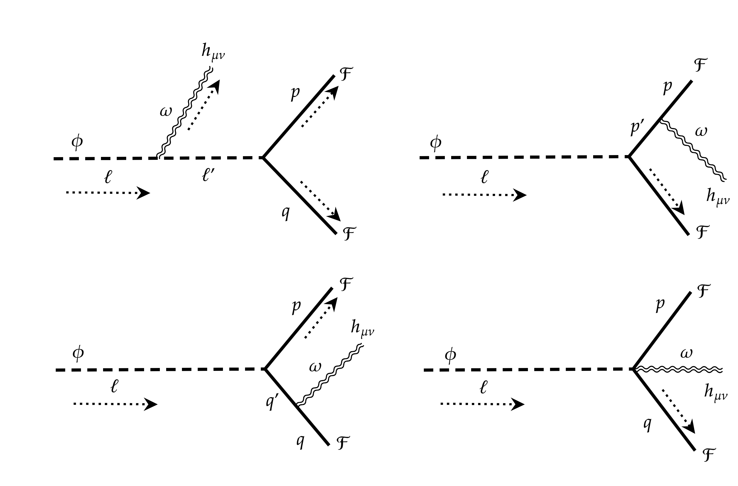
Figure 1: Feynman diagrams for an inflaton decay into a pair of particles $\mathcal{F}$, along with a radiated graviton. Here $\mathcal{F}$ could be a scalar $\varphi$, a fermion $\psi$, or a vector $V$, while $h_{\mu\nu}$ is the graviton tensor field. We denote the incoming and outgoing momenta with dashed arrowheads.

As advocated before, due to the irreducible gravitational interaction (cf. Eq. (2.2)), the final state could also contain a graviton [17], leading to a 3-body decay of $\phi$. The general three-body decay diagrams are shown in Fig. 1, with $l$, $\omega$, $p$, and $q$ denoting the initial and final four-momentum, respectively. Here, we denote any general final state as $\mathcal{F}$, where $\mathcal{F}$ can be a scalar, a fermion, or a gauge boson. The detailed computation of the 3-body decay following two different methodologies, namely the explicit construction of graviton polarization tensors and the polarization sum, is reported in Appendix B. We would like to mention here that, in defining the polarization of massless gravitons, we have taken care of the fact that they satisfy the transverse, traceless, symmetric, and orthonormal conditions in either of the methodologies mentioned above. This results in a different final expression for the 3-body decay width from those derived in Ref. [17]. The differential decay rate for the scalar final state with the emission of a graviton of energy $E_{\omega}$ reads

$$\frac{d\Gamma_{0}^{(1)}}{dE_{\omega}}=\frac{1}{32\,\pi^{3}}\left(\frac{\mu}{M_{P}}\right)^{2}\left[\frac{(1-2x)\,(1-2x+2y^{2})}{4x\,\alpha^{-1}}+\frac{y^{2}\,(y^{2}+2x-1)}{x}\ln\left(\frac{1+\alpha}{1-\alpha}\right)\right],$$ (2.4)

with $x\equiv E_{\omega}/M$ and

$$\alpha\equiv\sqrt{1-\frac{4\,y^{2}}{1-2x}}\,,$$ (2.5)

with a graviton energy spanning the range

$$0<E_{\omega}\leq M\left(\frac{1}{2}-2\,y^{2}\right).$$ (2.6)

Since the differential rate in Eq. (2.4) plays a key role in our subsequent calculation, we would like to make some remarks before proceeding. Note that a graviton could carry at most half of the inflaton energy, which occurs in a limit where the daughter particle mass is zero, namely $y\to 0$. In such a case, the differential decay rate vanishes as the phase space closes. More generally, the differential decay rate should also vanish when $x\to\frac{1}{2}-2\,y^{2}$. We notice that our result differs from that reported in Eq. (7) of Ref. [17].

2.2 Decay into Fermions

Following the second term in Eq. (2.1), we compute the 2-body decay of $\phi$ into a pair of fermions in the final state. In that case, the decay width is given by

$$\Gamma_{1/2}^{(0)}=\frac{y_{\psi}^{2}}{8\pi}\,M\left(1-4\,y^{2}\right)^{3/2}.$$ (2.7)

As before, one can compute the differential rate of the three-body final state involving a pair of $\psi$’s and a graviton in the final state, leading to

$$\frac{d\Gamma_{1/2}^{(1)}}{dE_{\omega}}=\frac{y_{\psi}^{2}}{64\,\pi^{3}}\left(\frac{M}{M_{P}}\right)^{2}\Bigg{[} \frac{1-2x}{x\,\alpha^{-1}}\left[8x\,y^{2}+2x\,(x-1)-8y^{4}-2y^{2}+1\right]$$

$$+\frac{4\,y^{2}\left[(5-8x)\,y^{2}-(x-1)^{2}-4y^{4}\right]}{x}\ln\left(\frac{1+\alpha}{1-\alpha}\right)\Bigg{]},$$ (2.8)

see Appendix B.2 for details. Interestingly, we again find that our expression for the 3-body decay rate differs from those reported in Eq. (8) of Ref. [17] and Eq. (B.1) of Ref. [22].

2.3 Decay into Vectors

For inflaton decays to massive vectors via the trilinear interaction term $\phi\,V_{\mu}V^{\mu}$, the 2-body decay rate is given by

$$\Gamma_{1}^{(0)}=\frac{M}{64\,\pi}\left(\frac{g_{V}}{M}\right)^{2}\,\frac{1-4\,y^{2}+12\,y^{4}}{y^{4}}\,\sqrt{1-4\,y^{2}}\,,$$ (2.9)

while the 3-body differential decay rate reads (see Appendix B.3 for details of the computation)

$$\frac{d\Gamma^{(1)}_{1}}{dE_{\omega}} =\frac{1}{1920\,\pi^{3}\,x\,y^{4}}\left(\frac{g_{V}}{M_{P}}\right)^{2}\bigg{(}\alpha\,\Big{[}360\,(1-2x)\,y^{6}+4\,\left(4x\,\left(23\,x-5\right)+15\right)\,y^{4}$$

$$+2\,(2\,x-1)\,(28\,x\,(14\,x-5)+15)\,y^{2}+(1-2x)^{2}\,\left(4\,x\,\left(2\,x-5\right)+15\right)\Big{]}$$

$$+60\,y^{2}\left[12y^{6}+16(x-1)y^{4}+(5+4x(4x-3))y^{2}-(1-2x)^{2}(1+2x)\right]\ln\left[\frac{1+\alpha}{1-\alpha}\right]\bigg{)}\,.$$ (2.10)

Note that factor $1/y^{4}$ comes from the polarization sum for the massive vector and therefore the massless case cannot be recovered in the limit $y\to 0$. We would like to mention that our results in Eqs. (2.9) and (2.3) differ from the ones reported in Eqs. (4) and (7) of Ref. [18].

3 Gravitational Wave Contribution to $\Delta N_{\text{eff}}$

As we know, to switch to the standard hot Big Bang cosmology after inflation, the inflaton energy must be transferred into SM radiation DoFs, which eventually thermalize and dominate the Universe’s energy budget. This transition process, known as reheating, is typically marked by the equality between the inflaton and radiation energy densities. The reheating process must end before the onset of BBN, which occurs at $T_{\text{BBN}}\simeq 4$ MeV [38, 39, 40, 41, 42]. Now, in order for BBN to proceed successfully, the energy budget of the Universe must not comprise a significant amount of extra relativistic species, including GWs. Regardless of its origin, the energy density established in GW before BBN acts as radiation, and thus its impact on BBN is fully captured in terms of $\Delta N_{\text{eff}}$. Therefore, an excess of the GW energy density around BBN can be restricted by considering the (present and future) bounds on $\Delta N_{\text{eff}}$ from CMB, BBN, and combined. In this section, we discuss our calculations considering that the inflaton $\phi$ oscillates in a simple quadratic potential, which implies that its energy density scales as non-relativistic matter during reheating.

The number of effective neutrinos $N_{\text{eff}}$ is defined from the expression of the radiation energy density in the late universe (at a photon temperature $T_{\Delta N_{\text{eff}}}$) as

$$\rho_{\text{rad}}(T_{\Delta N_{\text{eff}}})=\rho_{\gamma}+\rho_{\nu}+\rho_{\text{GW}}=\left[1+\frac{7}{8}\left(\frac{T_{\nu}}{T_{\gamma}}\right)^{4}N_{\text{eff}}\right]\rho_{\gamma}(T_{\Delta N_{\text{eff}}})\,,$$ (3.1)

where $\rho_{\gamma}$, $\rho_{\nu}$, and $\rho_{\text{GW}}$ correspond to the photon, SM neutrino, and GW energy densities, respectively, with $T_{\nu}/T_{\gamma}=(4/11)^{1/3}$. Note that $T_{\Delta N_{\text{eff}}}$ corresponds to the temperature at which the effective number of neutrinos is evaluated. There are experimental bounds on $\Delta N_{\text{eff}}$ for $T_{\Delta N_{\text{eff}}}=T_{\text{BBN}}$ and $T_{\Delta N_{\text{eff}}}=T_{\text{CMB}}$, where $T_{\text{CMB}}$ is the temperature at which the photons decouple from the thermal plasma. Within the SM, the prediction taking into account the non-instantaneous neutrino decoupling is $N_{\text{eff}}^{\text{SM}}=3.044$ [43, 44, 45, 46, 47, 48, 49, 50, 51], whereas the presence of GWs implies

$$\Delta N_{\text{eff}}\equiv N_{\text{eff}}-N_{\text{eff}}^{\text{SM}}=\frac{8}{7}\left(\frac{11}{4}\right)^{\frac{4}{3}}\frac{\rho_{\text{GW}}(T_{\Delta N_{\text{eff}}})}{\rho_{\gamma}(T_{\Delta N_{\text{eff}}})}=\frac{8}{7}\left(\frac{11}{4}\frac{g_{\star s}(T_{\Delta N_{\text{eff}}})}{g_{\star s}(T_{\text{rh}})}\right)^{\frac{4}{3}}\frac{g_{\star}(T_{\text{rh}})}{2}\frac{\rho_{\text{GW}}(T_{\text{rh}})}{\rho_{R}(T_{\text{rh}})},$$ (3.2)

where

$$\rho_{R}(T) =\frac{\pi^{2}}{30}\,g_{\star}(T)\,T^{4},$$ (3.3)

$$s(T) =\frac{2\pi^{2}}{45}\,g_{\star s}(T)\,T^{3}$$ (3.4)

are the SM radiation energy density and the SM entropy density, with $g_{\star}(T)$ and $g_{\star s}(T)$ the numbers of relativistic degrees of freedom [52].

The evolution of inflaton, SM radiation, and GW energy densities can be tracked using the Boltzmann equations

$$\frac{d\rho_{\phi}}{dt}+3\,H\,\rho_{\phi}=-\left(\Gamma^{(0)}+\Gamma^{(1)}\right)\rho_{\phi}\,,$$ (3.5)

$$\frac{d\rho_{R}}{dt}+4\,H\,\rho_{R}=+\Gamma^{(0)}\,\rho_{\phi}+\int\frac{d\Gamma^{(1)}}{dE_{\omega}}\,\frac{M-E_{\omega}}{M}\,\rho_{\phi}\,dE_{\omega}\,,$$ (3.6)

$$\frac{d\rho_{\text{GW}}}{dt}+4\,H\,\rho_{\text{GW}}=+\int\frac{d\Gamma^{(1)}}{dE_{\omega}}\,\frac{E_{\omega}}{M}\,\rho_{\phi}\,dE_{\omega}\,,$$ (3.7)

where $H$ stands for the Hubble expansion rate given by

$$H^{2}=\frac{\rho_{\phi}+\rho_{R}+\rho_{\text{GW}}}{3\,M_{P}^{2}}\,,$$ (3.8)

while $\Gamma^{(0)}$ and $\Gamma^{(1)}$ are the 2- and 3-body decay widths. The factors $(M-E_{\omega})/M$ and $E_{\omega}/M$ correspond to the fractions of inflaton energy injected into SM radiation and GWs, respectively. It follows that

$$\frac{d(\rho_{\text{GW}}/\rho_{R})}{da}\simeq\frac{1}{a\,H}\,\frac{\rho_{\phi}}{\rho_{R}}\left[\int\frac{d\Gamma^{(1)}}{dE_{\omega}}\,\frac{E_{\omega}}{M}\,dE_{\omega}-\frac{\rho_{\text{GW}}}{\rho_{R}}\,\Gamma^{(0)}\right].$$ (3.9)

This expression can be integrated during reheating, that is, for $a_{\text{max}}\leq a\leq a_{\text{rh}}$, corresponding to photon temperatures $T_{\text{max}}\geq T\geq T_{\text{rh}}$. Note that, in solving Eq. (3.9), we have considered $\rho_{\text{GW}}/\rho_{R}$ as a variable itself, which makes Eq. (3.9) an ordinary first-order differential equation. Importantly, during reheating in which the SM thermal bath is produced and the universe transitions to radiation domination, the bath temperature may rise to a value $T_{\text{max}}$ that exceeds $T_{\text{rh}}$ [53]. The possibility that the maximum temperature of the thermal bath may reach $T_{\text{max}}>T_{\text{rh}}$ before cooling is not apparent if one takes the instantaneous decay approximation for reheating. We note that during reheating

$$\rho_{\phi}(a) =\rho_{\phi}(a_{\text{rh}})\left(\frac{a_{\text{rh}}}{a}\right)^{3},$$ (3.10)

$$T(a) =T_{\text{rh}}\left(\frac{a_{\text{rh}}}{a}\right)^{3/8},$$ (3.11)

as the inflaton is assumed to be non-relativistic and to decay with a constant decay width into SM radiation. The solutions in Eqs. (3.10) and (3.11) can be realized from Eqs. (3.5) and (3.6), considering the fact that during the early stage of reheating (inflaton domination), the decay rate of the inflaton is much smaller than the expansion rate [53], and also utilizing the fact that $\Gamma^{(0)}\gg\Gamma^{(1)}$. We emphasize that the scaling of the SM temperature is due to the fact that the SM radiation is not free, but is sourced by inflaton decays. The end of the reheating corresponds to the moment in which the equality $\rho_{R}(T_{\text{rh}})=\rho_{\phi}(T_{\text{rh}})$ is realized. Additionally, assuming that at the beginning of the reheating, the universe had no SM radiation or GWs, and taking into account that at the end of the reheating $\Gamma^{(0)}\simeq H(T_{\text{rh}})$, Eq. (3.9) admits the analytical solution

$$\frac{\rho_{\text{GW}}(T_{\text{rh}})}{\rho_{R}(T_{\text{rh}})}\simeq\int_{0}^{M/2}\frac{1}{\Gamma^{(0)}}\,\frac{d\Gamma^{(1)}}{dE_{\omega}}\,\frac{E_{\omega}}{M}\,dE_{\omega}\left[1-\left(\frac{T_{\text{rh}}}{T_{\text{max}}}\right)^{8/3}\right].$$ (3.12)

We notice that within the approximation of an instantaneous decay of the inflaton, the expression in the squared brackets reduces to one.

For the different decay channels, in the limit $y\to 0$, one has

$$\frac{\rho_{\text{GW}}(T_{\text{rh}})}{\rho_{R}(T_{\text{rh}})}\simeq\mathcal{C}_{\rho}\,\frac{M^{2}}{\pi^{2}M_{P}^{2}}\left[1-\left(\frac{T_{\text{rh}}}{T_{\text{max}}}\right)^{8/3}\right],$$ (3.13)

where $\mathcal{C}_{\rho}=1/96$ for scalars, $3/128$ for fermions, and $127/1800$ for vectors. Therefore, the corresponding GW contribution to $\Delta N_{\text{eff}}$ is

$$\Delta N_{\text{eff}}\simeq\mathcal{C}_{\Delta N_{\text{eff}}}\left(\frac{M}{M_{P}}\right)^{2}\left[1-\left(\frac{T_{\text{rh}}}{T_{\text{max}}}\right)^{8/3}\right],$$ (3.14)

with $\mathcal{C}_{\Delta N_{\text{eff}}}\simeq 0.01$ for scalars, 0.03 for fermions, and 0.08 for vectors, where we have taken $g_{\star s}(T_{\Delta N_{\text{eff}}})\simeq 10.75$, considering $T_{\Delta N_{\text{eff}}}=T_{\text{BBN}}$. Again, note that in the instantaneous reheating approximation, the square bracket in Eq. (3.14) becomes unity. To avoid jeopardizing the successful predictions from BBN, the reheating temperature must satisfy $T_{\text{rh}}\geq T_{\text{BBN}}$. Furthermore, recent BICEP/Keck measurements have offered a stronger bound (than that of previous Planck results [54]) on the tensor-to-scalar ratio $r<0.035$ [55], implying $T_{\text{rh}}\lesssim 5.5\times 10^{15}$ GeV.

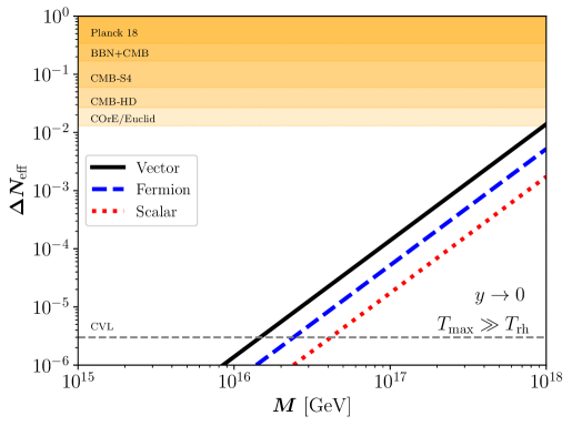
Figure 2: Contribution of GW energy density to $\Delta N_{\text{eff}}$ (cf. Eq. (3.14) with $T_{\text{max}}\gg T_{\text{rh}}$), where the solid black, dashed blue, and dot-dashed red slanted straight lines correspond to scalar, fermion, and vector boson final states. We show the present limits from PLANCK [54], CMB+BBN combined [56], and future limits from CMB-S4 [57], CMB-HD [58], COrE [59]/ Euclid [60], and also hypothetical CVL experiment [61], from top to bottom.

Within the framework of $\Lambda$CDM, Planck legacy data produces $N_{\text{eff}}=2.99\pm 0.34$ at 95% CL [54]. Once the baryon acoustic oscillation (BAO) data are included, the measurement becomes more stringent: $N_{\text{eff}}=2.99\pm 0.17$ at 1$\sigma$ CL. The upcoming CMB experiments, such as SPT-3G [62] and the Simons Observatory [63], will soon improve Planck’s precision on $N_{\text{eff}}$. In particular, CMB-S4 [57] and CMB-HD [58] will be sensitive to a precision of $\Delta N_{\text{eff}}\sim 0.06$ and $\Delta N_{\text{eff}}\sim 0.027$ at 95% CL, respectively. As calculated in Ref. [56], a combined analysis from BBN and CMB results in $N_{\text{eff}}=2.880\pm 0.144$. The next generation of satellite missions, such as COrE [59] and Euclid [60], shall impose limits at $2\sigma$ on $\Delta N_{\text{eff}}\lesssim 0.013$. Furthermore, as mentioned in Ref. [61], a hypothetical cosmic-variance-limited (CVL) CMB polarization experiment could presumably be reduced to as low as $\Delta N_{\text{eff}}\lesssim 3\times 10^{-6}$, although this does not seem to be an experimentally plausible scenario. Fig. 2 illustrates the constraint from $\Delta N_{\text{eff}}$ following Eq. (3.14), considering $T_{\text{max}}\gg T_{\text{rh}}$. As discussed above, we show the present and future limits of $\Delta N_{\text{eff}}$ on the GW energy density for scenarios in which the graviton decays into a pair of scalars (red dotted line), a pair of Dirac fermions (blue dashed line), or a pair of massive vector bosons (black solid line). As we can see, the impact of GW production on $\Delta N_{\text{eff}}$ through all these channels is very challenging not only for present, but even for the projected experimental sensitivities, unless $M\sim M_{P}$. A large inflaton mass is required to overcome the strong Planck suppression originating from minimal graviton coupling. Note that there is a possibility for experiments such as COrE or Euclid to probe the vector scenario.

4 Gravitational Wave Spectrum

After being produced from inflaton 3-body decays, gravitons would propagate and spread in the whole universe, forming a homogeneous and isotropic stochastic GW background at present, after the attenuation of its energy and amplitude due to cosmic expansion. The primordial GW spectrum at present $\Omega_{\text{GW}}(f)$ for a frequency $f$ is defined by

$$\Omega_{\text{GW}}(f)=\frac{1}{\rho_{c}}\,\frac{d\rho_{\text{GW}}}{d\ln f}=\Omega_{\gamma}^{(0)}\,\frac{d(\rho_{\text{GW}}/\rho_{R})}{d\ln f}=\Omega_{\gamma}^{(0)}\,\frac{g_{\star}(T_{\text{rh}})}{g_{\star}(T_{0})}\left[\frac{g_{\star s}(T_{0})}{g_{\star s}(T_{\text{rh}})}\right]^{4/3}\,\frac{d(\rho_{\text{GW}}(T_{\text{rh}})/\rho_{R}(T_{\text{rh}}))}{d\ln E_{\omega}}\,,$$ (4.1)

where $\rho_{c}$ is the critical energy density, and $\Omega_{\gamma}^{(0)}h^{2}\simeq 2.47\times 10^{-5}$ is the observed photon abundance [54]. Equation (4.1) must be evaluated at an energy

$$E_{\omega}=2\pi\,f\,\frac{a_{0}}{a_{\text{rh}}}=2\pi\,f\,\frac{T_{\text{rh}}}{T_{0}}\left[\frac{g_{\star s}(T_{\text{rh}})}{g_{\star s}(T_{0})}\right]^{1/3},$$ (4.2)

taking into account the redshift of the GW energy between the end of reheating and the present epoch.

From Eq. (3.9), the evolution of the differential ratio of GW to SM radiation energy densities is given by

$$\frac{d}{da}\frac{d(\rho_{\text{GW}}/\rho_{R})}{dE_{\omega}}\simeq\frac{1}{a\,H(a)}\,\frac{\rho_{\phi}(a)}{\rho_{R}(a)}\left[\left.\frac{d\Gamma^{(1)}}{dE^{\prime}_{\omega}}\,\frac{E^{\prime}_{\omega}}{M}\right|_{E^{\prime}_{\omega}=E_{\omega}\frac{a_{\text{rh}}}{a}}-\frac{d(\rho_{\text{GW}}/\rho_{R})}{dE_{\omega}}\,\Gamma^{(0)}\right],$$ (4.3)

where in the source term for GWs the redshift of the graviton energy $E^{\prime}_{\omega}(a)=E_{\omega}\,\frac{a_{\text{rh}}}{a}$ was taken into account. An approximate solution is

$$\frac{d(\rho_{\text{GW}}(T_{\text{rh}})/\rho_{R}(T_{\text{rh}}))}{dE_{\omega}}\simeq\frac{d\Gamma^{(1)}}{dE_{\omega}}\,\frac{E_{\omega}}{M}\,\frac{1}{\Gamma^{(0)}}\left[1-\left(\frac{T_{\text{rh}}}{T_{\text{max}}}\right)^{8/3}\right],$$ (4.4)

where again, within the approximation of an instantaneous decay of the inflaton, the expression in the squared brackets reduces to one. For the inflaton decay into particles with different spins, one has

$$\Omega_{\text{GW}}(f)\simeq\mathcal{C}_{\Omega_{\text{GW}}}\,\frac{T_{\text{rh}}}{5.5\times 10^{15}}\,\frac{M}{M_{P}}\,\frac{f}{10^{12}~{}\text{Hz}}\,,$$ (4.5)

with $\mathcal{C}_{\Omega_{\text{GW}}}\simeq 1.4\times 10^{-8}$ for scalars, $\mathcal{C}_{\Omega_{\text{GW}}}\simeq 2.8\times 10^{-8}$ for fermions, and $\mathcal{C}_{\Omega_{\text{GW}}}\simeq 11.2\times 10^{-8}$ for vectors. The latter expression is valid for frequencies $f$ smaller than

$$f\lesssim\frac{M}{4\pi}\,\frac{T_{0}}{T_{\text{rh}}}\left[\frac{g_{\star s}(T_{0})}{g_{\star s}(T_{\text{rh}})}\right]^{1/3}\simeq 4.1\times 10^{12}\,\left(\frac{M}{M_{P}}\right)\,\left(\frac{5.5\times 10^{15}~{}\text{GeV}}{T_{\text{rh}}}\right)\text{Hz}\,,$$ (4.6)

where we have used $g_{\star s}(T_{0})=3.94$ and $g_{\star s}(T_{\text{rh}})=106.75$.

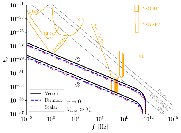
Figure 3: Dimensionless strain $h_{c}$ as a function of the GW frequency $f$, for the two benchmarks (➀ and ➁) described in the text, assuming $T_{\text{max}}\gg T_{\text{rh}}$ and $y\to 0$. The black solid, blue dashed, and red dotted curves correspond to decays into vector, fermion, and scalar final states, respectively. Projected sensitivities from different GW detection experiments are also shown in orange (adapted from Refs. [64, 65]). The gray dashed diagonal lines are CMB bounds on $\Delta N_{\text{eff}}$ from Planck, COrE/Euclid, and a hypothetical CVL experiment, respectively.

Finally, we compute the dimensionless strain defined as [66]

$$h_{c}(f)=\frac{1}{f}\,\sqrt{\frac{3\,H_{0}^{2}\,\Omega_{\text{GW}}(f)}{2\pi^{2}}}=1.26\times 10^{-18}\,\left(\frac{\rm{Hz}}{f}\right)\sqrt{h^{2}\,\Omega_{\text{GW}}(f)}\,,$$ (4.7)

where $H_{0}\equiv H(T_{0})\simeq 1.44\times 10^{-42}$ GeV is the present-day Hubble parameter, and $h=0.674$ [54]. In Fig. 3 we show the dimensionless strain $h_{c}$ as a function of the GWs frequency $f$, for two benchmark points: ➀ $M=M_{P}/10$ and $T_{\text{rh}}=5.5\times 10^{15}$ GeV, and ➁ $M=M_{P}/10^{3}$ and $T_{\text{rh}}=M_{P}/(2\times 10^{4})$. In the same plane, we project the limits from several proposed GW detectors, for example, LISA [67], the Einstein Telescope (ET) [68, 69, 70, 71], the Big Bang Observer (BBO) [72, 73, 74], ultimate DECIGO (uDECIGO) [27, 28], GW-electromagnetic wave conversion in the vacuum (solid) and in a Gaussian beam (GB) (dotted) [75, 64], resonant cavities [25, 26], and the International Axion Observatory (IAXO) [76, 77]. We have projected the $\Delta N_{\text{eff}}$ bounds from Planck, COrE/Euclid and CVL from Fig. 2 as a bound on the GW strain using [66]

$$\int d\left(\ln f\right)\Omega_{\text{GW}}(f)\,h^{2}\leq 5.6\times 10^{-6}\,\Delta N_{\text{eff}}\,.$$ (4.8)

These are shown by the diagonal straight gray lines. As can be inferred from Eq. (4.6), a larger $M/T_{\text{rh}}$ ratio corresponds to a higher frequency, which is also reflected in Fig. 3 curves. As we see, only microwave cavity detectors are capable of probing the high-frequency regime of the GW spectrum. Detectors such as uDECIGO, on the other hand, might be able to reach the lower frequency part of the spectrum.

5 Conclusions

Inflaton 3-body decay is a source of the stochastic gravitational wave (GW) background, due to the inexorable graviton Bremsstrahlung. In this work, we have revisited such three-body decay rates, considering the perturbative coupling of the inflaton with a pair of massive spin-0 bosons, spin-1/2 fermions, and spin-1 vector bosons, along with the radiative emission of a massless graviton from either the initial or the final states. We have found that the previously reported results show discrepancies with our findings in all three cases. To make our claim more robust, we employed two distinct procedures in calculating the graviton polarization and found that they agree with each other. With this improvement over existing results, we then numerically calculated the contribution of the GW energy density to the number of degrees of freedom around the time of BBN and CMB, typically encoded in $\Delta N_{\text{eff}}$. We have taken care of the evolution of the energy densities of inflaton, radiation, and GW by solving a set of coupled Boltzmann equations. Due to Planck-scale suppression from minimal gravitational coupling, the GW energy density from inflaton Bremsstrahlung stays well below the CMB bounds on $\Delta N_{\text{eff}}$, regardless of the spin of the final-state particles. As the spectrum of GW peaks in the GHz to THz ballpark, this primordial GW signature remains beyond the reach of most detector facilities; however, it may leave a footprint in resonant cavity detectors or even in upcoming space-based GW detectors.

Appendix A Feynman Rules for Relevant Vertices

Here, we focus on a massless spin-2 graviton field, whose polarization tensor $\epsilon^{\mu\nu}$ has to satisfy the following conditions [78, 79]

$$\epsilon^{i\,\mu\nu}=\epsilon^{i\,\nu\mu} \qquad\text{symmetric},$$ (A.1)

$$\omega_{\mu}\,\epsilon^{i\,\mu\nu}=0 \qquad\text{transverse},$$ (A.2)

$$\eta_{\mu\nu}\,\epsilon^{i\,\mu\nu}=0 \qquad\text{traceless},$$ (A.3)

$$\epsilon^{i\,\mu\nu}\,\epsilon^{j\,\star}_{\mu\nu}=\delta^{ij} \qquad\text{orthonormal},$$ (A.4)

for $i,\,j=1,\,2$ being the polarization indices and $\omega$ the graviton four momentum. The polarization sum for the massless graviton is [80]

$$\sum_{\text{pol}}\epsilon^{\star\mu\nu}\epsilon^{\alpha\beta}=\frac{1}{2}\left(\hat{\eta}^{\mu\alpha}\hat{\eta}^{\nu\beta}+\hat{\eta}^{\mu\beta}\hat{\eta}^{\nu\alpha}-\hat{\eta}^{\mu\nu}\hat{\eta}^{\alpha\beta}\right),$$ (A.5)

with

$$\hat{\eta}_{\mu\nu}\equiv\eta_{\mu\nu}-\frac{\omega_{\mu}\bar{\omega}_{\nu}+\bar{\omega}_{\mu}\omega_{\nu}}{\omega\cdot\bar{\omega}}\,,$$ (A.6)

where $\omega=(E_{\omega},\vec{\omega})$ and $\bar{\omega}=(E_{\omega},-\vec{\omega})$. For a massless graviton, we have $\omega\cdot\bar{\omega}=E_{\omega}^{2}+\vec{\omega}^{2}=2E_{\omega}^{2}$. The polarization sum in Eq. (A.5) indeed preserves the symmetric, transverse, traceless, and orthonormal conditions. Note that due to the van Dam-Veltman discontinuity [81, 80], one cannot obtain the massless graviton propagator from the massive one simply by taking the limit of the graviton mass $m_{h_{\mu\nu}}\to 0$.

From the interaction Lagrangian in Eq. (2.2) the relevant Feynman rules can be extracted, and we tabulate them in Fig. 4.

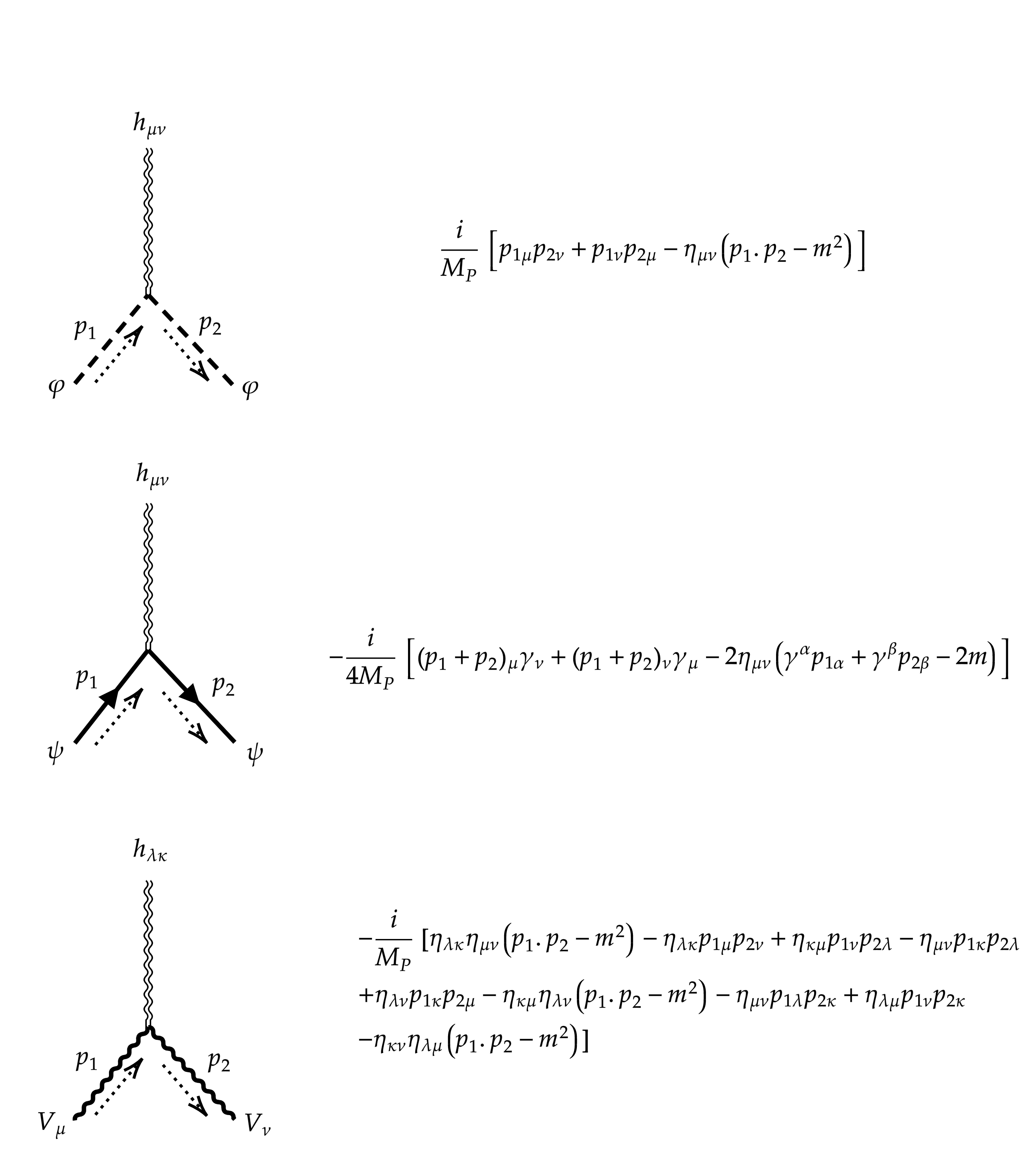
Figure 4: Relevant graviton-matter vertices for scalar $(\varphi)$, fermion $(\psi)$ and vector boson $(V)$, from top to bottom, following Ref. [30].

Appendix B Calculation of the Decay Widths

In this section, we present details of the computation of the differential rates for the inflaton decay into three-body final states, including a graviton.

B.1 Scalar Case

To calculate the differential decay rate and cross-check the results, we present two different strategies based on: $i)$ an explicit construction for the graviton polarization tensor and $ii)$ polarization sum for the massless graviton.

B.1.1 Polarization Tensor in Explicit Form

Without losing generality, we choose a coordinate system in which the graviton moves along the $x$ direction, and hence the four-momentum of the graviton is $\omega=(E_{\omega},\omega_{x},0,0)$, where $\omega^{2}=0$, and then $\omega_{x}=E_{\omega}$. The four-momentum of the inflaton and its other two decay products are $l=(M,0,0,0)$, $p=(E_{p},p_{x},p_{y},p_{z})$, and $q=(M-E_{p}-E_{\omega},-p_{x}-\omega_{x},-p_{y},-p_{z})$, respectively.

The two polarization tensors that meet traceless, transverse, symmetric and orthonormal conditions described in Eqs. (A.1) to (A.4) can be explicitly written as [81]

$$\epsilon^{1}_{\mu\nu}=\frac{1}{\sqrt{2}}\begin{bmatrix}0&0&0&0\\ 0&0&0&0\\ 0&0&1&0\\ 0&0&0&-1\end{bmatrix}\qquad\text{and}\qquad\epsilon^{2}_{\mu\nu}=\frac{1}{\sqrt{2}}\begin{bmatrix}0&0&0&0\\ 0&0&0&0\\ 0&0&0&1\\ 0&0&1&0\end{bmatrix}.$$ (B.1)

Using the Feynman rules of Fig. 4, the amplitudes for the 3-body decays shown in Fig. 1 are

$$i\mathcal{M}_{1} =\frac{-i\,\mu}{M_{P}}\,\frac{l_{\mu}\,l_{\nu}\,\epsilon_{i}^{\star\mu\nu}}{M\,E_{\omega}}=0\,,$$ (B.2)

$$i\mathcal{M}_{2} =\frac{i\,\mu}{M_{P}}\,\frac{p_{\mu}\,p_{\nu}\,\epsilon_{j}^{\star\mu\nu}}{p\cdot\omega}\,,$$ (B.3)

$$i\mathcal{M}_{3} =\frac{i\,\mu}{M_{P}}\,\frac{q_{\mu}\,q_{\nu}\,\epsilon_{k}^{\star\mu\nu}}{M\,E_{\omega}-p\,\cdot\omega}\,,$$ (B.4)

$$i\mathcal{M}_{4} \propto\eta_{\mu\nu}\epsilon^{\mu\nu}=0\,,$$ (B.5)

where $\mathcal{M}_{1,2}$ corresponds to the diagrams in the upper left and upper right panels of Fig. 1, while $\mathcal{M}_{3,4}$ correspond to the lower left and lower right panels, respectively. Using Eq. (B.1), we notice that $\mathcal{M}_{1}=0$ as the decay takes place in the rest frame of the inflaton with $l=(M,0,0,0)$, while

$$\sum_{\text{pol}}|\mathcal{M}_{2}|^{2}=\frac{\mu^{2}}{(p\cdot\omega)^{2}M_{P}^{2}}\sum_{j}(p_{\mu}p_{\nu}\epsilon_{j}^{\star\mu\nu})(p_{\mu}p_{\nu}\epsilon_{j}^{\mu\nu})=\frac{\mu^{2}}{2(p\cdot\omega)^{2}M_{P}^{2}}\left[(p_{y}^{2}-p_{z}^{2})^{2}+4p^{2}_{y}p^{2}_{z}\right].$$ (B.6)

Similarly,

$$\sum_{\text{pol}}|\mathcal{M}_{3}|^{2} =\frac{\mu^{2}}{2(M\,E_{\omega}-p\cdot\omega)^{2}\,M_{P}^{2}}\left[((-p_{y})^{2}-(-p_{z})^{2})^{2}+4p_{y}^{2}p_{z}^{2}\right]$$

$$=\frac{\mu^{2}}{2(M\,E_{\omega}-p\cdot\omega)^{2}\,M_{P}^{2}}\left[(p_{y}^{2}-p_{z}^{2})^{2}+4p_{y}^{2}p_{z}^{2}\right],$$ (B.7)

and the cross-term turns out to be

$$\sum_{\text{pol}}\left(\mathcal{M}_{2}\mathcal{M}^{\star}_{3}\right)=\frac{\mu^{2}}{2(M\,E_{\omega}-p\cdot\omega)(p\cdot\omega)M_{P}^{2}}\left[\left(p_{y}^{2}-p_{z}^{2}\right)^{2}+4\,p_{y}^{2}\,p_{z}^{2}\right].$$ (B.8)

Note that $\sum_{\text{pol}}\left(\mathcal{M}_{1}\mathcal{M}^{\star}_{2}\right)=0$ and $\sum_{\text{pol}}\left(\mathcal{M}_{1}\mathcal{M}^{\star}_{3}\right)=0$ as $\mathcal{M}_{1}=0$. The total squared amplitude is then

$$\sum_{\text{pol}}|\mathcal{M}|^{2}=\frac{\mu^{2}}{2M_{P}^{2}}\left[\frac{1}{p\cdot\omega}+\frac{1}{M\,E_{\omega}-p\cdot\omega}\right]^{2}\left(p_{y}^{2}+p_{z}^{2}\right)^{2}.$$ (B.9)

Since $p\cdot\omega=E_{p}E_{\omega}-p_{x}E_{\omega}$, we have

$$p_{x}=\frac{E_{p}E_{\omega}-p\cdot\omega}{E_{\omega}}\,,$$ (B.10)

which together with $m^{2}\equiv p^{2}=E_{p}^{2}-(p_{x}^{2}+p_{y}^{2}+p_{z}^{2})$ implies

$$\sum_{\text{pol}}|\mathcal{M}|^{2}=\frac{\mu^{2}}{2M_{P}^{2}}\left[\frac{1}{p\cdot\omega}+\frac{1}{M\,E_{\omega}-p\cdot\omega}\right]^{2}\left[2\,\frac{E_{p}}{E_{\omega}}\,p\cdot\omega-\left(\frac{p\cdot\omega}{E_{\omega}}\right)^{2}-m^{2}\right]^{2}$$

$$=\frac{\mu^{2}\left[4E_{\omega}^{2}m^{2}-8E_{p}E_{\omega}M(E_{\omega}+E_{p})+4M^{2}(E_{p}^{2}+3E_{p}E_{\omega}+E_{\omega}^{2})-4(E_{\omega}+E_{p})M^{3}+M^{4})\right]^{2}}{2\,M_{P}^{2}\,E_{\omega}^{2}\,M^{2}\,(M-2\,E_{p})^{2}\left[M-2\,(E_{p}-E_{\omega})\right]^{2}}.$$ (B.11)

Finally, utilizing

$$\frac{d\Gamma}{dE_{\omega}}=\frac{1}{(2\pi)^{3}}\,\frac{1}{8\,M}\int_{E_{p,\text{min}}}^{E_{p,\text{max}}}dE_{p}\,|\mathcal{M}|^{2},$$ (B.12)

with

$$E_{p,\text{max}} =\frac{1}{2}\left[M-E_{\omega}+E_{\omega}\sqrt{\frac{M^{2}-2ME_{\omega}-4m^{2}}{M(M-2E_{\omega})}}\right],$$ (B.13)

$$E_{p,\text{min}} =\frac{1}{2}\left[M-E_{\omega}-E_{\omega}\sqrt{\frac{M^{2}-2ME_{\omega}-4m^{2}}{M(M-2E_{\omega})}}\right],$$ (B.14)

one has the total differential cross-section as

$$\frac{d\Gamma_{0}^{(1)}}{dE_{\omega}}=\frac{2}{64\,\pi^{3}}\left(\frac{\mu}{M_{P}}\right)^{2}\left[\frac{(2x-1)\,(2x-2y^{2}-1)}{4x\,\alpha^{-1}}+\frac{y^{2}(y^{2}+2x-1)}{x}\log\left(\frac{1+\alpha}{1-\alpha}\right)\right]$$ (B.15)

for inflaton decays to complex scalars. Note that the extra factor 2 comes from two possible decay channels of the inflaton.

B.1.2 Polarization Sum

We now employ the second formalism of the calculation, namely the tensor polarization sum formalism, as mentioned in Eq. (A.5). The squared amplitudes are

$$\sum_{\text{pol}}|\mathcal{M}_{1}|^{2} =\frac{\mu^{2}}{M^{2}E_{\omega}^{2}\,M_{P}^{2}}l_{\mu}l_{\nu}l_{\alpha}l_{\beta}\sum_{\text{pol}}\epsilon^{\star\mu\nu}\epsilon^{\alpha\beta}$$

$$=\frac{\mu^{2}}{2M^{2}E_{\omega}^{2}\,M_{P}^{2}}l_{\mu}l_{\nu}l_{\alpha}l_{\beta}\left(\hat{\eta}^{\mu\alpha}\hat{\eta}^{\nu\beta}+\hat{\eta}^{\mu\beta}\hat{\eta}^{\nu\alpha}-\hat{\eta}^{\mu\nu}\hat{\eta}^{\alpha\beta}\right)$$

$$=\frac{\mu^{2}}{2M^{2}E_{\omega}^{2}\,M_{P}^{2}}\left[l^{2}l^{2}-4l^{2}\frac{(l\cdot\omega)(l\cdot\bar{\omega})}{2E_{\omega}^{2}}+4\frac{(l\cdot\omega)^{2}(l\cdot\bar{\omega})^{2}}{4E_{\omega}^{4}}\right]$$

$$=\frac{\mu^{2}}{2\,M^{2}E_{\omega}^{2}\,M_{P}^{2}}\left[l^{2}-\frac{(l\cdot\omega)(l\cdot\bar{\omega})}{E_{\omega}^{2}}\right]^{2}=\frac{\mu^{2}}{2M^{2}E_{\omega}^{2}\,M_{P}^{2}}\left(M^{2}-M^{2}\right)=0\,,$$ (B.16)

$$\sum_{\text{pol}}|\mathcal{M}_{2}|^{2} =\frac{\mu^{2}}{M_{P}^{2}}\,\frac{p_{\mu}\,p_{\nu}\,p_{\alpha}\,p_{\beta}\,}{(p\cdot\omega)^{2}}\,\sum_{\text{pol}}\epsilon^{\star\mu\nu}\epsilon^{\alpha\beta}=\frac{\mu^{2}}{2(p\cdot\omega)^{2}\,M_{P}^{2}}\left[p^{2}-\frac{(p\cdot\omega)(p\cdot\bar{\omega})}{E_{\omega}^{2}}\right]^{2}$$

$$=\frac{\mu^{2}}{2(p\cdot\omega)^{2}\,M_{P}^{2}}\left[m^{2}-\frac{(p\cdot\omega)(p\cdot\bar{\omega})}{E_{\omega}^{2}}\right]^{2},$$ (B.17)

$$\sum_{\text{pol}}|\mathcal{M}_{3}|^{2} =\frac{\mu^{2}}{2(M\,E_{\omega}-p\cdot\omega)^{2}\,M_{P}^{2}}\left[q^{2}-\frac{(q\cdot\omega)(q\cdot\bar{\omega})}{E_{\omega}^{2}}\right]^{2}$$

$$=\frac{\mu^{2}}{2(M\,E_{\omega}-p\cdot\omega)^{2}\,M_{P}^{2}}\left[m^{2}-\frac{(q\cdot\omega)(q\cdot\bar{\omega})}{E_{\omega}^{2}}\right]^{2},$$ (B.18)

$$\sum_{\text{pol}}\left(\mathcal{M}_{2}\mathcal{M}^{\star}_{3}\right) =\frac{\mu^{2}}{(p\cdot\omega)(M\,E_{\omega}-p\cdot\omega)\,M_{P}^{2}}p_{\mu}p_{\nu}q_{\alpha}q_{\beta}\sum_{\text{pol}}\epsilon^{\star\mu\nu}\epsilon^{\alpha\beta}$$

$$=\frac{\mu^{2}}{2(p\cdot\omega)(M\,E_{\omega}-p\cdot\omega)M_{P}^{2}}\,\Bigg{\{}2\left[(p\cdot q)-\frac{(p\cdot\omega)(q\cdot\bar{\omega})+(p\cdot\bar{\omega})(q\cdot\omega)}{2E_{\omega}^{2}}\right]^{2}$$

$$\qquad-\left[p^{2}q^{2}-\frac{p^{2}(q\cdot\omega)(q\cdot\bar{\omega})+q^{2}(p\cdot\omega)(p\cdot\bar{\omega})}{E_{\omega}^{2}}+\frac{(p\cdot\omega)(p\cdot\bar{\omega})(q\cdot\omega)(q\cdot\bar{\omega})}{E_{\omega}^{4}}\right]\Bigg{\}}$$

$$=\frac{\mu^{2}}{2(p\cdot\omega)(M\,E_{\omega}-p\cdot\omega)M_{P}^{2}}\,\Bigg{\{}2\left[(p\cdot q)-\frac{(p\cdot\omega)(q\cdot\bar{\omega})+(p\cdot\bar{\omega})(q\cdot\omega)}{2E_{\omega}^{2}}\right]^{2}$$

$$\qquad-\left[p^{2}-\frac{(q\cdot\omega)(q\cdot\bar{\omega})}{E_{\omega}^{2}}\right]\left[q^{2}-\frac{(p\cdot\omega)(p\cdot\bar{\omega})}{E_{\omega}^{2}}\right]\Bigg{\}}.$$ (B.19)

Note that Eq. (B.1.2) implies $\mathcal{M}_{1}=0$, which agrees with Eq. (B.2). Therefore, the other two interference terms $\sum_{\text{pol}}\left(\mathcal{M}_{1}\mathcal{M}^{\star}_{2}\right)=\sum_{\text{pol}}\left(\mathcal{M}_{1}\mathcal{M}^{\star}_{3}\right)=0$. Using the four vectors, one ends up with

$$p\cdot\omega =M\left(E_{\omega}+E_{p}-\frac{1}{2}M\right),$$ (B.20)

$$p\cdot\bar{\omega} =2E_{p}E_{\omega}-p\cdot\omega\,,$$ (B.21)

$$q\cdot\omega =ME_{\omega}-p\cdot\omega\,,$$ (B.22)

$$q\cdot\bar{\omega} =(l-p-\omega)\bar{\omega}=ME_{\omega}-p\cdot\bar{\omega}-2E_{\omega}^{2}=ME_{\omega}-2E_{p}E_{\omega}+p\cdot\omega-2E_{\omega}^{2}\,,$$ (B.23)

$$p\cdot q =\frac{1}{2}\left[(p+q)^{2}-2m^{2}\right]=\frac{1}{2}\left[(l-\omega)^{2}-2m^{2}\right]=\frac{1}{2}\left[M^{2}-2ME_{\omega}-2m^{2}\right].$$ (B.24)

With these relations, one obtains

$$\sum_{\text{pol}}|\mathcal{M}|^{2} =\frac{\mu^{2}\left[4E_{\omega}^{2}m^{2}-8E_{p}E_{\omega}M(E_{\omega}+E_{p})+4M^{2}(E_{p}^{2}+3E_{p}E_{\omega}+E_{\omega}^{2})-4(E_{\omega}+E_{p})M^{3}+M^{4})\right]^{2}}{2M_{P}^{2}E_{\omega}^{2}M^{2}(M-2E_{p})^{2}[M-2(E_{p}-E_{\omega})]^{2}},$$ (B.25)

and further

$$\frac{d\Gamma_{0}^{(1)}}{dE_{\omega}}=\frac{\mu^{2}}{32\pi^{3}M_{P}^{2}}\left[\frac{(2x-1)\,(2x-2y^{2}-1)}{4x\,\alpha^{-1}}+\frac{y^{2}(y^{2}+2x-1)}{x}\log\left(\frac{1+\alpha}{1-\alpha}\right)\right],$$ (B.26)

which agrees with Eq. (B.15).

B.2 Fermionic Case

Using the list of Feynman rules in Fig. 4, the amplitudes for the inflaton decay into a Dirac fermion turn out to be

$$i\mathcal{M}_{1} =-i\,\frac{y_{\psi}}{M_{P}}\,\frac{l_{\mu}\,l_{\nu}\,\epsilon^{\star\mu\nu}}{M\,E_{\omega}}\bar{u}(p)v(q)\,,$$ (B.27)

$$i\mathcal{M}_{2} =\frac{iy_{\psi}}{2p\cdot\omega M_{P}}\left[\bar{u}(p)(p_{\mu}\gamma_{\nu})(\not{l}+2m)v(q)\right]\epsilon^{*\mu\nu},$$ (B.28)

$$i\mathcal{M}_{3} =\frac{iy_{\psi}}{2(ME_{\omega}-p\cdot\omega)M_{P}}\left[\bar{u}(p)(\not{l}-2m))(q_{\mu}\gamma_{\nu})v(q)\right]\epsilon^{*\mu\nu},$$ (B.29)

$$i\mathcal{M}_{4} \propto\eta_{\mu\nu}\epsilon^{*\mu\nu}=0\,,$$ (B.30)

where $\mathcal{M}_{1},\mathcal{M}_{2},\mathcal{M}_{3}~{}\text{and}~{}\mathcal{M}_{4}$ corresponds to the diagrams from left to right in Fig. 5. Note that

$$\sum_{\text{spin, pol}}|\mathcal{M}_{1}|^{2} =\frac{y_{\psi}^{2}}{M^{2}E_{\omega}^{2}\,M_{P}^{2}}l_{\mu}l_{\nu}l_{\alpha}l_{\beta}\sum_{\text{pol}}\epsilon^{\star\mu\nu}\epsilon^{\alpha\beta}\times\text{Tr}\left[(\not{q}-m)(\not{p}+m)\right]\,$$

$$=\eqref{eq:M1square_scalar}\times\frac{y_{\psi}^{2}}{\mu^{2}}\times\text{Tr}\left[(\not{q}-m)(\not{p}+m)\right]=0\,,$$ (B.31)

which again implies that $\mathcal{M}_{1}=0$. In fact, since $\mathcal{M}_{1}\propto$ Eq. (B.2), one immediately finds that it vanishes.

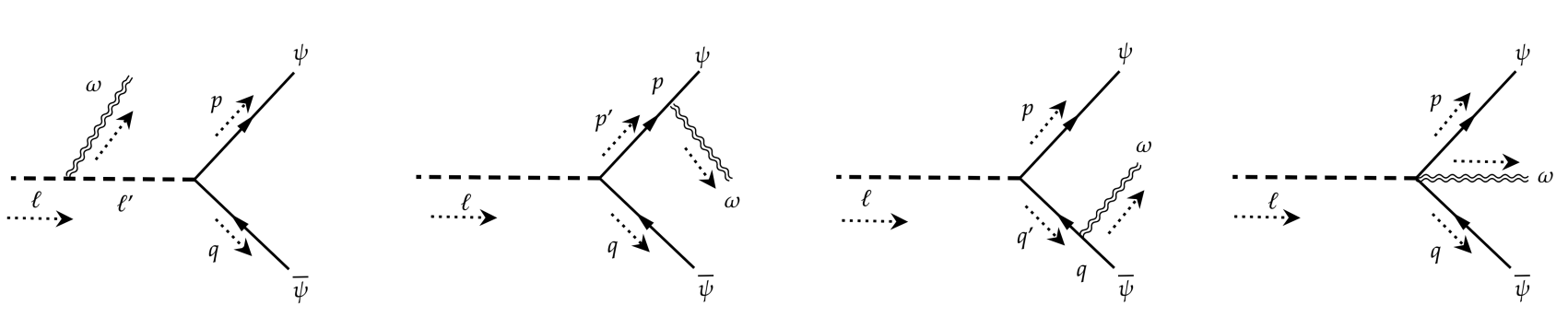
Figure 5: Feynman graph for inflaton decay into a pair of Dirac fermions with graviton emission.

The other squared amplitudes are given by:

$$\sum_{\text{spin, pol}}|\mathcal{M}_{2}|^{2} =\frac{y_{\psi}^{2}}{(2p\cdot\omega)^{2}\,M_{P}^{2}}\sum_{\text{pol}}\epsilon^{\star\mu\nu}\epsilon^{\alpha\beta}$$

$$\times\text{Tr}\left[p_{\mu}\gamma_{\nu}(\not{l}+2m)(\not{q}-m)(\not{l}+2m)\gamma_{\alpha}p_{\beta}(\not{p}+m)\right],$$ (B.32)

$$\sum_{\text{spin, pol}}|\mathcal{M}_{3}|^{2} =\frac{y_{\psi}^{2}}{4(ME_{\omega}-p\cdot\omega)^{2}\,M_{P}^{2}}\sum_{\text{pol}}\epsilon^{\star\mu\nu}\epsilon^{\alpha\beta}$$

$$\times\text{Tr}\left[(\not{l}-2m)q_{\mu}\gamma_{\nu}(\not{q}-m)\gamma_{\alpha}q_{\beta}(\not{l}-2m)(\not{p}+m)\right],$$ (B.33)

$$\sum_{\text{spin, pol}}(\mathcal{M}_{2}\mathcal{M}_{3}^{*}) =\frac{y_{\psi}^{2}}{4p\cdot\omega(ME_{\omega}-p\cdot\omega)\,M_{P}^{2}}\sum_{\text{pol}}\epsilon^{\star\mu\nu}\epsilon^{\alpha\beta}$$

$$\times\text{Tr}\left[p_{\mu}\gamma_{\nu}(\not{l}+2m)(\not{q}-m)\gamma_{\alpha}q_{\beta}(\not{l}-2m)(\not{p}+m)\right].$$ (B.34)

Similarly as before, the other interference terms $\sum_{\text{pol}}\left(\mathcal{M}_{1}\mathcal{M}^{\star}_{2}\right)=\sum_{\text{pol}}\left(\mathcal{M}_{1}\mathcal{M}^{\star}_{3}\right)=0$. The total matrix element squared turns out to be

$$\sum_{\text{spin, pol}}|\mathcal{M}|^{2}=y_{\psi}^{2}\frac{M(M-2E_{p})(M-2E_{\omega})(2(E_{p}+E_{\omega})-M)+4E_{\omega}^{2}m^{2}}{E_{\omega}^{2}M^{2}(M-2E_{p}^{2})(M-2(E_{p}+E_{\omega}))^{2}M_{P}^{2}}$$

$$\qquad\quad\times\Big{\{}4Mm^{2}\left[M(4E_{p}^{2}+12E_{p}E_{\omega}+3E_{\omega}^{2})-4M^{2}(E_{p}+E_{\omega})-8E_{p}E_{\omega}(E_{p}+E_{\omega})+M^{3}\right]$$

$$\qquad\quad-M^{2}(M-2E_{p})(2E_{\omega}^{2}-2E_{\omega}M+M^{2})\left[M-2(E_{p}+E_{\omega})\right]+16E_{\omega}^{2}m^{4}\Big{\}},$$ (B.35)

with which we find

$$\frac{d\Gamma_{1/2}^{(1)}}{dE_{\omega}}=\frac{y_{\psi}^{2}M^{2}}{64\,\pi^{3}\,M_{P}^{2}} \Bigg{[}\frac{(1-2x)}{x\alpha^{-1}}\left[8xy^{2}+2(x-1)x-8y^{4}-2y^{2}+1\right]$$

$$+\frac{4y^{2}\left[(5-8x)y^{2}-(x-1)^{2}-4y^{4}\right]}{x}\log\left(\frac{1+\alpha}{1-\alpha}\right)\Bigg{]}.$$ (B.36)

B.3 Vector Case

For the amplitudes of inflaton decay into massive spin-1 final states, we obtain

$$i\mathcal{M}_{1}=-i\,\frac{2\,g_{V}}{M_{P}}\,\frac{l_{\mu}\,l_{\nu}\,\epsilon^{\star\mu\nu}}{M\,E_{\omega}}\eta_{\mu^{\prime}\nu^{\prime}}\varepsilon^{*\mu^{\prime}}(p,\lambda)\varepsilon^{*\nu^{\prime}}(q,\lambda)\,,$$ (B.37)

and similarly, we find

$$i\mathcal{M}_{2} =-i\frac{g_{V}}{p\cdot\omega\,M_{P}}\,\epsilon^{*\mu\nu}\varepsilon^{*\mu^{\prime}}(p,\lambda)\varepsilon^{*\nu^{\prime}}(q,\lambda)\cdot\eta_{\sigma\nu^{\prime}}\left[\eta^{\rho\sigma}-\frac{(p^{\prime\rho}p^{\prime\sigma})}{m^{2}}\right]$$

$$\quad\times\left[\eta_{\mu\nu}\eta_{\rho\mu^{\prime}}\left(p^{\prime}\cdot p-m^{2}\right)-\eta_{\mu\nu}p^{\prime}_{\mu^{\prime}}p_{\rho}\right.+\eta_{\nu\rho}p^{\prime}_{\mu^{\prime}}p_{\mu}-\eta_{\rho\mu^{\prime}}p^{\prime}_{\nu}p_{\mu}+\eta_{\mu\mu^{\prime}}p^{\prime}_{\nu}p_{\rho}$$

$$\quad-\eta_{\nu\rho}\eta_{\mu\mu^{\prime}}\left(p^{\prime}\cdot p-m^{2}\right)+\eta_{\nu\mu^{\prime}}p^{\prime}_{\mu}p_{\rho}-\eta_{\rho\mu^{\prime}}p^{\prime}_{\mu}p_{\nu}+\eta_{\mu\rho}p^{\prime}_{\mu^{\prime}}p_{\nu}\left.-\eta_{\nu\mu^{\prime}}\eta_{\mu\rho}\left(p^{\prime}\cdot p-m^{2}\right)\right],$$ (B.38)

$$i\mathcal{M}_{3} =-i\frac{g_{V}}{(ME_{\omega}-p\cdot\omega)\,M_{P}}\,\epsilon^{*\mu\nu}\varepsilon^{*\mu^{\prime}}(p,\lambda)\varepsilon^{*\nu^{\prime}}(q,\lambda)\cdot\eta_{\sigma\mu^{\prime}}\left[\eta^{\rho\sigma}-\frac{(q^{\prime\rho}q^{\prime\sigma})}{m^{2}}\right]$$

$$\quad\times\left[\eta_{\mu\nu}\eta_{\rho\nu^{\prime}}\left(q^{\prime}\cdot q-m^{2}\right)-\eta_{\mu\nu}q^{\prime}_{\nu^{\prime}}q_{\rho}\right.+\eta_{\nu\rho}q^{\prime}_{\nu^{\prime}}q_{\mu}-\eta_{\rho\nu^{\prime}}q^{\prime}_{\nu}q_{\mu}+\eta_{\mu\nu^{\prime}}q^{\prime}_{\nu}q_{\rho}$$

$$\quad-\eta_{\nu\rho}\eta_{\mu\nu^{\prime}}\left(q^{\prime}\cdot q-m^{2}\right)+\eta_{\nu\nu^{\prime}}q^{\prime}_{\mu}q_{\rho}-\eta_{\rho\nu^{\prime}}q^{\prime}_{\mu}q_{\nu}+\eta_{\mu\rho}q^{\prime}_{\nu^{\prime}}q_{\nu}\left.-\eta_{\nu\nu^{\prime}}\eta_{\mu\rho}\left(q^{\prime}\cdot q-m^{2}\right)\right],$$ (B.39)

while

$$\mathcal{M}_{4}\propto\eta_{\mu\nu}\epsilon^{*\mu\nu}=0\,,$$ (B.40)

for left to right in Fig. 6, respectively.

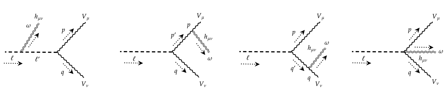
Figure 6: Feynman diagrams for inflaton decay into a pair of massive vectors with graviton emission.

The total squared matrix element is given by

$$\sum_{\text{spin, pol}}|\mathcal{M}|^{2}=\frac{g_{V}^{2}}{2E_{\omega}^{4}\,M^{2}\,m^{4}(M-2E_{p})^{2}(M-2E_{p}-2E_{\omega})^{2}M_{P}^{2}}\times\sum_{k=0}^{8}\,\mathcal{A}_{k}\,E_{p}^{k}\,,$$ (B.41)

where

$$\mathcal{A}_{8} =256M^{4}(M-2E_{\omega})^{2},$$ (B.42)

$$\mathcal{A}_{7} =1024(E_{\omega}-M)M^{4}(M-2E_{\omega})^{2},$$ (B.43)

$$\mathcal{A}_{6} =128(2E_{\omega}-M)M^{3}\Big{[}-2E_{\omega}(M-4E_{\omega})m^{2}-M(M-2E_{\omega})(12E_{\omega}^{2}-27ME_{\omega}+14M^{2})\Big{]},$$ (B.44)

$$\mathcal{A}_{5} =128M^{3}(2E_{\omega}^{2}-3ME_{\omega}+M^{2})$$

$$\qquad\times\Big{[}-6E_{\omega}(M-4E_{\omega})m^{2}-M(M-2E_{\omega})(8E_{\omega}^{2}-25ME_{\omega}+14M^{2})\Big{]},$$ (B.45)

$$\mathcal{A}_{4} =16M^{3}\Big{[}4E_{\omega}^{2}(3M-4E_{\omega})m^{4}$$

$$\qquad+4E_{\omega}(M-2E_{\omega})(-60E_{\omega}^{3}+138ME_{\omega}^{2}-91M^{2}E_{\omega}+15M^{3})\,m^{2}$$

$$\qquad+M(M-2E_{\omega})^{2}(16E_{\omega}^{4}-136ME_{\omega}^{3}+301M^{2}E_{\omega}^{2}-250M^{3}E_{\omega}+70M^{4})\Big{]},$$ (B.46)

$$\mathcal{A}_{3} =-32(E_{\omega}-M)M^{3}\Big{[}4E_{\omega}^{2}(4E_{\omega}-3M)m^{4}-4E_{\omega}(2E_{\omega}-M)$$

$$\qquad\times(20E_{\omega}^{3}-48ME_{\omega}^{2}+31M^{2}E_{\omega}-5M^{3})m^{2}+M^{2}\,(M-2E_{\omega})^{2}$$

$$\qquad\times(12E_{\omega}^{3}-45ME_{\omega}^{2}+46M^{2}E_{\omega}-14M^{3})\Big{]},$$ (B.47)

$$\mathcal{A}_{2} =8M\Big{[}M^{5}(M-2E_{\omega})(M-E_{\omega})(-26E_{\omega}^{3}+68ME_{\omega}^{2}-55M^{2}E_{\omega}+14M^{3})$$

$$+2E_{\omega}M^{2}(M-2E_{\omega})(-56E_{\omega}^{5}+264ME_{\omega}^{4}-458M^{2}E_{\omega}^{3}+360M^{3}E_{\omega}^{2}-126M^{4}E_{\omega}+15M^{5})m^{2}$$

$$+16E_{\omega}^{4}(3M-4E_{\omega})m^{6}+4E_{\omega}^{2}M(-24E_{\omega}^{4}+4ME_{\omega}^{3}+26M^{2}E_{\omega}^{2}-30M^{3}E_{\omega}+9M^{4})m^{4}\Big{]},$$ (B.48)

$$\mathcal{A}_{1} =8(E_{\omega}-M)M\Big{[}(2M-3E_{\omega})(E_{\omega}-M)(2E_{\omega}-M)^{3}M^{6}$$

$$\quad+2E_{\omega}(2E_{\omega}-3M)(M-2E_{\omega})^{2}(2E_{\omega}^{3}-8ME_{\omega}^{2}+6M^{2}E_{\omega}-M^{3})m^{2}M^{2}$$

$$\quad+4E_{\omega}^{2}(-24E_{\omega}^{4}+12ME_{\omega}^{3}+4M^{2}E_{\omega}^{2}-10M^{3}E_{\omega}+3M^{4})m^{4}M+16E_{\omega}^{4}(3M-4E_{\omega})m^{6}\Big{]},$$ (B.49)

$$\mathcal{A}_{0} =192\,E_{\omega}^{6}\,m^{8}+32\,E_{\omega}^{4}\,M^{2}(6\,E_{\omega}^{2}-10\,M\,E_{\omega}+3\,M^{2})\,m^{6}+(E_{\omega}-M)^{2}\,M^{8}\,(M-2E_{\omega})^{4}$$

$$-4\,E_{\omega}^{2}\,M^{2}\,(2\,E_{\omega}^{2}-2\,M\,E_{\omega}+M^{2})(16\,E_{\omega}^{4}-32\,M\,E_{\omega}^{3}+6\,M^{2}\,E_{\omega}^{2}+10\,M^{3}\,E_{\omega}-3\,M^{4})\,m^{4}$$

$$-4\,E_{\omega}\,M^{4}\,(M-2E_{\omega})^{4}\,(2\,E_{\omega}^{3}-4\,ME_{\omega}^{2}+5\,M^{2}\,E_{\omega}-M^{3})\,m^{2},$$ (B.50)

with which one can show that the differential decay rate reads

$$\frac{d\Gamma^{(1)}_{1}}{dE_{\omega}} =\frac{g_{V}^{2}}{1920\,\pi^{3}\,x\,y^{4}\,M_{P}^{2}}$$

$$\Bigg{[}60y^{2}\left(-(1-2x)^{2}(1+2x)+(5+4x(-3+4x))y^{2}+16(x-1)y^{4}+12y^{6}\right)\log\left(\frac{1+\alpha}{1-\alpha}\right)$$

$$+\alpha\Big{(}360(1-2x)y^{6}+4(4x(23x-5)+15)y^{4}+2(2x-1)(28x(14x-5)+15)y^{2}$$

$$+(1-2x)^{2}(4x(2x-5)+15)\Big{)}\Bigg{]}.$$ (B.51)

References

- [1] A.A. Starobinsky, Spectrum of relict gravitational radiation and the early state of the universe, JETP Lett. 30 (1979) 682.
- [2] B. Allen, The Stochastic Gravity Wave Background in Inflationary Universe Models, Phys. Rev. D 37 (1988) 2078.
- [3] V. Sahni, The Energy Density of Relic Gravity Waves From Inflation, Phys. Rev. D 42 (1990) 453.
- [4] M.S. Turner, M.J. White and J.E. Lidsey, Tensor perturbations in inflationary models as a probe of cosmology, Phys. Rev. D 48 (1993) 4613 [astro-ph/9306029].
- [5] S.Y. Khlebnikov and I.I. Tkachev, Relic gravitational waves produced after preheating, Phys. Rev. D 56 (1997) 653 [hep-ph/9701423].
- [6] R. Easther and E.A. Lim, Stochastic gravitational wave production after inflation, JCAP 04 (2006) 010 [astro-ph/0601617].
- [7] J.F. Dufaux, A. Bergman, G.N. Felder, L. Kofman and J.-P. Uzan, Theory and Numerics of Gravitational Waves from Preheating after Inflation, Phys. Rev. D 76 (2007) 123517 [0707.0875].
- [8] L. Bethke, D.G. Figueroa and A. Rajantie, Anisotropies in the Gravitational Wave Background from Preheating, Phys. Rev. Lett. 111 (2013) 011301 [1304.2657].
- [9] D.G. Figueroa and F. Torrenti, Gravitational wave production from preheating: parameter dependence, JCAP 10 (2017) 057 [1707.04533].
- [10] A. Vilenkin, Gravitational radiation from cosmic strings, Phys. Lett. B 107 (1981) 47.
- [11] Y. Cui, M. Lewicki, D.E. Morrissey and J.D. Wells, Cosmic Archaeology with Gravitational Waves from Cosmic Strings, Phys. Rev. D 97 (2018) 123505 [1711.03104].
- [12] Y. Cui, M. Lewicki, D.E. Morrissey and J.D. Wells, Probing the pre-BBN universe with gravitational waves from cosmic strings, JHEP 01 (2019) 081 [1808.08968].
- [13] C.-F. Chang and Y. Cui, Gravitational waves from global cosmic strings and cosmic archaeology, JHEP 03 (2022) 114 [2106.09746].
- [14] J. Ghiglieri and M. Laine, Gravitational wave background from Standard Model physics: Qualitative features, JCAP 07 (2015) 022 [1504.02569].
- [15] J. Ghiglieri, G. Jackson, M. Laine and Y. Zhu, Gravitational wave background from Standard Model physics: Complete leading order, JHEP 07 (2020) 092 [2004.11392].
- [16] J. Ghiglieri, J. Schütte-Engel and E. Speranza, Freezing-In Gravitational Waves, 2211.16513.
- [17] K. Nakayama and Y. Tang, Stochastic Gravitational Waves from Particle Origin, Phys. Lett. B 788 (2019) 341 [1810.04975].
- [18] D. Huang and L. Yin, Stochastic Gravitational Waves from Inflaton Decays, Phys. Rev. D 100 (2019) 043538 [1905.08510].
- [19] Y. Mambrini, K.A. Olive and J. Zheng, Post-inflationary dark matter bremsstrahlung, JCAP 10 (2022) 055 [2208.05859].
- [20] S. Weinberg, Infrared photons and gravitons, Phys. Rev. 140 (1965) B516.
- [21] J.F. Dufaux, G.N. Felder, L. Kofman, M. Peloso and D. Podolsky, Preheating with trilinear interactions: Tachyonic resonance, JCAP 07 (2006) 006 [hep-ph/0602144].
- [22] A. Ghoshal, R. Samanta and G. White, Bremsstrahlung High-frequency Gravitational Wave Signatures of High-scale Non-thermal Leptogenesis, 2211.10433.
- [23] L. Pagano, L. Salvati and A. Melchiorri, New constraints on primordial gravitational waves from Planck 2015, Phys. Lett. B 760 (2016) 823 [1508.02393].
- [24] C. Caprini and D.G. Figueroa, Cosmological Backgrounds of Gravitational Waves, Class. Quant. Grav. 35 (2018) 163001 [1801.04268].
- [25] A. Berlin, D. Blas, R. Tito D’Agnolo, S.A.R. Ellis, R. Harnik, Y. Kahn et al., Detecting high-frequency gravitational waves with microwave cavities, Phys. Rev. D 105 (2022) 116011 [2112.11465].
- [26] N. Herman, L. Lehoucq and A. Fúzfa, Electromagnetic Antennas for the Resonant Detection of the Stochastic Gravitational Wave Background, 2203.15668.
- [27] N. Seto, S. Kawamura and T. Nakamura, Possibility of direct measurement of the acceleration of the universe using 0.1-Hz band laser interferometer gravitational wave antenna in space, Phys. Rev. Lett. 87 (2001) 221103 [astro-ph/0108011].
- [28] H. Kudoh, A. Taruya, T. Hiramatsu and Y. Himemoto, Detecting a gravitational-wave background with next-generation space interferometers, Phys. Rev. D 73 (2006) 064006 [gr-qc/0511145].
- [29] N. Aggarwal et al., Challenges and opportunities of gravitational-wave searches at MHz to GHz frequencies, Living Rev. Rel. 24 (2021) 4 [2011.12414].
- [30] S.Y. Choi, J.S. Shim and H.S. Song, Factorization and polarization in linearized gravity, Phys. Rev. D 51 (1995) 2751 [hep-th/9411092].
- [31] L. Kofman, A.D. Linde and A.A. Starobinsky, Towards the theory of reheating after inflation, Phys. Rev. D 56 (1997) 3258 [hep-ph/9704452].
- [32] M. Drewes, Measuring the inflaton coupling in the CMB, JCAP 09 (2022) 069 [1903.09599].
- [33] M. Drewes and L. Ming, Connecting Cosmic Inflation to Particle Physics with LiteBIRD, CMB S4, EUCLID and SKA, 2208.07609.
- [34] M. Drees and Y. Xu, Small field polynomial inflation: reheating, radiative stability and lower bound, JCAP 09 (2021) 012 [2104.03977].
- [35] M. Peloso and L. Sorbo, Preheating of massive fermions after inflation: Analytical results, JHEP 05 (2000) 016 [hep-ph/0003045].
- [36] G.N. Felder, L. Kofman and A.D. Linde, Instant preheating, Phys. Rev. D 59 (1999) 123523 [hep-ph/9812289].
- [37] P. Klose, M. Laine and S. Procacci, Gravitational wave background from non-Abelian reheating after axion-like inflation, JCAP 05 (2022) 021 [2201.02317].
- [38] S. Sarkar, Big bang nucleosynthesis and physics beyond the standard model, Rept. Prog. Phys. 59 (1996) 1493 [hep-ph/9602260].
- [39] M. Kawasaki, K. Kohri and N. Sugiyama, MeV scale reheating temperature and thermalization of neutrino background, Phys. Rev. D 62 (2000) 023506 [astro-ph/0002127].
- [40] S. Hannestad, What is the lowest possible reheating temperature?, Phys. Rev. D 70 (2004) 043506 [astro-ph/0403291].
- [41] F. De Bernardis, L. Pagano and A. Melchiorri, New constraints on the reheating temperature of the universe after WMAP-5, Astropart. Phys. 30 (2008) 192.
- [42] P.F. de Salas, M. Lattanzi, G. Mangano, G. Miele, S. Pastor and O. Pisanti, Bounds on very low reheating scenarios after Planck, Phys. Rev. D 92 (2015) 123534 [1511.00672].
- [43] S. Dodelson and M.S. Turner, Nonequilibrium neutrino statistical mechanics in the expanding universe, Phys. Rev. D 46 (1992) 3372.
- [44] S. Hannestad and J. Madsen, Neutrino decoupling in the early universe, Phys. Rev. D 52 (1995) 1764 [astro-ph/9506015].
- [45] A.D. Dolgov, S.H. Hansen and D.V. Semikoz, Nonequilibrium corrections to the spectra of massless neutrinos in the early universe, Nucl. Phys. B 503 (1997) 426 [hep-ph/9703315].
- [46] G. Mangano, G. Miele, S. Pastor, T. Pinto, O. Pisanti and P.D. Serpico, Relic neutrino decoupling including flavor oscillations, Nucl. Phys. B 729 (2005) 221 [hep-ph/0506164].
- [47] P.F. de Salas and S. Pastor, Relic neutrino decoupling with flavour oscillations revisited, JCAP 07 (2016) 051 [1606.06986].
- [48] M. Escudero Abenza, Precision early universe thermodynamics made simple: and neutrino decoupling in the Standard Model and beyond, JCAP 05 (2020) 048 [2001.04466].
- [49] K. Akita and M. Yamaguchi, A precision calculation of relic neutrino decoupling, JCAP 08 (2020) 012 [2005.07047].
- [50] J. Froustey, C. Pitrou and M.C. Volpe, Neutrino decoupling including flavour oscillations and primordial nucleosynthesis, JCAP 12 (2020) 015 [2008.01074].
- [51] J.J. Bennett, G. Buldgen, P.F. De Salas, M. Drewes, S. Gariazzo, S. Pastor et al., Towards a precision calculation of in the Standard Model II: Neutrino decoupling in the presence of flavour oscillations and finite-temperature QED, JCAP 04 (2021) 073 [2012.02726].
- [52] M. Drees, F. Hajkarim and E.R. Schmitz, The Effects of QCD Equation of State on the Relic Density of WIMP Dark Matter, JCAP 06 (2015) 025 [1503.03513].
- [53] G.F. Giudice, E.W. Kolb and A. Riotto, Largest temperature of the radiation era and its cosmological implications, Phys. Rev. D 64 (2001) 023508 [hep-ph/0005123].
- [54] Planck collaboration, Planck 2018 results. VI. Cosmological parameters, Astron. Astrophys. 641 (2020) A6 [1807.06209].
- [55] BICEP, Keck collaboration, Improved Constraints on Primordial Gravitational Waves using Planck, WMAP, and BICEP/Keck Observations through the 2018 Observing Season, Phys. Rev. Lett. 127 (2021) 151301 [2110.00483].
- [56] T.-H. Yeh, J. Shelton, K.A. Olive and B.D. Fields, Probing physics beyond the standard model: limits from BBN and the CMB independently and combined, JCAP 10 (2022) 046 [2207.13133].
- [57] K. Abazajian et al., CMB-S4 Science Case, Reference Design, and Project Plan, 1907.04473.
- [58] CMB-HD collaboration, Snowmass2021 CMB-HD White Paper, 2203.05728.
- [59] COrE collaboration, COrE (Cosmic Origins Explorer) A White Paper, 1102.2181.
- [60] EUCLID collaboration, Euclid Definition Study Report, 1110.3193.
- [61] I. Ben-Dayan, B. Keating, D. Leon and I. Wolfson, Constraints on scalar and tensor spectra from , JCAP 06 (2019) 007 [1903.11843].
- [62] SPT-3G collaboration, SPT-3G: A Next-Generation Cosmic Microwave Background Polarization Experiment on the South Pole Telescope, Proc. SPIE Int. Soc. Opt. Eng. 9153 (2014) 91531P [1407.2973].
- [63] Simons Observatory collaboration, The Simons Observatory: Science goals and forecasts, JCAP 02 (2019) 056 [1808.07445].
- [64] A. Ringwald, J. Schütte-Engel and C. Tamarit, Gravitational Waves as a Big Bang Thermometer, JCAP 03 (2021) 054 [2011.04731].
- [65] A. Ringwald and C. Tamarit, Revealing the cosmic history with gravitational waves, Phys. Rev. D 106 (2022) 063027 [2203.00621].
- [66] M. Maggiore, Gravitational wave experiments and early universe cosmology, Phys. Rept. 331 (2000) 283 [gr-qc/9909001].
- [67] LISA collaboration, Laser Interferometer Space Antenna, arXiv e-prints (2017) arXiv:1702.00786 [1702.00786].
- [68] M. Punturo et al., The Einstein Telescope: A third-generation gravitational wave observatory, Class. Quant. Grav. 27 (2010) 194002.
- [69] S. Hild et al., Sensitivity Studies for Third-Generation Gravitational Wave Observatories, Class. Quant. Grav. 28 (2011) 094013 [1012.0908].
- [70] B. Sathyaprakash et al., Scientific Objectives of Einstein Telescope, Class. Quant. Grav. 29 (2012) 124013 [1206.0331].
- [71] M. Maggiore et al., Science Case for the Einstein Telescope, JCAP 03 (2020) 050 [1912.02622].
- [72] J. Crowder and N.J. Cornish, Beyond LISA: Exploring future gravitational wave missions, Phys. Rev. D 72 (2005) 083005 [gr-qc/0506015].
- [73] V. Corbin and N.J. Cornish, Detecting the cosmic gravitational wave background with the big bang observer, Class. Quant. Grav. 23 (2006) 2435 [gr-qc/0512039].
- [74] G.M. Harry, P. Fritschel, D.A. Shaddock, W. Folkner and E.S. Phinney, Laser interferometry for the big bang observer, Class. Quant. Grav. 23 (2006) 4887.
- [75] F.-Y. Li, M.-X. Tang and D.-P. Shi, Electromagnetic response of a Gaussian beam to high frequency relic gravitational waves in quintessential inflationary models, Phys. Rev. D 67 (2003) 104008 [gr-qc/0306092].
- [76] E. Armengaud et al., Conceptual Design of the International Axion Observatory (IAXO), JINST 9 (2014) T05002 [1401.3233].
- [77] IAXO collaboration, Physics potential of the International Axion Observatory (IAXO), JCAP 06 (2019) 047 [1904.09155].
- [78] D.J. Gross and R. Jackiw, Low-Energy Theorem for Graviton Scattering, Phys. Rev. 166 (1968) 1287.
- [79] T. Gleisberg, F. Krauss, K.T. Matchev, A. Schalicke, S. Schumann and G. Soff, Helicity formalism for spin-2 particles, JHEP 09 (2003) 001 [hep-ph/0306182].
- [80] P. de Aquino, K. Hagiwara, Q. Li and F. Maltoni, Simulating graviton production at hadron colliders, JHEP 06 (2011) 132 [1101.5499].
- [81] H. van Dam and M.J.G. Veltman, Massive and massless Yang-Mills and gravitational fields, Nucl. Phys. B 22 (1970) 397.