The Gaia-Kepler-TESS-Host Stellar Properties Catalog: Uniform Physical Parameters for 7993 Host Stars and 9324 Planets

Abstract

We present the first homogeneous catalog of Kepler, K2, and TESS host stars and the corresponding catalog of exoplanet properties, which contain 7993 stars and 9324 planets, respectively. We used isochrone fitting and Gaia DR3 photometry, parallaxes, and spectrophotometric metallicities to compute precise, homogeneous $T_{\mathrm{eff}}$, $\log g$, masses, radii, mean stellar densities, luminosities, ages, distances, and V-band extinctions for 3248, 565, and 4180 Kepler, K2, and TESS stars, respectively. We compared our stellar properties to studies using fundamental and precise constraints, such as interferometry and asteroseismology, and find residual scatters of 2.8%, 5.6%, 5.0%, and 31%, with offsets of 0.2%, 1.0%, 1.2%, and 0.7% between our $T_{\mathrm{eff}}$, radii, masses, and ages and those in the literature, respectively. In addition, we compute planet radii, semimajor axes, and incident fluxes for 4281, 676, and 4367 Kepler, K2, and TESS planets, respectively, and find that the exoplanet radius gap is less prominent in the K2, TESS, and combined samples than it is in the Kepler sample alone. We suspect this difference is largely due to heterogeneous planet-to-star radius ratios, shorter time baselines of K2 and TESS, and smaller sample sizes. Finally, we identify a clear radius inflation trend in our large sample of hot Jupiters and find 150 hot sub-Neptunian desert planets, in addition to a population of over 400 young host stars as potential opportunities for testing theories of planet formation and evolution.

1 Introduction

The Kepler, K2, and TESS Missions have enabled the detection of thousands of transiting exoplanets, from close-in hot Jupiters to Earth-analogs, transforming our understanding of exoplanet demographics and planet formation and evolution. Until now, most analyses have focused either on the detection and characterization of individual systems (e.g. Holman et al., 2010; Howell et al., 2012; Hébrard et al., 2013; Ciceri et al., 2015; Vanderburg et al., 2015; Schlieder et al., 2016; Cloutier et al., 2020) or the characterization of populations of exoplanets from a particular mission (Dressing & Charbonneau, 2015; Petigura et al., 2017; Johnson et al., 2017; Fulton et al., 2017; Fulton & Petigura, 2018; Berger et al., 2018b; Stassun et al., 2019; Berger et al., 2020a, b; Hardegree-Ullman et al., 2020; Zink et al., 2021), but none have performed a homogeneous characterization of the entire population of host stars to transiting exoplanets.

Homogeneous determinations of stellar properties are important because of the potential for strong systematics between different observables methodologies converting those observables into fundamental physical parameters. For instance, it has been shown that the same spectrum analyzed by different pipelines produces different results (Torres et al., 2012), with discrepancies exceeding uncertainties in some cases (Tayar et al., 2022). While it is difficult to determine fundamental parameters accurately in an absolute sense, comparing stellar parameters homogeneously and then comparing them to each other remains an easier task.

Here, we present the first homogeneous characterization of the population of Kepler, K2, and TESS transiting planet host stars using isoclassify (Huber et al., 2017; Berger et al., 2020a), only leveraging observables from Gaia DR3 (Gaia Collaboration et al., 2016, 2021, 2022; Babusiaux et al., 2022): parallaxes, $G_{\mathrm{BP}}$ and $G_{\mathrm{RP}}$ photometry, spectrophotometric metallicities, and measured positions. We re-derive stellar $T_{\mathrm{eff}}$, $\log g$, radii, masses, densities, luminosities, and ages for 7993 Kepler, K2, and TESS hosts and compare our performance to current best estimates from interferometry, asteroseismology, and clusters. Finally, we re-compute planet radii, semi-major axes, and incident fluxes by combining our new stellar properties with results from planet transit-fitting pipelines and compare the host star and planet populations of Kepler, K2, and TESS.

2 Methodology

2.1 Sample Selection

For Kepler hosts, we used the Cumulative KOI table at the NASA Exoplanet Archive (Batalha et al., 2013; Burke et al., 2014; Rowe et al., 2015; Mullally et al., 2015; Coughlin et al., 2016; Thompson et al., 2018; NASA Exoplanet Archive, 2021), for K2 hosts, we utilized the Zink et al. (2021) catalog, and for TESS hosts, we used the TESS Project Candidates table (e.g. Guerrero et al., 2021) from the NASA Exoplanet Archive. We followed a procedure identical to Berger et al. (2018b) to crossmatch Kepler hosts to Gaia DR3 sources, but instead used TOPCAT (Taylor, 2005) to perform the sky crossmatch. For K2 and TESS hosts, we first selected all Gaia DR3 sources within 4” and determined the minimum of the resulting angular distance histograms (1.5” for K2 and 1.0” for TESS). We then removed all matches with angular distances larger than that angular distance. For the remaining matches where one Ecliptic Plane Input Catalog (EPIC, Huber et al., 2016a) or TESS Input Catalog (TIC, Stassun et al., 2019) star has multiple Gaia DR3 sources, we choose the smallest absolute $G-K_{p}$ and $G-T$ discrepancy relative to the median magnitude difference for a star with that $K_{p}$ or $T$ magnitude flag.

From there, we removed stars without positive Gaia parallaxes or $G_{\mathrm{BP}}$/$G_{\mathrm{RP}}$ photometry. We next removed all planet candidates already flagged as false positives in each planet sample. After this step, we retained 3309 Kepler, 577 K2, and 4198 TESS host stars.

2.2 Input Parameters

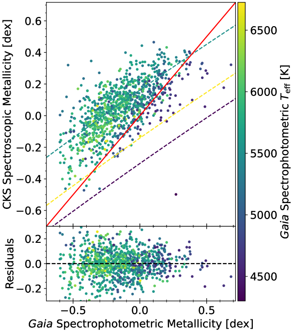
Figure 1: California-Kepler Survey (CKS, Petigura et al., 2017) spectroscopic metallicities versus those from Gaia DR3 spectrophotometry (Gaia Collaboration et al., 2022; Andrae et al., 2022; Creevey et al., 2022; Fouesneau et al., 2022). In the top panel, we plot a direct comparison between the CKS and Gaia metallicities, where the solid red line represents agreement and the colored curves show the best-fit polynomial relations used to correct Gaia metallicities for stars of different $T_{\mathrm{eff}}$. The bottom panel shows the residuals between the Gaia and CKS data after applying the corrections to the Gaia metallicities and the black-dashed line represents agreement. Row 1 of Table 1 contains the polynomial relation used to correct Gaia metallicities.

Table 1: CKS-Gaia Spectrophotometric Metallicites

Bounds	Adopted Metallicity
1. 4000 $<$ $T_{\mathrm{eff},G}$ $<$ 7000 K $\cap$ [M/H]G $>$ –2.0 dex	[Fe/H]adopt = –5.30 + 0.591 [M/H]G – 0.0257 [M/H]${}_{G}^{2}$ + 0.00193 $T_{\mathrm{eff},G}$ – 0.000000171 $T_{\mathrm{eff},G}^{2}$
2. Other	[Fe/H]adopt = 0.16 + 0.605 [M/H]G

Note. — CKS-based polynomial relations used to fix Gaia spectrophotometric metallicities. The $G$ denotes Gaia spectrophotometric parameters, while [Fe/H]_adopt represent our adopted metallicities. We plot the results of these relations in Figure 1.

To create a homogeneous catalog for the combined Kepler+K2+TESS host star samples, we used Gaia DR3 $G_{\mathrm{BP}}$ and $G_{\mathrm{RP}}$ as our photometric constraints. We chose these two passbands due to their mmag precision (Riello et al., 2021), color-$T_{\mathrm{eff}}$ sensitivity, and $G_{\mathrm{RP}}$’s relative insensitivity to extinction. The typical host star in our sample experiences $A_{V}$ = 0.15 mag, which we correct for with an extinction map. In addition, Gaia photometry has a $\lesssim$1” angular resolution (de Bruijne et al., 2015) compared to 2MASS’s 4” (Skrutskie et al., 2006), which minimizes issues of photometric blending. We used Riello et al. (2021) equations C.1-C.3 to correct saturated photometry, where relevant. While we did not modify the formal, $input$ uncertainties on the Gaia photometry, their mmag precision makes them difficult to use with a relatively sparse pre-computed grid like isoclassify uses; hence, we will detail the required modifications to isoclassify in §2.3.

In addition to the $G_{\mathrm{BP}}$ and $G_{\mathrm{RP}}$ photometry, we utilized Gaia DR3 parallaxes (Lindegren et al., 2021a) with zeropoint corrections (Lindegren et al., 2021b) and J2000 positions. Where possible, we used spectrophotometric metallicities (mh_gspphot, Creevey et al., 2022; Fouesneau et al., 2022; Andrae et al., 2022). Given that the spectrophotometric metallicities exhibit strong systematic errors (Andrae et al., 2022), we corrected them using California-Kepler Survey (CKS, Petigura et al., 2017) metallicities by fitting a quadratic polynomial as a function of spectrophotometric $T_{\mathrm{eff}}$ (teff_gspphot) and metallicity to the CKS metallicities. We only applied this relation to stars with Gaia spectrophotometric $T_{\mathrm{eff}}$ between 4000 and 7000 K and metallicities $>$–2.0 dex. For stars outside that range, we used a line representing the median offset between the Gaia spectrophotometric metallicities and the CKS. We display the CKS-Gaia metallicity comparison in Figure 1 and corresponding relations in Table 1. These homogeneous metallicities are available for a larger fraction of host stars, unlike the heterogeneous metallicities of LAMOST (Ren et al., 2018), APOGEE (Abolfathi et al., 2018), and the CKS (Petigura et al., 2017) used in Berger et al. (2020a).

Table 2 shows the parameters that we input into isoclassify. The metallicity provenance column can be one of three values: Poly, Med, or None. For stars with Poly provenances, we used the polynomial equation in row 1 of Table 1 and adopt an uncertainty of 0.15 dex as in Berger et al. (2020a) and for those with Med provenances (outside the $T_{\mathrm{eff}}$ and metallicity range of CKS stars), we used the linear equation in row 2 of Table 1 and adopt an uncertainty of 0.20 dex. These uncertainties are conservative by design, as Furlan et al. (2018) shows that systematic metallicity uncertainties between spectroscopic pipelines are typically $\geq$0.1 dex. Likewise, the scatter in the residuals of Figure 1 is $\approx$0.11 dex. Stars with None provenances lack Gaia DR3 spectrophotometric metallicities, and for these stars isoclassify defaults to a broad ($\gtrsim$0.20 dex), Gaussian solar metallicity prior.

Table 2: Gaia-Kepler-TESS-Host Stellar Input Parameters

Star ID	DR3 Source ID	$G_{\mathrm{BP}}$ [mag]	$G_{\mathrm{RP}}$ [mag]	$\pi$ [mas]	[Fe/H]	[Fe/H] Prov	RUWE
kic10858832	2129500383713365248	14.5940 $\pm$ 0.0030	13.7443 $\pm$ 0.0039	1.1711 $\pm$ 0.0135	0.200 $\pm$ 0.150	Poly	1.003
kic2571238	2051106987063242880	12.2374 $\pm$ 0.0028	11.3370 $\pm$ 0.0038	4.5680 $\pm$ 0.0087	0.137 $\pm$ 0.150	Poly	0.824
kic8628665	2126430409811576704	15.2767 $\pm$ 0.0031	14.4036 $\pm$ 0.0039	0.9280 $\pm$ 0.0185	0.072 $\pm$ 0.150	Poly	1.016
kic10328393	2130683904901068800	14.4843 $\pm$ 0.0032	13.3366 $\pm$ 0.0039	2.8866 $\pm$ 0.0133	-0.003 $\pm$ 0.150	Poly	1.010
epic210577548	44062348664673152	13.6642 $\pm$ 0.0029	12.4527 $\pm$ 0.0038	3.5165 $\pm$ 0.0151	-0.027 $\pm$ 0.150	Poly	0.939
epic220294712	2538769088655260416	12.5499 $\pm$ 0.0028	11.8115 $\pm$ 0.0038	2.3343 $\pm$ 0.0151	-0.092 $\pm$ 0.150	Poly	1.001
epic211711685	611385506505666688	12.7334 $\pm$ 0.0028	11.8419 $\pm$ 0.0038	3.4644 $\pm$ 0.0134	0.188 $\pm$ 0.150	Poly	0.944
epic251584580	3658535369882355712	14.8086 $\pm$ 0.0033	13.6446 $\pm$ 0.0041	2.6322 $\pm$ 0.0220	-0.289 $\pm$ 0.150	Poly	1.053
tic429501231	3423681228084838912	13.6640 $\pm$ 0.0032	12.7718 $\pm$ 0.0048	1.8895 $\pm$ 0.0285	-0.204 $\pm$ 0.150	Poly	1.533
tic255685030	5501542395359045504	11.4133 $\pm$ 0.0029	10.5290 $\pm$ 0.0038	6.3511 $\pm$ 0.0124	0.226 $\pm$ 0.150	Poly	0.990
tic238624131	378265951674712448	12.4537 $\pm$ 0.0028	11.5585 $\pm$ 0.0038	3.0227 $\pm$ 0.0132	0.188 $\pm$ 0.150	Poly	1.043
tic391903064	5212899427468919296	9.5947 $\pm$ 0.0075	8.7303 $\pm$ 0.0061	12.6898 $\pm$ 0.0105	0.154 $\pm$ 0.150	Poly	0.893

Note. — Star ID (kic for Kepler, epic for K2, and tic for TESS), Gaia DR3 source ID, $G_{\mathrm{BP}}$-mag, $G_{\mathrm{RP}}$-mag, parallax, metallicity, and metallicity provenance parameters and their uncertainties, which were provided as input to isoclassify. We also provide Gaia DR3 RUWE values for posterity. The [Fe/H] Prov column has three possible values: Poly, Med, and None. Poly values denote our use of the CKS-based polynomial method to fix the Gaia spectrophotometric metallicity (row 1 of Table 1), Med values denote our use of the median offset line (row 2 of Table 1), and None values denote stars that lack Gaia spectrophotometric metallicities, where isoclassify defaults to a broad, Gaussian solar metallicity prior. A subset of our input parameters is provided here to illustrate the form and format. The full table, in machine-readable format, can be found online.

2.3 Isochrone Fitting

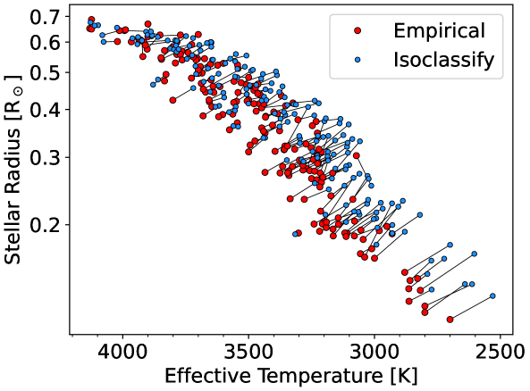
Figure 2: Stellar radius versus effective temperature for the Mann et al. (2015) M-dwarfs, where the red points represent the empirical data and the blue points are the isoclassify output using the plain PARSEC models (Bressan et al., 2012; Chen et al., 2019). We draw black lines connecting estimates for the same star. Because of this discrepancy, we use empirical corrections to constrain the properties of low mass stars.

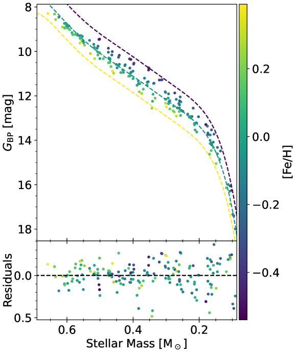
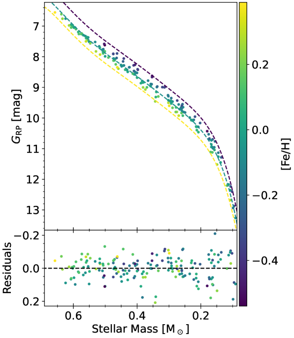
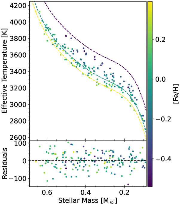
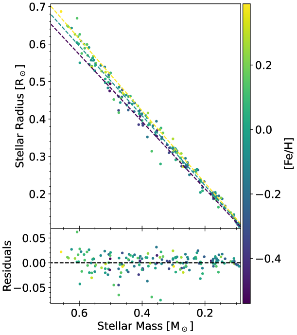
Figure 3: Empirical measurements (absolute $G_{\mathrm{BP}}$, absolute $G_{\mathrm{RP}}$, $T_{\mathrm{eff}}$, radius) versus stellar mass colored by metallicity for the Mann et al. (2015) sample of M-dwarfs. We derived the masses using the Mann et al. (2019) M_-M_K- code. Yellow, green, and indigo dashed lines show the best-fit relations for [Fe/H] = –0.6, 0.0, and 0.5 dex, and residuals show the observed values subtracted by the predicted value of the polynomial with a corresponding mass and metallicity, where the black dashed line indicates agreement. We include the numerical relations in Table 3.

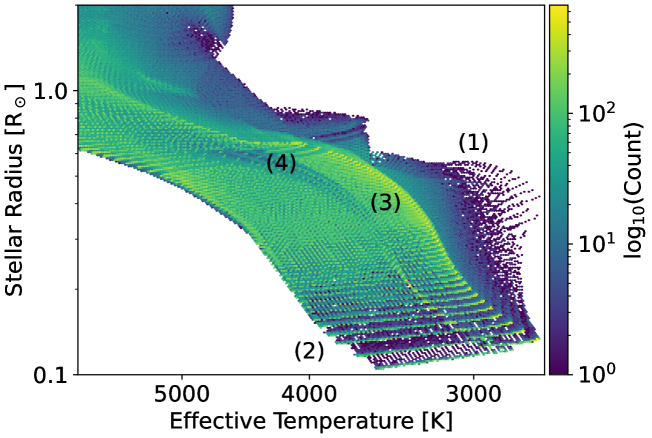
Figure 4: Stellar radius versus effective temperature for the empirically modified, interpolated PARSEC model grid utilized in this work. The logarithmic number density of models is represented by the color of each bin.

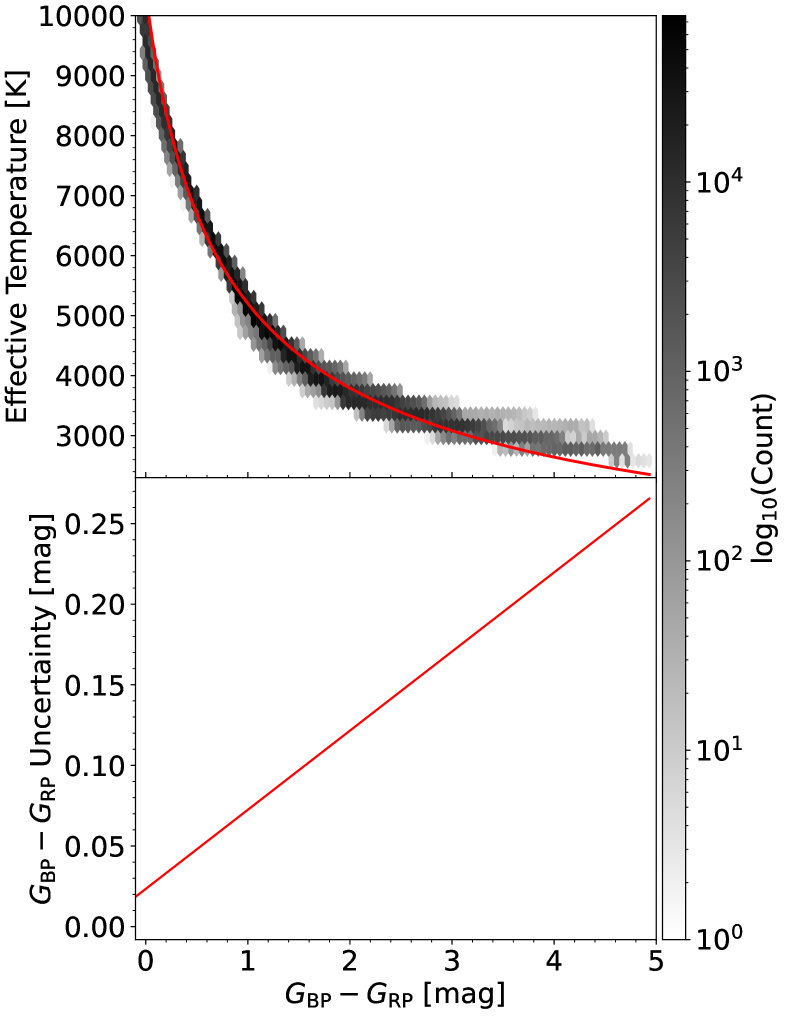
Figure 5: We place a floor on $G_{\mathrm{BP}}$–$G_{\mathrm{RP}}$ color uncertainties through our empirically modified PARSEC model grid. $Top$: $T_{\mathrm{eff}}$ versus $G_{\mathrm{BP}}$–$G_{\mathrm{RP}}$ color for our model grid, with the logarithmic density of points illustrated by the two-dimensional greyscale histogram with the corresponding colorbar. We plot our best-fit SmoothlyBrokenPowerLaw1D in red. $Bottom$: The red line represents the required $G_{\mathrm{BP}}$–$G_{\mathrm{RP}}$ minimum uncertainty to reach a 3% $T_{\mathrm{eff}}$ error for all stars, dependent on their $G_{\mathrm{BP}}$–$G_{\mathrm{RP}}$ color.

Table 3: Polynomial Empirical Relations for M-dwarfs

Parameter	Polynomial Empirical Relation
$G$	24.5898 – 183.9893 $\mathrm{M}_{\star}$ + 1120.1562 $\mathrm{M}^{2}_{\star}$ – 3770.5221 $\mathrm{M}^{3}_{\star}$ + 7016.0366 $\mathrm{M}^{4}_{\star}$ – 6804.3093 $\mathrm{M}^{5}_{\star}$ + 2672.7206 $\mathrm{M}^{6}_{\star}$ + 0.8813 [Fe/H]
$G_{\mathrm{BP}}$	34.4834 – 318.4227 $\mathrm{M}_{\star}$ + 2022.7769 $\mathrm{M}^{2}_{\star}$ – 6932.4997 $\mathrm{M}^{3}_{\star}$ + 13040.8749 $\mathrm{M}^{4}_{\star}$ – 12736.0413 $\mathrm{M}^{5}_{\star}$ + 5032.4396 $\mathrm{M}^{6}_{\star}$ + 1.4652 [Fe/H]
$G_{\mathrm{RP}}$	22.1215 – 165.2395 $\mathrm{M}_{\star}$ + 996.5293 $\mathrm{M}^{2}_{\star}$ – 3330.1792 $\mathrm{M}^{3}_{\star}$ + 6149.4185 $\mathrm{M}^{4}_{\star}$ – 5913.3984 $\mathrm{M}^{5}_{\star}$ + 2302.3600 $\mathrm{M}^{6}_{\star}$ + 0.6634 [Fe/H]
$T_{\mathrm{eff}}$	1352.4644 + 22894.5349 $\mathrm{M}_{\star}$ – 113739.3956 $\mathrm{M}^{2}_{\star}$ + 286679.2022 $\mathrm{M}^{3}_{\star}$ – 350226.7290 $\mathrm{M}^{4}_{\star}$ + 170350.2318 $\mathrm{M}^{5}_{\star}$ – 292.0425 [Fe/H] + 260.4901 [Fe/H]2
$R_{\star}$	(0.0361 + 0.9316 $\mathrm{M}_{\star}$) $\times$ (1 + 0.0638 [Fe/H])

Note. — Empirical relations for M-dwarfs based on stellar mass and metallicity. The PARSEC models are defined based on their masses and metallicities, so we compute empirical relations for the observables as a function of mass and metallicity. The Gaia photometric relations in this table are for absolute magnitudes, and the $T_{\mathrm{eff}}$ and radius relations were used to amend the $\log g$ and mean stellar densities of the models. These relations are only used for main sequence models with masses $<$ 0.63 $\mathrm{M}_{\odot}$ and metallicities $>$ –0.5 dex. We plot these relations in Figure 3. We also include Gaia $G$ for posterity.

In order to determine fundamental physical parameters from the input observables adopted from Gaia DR3, we used isoclassify (Huber et al., 2017; Berger et al., 2020a) in combination with a custom-interpolated PARSEC evolutionary model grid (Bressan et al., 2012). We used kiauhoku (Claytor et al., 2020) to finely interpolate the coarse models to 0.05 dex steps in metallicity between –2.0 to 0.5 dex, 117 masses between 0.1 and 5.0 $\mathrm{M}_{\odot}$, and ages between 0.01 Gyr and 30 Gyr. We used 100 equivalent evolutionary points (EEPs, Dotter, 2016) for the pre-main sequence, 250 for the main sequence, 100 for the subgiant branch, and 200 for the red giant branch up to the tip. We used YBC bolometric corrections (Chen et al., 2019) to compute synthetic photometry for our interpolated models.

Upon applying this grid to the sample of Mann et al. (2015, 2019) M-dwarfs crossmatched with Gaia photometry and parallaxes, we found large discrepancies between the measured physical parameters and those produced by our isochrone fitting analysis. Figure 2 shows that large systematics are present, and that the plain PARSEC grid produces systematically larger and cooler parameters for M-dwarfs than empirically measured. Therefore, we used the Mann et al. (2019) M_-M_K- code, which uses 2MASS $K_{s}$ magnitudes and Gaia parallaxes to compute stellar masses, to compute the empirical masses of the Mann et al. (2015) sample. Then, we used those masses and the spectroscopic metallicities tabulated in Mann et al. (2015) to compute polynomial empirical relations for Gaia $G$, $G_{\mathrm{BP}}$, $G_{\mathrm{RP}}$, stellar radius, and stellar effective temperature as a function of mass and metallicity. We used the Bayesian Information Criterion to determine the point at which adding additional parameters/changing the functional form no longer produced any significant benefit.

Figure 3 shows the Mann et al. (2015, 2019) data as a function of mass and colored by metallicity. In each of the diagrams, we do not see any strong trends in either the location or color of the residuals, showing that the mass-metallicity polynomials effectively describe the observational data. Table 3 contains the adopted numerical relations. For models within the mass and metallicity range of the Mann et al. (2015, 2019) data, we use each model’s mass and metallicity to replace the PARSEC $G_{\mathrm{BP}}$, $G_{\mathrm{RP}}$, $T_{\mathrm{eff}}$, $R_{\star}$, $\log g$, and mean stellar densities with values derived from the empirical polynomial fits displayed in Figure 3 and quantified in Table 3.

To ensure a smooth transition between the polynomial-modified models and the adjacent PARSEC models, we used a small range of masses and metallicities at which we weight the contribution of the empirical relations for those models. We defined this mass range as 0.63 $<$ $M_{\star}$ $<$ 0.70 $\mathrm{M}_{\odot}$, and the metallicity range as –0.65 $<$ [Fe/H] $<$ –0.50 dex, and computed the difference in the polynomial and evolutionary model predictions. We then scaled this difference based on the product of the mass and metallicity distance from 0.70 $\mathrm{M}_{\odot}$ and –0.65 dex, respectively, and added this difference to the PARSEC model for each parameter of interest. We chose these particular ranges because the Mann et al. (2015) sample includes stars with metallicities as low as $\approx$–0.6 dex and masses as large as $\approx$0.65 $\mathrm{M}_{\odot}$; we also wanted to avoid both (1) a sharp cutoff separating our empirical corrections and the pre-existing models and (2) an extended interpolation over a larger range of masses/metallicities.

Altogether, our modified PARSEC grid includes 2.8 million models, a portion of which is represented in Figure 4 as an HR diagram. This HR diagram includes a number of notable features: (1) pre-main sequence models for low-mass stars, which can be seen as the darker colored dots to the right of the main sequence, (2) model aliasing appearing as horizontal “strips” of low-mass stars on the main sequence due to computational limitations of the model grid size, (3) models with empirically modified parameters, which appear separated from the evolutionary models for low-mass main sequence stars, and (4) the transition region from empirical relations to evolutionary models.

We used isoclassify (Huber et al., 2017; Berger et al., 2020a) with the empirically modified PARSEC grid, Gaia DR3 $G_{\mathrm{BP}}$, $G_{\mathrm{RP}}$, parallaxes, positions, and metallicities, and the Combined19 map (Drimmel et al., 2003; Marshall et al., 2006; Green et al., 2019) within mwdust (Bovy et al., 2016) to correct for dust extinction and derive fundamental stellar parameters. Similar to Berger et al. (2020a), we also modified isoclassify to utilize uncertainties in $G_{\mathrm{BP}}$–$G_{\mathrm{RP}}$ that correspond to a $\sim$3% uncertainty in $T_{\mathrm{eff}}$ by fitting a smoothly broken power law (astropy’s SmoothlyBrokenPowerLaw1D) to the model grid’s $T_{\mathrm{eff}}$-$G_{\mathrm{BP}}$–$G_{\mathrm{RP}}$ relation. We chose the smoothly broken power law because it adequately fits the shape of the $T_{\mathrm{eff}}$-$G_{\mathrm{BP}}$–$G_{\mathrm{RP}}$ curve over the range of $T_{\mathrm{eff}}$ in the model grid with the fewest possible parameters, as compared to the 12th order polynomial fit in Berger et al. (2020a). We then divided the $T_{\mathrm{eff}}$ values by the derivative of this relation and multiplied by 3% to produce a $G_{\mathrm{BP}}$–$G_{\mathrm{RP}}$ uncertainty corresponding to 3% $T_{\mathrm{eff}}$ uncertainty. Finally, we computed the maximum of the derivative $G_{\mathrm{BP}}$–$G_{\mathrm{RP}}$ uncertainty and the measured $G_{\mathrm{BP}}$ and $G_{\mathrm{RP}}$ uncertainties added in quadrature as our adopted color uncertainty. Figure 5 shows this comparison and the corresponding power law-derived $T_{\mathrm{eff}}$ uncertainty. This ensures that we do not drastically underestimate $T_{\mathrm{eff}}$ uncertainties relative to the 2.0$\pm$0.5% $T_{\mathrm{eff}}$ systematic uncertainty floor of interferometry (Tayar et al., 2022) given the mmag precision of Gaia photometry and the imperfect power law fit to the model grid. For our stellar sample, we find that this procedure gives us a $\approx$2.4% $T_{\mathrm{eff}}$ uncertainty for solar-type stars.

3 Validating the Output Stellar Parameters

3.1 Accuracy of Derived Effective Temperatures, Radii, and Masses

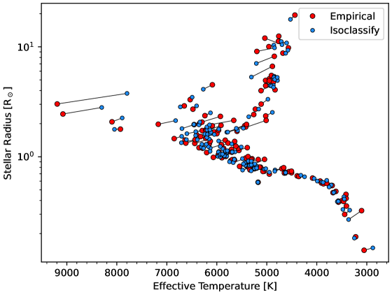
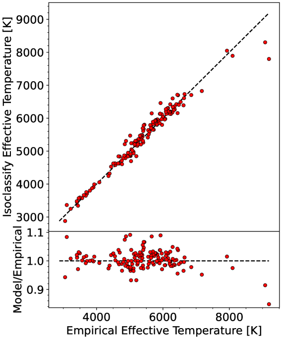
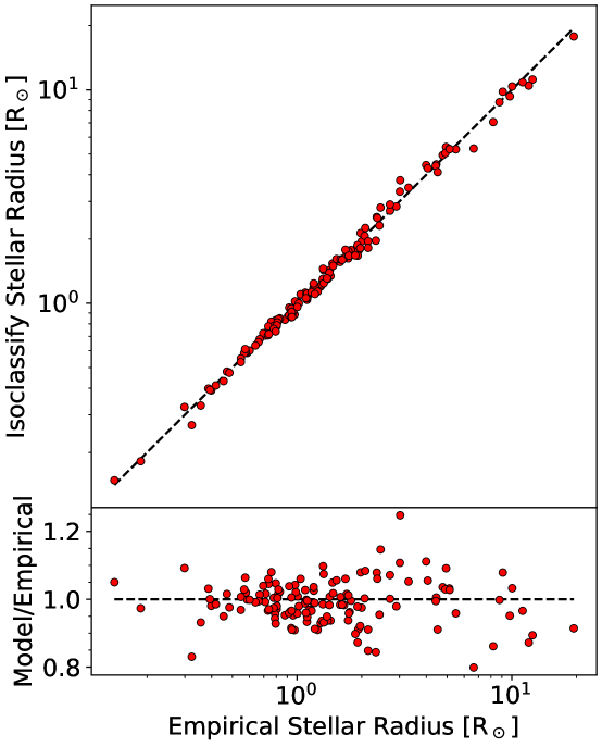
Figure 6: Interferometric $T_{\mathrm{eff}}$ and radius measurements versus isoclassify-derived results. $Top$: Radius versus $T_{\mathrm{eff}}$ diagram showing empirical measurements in red and isoclassify results in blue, where black lines connect the separate estimates for the same star. $Left$: Direct comparison of interferometric $T_{\mathrm{eff}}$ and isoclassify $T_{\mathrm{eff}}$. The black dashed line represents the 1:1 line and the bottom panel shows the corresponding fractional residuals. $Right$: Same as $Left$ but for stellar radius.

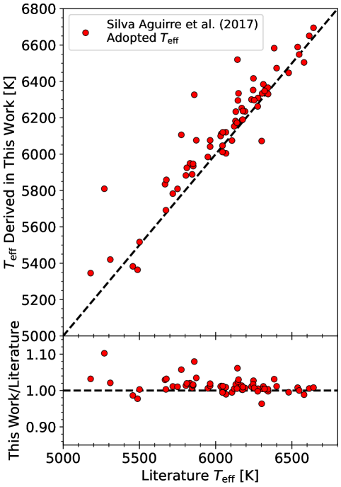
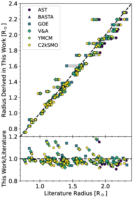
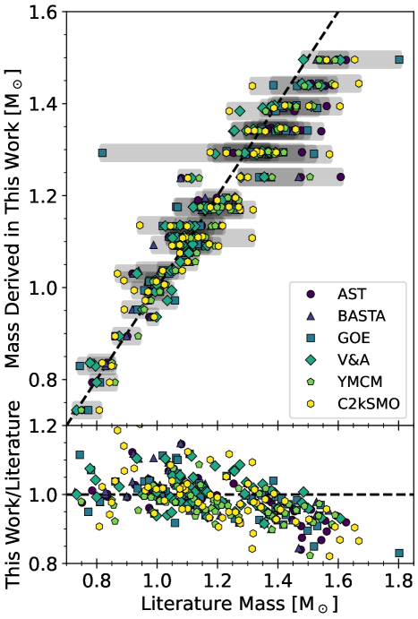
Figure 7: Effective temperatures, radii, and masses derived using our methodology versus those with frequency-modeled asteroseismic properties from a variety of pipelines (Silva Aguirre et al., 2017). The black dashed line represents agreement. The various colors/shapes represent the different pipelines. The translucent grey rounded rectangles represent the ranges of parameter estimates from different asteroseismic pipelines for each system, which includes not only seismic differences but also differences between model grids. The bottom panels show the ratio of the parameters derived in this work versus the single or multiple determinations of Silva Aguirre et al. (2017), which produces the curved residual structure apparent for each star in the right two plots.

To ensure our grid-computed stellar effective temperatures and radii are accurate, we compared them to interferometric $T_{\mathrm{eff}}$ and angular diameter measurements for a sample of 142 stars from Huber et al. (2012), Boyajian et al. (2013), White et al. (2018), Stokholm et al. (2019), Rains et al. (2020), and Karovicova et al. (2020, 2022a, 2022b). We followed a similar procedure as above to crossmatch to Gaia DR3 sources and correct the photometry and parallaxes for saturation and zeropoint differences, respectively. When we ran isoclassify, we did not correct for extinction given the interferometric sample’s proximity to Earth. Of the 142 stars, 118 are within 30 pc, 131 are within 60 pc, and only one (HD 6833) is beyond 200 pc.

Figure 6 shows comparisons of the interferometric stellar parameters and the isoclassify-derived stellar parameters. In general, we show agreement between the models and the interferometric estimates across the entire range of $T_{\mathrm{eff}}$ and radius, with residual offsets of 0.2% and 1.0% and residual scatters of 2.8% and 5.6%, compared to the median combined interferometric and isoclassify uncertainties of 2.6% and 4.6%, respectively. In addition, we find a systematic underestimation of $T_{\mathrm{eff}}$ for stars hotter than 9000 K. Since the distance to these stars is less than 30 pc, we can rule out extinction as a cause for this discrepancy. Upon further inspection, the Gaia DR3 photometry might be suspect for these objects, as the $G_{\mathrm{BP}}$–$G_{\mathrm{RP}}$ colors are much redder than their effective temperature, as the current version of the Pecaut & Mamajek (2013) table suggests. While the 0.2% and 1.0% differences between the scatter and median combined uncertainties are small, they suggest there are additional factors that could produce the excess scatter: (1) inaccurate photometry/parallaxes, (2) issues with the PARSEC models, and/or (3) issues with the YBC synthetic photometry.

In Figure 7 we compare our derived effective temperatures, radii, and masses to those of the Kepler LEGACY sample (Silva Aguirre et al., 2017), which includes estimates from a number of analysis pipelines for radii and masses. For $T_{\mathrm{eff}}$, radius, and mass, we find offsets of 0.9%, 1.8%, and 1.2% and residual scatters of 1.0%, 2.4%, and 5.0%, with differences between the individual pipelines producing offsets and scatters of similar or smaller size.

3.2 Accuracy of Derived Stellar Ages

3.2.1 Cluster Ages

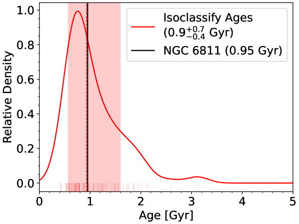
Figure 8: Age comparison for open cluster NGC 6811 at 0.95 Gyr (Godoy-Rivera et al., 2021), located within the Kepler field. The solid red distribution represents Gaussian Kernel Density Estimate (KDE) of the ages of individual stars within each cluster as derived in this work, with the median and the 1$\sigma$ confidence interval represented by the vertical red dashed line and shaded region, respectively. We use Scott’s rule (Scott, 1992) bandwidths to produce the overall distribution. Translucent vertical red lines represent the inferred ages for each star within the sample. The black, solid vertical line represents the cluster ages from the literature in each panel. We only include stars with $T_{\mathrm{eff}}$ $>$ 6000 K and RUWE $<$ 1.4.

To independently confirm our derived stellar ages, we used the NGC 6811 cluster data from Godoy-Rivera et al. (2021). We followed a similar procedure as above to crossmatch the NGC 6811 members found by Godoy-Rivera et al. (2021) to Gaia DR3 sources and perform corrections to the parallaxes and photometry, where necessary. We then removed stars not classified as probable members and those without Gaia DR3 solutions, leaving us with 338 stars. We used the Godoy-Rivera et al. (2021) NGC 6811 metallicity ([Fe/H] = 0.03 dex) with 0.15 dex uncertainties for each member, and when we ran isoclassify, we used the mwdust allsky extinction map as above. To ensure that our derived isochrone ages are reliable and minimize the potential for age contaminating binaries (Berger et al., 2020a), we removed all stars with $T_{\mathrm{eff}}$ $<$ 6000 K and RUWE $>$ 1.4 (Stassun & Torres, 2021). For the remaining 107 stars, we compared stellar ages.

Figure 8 shows our derived ages for individual stars and their ensemble age versus the Godoy-Rivera et al. (2021) NGC 6811 cluster age (0.95 Gyr). Our age distribution is in agreement with the cluster’s age. Similar to Berger et al. (2020a), there are a few stars at ages $>$2 Gyr. After plotting the 107 NGC 6811 stars in an HR diagram, we find that the $>$2 Gyr stars are also the coolest and largest subgiants remaining. Although we already removed stars with RUWE $>$ 1.4, some of these members might have very close unresolved companions (Stassun & Torres, 2021) that are less massive and cooler, which can bias our results towards older ages (Berger et al., 2020a).

3.2.2 Asteroseismic Ages

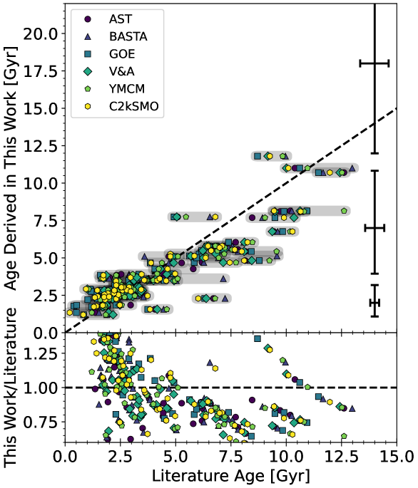
Figure 9: Ages derived using our methodology versus those with frequency-modeled asteroseismic ages from a variety of pipelines (Silva Aguirre et al., 2017). The black dashed line represents agreement. The various colors/shapes represent the different pipelines. The translucent grey rounded rectangles represent the ranges of age estimates from different asteroseismic pipelines for each system, which includes not only seismic differences but also differences between model grids. The bottom panel is the ratio of the age derived in this work versus the multiple determinations of Silva Aguirre et al. (2017), which produces the curved residual structure apparent for each star. We have also plotted median error bars in the right-hand portion of the top panel, where, from bottom to top, the error bars represent the median uncertainties of stars with isochrone ages between 0–4 Gyr, 4–8 Gyr, and $>$8 Gyr, respectively.

We also compared our derived ages to those of Kepler stars that have asteroseismic ages as in Berger et al. (2020a). We utilized the “boutique” frequency-modeled ages from the Kepler legacy sample detailed in Silva Aguirre et al. (2017), which includes results from a number of analysis pipelines. In Figure 9, the ages that we derive are in reasonable agreement with those provided by a variety of asteroseismic pipelines. The horizontal scatter of the colored points are typically larger than their reported errors, which indicates that systematic pipeline differences dominate. Any deviations from the 1:1 dashed line are sufficiently accounted for by a combination of the typical error bars (bottom right, top panel) and any systematic scatter depending on the asteroseismic pipeline one chooses. The structure in the residuals in the bottom panel results from their representation as a ratio between the age derived in this work and those of Silva Aguirre et al. (2017). In addition, the asteroseismic ages do not fall above the age of the Universe (likely due to a model grid age-cutoff). We also see that at intermediate ages (4–8 Gyr), we may slightly underestimate stellar ages, but our solutions are well-within our reported uncertainties.

Ultimately, we report a median offset and scatter of 0.7% and 31% between our isochrone-derived ages and the asteroseismic ages of Silva Aguirre et al. (2017), respectively. We conclude that our isochrone-derived ages are consistent with ages determined through more precise methods within the uncertainties that we report.

4 Results

4.1 Stellar Properties

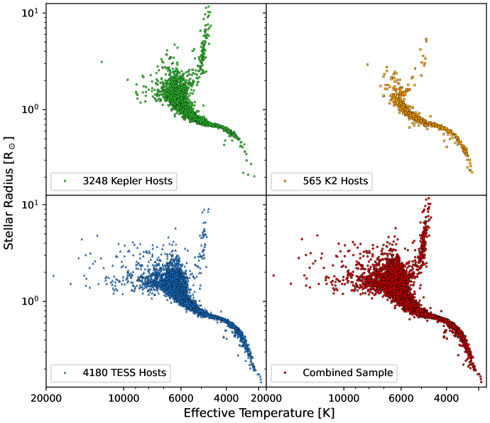
Figure 10: Stellar radius versus effective temperature for the Kepler, K2, TESS, and combined host star samples.

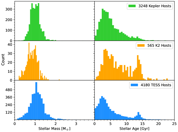
Figure 11: Histograms of masses and ages for the Kepler, K2, and TESS host star samples, where the left column contains stellar masses and the right column contains stellar ages. The Kepler, K2, and TESS, samples are displayed in each row and ordered, respectively, from top to bottom.

We present our homogeneous stellar properties in Table 4 and Figure 10. Figure 10 shows the host star populations broken up into separate panels for each mission and the combined host star sample in the bottom right. Most Kepler host stars are solar-like stars, as was the priority of the Kepler mission’s target selection (Borucki et al., 2010; Batalha et al., 2010) and as has been confirmed more recently thanks to Gaia photometry and parallaxes (Wolniewicz et al., 2021). Of the 3248 Kepler host stars, only 17 are hotter than 8000 K, while 95 are cooler than 4000 K. Relative to the K2 and TESS host stars, there are more giants with planet candidates in the Kepler host star sample. This is likely because of Kepler’s superior sensitivity and baseline when compared to the shorter continuous baselines and increased systematic noise/smaller apertures of K2/TESS.

The upper right panel of Figure 10 displays the K2 host star sample. There are fewer K2 hosts than both Kepler and TESS, mostly because we used the homogeneously derived input sample from Zink et al. (2021). Due to differences in target selection, most K2 host stars are lower mass than those observed by Kepler. Eighty-nine K2 stars are cooler than 4000 K and 216 are cooler than 5000 K, as K2 target selection was community-led and prioritized K and M-dwarfs in its search for planets (Dressing & Charbonneau, 2013; Howell et al., 2014; Dressing & Charbonneau, 2015; Huber et al., 2016b; Cloutier & Menou, 2020). Only one star in our K2 sample is hotter than 8000 K. In the lower left panel, we plot the TESS host star distribution. TESS host stars, perhaps unsurprisingly, contain the largest diversity of stellar types, given TESS’s all-sky observations. Host stars range in $T_{\mathrm{eff}}$ from 2934 K up to 18740 K, and of the 4180 hosts, 317 are cooler than 4000 K and 179 are hotter than 8000 K. However, we caution that a large fraction ($\approx$85%) of the TESS host stars are hosts to planet candidates and hence have not been subject to the scrutiny of ground-based follow-up or comprehensive vetting routines.

Together, our Kepler+K2+TESS host star sample, displayed in the bottom right panel of Figure 10, represents both the largest and most diverse transiting exoplanet host star sample with homogeneous fundamental parameters yet. This enables a direct comparison of the host stars and their stellar properties and the construction of larger host samples across a wide range of parameter space. For instance, we count 492 host stars with $T_{\mathrm{eff}}$ $>$ 6000 K and isochrone ages $<$1 Gyr. These stars represent an interesting sample for further study, although we note the potential for many of the planet candidates orbiting these stars, especially those $>$ 10000 K, to be false positives. The ages of exoplanet host stars are particularly useful for determining how exoplanets evolve over time (Soderblom, 2010; Mann et al., 2017; Berger et al., 2018a, 2020b, 2022; David et al., 2021).

We plot the distribution of masses and ages in Figure 11. As is clear in Figure 10, the mass (and age) ranges vary from sample to sample, where Kepler host stars are mostly close to one solar mass, while K2 hosts shift to lower masses and TESS hosts include a broader distribution of stellar masses. In stellar age, we see that the Kepler and K2 distributions are similar except for the peak in stellar age between 13 and 15 Gyr - this is because K2 focused more heavily on low-mass K and M-dwarfs, which do not produce meaningful isochrone ages and tend to have ages roughly half the maximum age of our model grid (30 Gyr). The TESS histogram displays a large number of hosts younger than 3 Gyr, most of which are stars in the high mass tail of the TESS mass histogram.

4.2 Exoplanet Properties

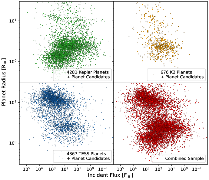
Figure 12: Planet radius versus incident flux for the Kepler, K2, and TESS, and combined planet samples. While most planets are shown, there are 1 Kepler and 68 TESS planets that experience incident fluxes $<$ 0.01 $\mathrm{F_{\oplus}}$.

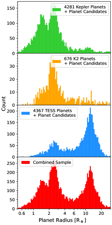
Figure 13: Planet radius histograms for the Kepler, K2, and TESS, and combined planet samples.

As in Berger et al. (2020b), we utilized the Cumulative KOI table at the NASA Exoplanet Archive (Batalha et al., 2013; Burke et al., 2014; Rowe et al., 2015; Mullally et al., 2015; Coughlin et al., 2016; Thompson et al., 2018; NASA Exoplanet Archive, 2021) catalog-provided $R_{\mathrm{p}}/R_{\star}$ and orbital period values, where available, in combination with our stellar parameters and their uncertainties to compute planet radii, semimajor axes, and incident fluxes. Both the Cumulative KOI and Zink et al. (2021) catalogs provide $R_{\mathrm{p}}/R_{\star}$ values for the Kepler and K2 planet samples, but the TESS Project Candidate table (e.g. Guerrero et al., 2021) at the NASA Exoplanet Archive does not. Therefore, we used this TESS table’s stellar and planet radii to compute $R_{\mathrm{p}}/R_{\star}$ which we then multiplied by our stellar radii to compute TESS planet radii. We do not use transit depth measurements to compute TESS planet radii because transit depth measurements do not directly translate into planetary radii for planets that have large impact parameters.

We present our planet properties in Table 5 and Figure 12. Similar to the stellar populations in §4.1, the planet populations in the planet radius-incident flux diagrams differ from panel-to-panel. In the upper left panel containing Kepler planets, we can see a few, clear sub-populations of planets. We see two populations of planets smaller than 5 $\mathrm{R_{\oplus}}$, separated at by the planet radius gap at $\sim$2 $\mathrm{R_{\oplus}}$: these are the super-Earths ($\lesssim$2 $\mathrm{R_{\oplus}}$) and sub-Neptunes ($\gtrsim$2 $\mathrm{R_{\oplus}}$and $\lesssim$4 $\mathrm{R_{\oplus}}$), as identified by Fulton et al. (2017). There are many super-Earths due to Kepler’s sensitivity and baseline, and the sub-Neptune population appears to be well-defined given the drop-off in planets at $>$5 $\mathrm{R_{\oplus}}$. Finally, we observe a group of Jupiter-sized planets (10–20 $\mathrm{R_{\oplus}}$) at a wide range of incident fluxes.

We show the K2 planet population in the upper right panel of Figure 12. There are far fewer K2 planets than in either Kepler or TESS, and while we see the sub-Neptune population, K2 did not detect many super-Earths. Hence, the planet radius gap is not clear in the K2 sample due to the small number of super-Earths, although it was detected in Hardegree-Ullman et al. (2020) and Zink et al. (2021). The differences in planet radii must come from the utilized stellar radii; we used the same $R_{\mathrm{p}}/R_{\star}$ values as Zink et al. (2021) but used a predominantly photometric isochrone fitting approach as compared to the spectroscopically-dependent random forest classifier of Hardegree-Ullman et al. (2020). Comparing the two sets of stellar radii, we find a median offset of $\approx$3% and typical scatter of $\approx$5% with some larger outliers. The observation that the K2 planet radius gap can disappear because of a statistically consistent yet slightly different set of stellar parameters suggests it is not yet robustly determined, unlike the Kepler planet radius gap.

We plot the TESS planets in the bottom left panel, and while there are more TESS planets than Kepler planets, Kepler has more super-Earths and sub-Neptunes. The vast majority of TESS planets are hot Jupiters, which appear to become more inflated at higher incident flux (Miller & Fortney, 2011; Thorngren et al., 2016; Grunblatt et al., 2016, 2017, 2019), although TESS has also detected quite a few sub-Neptunes. Due to its shorter observation baselines and reduced sensitivity relative to Kepler (Ricker et al., 2014), TESS has not detected as many super-Earths. Hence, we do not see a clear gap separating super-Earths and sub-Neptunes. One explanation for the lack of a clear gap in both the K2 and TESS samples are their less-precise $R_{\mathrm{p}}/R_{\star}$ values (Petigura, 2020). As above, we caution that a large fraction of the TESS planets are planet candidates and upon follow-up some number will be identified as false-positives.

The combined planet sample in the bottom right panel of Figure 12 represents the largest transiting exoplanet sample with homogeneously derived planet parameters yet. This enables us to increase the number of planets in notable regions of parameter space, such as the hot sub-Neptunian desert ($R_{\mathrm{p}}$ = 2.2–3.8 $\mathrm{R_{\oplus}}$ and $F_{\mathrm{p}}$ $>$ 650 $\mathrm{F_{\oplus}}$, Lundkvist et al., 2016; Berger et al., 2018b, 2020b), the habitable zone ($F_{\mathrm{p}}$ = 0.25–1.50 $\mathrm{F_{\oplus}}$, Kane et al., 2016; Berger et al., 2018b, 2020b), and the planet radius gap (Fulton et al., 2017; Fulton & Petigura, 2018; Van Eylen et al., 2018; Berger et al., 2018b, 2020b; Petigura, 2020; Petigura et al., 2022). Moreover, the populations of inflated Jupiters, both hot and warm/cold (Berger et al., 2018b, 2020b), warrant additional scrutiny.

We take a closer look at the Kepler, K2, TESS, and combined planet radius histograms in Figure 13. Similar to our conclusions based on the various panels in Figure 12, we see no clear gap in either the K2 or TESS planet radius histograms. We emphasize that these are raw numbers and are not completeness-corrected. Comparing the Kepler and combined samples, it is clear that Kepler provides superior gap resolution, and the addition of K2 and TESS planets makes it less-clear.

5 Conclusion

We presented the Gaia-Kepler-TESS-Host Stellar Properties Catalog and the corresponding catalog of homogeneous exoplanet properties, which contain 7993 stars and 9324 planets, respectively. We used isoclassify and Gaia DR3 to compute precise, homogeneous $T_{\mathrm{eff}}$, $\log g$, masses, radii, mean stellar densities, luminosities, ages, distances, and V-band extinctions for 3248, 565, and 4180 Kepler, K2, and TESS stars, respectively. We compared our stellar properties to studies using fundamental and precise constraints, such as interferometry and asteroseismology, and find good agreement between our $T_{\mathrm{eff}}$, radii, and ages and those in the literature. In addition, we provide planet radii, semimajor axes, and incident fluxes for 4281, 676, and 4367 Kepler, K2, and TESS planets, respectively, and find that the exoplanet radius gap is less prominent in K2 and TESS and combined samples than it is in the Kepler sample alone. We provide our stellar and planet catalogs as machine-readable tables associated with this article and as a High-Level Science Product (HLSP) at the Mikulski Archive for Space Telescopes (MAST). Finally, we identify over 1000 hot Jupiter planet candidates, 150 planets within the hot sub-Neptunian desert, and more than 400 young host stars as potential opportunities for testing the theories of planet formation and evolution.

Exoplanet Archive

Table 4: Gaia-Kepler-TESS-Host Stellar Output Parameters

Star ID	$T_{\mathrm{eff}}$ [K]	$\log g$ [dex]	[Fe/H]	$M_{\star}$ [$\mathrm{M_{\odot}}$]	$R_{\star}$ [$\mathrm{R_{\odot}}$]	$\rho_{\star}$ [$\mathrm{\rho_{\odot}}$]	$L_{\star}$ [$\mathrm{L_{\odot}}$]	Age [Gyr]	Distance [pc]	$A_{V}$ [mag]
kic10858832	5812${}^{+106}_{-124}$	4.424${}^{+0.035}_{-0.058}$	0.140${}^{+0.131}_{-0.138}$	1.054${}^{+0.042}_{-0.061}$	1.040${}^{+0.041}_{-0.030}$	0.927${}^{+0.103}_{-0.146}$	1.122${}^{+0.048}_{-0.045}$	2.86${}^{+3.75}_{-2.17}$	853.5${}^{+15.4}_{-15.0}$	0.110
kic2571238	5444${}^{+99}_{-110}$	4.510${}^{+0.033}_{-0.058}$	0.055${}^{+0.139}_{-0.135}$	0.915${}^{+0.043}_{-0.056}$	0.880${}^{+0.035}_{-0.026}$	1.334${}^{+0.142}_{-0.211}$	0.620${}^{+0.019}_{-0.019}$	4.29${}^{+6.25}_{-3.33}$	218.9${}^{+3.1}_{-3.0}$	0.000
kic8628665	5895${}^{+113}_{-122}$	4.450${}^{+0.030}_{-0.051}$	-0.021${}^{+0.135}_{-0.131}$	1.034${}^{+0.038}_{-0.059}$	1.000${}^{+0.037}_{-0.030}$	1.024${}^{+0.103}_{-0.144}$	1.093${}^{+0.062}_{-0.058}$	2.31${}^{+3.43}_{-1.79}$	1079.5${}^{+26.2}_{-25.5}$	0.275
kic10328393	4818${}^{+84}_{-106}$	4.596${}^{+0.033}_{-0.058}$	-0.092${}^{+0.140}_{-0.135}$	0.735${}^{+0.041}_{-0.039}$	0.715${}^{+0.024}_{-0.023}$	2.001${}^{+0.221}_{-0.304}$	0.250${}^{+0.008}_{-0.010}$	*7.98${}^{+11.15}_{-6.15}$	346.7${}^{+5.1}_{-5.0}$	0.027
epic210577548	5381${}^{+114}_{-121}$	4.531${}^{+0.038}_{-0.066}$	-0.098${}^{+0.136}_{-0.135}$	0.854${}^{+0.040}_{-0.059}$	0.829${}^{+0.037}_{-0.029}$	1.486${}^{+0.186}_{-0.260}$	0.525${}^{+0.017}_{-0.016}$	5.61${}^{+8.01}_{-4.34}$	284.3${}^{+4.3}_{-4.1}$	0.604
epic220294712	6294${}^{+135}_{-153}$	4.360${}^{+0.037}_{-0.056}$	-0.127${}^{+0.121}_{-0.144}$	1.132${}^{+0.044}_{-0.060}$	1.159${}^{+0.047}_{-0.035}$	0.718${}^{+0.085}_{-0.111}$	1.915${}^{+0.085}_{-0.080}$	1.88${}^{+2.31}_{-1.37}$	428.0${}^{+6.6}_{-6.4}$	0.192
epic211711685	5484${}^{+95}_{-106}$	4.496${}^{+0.033}_{-0.059}$	0.111${}^{+0.132}_{-0.138}$	0.936${}^{+0.040}_{-0.044}$	0.906${}^{+0.036}_{-0.026}$	1.256${}^{+0.132}_{-0.199}$	0.676${}^{+0.022}_{-0.021}$	4.00${}^{+5.78}_{-3.09}$	288.7${}^{+4.2}_{-4.1}$	0.000
epic251584580	4830${}^{+133}_{-242}$	4.601${}^{+0.044}_{-0.064}$	-0.352${}^{+0.128}_{-0.123}$	0.696${}^{+0.021}_{-0.042}$	0.686${}^{+0.028}_{-0.025}$	2.103${}^{+0.304}_{-0.355}$	0.233${}^{+0.014}_{-0.030}$	*9.59${}^{+11.13}_{-7.18}$	379.8${}^{+6.2}_{-5.9}$	0.137
tic429501231	5779${}^{+164}_{-188}$	4.371${}^{+0.073}_{-0.082}$	-0.186${}^{+0.134}_{-0.150}$	0.914${}^{+0.080}_{-0.081}$	1.025${}^{+0.060}_{-0.049}$	0.828${}^{+0.199}_{-0.178}$	1.073${}^{+0.055}_{-0.051}$	8.01${}^{+6.05}_{-5.06}$	527.8${}^{+11.3}_{-11.1}$	0.110
tic255685030	5519${}^{+91}_{-98}$	4.502${}^{+0.028}_{-0.050}$	0.120${}^{+0.131}_{-0.138}$	0.957${}^{+0.037}_{-0.045}$	0.909${}^{+0.031}_{-0.024}$	1.270${}^{+0.114}_{-0.174}$	0.696${}^{+0.023}_{-0.021}$	3.16${}^{+4.84}_{-2.47}$	157.5${}^{+2.2}_{-2.2}$	0.053
tic238624131	5924${}^{+115}_{-141}$	4.384${}^{+0.041}_{-0.062}$	0.148${}^{+0.130}_{-0.143}$	1.096${}^{+0.057}_{-0.062}$	1.110${}^{+0.048}_{-0.033}$	0.792${}^{+0.101}_{-0.133}$	1.376${}^{+0.053}_{-0.049}$	2.84${}^{+3.39}_{-2.12}$	330.6${}^{+4.9}_{-4.8}$	0.247
tic391903064	5721${}^{+107}_{-126}$	4.451${}^{+0.035}_{-0.059}$	0.088${}^{+0.140}_{-0.133}$	1.012${}^{+0.044}_{-0.060}$	0.987${}^{+0.039}_{-0.028}$	1.038${}^{+0.117}_{-0.163}$	0.950${}^{+0.034}_{-0.032}$	3.30${}^{+4.48}_{-2.51}$	78.8${}^{+1.1}_{-1.1}$	0.089

Note. — KIC ID, effective temperature, surface gravity, surface metallicity, stellar mass, stellar radius, density, luminosity, age, distance, and $V$-magnitude extinction, output from our isochrone fitting routine detailed in §2. Asterisks are appended to stellar ages that are uninformative ($T_{\mathrm{eff}}$ $<$ 5000 K). A subset of our output parameters is provided here to illustrate the form and format. The full table, in machine-readable format, can be found online.

Table 5: Gaia-Kepler-TESS Planet Parameters

Star ID	Planet ID	Disposition	$P$ [days]	$R_{\mathrm{p}}/R_{\star}$	$R_{\mathrm{p}}$ [$\mathrm{R_{\oplus}}$]	$a$ [AU]	$F_{\mathrm{p}}$ [$\mathrm{F_{\oplus}}$]
kic10797460	K00752.01	CP	9.488036${}^{+0.000028}_{-0.000028}$	0.02234${}^{+0.00083}_{-0.00053}$	2.20${}^{+0.12}_{-0.09}$	0.08577${}^{+0.00119}_{-0.00182}$	99.190${}^{+8.149}_{-7.296}$
kic10797460	K00752.02	CP	54.418383${}^{+0.000248}_{-0.000248}$	0.02795${}^{+0.00908}_{-0.00135}$	2.76${}^{+0.90}_{-0.16}$	0.27482${}^{+0.00381}_{-0.00584}$	9.661${}^{+0.794}_{-0.711}$
kic10811496	K00753.01	PC	19.899140${}^{+0.000015}_{-0.000015}$	0.15405${}^{+5.03429}_{-0.04218}$	18.82${}^{+615.00}_{-5.23}$	0.14628${}^{+0.00290}_{-0.00369}$	61.417${}^{+5.571}_{-5.550}$
kic10854555	K00755.01	CP	2.525592${}^{+0.000004}_{-0.000004}$	0.02406${}^{+0.00375}_{-0.00152}$	2.42${}^{+0.40}_{-0.18}$	0.03550${}^{+0.00053}_{-0.00080}$	629.842${}^{+46.532}_{-48.596}$
epic201155177	epic201155177.01	KP	6.689040${}^{+0.000796}_{-0.000871}$	0.02850${}^{+0.00100}_{-0.00100}$	2.15${}^{+0.09}_{-0.10}$	0.06105${}^{+0.00109}_{-0.00123}$	49.117${}^{+3.183}_{-4.935}$
epic201208431	epic201208431.01	KP	10.004208${}^{+0.000881}_{-0.000858}$	0.03520${}^{+0.00100}_{-0.00100}$	2.47${}^{+0.09}_{-0.09}$	0.07737${}^{+0.00086}_{-0.00086}$	17.275${}^{+1.036}_{-0.857}$
epic201247497	epic201247497.01	PC	2.754012${}^{+0.000122}_{-0.000132}$	0.09170${}^{+0.02800}_{-0.01900}$	6.82${}^{+2.09}_{-1.43}$	0.03339${}^{+0.00040}_{-0.00066}$	116.013${}^{+15.740}_{-14.916}$
epic201295312	epic201295312.01	KP	5.656766${}^{+0.000276}_{-0.000323}$	0.01710${}^{+0.00000}_{-0.00000}$	2.73${}^{+0.14}_{-0.13}$	0.06523${}^{+0.00160}_{-0.00146}$	567.312${}^{+36.131}_{-32.633}$
tic88863718	toi1001.01	PC	1.931671${}^{+0.000008}_{-0.000008}$	0.04701${}^{+0.01480}_{-0.01480}$	10.05${}^{+3.20}_{-3.20}$	0.03351${}^{+0.00039}_{-0.00045}$	7303.777${}^{+360.938}_{-354.659}$
tic65212867	toi1007.01	PC	6.998921${}^{+0.000014}_{-0.000014}$	0.05012${}^{+0.00354}_{-0.00354}$	14.40${}^{+1.22}_{-1.22}$	0.08440${}^{+0.00097}_{-0.00158}$	1506.786${}^{+71.140}_{-80.125}$
tic231663901	toi101.01	KP	1.430369${}^{+0.000001}_{-0.000001}$	0.13623${}^{+0.00954}_{-0.00954}$	13.23${}^{+1.04}_{-1.00}$	0.02429${}^{+0.00031}_{-0.00054}$	1301.559${}^{+59.105}_{-73.562}$
tic114018671	toi1011.01	PC	2.469696${}^{+0.000579}_{-0.000579}$	0.01415${}^{+0.01856}_{-0.01856}$	1.38${}^{+1.82}_{-1.82}$	0.03468${}^{+0.00055}_{-0.00099}$	547.740${}^{+24.947}_{-35.398}$

Note. — Host star ID, planet ID, disposition, orbital period, $R_{\mathrm{p}}/R_{\star}$, planet radius, semimajor axis, and incident flux values and their uncertainties for all planets contained within our catalog. Dispositions are designated as KP, CP, PC, APC, or LPPC for Known Planet, Confirmed Planet, Planetary Candidate, Ambiguous Planetary Candidate, or Long Period Planetary Candidate, respectively. A subset of our planet parameters is provided here to illustrate the form and format. The full table, in machine-readable format, can be found online.

References

- Abolfathi et al. (2018) Abolfathi, B., Aguado, D. S., Aguilar, G., et al. 2018, ApJS, 235, 42, doi: 10.3847/1538-4365/aa9e8a
- Andrae et al. (2022) Andrae, R., Fouesneau, M., Sordo, R., et al. 2022, arXiv e-prints, arXiv:2206.06138. https://arxiv.org/abs/2206.06138
- Astropy Collaboration et al. (2013) Astropy Collaboration, Robitaille, T. P., Tollerud, E. J., et al. 2013, A&A, 558, A33, doi: 10.1051/0004-6361/201322068
- Astropy Collaboration et al. (2018) Astropy Collaboration, Price-Whelan, A. M., Sipőcz, B. M., et al. 2018, AJ, 156, 123, doi: 10.3847/1538-3881/aabc4f
- Astropy Collaboration et al. (2022) Astropy Collaboration, Price-Whelan, A. M., Lim, P. L., et al. 2022, ApJ, 935, 167, doi: 10.3847/1538-4357/ac7c74
- Babusiaux et al. (2022) Babusiaux, C., Fabricius, C., Khanna, S., et al. 2022, arXiv e-prints, arXiv:2206.05989. https://arxiv.org/abs/2206.05989
- Batalha et al. (2010) Batalha, N. M., Borucki, W. J., Koch, D. G., et al. 2010, ApJ, 713, L109, doi: 10.1088/2041-8205/713/2/L109
- Batalha et al. (2013) Batalha, N. M., Rowe, J. F., Bryson, S. T., et al. 2013, ApJS, 204, 24, doi: 10.1088/0067-0049/204/2/24
- Berger et al. (2018a) Berger, T. A., Howard, A. W., & Boesgaard, A. M. 2018a, ApJ, 855, 115, doi: 10.3847/1538-4357/aab154
- Berger et al. (2018b) Berger, T. A., Huber, D., Gaidos, E., & van Saders, J. L. 2018b, ApJ, 866, 99, doi: 10.3847/1538-4357/aada83
- Berger et al. (2020a) Berger, T. A., Huber, D., van Saders, J. L., et al. 2020a, AJ, 159, 280, doi: 10.3847/1538-3881/159/6/280
- Berger et al. (2020b) Berger, T. A., Huber, D., Gaidos, E., van Saders, J. L., & Weiss, L. M. 2020b, AJ, 160, 108, doi: 10.3847/1538-3881/aba18a
- Berger et al. (2022) Berger, T. A., van Saders, J. L., Huber, D., et al. 2022, arXiv e-prints, arXiv:2206.10624. https://arxiv.org/abs/2206.10624
- Borucki et al. (2010) Borucki, W. J., Koch, D., Basri, G., et al. 2010, Science, 327, 977, doi: 10.1126/science.1185402
- Bovy et al. (2016) Bovy, J., Rix, H.-W., Green, G. M., Schlafly, E. F., & Finkbeiner, D. P. 2016, ApJ, 818, 130, doi: 10.3847/0004-637X/818/2/130
- Boyajian et al. (2013) Boyajian, T. S., von Braun, K., van Belle, G., et al. 2013, ApJ, 771, 40, doi: 10.1088/0004-637X/771/1/40
- Bressan et al. (2012) Bressan, A., Marigo, P., Girardi, L., et al. 2012, MNRAS, 427, 127, doi: 10.1111/j.1365-2966.2012.21948.x
- Burke et al. (2014) Burke, C. J., Bryson, S. T., Mullally, F., et al. 2014, ApJS, 210, 19, doi: 10.1088/0067-0049/210/2/19
- Chen et al. (2019) Chen, Y., Girardi, L., Fu, X., et al. 2019, A&A, 632, A105, doi: 10.1051/0004-6361/201936612
- Ciceri et al. (2015) Ciceri, S., Lillo-Box, J., Southworth, J., et al. 2015, A&A, 573, L5, doi: 10.1051/0004-6361/201425145
- Claytor et al. (2020) Claytor, Z. R., van Saders, J. L., Santos, Â. R. G., et al. 2020, ApJ, 888, 43, doi: 10.3847/1538-4357/ab5c24
- Cloutier & Menou (2020) Cloutier, R., & Menou, K. 2020, AJ, 159, 211, doi: 10.3847/1538-3881/ab8237
- Cloutier et al. (2020) Cloutier, R., Eastman, J. D., Rodriguez, J. E., et al. 2020, AJ, 160, 3, doi: 10.3847/1538-3881/ab91c2
- Coughlin et al. (2016) Coughlin, J. L., Mullally, F., Thompson, S. E., et al. 2016, ApJS, 224, 12, doi: 10.3847/0067-0049/224/1/12
- Creevey et al. (2022) Creevey, O. L., Sordo, R., Pailler, F., et al. 2022, arXiv e-prints, arXiv:2206.05864. https://arxiv.org/abs/2206.05864
- David et al. (2021) David, T. J., Contardo, G., Sandoval, A., et al. 2021, AJ, 161, 265, doi: 10.3847/1538-3881/abf439
- de Bruijne et al. (2015) de Bruijne, J. H. J., Allen, M., Azaz, S., et al. 2015, A&A, 576, A74, doi: 10.1051/0004-6361/201424018
- Dotter (2016) Dotter, A. 2016, ApJS, 222, 8, doi: 10.3847/0067-0049/222/1/8
- Dressing & Charbonneau (2013) Dressing, C. D., & Charbonneau, D. 2013, ApJ, 767, 95, doi: 10.1088/0004-637X/767/1/95
- Dressing & Charbonneau (2015) —. 2015, ApJ, 807, 45, doi: 10.1088/0004-637X/807/1/45
- Drimmel et al. (2003) Drimmel, R., Cabrera-Lavers, A., & López-Corredoira, M. 2003, A&A, 409, 205, doi: 10.1051/0004-6361:20031070
- Foreman-Mackey et al. (2013) Foreman-Mackey, D., Hogg, D. W., Lang, D., & Goodman, J. 2013, PASP, 125, 306, doi: 10.1086/670067
- Fouesneau et al. (2022) Fouesneau, M., Frémat, Y., Andrae, R., et al. 2022, arXiv e-prints, arXiv:2206.05992. https://arxiv.org/abs/2206.05992
- Fulton & Petigura (2018) Fulton, B. J., & Petigura, E. A. 2018, AJ, 156, 264, doi: 10.3847/1538-3881/aae828
- Fulton et al. (2017) Fulton, B. J., Petigura, E. A., Howard, A. W., et al. 2017, AJ, 154, 109, doi: 10.3847/1538-3881/aa80eb
- Furlan et al. (2018) Furlan, E., Ciardi, D. R., Cochran, W. D., et al. 2018, ApJ, 861, 149, doi: 10.3847/1538-4357/aaca34
- Gaia Collaboration et al. (2016) Gaia Collaboration, Prusti, T., de Bruijne, J. H. J., et al. 2016, A&A, 595, A1, doi: 10.1051/0004-6361/201629272
- Gaia Collaboration et al. (2021) Gaia Collaboration, Brown, A. G. A., Vallenari, A., et al. 2021, A&A, 649, A1, doi: 10.1051/0004-6361/202039657
- Gaia Collaboration et al. (2022) Gaia Collaboration, Vallenari, A., Brown, A. G. A., et al. 2022, arXiv e-prints, arXiv:2208.00211. https://arxiv.org/abs/2208.00211
- Godoy-Rivera et al. (2021) Godoy-Rivera, D., Pinsonneault, M. H., & Rebull, L. M. 2021, ApJS, 257, 46, doi: 10.3847/1538-4365/ac2058
- Green et al. (2019) Green, G. M., Schlafly, E., Zucker, C., Speagle, J. S., & Finkbeiner, D. 2019, ApJ, 887, 93, doi: 10.3847/1538-4357/ab5362
- Grunblatt et al. (2019) Grunblatt, S. K., Huber, D., Gaidos, E., et al. 2019, AJ, 158, 227, doi: 10.3847/1538-3881/ab4c35
- Grunblatt et al. (2016) Grunblatt, S. K., Huber, D., Gaidos, E. J., et al. 2016, AJ, 152, 185, doi: 10.3847/0004-6256/152/6/185
- Grunblatt et al. (2017) Grunblatt, S. K., Huber, D., Gaidos, E., et al. 2017, AJ, 154, 254, doi: 10.3847/1538-3881/aa932d
- Guerrero et al. (2021) Guerrero, N. M., Seager, S., Huang, C. X., et al. 2021, ApJS, 254, 39, doi: 10.3847/1538-4365/abefe1
- Hardegree-Ullman et al. (2020) Hardegree-Ullman, K. K., Zink, J. K., Christiansen, J. L., et al. 2020, ApJS, 247, 28, doi: 10.3847/1538-4365/ab7230
- Harris et al. (2020) Harris, C. R., Millman, K. J., van der Walt, S. J., et al. 2020, Nature, 585, 357, doi: 10.1038/s41586-020-2649-2
- Hébrard et al. (2013) Hébrard, G., Almenara, J.-M., Santerne, A., et al. 2013, A&A, 554, A114, doi: 10.1051/0004-6361/201321394
- Holman et al. (2010) Holman, M. J., Fabrycky, D. C., Ragozzine, D., et al. 2010, Science, 330, 51, doi: 10.1126/science.1195778
- Howell et al. (2012) Howell, S. B., Rowe, J. F., Bryson, S. T., et al. 2012, ApJ, 746, 123, doi: 10.1088/0004-637X/746/2/123
- Howell et al. (2014) Howell, S. B., Sobeck, C., Haas, M., et al. 2014, PASP, 126, 398, doi: 10.1086/676406
- Huber et al. (2012) Huber, D., Ireland, M. J., Bedding, T. R., et al. 2012, ApJ, 760, 32, doi: 10.1088/0004-637X/760/1/32
- Huber et al. (2016a) Huber, D., Bryson, S. T., Haas, M. R., et al. 2016a, ApJS, 224, 2, doi: 10.3847/0067-0049/224/1/2
- Huber et al. (2016b) —. 2016b, ApJS, 224, 2, doi: 10.3847/0067-0049/224/1/2
- Huber et al. (2017) Huber, D., Zinn, J., Bojsen-Hansen, M., et al. 2017, ApJ, 844, 102, doi: 10.3847/1538-4357/aa75ca
- Hunter (2007) Hunter, J. D. 2007, Computing In Science & Engineering, 9, 90, doi: 10.1109/MCSE.2007.55
- Johnson et al. (2017) Johnson, J. A., Petigura, E. A., Fulton, B. J., et al. 2017, AJ, 154, 108, doi: 10.3847/1538-3881/aa80e7
- Kane et al. (2016) Kane, S. R., Hill, M. L., Kasting, J. F., et al. 2016, ApJ, 830, 1, doi: 10.3847/0004-637X/830/1/1
- Karovicova et al. (2022a) Karovicova, I., White, T. R., Nordlander, T., et al. 2022a, A&A, 658, A47, doi: 10.1051/0004-6361/202141833
- Karovicova et al. (2022b) —. 2022b, A&A, 658, A48, doi: 10.1051/0004-6361/202142100
- Karovicova et al. (2020) —. 2020, A&A, 640, A25, doi: 10.1051/0004-6361/202037590
- Lindegren et al. (2021a) Lindegren, L., Klioner, S. A., Hernández, J., et al. 2021a, A&A, 649, A2, doi: 10.1051/0004-6361/202039709
- Lindegren et al. (2021b) Lindegren, L., Bastian, U., Biermann, M., et al. 2021b, A&A, 649, A4, doi: 10.1051/0004-6361/202039653
- Lundkvist et al. (2016) Lundkvist, M. S., Kjeldsen, H., Albrecht, S., et al. 2016, Nature Communications, 7, 11201, doi: 10.1038/ncomms11201
- Mann et al. (2015) Mann, A. W., Feiden, G. A., Gaidos, E., Boyajian, T., & von Braun, K. 2015, ApJ, 804, 64, doi: 10.1088/0004-637X/804/1/64
- Mann et al. (2017) Mann, A. W., Gaidos, E., Vanderburg, A., et al. 2017, AJ, 153, 64, doi: 10.1088/1361-6528/aa5276
- Mann et al. (2019) Mann, A. W., Dupuy, T., Kraus, A. L., et al. 2019, ApJ, 871, 63, doi: 10.3847/1538-4357/aaf3bc
- Marshall et al. (2006) Marshall, D. J., Robin, A. C., Reylé, C., Schultheis, M., & Picaud, S. 2006, A&A, 453, 635, doi: 10.1051/0004-6361:20053842
- McKinney (2010) McKinney, W. 2010, in Proceedings of the 9th Python in Science Conference, ed. S. van der Walt & J. Millman, 51 – 56
- Miller & Fortney (2011) Miller, N., & Fortney, J. J. 2011, ApJ, 736, L29, doi: 10.1088/2041-8205/736/2/L29
- Mullally et al. (2015) Mullally, F., Coughlin, J. L., Thompson, S. E., et al. 2015, ApJS, 217, 31, doi: 10.1088/0067-0049/217/2/31
- NASA Exoplanet Archive (2021) NASA Exoplanet Archive. 2021, Kepler Objects of Interest Cumulative Table, Version: 2021-11-05 16:03, NExScI-Caltech/IPAC, doi: 10.26133/NEA4
- Pecaut & Mamajek (2013) Pecaut, M. J., & Mamajek, E. E. 2013, ApJS, 208, 9, doi: 10.1088/0067-0049/208/1/9
- Petigura (2020) Petigura, E. A. 2020, AJ, 160, 89, doi: 10.3847/1538-3881/ab9fff
- Petigura et al. (2017) Petigura, E. A., Howard, A. W., Marcy, G. W., et al. 2017, AJ, 154, 107, doi: 10.3847/1538-3881/aa80de
- Petigura et al. (2022) Petigura, E. A., Rogers, J. G., Isaacson, H., et al. 2022, AJ, 163, 179, doi: 10.3847/1538-3881/ac51e3
- Rains et al. (2020) Rains, A. D., Ireland, M. J., White, T. R., Casagrande, L., & Karovicova, I. 2020, MNRAS, 493, 2377, doi: 10.1093/mnras/staa282
- Ren et al. (2018) Ren, J. J., Rebassa-Mansergas, A., Parsons, S. G., et al. 2018, MNRAS, 477, 4641, doi: 10.1093/mnras/sty805
- Ricker et al. (2014) Ricker, G. R., Winn, J. N., Vanderspek, R., et al. 2014, in Society of Photo-Optical Instrumentation Engineers (SPIE) Conference Series, Vol. 9143, , 20, doi: 10.1117/12.2063489
- Riello et al. (2021) Riello, M., De Angeli, F., Evans, D. W., et al. 2021, A&A, 649, A3, doi: 10.1051/0004-6361/202039587
- Rowe et al. (2015) Rowe, J. F., Coughlin, J. L., Antoci, V., et al. 2015, ApJS, 217, 16, doi: 10.1088/0067-0049/217/1/16
- Schlieder et al. (2016) Schlieder, J. E., Crossfield, I. J. M., Petigura, E. A., et al. 2016, ApJ, 818, 87, doi: 10.3847/0004-637X/818/1/87
- Scott (1992) Scott, D. W. 1992, Multivariate Density Estimation
- Silva Aguirre et al. (2017) Silva Aguirre, V., Lund, M. N., Antia, H. M., et al. 2017, ApJ, 835, 173, doi: 10.3847/1538-4357/835/2/173
- Skrutskie et al. (2006) Skrutskie, M. F., Cutri, R. M., Stiening, R., et al. 2006, AJ, 131, 1163, doi: 10.1086/498708
- Soderblom (2010) Soderblom, D. R. 2010, ARA&A, 48, 581, doi: 10.1146/annurev-astro-081309-130806
- Stassun & Torres (2021) Stassun, K. G., & Torres, G. 2021, ApJ, 907, L33, doi: 10.3847/2041-8213/abdaad
- Stassun et al. (2019) Stassun, K. G., Oelkers, R. J., Paegert, M., et al. 2019, AJ, 158, 138, doi: 10.3847/1538-3881/ab3467
- Stokholm et al. (2019) Stokholm, A., Nissen, P. E., Silva Aguirre, V., et al. 2019, MNRAS, 489, 928, doi: 10.1093/mnras/stz2222
- Tange (2022) Tange, O. 2022, GNU Parallel 20220822 (’Rushdie’), Zenodo, doi: 10.5281/zenodo.7015730
- Tayar et al. (2022) Tayar, J., Claytor, Z. R., Huber, D., & van Saders, J. 2022, ApJ, 927, 31, doi: 10.3847/1538-4357/ac4bbc
- Taylor (2005) Taylor, M. B. 2005, in Astronomical Society of the Pacific Conference Series, Vol. 347, Astronomical Data Analysis Software and Systems XIV, ed. P. Shopbell, M. Britton, & R. Ebert, 29
- Thompson et al. (2018) Thompson, S. E., Coughlin, J. L., Hoffman, K., et al. 2018, ApJS, 235, 38, doi: 10.3847/1538-4365/aab4f9
- Thorngren et al. (2016) Thorngren, D. P., Fortney, J. J., Murray-Clay, R. A., & Lopez, E. D. 2016, ApJ, 831, 64, doi: 10.3847/0004-637X/831/1/64
- Torres et al. (2012) Torres, G., Fischer, D. A., Sozzetti, A., et al. 2012, ApJ, 757, 161, doi: 10.1088/0004-637X/757/2/161
- Van Eylen et al. (2018) Van Eylen, V., Agentoft, C., Lundkvist, M. S., et al. 2018, MNRAS, 479, 4786, doi: 10.1093/mnras/sty1783
- Vanderburg et al. (2015) Vanderburg, A., Montet, B. T., Johnson, J. A., et al. 2015, ApJ, 800, 59, doi: 10.1088/0004-637X/800/1/59
- Virtanen et al. (2020) Virtanen, P., Gommers, R., Oliphant, T. E., et al. 2020, Nature Methods, 17, 261, doi: https://doi.org/10.1038/s41592-019-0686-2
- White et al. (2018) White, T. R., Huber, D., Mann, A. W., et al. 2018, MNRAS, 477, 4403, doi: 10.1093/mnras/sty898
- Wolniewicz et al. (2021) Wolniewicz, L. M., Berger, T. A., & Huber, D. 2021, AJ, 161, 231, doi: 10.3847/1538-3881/abee1d
- Zink et al. (2021) Zink, J. K., Hardegree-Ullman, K. K., Christiansen, J. L., et al. 2021, AJ, 162, 259, doi: 10.3847/1538-3881/ac2309