Radiative Particle-in-Cell Simulations of Turbulent Comptonization in
Magnetized Black-Hole Coronae

Abstract

We report results from the first radiative particle-in-cell simulations of strong Alfvénic turbulence in plasmas of moderate optical depth. The simulations are performed in a local 3D periodic box and self-consistently follow the evolution of radiation as it interacts with a turbulent electron-positron plasma via Compton scattering. We focus on the conditions expected in magnetized coronae of accreting black holes and obtain an emission spectrum consistent with the observed hard state of Cyg X-1. Most of the turbulence power is transferred directly to the photons via bulk Comptonization, shaping the peak of the emission around 100 keV. The rest is released into nonthermal particles, which generate the MeV spectral tail. The method presented here shows promising potential for ab initio modeling of various astrophysical sources and opens a window into a new regime of kinetic plasma turbulence.

Introduction.—Luminous accreting black holes at the cores of active galaxies and in X-ray binaries are some of the most prominent examples of high-energy electromagnetic emission [1, 2]. A particularly well-studied source is the binary Cyg X-1 [3], one of the brightest persistent sources of hard X-rays in the sky. The emission spectra of X-ray binaries are routinely observed in the soft and hard states [4], with peak energies near 1 and 100 keV, respectively. The hard state is believed to originate from a hot “corona” of moderate optical depth [5, 6], where the electrons Comptonize soft seed photons to produce the observed emission. The coronal electrons lose energy through inverse-Compton scattering, and therefore an energization process is needed in order to balance the electron cooling. The nature of this process is unknown [7]. In a number of proposed scenarios the electrons draw energy from magnetic fields. The released magnetic energy is then channeled into bulk flows, nonthermal particles, and heat [8, 9, 10, 11, 12, 13, 14, 15, 16, 17, 18, 19, 20].

A fraction of the electron kinetic energy in black-hole coronae is likely contained in nonthermal particles [21, 22, 7, 23], which calls for a kinetic plasma treatment of their energization. Among the various pathways leading to particle energization, not only in black-hole accretion flows but in relativistic plasmas in general, turbulence has emerged as a prime candidate because it develops rather generically whenever the driving scale of the flow is much greater than the plasma microscales [24, 25]. Recent kinetic simulations explored relativistic turbulence in moderately [26, 27, 28, 29] and strongly magnetized [30, 31, 32, 33, 34, 35] nonradiative plasmas, and turbulent plasmas with a radiation reaction force on particles representing synchrotron or inverse-Compton cooling of optically thin sources [36, 37, 38, 39]. However, existing simulations do not apply to turbulence in black-hole coronae, which have moderate optical depths.

In this Letter, we perform the first radiative kinetic simulations of turbulence in plasmas of moderate optical depth and demonstrate that our method can directly predict the observed emission from a high-energy astrophysical source. As an example, we investigate here the hard state of the archetypal source Cyg X-1. In the future, similar methods could be applied to study a variety of high-energy astrophysical systems.

Method.—We perform 3D simulations of driven turbulence using the particle-in-cell (PIC) code Tristan-MP v2 [40]. All simulations employ for simplicity an electron-positron pair composition. The PIC algorithm is coupled with radiative transfer accounting for the injection of seed photons, photon escape, and Compton scattering. The latter is resolved on a spatial grid composed of “collision cells” and incorporates Klein-Nishina cross sections [41, 42]. The computational electrons (or positrons) and photons in a given collision cell are scattered using a Monte Carlo approach similar to [43, 44], apart from a few technical adjustments described in Supplemental Material . While the Compton scattering is modeled from first principles, we adopt for simplicity a more heuristic approach for photon injection and escape, as discussed below.

The simulation domain is a periodic cube of size $L$. A mean magnetic field $\mathbf{B}_{0}$ is imposed in the $z$ direction. We achieve a turbulent state by continuously driving an external current in the form of a “Langevin antenna” [46] that excites strong Alfvénic perturbations on the box scale [26, 47]. The box is initially filled with photons and charged particles in thermal equilibrium at temperature $T_{0}$. Given the lack of physical boundaries in the periodic box, we implement a spatial photon escape by keeping track of how each photon diffuses from its initial injection location. A given photon is removed from the box when it diffuses over a distance $l_{\rm esc}=L/2$ in any of the three Cartesian directions, so as to mimic escape from an open cube of linear size $L$. Each escaping photon is immediately replaced with a new seed photon, inserted at the location of the old particle, so that the total number of photons in the box remains constant. The momenta of injected seed photons are sampled from an isotropic Planck spectrum at the fixed temperature $T_{0}$.

Our setup has three key parameters: the pair plasma magnetization $\sigma_{\rm e}\equiv B_{0}^{2}/4\pi n_{\rm e0}m_{\rm e}c^{2}$, the ratio $n_{\rm ph0}/n_{\rm e0}$, and the Thomson optical depth $\tau_{\rm T}\equiv\sigma_{\rm T}n_{\rm e0}l_{\rm esc}$, where $n_{\rm e0}$ is the mean density of electrons and positrons, $n_{\rm ph0}$ is the mean (X-ray and gamma-ray) photon density, and $\sigma_{\rm T}$ is the Thomson cross section. Our fiducial simulation has $\sigma_{\rm e}=2.5$, $n_{\rm ph0}/n_{\rm e0}=250$, and $\tau_{\rm T}=1.7$. The choice of $\sigma_{\rm e}$ and $\tau_{\rm T}$ mimics the conditions expected in black-hole coronae, which are believed to be strongly magnetized ($\sigma_{\rm e}\gtrsim 1$) and optically moderately thick ($\tau_{\rm T}\sim 1$) [48, 6], whereas $n_{\rm ph0}/n_{\rm e0}$ is chosen such as to achieve an amplification factor $A\sim 10$ (defined below; see Eq. (1)), consistent with observations of hard states in X-ray binaries [49, 7].

Other parameters are chosen as follows. The temperature of the seed photons is $T_{0}/m_{\rm e}c^{2}=10^{-3}$. We set the frequency and decorrelation rate of the Langevin antenna [46] to $\omega_{0}=0.9(2\pi v_{\rm A}/L)$ and $\gamma_{0}=0.5\omega_{0}$, respectively, where $v_{\rm A}$ is the Alfvén speed. We define $v_{\rm A}=c[\sigma_{\rm e}/(1+\sigma_{\rm e})]^{1/2}$. The chosen strength of the antenna current results in a typical amplitude $\delta B\sim B_{0}$ for the large-scale fluctuating magnetic field. The simulation domain is resolved with $1280^{3}$ cells for the PIC scheme and $128^{3}$ collision cells for the Compton scattering. The size of the box is $L/d_{\rm e0}=640$, where $d_{\rm e0}=(m_{\rm e}c^{2}/4\pi n_{\rm e0}e^{2})^{1/2}$ is the pair plasma skin depth. The time step for the PIC scheme and for Compton scattering is $\Delta t=0.45\Delta x/c$, where $\Delta x$ is the cell size of the PIC grid. The plasma and radiation are each represented on average with eight macroparticles per cell of the PIC grid. Additional simulations, numerical details, and discussions are included in Supplemental Material [45].

Energy budget.—Let us consider the energetics of the turbulent cascade. In steady state, the energy carried away by escaping radiation is balanced by the turbulence cascade power (cf. [25, 50]): $n_{\rm ph0}(\overline{E}_{\rm esc}-\overline{E}_{0})/t_{\rm esc}\simeq\delta B^{2}/4\pi t_{0}$, where $\overline{E}_{\rm esc}$ and $\overline{E}_{0}$ are the mean energies of escaping and injected photons, respectively, $t_{\rm esc}=(\tau_{\rm T}+1)l_{\rm esc}/c$ is the photon escape time associated with diffusion over scale $l_{\rm esc}$, and $t_{0}=l_{0}/\delta v$ is the eddy turnover time at the turbulence integral scale $l_{0}$ with velocity fluctuation $\delta v$. Using $\delta v\approx(\delta B/B_{0})v_{\rm A}$, we then obtain

$$\!\!\!\!A\simeq 1\!+\!\sigma_{\rm e}(\tau_{\rm T}\!+\!1)\!\left(\!\frac{\overline{E}_{0}}{m_{\rm e}c^{2}}\!\right)^{\!\!\!-1}\!\!\!\left(\!\frac{n_{\rm e0}}{n_{\rm ph0}}\!\right)\!\left(\!\frac{v_{\rm A}}{c}\!\right)\!\left(\!\frac{\delta B}{B_{0}}\!\right)^{\!\!3}\!\left(\!\frac{l_{\rm esc}}{l_{0}}\!\right)\!,$$ (1)

where $A\equiv\overline{E}_{\rm esc}/\,\overline{E}_{0}$ is the amplification factor. An effective electron temperature $\Theta_{\rm eff}$ can be obtained by balancing the radiative cooling rate $\dot{U}_{\rm IC}$ with the power carried away by the escaping photons. To estimate $\dot{U}_{\rm IC}$ we assume for simplicity that the radiation field is isotropic, which is well satisfied when $\tau_{\rm T}\ll 1$; for $\tau_{\rm T}\sim 1$ moderate anisotropies may arise due to the scattering of photons by the large-scale bulk motions [51]. In the regime of unsaturated Comptonization, relevant to black-hole coronae [52], we then have $\dot{U}_{\rm IC}\simeq 4f_{\rm KN}\tau_{\rm T}n_{\rm ph0}\overline{E}_{\rm ph}\Theta_{\rm eff}c/l_{\rm esc}$ (cf. [50]), where $\Theta_{\rm eff}\equiv\overline{u^{2}}/3$, $u=\gamma\beta$ is the particle four-velocity in units of $c$, $f_{\rm KN}$ is a Klein-Nishina correction factor [53], and $\overline{E}_{\rm ph}$ is the mean energy of a photon within the turbulent domain. Balancing $\dot{U}_{\rm IC}$ with $n_{\rm ph0}\overline{E}_{\rm esc}/t_{\rm esc}$ gives

$$\Theta_{\rm eff}\simeq\frac{\overline{E}_{\rm esc}}{4\overline{E}_{\rm ph}f_{\rm KN}\tau_{\rm T}(\tau_{\rm T}+1)}.$$ (2)

$\Theta_{\rm eff}$ is not to be confused with the proper plasma temperature. Rather, it should be regarded as a measure for the particle mean square four-velocity, which can include contributions from thermal, nonthermal, or bulk motions. For the time scale $t_{\rm IC}\simeq n_{\rm e0}\overline{E}_{\rm e}/(n_{\rm ph0}\overline{E}_{\rm esc}/t_{\rm esc})$, on which the electron kinetic energy is passed to the radiation, we find $t_{\rm IC}/t_{0}\simeq(\overline{E}_{\rm e}/m_{\rm e}c^{2})[\sigma_{\rm e}(\delta B/B_{0})^{2}]^{-1}$, where $\overline{E}_{\rm e}$ is the mean kinetic energy per electron. Finally, the radiative compactness [54, 6] can be expressed as $\ell\simeq 4\tau_{\rm T}\sigma_{\rm e}(\delta B/B_{0})^{3}(v_{\rm A}/c)(l_{\rm esc}/l_{0})$ [45].

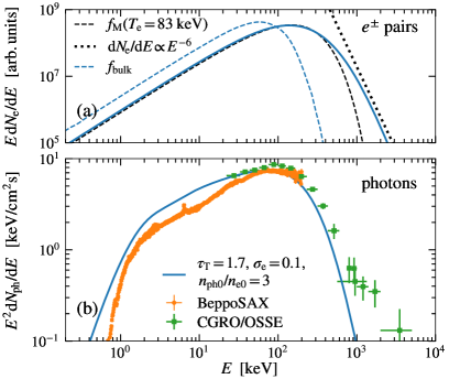
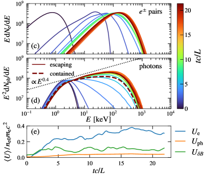
Fig. 1 demonstrates the approach to a statistically steady turbulent state in our fiducial PIC simulation. The charged particles and photons are energized by the turbulent cascade, reaching a quasi-steady state in roughly three light-crossing times $L/c$ . Unless stated otherwise, the various statistical averages reported below represent the mean values over the quasi-steady state starting at $tc/L\approx 3$ and extending until the end of the simulation. The fully developed turbulent state exhibits random “flaring” activity associated with the buildup and release of magnetic energy (Fig. 1(c)). The system is radiation-dominated and strongly magnetized in the sense that both the box-averaged photon energy density $\langle U_{\rm ph}\rangle=n_{\rm ph0}\overline{E}_{\rm ph}$ and the fluctuating magnetic energy density $\langle U_{\delta B}\rangle=\langle\delta B^{2}\rangle/8\pi$ exceed the average kinetic energy density $\langle U_{\rm e}\rangle=n_{\rm e0}\overline{E}_{\rm e}$ of pairs.

Figure 1: Time evolution of the electron-positron (a) and escaping photon (b) energy spectrum, and the evolution of the box-averaged plasma, radiation, and magnetic energy density (c). Different colors in panels (a) and (b) represent the simulation time. Also shown is the spectrum of photons contained in the domain at the end of the simulation (dashed red curve in panel (b)).

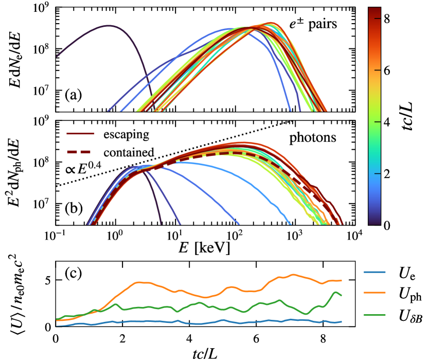
Consistent with observations [7], the escaping radiation spectrum exhibits in the statistically steady state a photon index close to $\Gamma\approx 1.6$ between the photon injection energy of roughly 1 keV and the peak near 100 keV (corresponding to $E^{2}{\rm d}N_{\rm ph}/{\rm d}E\propto E^{-\Gamma+2}\sim E^{0.4}$ in Fig. 1(b)). For our simulation parameters with $\overline{E}_{0}/m_{\rm e}c^{2}\approx 2.7\times 10^{-3}$, $\delta B/B_{0}\approx 1$ and $l_{\rm esc}/l_{0}\approx 1.3$ , Eq. (1) gives $A\approx 12$, in reasonable agreement with the typical value $A\approx 9$ measured in the simulation. The compactness $\ell\approx 19$ [45], which is comparable to the typical value $\ell\sim 50$ inferred for the hard state of Cyg X-1 [6]. The simulated compactness is too low for a self-consistent balance between pair creation and annihilation [45]. Thus, a pair plasma composition is assumed here for computational convenience only. That our model does not include heavier ions is an aspect worth considering when comparing our results to magnetohydrodynamic (MHD) simulations.

The pairs develop over time a nonthermal spectrum (Fig. 1(a)) with mean kinetic energy per particle $\overline{E}_{\rm e}/m_{\rm e}c^{2}\approx 0.5$. The nonthermal tail ($E_{\rm e}\gtrsim 600$ keV) contains about 30% of the kinetic energy. The effective temperature is raised by particles from the nonthermal tail to $\Theta_{\rm eff}\approx 0.6$. A thermal plasma with the same $\overline{E}_{\rm e}$ as measured in our simulation would have a proper temperature $T_{\rm e}/m_{\rm e}c^{2}\approx 0.3$. For reference, Eq. (2) predicts $\Theta_{\rm eff}\approx 0.2$ for our measured $\overline{E}_{\rm esc}/\,\overline{E}_{\rm ph}\approx 1.4$ and $f_{\rm KN}\approx 0.5$ . For the cooling time scale we find $t_{\rm IC}/t_{0}\approx 0.2$. Thus, the pairs pass their energy to the photons on a time scale shorter than the turbulent cascade time.

Emission mechanism.—The Comptonization of photons can occur through internal or bulk motions. In the fast cooling regime ($t_{\rm IC}<t_{0}$), a fraction $f_{\rm bulk}$ of the turbulence power is passed to the photons via bulk Comptonization before the cascade reaches the plasma microscales, leading to radiative damping of the turbulent flow [58, 59, 51]. This is demonstrated in Fig. 2, which shows the turbulence energy spectra $E(k_{\perp})$, defined as the sum of magnetic, electric, and bulk kinetic energy density spectra . The spectrum $E(k_{\perp})$ from our run with $\tau_{\rm T}=1.7$ is compared against the result obtained from a simulation with $\tau_{\rm T}=0.2$ but otherwise identical parameters. The spectra extend from the injection scale ($k_{\perp}d_{\rm e0}\sim 0.01$) into the kinetic range ($k_{\perp}d_{\rm e0}\gtrsim 1$), where the cascaded energy converts into plasma internal motions. Over the MHD range ($k_{\perp}d_{\rm e0}\ll 1$) the turbulence spectrum for $\tau_{\rm T}=0.2$ exhibits a slope consistent with a classical cascade where $E(k_{\perp})\propto k_{\perp}^{-5/3}$ [61, 62], while for $\tau_{\rm T}=1.7$ the radiative damping becomes strong enough to steepen the spectrum (Fig. 2(a)). This can be considered an example for how radiative effects render the turbulence spectra non-universal.

Figure 2: 1D power spectra $E(k_{\perp})$ of the turbulence energy as a function of the wavenumber $k_{\perp}$ perpendicular to $\mathbf{B}_{0}$ for $\tau_{\rm T}=1.7$ and $\tau_{\rm T}=0.2$ (a). Panel (b) shows the ratio of the turbulent spectra from the two simulations.

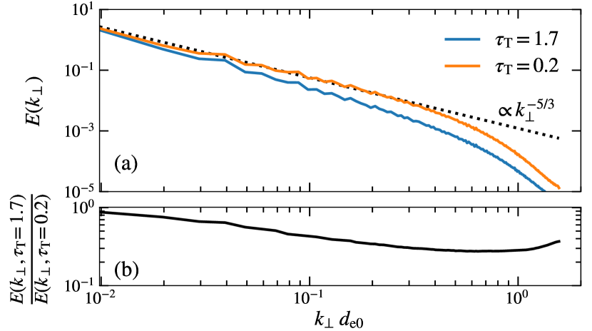
The steepening of the turbulence spectrum in our fiducial simulation with $\tau_{\rm T}=1.7$ is related to the power lost via bulk Comptonization as follows. In the MHD range, it may be assumed that $\Pi_{k_{\perp}}\sim{\mathcal{F}}_{0}-{\mathcal{D}}^{\rm rad}_{k_{\perp}}$, where $\Pi_{k_{\perp}}$ is the turbulent energy flux to perpendicular wavenumbers larger than $k_{\perp}$, ${\mathcal{F}}_{0}$ is the external driving confined to the wavenumber $k_{0}\ll k_{\perp}$, and ${\mathcal{D}}^{\rm rad}_{k_{\perp}}$ is the radiative dissipation rate between $k_{0}$ and $k_{\perp}$. Since a fraction $f_{\rm bulk}$ of the cascade power is lost to radiation, we have ${\mathcal{D}}^{\rm rad}_{k_{\max}}\sim f_{\rm bulk}{\mathcal{F}}_{0}$, and so $\Pi_{k_{\perp}}/\Pi_{0}\sim 1-f_{\rm bulk}{\mathcal{D}}^{\rm rad}_{k_{\perp}}/{\mathcal{D}}^{\rm rad}_{k_{\max}}$, where $\Pi_{0}\sim{\mathcal{F}}_{0}$ is the energy flux in the absence of damping. The flux can be approximated as $\Pi_{k_{\perp}}\propto k_{\perp}^{2+\alpha}E(k_{\perp})^{1+\alpha}$, with $\alpha=1/2$ for the Goldreich-Sridhar turbulence model [61, 62]. There follows the estimate

$$E(k_{\perp})/E_{0}(k_{\perp})\sim\left(1-f_{\rm bulk}{\mathcal{D}}^{\rm rad}_{k_{\perp}}/{\mathcal{D}}^{\rm rad}_{k_{\max}}\right)^{\frac{1}{1+\alpha}},$$ (3)

where $E_{0}(k_{\perp})$ is the spectrum in the absence of significant damping. At the tail of the MHD range ($k_{\perp}d_{\rm e0}\sim 0.5$), we have $f_{\rm bulk}\sim 1-(E(k_{\perp})/E_{0}(k_{\perp}))^{1+\alpha}$, which can be taken as a proxy for measuring $f_{\rm bulk}$. We substitute for $E_{0}(k_{\perp})$ the spectrum obtained for $\tau_{\rm T}=0.2$ and estimate from Fig. 2(b) that $E(k_{\perp})/E_{0}(k_{\perp})\approx 0.3$ near $k_{\perp}d_{\rm e0}\approx 0.5$ , indicating that roughly $f_{\rm bulk}\approx 80$% (using $\alpha=1/2$) of the total cascade power is passed to the photons via bulk Comptonization. The turbulent flow is dominated by motions transverse to the magnetic field [64], which renders the emission anisotropic. The intensity of Comptonized radiation escaping parallel to $\mathbf{B}_{0}$ is about 3 times lower than the intensity emitted perpendicular to the mean magnetic field. Note that efficient bulk Comptonization is generally expected when the particles cool quickly ($t_{\rm IC}<t_{0}$). Guided by our simulation, we can give a simple estimate of $f_{\rm bulk}$ for $t_{\rm IC}<t_{0}$ as $f_{\rm bulk}\sim 1-t_{\rm IC}/t_{0}\sim 1-(\overline{E}_{\rm e}/m_{\rm e}c^{2})[\sigma_{\rm e}(\delta B/B_{0})^{2}]^{-1}$, which connects bulk Comptonization to the high-$\sigma_{\rm e}$ regime.

Figure 3: Spatial structure of $\Theta_{\rm eff}-\Theta_{\rm bulk}$ (a), $U_{\rm ph}$ (b), and $\left|\mathbf{J}\right|$ (c), where $\Theta_{\rm eff}$ is the effective plasma temperature, $\Theta_{\rm bulk}$ is the “temperature” of turbulent bulk motions, $U_{\rm ph}$ is the photon energy density, and $\left|\mathbf{J}\right|$ is the magnitude of the plasma electric current.

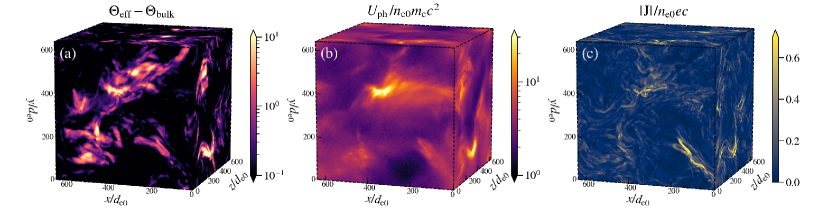
Efficient bulk Comptonization implies that the plasma is essentially cold and its effective temperature is close to the “temperature” of turbulent bulk motions $\Theta_{\rm bulk}\equiv u_{\rm bulk}^{2}/3$ [8], where $u_{\rm bulk}^{2}=\beta^{2}_{\rm bulk}/(1-\beta^{2}_{\rm bulk})$ is the squared bulk four-velocity in units of $c^{2}$. In the simulation with $\tau_{\rm T}=1.7$ we find on average $\Theta_{\rm bulk}/\Theta_{\rm eff}\approx$ 50%. In Fig. 3 we visualize the local difference $\Theta_{\rm eff}-\Theta_{\rm bulk}$ at time $tc/L=6$ in our fiducial simulation. For reference, we also show the structure of the photon energy density and the magnitude of the plasma electric current. Over much of the volume the plasma is indeed cold, in the sense that at most locations the difference $\Theta_{\rm eff}-\Theta_{\rm bulk}$ is very moderate. In a small fraction of the volume, typically near electric current sheets, the turbulent energy is intermittently released into internal motions, giving rise to “hot spots” with $\Theta_{\rm eff}-\Theta_{\rm bulk}\gtrsim 1$. The hot spot formation requires a rapid form of energy release in order to outpace the fast cooling. One promising candidate is magnetic reconnection [45], which is known to promote particle energization magnetically dominated MHD [65, 66, 67, 68, 69, 70, 71, 72, 73, 74] and kinetic [31, 37, 75, 76, 77] turbulent plasmas.

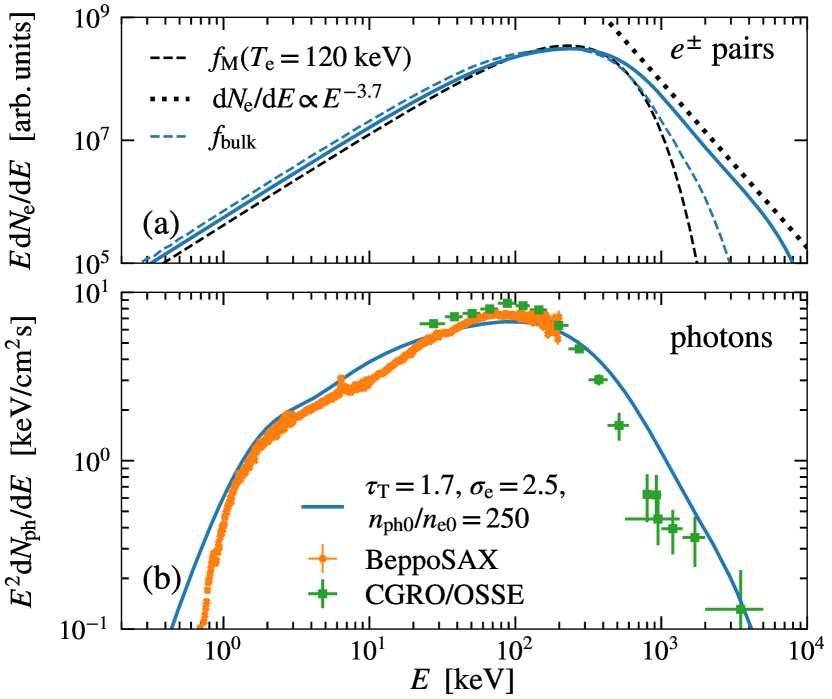
Observational implications.—Fig. 4 shows the spectra from our fiducial PIC simulation, time-averaged over steady state, together with observations of Cyg X-1 in the hard state. The obtained emission spectrum closely resembles the observations. Differences between our simulation and observations are seen below 1 keV, where the observed spectrum is attenuated by absorption, between 10 keV and the peak, and around 1 MeV. We do not include the additional radiation component that is Compton-reflected from the disk [4], which affects the spectrum in the range between roughly 10 keV and the peak. Regarding the MeV tail, we note that the inclusion of synchrotron cooling [7] and pair creation [78, 79] could soften the tail. Simulations with electron-ion compositions, pair creation and annihilation, and/or synchrotron emission can further constrain the physical conditions required to reproduce the observed MeV tail.

The strongly magnetized regime ($\sigma_{\rm e}\gtrsim 1$) explored here corresponds to a radiatively compact corona ($\ell\gtrsim 10$) located roughly within 10 gravitational radii from the black hole [45]. A natural feature of our model is the formation of a nonthermal electron tail (Fig. 4(a)), which shapes the MeV emission. The distribution due to bulk motions alone (dashed blue curve in Fig. 4(a)) is significantly less nonthermal than the full distribution (solid blue curve), which implies that the nonthermal tail is mostly contributed by internal motions. We ran an additional simulation at $\sigma_{\rm e}=0.1$ and found in comparison to our fiducial run a weaker nonthermal electron tail [45]. The results may also depend on the type of turbulence driving (e.g., the low-amplitude regime with $\delta B\ll B_{0}$ is less favorable for the production of nonthermal particles [45, 30, 32]).

Figure 4: Energy spectra of electron-positron pairs (a) and of the escaping radiation (b), overplotted with observations of the hard state in Cyg X-1 from BeppoSAX [80, 81] and CGRO/OSSE [82]. The emission spectra are normalized with respect to OSSE. Dashed blue curve in panel (a) shows the energy distribution due to bulk motions alone. The dashed black curve shows a Maxwellian distribution fitted below 400 keV.

Conclusions.—We performed the first PIC simulations of plasma turbulence that self-consistently follow the evolution of radiation via Compton scattering. Our simulations focus on the conditions expected in magnetized coronae of accreting black holes [4, 6], which have moderate optical depths and experience fast radiative cooling. Similar conditions can also arise in jets of gamma-ray bursts [58, 83, 59, 84, 85, 51]. We obtain a spectrum of escaping X-rays similar to the observed hard-state spectrum of Cyg X-1, thus demonstrating that kinetic turbulence is a viable mechanism for the energization of electrons in black-hole coronae.

While the Compton scattering between the turbulent kinetic plasma and the radiation is treated self-consistently, we note that our present setup is still subject to a number of limitations. We do not model the emission of soft photons, pair creation, annihilation, or the global structure of the extended corona and the accretion disk. Instead, we adopt a local 3D periodic box approximation with a fixed average pair number density and with soft photon injection matching photon escape to sustain a fixed photon-to-electron ratio. A complete understanding of the X-ray emission from black-hole coronae may require a global kinetic model with detailed radiative transfer, which is presently lacking. Existing global models based on MHD simulations (e.g., [9, 10, 11]) suggest that the properties of the observed X-rays depend not only on the mechanism of local energy release into radiation, but also on the geometric shape and multiphase structure of the corona.

In our local model, the emission is produced via Comptonization in a plasma energized by large-amplitude ($\delta B\sim B_{0}$) Alfvénic turbulence. For a strongly magnetized plasma, we find that most of the turbulence power is directly passed to the photons through bulk Comptonization. The rest is channeled into nonthermal particles at localized hot spots. For computational convenience, our simulations employ a pair plasma composition. The nature of turbulent Comptonization in electron-ion plasmas could differ from that in pair plasmas [45]. An important parameter is the fraction of turbulence power channeled into ion heating, which needs to be investigated with dedicated simulations. We also show that turbulent Comptonization manifests itself through non-universal turbulence spectra. As such, our simulations give a glimpse into a new regime of kinetic turbulence in radiative plasmas of moderate optical depth.

Supplemental Material for “Radiative Particle-in-Cell Simulations of Turbulent Comptonization in
Magnetized Black-Hole Coronae”

I Radiative compactness and electron-positron pair balance

The particle composition of black-hole coronae may be electron-ion or pair dominated, depending on the radiative compactness $\ell$ and on the energy distribution of the Comptonizing electrons [54, 78, 79, 86, 6, 23]. In particular, pair dominated states are associated with radiatively compact sources ($\ell\gg 1$). In a local cubic slab of linear size $L$ the radiative compactness may be defined as $\ell=P_{\rm diss}\sigma_{\rm T}/Lm_{\rm e}c^{3}$ (e.g., [86]), where $P_{\rm diss}$ is the dissipated power transferred to the radiation. For our simulation setup we estimate $P_{\rm diss}\simeq L^{3}\delta B^{2}/4\pi t_{0}$. Using $L=2l_{\rm esc}$ we obtain

$$\ell\simeq 4\tau_{\rm T}\sigma_{\rm e}\!\left(\delta B/B_{0}\right)^{3}\!\left(v_{\rm A}/c\right)\!\left(l_{\rm esc}/l_{0}\right).$$ (1)

This shows that a high magnetization ($\sigma_{\rm e}\gtrsim 1$) translates into a large radiative compactness in our model, consistent with previous arguments in support of a magnetically dominated corona [48]. In our fiducial simulation we obtain $\ell\approx 19$, which is comparable to the typical value $\ell\sim 50$ inferred for Cyg X-1 [6]. It is also consistent with the broader range $\ell\sim 1-100$ representative of black-hole coronae in active galactic nuclei [101]. The regime $\ell\lesssim 1$ can be identified with $\sigma_{\rm e}\ll 1$. Here, the electrons are only mildly nonthermal, their cooling is slow, and the emission mechanism is essentially thermal Compotonization (see Sec. II). Using Eq. (1) from the main Letter, we can alternatively express $\ell\sim 4\bigl{(}n_{\rm ph0}/n_{\rm e0}\bigr{)}\bigl{(}\overline{E}_{\rm esc}/m_{\rm e}c^{2}\bigr{)}\bigl{[}\tau_{\rm T}/(\tau_{\rm T}+1)\bigr{]}$, which shows that $\ell$ scales in proportion to $n_{\rm ph0}/n_{\rm e0}$. In global accretion models, one can also estimate $\ell\sim 4\pi(m_{\rm p}/m_{\rm e})\tilde{R}^{-1}\tilde{L}$ [6], where $m_{\rm p}$ is the proton mass, $\tilde{L}$ is the luminosity in units of the Eddington luminosity, and $\tilde{R}$ is a characteristic size of the source in units of the gravitational radius. A luminous black hole accreting at a few per cent of the Eddington limit has roughly $\ell\gtrsim 10$ when $\tilde{R}\lesssim 10$. Thus, the high magnetization regime ($\sigma_{\rm e}\gtrsim 1$) of our local model corresponds to a radiatively compact corona located roughly within 10 gravitational radii or so from the black hole.

It is worth estimating how close (or far) is our fiducial PIC simulation from a state of pair balance, where pair creation is balanced by annihilation. A simple but direct estimate can be given based on a set of analytic approximations [79, 16] for the time scales of pair creation, $t_{\gamma\gamma}=n_{\rm e^{+}}/\dot{n}_{\gamma\gamma}$, and annihilation, $t_{\rm ann}=n_{\rm e^{+}}/\dot{n}_{\rm ann}$. In our notation, these can be expressed as:

$$t_{\gamma\gamma}/t_{\rm esc} \sim\frac{n_{\rm e0}^{2}/n_{\rm ph0}^{2}}{2\eta f_{1}^{2}\,\tau_{\rm T}(1+\tau_{\rm T})}, t_{\rm ann}/t_{\rm esc} \sim\frac{16}{3\tau_{\rm T}(1+\tau_{\rm T})},$$ (2)

where $f_{1}$ is the fraction of photons with energies $E_{\rm ph}\geq m_{\rm e}c^{2}$, $\eta\sim 0.1$ [79], and $t_{\rm esc}$ is the photon escape time. This gives $t_{\gamma\gamma}/t_{\rm esc}\sim 30$ and $t_{\rm ann}/t_{\rm esc}\sim 1$ for our measured $f_{1}\approx 7.2\times 10^{-4}$. Taken at face value, the estimated rate of pair production is too slow to maintain an optical depth $\tau_{\rm T}\sim 1$. The electron-positron particle composition is chosen here mainly for simplicity, given that an equivalent simulation with heavier ions is computationally infeasible at present. On the other hand, it should be also noted that the time scale of pair creation in Eq. (2) is only a crude estimate, obtained for an isotropic and homogeneous radiation field. Moreover, $t_{\gamma\gamma}$ is very sensitive to the number of photons in the MeV tail, such that even moderate changes in the input parameters can lead to large differences in the pair creation rate. According to the crude estimate from above, a pair balanced state ($t_{\gamma\gamma}\sim t_{\rm ann}$) might be obtained in our model for a compactness of the order of 100 or so. Radiative PIC simulations with self-consistent pair creation and annihilation are required to accurately constrain the parameters of pair-balanced states for the turbulent Comptonization model.

II Plasma-dominated regime with slow radiative cooling ($\sigma_{\rm e}\ll 1$)

Our Letter focuses on the application of turbulent cascades to sources with fast radiative cooling of electrons, as appropriate for magnetized coronae of accreting black holes [48, 6]. This can be contrasted with the slow cooling regime, which corresponds to $\sigma_{\rm e}\ll 1$ in our model. In Fig. 1 we show for reference results from a simulation with $\sigma_{\rm e}=0.1$. In order to achieve an amplification factor $A\sim 10$ at the reduced value of $\sigma_{\rm e}$ we set $n_{\rm ph0}/n_{\rm e0}=3$ (according to Eq. (1) from the main Letter). Other simulation parameters match those reported in the main Letter.

Figure 1: Results from a PIC simulation performed in the low-$\sigma_{\rm e}$ regime with slow radiative cooling.

As shown in Fig. 1(e), the system evolves toward a state where the particle kinetic energy density ($U_{\rm e}$) dominates over the magnetic ($U_{\delta B}$) and radiation ($U_{\rm ph}$) energy density. In the quasi-steady state (starting around $\approx 7L/c$), we measure $A\approx 7$ and $\ell\approx 0.3$, which is inconsistent with the typical range $\ell\sim 1-100$ inferred from observations of accreting black holes. As expected, the turbulent cascade is in the slow cooling regime with $t_{\rm IC}/t_{0}\approx 3$. Moreover, the electron energy distribution (Fig. 1(a)) features only a mild nonthermal tail (at $E_{\rm e}\gtrsim$ 600 keV), which contains less than 10% of the kinetic energy. As a result, the escaping photon spectrum shows no significant emission in the MeV range (Fig. 1(b)).

III Turbulent Comptonization in electron-ion plasmas

All simulations presented here employ for simplicity an electron-positron pair particle composition. However, the composition of the coronal plasma may be dominated by ions and electrons rather than pairs (see Sec. I for a discussion). If the particle composition is dominated by electrons and heavier ions (i.e., protons) an additional parameter enters the problem: the fraction $q_{\rm i}$ of turbulence power channeled into ion heating. The parameter $q_{\rm i}$ needs to be determined from kinetic models and simulations; it has been extensively studied in nonradiative simulations (e.g., [28, 98]) and in one set of simulations with inverse-Compton cooling of relativistically hot electrons [38]. The ion heating fraction in the regime relevant to this work ($\tau_{\rm T}\sim 1$, fast Compton cooling, and mildly relativistic electrons) has not been investigated. Our scalings, obtained for a pair plasma, can be easily adapted for the electron-ion case. We find

$$A \sim 1+(1-q_{\rm i})\sigma_{\rm e}(\tau_{\rm T}+1)\left(\!\frac{\overline{E}_{0}}{m_{\rm e}c^{2}}\!\right)^{\!\!\!-1}\!\!\left(\!\frac{n_{\rm e0}}{n_{\rm ph0}}\!\right)\left(\!\frac{v_{\rm A}}{c}\!\right)\left(\!\frac{\delta B}{B_{0}}\!\right)^{\!\!3}\!\left(\!\frac{l_{\rm esc}}{l_{0}}\!\right),$$ (3)

$$\ell \sim 4\tau_{\rm T}(1-q_{\rm i})\sigma_{\rm e}\left(\delta B/B_{0}\right)^{3}\left(v_{\rm A}/c\right)\left(l_{\rm esc}/l_{0}\right),$$ (4)

$$t_{\rm IC}/t_{0} \sim(\overline{E}_{\rm e}/m_{\rm e}c^{2})\left[(1-q_{\rm i})\sigma_{\rm e}(\delta B/B_{0})^{2}\right]^{-1},$$ (5)

where the Alfvén speed $v_{\rm A}=c[\sigma_{\rm i}/(1+\sigma_{\rm i})]^{1/2}$ is now determined by the ion magnetization $\sigma_{\rm i}$. For subrelativistic ions $\sigma_{\rm i}\simeq B_{0}^{2}/4\pi n_{\rm i0}m_{\rm i}c^{2}\simeq\sigma_{\rm e}(n_{\rm e0}/n_{\rm i0})(m_{\rm e}/m_{\rm i})\simeq\sigma_{\rm e}m_{\rm e}/m_{\rm i}$.

A model based on an electron-ion composition presents a set of open questions with respect to observations. Unless almost all energy goes into ion heating ($1-q_{\rm i}\ll 1$), we require $\sigma_{\rm i}\sim\sigma_{\rm e}m_{\rm e}/m_{\rm i}\ll 1$ for typical values of the compactness $\ell\sim$ a few 10. A high radiative compactness implies also fast cooling ($t_{\rm IC}<t_{0}$). It is then expected that the turbulence is subject to radiative damping and a significant fraction of its power is lost before the energy cascades to the plasma microscales, which is reminiscent of the bulk Comptonization scenario. However, it is not obvious how the electrons can be maintained at energies of about 100 keV if their bulk motions with $\delta v\sim v_{\rm A}$ are nonrelativistic (since $\sigma_{\rm i}\ll 1$) and only a small amount of the cascade power arrives at kinetic scales, where the heating usually occurs. The issue can be, in principle, avoided if one postulates a rapid form of electron energization that bypasses the turbulent cascade and draws energy from all scales of the turbulent flow. Another possibility is to assume that the large-scale turbulent motions are not constrained by $v_{\rm A}$ (i.e., that the motions are super-Alfvénic). Finally, mildly relativistic bulk motions and reasonable values of the compactness can be obtained if $\sigma_{\rm i}\sim\sigma_{\rm e}m_{\rm e}/m_{\rm i}\sim 1$ and $10^{-3}\lesssim 1-q_{\rm i}\lesssim 10^{-2}$.

In conclusion, the nature of turbulent Comptonization in electron-ion plasmas could differ from that in pair plasmas. An important parameter affecting the Comptonization is the fraction of turbulence power channeled into ion heating, which needs to be investigated with dedicated radiative PIC simulations.

IV Dependence on the system size

It is worth commenting on how the limited scale separation in our fiducial simulation ($L=2l_{\rm esc}=640d_{\rm e0}$) might affect the results. The observed emission is essentially determined by the electron energy distribution and by the optical depth, which sets the average number of scatterings experienced by a photon before escape. The effective electron temperature (Eq. (2) in the main Letter), which controls the position of the Comptonized peak, has no explicit dependence on system size, although we cannot rule out a moderate implicit dependence. This leaves in question the shape of the electron distribution, in particular its nonthermal tail, which controls the gamma-ray emission.

Particles injected into the nonthermal tail in high-$\sigma_{\rm e}$ kinetic turbulence are rapidly accelerated by the nonideal electric fields up to $\gamma\sim$ a few $\sigma_{\rm e}$ [30], and not much beyond that if subsequent acceleration is slow compared to the cooling time scale [39, 100]. Fast acceleration is, however, still possible provided that particles experience relatively coherent large-scale fields over their acceleration history. Such fields can be, for instance, present in large-scale turbulent reconnection layers (e.g., [66, 68, 69, 76, 104, 77]), where particles on both sides of the reconnecting sheet sample an ideal upstream electric field. If electrons in black-hole coronae experience fast acceleration across a broad range of scales, their maximum Lorentz factor is higher than predicted in our fiducial PIC simulation, and the coronal gamma-ray emission extends to higher energies.

V Choice of seed photon distribution

The choice of the typical seed photon energy, $\overline{E}_{0}$, is for a given source constrained by observations. It can be roughly identified with the low-energy range of the Comptonized spectrum, which is near 1 keV for Cyg X-1. What remains to be specified is the shape of the seed photon distribution. Here, we employ a Planck spectrum with temperature $T_{0}/m_{\rm e}c^{2}=10^{-3}$. This is consistent with the common view that the seed photons originate from optically thick and colder regions of the accretion flow, where the plasma and radiation are near thermal equilibrium [4], although seed photons may be additionally provided by synchrotron emission [7]. The energy budget of a turbulent cascade in a plasma of moderate optical depth is weakly affected by the choice of $T_{0}$, as long as $\overline{E}_{0}\ll\overline{E}_{\rm e}$. This is because the escaping photons are upscattered to energies $\overline{E}_{\rm esc}\gg\overline{E}_{0}$, and so essentially only the energy of the escaping photons enters the energy balance between the turbulent driving and radiative cooling.

VI Choice of the photon to pair density ratio

The mean density ratio of photons to electrons and positrons, $n_{\rm ph0}/n_{\rm e0}$, is an important parameter of our present model. Reasonable values for $n_{\rm ph0}/n_{\rm e0}$ can be inferred from Eq. (1) of the main Letter, which relates the amplification factor $A$ to the main parameters of our model. In particular, the terms in Eq. (1) show that $n_{\rm ph0}/n_{\rm e0}$ scales in proportion to $\sigma_{\rm e}v_{\rm A}/c$ for a fixed value of $A$. For a typical hard state in X-ray binaries with $A\sim 10$ we require $n_{\rm ph0}/n_{\rm e0}\gtrsim 100$ when the corona is strongly magnetized ($\sigma_{\rm e}\gtrsim 1$). The effect of the density ratio on the energy spectra can be also seen in Fig. 2, which presents a set of numerical convergence checks performed at two different values of $n_{\rm ph0}/n_{\rm e0}$. Physically, the photon to electron density ratio in the corona is controlled by the global state of accretion and/or by the local balance between pair creation, annihilation, photon emission and absorption.

VII Role of the turbulence driving

The structure of coronal turbulence in luminous black-hole accretion flows is presently the subject of ongoing investigations. A firm understanding will likely require extreme resolution global 3D MHD simulations, of similar type as recently presented for low-luminosity sources [103], where the nature of high-energy emission is different (e.g., [97]). In our local model, we drive the turbulence by imposing a large-scale time-varying external current [46]. This type of driving excites predominantly, though not exclusively, Alfvénic perturbations (for discussions of different types of turbulence driving see Refs. [93, 98, 102]). For strong turbulence an appropriate choice of the amplitude is then such that $\delta B\sim B_{0}$. Strong magnetic perturbations are implicitly assumed throughout this work, although the assumption can be relaxed if necessary. Perturbations with $\delta B\sim B_{0}$ could originate, for instance, from the large-scale twisting and bending of coronal field lines, anchored in the turbulent accretion disk and in the black-hole magnetosphere. In contrast, low-amplitude magnetic fluctuations ($\delta B\ll B_{0}$) would result in a more ordered and smooth magnetic field line configuration in the corona. Such perturbations could be driven by small-scale ($l_{0}\ll l_{\rm esc}$) waves and instabilities in the accreting flow. The low-amplitude regime of wave turbulence faces a similar challenge as the low-$\sigma_{\rm e}$ scenario (see Sec. II). Namely, the expected electron distributions are nearly thermal [32] and cannot account for the MeV tail of the observed emission [7]. A model based on low-amplitude turbulent driving of the corona would have to consistently explain where the missing MeV tail of the emission comes from and how it is produced, if not in the corona.

VIII Comptonization via turbulence and/or reconnection

It is worth commenting on how the scenario put forward in the present work differs from earlier PIC studies of Comptonization via bulk motions driven by 2D magnetic reconnection [17, 18, 20]. Reconnection in 2D current sheets proceeds through the formation of non-turbulent plasmoid chains; photons are then Comptonized by the bulk plasmoid motions. In contrast, in the present 3D simulations bulk Comptonization is mediated by turbulent motions spanning a broad range of scales. It should be noted that turbulence and reconnection in real 3D systems are intrinsically connected (e.g., [70, 96, 99]). Moreover, turbulence in magnetized plasmas is known to form current sheets (e.g., [87, 65, 88, 89, 67, 91, 92, 70, 94]), which are also observed in our present simulations (Fig. 3 of the main Letter). To understand the details of how the energy transfer occurs through the reconnecting layers in 3D turbulent flows is still an open question and requires further investigation.

IX Additional numerical details

The Compton scattering between macroparticles in a given collision cell is calculated using a Monte Carlo approach [43, 44]. The method is based on the selection of a random sample of electron-photon (or positron-photon) couples that constitute a list of “candidates” for the Compton scattering in a given collision cell and at a given time step. The computational particles from the randomly generated list are then scattered with a given probability, which is proportional to the scattering cross section and inversely proportional to the size of the random sample. In black-hole coronae and other radiatively compact sources [6], the mean number density of physical photons to electron-positron pairs $n_{\rm ph0}/n_{\rm e0}\gg 1$, implying that the frequency of binary collisions experienced by an electron (or positron) is greatly enhanced compared to a photon, and relatively large samples of electron-photon (or positron-photon) couples are needed for the scattering to be properly captured. To this end, we employ a random sampling where each electron (or positron) is paired with at least $i\geq 1$ different photons, with $i$ large enough to obtain a good statistical sample for a given collision cell. In particular, we determine $i$ at every time step and for each cell based on the condition that the maximum probability for an electron to scatter with a given photon from the sample is less than 10%. Typical values of $i$ in our fiducial simulation lie between a few and ten. Compared to the standard Monte Carlo sampling, where each particle is paired at most once per step, our method represents essentially a form of adaptive substepping of the elementary time step. It is also worth mentioning that, under the physical conditions explored in this work, an electron typically experiences an order-unity deflection only after several binary collisions because most scatterings occur in the Thomson regime.

We use the same average number of computational particles for photons as for the electron-positron pairs, and therefore the probability of an electron macroparticle to scatter is $p_{\rm e}=p_{\rm ph}n_{\rm ph0}/n_{\rm e0}$, where $p_{\rm ph}$ is the scattering probability for the photon. We account for the unequal collision probabilities ($p_{\rm e}>p_{\rm ph}$) using a rejection method [90]. For each couple from the sample, we draw a uniform random number $r\in[0,1)$, determine $p_{\rm e}$ and $p_{\rm ph}$, and calculate the new momenta of the electron (or positron) and photon after scattering if $p_{\rm e}>r$. The momentum of the electron is updated to the new value if $p_{\rm e}>r$, whereas the momentum of the photon is updated if $p_{\rm ph}>r$. The rejection method [90] does not conserve energy and momentum per each Monte Carlo collision, but still does so in a statistical sense. An alternative that conserves energy and momentum per collision involves splitting of particles [43, 44], followed by occasional particle merging [95]. The latter is impractical in the regime explored here, since it would require very frequent merging throughout the whole simulation.

Figure 2: Dependence of the electron-positron (a,c) and photon (b,d) energy spectra on various numerical parameters (see the main supplement text for details). All spectra are shown at around $t=2L/c$.

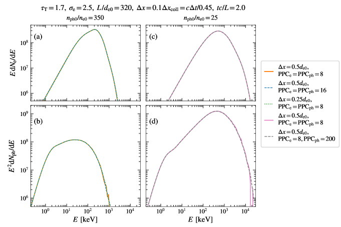
In Fig. 2 we present a set of numerical convergence checks using a computational box of size $L/d_{\rm e0}=320$, which is half the size used in the main Letter. Same as in the main Letter, we set $\tau_{\rm T}=1.7$, $\sigma_{\rm e}=2.5$, and $\Delta x=0.1\Delta x_{\rm coll}=c\Delta t/0.45$, where $\Delta x$ is the size of a PIC grid cell, $\Delta x_{\rm coll}$ is the size of a collision cell for scattering, and $\Delta t$ is the time step. In panels 2(a)-2(b) we use $n_{\rm ph0}/n_{\rm e0}=350$ and check the dependence on the number of particles per cell of the PIC grid ($\rm PPC_{\rm e}$ for pairs and $\rm PPC_{\rm ph}$ for photons), and on the spatial resolution. Our reference simulation with $\Delta x=0.5d_{\rm e0}$ and $\rm PPC_{\rm e}=\rm PPC_{\rm ph}=8$ (same as used in the main Letter) is then compared against a simulation with $\rm PPC_{\rm e}=\rm PPC_{\rm ph}=16$ and another one where $\Delta x$, $\Delta x_{\rm coll}$, and $\Delta t$ are all twice smaller ($\Delta x=0.25d_{\rm e0}$). In panels 2(c)-2(d) we use $n_{\rm ph0}/n_{\rm e0}=25$ and compare the results obtained for $\rm PPC_{\rm e}=\rm PPC_{\rm ph}=8$ against a simulation where $\rm PPC_{\rm e}=8$ but $\rm PPC_{\rm ph}=25\cdot 8=200$, such that ${\rm PPC}_{\rm ph}/{\rm PPC}_{\rm e}=n_{\rm ph0}/n_{\rm e0}$. We use here a more moderate value for $n_{\rm ph0}/n_{\rm e0}$ due to memory limitations imposed by the choice ${\rm PPC}_{\rm ph}/{\rm PPC}_{\rm e}=n_{\rm ph0}/n_{\rm e0}\gg 1$. When the latter condition is satisfied, the computational electrons and photons are scattered with equal probabilities ($p_{\rm e}=p_{\rm ph}$) because each macro-photon represents the same number of physical particles as a macro-electron. The energy and momentum in the simulation with ${\rm PPC}_{\rm ph}/{\rm PPC}_{\rm e}=n_{\rm ph0}/n_{\rm e0}$ are thus conserved in each Monte Carlo collision, which can be compared against the results obtained using the rejection method with $\rm PPC_{\rm e}=\rm PPC_{\rm ph}$, where the conservation only holds in a statistical sense. We find that all electron-positron and photon spectra shown in panels 2(a)-2(b) and 2(c)-2(d) are in excellent agreement and conclude that for our typical choice of numerical parameters the results are well converged.