Distributed Optimization Methods for Multi-Robot Systems: Part I — A Tutorial

Abstract

Distributed optimization provides a framework for deriving distributed algorithms for a variety of multi-robot problems. This tutorial constitutes the first part of a two-part series on distributed optimization applied to multi-robot problems, which seeks to advance the application of distributed optimization in robotics. In this tutorial, we demonstrate that many canonical multi-robot problems can be cast within the distributed optimization framework, such as multi-robot simultaneous localization and planning (SLAM), multi-robot target tracking, and multi-robot task assignment problems. We identify three broad categories of distributed optimization algorithms: distributed first-order methods, distributed sequential convex programming, and the alternating direction method of multipliers (ADMM). We describe the basic structure of each category and provide representative algorithms within each category. We then work through a simulation case study of multiple drones collaboratively tracking a ground vehicle. We compare solutions to this problem using a number of different distributed optimization algorithms. In addition, we implement a distributed optimization algorithm in hardware on a network of Rasberry Pis communicating with XBee modules to illustrate robustness to the challenges of real-world communication networks.

I Introduction

Distributed optimization is the problem of minimizing a joint objective function subject to constraints using an algorithm implemented on a network of communicating computation nodes. In this tutorial, we specifically consider the computation nodes as robots and the network as a typical multi-robot mesh network. While distributed optimization has been a longstanding topic of research in the optimization community (e.g., [1, 2]), its usage in multi-robot systems is limited to only a handful of examples. However, we note that many problems in multi-robot coordination and collaboration can be formulated and solved within the framework of distributed optimization, including cooperative estimation [3], distributed SLAM, multi-agent learning [4], and collaborative motion planning [5].

This tutorial constitutes the first part of a two-part series on distributed optimization methods for multi-robot systems. While this tutorial focuses on the amenability of a broad class of multi-robot problems to distributed optimization, the second part of the series provides a survey of existing distributed optimization methods, with an emphasis on their applications to multi-robot problems, and highlights open research problems in distributed optimization for multi-robot systems. In this tutorial, we introduce the framework of distributed optimization, noting the important components of this framework. In distributed optimization, several robots (agents/computational nodes) collectively optimize a shared decision variable, where each agent has knowledge of only its local objective and constraint function, without knowing the objective and constraint functions of other agents. The joint objective function is typically taken as the sum over all the robots of their local objectives, and the constraints are the union of their local constraints. As a result, each agent only has partial knowledge of the joint optimization problem and cannot solve the joint problem individually. We assume that each robot can communicate with its immediate one-hop neighbors over a robot-to-robot communication network, which is representative of the communication network present in many robotics problems. We do not include the many existing algorithms that require multi-hop communication or require a hub-spoke network topology, where all agents communicate to a central hub, as these network requirements are incompatible with the typical multi-robot network model.

Although the joint problem can be solved through centralized optimization, centralized optimization techniques require significant computation and communication resources due to the need for data aggregation at a central hub, making this approach less appealing in a multi-robot setting, especially with a large number of robots. Distributed optimization algorithms enable each robot to solve for an optimal solution of the joint optimization problem locally, in parallel, while communicating with its one-hop neighbors over a communication network. In general, these algorithms are iterative, with each robot sharing its intermediate decision variables or problem gradients with its neighbors at each iteration. However, robots do not share information about their local objective and constraint functions or their problem data, such as local measurements, leading to an inherent privacy property for these algorithms. The decision variables of all the robots converge to a common solution of the optimization problem as the algorithm proceeds. In convex problems, the solution computed by each robot corresponds to a globally optimal solution; however, in non-convex problems, the iterates of each robot generally converge to a locally optimal solution. This tutorial is directed towards robotics practitioners who want to derive the benefits of distributed optimization in robotics, in addition to robotics researchers interested in research encompassing distributed optimization and multi-robot systems.

We demonstrate in this tutorial that a number of major multi-robot problems can be formulated as distributed optimization problems, such as multi-robot simultaneous localization and mapping (SLAM), multi-robot target tracking, multi-robot task assignment, collaborative trajectory planning, and multi-robot learning. We describe the general strategies useful in reformulating robotics problems into a form amenable to distributed optimization algorithms. We note that optimization-based approaches often provide flexibility in solving many robotics problems. For example, multi-robot target tracking problems are typically solved via filtering or smoothing approaches, posing certain challenges such as cross-correlation of local measurements [6]. In contrast, formulating multi-robot target tracking problems as optimization problems eliminates these drawbacks.

We categorize distributed optimization algorithms into the following classes: distributed first-order methods, distributed sequential convex programming, and the alternating direction method of multipliers (ADMM). We describe the defining mathematical technique of each category and provide representative algorithms for each category. Lastly, we provide a case study on multi-drone ground vehicle tracking, where we demonstrate the application of distributed optimization to the target tracking problem in simulation, and in addition, implement a distributed optimization algorithm on hardware using the XBee DigiMesh 2.4 network modules for communication.

I-A Contributions

This tutorial paper has three primary objectives:

1. Demonstrate the formulation of many canonical multi-robot problems as distributed optimization problems.

2. Describe our three main classes of distributed optimization algorithms, noting the distinct optimization technique employed by algorithms within each category.

3. Provide a case study applying distributed optimization to multi-robot problems in simulation, on a multi-drone target tracking problem, and on hardware.

I-B Organization

We present notation and mathematical preliminaries in Section II and formulate the general distributed optimization problem in Section III. In Section IV, we demonstrate that many multi-robot problems can be cast within the framework of distributed optimization. Section V describes our three main categories of distributed optimization algorithms, noting the distinguishing characteristics of each category. In addition, we provide representative algorithms for each category in Section V. Section VI gives a demonstration of distributed optimization algorithms applied to a multi-drone vehicle tracking problem in simulation and hardware. We offer concluding remarks in Section VII.

II Notation and Preliminaries

In this section, we introduce the notation used in this paper and provide the definitions of mathematical concepts relevant to the discussion of the distribution optimization algorithms. We denote the gradient of a function ${f:\mathbb{R}^{n}\rightarrow\mathbb{R}}$ as ${\nabla f}$ and its Hessian as ${\nabla^{2}f}$. We denote the vector containing all ones as $\mathbf{1}_{n}$, where $n$ represents the number of elements in the vector.

We discuss some relevant notions of the connectivity of a graph.

Definition 1 (Connectivity of an Undirected Graph).

An undirected graph $\mathcal{G}$ is connected if a path exists between every pair of vertices $(i,j)$ where ${i,j\in\mathcal{V}}$. Note that such a path might traverse other vertices in $\mathcal{G}$.

Definition 2 (Connectivity of a Directed Graph).

A directed graph $\mathcal{G}$ is strongly connected if a directed path exists between every pair of vertices $(i,j)$ where ${i,j\in\mathcal{V}}$. In addition, a directed graph $\mathcal{G}$ is weakly connected if the underlying undirected graph is connected. The underlying undirected graph $\mathcal{G}_{u}$ of a directed graph $\mathcal{G}$ refers to a graph with the same set of vertices as $\mathcal{G}$ and a set of edges obtained by considering each edge in $\mathcal{G}$ as a bi-directional edge. Consequently, every strongly connected directed graph is weakly connected; however, the converse is not true.

Definition 3 (Stochastic Matrix).

A non-negative matrix ${W\in\mathbb{R}^{n\times n}}$ is referred to as a row-stochastic matrix if

$$W\mathbf{1}_{n}=\mathbf{1}_{n},$$ (1)

in other words, the sum of all elements in each row of the matrix equals one. We refer to $W$ as a column-stochastic matrix if

$$\mathbf{1}_{n}^{\top}W=\mathbf{1}_{n}^{\top}.$$ (2)

Likewise, for a doubly-stochastic matrix $W$,

$$W\mathbf{1}_{n}=\mathbf{1}_{n}\ \text{and}\ \mathbf{1}_{n}^{\top}W=\mathbf{1}_{n}^{\top}.$$ (3)

In distributed optimization in multi-robot systems, robots perform communication and computation steps to minimize some joint objective function. We focus on problems in which the robots’ exchange of information must respect the topology of an underlying distributed communication graph, which could possibly change over time. This communication graph, denoted as $\mathcal{G}(t)=(\mathcal{V}(t),\mathcal{E}(t))$, consists of vertices $\mathcal{V}(t)=\{1,\dots,N\}$ and edges $\mathcal{E}(t)\subseteq\mathcal{V}(t)\times\mathcal{V}(t)$ over which pairwise communication can occur. For undirected graphs, we denote the set of neighbors of robot $i$ as $\mathcal{N}_{i}(t)$. For directed graphs, we refer to the set of robots which can send information to robot $i$ as the set of in-neighbors of robot $i$, denoted by $\mathcal{N}_{i}^{+}(t)$. Likewise, for directed graphs, we refer to the set of robots which can receive information from robot $i$ as the out-neighbors of robot $i$, denoted by $\mathcal{N}_{i}^{-}(t)$.

III Problem Formulation

We consider a general distributed optimization problem where each robot $i\in\mathcal{V}$ has access to its local objective function ${f_{i}:\mathbb{R}^{n}\rightarrow\mathbb{R}}$ but has no knowledge of the local objective function of other robots. Such problems arise in many robotics applications where the local objective functions depend on data collected locally by each robot, often in the form of measurements taken by sensors attached to the robot. In addition to local knowledge of the local objective functions, we assume that constraints on the optimization variable are only known locally as well. The robots seek to collectively solve a joint optimization problem, which consists of a separable objective function, with each component known by only a single robot, expressed as

$$\begin{split}\min_{x}\>&\sum_{i\in\mathcal{V}}f_{i}(x)\\ \text{subject to }&g_{i}(x)=0\quad\forall i\in\mathcal{V}\\ &h_{i}(x)\leq 0\quad\forall i\in\mathcal{V}\end{split}$$ (4)

where ${x\in\mathbb{R}^{n}}$ denotes the joint optimization variable, $g_{i}(x)$ denotes the equality constraint function of robot $i$, and $h_{i}(x)$ denotes its inequality constraint function. We note that not all robots need to have a local constraint function. In these cases, the corresponding constraint functions are omitted in (4).

In many robotics problems, privacy concerns, as well as the limited availability of computation and communication resources, prevent each robot from sharing its local objective and constraint functions with other robots. As such, we focus on distributed algorithms that enable each robot to compute the optimal solution of the joint problem in (4), without sharing its local problem data and functions. In these distributed algorithms, each robot maintains a local copy of the optimization variable, with $x_{i}$ denoting robot $i$’s local optimization variable. Distributed optimization algorithms solve a reformulation of the optimization problem (4), given by

$$\begin{split}\min_{\{x_{i},\ \forall i\in\mathcal{V}\}}\>&\sum_{i\in\mathcal{V}}f_{i}(x_{i})\\ \text{subject to }&x_{i}=x_{j}\quad\forall(i,j)\in\mathcal{E}\\ &g_{i}(x_{i})=0\quad\forall i\in\mathcal{V}\\ &h_{i}(x_{i})\leq 0\quad\forall i\in\mathcal{V}.\end{split}$$ (5)

We call the $x_{i}=x_{j}\quad\forall(i,j)\in\mathcal{E}$ the consensus constraints. Under the assumption that the communication graph is connected for undirected graphs and weakly connected for directed graphs, the optimal cost in (5) is equivalent to that in (4), and the minimizing arguments $x_{i}^{*}$ in (5) are equal to the minimizing argument $x^{*}$ of (4) for all robots $i=1,\ldots,n$.

IV Multi-Robot Problems Posed as Distributed Optimizations

Many canonical robotics problems can be cast within the framework of distributed optimization. In this section, we consider five general problem categories that can be solved using distributed optimization tools: multi-robot SLAM, multi-robot target tracking, multi-robot task assignment, collaborative planning, and multi-robot learning. We note that an optimization-based approach to solving some of these problems might not be immediately obvious. However, we show that many of these problems can be quite easily formulated as distributed optimization problems through the introduction of auxiliary optimization variables, in addition to an appropriate set of consensus constraints.

IV-A Multi-Robot Simultaneous Localization and Mapping (SLAM)

In multi-robot simultaneous localization and mapping (SLAM) problems, a group of robots seek to estimate their position and orientation (pose) within a consistent representation of their environment. In a full landmark-based SLAM approach, we consider optimizing over both map features as well as robot poses:

$$\underset{\mathbf{x},m}{\mathrm{minimize}} \sum_{i=1}^{N}\sum_{t=0}^{T-1}\|\bar{z}_{i,t}(x_{i,t},x_{i,t+1})-\hat{z}_{i,t+1}\|_{\Omega_{i,t}}^{2}$$ (6)

$$+\sum_{i=1}^{N}\sum_{k=1}^{M}\|\tilde{z}_{i}^{k}(x_{i},m_{k})-\breve{z}_{i}^{k}\|_{\Lambda_{i,t}}^{2},$$

where there are $N$ robots and $M$ map features over a duration of ${T+1}$ timesteps, and the expected relative poses $\bar{z}_{i,t}$ are functions of two adjacent poses of robot $i$ derived from robot odometry measurements, and the expected relative pose $\tilde{z}_{i}^{k}$ is a function of the pose of robot $i$ and the position of map feature $k$. We have concatenated the problem variables in (6), with ${x_{i}=\left[x_{i,0}^{\top},x_{i,1}^{\top},\cdots,x_{i,T}^{\top}\right]^{\top}}$, ${\mathbf{x}=\left[x_{1}^{\top},x_{2}^{\top},\cdots,x_{N}^{\top}\right]^{\top}}$, and ${m=\left[m_{1}^{\top},m_{2}^{\top},\cdots,m_{M}^{\top}\right]^{\top}}$. The error terms in the objective function are weighted by the information matrices $\Omega_{i,t}$ and $\Lambda_{i,t}$ associated with the measurements collected by robot $i$.

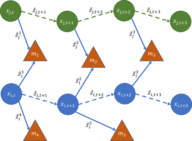
Figure 1: A factor graph representation of a multi-robot SLAM problem, where two robots, robot $i$ (blue circles) and $j$ (green circles), seek to jointly estimate a set of map features ${\{m_{1},m_{2},\cdots\}}$ (orange triangles) in addition to their own pose trajectory ${\{x_{i,t},x_{j,t},\ \forall t\}}$, from the set of odometry measurements ${\{\hat{z}_{i,t},\hat{z}_{j,t}\}}$ and observations of each map feature $k$ ${\{\breve{z}_{i}^{k},\breve{z}_{j}^{k}\}}$.

Although the first set of terms in the objective function of the optimization problem (6) is separable among the robots, the second set of terms is not. Consequently, the optimization problem must be reformulated for amenability to distributed optimization algorithms. Non-separability of the objective function arises from the coupling between the map features and the robot poses. To achieve separability of the objective function, we can introduce local copies of the variables corresponding to each feature, with an associated set of consensus (equality) constraints to ensure that the resulting problem remains equivalent to the original problem (6). The resulting problem takes the form

$$\underset{\mathbf{x},\hat{m}_{1},\hat{m}_{2},\cdots,\hat{m}_{N}}{\mathrm{minimize}} \sum_{i=1}^{N}\sum_{t=0}^{T-1}\|\bar{z}_{i,t}(x_{i,t},x_{i,t+1})-\hat{z}_{i,t+1}\|_{\Omega_{i,t}}^{2}$$ (7)

$$+\sum_{i=1}^{N}\sum_{k=1}^{M}\|\tilde{z}_{i}^{k}(x_{i},\hat{m}_{i,k})-\breve{z}_{i}^{k}\|_{\Lambda_{i,t}}^{2}$$

$$\mathrm{subject\ to} \hat{m}_{i}=\hat{m}_{j}\quad\forall(i,j)\in\mathcal{E},$$

where robot $i$ maintains $\hat{m}_{i}$, its local copy of the map $m$. The problem (7) is separable among the robots; in other words, its objective function can be expressed in the form

$$f(\mathbf{x},\hat{m}_{1},\hat{m}_{2},\cdots,\hat{m}_{N})=\sum_{i=1}^{N}f_{i}(x_{i},\hat{m}_{i}),$$ (8)

where

$$\begin{aligned} f_{i}(x_{i},\hat{m}_{i})&=\sum_{t=0}^{T-1}\|\bar{z}_{i,t}(x_{i,t},x_{i,t+1})-\hat{z}_{i,t+1}\|_{\Omega_{i,t}}^{2}\\ &+\sum_{k=1}^{M}\|\tilde{z}_{i}^{k}(x_{i},\hat{m}_{i,k})-\breve{z}_{i}^{k}\|_{\Lambda_{i,t}}^{2}\end{aligned}.$$ (9)

We can interpret the bundle adjustment problem similarly—in this case, the map features represent the scene geometry and the robot poses include the optical characteristics of the respective cameras. However, a challenge in applying this approach in unstructured environments is ensuring that multiple robots agree on the labels of the map landmarks. An alternative approach is pose graph optimization, which avoids explicitly estimating the map and instead uses relative pose measurements based on shared observations of features in the environment. In this perspective, multi-robot SLAM consists of a “front-end,” in which the robots process raw sensor measurements to generate relative pose measurements, and a “back-end,” in which robots find optimal robot poses given those relative pose measurements. The SLAM back-end is typically written as a pose graph optimization problem, where edges between nodes represent noisy relative pose estimates (which are obtained from the front-end) derived from raw sensor measurements. This pose graph optimization problem is a naturally separable optimization which is amenable to distributed optimization techniques, written as

$$\min_{\{(R_{i},\tau_{i})\}_{i=1}^{n}}\sum_{(i,j)\in\mathcal{E}}\frac{\omega_{ij}}{2}\|R_{j}-R_{i}\tilde{R}_{ij}\|^{2}_{F}+\frac{w_{ij}}{2}\|\tau_{j}-\tau_{i}-R_{i}\tilde{\tau}_{ij}\|^{2}_{2}$$

The pose graph optimization problem seeks to minimize the error between the expected relative pose obtained from the estimated poses and the measured relative pose, summed over all edges in the graph. The SLAM front end may be amenable to distributed optimization techniques as well, although this is an area of open research. Some existing distributed techniques that do not rely on distributed optimization have been proposed for the front-end, e.g., [7]. Refer to [8, 9, 10, 11] for additional details on SLAM and multi-robot SLAM.

Hence, distributed optimization algorithms can be readily applied to the graph-based SLAM problem in (7). Moreover, we note that a number of related robotics problems — including rotation averaging/synchronization and shape registration/alignment — can be similarly reformulated into a separable form and subsequently solved using distributed optimization algorithms [12, 13, 14, 15, 16, 17].

IV-B Multi-Robot Target Tracking

In the multi-robot target tracking problem, a group of robots collect measurements of an agent of interest (referred to as a target) and seek to collectively estimate the trajectory of the target. Multi-robot target tracking problems arise in many robotics applications ranging from environmental monitoring and surveillance to autonomous robotics applications such as autonomous driving, where the estimated trajectory of the target can be leveraged for scene prediction to enable safe operation. Figure 2 provides an illustration of the multi-robot target tracking problem where a group of four quadrotors make noisy observations of the flagged ground vehicle (the target). Each colored cone represents the region where each quadrotor can observe the vehicle, given the limited measurement range of the sensors onboard the quadrotor.

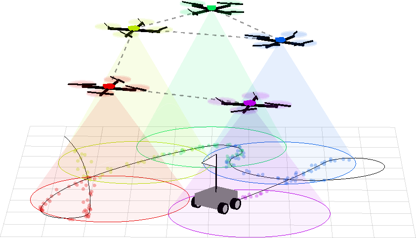
Figure 2: A multi-robot target tracking scenario, with four quadrotors (the robots) making noisy observations of the flagged ground vehicle (the target). The colored cones represent the regions where each quadrotor can observe the vehicle, given the limited measurement range of the sensors onboard each quadrotor.

Multi-robot target tracking problems can be posed as maximum a posterior (MAP) optimization problems where the robots seek to compute an estimate that maximizes the posterior distribution of the target’s trajectory given the set of all observations of the target made by the robots. When a model of the dynamics of target is available, denoted by ${g:\mathbb{R}^{n}\rightarrow\mathbb{R}^{n}}$, the resulting optimization problem takes the form

$$\underset{x}{\mathrm{minimize}} \sum_{t=0}^{T-1}\|x_{t+1}-g(x_{t})\|_{\Omega_{t}}^{2}$$ (10)

$$+\sum_{i=1}^{N}\sum_{t=0}^{T-1}\|y_{i,t}-h_{i}(x_{t})\|_{\Lambda_{i,t}}^{2},$$

where ${x_{t}\in\mathbb{R}^{n}}$ denotes the pose of the target at time $t$ and ${y_{i,t}\in\mathbb{R}^{m}}$ denotes robot $i$’s observation of the target at time $t$, over a duration of ${T+1}$ timesteps. We represent the trajectory of the target with ${x=\left[x_{0}^{\top},x_{1}^{\top},\cdots,x_{T}^{\top}\right]^{\top}}$. While the first term in the objective function corresponds to the error between the estimated state of the target at a subsequent timestep and its expected state based on a model of its dynamics, the second term corresponds to the error between the observations collected by each robot and the expected measurement computed from the estimated state of the target, where the function ${h_{i}:\mathbb{R}^{n}\rightarrow\mathbb{R}^{m}}$ denotes the measurement model of robot $i$. Further, the information matrices ${\Omega_{t}\in\mathbb{R}^{n\times n}}$ and ${\Lambda_{i,t}\in\mathbb{R}^{m\times m}}$ for the dynamics and measurement models, respectively, weight the contribution of each term in the objective function appropriately, reflecting prior confidence in the dynamics and measurement models. The MAP optimization problem in (10) is not separable, hence, not amenable to distributed optimization, in its current form, due to coupling in the objective function arising from $x$. Nonetheless, we can arrive at a separable optimization problem through a fairly straightforward reformulation [3]. We can assign a local copy of $x$ to each robot, with $\hat{x}_{i}$ denoting robot $i$’s local copy of $x$. The reformulated problem becomes

$$\underset{\hat{x}}{\mathrm{minimize}} \sum_{i=1}^{N}\sum_{t=0}^{T-1}\frac{1}{N}\|\hat{x}_{i,t+1}-g(\hat{x}_{i,t})\|_{\Omega_{t}}^{2}$$ (11)

$$+\sum_{i=1}^{N}\sum_{t=0}^{T-1}\|y_{i,t}-h_{i}(\hat{x}_{i,t})\|_{\Lambda_{i,t}}^{2}$$

$$\mathrm{subject\ to} \hat{x}_{i}=\hat{x}_{j}\quad\forall(i,j)\in\mathcal{E},$$

where ${\hat{x}=\left[\hat{x}_{1}^{\top},\hat{x}_{2}^{\top},\cdots,\hat{x}_{N}^{\top}\right]^{\top}}$. Following this reformulation, distributed optimization algorithms can be applied to compute an estimate of the trajectory of the target from (11).

IV-C Multi-Robot Task Assignment

In the multi-robot task assignment problem, we seek an optimal assignment of $N$ robots to $M$ tasks such that the total cost incurred in completing the specified tasks is minimized. However, we note that many task assignment problems consist of an equal number of tasks and robots. The standard task assignment problem has been studied extensively and is typically solved using the Hungarian method [18]. However, optimization-based methods have emerged as a competitive approach due to their amenability to task assignment problems with a diverse set of additional constraints, encoding individual preferences or other relevant problem information, making them a general-purpose approach.

The task assignment problem can be represented as a weighted bipartite graph: a graph whose vertices can be divide into two sets where no two nodes within a given set share an edge. Further, each edge in the graph has an associated weight. In task assignment problems, the edge weight $c_{i,j}$ represents the cost of assigning robot $i$ to task $j$. Figure 3 depicts a task assignment problem represented by a weighted bipartite graph, with three robots and three tasks. Each robot knows its task preferences only and does not know the task preferences of other robots. Equivalently, the task assignment problem can be formulated as an integer optimization problem. Many optimization-based methods solve a relaxation of the integer optimization problem. Generally, in problems with linear objective functions and affine constraints, these optimization-based methods are guaranteed to yield an optimal task assignment. The associated relaxed optimization problem takes the form

$$\underset{x}{\mathrm{minimize}} \sum_{i=1}^{N}c_{i}^{\top}x_{i}$$ (12)

$$\mathrm{subject\ to} \sum_{i=1}^{N}x_{i}=1_{M}$$

$$1_{M}^{\top}x_{i}=1$$

$$0\leq x\leq 1,$$

where ${x_{i}\in\mathbb{R}^{M}}$ denotes the optimization variable of robot $i$, representing its task assignment and ${x=\left[x_{1},x_{2},\cdots,x_{N}\right]}$. Although the objective function of (12) is separable, the optimization problem is not separable due to coupling of the optimization variables arising in the first constraint. We can obtain a separable problem, amenable to distributed optimization, by assigning a local copy of $x$ to each robot, resulting in the problem

$$\underset{\hat{x}}{\mathrm{minimize}} \sum_{i=1}^{N}c_{i}^{\top}\hat{x}_{i,i}$$ (13)

$$\mathrm{subject\ to} \sum_{i=1}^{N}\hat{x}_{i,i}=1_{M}$$

$$1_{M}^{\top}\hat{x}_{i,i}=1$$

$$0\leq\hat{x}_{i}\leq 1\quad\forall i\in\mathcal{V}$$

$$\hat{x}_{i}=\hat{x}_{j}\quad\forall(i,j)\in\mathcal{E}$$

where ${\hat{x}_{i}\in\mathbb{R}^{M\times N}}$ denotes robot $i$’s local copy of $x$ and ${\hat{x}=\left[\hat{x}_{0},\hat{x}_{1},\cdots,\hat{x}_{N}\right]}$. Although the reformulation in (13) is simple, it does not scale efficiently with the number of robots and tasks. A more efficient reformulation can be obtained by considering the dual formulation of the task assignment problem. For brevity, we omit a discussion of this approach in this paper and refer readers to [19, 20, 21] where this reformulation scheme is discussed in detail.

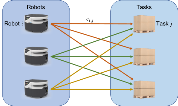
Figure 3: A multi-robot task assignment problem represented as a bipartite graph, with three (Fetch) robots and three tasks. An edge with weight $c_{i,j}$ between robot $i$ and task $j$ signifies the cost incurred by robot $i$ if it performs task $j$. In many problems, each robot’s task preferences (edge weights) is neither known by other robots nor accessible to these robots.

IV-D Collaborative Planning, Control, and Manipulation

Generally, in collaborative planning problems, we seek to compute state and control input trajectories that enable a group of robots to reach a desired state configuration from a specified initial state, while minimizing a trajectory cost and without colliding with other agents. The related multi-robot control problem involves computing a sequence of control inputs that enables a group of robots to track a desired reference trajectory or achieve some specified task such as manipulating an object collaboratively. Figure 4 shows a collaborative manipulation problem where three quadrotors move an object collaboratively. The dashed-line represents the reference trajectory for manipulating the load.

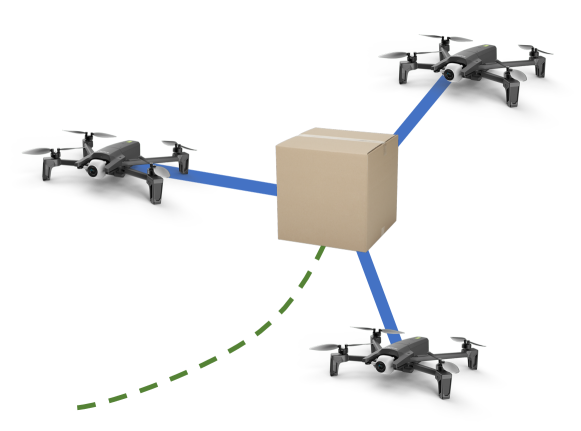
Figure 4: A multi-robot manipulation problem, with three quadrotors collaboratively manipulating a load rigidly attached to each quadrotor. The dashed-line represents the reference trajectory for manipulating the load.

Collaborative multi-robot planning, control, and manipulation problems have been well-studied, with a broad variety of methods devised for these problems. Among these methods, receding horizon or model predictive control (MPC) approaches have received notable attention due to their flexibility in encoding complex problem constraint and objectives. In MPC approaches, these multi-robot problems are formulated as optimization problems over a finite time duration at each timestep. The resulting optimization problem is solved to obtain a sequence of control inputs over the specified time duration; however, only the initial control input is applied by each robot at the current timestep. At the next timestep, a new optimization problem is formulated, from which a new sequence of control inputs is computed to obtain a new control input for that timestep. This process is repeated until completion of the task. At time $t$, the associated MPC optimization problem has the form

$$\underset{x,u}{\mathrm{minimize}} \sum_{i=1}^{N}f_{i}(x,u)$$ (14)

$$\mathrm{subject\ to} g(x,u)=0$$

$$h(x,u)\leq 0$$

$$x_{i,0}=\bar{x}_{i}\quad\forall i\in\mathcal{V}$$

where ${x_{i}\in\mathbb{R}^{n_{i}}}$ denotes robot $i$’s state trajectory, ${u_{i}\in\mathbb{R}^{m_{i}}}$ denotes its control input trajectory, and ${x=\left[x_{1}^{\top},x_{2}^{\top},\cdots,x_{N}^{\top}\right]^{\top}}$ with ${u=\left[u_{1}^{\top},u_{2}^{\top},\cdots,u_{N}^{\top}\right]^{\top}}$. The objective function of robot $i$, ${f_{i}:\mathbb{R}^{\bar{n}}\times\mathbb{R}^{\bar{m}}\rightarrow\mathbb{R}}$, is often quadratic, given by

$$f_{i}(x,u)=(x_{i}-\tilde{x}_{i})^{\top} Q_{i}(x_{i}-\tilde{x}_{i})$$ (15)

$$+(u_{i}-\tilde{u}_{i})^{\top}R_{i}(u_{i}-\tilde{u}_{i}),$$

where $\tilde{x}_{i}$ and $\tilde{u}_{i}$ denote the reference state and control input trajectory, respectively, ${Q_{i}\in\mathbb{R}^{n_{i}\times n_{i}}}$ and ${R_{i}\in\mathbb{R}^{m_{i}\times m_{i}}}$ denote the associated weight matrices for the terms in the objective function, ${\bar{n}=\sum_{i=1}^{N}n_{i}}$, and ${\bar{m}=\sum_{i=1}^{N}m_{i}}$. The dynamics function of the robots is encoded in ${g:\mathbb{R}^{\bar{n}}\times\mathbb{R}^{\bar{m}}\rightarrow\mathbb{R}^{\bar{n}}}$. Further, other equality constraints can be encoded in $g$. Inequality constraints, such as collision-avoidance constraints and other state or control input feasibility constraints, are encoded in ${h:\mathbb{R}^{\bar{n}}\times\mathbb{R}^{\bar{m}}\rightarrow\mathbb{R}^{l}}$. In addition, the first state variable of each agent is constrained to be equal to its initial state, denoted by $\bar{x}_{i}$. In each instance of the MPC optimization problem, the initial state $\bar{x}_{i}$ of robot $i$ is specified as its current state at that timestep. Note that the MPC optimization problem in (14) is not generally separable, depending on the equality and inequality constraints. However, a separable form of the problem can always be obtained by introducing local copies of the optimization variables that are coupled in (14). The functions $g$ and $h$ can also encode complementarity constraints for manipulation and locomotion problems that involve making and breaking rigid body contact [22]. In the extreme case, where the optimization variables are coupled in the objective function and equality and inequality constraints in (14), a suitable reformulation takes the form

$$\underset{\hat{x},\hat{u}}{\mathrm{minimize}} \sum_{i=1}^{N}f_{i}(\hat{x}_{i},\hat{u}_{i})$$ (16)

$$\mathrm{subject\ to} g(\hat{x}_{i},\hat{u}_{i})=0\quad\forall i\in\mathcal{V}$$

$$h(\hat{x}_{i},\hat{u}_{i})\leq 0\quad\forall i\in\mathcal{V}$$

$$\phi_{i}(\hat{x}_{i})=\bar{x}_{i}\quad\forall i\in\mathcal{V}$$

$$\hat{x}_{i}=\hat{x}_{j}\quad\forall(i,j)\in\mathcal{E},$$

where the function $\phi_{i}$ outputs the first state variable corresponding to robot $i$, given the input $\hat{x}_{i}$, which denotes robot $i$’s local copy of $x$. Similarly, $\hat{u}_{i}$ denotes robot $i$’s local copy of $u$, with ${\hat{x}=\left[\hat{x}_{1}^{\top},\hat{x}_{2}^{\top},\cdots,\hat{x}_{N}^{\top}\right]^{\top}}$ and ${\hat{u}=\left[\hat{u}_{1}^{\top},\hat{u}_{2}^{\top},\cdots,\hat{u}_{N}^{\top}\right]^{\top}}$. Distributed optimization algorithms [5, 23, 24] can be employed to solve the resulting MPC optimization problem in (16).

IV-E Multi-Robot Learning

Multi-robot learning entails the application of deep learning methods to approximate functions from data to solve multi-robot tasks, such as object detection, visual place recognition, monocular depth estimation, 3D mapping, and multi-robot reinforcement learning. Consider a general multi-robot supervised learning problem where we aim to minimize a loss function over labeled data collected by all the robots. We can write this as

$$\min_{\theta}\sum_{i=1}^{N}\sum_{(x_{ij},y_{ij})\in D_{i}}l(y_{i},f(x_{i};\theta)),$$

where $l(\cdot,\cdot)$ is the loss function, $(x_{ij},y_{ij})$ is data point $j$ collected by robot $i$ with feature vector $x_{ij}$ and label $y_{ij}$, $D_{i}$ is the set of data collected by robot $i$, $\theta$ are the neural network weights, and $f(x;\theta)$ is the neural network parameterized function we desire to learn. By creating local copies of the neural network weights $\theta_{i}$ and adding consensus constraints $\theta_{i}=\theta_{j}$, we can put problem in the form (5), so it is amenable to distributed optimization. We stress that this problem encompasses a large majority of problems in supervised learning. See [25] for an ADMM-based distributed optimization approach to solving this problem.

Beyond supervised learning, many multi-robot learning problems are formulated within the framework of reinforcement learning. In these problems, the robots learn a control policy by interacting with their environments by making sequential decisions. The underlying control policy, which drives these sequential decisions, is iteratively updated to optimize the performance of all agents on a specified objective using the information gathered by each robot during its interaction with its environment. Figure 5 illustrates the reinforcement learning paradigm, where a group of robots learn from experience. Each robot takes an action and receives an observation (and a reward), which provides information on the performance of its current control policy in achieving its specified objective.

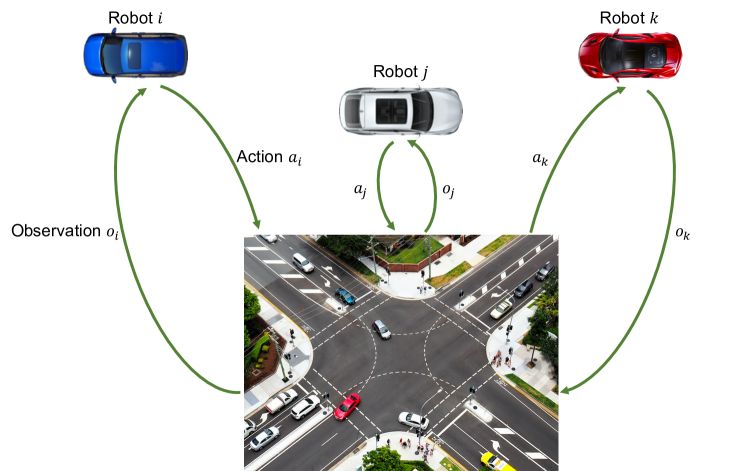
Figure 5: In multi-robot reinforcement learning problems, a group of robots compute a control policy from experience by making sequential decisions while interacting with their environment. Each robot takes an action and receives an observation (and a reward), which provides information on its performance in accomplishing a specified task.

Reinforcement learning approaches can be broadly categorized into value-based methods and policy-based methods. Value-based methods seek to compute an estimate of the optimal action-value function — the $Q$-function — which represents the expected discounted reward starting from a given state and taking a given action. An optimal policy can be extracted from the estimated $Q$-function by selecting the action that maximizes the value of the $Q$-function at a specified state. In deep value-based methods, deep neural networks are utilized in approximating the $Q$-function. In contrast, policy-based methods seek to find an optimal policy by directly searching over the space of policies. In deep policy-based methods, the control policy is parameterized using deep neural networks. In general, the agents seek to maximize the expected infinite-horizon discounted cumulative reward, which is posed as the optimization problem

$$\underset{\theta}{\mathrm{maximize}} \mathbb{E}_{\pi_{\theta}}\left[\sum_{t\geq 0}\gamma^{t}\sum_{i=1}^{N}R_{i}(s_{i,t},a_{i,t})\mid s_{i,0}=\bar{s}_{i}\right],$$ (17)

where $\pi_{\theta}$ denotes the control policy parameterized by $\theta$, ${\gamma\in\mathbb{R}}$ denotes the discount factor (${\gamma\in(0,1)}$), $s_{i,t}$ denotes the state of robot $i$ at time $t$, $a_{i,t}$ denotes its action at time $t$, $\bar{s}_{i}$ denotes its initial state, ${R_{i}:\mathcal{S}_{i}\times\mathcal{A}_{i}\rightarrow\mathbb{R}}$ denotes the reward function of robot $i$, and $N$ denotes the number of robots. The optimization problem in (17) is not separable in its current form. However, due to the linearity of the expectation operator, the optimization problem in (17) can be equivalently expressed as

$$\underset{\hat{\theta}_{1},\cdots,\hat{\theta}_{N}}{\mathrm{maximize}} \sum_{i=1}^{N}\mathbb{E}_{\pi_{\hat{\theta}_{i}}}\left[\sum_{t\geq 0}\gamma^{t}R_{i}(s_{i,t},a_{i,t})\mid s_{i,0}=\bar{s}_{i}\right]$$ (18)

$$\mathrm{subject\ to} \hat{\theta}_{i}=\hat{\theta}_{j}\quad\forall(i,j)\in\mathcal{E},$$

which is separable among the $N$ robots. Hence, the resulting problem can be readily solved using distributed optimization algorithms for reinforcement learning problems, such as distributed $Q$-learning and distributed actor-critic methods [26, 27, 28].

V Classes of Distributed Optimization Algorithms

In this section, we categorize distributed optimization algorithms into three broad classes — Distributed First-Order Methods, Distributed Sequential Convex Programming, and Alternating Direction Method of Multipliers — and provide a brief overview of each category, by considering a representative distributed algorithm within each category. In the subsequent discussion, we consider the separable optimization problem in (5). In the tutorial spirit of this paper, we first consider problems without the local equality and inequality constraint functions, $g_{i}$ and $h_{i}$. In the second paper in this series, we include these constraint functions, as we give a survey of more sophisticated distributed optimization algorithms.

Before describing the specific algorithms that solve distributed optimization problems, we first consider the general framework that all of these approaches share. Each algorithm progresses over discrete iterations $k=0,1,\dots$ until convergence. In general, each iteration consists of a communication step and a computation step. Besides assuming that each robot has the sole capability of evaluating its local objective function $f_{i}$, we also distinguish between the “internal” variables $\mathcal{P}_{i}^{(k)}$ that the robot computes at each iteration $k$ and the “communicated” variables $\mathcal{Q}_{i}^{(k)}$ that the robot communicates to its neighbors. Each algorithm also involves parameters $\mathcal{R}_{i}^{(k)}$, which generally require coordination among all of the robots but can typically be assigned before deployment of the system.

In distributed optimization, all the robots seek to collectively minimize the joint objective function in (5) while achieving consensus on a common set of minimizing optimization variables. In this paper, we distinguish between two distinct perspectives on how consensus between the robots is achieved. Distributed first-order methods and distributed sequential convex programming methods enforce the consensus (equality) constraints in (5) implicitly, while the alternating direction method of multipliers enforces these constraints explicitly.

V-A Distributed First-Order Algorithms

Gradient decent methods have been widely applied to solve broad classes of optimization problems. In general, these methods only require the computation of the gradient (i.e., the first derivative of the objective and constraint functions); hence, these methods are also referred to as first-order methods. When applied to (5), the updates to the optimization variable take the form

$$x^{(k+1)}=x^{(k)}-\alpha^{(k)}\nabla f(x^{(k)})$$ (19)

where $\alpha^{(k)}$ denotes a diminishing step-size and $\nabla f(x^{(k)})$ denotes the gradient of the objective function, given by

$$\nabla f(x)=\sum_{i\in\mathcal{V}}\nabla f_{i}(x).$$ (20)

From (20), computation of $\nabla f(x)$ requires knowledge of the objective function of all robots, which is unavailable to any individual robot, and thus requires aggregation of this information at a central node.

Distributed First-Order (DFO) algorithms provide alternative update schemes that circumvent this underlying challenge by enabling each robot to utilize only its local gradients, while communicating with its neighbors to reach consensus on a common solution. We can further categorize DFO methods into two broad subclasses: Adapt-Then-Combine (ATC) methods and Combine-Then-Adapt (CTA) methods, based on the relative order of the communication and computation procedures. In ATC methods, each robot updates its local optimization variable using its gradient prior to combining its local variable with that of its neighbors, with the update procedure given by

$$x_{i}^{(k+1)}=\sum_{j\in\mathcal{N}_{i}\cup\{i\}}w_{ij}(x_{j}^{(k)}-\alpha^{(k)}y_{j}^{(k)}),$$ (21)

where ${x_{j}^{(k)}\in\mathbb{R}^{n}}$ denotes the local variable of neighboring robot $j$ and $y_{j}^{(k)}$ denotes $j$’s local gradient $y_{j}^{(k)}=\nabla f_{j}(x_{j}^{(k)})$. Note that each robot updates its local variable $x_{i}^{(k+1)}$ using gradients from its one-hop neighborhood before communicating its local variable with its neighbors. The weight $w_{i,j}$ must be compatible with the underlying communication network, such that ${w_{i,j}=0}$ if robots $i$ and $j$ do not share a direct communication link, and the weighting matrix $W$ should be a stochastic matrix.

In contrast, in CTA methods, each robot combines its local variable with that of its neighbors prior to incorporating its local gradient, yielding the update procedure

$$x_{i}^{(k+1)}=\sum_{j\in\mathcal{N}_{i}\cup\{i\}}w_{ij}x_{j}^{(k)}-\alpha^{(k)}y_{i}^{(k)}.$$ (22)

In the simplest case, ${y_{i}^{(k)}=\nabla f_{i}(x_{i}^{(k)})}$, or more generally, ${y_{i}^{(k)}=\partial f_{i}(x_{i}^{(k)})}$ (where $\partial f_{i}$ denotes the subgradient of $f_{i}$), yielding the canonical distributed subgradient method [29]. This choice of ${y_{i}^{(k)}}$ necessitates the use of a diminishing step-size, which is often given by ${\alpha^{(k+1)}=\frac{\alpha^{(0)}}{\sqrt{k}}}$.

More sophisticated gradient tracking methods, for example DIGing [30], employ an estimate of the average gradient computed through dynamic average consensus with

$${y_{i}^{(k+1)}=\sum_{j\in\mathcal{N}_{i}\cup\{i\}}w_{ij}y_{j}^{(k)}+\left[\nabla f_{i}(x_{i}^{(k+1)})-\nabla f_{i}(x_{i}^{(k)})\right]},$$ (23)

which does not require a diminishing step-size. At initialization of the algorithm, all the robots select a common step-size. Further, robot $i$ initializes its local variables with ${x_{i}^{(0)}\in\mathbb{R}^{n}}$ and ${y_{i}^{(0)}=\partial f_{i}(x_{i}^{(0)})}$. Algorithm 1 summarizes the update procedures in the distributed gradient tracking method DIGing [30]. Many DFO methods impose additional restrictions on the weighting matrix. For example, DIGing requires a doubly-stochastic weighting matrix for undirected communication networks.

Initialization: $k\leftarrow 0$, ${x_{i}^{(0)}\in\mathbb{R}^{n}}$, ${y_{i}^{(0)}=\nabla f_{i}(x_{i}^{(0)})}$

Internal variables: $\mathcal{P}_{i}^{(k)}=\emptyset$

Communicated variables: $\mathcal{Q}_{i}^{(k)}=\left(x_{i}^{(k)},y_{i}^{k}\right)$

Parameters: $\mathcal{R}_{i}^{(k)}=\left(\alpha,w_{i}\right)$

do in parallel  $\forall i\in\mathcal{V}$

       Communicate $\mathcal{Q}_{i}^{(k)}$ to all $j\in\mathcal{N}_{i}$

       Receive $\mathcal{Q}_{j}^{(k)}$ from all $j\in\mathcal{N}_{i}$

$$x_{i}^{(k+1)} =\sum_{j\in\mathcal{N}_{i}\cup\{i\}}w_{ij}x_{j}^{(k)}-\alpha y_{i}^{(k)}$$

$$y_{i}^{(k+1)} =\sum_{j\in\mathcal{N}_{i}\cup\{i\}}w_{ij}y_{j}^{(k)}+\nabla f_{i}(x_{i}^{(k+1)})-\nabla f_{i}(x_{i}^{(k)})$$

      $k\leftarrow k+1$

while stopping criterion is not satisfied

Algorithm 1 DIGing

V-B Distributed Sequential Convex Programming

Sequential convex programming entails solving an optimization problem by computing a sequence of iterates, representing the solution of a series of approximations of the original problem. Newton’s method is a prime example of a sequential convex programming method. In Newton’s method, and more generally, quasi-newton methods, we take a quadratic approximation of the objective function at an operating point $x^{(k)}$, resulting in

$$\tilde{f}(x) =f(x^{(k)})+\nabla f(x^{(k)})^{\top}(x-x^{(k)})$$ (24)

$$\quad+\frac{1}{2}(x-x^{(k)})^{\top}H(x^{(k)})(x-x^{(k)}),$$

where $H(\cdot)$ denotes the Hessian of the objective function, $\nabla^{2}f$, or its approximation. Subsequently, we compute a solution to the quadratic program, given by

$$x^{(k+1)}=x^{(k)}-H\bigl{(}x^{(k)}\bigr{)}^{-1}\nabla f(\tilde{x}),$$ (25)

which requires centralized evaluation of the gradient and Hessian of the objective function. Distributed Sequential Programming enable each robot to compute a local estimate of the gradient and Hessian of the objective function, and thus allows for the local execution of the update procedures. We consider the NEXT algorithm [31] to illustrate this class of distributed optimization algorithms. We assume that each robot uses a quadratic approximation of the optimization problem as its convex surrogate model $U(\cdot)$. In NEXT, each robot maintains an estimate of the average gradient of the objective function, as well as an estimate of the gradient of the objective function excluding its local component (e.g., ${\sum_{j\neq i}f_{j}(x_{i})}$ for robot $i$). At a current iterate ${x_{i}^{(k)}}$, robot $i$ creates a quadratic approximation of the optimization problem, given by

$$\underset{\tilde{x}_{i}}{\mathrm{minimize}} \left(\nabla f_{i}(x_{i}^{(k)})+{\tilde{\pi}}_{i}^{(k)}\right)^{\top}\bigl{(}\tilde{x}_{i}-x_{i}^{(k)}\bigr{)}$$ (26)

$$\quad+\frac{1}{2}\bigl{(}\tilde{x}_{i}-x_{i}^{(k)}\bigr{)}^{\top}H_{i}\bigl{(}x_{i}^{(k)}\bigr{)}\bigl{(}\tilde{x}_{i}-x_{i}^{(k)}\bigr{)},$$

where ${\tilde{\pi}}_{i}^{(k)}$ denotes robot $i$’s estimate of the gradient of ${\sum_{j\neq i}f_{j}(x_{i})}$ at $x_{i}^{(k)}$, which can be solved locally. Each robot computes a weighted combination of its current iterate and the solution of (26), given by the procedure

$$z_{i}^{(k)}=x_{i}^{(k)}+\alpha^{(k)}\left({\tilde{x}}_{i}^{(k)}-x_{i}^{(k)}\right),$$ (27)

where ${\alpha^{(k)}\in(0,1)}$ denotes a diminishing step-size. Subsequently, robot $i$ computes its next iterate by taking a weighted combination of its local estimate $z_{i}^{(k)}$ with that of its neighbors via the procedure

$$x_{i}^{(k+1)}=\sum_{j\in\mathcal{N}_{i}\cup\{i\}}w_{ij}z_{j}^{(k)},$$ (28)

for consensus on a common solution of the original optimization problem, where the weight $w_{i,j}$ must be compatible with the underlying communication network. In addition, robot $i$ updates its estimates of the average gradient of the objective function, denoted by $y_{i}$, using dynamic average consensus, given by

$$y_{i}^{(k+1)}=\sum_{j\in\mathcal{N}_{i}\cup\{i\}}w_{ij}y_{j}^{(k)}+\left[\nabla f_{i}(x_{i}^{(k+1)})-\nabla f_{i}(x_{i}^{(k)})\right],$$ (29)

as well as ${\tilde{\pi}}_{i}^{(k)}$ using the procedure

$${\tilde{\pi}}_{i}^{(k+1)}=N\cdot y_{i}^{(k+1)}-\nabla f_{i}(x_{i}^{(k+1)}).$$ (30)

Each agent initializes its local variables with ${x_{i}^{(0)}\in\mathbb{R}^{n}}$, ${y_{i}^{(0)}=\nabla f_{i}(x_{i}^{(0)})}$, and ${{\tilde{\pi}}_{i}^{(k+1)}=Ny_{i}^{(0)}-\nabla f_{i}(x_{i}^{(0)})}$, prior to executing the above update procedures. Algorithm 2 summarizes the update procedures in NEXT [31].

Initialization: $k\leftarrow 0$, ${x_{i}^{(0)}\in\mathbb{R}^{n}}$, ${y_{i}^{(0)}=\nabla f_{i}(x_{i}^{(0)})}$, Initialization: ${{\tilde{\pi}}_{i}^{(k+1)}=Ny_{i}^{(0)}-\nabla f_{i}(x_{i}^{(0)})}$

Internal variables: $\mathcal{P}_{i}=\left(x_{i}^{(k)},\tilde{x}_{i}^{(k)},{\tilde{\pi}}_{i}^{(k)}\right)$

Communicated variables: $\mathcal{Q}_{i}^{(k)}=\left(z_{i}^{(k)},y_{i}^{(k)}\right)$

Parameters: $\mathcal{R}_{i}^{(k)}=\left(\alpha^{(k)},w_{i},U(\cdot),\mathcal{K}\right)$

do in parallel  $\forall i\in\mathcal{V}$

      

$${\tilde{x}}_{i}^{(k)} =\operatorname*{argmin}_{x\in\mathcal{K}}\ U\left(x;x_{i}^{(k)},{\tilde{\pi}}_{i}^{(k)}\right)$$

$$z_{i}^{(k)} =x_{i}^{(k)}+\alpha^{(k)}\left({\tilde{x}}_{i}^{(k)}-x_{i}^{(k)}\right)$$

Communicate $\mathcal{Q}_{i}^{(k)}$ to all $j\in\mathcal{N}_{i}$

       Receive $\mathcal{Q}_{j}^{(k)}$ from all $j\in\mathcal{N}_{i}$

$$x_{i}^{(k+1)} =\sum_{j\in\mathcal{N}_{i}\cup\{i\}}w_{ij}z_{j}^{(k)}$$

$$y_{i}^{(k+1)} =\sum_{j\in\mathcal{N}_{i}\cup\{i\}}w_{ij}y_{j}^{(k)}$$

$$\qquad+\left[\nabla f_{i}(x_{i}^{(k+1)})-\nabla f_{i}(x_{i}^{(k)})\right]$$

$${\tilde{\pi}}_{i}^{(k+1)} =N\cdot y_{i}^{(k+1)}-\nabla f_{i}(x_{i}^{(k+1)})$$

      $k\leftarrow k+1$

while stopping criterion is not satisfied

Algorithm 2 NEXT

V-C Alternating Direction Method of Multipliers

The alternating direction method of multipliers (ADMM) belongs to the class of optimization algorithms referred to as the method of multipliers (or augmented Lagrangian methods), which compute a primal-dual solution pair of a given optimization problem. The method of multipliers proceeds in an alternating fashion: the primal iterates are updated as minimizers of the augmented Lagrangian, and subsequently, the dual iterates are updated via dual (gradient) ascent on the augmented Lagrangian. The procedure continues iteratively until convergence or termination. The augmented Lagrangian of the problem in (5) (with only the consensus constraints) is given by

$$\mathcal{L}_{a}(\mathbf{x},q) =\sum_{i=1}^{N}f_{i}(x_{i})$$ (31)

$$\enspace+\sum_{i=1}^{N}\sum_{j\in\mathcal{N}_{i}}\left(q_{i,j}^{\top}(x_{i}-x_{j})+\frac{\rho}{2}\|x_{i}-x_{j}\|_{2}^{2}\right),$$

where $q_{i,j}$ represents a dual variable for the consensus constraints between robots $i$ and $j$, ${q=\left[q_{i,j}^{\top},\ \forall(i,j)\in\mathcal{E}\right]^{\top}}$, and ${\mathbf{x}=\left[x_{1}^{\top},x_{2}^{\top},\cdots,x_{N}^{\top}\right]^{\top}}$. The parameter ${\rho>0}$ represents a penalty term on the violations of the consensus constraints. Generally, the method of multipliers computes the minimizer of the augmented Lagrangian with respect to the joint set of optimization variables, which hinders distributed computation. In contrast, in the alternating direction method of multipliers, the minimization procedure is performed block-component-wise, enabling parallel, distributed computation of the minimization subproblem in the consensus problem. However, many ADMM algorithms still require some centralized computation, rendering them not fully-distributed in multi-robot mesh network sense that we consider in this paper.

We focus here on ADMM algorithms that are distributed over robots in a mesh network, with each robot executing the same set of distributed steps. We specifically consider the consensus alternating direction method of multipliers (C-ADMM) [32] as a representative algorithm within this category. C-ADMM introduces auxiliary optimization variables into the consensus constraints in (5) to enable fully-distributed update procedures. The primal update procedure of robot $i$ takes the form

$$x_{i}^{(k+1)} =\operatorname*{argmin}_{x_{i}}\Bigg{\{}f_{i}(x_{i})+x_{i}^{\top}y_{i}^{(k)}$$ (32)

$$\hskip 50.00008pt+\rho\sum_{j\in\mathcal{N}_{i}}\left\|x_{i}-\frac{1}{2}\left(x_{i}^{(k)}+x_{j}^{(k)}\right)\right\|^{2}_{2}\Bigg{\}},$$

which only requires information locally available to robot $i$, including information received from its neighbors (i.e., ${x_{j}^{k},\ \forall j\in\mathcal{N}_{i}}$). As a result, this procedure can be executed locally by each agent, in parallel. After communicating with its neighbors, each robot updates its local dual variable using the procedure

$$y_{i}^{(k+1)}=y_{i}^{(k)}+\rho\sum_{j\in\mathcal{N}_{i}}\left(x_{i}^{(k+1)}-x_{j}^{(k+1)}\right),$$ (33)

where $y_{i}$ denotes the composite dual variable of robot $i$, corresponding to the consensus constraints between robot $i$ and its neighbors, which is initialized to zero. Algorithm 3 summarizes the update procedures in C-ADMM [32].

Initialization: $k\leftarrow 0$, ${x_{i}^{(0)}\in\mathbb{R}^{n}}$, ${y_{i}^{(0)}=0}$

Internal variables: $\mathcal{P}_{i}^{(k)}=y_{i}^{(k)}$

Communicated variables: $\mathcal{Q}_{i}^{(k)}=x_{i}^{(k)}$

Parameters: $\mathcal{R}_{i}^{(k)}=\rho$

do in parallel  $\forall i\in\mathcal{V}$

      

$$x_{i}^{(k+1)}=\operatorname*{argmin}_{x_{i}}\Bigg{\{}f_{i}(x_{i})+x_{i}^{\top}y_{i}^{(k)}\cdots$$

$$\hskip 60.00009pt+\rho\sum_{j\in\mathcal{N}_{i}}\left\|x_{i}-\frac{1}{2}\left(x_{i}^{(k)}+x_{j}^{(k)}\right)\right\|^{2}_{2}\Bigg{\}}$$

Communicate $\mathcal{Q}_{i}^{(k)}$ to all $j\in\mathcal{N}_{i}$

       Receive $\mathcal{Q}_{j}^{(k)}$ from all $j\in\mathcal{N}_{i}$

$$y_{i}^{(k+1)} =y_{i}^{(k)}+\rho\sum_{j\in\mathcal{N}_{i}}\left(x_{i}^{(k+1)}-x_{j}^{(k+1)}\right)$$

      $k\leftarrow k+1$

while stopping criterion is not satisfied

Algorithm 3 C-ADMM

VI Distributed Multi-drone Vehicle Tracking: A Case Study

Many robotics problems have a distributed structure, although this structure might not be immediately apparent. In many cases, applying distributed optimization methods requires reformulating the original problem into a separable form that allows for distributed computation of the problem variables locally by each robot. This reformulation often involves the introduction of additional problem variables local to each robot with an associated set of constraints relating the local variables between the robots. We illustrate this procedure using multi-drone vehicle target tracking as a case study in simulation. We note that the same principles apply to a broad class of robotics problems as we have outlined in Sec. IV. In addition, we implement the distributed optimization algorithm C-ADMM on hardware, to demonstrate the deployment of distributed optimization algorithms on hardware.

VI-A Simulation Study

In this simulation, we consider a distributed multi-drone vehicle target tracking problem in which robots connected by a communication graph, $\mathcal{G}=(\mathcal{V},\mathcal{E})$, each record range-limited linear measurements of a moving target, and seek to collectively estimate the target’s entire trajectory. We assume that each drone can communicate locally with nearby drones over the undirected communication graph $\mathcal{G}$. The drones all share a linear model of the target’s dynamics as

$$x_{t+1}=A_{t}x_{t}+w_{t},$$ (34)

where $x_{t}\in\mathbb{R}^{4}$ represents the position and velocity of the target in some global frame at time $t$, $A_{t}$ is the dynamics matrix associated with a linear model of the target’s dynamics, and $w_{t}\sim\mathcal{N}(0,Q_{t})$ represents process noise (including the unknown control inputs to the target). Restricting our case study to a linear target model in this tutorial ensures that the underlying optimization problem is convex, leading to strong convergence guarantees and robust numerical properties for our algorithm. A more expressive nonlinear model can also be used, but this requires a more sophisticated distributed optimization algorithm with more challenging numerical properties. At every time-step when the target is sufficiently close to a drone $i$ (which we denote by $t\in\mathcal{T}_{i}$), that robot collects an observation according to the linear measurement model

$$y_{i,t}=C_{i,t}x_{t}+v_{i,t}\>,$$ (35)

where $y_{i,t}\in\mathbb{R}^{2}$ is a positional measurement, $C_{i,t}$ is the measurement matrix of drone $i$, and $v_{i,t}\sim\mathcal{N}(0,R_{i,t})$ is measurement noise. We again assume a linear measurement model to keep this case study as simple as possible. A nonlinear model can also be used.

All of the drones have the same model for the prior distribution of the initial state of the target $\mathcal{N}(\bar{x}_{0},\bar{P}_{0})$, where ${\bar{x}_{0}\in\mathbb{R}^{4}}$ denotes the mean and ${\bar{P}_{0}\in\mathbb{R}^{4\times 4}}$ denotes the covariance. The global cost function is of the form

$$f(x)= \|x_{0}-\bar{x}_{0}\|_{\bar{P}_{0}^{-1}}^{2}+\sum_{t=1}^{T-1}\|x_{t+1}-A_{t}x_{t}\|_{Q_{t}^{-1}}^{2}$$ (36)

$$+\sum_{i\in\mathcal{V}}\sum_{t\in\mathcal{T}_{i}}\|y_{i,t}-C_{i,t}x_{t}\|_{R^{-1}}^{2},$$

while the local cost function for drone $i$ is

$$f_{i}(x)= \frac{1}{N}\|x_{0}-\bar{x}_{0}\|_{\bar{P}_{0}^{-1}}^{2}+\sum_{t=1}^{T-1}\frac{1}{N}\|x_{t+1}-A_{t}x_{t}\|_{Q_{t}^{-1}}^{2}$$ (37)

$$+\sum_{t\in\mathcal{T}_{i}}\|y_{i,t}-C_{i,t}x_{t}\|_{R^{-1}}^{2}.$$

In our results, we consider only a batch solution to the problem (finding the full trajectory of the target given each robot’s full set of measurements). Methods for performing the estimate in real-time through filtering and smoothing steps have been well studied, both in the centralized and distributed case [33]. An extended version of this multi-robot tracking problem is solved with distributed optimization in [3]. A rendering of a representative instance of this multi-robot tracking problem is shown in Figure 2.

In Figures 6 and 7, several distributed optimization algorithms are compared on an instance of the distributed multi-drone vehicle tracking problem. For this problem instance, 10 simulated drones seek to estimate the target’s trajectory over 16 time steps resulting in a decision variable dimension of $n=64$. We compare four distributed optimization methods which we consider to be representative of the taxonomic classes outlined in the sections above: C-ADMM [32], EXTRA [34], DIGing [30], and NEXT-Q [31]. Figure 6 shows that C-ADMM and EXTRA have similar fast convergence rates per iteration while DIGing and NEXT-Q are 4 and 15 times slower respectively to converge below an MSE of $10^{-6}$. The step-size hyperparameters for each method are computed by Golden Section Search (GSS) (for NEXT-Q, which uses a two parameter decreasing step-size, we fix one according to the values recommended in [31]).

We note that tuning is essential for achieving robust and efficient convergence with most distributed optimization algorithms. Figure 7 shows the sensitivity of these methods to variation in step-size, and highlights that three of the methods (all except C-ADMM) become divergent for certain subsets of the tested hyperparameter space. While C-ADMM seems to be the most effective algorithm in this problem instance, we note that other algorithms may have properties that are advantageous in other instances of this problem or other problems. For example, C-ADMM is known to require tight synchronization among the robots (or the computing nodes, more generally). If a robot misses a message or if robot clocks are not precisely synchronized, C-ADMM can perform poorly. First order methods, such as DIGing, tend to be more robust to asynchronicity, for example, and modifying these algorithms totolerate real-world challenges such as asynchronicity remains an area of active research. We discuss such issues in the second paper in this series.

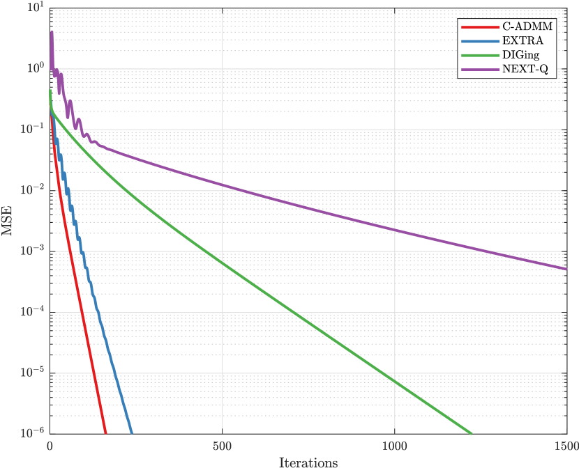
Figure 6: Mean Square Error (MSE) per iteration on a distributed multi-drone vehicle target tracking problem with $N=10$ and $n=64$.

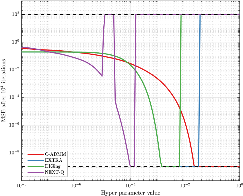
Figure 7: Step-size hyperparameter sensitivity sweep on a distributed multi-drone vehicle target tracking problem for $N=10$ and $n=64$. The dashed lines are thresholds for divergence (top) and convergence (bottom) in terms of MSE after $10^{4}$ decision variable updates.

VI-B Hardware Implementation

In this section, we discuss our implementation of the C-ADMM algorithm on hardware. Each robot is equipped with local computational resources and communication hardware necessary for peer-to-peer communication with other neighboring robots. In the following discussion, we provide details of the hardware platform, the underlying communication network between robots, and the optimization problem considered in this section.

We consider the linear least-squares optimization problem

$$\min_{p}\sum_{i=1}^{N}(G_{i}p-z_{i})^{\top}M_{i}(G_{i}p-z_{i}),$$ (38)

with the optimization variable ${p\in\mathbb{R}^{32}}$, ${G_{i}\in\mathbb{R}^{m_{i}\times 32}}$, ${M_{i}\in\mathbb{R}^{m_{i}\times m_{i}}}$, ${z_{i}\in\mathbb{R}^{m_{i}}}$, and ${N=3}$ robots, where $m_{i}$ depends on the number of measurements available to robot $i$. In this experiment, we have ${m_{1}=3268}$, ${m_{2}=5422}$, and ${m_{3}=3528}$. We implement C-ADMM to solve the problem, with a state size consisting of $32$ floating-point variables.

The core communication infrastructure that we use are Digi XBee DigiMesh 2.4 radio frequency mesh networking modules which allow for peer-to-peer communication between robots. Local computation for each robot is performed using Raspberry Pi 4B single board computers. The lower level mesh network is managed by the DigiMesh software, and we interact with it through XBee Python Library.

We utilize the neighbor discovery Application Programming Interface (API) provided by Digi International to enable each robot to identify other neighboring robots. This approach resulted in a fully-connected communication network, considering the XBee radios have an indoor range of up to $90$m and an outdoor range of up to $1500$m. The XBee modules used in our experiments have a maximum payload size of $92$ bytes. However, the local variable of each robot in our experiment consists of $32$ floating-point variables, which exceeds the maximum payload size that can be transmitted by the XBee radios at each broadcast round, presenting a communication challenge. To overcome this challenge, we break up the local variables into a series of packets of size $92$ bytes and perform multiple broadcast rounds. We note, however, that other approaches could be employed to overcome the limited communication bandwidth of the XBee radios, including utilizing quantization-based distributed optimization methods.

We set the penalty parameter in C-ADMM to a value of $5$ and do not perform a comprehensive search for the penalty parameter. In our experiments, we noticed that this value of the penalty parameter provided suitable performance. Noting that C-ADMM requires synchronous updates, we ensure that the local clocks of all robots remain synchronized in our experiments using a barrier strategy, which prevents each robot from advancing to the next iteration of C-ADMM until all other robots have completed the current iteration. In Figure 8, we show the convergence error between the iterates of each robot and the global solution, which is obtained by aggregating the local data of all robots and then computing the solution centrally. The convergence errors of all the robots iterates overlap in the figure, with the error decreasing below $10^{-5}$ within $250$ iterations, showing convergence of the local iterates of each robot to the optimal solution.

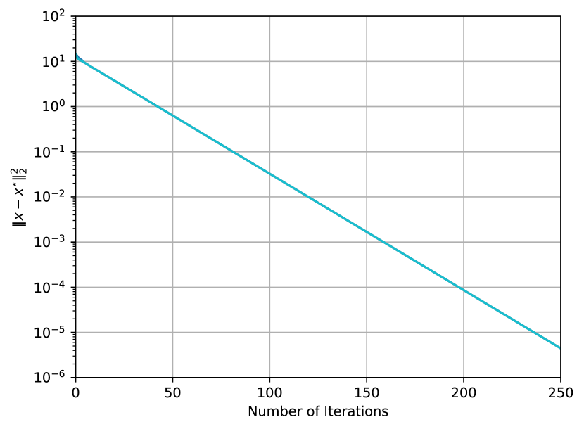
Figure 8: Convergence of the iterates computed by each robot using C-ADMM, implemented on hardware, on the optimization problem with three robots in (38). The convergence errors of all the robots overlap in the figure.

VII Conclusion

In this tutorial, we have demonstrated that a number of canonical problems in multi-robot systems can be formulated and solved through the framework of distributed optimization. We have identified three broad classes of distributed optimization algorithms: distributed first-order methods, distributed sequential convex programming methods, and the alternating direction method of multipliers (ADMM). Further, we have described the optimization techniques employed by the algorithms within each category, providing a representative algorithm for each category. In addition, we have demonstrated the application of distributed optimization in simulation, on a distributed multi-drone vehicle tracking problems, and on hardware, showing the effectiveness of distributed optimization algorithms. However, important challenges remain in developing distributed algorithms for constrained, non-convex robotics problems, and algorithms tailored to the limited computation and communication resources of robot platforms, which we discuss in greater detail in the second paper in this series [35].

References

- [1] R. T. Rockafellar, “Monotone operators and the proximal point algorithm,” SIAM journal on control and optimization, vol. 14, no. 5, pp. 877–898, 1976.
- [2] J. N. Tsitsiklis, “Problems in decentralized decision making and computation.” Massachusetts Inst of Tech Cambridge Lab for Information and Decision Systems, Tech. Rep., 1984.
- [3] O. Shorinwa, J. Yu, T. Halsted, A. Koufos, and M. Schwager, “Distributed multi-target tracking for autonomous vehicle fleets,” in 2020 IEEE International Conference on Robotics and Automation (ICRA). IEEE, 2020, pp. 3495–3501.
- [4] H.-T. Wai, Z. Yang, Z. Wang, and M. Hong, “Multi-agent reinforcement learning via double averaging primal-dual optimization,” in Advances in Neural Information Processing Systems, 2018, pp. 9649–9660.
- [5] J. Bento, N. Derbinsky, J. Alonso-Mora, and J. S. Yedidia, “A message-passing algorithm for multi-agent trajectory planning,” in Advances in neural information processing systems, 2013, pp. 521–529.
- [6] L.-L. Ong, T. Bailey, H. Durrant-Whyte, and B. Upcroft, “Decentralised particle filtering for multiple target tracking in wireless sensor networks,” in 2008 11th International Conference on Information Fusion. IEEE, 2008, pp. 1–8.
- [7] T. Cieslewski and D. Scaramuzza, “Efficient decentralized visual place recognition using a distributed inverted index,” IEEE Robotics and Automation Letters, vol. 2, no. 2, pp. 640–647, 2017.
- [8] H. Durrant-Whyte and T. Bailey, “Simultaneous localization and mapping: part i,” IEEE robotics & automation magazine, vol. 13, no. 2, pp. 99–110, 2006.
- [9] T. Bailey and H. Durrant-Whyte, “Simultaneous localization and mapping (slam): Part ii,” IEEE robotics & automation magazine, vol. 13, no. 3, pp. 108–117, 2006.
- [10] G. Grisetti, R. Kümmerle, C. Stachniss, and W. Burgard, “A tutorial on graph-based slam,” IEEE Intelligent Transportation Systems Magazine, vol. 2, no. 4, pp. 31–43, 2010.
- [11] A. Ahmad, G. D. Tipaldi, P. Lima, and W. Burgard, “Cooperative robot localization and target tracking based on least squares minimization,” in 2013 IEEE International Conference on Robotics and Automation. IEEE, 2013, pp. 5696–5701.
- [12] V.-L. Dang, B.-S. Le, T.-T. Bui, H.-T. Huynh, and C.-K. Pham, “A decentralized localization scheme for swarm robotics based on coordinate geometry and distributed gradient descent,” in MATEC Web of Conferences, vol. 54. EDP Sciences, 2016, p. 02002.
- [13] N. A. Alwan and A. S. Mahmood, “Distributed gradient descent localization in wireless sensor networks,” Arabian Journal for Science and Engineering, vol. 40, no. 3, pp. 893–899, 2015.
- [14] M. Todescato, A. Carron, R. Carli, and L. Schenato, “Distributed localization from relative noisy measurements: A robust gradient based approach,” in 2015 European Control Conference (ECC). IEEE, 2015, pp. 1914–1919.
- [15] R. Tron and R. Vidal, “Distributed 3-d localization of camera sensor networks from 2-d image measurements,” IEEE Transactions on Automatic Control, vol. 59, no. 12, pp. 3325–3340, 2014.
- [16] A. Sarlette and R. Sepulchre, “Consensus optimization on manifolds,” SIAM Journal on Control and Optimization, vol. 48, no. 1, pp. 56–76, 2009.
- [17] K.-K. Oh and H.-S. Ahn, “Distributed formation control based on orientation alignment and position estimation,” International Journal of Control, Automation and Systems, vol. 16, no. 3, pp. 1112–1119, 2018.
- [18] H. W. Kuhn, “The hungarian method for the assignment problem,” Naval research logistics quarterly, vol. 2, no. 1-2, pp. 83–97, 1955.
- [19] R. N. Haksar, O. Shorinwa, P. Washington, and M. Schwager, “Consensus-based admm for task assignment in multi-robot teams,” in The International Symposium of Robotics Research. Springer, 2019, pp. 35–51.
- [20] L. Liu and D. A. Shell, “Optimal market-based multi-robot task allocation via strategic pricing.” in Robotics: Science and Systems, vol. 9, no. 1, 2013, pp. 33–40.
- [21] S. Giordani, M. Lujak, and F. Martinelli, “A distributed algorithm for the multi-robot task allocation problem,” in International conference on industrial, engineering and other applications of applied intelligent systems. Springer, 2010, pp. 721–730.
- [22] O. Shorinwa and M. Schwager, “Distributed contact-implicit trajectory optimization for collaborative manipulation,” in 2021 International Symposium on Multi-Robot and Multi-Agent Systems (MRS). IEEE, 2021, pp. 56–65.
- [23] L. Ferranti, R. R. Negenborn, T. Keviczky, and J. Alonso-Mora, “Coordination of multiple vessels via distributed nonlinear model predictive control,” in 2018 European Control Conference (ECC). IEEE, 2018, pp. 2523–2528.
- [24] O. Shorinwa and M. Schwager, “Scalable collaborative manipulation with distributed trajectory planning,” in Proceedings of IEEE/RSJ International Conference on Intelligent Robots and Systems. IROS’20, vol. 1. IEEE, 2020, pp. 9108–9115.
- [25] J. Yu, J. A. Vincent, and M. Schwager, “DiNNO: Distributed neural network optimization for multi-robot collaborative learning,” IEEE Robotics and Automation Letters, vol. 7, no. 2, pp. 1896–1903, 2022.
- [26] K. Zhang, Z. Yang, H. Liu, T. Zhang, and T. Basar, “Fully decentralized multi-agent reinforcement learning with networked agents,” in International Conference on Machine Learning. PMLR, 2018, pp. 5872–5881.
- [27] Y. Zhang and M. M. Zavlanos, “Distributed off-policy actor-critic reinforcement learning with policy consensus,” in 2019 IEEE 58th Conference on Decision and Control (CDC). IEEE, 2019, pp. 4674–4679.
- [28] A. OroojlooyJadid and D. Hajinezhad, “A review of cooperative multi-agent deep reinforcement learning,” arXiv preprint arXiv:1908.03963, 2019.
- [29] A. Nedic and A. Ozdaglar, “On the rate of convergence of distributed subgradient methods for multi-agent optimization,” in IEEE Conference on Decision and Control. IEEE, 2007, pp. 4711–4716.
- [30] A. Nedic, A. Olshevsky, and W. Shi, “Achieving geometric convergence for distributed optimization over time-varying graphs,” SIAM Journal on Optimization, vol. 27, no. 4, pp. 2597–2633, 2017.
- [31] P. Di Lorenzo and G. Scutari, “NEXT: In-network nonconvex optimization,” IEEE Transactions on Signal and Information Processing over Networks, vol. 2, no. 2, pp. 120–136, 2016.
- [32] G. Mateos, J. A. Bazerque, and G. B. Giannakis, “Distributed sparse linear regression,” IEEE Transactions on Signal Processing, vol. 58, no. 10, pp. 5262–5276, 2010.
- [33] R. Olfati-Saber, “Distributed Kalman filtering for sensor networks,” in 2007 46th IEEE Conference on Decision and Control. IEEE, 2007, pp. 5492–5498.
- [34] W. Shi, Q. Ling, G. Wu, and W. Yin, “EXTRA: An exact first-order algorithm for decentralized consensus optimization,” SIAM Journal on Optimization, vol. 25, no. 2, pp. 944–966, 2015.
- [35] O. Shorinwa, T. Halsted, J. Yu, and M. Schwager, “Distributed Optimization Methods for Multi-Robot Systems: Part II — A Survey,” 2023.