Multi-compartment poroelastic models of perfused biological soft tissues: implementation in FEniCSx

Abstract

Soft biological tissues demonstrate strong time-dependent and strain-rate mechanical behavior, arising from their intrinsic visco-elasticity and fluid-solid interactions (especially at sufficiently large time scales). The time-dependent mechanical properties of soft tissues influence their physiological functions and are linked to several pathological processes. Poro-elastic modeling represents a promising approach because it allows the integration of multiscale/multiphysics data to probe biologically relevant phenomena at a smaller scale and embeds the relevant mechanisms at the larger scale. The implementation of multi-phasic flow poro-elastic models however is a complex undertaking, requiring extensive knowledge. The open-source software FEniCSx Project provides a novel tool for the automated solution of partial differential equations by the finite element method. This paper aims to provide the required tools to model the mixed formulation of poro-elasticity, from the theory to the implementation, within FEniCSx. Several benchmark cases are studied. A column under confined compression conditions is compared to the Terzaghi analytical solution, using the L2-norm. An implementation of poro-hyper-elasticity is proposed. A bi-compartment column is compared to previously published results (Cast3m implementation). For all cases, accurate results are obtained in terms of a normalized Root Mean Square Error (RMSE). Furthermore, the FEniCSx computation is found three times faster than the legacy FEniCS one. The benefits of parallel computation are also highlighted.

Implementation of poro-elastic formulations within FEniCSx.

Single and double compartment columns are modeled.

Elastic and hyper-elastic solid scaffold are computed.

Fast and accurate computation is obtained.

1 Introduction

Numerous biomechanical problems aim to reproduce the behavior of a deformable solid matrix that experiences flow-induced strain such as the brain (Budday et al. [1], Hosseini-Farid et al. [2], Franceschini et~al. [3], Urcun et~al. [4]), muscle tissues (Lavigne et~al. [5]), tumors (Sciumè et~al. [6], Sciumè [7], Oftadeh et~al. [8]), articular cartilages (Ateshian [9]) and lumbar inter-vertebral discs (Argoubi and Shirazi-Adl [10]). The time-dependent mechanical properties of soft tissues influence their physiological functions and are linked to several pathological processes. Although a fluid-structure interaction (FSI) problem, the number, and range of fluid flows are generally so vast that the direct approach of a defined boundary between fluid and solid is impossible to apply, as it requires an exponential computational cost at the organ scale with the requirement of extensive data acquisition at the micro-scale. In these cases, homogenization and statistical treatment of the material-fluid system is possibly the only way forward. A prominent technique of this type is that of poro-elasticity.

Extensive studies have shown that poro-elastic models can accurately reproduce the time-dependent behavior of soft tissues under different loading conditions (Gimnich et~al. [11], Argoubi and Shirazi-Adl [10], Peyrounette et~al. [12], Siddique et~al. [13], Hosseini-Farid et al. [2], Franceschini et~al. [3], Lavigne et~al. [5]). Compared to a visco-(hyper)-elastic formulation (Van Loocke et~al. [14], Simms et~al. [15], Wheatley et~al. [16], Vaidya and Wheatley [17]), the poro-elastic properties are independent of the sample size (Urcun et~al. [4]). Furthermore, a poro-elastic approach can integrate multiscale/multiphysics data to probe biologically relevant phenomena at a smaller scale and embed the relevant mechanisms at the larger scale (in particular, biochemistry of oxygen and inflammatory signaling pathways), allowing the interpretation of the different time characteristics (Urcun et~al. [18], Sciumè et~al. [6], Sciumè [7], Gray and Miller [19], Mascheroni et~al. [20]).

In most commercially available FE software packages used for research in biomechanics (ABAQUS, ANSYS, RADIOSS, etc), pre-programmed material models for soft biological tissues are available. The disadvantage of these pre-programmed models is that they are presented to the user as a ”black box”. Therefore, many researchers turn to implement their material formulations through user subroutines (the reader is referred, for example, to the tutorial of Fehervary et~al. [21] on the implementation of a nonlinear hyper-elastic material model using user subroutines in ABAQUS). This task, however, is complex. When documentation is available, these only provide expressions, without any derivations, lack details and background information, making the implementation complex and error-prone. In addition, in case of a custom formulation or the introduction of biochemical equations for example, specific computational skills are required making the task even more challenging. In the end, the use of commercially available FE software packages may limit the straightforward reproducibility of the research by other teams.

The interest in open-source tools has skyrocketed to increase the impact of the studies within the community (for example FEbio, FreeFem, and Utopia Zulian et~al. [22, 23]). For Finite Element modeling, the FEniCS project (Alnæs et~al. [24]) is an Open-Access software that has proven its efficiency in biomechanics (Mazier et~al. [25]). Based on a Python/C++ coding interface and the Unified Form Language, it allows to easily solve a defined variational form. Furthermore, its compatibility with open-source meshers like GMSH makes its use appealing. The project has already shown its capacity to solve large deformation problems (Mazier et~al. [26]) and mixed formulations (Urcun et~al. [18, 4], Bulle [27]). Previous work provided the implementation of poro-mechanics within the FEniCS project (Haagenson et~al. [28], Joodat et~al. [29]). However, the FEniCS project is legacy and has been replaced by the FEniCSx project in August 2022 (Alnæs et~al. [30], Scroggs et~al. [31, 32]).

The aim of this paper is to propose a step-by-step explanation on how to implement several poro-mechanical models in FEniCSx with a special attention to parallel computation. First, an instantaneous uni-axial confined compression of a porous elastic medium is proposed. This example corresponds to an avascular tissue. Then, the same single-compartment model is computed for a hyper-elastic solid scaffold followed by a confined bi-compartment modeling.

2 Confined compression of a column: geometrical definition

The time-dependent response of soft tissues are often assessed based on confined compression creep and stress relaxation test data (Budday et al. [1], Hosseini-Farid et al. [2], Franceschini et~al. [3], Urcun et~al. [4]). All the benchmark examples focus on uni-axial confined compression of a column sample as shown in figure 1. Both 2D and 3D geometries are studied. The column is described by its width (0.1*h) and height (h) in 2D and its length (0.1*h) in 3D.

Figure 1: Load (red), Boundary conditions (blue) and mesh (gray) of the uni-axial confined compression of a porous 2D column of height h.

The dolfinx version used in this paper is v0.5.2. FEniCSx is a proficient platform for parallel computation. All described codes here-under are compatible with multi-kernel computation. The corresponding terminal command is:

⬇

mpirun -n <N> python3 <filename>

Where $<$N$>$ is the number of threads to use and $<$filename$>$ is the python code of the problem.

Within the FEniCSx software, the domain (geometry) is discretized to match with the Finite Element (FE) method. The space is thus divided in $n_{x}\times n_{y}=2\times 40$ elements in 2D and $n_{x}\times n_{y}\times n_{z}=2\times 40\times 2$ elements in 3D. The choice of the number of elements is further discussed section 3.5.2. In this article, the meshes are directly created within the FEniCSx environment. However, as a strong compatibility exists with the GMSH API (Geuzaine and Remacle [33]), it is recommended to use GMSH for this step. An example of the use of GMSH API for a more complex geometry is given section B. It is worth noting that we identify all the boundaries of interest at this step for the future declaration of boundary conditions.

2.1 2D mesh

Conversely to the legacy FEniCS environment, FEniCSx requires to separately import the required libraries. To create the 2D mesh, the first step is to import the following libraries:

⬇

import dolfinx

import numpy as np

from dolfinx.mesh import create_rectangle, CellType, locate_entities, meshtags

from mpi4py import MPI

Then, the domain of resolution (mesh) is computed with:

⬇

Width, Height = 1e-5, 1e-4 #[m]

nx, ny = 2, 40 #[ ]

mesh = create_rectangle(MPI.COMM_WORLD, np.array([[0,0],[Width, Height]]), [nx,ny], cell_type=CellType.quadrilateral)

Once the mesh object has been created, its boundaries are identified using couples of (marker, locator) to tag with a marker value the elements of dimension fdim fulfilling the locator requirements.

For the 2D mesh, the (marker, locator) couples are given by:

⬇

# identifiers: 1 , 2, 3, 4 = bottom, right, top, left

boundaries = [(1, lambda x: np.isclose(x[1], 0)),

(2, lambda x: np.isclose(x[0], Width)),

(3, lambda x: np.isclose(x[1], Height)),

(4, lambda x: np.isclose(x[0], 0))]

Finally the entities are marked by:

⬇

facet_indices, facet_markers = [], []

# dimension of the elements we are looking for

fdim = mesh.topology.dim - 1

for (marker, locator) in boundaries:

facets = locate_entities(mesh, fdim, locator)

facet_indices.append(facets)

facet_markers.append(np.full_like(facets, marker))

facet_indices = np.hstack(facet_indices).astype(np.int32)

facet_markers = np.hstack(facet_markers).astype(np.int32)

sorted_facets = np.argsort(facet_indices)

# the meshtags() function requires sorted facet_indices

facet_tag = meshtags(mesh, fdim, facet_indices[sorted_facets], facet_markers[sorted_facets])

2.2 3D mesh

The method for a 3D mesh is similar to the 2D case. First, the libraries are imported and the geometry is created using a 3D function. The (marker, locator) tuples are completed to describe all the boundaries of the domain. The same tagging routine is used.

⬇

## libraries

import dolfinx

import numpy

from dolfinx.mesh import create_box, CellType, locate_entities, meshtags

from mpi4py import MPI

## Mesh generation

Length, Height, Width = 0.1, 1, 0.1 #[m]

nx, ny, nz = 2, 40, 2

mesh = create_box(MPI.COMM_WORLD, numpy.array([[0.0,0.0,0.0],[Length, Height, Width]]), [nx, ny, nz], cell_type=CellType.hexahedron)

## Define the boundaries of the domain:

# 1, 2, 3, 4, 5, 6 = bottom, right, top, left, back, front

boundaries = [(1, lambda x: numpy.isclose(x[1], 0)),

(2, lambda x: numpy.isclose(x[0], Length)),

(3, lambda x: numpy.isclose(x[1], Height)),

(4, lambda x: numpy.isclose(x[0], 0)),

(5, lambda x: numpy.isclose(x[2], Width)),

(6, lambda x: numpy.isclose(x[2], 0))]

facet_indices, facet_markers = [], []

fdim = mesh.topology.dim - 1

for (marker, locator) in boundaries:

facets = locate_entities(mesh, fdim, locator)

facet_indices.append(facets)

facet_markers.append(numpy.full_like(facets, marker))

facet_indices = numpy.hstack(facet_indices).astype(numpy.int32)

facet_markers = numpy.hstack(facet_markers).astype(numpy.int32)

sorted_facets = numpy.argsort(facet_indices)

facet_tag = meshtags(mesh, fdim, facet_indices[sorted_facets], facet_markers[sorted_facets])

3 Single-compartment porous medium

We propose to reproduce the instantaneous uni-axial confined compression at the top surface of a single-compartment porous column of height $h$, Figure 1, described by a 2D elastic or a 3D hyper-elastic solid scaffold. Regarding the 2D elastic case, the column has a height of $h=100$\mathrm{\SIUnitSymbolMicro m}$$, the instantaneous load $p_{0}$ has a magnitude of $100$\mathrm{Pa}$$ and is applied during 6 $\mathrm{s}$. Regarding the 3D hyper-elastic case, the column has a height of $h=1$\mathrm{m}$$, the instantaneous load $p_{0}$ has a magnitude of $p_{0}=0.3$\mathrm{MPa}$$ and is applied during 100000 $\mathrm{s}$. The mechanical parameters are respectively given Table 1 and Table 2. To assess the reliability of our results, we compare our computed solutions to Terzaghi’s analytical solution and the results of Selvadurai and Suvorov [34], for the elastic and hyper-elastic scaffolds respectively.

Parameter	Symbol	Value	Unit
Young modulus	E	5000	$\mathrm{Pa}$
Poisson ratio	$\nu$	0.4	-
Intrinsic permeability	$k^{\varepsilon}$	$1.8\times 10^{-15}$	${\mathrm{m}}^{2}$
Biot coefficient	$\beta$	1	-
Density of phase $\alpha$	$\rho^{\alpha}$	-	$\mathrm{kg}\text{\,}{\mathrm{m}}^{-3}$
IF viscosity	$\mu^{l}$	$1\times 10^{-3}$	$\mathrm{Pa}\text{\,}\mathrm{s}$
Porosity	$\varepsilon^{l}$	0.5	-
Solid grain Bulk modulus	$K^{s}$	$1.\times 10^{10}$	$\mathrm{Pa}$
Fluid Bulk modulus	$K^{l}$	$2.2\times 10^{9}$	$\mathrm{Pa}$

Table 1: Elastic mechanical parameters to compare with the Terzaghi solution

Parameter	Symbol	Value	Unit
Young modulus	E	600000	$\mathrm{Pa}$
Poisson ratio	$\nu$	0.3	-
Bulk modulus	K	500000	$\mathrm{Pa}$
Intrinsic permeability	$k^{\varepsilon}$	$3\times 10^{-14}$	${\mathrm{m}}^{2}$
IF viscosity	$\mu^{l}$	$1\times 10^{-3}$	$\mathrm{Pa}\text{\,}\mathrm{s}$
Porosity	$\varepsilon^{l}$	0.2	-
Solid grain Bulk modulus	$K^{s}$	$1.\times 10^{10}$	$\mathrm{Pa}$
Fluid Bulk modulus	$K^{l}$	$2.2\times 10^{9}$ or $5\times 10^{5}$	$\mathrm{Pa}$
Biot coefficient	$\beta$	$1-\frac{K}{K^{s}}\approx 1$	-

Table 2: Hyper-elastic mechanical parameters from Selvadurai and Suvorov [34]. In the absence of information on the porosity, solid grain bulk modulus and fluid bulk modulus, the parameter are arbitrarily chosen.

3.1 Terzaghi’s Analytical solution

The Terzaghi consolidation problem is often used for benchmarking porous media mechanics, as an analytical solution to this problem exists. An implementation of this experiment was proposed by Haagenson et~al. [28], within the legacy FEniCS project. The Terzaghi problem is a uni-directional confined compression experiment of a column (see Figure 1). Assuming small and uni-directional strains, incompressible homogeneous phases, and constant mechanical properties, the analytical expression of the pore pressure is given in terms of series in Equation 1.

$$p^{l}=\frac{4p_{0}}{\pi}\sum_{k=1}^{+\infty}\frac{(-1)^{k-1}}{2k-1}\cos\left[(2k-1)\frac{\pi}{2}\frac{y}{h}\right]\exp\left[-(2k-1)^{2}\frac{\pi^{2}}{4}\frac{c_{v}t}{h^{2}}\right]$$ (1)

$$c_{v}=\frac{k^{\varepsilon}}{\mu^{l}(S_{\beta}+\frac{\beta^{2}}{M})}$$ (2)

$$M=\frac{3K^{s}(1-\nu)}{(1+\nu)}$$ (3)

$$S_{\beta}=\frac{\beta-\varepsilon^{l}_{0}}{K^{s}}+\frac{\varepsilon^{l}_{0}}{K^{l}}$$ (4)

Where $p_{0}$=$\mathbf{t}^{\text{imposed}}\cdot\mathbf{n}$ is the full applied load, y is the altitude, h is the initial height of the sample , $c_{v}$ is the consolidation coefficient defined by (Equation 2), M the longitudinal modulus (Equation 3), $S_{\beta}$ the inverse of the Biot Modulus (Equation 4) and $\varepsilon^{l}_{0}$ is the initial porosity.

3.2 Governing equations

Let one consider a bi-phasic structure composed of a solid scaffold filled with interstitial fluid (IF). The medium is assumed saturated. In this section, to set up the governing equations, we make the hypothesis of a Biot coefficient equal to 1. The following convention is assumed: $\bullet^{s}$ denotes the solid phase and $\bullet^{l}$ denotes the fluid phase (IF). The primary variables of the problem are the pressure applied in the pores of the porous medium, namely $p^{l}$, and the displacement of the solid scaffold, namely $\mathbf{u}^{s}$. (Equation 5) constrains the different volume fractions. The volume fraction of the phase $\alpha$ is defined by (Equation 6). $\varepsilon^{l}$ is called the porosity of the medium.

$$\varepsilon^{s}+\varepsilon^{l}=1$$ (5)

$$\varepsilon^{\alpha}=\frac{\text{Volume}^{\alpha}}{\text{Volume}^{total}}$$ (6)

Assuming that there is no inter-phase mass transport, the continuity equations (mass conservation) of the liquid and solid phases are respectively given by Equation 7 and Equation 8.

$$\frac{\partial}{\partial t}(\rho^{l}\varepsilon^{l})+\nabla\cdot(\rho^{l}\varepsilon^{l}\mathbf{v}^{l})=0$$ (7)

$$\frac{\partial}{\partial t}(\rho^{s}(1-\varepsilon^{l}))+\nabla\cdot(\rho^{s}(1-\varepsilon^{l})\mathbf{v^{s}})=0$$ (8)

Regarding the distributivity of the divergence term, with a scalar and V vector,

$$\nabla\cdot(a\mathbf{V})=a\nabla\cdot(\mathbf{V})+\nabla a\cdot\mathbf{V}$$ (9)

Applied to 7 and Equation 8, and considering the definition of the material derivative, $\frac{\mathrm{D}^{s}}{\mathrm{D}t}f=\frac{\partial f}{\partial t}+\mathbf{\nabla}f\cdot\mathbf{v}^{s}$, the continuity equations are given by:

$$\frac{\mathrm{D}^{s}}{\mathrm{D}t}(\rho^{s}(1-\varepsilon^{l}))+\rho^{s}(1-\varepsilon^{l})\nabla\cdot\mathbf{v^{s}}=0$$ (10)

$$\frac{\mathrm{D}^{s}}{\mathrm{D}t}(\rho^{l}\varepsilon^{l})+\nabla\cdot(\rho^{l}\varepsilon^{l}(\mathbf{v}^{l}-\mathbf{v}^{s}))+\rho^{l}\varepsilon^{l}\nabla\cdot\mathbf{v^{s}}=0$$ (11)

For the fluid phase, the Darcy’s law (Equation 12) is used to evaluate the fluid flow in the porous medium.

$$\varepsilon^{l}(\mathbf{v}^{l}-\mathbf{v}^{s})=-\frac{k^{\varepsilon}}{\mu^{l}}(\mathbf{\nabla}p^{l}-\rho^{l}\mathbf{g})$$ (12)

Where $k^{\varepsilon}$ is the intrinsic permeability (${\mathrm{m}}^{2}$), $\mu^{l}$ is the dynamic viscosity ($\mathrm{Pa}\text{\,}\mathrm{s}$) and $\mathbf{g}$ the gravity.

Introducing the state law $\frac{1}{\rho^{\alpha}}\frac{\mathrm{D}^{s}\rho^{\alpha}}{\mathrm{D}t}=\frac{1}{K^{\alpha}}\frac{\mathrm{D}p^{\alpha}}{\mathrm{D}t}$, $K^{\alpha}$ being the bulk modulus of the phase alpha, the Darcy’s law and summing 10 and Equation 11, we obtain:

$$\left(\frac{\varepsilon^{l}}{K^{l}}+\frac{1-\varepsilon^{l}}{K^{s}}\right)\frac{\mathrm{D}^{s}p^{l}}{\mathrm{D}t}+\nabla\cdot\mathbf{v}^{s}-\nabla\cdot\left(\frac{k^{\varepsilon}}{\mu^{l}}\mathbf{\nabla}p^{l}\right)=0$$ (13)

Where $S=\left(\frac{\varepsilon^{l}}{K^{l}}+\frac{1-\varepsilon^{l}}{K^{s}}\right)$ is called the storativity coefficient.

Once the continuity equations are settled, one can define the quasi-static momentum balance of the porous medium, Equation 14.

$$\mathbf{\nabla}\cdot\mathbf{t}^{\text{tot}}=0$$ (14)

Where $\mathbf{t}^{\text{tot}}$ is the total Cauchy stress tensor. We introduce an effective stress tensor denoted $\mathbf{t}^{\text{eff}}$, responsible for all deformation of the solid scaffold. Then, $\mathbf{t}^{\text{tot}}$ can be expressed as:

$$\mathbf{t}^{\text{tot}}=\mathbf{t}^{\text{eff}}-\beta p^{l}\mathbf{I_{d}}$$ (15)

Where $\mathbf{I_{d}}$ is the identity matrix and $\beta$ is the Biot coefficient.

Finally, the governing equations of this single compartment porous medium are:

$$\left(\frac{\varepsilon^{l}}{K^{l}}+\frac{1-\varepsilon^{l}}{K^{s}}\right)\frac{\mathrm{D}^{s}p^{l}}{\mathrm{D}t}+\nabla\cdot\mathbf{v}^{s}-\nabla\cdot\left(\frac{k^{\varepsilon}}{\mu^{l}}\mathbf{\nabla}p^{l}\right)=0~{}\text{on }\Omega$$ (16)

$$\mathbf{\nabla}\cdot\mathbf{t}^{\text{tot}}=0~{}\text{on }\Omega$$ (17)

Three boundaries are defined: the first one, $\Gamma_{u}$ has imposed displacement (Equation 18), the second one $\Gamma_{s}$ has imposed external forces (Equation 19) and $\Gamma_{p}$ is submitted to an imposed pressure (fluid leakage condition (Equation 20)). We obtain:

$$\mathbf{t}^{\text{eff}}=\mathbf{t}^{\text{imposed}}~{}\text{on}~{}\Gamma_{s}$$ (18)

$$\mathbf{u}^{s}=\mathbf{u}^{\text{imposed}}~{}\text{on}~{}\Gamma_{u}$$ (19)

$$p=0~{}\text{on}~{}\Gamma_{p}$$ (20)

According to Figure 1, $\Gamma_{p}=\Gamma_{s}$ is the top surface and $\Gamma_{u}$ covers the lateral and bottom surfaces.

3.3 Effective stress

Two type of solid constitutive laws are considered: an elastic scaffold and a hyper-elastic one.

3.3.1 Linear elasticity

In case of an elastic scaffold, the effective stress tensor is defined as follows:

$$\mathbf{\epsilon}(\mathbf{u})=\frac{1}{2}(\nabla\mathbf{u}+\nabla\mathbf{u}^{\text{T}})$$ (21)

$$\mathbf{t}^{\text{eff}}=2\mu\mathbf{\epsilon}(\mathbf{u}^{s})+\lambda\text{tr}(\mathbf{\epsilon}(\mathbf{u}^{s}))\mathbf{I_{d}}$$ (22)

Where $\mathbf{I_{d}}$ is the identity matrix and ($\lambda,\mu$) the Lame coefficients.

3.3.2 Hyper-elasticity

In case of a hyper-elastic scaffold, other quantities are required. Let one introduce the deformation gradient $\mathbf{F}$:

$$\mathbf{F}=\mathbf{I}_{d}+\mathbf{\nabla}\mathbf{u}^{s}$$ (23)

Then, J is the determinant of $\mathbf{F}$:

$$J=\text{det}(\mathbf{F})$$ (24)

According to the classic formulation of a finite element procedure, we introduce $\mathbf{C}$ the right Cauchy-Green stress tensor and its first invariant $I_{1}$. By definition:

$$\mathbf{C}=\mathbf{F}^{\text{T}}\mathbf{F}$$ (25)

$$I_{1}=\text{Tr}(\mathbf{C})$$ (26)

The theory of hyper-elasticity defines a potential of elastic energy $W(\mathbf{F})$. The generalized Neo-Hookean potential (Equation 27) introduced by Treloar [35], implemented in Abaqus and used by Selvadurai and Suvorov [34] is evaluated in this article.

$${W}(\mathbf{F})=\frac{\mu}{2}(\mathrm{J}^{-2/3}I_{1}-\text{tr}(\mathbf{I_{d}}))+\left(\frac{\lambda}{2}+\frac{\mu}{3}\right)*(\mathrm{J}-1)^{2}$$ (27)

However, other potential were developed. It was shown that the hyper-elastic potential can be expressed as the combination of a isochoric component and a volumetric component (Simo [36], Horgan and Saccomandi [37], Marino [38]). We define the lame coefficients by $\mu=\frac{E}{2(1-\nu)}$ and $\lambda=\frac{E\nu}{(1+\nu)(1-2\nu)}$. For a Neo-Hookean material, we further have:

$$W(\mathbf{F})=\tilde{W}(I_{1},J)+U(J)$$ (28)

Where $\tilde{W}(I_{1},J)$ is the isochoric part and $U(J)$ the volumetric one. The study of Selvadurai and Suvorov [34] presented a compressible case ($\nu=0.3$) reaching high deformation. Therefore, a compressible formulation of the Neo-Hookean strain-energy potential from Pence and Gou [39], Horgan and Saccomandi [37] is also computed for comparison. Therefore, the implemented isochoric part of the strain energy potential is:

$$\tilde{W}_{1}(I_{1},J)=\frac{\mu}{2}(I_{1}-\text{tr}(\mathbf{I_{d}})-2\log[\mathrm{J}])$$ (29)

Two different volumetric parts ($U_{1}$ and $U_{2}$) which were proposed in Doll and Schweizerhof [40] are implemented,

$$U_{1}(J)=\frac{\lambda}{2}\log[\mathrm{J}]^{2}$$ (30)

$$U_{2}(J)=\frac{\lambda}{2}(J-1)^{2}$$ (31)

Finally, from the potential (Equation 28 or 27) derives the first Piola-Kirchhoff stress tensor as the effective stress such that:

$$\mathbf{t}^{\text{eff}}=\frac{\partial W}{\partial\mathbf{F}}$$ (32)

3.4 Variational formulation

For the computation of the Finite Element (FE) model, the variational form of Equation 16 and Equation 17 is introduced. Let one consider (q,v) the test functions defined in the mixed space $\text{L}_{0}^{2}(\Omega)\times[\text{H}^{1}(\Omega)]^{2}$.

With a first order approximation in time, Equation 16 gives:

$$\begin{split}\frac{S}{dt}\int_{\Omega}(p^{l}-p^{l}_{n})q\text{d}\Omega+\frac{1}{dt}\int_{\Omega}\mathbf{\nabla}\cdot(\mathbf{u}^{s}-\mathbf{u}^{s}_{n})q\text{d}\Omega\\ +\frac{k^{\varepsilon}}{\mu^{l}}\int_{\Omega}\mathbf{\nabla}p^{l}\mathbf{\nabla}q\text{d}\Omega=0,\forall~{}q\in~{}\text{L}_{0}^{2}(\Omega)\end{split}$$ (33)

Similarly, by integrating by part Equation 17, and including the Neumann boundary conditions, we get:

$$\begin{split}\int_{\Omega}\mathbf{t}^{\text{eff}}:\mathbf{\nabla}\mathbf{v}\text{d}\Omega-\int_{\Omega}\beta p^{l}\mathbf{\nabla}\cdot\mathbf{v}\text{d}\Omega-\int_{\Gamma_{s}}\mathbf{t}^{\text{imposed}}\cdot\mathbf{n}\cdot\mathbf{v}\text{d}\Gamma_{s}=0,\\ \forall~{}\mathbf{v}\in~{}[\text{H}^{1}(\Omega)]^{2}\end{split}$$ (34)

The first order approximation in time impose to define the initial conditions which are fixed according to Table 3.

Parameter	Symbol	Value	Unit
Displacement	$\mathbf{u}^{s}$	0	$\mathrm{m}$
Displacement at previous step	$\mathbf{u}^{s}_{n}$	0	$\mathrm{m}$
IF pressure	$p^{l}$	$\mathbf{t}^{\text{imposed}}\cdot\mathbf{n}$	$\mathrm{Pa}$
IF pressure at previous step	$p^{l}_{n}$	0	$\mathrm{Pa}$

Table 3: Initial conditions for the single compartment model

Finally, the problem to solve is: $\text{Find}~{}(p^{l},\mathbf{u}^{s})\in\text{L}_{0}^{2}(\Omega)\times[\text{H}^{1}(\Omega)]^{2}$ such that Equation 33 and Equation 34 are verified.

3.5 2D linear elastic solid scaffold

3.5.1 FEniCSx implementation

This section aims to provide a possible implementation of a 2D elastic problem and its comparison with the Terzaghi analytical solution. Conversely to the former FEniCS project, Dolfinx is based on a more explicit use of the libraries and requires to import them in the FEniCSx environment separately. Therefore, each function used in the following implementation of the problem needs to be imported as a first step.

⬇

import numpy as np

from dolfinx import nls

from dolfinx.fem.petsc import NonlinearProblem

from ufl import VectorElement, FiniteElement, MixedElement, TestFunctions, TrialFunction

from ufl import Measure, FacetNormal

from ufl import nabla_div, dx, dot, inner, grad, derivative, split

from petsc4py.PETSc import ScalarType

from mpi4py import MPI

from dolfinx.fem import (Constant, dirichletbc, Function, FunctionSpace, locate_dofs_topological)

from dolfinx.io import XDMFFile

Then, the time parametrization is introduced, the load value T such that $\mathbf{t}^{\text{imposed}}=p_{0}\cdot\mathbf{n}$ with $\mathbf{n}$ the outward normal to the mesh, and the material parameters which are defined as ufl constants over the mesh.

⬇

## Time parametrization

t = 0 # Start time

Tf = 6. # End time

num_steps = 1000 # Number of time steps

dt = (Tf-t)/num_steps # Time step size

## Material parameters

E = Constant(mesh, ScalarType(5000))

nu = Constant(mesh, ScalarType(0.4))

lambda_m = Constant(mesh, ScalarType(E.value*nu.value/((1+nu.value)*(1-2*nu.value))))

mu = Constant(mesh, ScalarType(E.value/(2*(1+nu.value))))

rhos = Constant(mesh, ScalarType(1))

kepsilon = Constant(mesh, ScalarType(1.8e-15))

mul = Constant(mesh, ScalarType(1e-2))

rhol = Constant(mesh, ScalarType(1))

beta = Constant(mesh, ScalarType(1))

epsilonl = Constant(mesh, ScalarType(0.2))

Kf = Constant(mesh, ScalarType(2.2e9))

Ks = Constant(mesh, ScalarType(1e10))

S = (epsilonl/Kf)+(1-epsilonl)/Ks

## Mechanical loading

pinit = 100 #[Pa]

T = Constant(mesh,ScalarType(-pinit))

The surface element for integration based on the tags and the normals of the mesh are computed.

⬇

# Create the surfacic element

ds = Measure("ds", domain=mesh, subdomain_data=facet_tag)

# compute the mesh normals to express t^imposed = T.normal

normal = FacetNormal(mesh)

Two type of elements are defined for displacement and pressure, then combined to obtain the mixed space (MS) of the solution.

⬇

displacement_element = VectorElement("CG", mesh.ufl_cell(), 2)

pressure_element = FiniteElement("CG", mesh.ufl_cell(), 1)

MS = FunctionSpace(mesh, MixedElement([displacement_element,pressure_element]))

The space of resolution being defined, we can introduce the Dirichlet boundary conditions according to Equation 19, Equation 20 and Figure 1.

⬇

# 1 = bottom: uy=0, 2 = right: ux=0, 3=top: pl=0 drainage, 4=left: ux=0

bcs = []

fdim = mesh.topology.dim - 1

# uy=0

facets = facet_tag.find(1)

dofs = locate_dofs_topological(MS.sub(0).sub(1), fdim, facets)

bcs.append(dirichletbc(ScalarType(0), dofs, MS.sub(0).sub(1)))

# ux=0

facets = facet_tag.find(2)

dofs = locate_dofs_topological(MS.sub(0).sub(0), fdim, facets)

bcs.append(dirichletbc(ScalarType(0), dofs, MS.sub(0).sub(0)))

# ux=0

facets = facet_tag.find(4)

dofs = locate_dofs_topological(MS.sub(0).sub(0), fdim, facets)

bcs.append(dirichletbc(ScalarType(0), dofs, MS.sub(0).sub(0)))

# leakage p=0

facets = facet_tag.find(3)

dofs = locate_dofs_topological(MS.sub(1), fdim, facets)

bcs.append(dirichletbc(ScalarType(0), dofs, MS.sub(1)))

The problem depends on the time Equation 33. Initial conditions in displacement and pressure are required. Therefore, we defined X0 the unknown function and Xn the solution at the previous step. Giving the collapse() function, the initial displacement function Un_ and its mapping within the Xn solution are identified. Then, its values are set to 0 and reassigned in Xn using the map. Xn.x.scatter_forward() allows to update the values of Xn in case of parallel computation. The same method is used to set up the initial pressure field. To fit with the studied problems, the load is instantaneously applied. Therefore, the initial pore pressure of the sample is assumed equal to $p_{0}$.

⬇

# X0, Xn: Solution and previous functions of space

X0 = Function(MS)

Xn = Function(MS)

# Initial values

# Solid Displacement

Un_, Un_to_MS = MS.sub(0).collapse()

FUn_ = Function(Un_)

with FUn_.vector.localForm() as initial_local:

initial_local.set(ScalarType(0.0))

# Assign in Xn and broadcast to all the threads

Xn.x.array[Un_to_MS] = FUn_.x.array

Xn.x.scatter_forward()

# IF Pressure

Pn_, Pn_to_MS = MS.sub(1).collapse()

FPn_ = Function(Pn_)

with FPn_.vector.localForm() as initial_local:

initial_local.set(ScalarType(pinit))

# Assign in Xn and broadcast to all the threads

Xn.x.array[Pn_to_MS] = FPn_.x.array

Xn.x.scatter_forward()

The deformation and effective stress given Equation 21 and Equation 22 are defined by the following function:

⬇

def teff_Elastic(u,lambda_m,mu):

from ufl import sym, grad, nabla_div, Identity

## Deformation

epsilon = sym(grad(u))

## Stress

return lambda_m * nabla_div(u) * Identity(u.geometric_dimension()) + 2*mu*epsilon

Finally, splitting the two functions X0, Xn, and introducing the test functions, the weak form is implemented as follows.

⬇

u,p =split(X0)

u_n,p_n=split(Xn)

# Set up the test functions

v,q = TestFunctions(MS)

# Equation 33

F = (1/dt)*nabla_div(u-u_n)*q*dx + (kepsilon/mul)*dot(grad(p),grad(q))*dx + ( S/dt )*(p-p_n)*q*dx

# Equation 34

F += inner(grad(v),teff(u))*dx - beta * p * nabla_div(v)*dx - T*inner(v,normal)*ds(3)

Introducing the trial function of the mixed space dX0, we define the non-linear problem based on the variational form, the unknown, the boundary conditions and the Jacobian:

⬇

dX0 = TrialFunction(MS)

Js = derivative(F, X0, dX0)

Problem = NonlinearProblem(F, X0, bcs = bcs, J = Js)

3.5.2 Solving and results

To solve the non-linear problem defined here-above, a Newton solver is tuned.

⬇

solver = nls.petsc.NewtonSolver(mesh.comm, Problem)

# Absolute tolerance

solver.atol = 5e-10

# relative tolerance

solver.rtol = 1e-11

solver.convergence_criterion = "incremental"

The parameters were set according to Table 1. During the resolution, we computed for each step the error in $L^{2}$-norm in pressure defined Equation 35. These formulations are easily evaluated within the FEniCSx environment by defining the following functions:

$$E({p^{l}})~{}=~{}\frac{\sqrt{\int_{\Omega}(p^{l}-p^{ex})^{2}\mathrm{d}x}}{\sqrt{\int_{\Omega}(p^{ex})^{2}\mathrm{d}x}}$$ (35)

Where $p^{ex}$ is the exact solution, computed from the Terzaghi’s analytical formula.

⬇

def terzaghi_p(x):

kmax=1e3

p0,L=pinit,Height

cv = kepsilon.value/mul.value*(lambda_m.value+2*mu.value)

pression=0

for k in range(1,int(kmax)):

pression+=p0*4/np.pi*(-1)**(k-1)/(2*k-1)*np.cos((2*k-1)*0.5*np.pi*(x[1]/L))*np.exp(-(2*k-1)**2*0.25*np.pi**2*cv*t/L**2)

pl=pression

return pl

def L2_error_p(mesh,pressure_element,__p):

V2 = FunctionSpace(mesh, pressure_element)

pex = Function(V2)

pex.interpolate(terzaghi_p)

L2_errorp, L2_normp = form(inner(__p - pex, __p - pex) * dx), form(inner(pex, pex) * dx)

error_localp = assemble_scalar(L2_errorp)/assemble_scalar(L2_normp)

error_L2p = np.sqrt(mesh.comm.allreduce(error_localp, op=MPI.SUM))

return error_L2p

To get a code suitable for parallel computation, the solutions needed to be gathered on a same processor using the MPI.allreduce() function. Once the error functions were defined, the problem is solved within the time loop:

⬇

# Create an output xdmf file to store the values

xdmf = XDMFFile(mesh.comm, "./terzaghi.xdmf", "w")

xdmf.write_mesh(mesh)

# Solve the problem and evaluate values of interest

t = 0

L2_p = np.zeros(num_steps, dtype=PETSc.ScalarType)

for n in range(num_steps):

t += dt

num_its, converged = solver.solve(X0)

X0.x.scatter_forward()

# Update Value

Xn.x.array[:] = X0.x.array

Xn.x.scatter_forward()

__u, __p = X0.split()

# Export the results

__u.name = "Displacement"

__p.name = "Pressure"

xdmf.write_function(__u,t)

xdmf.write_function(__p,t)

# Compute L2 norm for pressure

error_L2p = L2_error_p(mesh,pressure_element,__p)

L2_p[n] = error_L2p

# Solve tracking

if mesh.comm.rank == 0:

print(f"Time step {n}, Number of iterations {num_its}, Load {T.value}, L2-error p {error_L2p:.2e}")

xdmf.close()

The results obtained for pressure and displacements are provided Figure 2. The code to evaluate the pressure at given points is provided C.

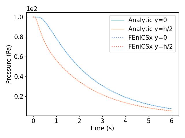
(a)

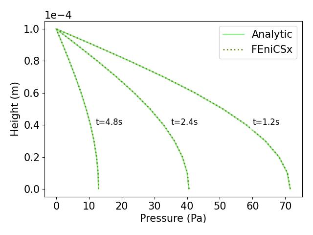
(b)

Figure 2: Comparison of the computed pore pressure against the analytical solution: in (a) time and (b) space. The pressure was well recovered based on the evaluation of the $L^{2}$-norm error $(3.57\pm 2.46)\times 10^{-3}$.

The curves show the efficiency of the simulation to reproduce the analytical solution. The accuracy of the simulation was also supported by the estimation of the error based on the $L^{2}$-norm of the pressure equal to $(3.57\pm 2.46)\times 10^{-3}$ which is deemed satisfactory. The same problem was solved using the legacy FEniCS version. The proposed FEniCSx implementation was faster. It was computed in 9.48 seconds compared to the previously 31.82 seconds.

To show the efficiency of the parallel computation, the 3D case A is considered. For a given spatio-temporal discretization, a larger computational time of 1 hour 4 minutes 29 seconds is needed using FEniCSx. To reduce the time, the code naturally supports parallel computation. The same code was run for several number of threads. Computed on 2 threads, the code required 53 minutes 27 seconds. For 4 threads, the running time was further reduced to 46 minutes 27 seconds. Finally, using 8 threads, the computation time was reduced up to 28 minutes 9 seconds.

Finally, a convergence analysis on the meshing of the column was carried out. The $L_{2}$ error metric was used and its evolution for a $n_{x}\times n_{y}$ discretized mesh is given Figure 3. As we could have expected from the 1D behavior of a confined compression Terzaghi case, the error is almost independent from the $n_{x}$ choice. Figure 3(a) shows that a $n_{y}\geq 10$ gives better estimations. According to Figure 3(b), a balance between precision and computation time must be considered. The more elements, the higher the computation time. To ensure obtaining a reliable solution, a mesh of $n_{x}\times n_{y}=2\times 40$ was used.

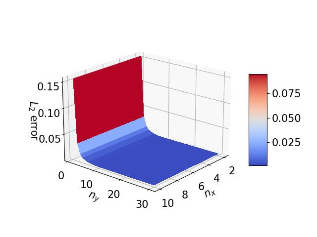
(a)

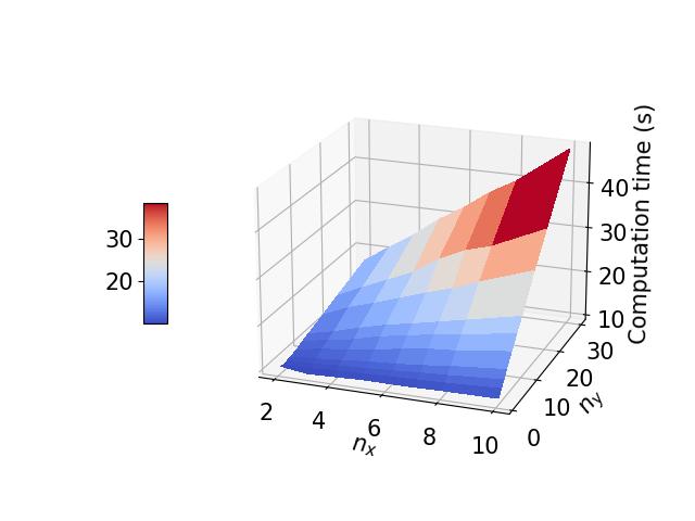
(b)

Figure 3: Convergence analysis for a $n_{x}\times n_{y}$ discretized mesh: L-2 norm (a) and Computation time (b)

3.6 3D hyper-elastic scaffold

3.6.1 FEniCSx implementation

The implementation method of the 3D case is the same. However, special attention must be placed on the boundary. Indeed, moving from 2D to 3D introduces two more boundaries. Therefore, the Dirichlet boundary conditions definition is completed with:

⬇

# uz=0

facets = facet_tag.find(5)

dofs = locate_dofs_topological(MS.sub(0).sub(2), fdim, facets)

bcs.append(dirichletbc(ScalarType(0), dofs, MS.sub(0).sub(2)))

# uz=0

facets = facet_tag.find(6)

dofs = locate_dofs_topological(MS.sub(0).sub(2), fdim, facets)

bcs.append(dirichletbc(ScalarType(0), dofs, MS.sub(0).sub(2)))

The effective stress tensor is also different. As an example, the stress tensor resulting from the potential $W(\mathbf{F})=\tilde{W}_{1}(I_{1},J)+U_{1}(J)$ is defined in FEniCSx by:

⬇

def teff(u,lambda_m,mu):

from ufl import variable, Identity, grad, det, tr, ln, diff

## Deformation gradient

F = variable(Identity(len(u)) + grad(u))

J = variable(det(F))

## Right Cauchy-Green tensor

C = variable(F.T * F)

##Invariants of deformation tensors

Ic = variable(tr(C))

## Potential

W = (mu / 2) * (Ic - 3) - mu * ln(J) + (lambda_m / 2) * (ln(J))**2

return diff(W, F)

All other developed potential are available in the supplementary material.

3.6.2 Results

The same solver options as for the 2D case were used. To limit the computation time, the time step was made variable: dt=500 for $t\in[0,20000]$, dt=1000 for $t\in[20000,60000]$ and dt=10000 for $t\in[60000,100000]$. A total of 84 time steps was then considered.

The parameters were set according to Table 2. The results for the previously defined strain-energy potential are given Figure 4. Each finite element problem was computed in $23.6\pm 4.3$ seconds on 8 threads. Independently from the choice of the potential, the consolidated pressure was retrieved. On the contrary, the resulting displacement depends on the chosen potential but a same order of magnitude is found for all the cases and describe well the observations proposed in Selvadurai and Suvorov [34].

In the absence of information about the porosity or the fluid bulk modulus in the referent study, two fluid bulk modulus were considered. In case where the fluid bulk modulus is made close to the water one ($K^{f}=2.2\times 10^{9}$), the hyper-elastic material well recovers the expected values. However, mismatches appear for a linear scaffold. This can result from the use of a elastic law for large deformations. For example, an Abaqus user would specify the geometric non-linearity whereas no special care was applied in the current example. Furthermore, in case of a lower value of the fluid bulk modulus $K^{f}=5\times 10^{5}$ (i.e., it can correspond to a non-constant value of the permeability and the porosity), the elastic behavior was recovered but differences on the hyper-elastic formulation were obtained.

We believe that these differences result from a permeability depending on the stress state of the column which has not been developed in the referent paper (’Initial values of the permeability and viscosity are the same for all three materials.’ from Selvadurai and Suvorov [34]).

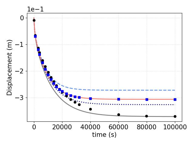
(a)

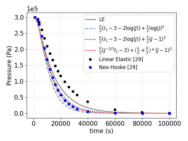
(b)

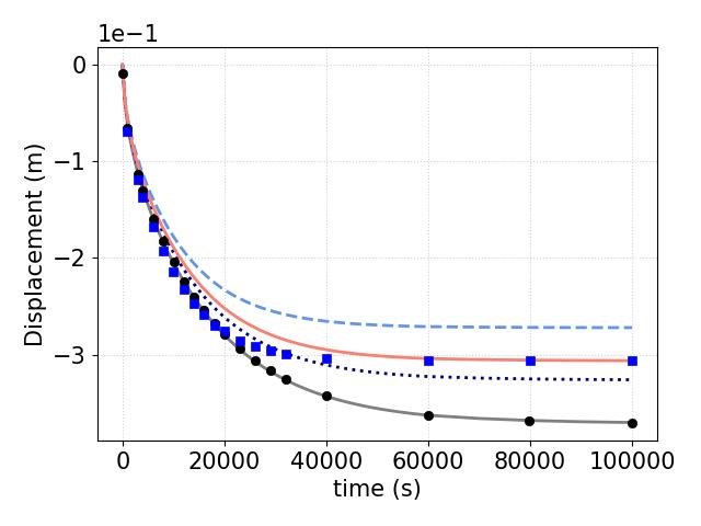
(c)

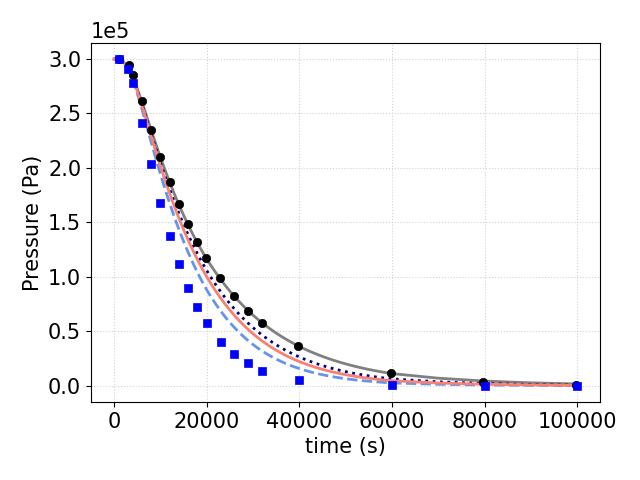
(d)

Figure 4: $K^{f}=2.2\times 10^{9}$: (a) Displacement of the to surface points and (b) pressure at the bottom of the column. $K^{f}=5\times 10^{5}$: (c) Displacement of the to surface points and (d) pressure at the bottom of the column. The computed Linear Elastic (LE) and Neo-Hookean (NH) for both volumetric functions and the found calibrated parameters are super-imposed with the expected values from Selvadurai and Suvorov [34].

4 Confined bi-compartment porous-elastic medium

Sections 3 proposed a poro-mechanical modeling of a single-compartment porous medium (suitable for an avascularised tissue for instance). In case of in vivo modeling, at least one more fluid phase is required: the blood. A 3D confined compression example of a column of height 100 $\mathrm{\SIUnitSymbolMicro m}$ is proposed, based on the here-after variational formulation and Sciumè [7] study. The load is applied as a sinusoidal ramp up to the magnitude of 100 $\mathrm{Pa}$ during 5 seconds. Then, the load is sustained for 125 seconds.

For more complex geometries, a gmsh example of a rectangle geometry indented by a cylindrical beam on its top surface and the corresponding local refinement are proposed B.

Parameter	Symbol	Value	Unit
Young modulus	E	5000	$\mathrm{Pa}$
Poisson ratio	$\nu$	0.2	-
IF viscosity	$\mu^{l}$	1	$\mathrm{Pa}\text{\,}\mathrm{s}$
Intrinsic permeability	$k^{\varepsilon}$	$1.\times 10^{-14}$	${\mathrm{m}}^{2}$
Biot coefficient	$\beta$	1	-
Density of phase $\alpha$	$\rho^{\alpha}$	-	$\mathrm{kg}\text{\,}{\mathrm{m}}^{-3}$
Porosity	$\varepsilon^{l}$	0.5	-
Vessel Bulk modulus	$K^{\nu}$	$1\times 10^{3}$	$\mathrm{Pa}$
vessel Intrinsic permeability	$k^{\varepsilon}_{b}$	$2\times 10^{-16}$ or $4\times 10^{-16}$	${\mathrm{m}}^{2}$
Blood viscosity	$\mu^{b}$	$4.0\times 10^{-3}$	$\mathrm{Pa}\text{\,}\mathrm{s}$
Initial vascular porosity	$\varepsilon^{b}_{0}$	0% or 2% or 4%	-
Vascular porosity	$\varepsilon^{b}$	Equation 48	-

Table 4: Mechanical parameters for the bi-compartment model

4.1 Governing Equations

Let one consider a vascular multi-compartment structure composed of a solid scaffold filled with interstitial fluid (IF) and blood. The medium is assumed saturated. The following convention is assumed: $\bullet^{s}$ denotes the solid phase, $\bullet^{l}$ denotes the interstitial fluid phase (IF) and $\bullet^{b}$ denotes the vascular part. The primary variables of the problem are the pressure applied in the pores of the extra-vascular part of the porous medium, namely $p^{l}$, the blood pressure, namely $p^{b}$, and the displacement of the solid scaffold, namely $\mathbf{u}^{s}$. (Equation 36) links the different volume fractions. The volume fraction of the phase $\alpha$ is defined by (Equation 6). $\varepsilon^{l}$ is called the extra-vascular porosity of the medium.

$$\varepsilon^{s}+\varepsilon^{l}+\varepsilon^{b}=1$$ (36)

Assuming that there is no inter-phase mass transport (i.e. the IF and the blood are assumed pure phases), the continuity equations (mass conservation) of the solid, the IF and the blood phases are respectively given by Equation 37, 38, 39.

$$\frac{\partial}{\partial t}(\rho^{s}(1-\varepsilon^{l}-\varepsilon^{b}))+\nabla\cdot(\rho^{s}(1-\varepsilon^{l}-\varepsilon^{b})\mathbf{v^{s}})=0$$ (37)

$$\frac{\partial}{\partial t}(\rho^{l}\varepsilon^{l})+\nabla\cdot(\rho^{l}\varepsilon^{l}\mathbf{v}^{l})=0$$ (38)

$$\frac{\partial}{\partial t}(\rho^{b}\varepsilon^{b})+\nabla\cdot(\rho^{b}\varepsilon^{b}\mathbf{v}^{b})=0$$ (39)

According to section 3.2, and dividing each equation by the corresponding density, the continuity equations can be re-expressed as:

$$\frac{\mathrm{D}^{s}}{\mathrm{D}t}(1-\varepsilon^{l}-\varepsilon^{b})+(1-\varepsilon^{l}-\varepsilon^{b})\nabla\cdot\mathbf{v^{s}}=0$$ (40)

$$\frac{\mathrm{D}^{s}\varepsilon^{l}}{\mathrm{D}t}+\nabla\cdot(\varepsilon^{l}(\mathbf{v}^{l}-\mathbf{v}^{s}))+\varepsilon^{l}\nabla\cdot\mathbf{v^{s}}=0$$ (41)

$$\frac{\mathrm{D}^{s}\varepsilon^{b}}{\mathrm{D}t}+\nabla\cdot(\varepsilon^{b}(\mathbf{v}^{b}-\mathbf{v}^{s}))+\varepsilon^{b}\nabla\cdot\mathbf{v^{s}}=0$$ (42)

For the fluid phase, Darcy’s law (Equation 43, 44) is used to evaluate the fluid flow in the porous medium.

$$\varepsilon^{l}(\mathbf{v}^{l}-\mathbf{v}^{s})=-\frac{k^{\varepsilon}}{\mu^{l}}(\mathbf{\nabla}p^{l}-\rho^{l}\mathbf{g})$$ (43)

$$\varepsilon^{b}(\mathbf{v}^{b}-\mathbf{v}^{s})=-\frac{k^{b}}{\mu^{b}}(\mathbf{\nabla}p^{b}-\rho^{b}\mathbf{g})$$ (44)

Where $k^{\varepsilon}$, $k^{b}$ are the intrinsic permeabilities (${\mathrm{m}}^{2}$), $\mu^{l}$, $\mu^{b}$ are the dynamic viscosities ($\mathrm{Pa}\text{\,}\mathrm{s}$), $p^{l}$, $p^{b}$ the pressures and $\mathbf{g}$ the gravity.

Equation 39 gives the following relationship:

$$\frac{\mathrm{D}^{s}\varepsilon^{l}}{\mathrm{D}t}=-\frac{\mathrm{D}^{s}\varepsilon^{b}}{\mathrm{D}t}+(1-\varepsilon^{l}-\varepsilon^{b})\nabla\cdot\mathbf{v^{s}}$$ (45)

Considering Equations 43, 45, Equation 41 becomes:

$$-\frac{\mathrm{D}^{s}\varepsilon^{b}}{\mathrm{D}t}-\nabla\cdot(\frac{k^{\varepsilon}}{\mu^{l}}\mathbf{\nabla}p^{l})+(1-\varepsilon^{b})\nabla\cdot\mathbf{v^{s}}=0$$ (46)

Then, reading Equation 44, Equation 42 gives:

$$\frac{\mathrm{D}^{s}\varepsilon^{b}}{\mathrm{D}t}-\nabla\cdot(\frac{k^{b}}{\mu^{b}}\mathbf{\nabla}p^{b})+\varepsilon^{b}\nabla\cdot\mathbf{v^{s}}=0$$ (47)

Considering a vascular tissue, we assume that the blood vessels are mostly surrounded by IF so they have weak direct interaction with the solid scaffold. Furthermore, the vessels are assumed compressible. Therefore, a state equation for the volume fraction of blood is introduced Equation 48.

$$\varepsilon^{b}=\varepsilon^{b}_{0}\cdot\left(1-\frac{p^{l}-p^{b}}{K^{\nu}}\right)$$ (48)

Where $\varepsilon^{b}_{0}$ denotes the blood volume fraction when $p^{l}=p^{b}$, $K^{\nu}$ is the vessel compressibility.

It follows that Equations 46, 47 can be re-written as:

$$-\frac{\varepsilon^{b}_{0}}{K^{\nu}}\left(\frac{\mathrm{D}^{s}p^{l}}{\mathrm{D}t}-\frac{\mathrm{D}^{s}p^{b}}{\mathrm{D}t}\right)-\nabla\cdot(\frac{k^{\varepsilon}}{\mu^{l}}\mathbf{\nabla}p^{l})+(1-\varepsilon^{b})\nabla\cdot\mathbf{v^{s}}=0$$ (49)

$$\frac{\varepsilon^{b}_{0}}{K^{\nu}}\left(\frac{\mathrm{D}^{s}p^{l}}{\mathrm{D}t}-\frac{\mathrm{D}^{s}p^{b}}{\mathrm{D}t}\right)-\nabla\cdot(\frac{k^{b}}{\mu^{b}}\mathbf{\nabla}p^{b})+\varepsilon^{b}\nabla\cdot\mathbf{v^{s}}=0$$ (50)

Once the continuity equations are settled, one can define the quasi-static momentum balance of the porous medium, Equation 51.

$$\mathbf{\nabla}\cdot\mathbf{t}^{\text{tot}}=0$$ (51)

Where $\mathbf{t}^{\text{tot}}$ is the total Cauchy stress tensor. We introduce an effective stress tensor denoted $\mathbf{t}^{\text{eff}}$, responsible for all deformation of the solid scaffold. Then, $\mathbf{t}^{\text{tot}}$ can be expressed as:

$$\mathbf{t}^{tot}=\mathbf{t}^{\text{eff}}-(1-\zeta)p^{l}\mathbf{I_{d}}-\zeta p^{b}\mathbf{I_{d}}$$ (52)

$$\mathbf{\epsilon}(\mathbf{u})=\frac{1}{2}(\nabla\mathbf{u}+\nabla\mathbf{u}^{\text{T}})$$ (53)

$$\mathbf{t}^{\text{eff}}=2\mu\mathbf{\epsilon}(\mathbf{u}^{s})+\lambda\text{tr}(\mathbf{\epsilon}(\mathbf{u}^{s}))\mathbf{I_{d}}$$ (54)

$$\zeta=\varepsilon_{0}^{b}\left(1-2\frac{p^{l}-p^{b}}{K^{\nu}}\right)$$ (55)

Four boundaries are defined: the first one, $\Gamma_{u}$ has imposed displacement (Equation 56), the second one $\Gamma_{s}$ has imposed external forces (Equation 57) and $\Omega_{p}$ has imposed pressure (fluid leakage condition (Equation 58, 59)). We obtain:

$$\mathbf{t}^{\text{eff}}=\mathbf{t}^{\text{imposed}}~{}\text{on}~{}\Gamma_{s}$$ (56)

$$\mathbf{u}^{s}=\mathbf{u}^{\text{imposed}}~{}\text{on}~{}\Gamma_{u}$$ (57)

$$p^{l}=0~{}\text{on}~{}\Gamma_{p}$$ (58)

$$p^{b}=0~{}\text{on}~{}\Gamma_{p}$$ (59)

The initial conditions are given Table 5.

Parameter	Symbol	Value	Unit
Displacement	$\mathbf{u}^{s}$	0	$\mathrm{m}$
Displacement at previous step	$\mathbf{u}^{s}_{n}$	0	$\mathrm{m}$
IF pressure	$p^{l}$	0	$\mathrm{Pa}$
IF pressure at previous step	$p^{l}_{n}$	0	$\mathrm{Pa}$
Blood pressure	$p^{b}$	0	$\mathrm{Pa}$
Blood pressure at previous time step	$p^{b}$	0	$\mathrm{Pa}$
Vascular porosity	$\varepsilon^{b}$	$\varepsilon^{b}_{0}$	-

Table 5: Initial conditions for the bi-compartment model

4.2 Variational Form

For the computation of the FE model, the variational form of Equation 49-51 must be introduced. Let one consider ($q^{l}$,$q^{b}$,v) the test functions defined in the mixed space $\text{L}_{0}^{2}(\Omega)\times\text{L}_{0}^{2}(\Omega)\times[\text{H}^{1}(\Omega)]^{3}$. With a first order approximation in time, Equation 49, 50 gives:

$$\begin{split}-\frac{\varepsilon^{b}_{0}}{K^{\nu}}\frac{1}{dt}\int_{\Omega}(p^{b}-p^{b}_{n}-p^{l}+p^{l}_{n})q^{l}\text{d}\Omega+\frac{1-\varepsilon^{b}}{dt}\int_{\Omega}\mathbf{\nabla}\cdot(\mathbf{u}^{s}-\mathbf{u}^{s}_{n})q^{l}\text{d}\Omega\\ +\frac{k^{\varepsilon}}{\mu^{l}}\int_{\Omega}\mathbf{\nabla}p^{l}\mathbf{\nabla}q^{l}\text{d}\Omega=0,\forall~{}q^{l}\in~{}\text{L}_{0}^{2}(\Omega)\end{split}$$ (60)

$$\begin{split}\frac{\varepsilon^{b}}{K^{\nu}}\frac{1}{dt}\int_{\Omega}(p^{b}-p^{b}_{n}-p^{l}+p^{l}_{n})q^{b}\text{d}\Omega+\frac{\varepsilon^{b}}{dt}\int_{\Omega}\mathbf{\nabla}\cdot(\mathbf{u}^{s}-\mathbf{u}^{s}_{n})q^{b}\text{d}\Omega\\ +\frac{k^{b}}{\mu^{b}}\int_{\Omega}\mathbf{\nabla}p^{b}\mathbf{\nabla}q^{b}\text{d}\Omega=0,\forall~{}q^{b}\in~{}\text{L}_{0}^{2}(\Omega)\end{split}$$ (61)

Similarly, by integrating by part Equation 51, and including the Neumann boundary conditions, we get:

$$\begin{split}\int_{\Omega}\mathbf{t}^{\text{eff}}:\mathbf{\nabla}\mathbf{v}\text{d}\Omega-\int_{\Omega}(1-\zeta)p^{l}\mathbf{\nabla}\cdot\mathbf{v}\text{d}\Omega\\ -\int_{\Omega}\zeta p^{b}\mathbf{\nabla}\cdot\mathbf{v}\text{d}\Omega\\ -\int_{\Gamma_{s}}\mathbf{t}^{\text{imposed}}\cdot\mathbf{v}\text{d}\Gamma_{s}=0,\forall~{}v\in~{}[\text{H}^{1}(\Omega)]^{3}\end{split}$$ (62)

4.3 FEniCSx Implementation

This section provides the code of a multi-compartment 3D column in confined compression. In order to evaluate the FEniCSx implementation, this case is similar to the Cast3m solution proposed in Sciumè [7]. 3 cases are studied: avascular tissue, vascular porosity of 2% and vascular porosity of 4%. The load is applied as a sine ramp during 5 seconds and then sustained during 125 seconds.

The time discretization is introduced.

⬇

t, t_ramp, t_sust = 0, 5, 125 # Start time

Tf = t_ramp+t_sust # End time

num_steps = 1301 # Number of time steps

dt = (Tf-t)/num_steps # Time step size

We then introduce the material parameters according to Table 5. The three cases of vascularization and Equation 55 are defined.

⬇

E = Constant(mesh, ScalarType(5000))

nu = Constant(mesh, ScalarType(0.2))

kepsilon_l = Constant(mesh, ScalarType(1e-14))

mu_l = Constant(mesh, ScalarType(1))

lambda_m = Constant(mesh, ScalarType(E.value*nu.value/((1+nu.value)*(1-2*nu.value))))

mu = Constant(mesh, ScalarType(E.value/(2*(1+nu.value))))

Knu = Constant(mesh, ScalarType(1000)) #compressibility of the vessels

mu_b = Constant(mesh, ScalarType(0.004)) #dynamic mu_l of the blood

case=1

if case ==0:

epsilon_b_0=Constant(mesh, ScalarType(0.00)) #initial vascular porosity

k_b=Constant(mesh, ScalarType(2e-16)) #intrinsic permeability of vessels

def zeta(pl,pb):

return Constant(mesh,ScalarType(0.))

elif case ==1:

epsilon_b_0=Constant(mesh, ScalarType(0.02)) #initial vascular porosity

k_b=Constant(mesh, ScalarType(2e-16)) #intrinsic permeability of vessels

def zeta(pl,pb):

return epsilon_b_0.value*(1-2*(pl-pb)/Knu.value)

elif case ==2:

epsilon_b_0 = Constant(mesh, ScalarType(0.04)) #initial vascular porosity

k_b = Constant(mesh, ScalarType(4e-16)) #intrinsic permeability of vessels

def zeta(pl,pb):

return epsilon_b_0.value*(1-2*(pl-pb)/Knu.value)

Then, the integration space, boundary and initial conditions are set up for the displacement, the IF pressure and the blood pressure.

⬇

## Mechanical loading (Terzaghi)

pinit = 200 #[Pa]

T = Constant(mesh,ScalarType(-pinit))

## Define Mixed Space (R2,R, R) -> (u,pl, pb)

element = VectorElement("CG", mesh.ufl_cell(), 2)

pressure_element = FiniteElement("CG", mesh.ufl_cell(), 1)

MS = FunctionSpace(mesh, MixedElement([element,pressure_element,pressure_element]))

# Create the solution and initial spaces

X0 = Function(MS)

Xn = Function(MS)

# Create the surfacic element

ds = Measure("ds", domain=mesh, subdomain_data=facet_tag)

# compute the normals

normal = FacetNormal(mesh)

# Define the Dirichlet conditions

bcs = []

# uy=0

facets = facet_tag.find(1)

dofs = locate_dofs_topological(MS.sub(0).sub(1), fdim, facets)

bcs.append(dirichletbc(ScalarType(0), dofs, MS.sub(0).sub(1)))

# ux=0

facets = facet_tag.find(2)

dofs = locate_dofs_topological(MS.sub(0).sub(0), fdim, facets)

bcs.append(dirichletbc(ScalarType(0), dofs, MS.sub(0).sub(0)))

# ux=0

facets = facet_tag.find(4)

dofs = locate_dofs_topological(MS.sub(0).sub(0), fdim, facets)

bcs.append(dirichletbc(ScalarType(0), dofs, MS.sub(0).sub(0)))

# uz=0

facets = facet_tag.find(5)

dofs = locate_dofs_topological(MS.sub(0).sub(2), fdim, facets)

bcs.append(dirichletbc(ScalarType(0), dofs, MS.sub(0).sub(2)))

# uz=0

facets = facet_tag.find(6)

dofs = locate_dofs_topological(MS.sub(0).sub(2), fdim, facets)

bcs.append(dirichletbc(ScalarType(0), dofs, MS.sub(0).sub(2)))

# leakage pl=pb=0

facets = facet_tag.find(3)

dofs = locate_dofs_topological(MS.sub(1), fdim, facets)

bcs.append(dirichletbc(ScalarType(0), dofs, MS.sub(1)))

dofs = locate_dofs_topological(MS.sub(2), fdim, facets)

bcs.append(dirichletbc(ScalarType(0), dofs, MS.sub(2)))

# Set Initial values

# Displacement

Un_, Un_to_MS = MS.sub(0).collapse()

FUn_ = Function(Un_)

with FUn_.vector.localForm() as initial_local:

initial_local.set(ScalarType(0.0))

# Update Xn for all threads

Xn.x.array[Un_to_MS] = FUn_.x.array

Xn.x.scatter_forward()

# IF Pressure

Pn_, Pn_to_MS = MS.sub(1).collapse()

FPn_ = Function(Pn_)

with FPn_.vector.localForm() as initial_local:

initial_local.set(ScalarType(0))

# Update Xn for all threads

Xn.x.array[Pn_to_MS] = FPn_.x.array

Xn.x.scatter_forward()

# Blood Pressure

Pbn_, Pbn_to_MS = MS.sub(2).collapse()

FPbn_ = Function(Pbn_)

with FPbn_.vector.localForm() as initial_local:

initial_local.set(ScalarType(0))

# Update Xn for all threads

Xn.x.array[Pbn_to_MS] = FPbn_.x.array

Xn.x.scatter_forward()

Internal variables are required. The vessels are compressible so we include the evolution of the vascular porosity as a function representing Equation 48.

⬇

# Internal variables: vascular porosity

Poro_space = FunctionSpace(mesh,pressure_element)

poro_b = Function(Poro_space) # vascular porosity

# Initialize

with poro_b.vector.localForm() as initial_local:

initial_local.set(ScalarType(epsilon_b_0.value))

# Update

poro_b.x.scatter_forward()

poro_b.name="poro_b"

A xdmf file is opened to store the results.

⬇

xdmf = XDMFFile(mesh.comm, "terzaghi.xdmf", "w")

xdmf.write_mesh(mesh)

The test functions as well as the variational form are introduced according to Equations 60, 61, 62.

⬇

u, pl, pb = split(X0)

u_n, pl_n, pb_n = split(Xn)

v, ql, qb = TestFunctions(MS)

dx = Measure("dx", metadata={"quadrature_degree": 4})

F = (1-poro_b)*(1/dt)*nabla_div(u-u_n)*ql*dx + ( kepsilon_l/(mu_l) )*dot( grad(pl),grad(ql) )*dx - (epsilon_b_0/Knu)*( (1/dt)*(pb-pb_n-pl+pl_n) )*ql*dx

F += poro_b*(1/dt)*nabla_div(u-u_n)*qb*dx + ( k_b/(mu_b) )*dot( grad(pb),grad(qb) )*dx + (epsilon_b_0/Knu)*( (1/dt)*(pb-pb_n-pl+pl_n) )*qb*dx

F += inner(grad(v),teff(u))*dx - (1-zeta(pl,pb))*pl*nabla_div(v)*dx - zeta(pl,pb)*pb*nabla_div(v)*dx - T*inner(v,normal)*ds(3)

Finally, the problem to be solved is defined and a Newton method is used for each time step, the vascular porosity is updated and the results are stored in the xdmf file.

⬇

dX0 = TrialFunction(MS)

J = derivative(F, X0, dX0)

Problem = NonlinearProblem(F, X0, bcs = bcs, J = J)

solver = nls.petsc.NewtonSolver(mesh.comm, Problem)

# Set Newton solver options

solver.atol = 5e-10

solver.rtol = 1e-11

solver.convergence_criterion = "incremental"

t = 0

for n in range(num_steps):

t += dt

if t < t_ramp:

f1 = 0.5 * (1 - np.cos(np.pi*t/t_ramp))

else:

f1 = 1

T.value = -200*f1

num_its, converged = solver.solve(X0)

X0.x.scatter_forward()

# Update Value

Xn.x.array[:] = X0.x.array

Xn.x.scatter_forward()

# Update porosity

poro_b.x.array[:] = epsilon_b_0.value*(1-(1/Knu.value)*(X0.x.array[Pn_to_MS]-X0.x.array[Pbn_to_MS]))

poro_b.x.scatter_forward()

# Save data

__u, __pl, __pb = X0.split()

__u.name = "Displacement"

__pl.name = "Pressure IF"

__pb.name = "Pressure blood"

xdmf.write_function(__u,t)

xdmf.write_function(__pl,t)

xdmf.write_function(__pb,t)

xdmf.write_function(poro_b,t)

xdmf.close()

4.4 Results

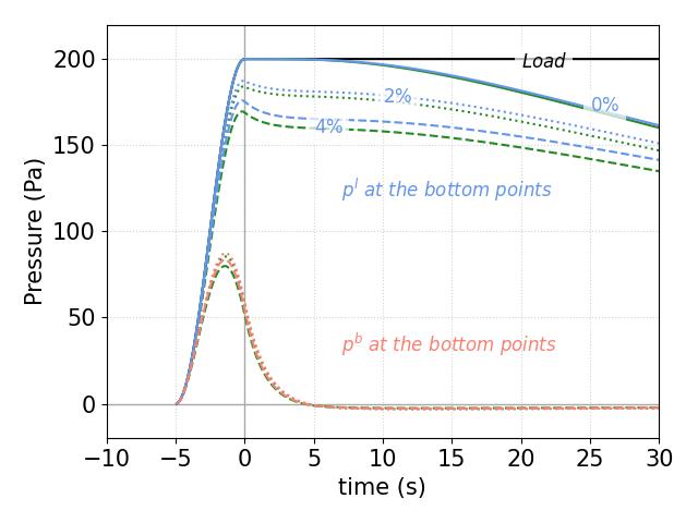
(a)

(b)

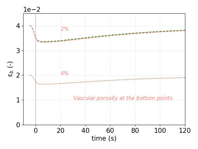
(c)

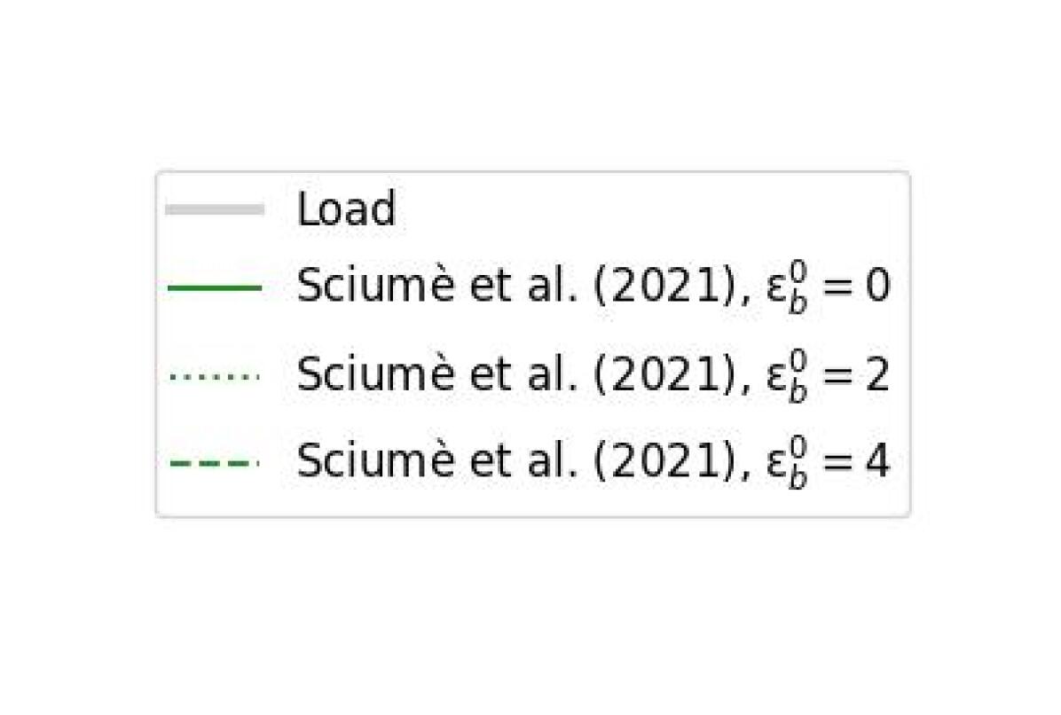
Figure 5: Comparison of the results obtained using FEniCSx against Sciumè [7] results. All results were shifted to obtain similar figures. The solid, doted and dashed lines respectively represent the 0%, 2% 4% initial vascular porosity. (a) Evolution of the pressure at the bottom points. (b) Displacement of the top points. (c) Vascular porosity at the bottom points. The behavior was well retrieved for all the cases with a NRMSE lower than 10% for all variables according to Table 6.

The evolution of the vascular and interstitial pressures at the bottom points and the vertical displacement at the top points are provided Figure 5. Each solution was obtained in $6\pm 2$ minutes on 8 threads. The overall behavior of the interstitial fluid pressure, the blood pressure and the solid displacement were retrieved. To quantitatively assess the reliability of our implemented model, The normalized root mean square error (NRMSE, Equation 63) was computed for each case with the results obtained with Cast3m in Sciumè [7], Table 6.

$$\text{NRMSE}(x,x^{\text{ref}})=\frac{\sqrt{\frac{1}{N}\sum_{i\in[1,N]}(x-x^{\text{ref}})^{2}}}{\text{mean}(x^{\text{ref}})}$$ (63)

Parameter	0%	2%	4%
$p^{l}$	1.4 $\mathrm{\char 37\relax}$	3.1 $\mathrm{\char 37\relax}$	5.1 $\mathrm{\char 37\relax}$
$u_{y}$	0.3 $\mathrm{\char 37\relax}$	2.2 $\mathrm{\char 37\relax}$	3.7 $\mathrm{\char 37\relax}$
$p^{b}$	-	4.7 $\mathrm{\char 37\relax}$	8.8 $\mathrm{\char 37\relax}$
$\varepsilon^{b}_{0}$	-	0.4 $\mathrm{\char 37\relax}$	0.6 $\mathrm{\char 37\relax}$

Table 6: NRMSE computed for each studied variable.

The NRMSE was found lower than 10% for all unknowns. The differences are assumed to result from the method of resolution which differs between Cast3m and FEniCSx. Indeed, the Cast3m procedure relies on a staggered solver whereas our results were obtained using a monolithic solver. The order of magnitudes of the NRMSE made us however consider our solution as trustworthy.

5 Conclusion

The objective of this paper was to propose a step-by-step explanation of how to implement several poro-mechanical models in FEniCSx with special attention to parallel computation. Several benchmark cases for a mixed formulation were evaluated. First, a confined column was simulated under compression. Accurate results according to the L2-norm were found compared to the analytical solution. Furthermore, the code was computed 3 times faster than in the legacy FEniCS environment. Then, a possible implementation of a hyper-elastic formulation was proposed. The model was validated using Selvadurai and Suvorov [34] values. Finally, a confined bi-compartment sample was simulated. The results were compared to Sciumè [7] data. Small differences were observed due to the choice of the solver (staggered or monolithic) but remained acceptable. The authors hope that this paper will contribute to facilitate the use of poro-elasticity in the biomechanical engineering community. This article and its supplementary material constitute a starting point to implement their own material models at a preferred level of complexity.

6 Supplementary material

The python codes corresponding to the workflows and the docker file of this article are made available for 2D and 3D cases on the following link: https://github.com/Th0masLavigne/Dolfinx_Porous_Media.git.

7 Declaration of Competing Interest

Authors have no conflicts of interest to report.

8 Acknowledgment

This research was funded in whole, or in part, by the Luxembourg National Research Fund (FNR),grant reference No. 17013182. For the purpose of open access, the author has applied a Creative Commons Attribution 4.0 International (CC BY 4.0) license to any Author Accepted Manuscript version arising from this submission. The present project is also supported by the National Research Fund, Luxembourg, under grant No. C20/MS/14782078/QuaC.

Appendix A 3D Terzaghi example

Here-after is proposed a minimal working code corresponding to the 2D case included within the text.

⬇

import numpy as np

import csv

from petsc4py import PETSc

import dolfinx

from dolfinx import nls

from dolfinx.io import XDMFFile

from dolfinx.mesh import CellType, create_box, locate_entities_boundary, locate_entities, meshtags

from dolfinx.fem import (Constant, dirichletbc, Function, FunctionSpace, locate_dofs_topological, form, assemble_scalar)

from dolfinx.fem.petsc import NonlinearProblem

from dolfinx.geometry import BoundingBoxTree, compute_collisions, compute_colliding_cells

from petsc4py.PETSc import ScalarType

from mpi4py import MPI

from ufl import (FacetNormal, Identity, Measure, TestFunctions, TrialFunction, VectorElement, FiniteElement, dot, dx, inner, grad, nabla_div, div, sym, MixedElement, derivative, split)

#

def epsilon(u):

return sym(grad(u))

#

def teff(u):

return lambda_m * nabla_div(u) * Identity(u.geometric_dimension()) + 2*mu*epsilon(u)

#

kmax=1e3

def terzaghi_p(x):

p0,L=pinit,Height

cv = permeability.value/viscosity.value*(lambda_m.value+2*mu.value)

pression=0

for k in range(1,int(kmax)):

pression+=p0*4/np.pi*(-1)**(k-1)/(2*k-1)*np.cos((2*k-1)*0.5*np.pi*(x[1]/L))*np.exp(-(2*k-1)**2*0.25*np.pi**2*cv*t/L**2)

pl=pression

return pl

#

def L2_error_p(mesh,pressure_element,__p):

V2 = FunctionSpace(mesh, pressure_element)

pex = Function(V2)

pex.interpolate(terzaghi_p)

L2_errorp, L2_normp = form(inner(__p - pex, __p - pex) * dx), form(inner(pex, pex) * dx)

error_localp = assemble_scalar(L2_errorp)/assemble_scalar(L2_normp)

error_L2p = np.sqrt(mesh.comm.allreduce(error_localp, op=MPI.SUM))

return error_L2p

#

## Create the domain / mesh

Height = 1e-4 #[m]

Width = 1e-5 #[m]

Length = 1e-5 #[m]

mesh = create_box(MPI.COMM_WORLD, np.array([[0.0,0.0,0.0],[Length, Width, Height]]), [8, 8, 20], cell_type=CellType.tetrahedron)

#

## Define the boundaries:

# 1 = bottom, 2 = right, 3=top, 4=left, 5=back, 6=front

boundaries = [(1, lambda x: np.isclose(x[2], 0)),

(2, lambda x: np.isclose(x[0], Length)),

(3, lambda x: np.isclose(x[2], Height)),

(4, lambda x: np.isclose(x[0], 0)),

(5, lambda x: np.isclose(x[1], Width)),

(6, lambda x: np.isclose(x[1], 0))]

#

facet_indices, facet_markers = [], []

fdim = mesh.topology.dim - 1

for (marker, locator) in boundaries:

facets = locate_entities(mesh, fdim, locator)

facet_indices.append(facets)

facet_markers.append(np.full_like(facets, marker))

facet_indices = np.hstack(facet_indices).astype(np.int32)

facet_markers = np.hstack(facet_markers).astype(np.int32)

sorted_facets = np.argsort(facet_indices)

facet_tag = meshtags(mesh, fdim, facet_indices[sorted_facets], facet_markers[sorted_facets])

#

## Time parametrization

t = 0 # Start time

Tf = 6 # End time

num_steps = 1000 # Number of time steps

dt = (Tf-t)/num_steps # Time step size

#

## Material parameters

E = Constant(mesh, ScalarType(5000))

nu = Constant(mesh, ScalarType(0.4))

lambda_m = Constant(mesh, ScalarType(E.value*nu.value/((1+nu.value)*(1-2*nu.value))))

mu = Constant(mesh, ScalarType(E.value/(2*(1+nu.value))))

rhos = Constant(mesh, ScalarType(1))

permeability = Constant(mesh, ScalarType(1.8e-15))

viscosity = Constant(mesh, ScalarType(1e-2))

rhol = Constant(mesh, ScalarType(1))

beta = Constant(mesh, ScalarType(1))

porosity = Constant(mesh, ScalarType(0.2))

Kf = Constant(mesh, ScalarType(2.2e9))

Ks = Constant(mesh, ScalarType(1e10))

S = (porosity/Kf)+(1-porosity)/Ks

#

## Mechanical loading

pinit = 100 #[Pa]

T = Constant(mesh,ScalarType(-pinit))

#

# Create the surfacic element

ds = Measure("ds", domain=mesh, subdomain_data=facet_tag)

normal = FacetNormal(mesh)

#

# Define Mixed Space (R2,R) -> (u,p)

displacement_element = VectorElement("CG", mesh.ufl_cell(), 2)

pressure_element = FiniteElement("CG", mesh.ufl_cell(), 1)

MS = FunctionSpace(mesh, MixedElement([displacement_element,pressure_element]))

#

# Define the Dirichlet condition

# 1 = bottom: uy=0, 2 = right: ux=0, 3=top: pl=0 drainage, 4=left: ux=0

bcs = []

# uz=0

facets = facet_tag.find(1)

dofs = locate_dofs_topological(MS.sub(0).sub(2), fdim, facets)

bcs.append(dirichletbc(ScalarType(0), dofs, MS.sub(0).sub(2)))

# ux=0

facets = facet_tag.find(2)

dofs = locate_dofs_topological(MS.sub(0).sub(0), fdim, facets)

bcs.append(dirichletbc(ScalarType(0), dofs, MS.sub(0).sub(0)))

# ux=0

facets = facet_tag.find(4)

dofs = locate_dofs_topological(MS.sub(0).sub(0), fdim, facets)

bcs.append(dirichletbc(ScalarType(0), dofs, MS.sub(0).sub(0)))

# uy=0

facets = facet_tag.find(5)

dofs = locate_dofs_topological(MS.sub(0).sub(1), fdim, facets)

bcs.append(dirichletbc(ScalarType(0), dofs, MS.sub(0).sub(1)))

# uy=0

facets = facet_tag.find(6)

dofs = locate_dofs_topological(MS.sub(0).sub(1), fdim, facets)

bcs.append(dirichletbc(ScalarType(0), dofs, MS.sub(0).sub(1)))

# drainage p=0

facets = facet_tag.find(3)

dofs = locate_dofs_topological(MS.sub(1), fdim, facets)

bcs.append(dirichletbc(ScalarType(0), dofs, MS.sub(1)))

#

# Create the initial and solution spaces

X0 = Function(MS)

Xn = Function(MS)

#

# Initial values

#

Un_, Un_to_MS = MS.sub(0).collapse()

FUn_ = Function(Un_)

with FUn_.vector.localForm() as initial_local:

initial_local.set(ScalarType(0.0))

#

# Update Xn

Xn.x.array[Un_to_MS] = FUn_.x.array

Xn.x.scatter_forward()

#

Pn_, Pn_to_MS = MS.sub(1).collapse()

FPn_ = Function(Pn_)

with FPn_.vector.localForm() as initial_local:

initial_local.set(ScalarType(pinit))

#

# Update Xn

Xn.x.array[Pn_to_MS] = FPn_.x.array

Xn.x.scatter_forward()

#

# Variational form

# Identify the unknowns from the function

u,p =split(X0)

u_n,p_n=split(Xn)

# Set up the test functions

v,q = TestFunctions(MS)

# Equation 17

F = (1/dt)*nabla_div(u-u_n)*q*dx + (permeability/viscosity)*dot(grad(p),grad(q))*dx + ( S/dt )*(p-p_n)*q*dx

# Equation 18

F += inner(grad(v),teff(u))*dx - beta * p * nabla_div(v)*dx - T*inner(v,normal)*ds(3)

# Non linear problem definition

dX0 = TrialFunction(MS)

J = derivative(F, X0, dX0)

Problem = NonlinearProblem(F, X0, bcs = bcs, J = J)

# set up the non-linear solver

solver = nls.petsc.NewtonSolver(mesh.comm, Problem)

# Absolute tolerance

solver.atol = 5e-10

# relative tolerance

solver.rtol = 1e-11

solver.convergence_criterion = "incremental"

#

t = 0

L2_p = np.zeros(num_steps, dtype=PETSc.ScalarType)

for n in range(num_steps):

t += dt

num_its, converged = solver.solve(X0)

X0.x.scatter_forward()

# Update Value

Xn.x.array[:] = X0.x.array

Xn.x.scatter_forward()

__u, __p = X0.split()

# Compute L2 norm for pressure

error_L2p = L2_error_p(mesh,pressure_element,__p)

L2_p[n] = error_L2p

# Solve tracking

if mesh.comm.rank == 0:

print(f"Time step {n}, Number of iterations {num_its}, Load {T.value}, L2-error p {error_L2p:.2e}")

if mesh.comm.rank == 0:

print(f"L2 error p, min {np.min(L2_p):.2e}, mean {np.mean(L2_p):.2e}, max {np.max(L2_p):.2e}, std {np.std(L2_p):.2e}")

Appendix B Local refinement

A 3D geometry can be meshed using the GMSH API of python (Geuzaine and Remacle [33]). This allows to represent complex geometries including circle arcs. An optimized and locally refined mesh can be therefore obtained. This example uses the method proposed in the FEniCS project tutorial provided by J. Dokken and G. Wells. An alternative procedure in the FEniCSx environment with local refinement is then proposed in B.2.

B.1 Meshing using GMSH API

First, the environment is initialized and the physical variables required for the box/cylinder creation are defined.

⬇

import gmsh

import numpy as np

#

gmsh.initialize()

#

# box parameters

[Length, Width, Height] = [6e-4, 2.5e-4, 4e-5]

# cylinder parameters

xc,yc,zc,dx,dy,dz, r = 6e-4/2, 0, 0, 0, 0, 4e-5, 1.5e-4

# expected dimension of the mesh

gdim = 3

The geometries are created using built-in functions of GMSH; potential duplicates are removed.

⬇

# create the geometry

box = gmsh.model.occ.addBox(0, 0, 0, Length, Width, Height)

cylinder = gmsh.model.occ.addCylinder(xc,yc,zc,dx,dy,dz, r,tag=1000,angle=np.pi)

gmsh.model.occ.synchronize()

# Remove duplicate entities and synchronize

gmsh.model.occ.removeAllDuplicates()

gmsh.model.occ.synchronize()

Physical groups are defined: the volumes for the 3D meshing and the surfaces for tagging. Surface groups were identified based on the coordinates of the center of mass of each surface.

⬇

surfaces, volumes = [gmsh.model.getEntities(d) for d in [ gdim-1, gdim]]

print(volumes)

# Volumes

gmsh.model.addPhysicalGroup(volumes[0][0], [volumes[0][1]], -1)

gmsh.model.setPhysicalName(volumes[0][0], -1, ’Half_Cylinder’)

gmsh.model.addPhysicalGroup(volumes[1][0], [volumes[1][1]], -1)

gmsh.model.setPhysicalName(volumes[1][0], -1, ’Box’)

# 1 = loading, 2 = top minus loading, 3 = bottom, 4 = left, 5 = right, 6 = Front, 7 = back

bottom_marker, front_marker, back_marker, left_marker, right_marker, top_marker, indenter_marker = 3, 6, 7, 4, 5, 2, 1

bottom, front, back, left, right, top, indenter = [],[],[],[],[],[],[]

boundaries = gmsh.model.getBoundary(volumes, oriented=False)

for boundary in boundaries:

center_of_mass = gmsh.model.occ.getCenterOfMass(boundary[0], boundary[1])

if np.isclose(center_of_mass[1], Width):

back.append(boundary[1])

elif np.isclose(center_of_mass[1], 0):

front.append(boundary[1])

elif np.isclose(center_of_mass[0], 0):

left.append(boundary[1])

elif np.isclose(center_of_mass[0], Length):

right.append(boundary[1])

elif np.isclose(center_of_mass[2], 0):

bottom.append(boundary[1])

elif np.isclose(center_of_mass[2], Height) and center_of_mass[1]>Width/3:

top.append(boundary[1])

else:

indenter.append(boundary[1])

# mark the surfaces

gmsh.model.addPhysicalGroup(boundaries[0][0], bottom, bottom_marker)

gmsh.model.setPhysicalName(boundaries[0][0], bottom_marker, ’bottom’)

gmsh.model.addPhysicalGroup(boundaries[0][0], front, front_marker)

gmsh.model.setPhysicalName(boundaries[0][0], front_marker, ’front’)

gmsh.model.addPhysicalGroup(boundaries[0][0], back, back_marker)

gmsh.model.setPhysicalName(boundaries[0][0], back_marker, ’back’)

gmsh.model.addPhysicalGroup(boundaries[0][0], left, left_marker)

gmsh.model.setPhysicalName(boundaries[0][0], left_marker, ’left’)

gmsh.model.addPhysicalGroup(boundaries[0][0], right, right_marker)

gmsh.model.setPhysicalName(boundaries[0][0], right_marker, ’right’)

gmsh.model.addPhysicalGroup(boundaries[0][0], top, top_marker)

gmsh.model.setPhysicalName(boundaries[0][0], top_marker, ’top’)

gmsh.model.addPhysicalGroup(boundaries[0][0], indenter, indenter_marker)

gmsh.model.setPhysicalName(boundaries[0][0], indenter_marker, ’indenter’)

gmsh.model.occ.synchronize()

# Write a geo file for verification in the GMSH GUI

gmsh.write(’Geom_2reelle_8EP.geo_unrolled’)

Then, a threshold function is defined over a distance field to mesh the circular area. This allows for creating an adaptive mesh: coarse far from the circular area, refine close to it.

⬇

indenter_interface = surfaces[0][1]

distance = gmsh.model.mesh.field.add("Distance")

gmsh.model.mesh.field.setNumbers(distance, "FacesList", [indenter_interface])

# A threshold function is defined:

resolution = r/10

threshold = gmsh.model.mesh.field.add("Threshold")

gmsh.model.mesh.field.setNumber(threshold, "IField", distance)

gmsh.model.mesh.field.setNumber(threshold, "LcMin", resolution)

gmsh.model.mesh.field.setNumber(threshold, "LcMax", 5*resolution)

gmsh.model.mesh.field.setNumber(threshold, "DistMin", 0.6*r)

gmsh.model.mesh.field.setNumber(threshold, "DistMax", r)

# If several fields are defined:

minimum = gmsh.model.mesh.field.add("Min")

gmsh.model.mesh.field.setNumbers(minimum, "FieldsList", [threshold]) # add other fields in the list if needed

gmsh.model.mesh.field.setAsBackgroundMesh(minimum)

Finally, the options of the mesher are defined and the mesh is created.

⬇

gmsh.model.occ.synchronize()

gmsh.option.setNumber("General.Terminal",1)

gmsh.option.setNumber("Mesh.Optimize", True)

gmsh.option.setNumber("Mesh.OptimizeNetgen", True)

gmsh.model.occ.synchronize()

# gmsh.option.setNumber("Mesh.MshFileVersion", 2.0)

gmsh.option.setNumber("Mesh.MeshSizeExtendFromBoundary", 0)

gmsh.option.setNumber("Mesh.MeshSizeFromPoints", 0)

gmsh.option.setNumber("Mesh.MeshSizeFromCurvature", 0)

#

gmsh.model.mesh.generate(gdim)

gmsh.write("Mesh.msh")

gmsh.finalize()

B.2 Local refinement within FEniCSx

Using GMSH API, an exact circular interface is generated. However, a similar mesh could have been obtained within FEniCSx through the approximation of the circular interface around the indenter by local refining. Here-after is proposed a minimal code for local refinement inside the circular area.

First, the required libraries are imported and a box mesh is created.

⬇

## Librairies

import dolfinx

import numpy as np

from dolfinx.mesh import create_box, CellType, refine, locate_entities, meshtags

from dolfinx.io import XDMFFile

from mpi4py import MPI

#

## Box

# Dimensions of the sample

[Length, Width, Height] = [6e-4, 2.5e-4, 4e-5]

# Discretization

[nx,ny,nz] = [30,15,8]

mesh = create_box(MPI.COMM_WORLD,np.array([[0.0,0.0,0.0],[Length, Width, Height]]), [nx,ny,nz], cell_type=CellType.tetrahedron)

Then a locator is introduced to identify all the edges (fdim = 1) which are part of the region we aim to refine.

⬇

def test_on_boundary(x):

return (np.sqrt(np.power(x[0]-3e-4,2)+np.power(x[1],2))<=1.5e-4)

#

refine_boudaries = [(11, lambda x: test_on_boundary(x))]

Finally, a loop is performed to compute several times the refinement (np.arange(N)), using the existing refine() function.

⬇

for _ in np.arange(2):

# Refinement

refine_indices, refine_markers = [], []

fdim = mesh.topology.dim-2

for (marker, locator) in refine_boudaries:

facets = locate_entities(mesh, fdim, locator)

refine_indices.append(facets)

refine_markers.append(np.full_like(facets, marker))

refine_indices = np.hstack(refine_indices).astype(np.int32)

refine_markers = np.hstack(refine_markers).astype(np.int32)

# indices in meshtag must be sorted

sorted_facets_refine = np.argsort(refine_indices)

refine_tag = meshtags(mesh, fdim, refine_indices[sorted_facets_refine], refine_markers[sorted_facets_refine])

mesh.topology.create_entities(fdim)

mesh = refine(mesh, refine_indices[sorted_facets_refine])

The facets are tagged to apply boundary conditions and the mesh is written as a .xdmf file.

⬇

def Omega_top(x):

return np.logical_and((x[2] == Height), (np.sqrt(np.power(x[0]-3e-4,2)+np.power(x[1],2))<=1.5e-4))

#

def Omega_loading(x):

return np.logical_and((x[2] == Height), (np.sqrt(np.power(x[0]-3e-4,2)+np.power(x[1],2))>=1.2e-4))

#

# Create the facet tags (identify the boundaries)

# 1 = loading, 2 = top minus loading, 3 = bottom, 4 = left, 5 = right, 6 = Front, 7 = back

boundaries = [(1, lambda x: Omega_loading(x)),

(2, lambda x: Omega_top(x)),

(3, lambda x: np.isclose(x[2], 0.0)),

(4, lambda x: np.isclose(x[0], 0.0)),

(5, lambda x: np.isclose(x[0], Length)),

(6, lambda x: np.isclose(x[1], 0.0)),

(7, lambda x: np.isclose(x[1], Width))]

# Mark them

facet_indices, facet_markers = [], []

fdim = mesh.topology.dim - 1

for (marker, locator) in boundaries:

facets = locate_entities(mesh, fdim, locator)

facet_indices.append(facets)

facet_markers.append(np.full_like(facets, marker))

facet_indices = np.hstack(facet_indices).astype(np.int32)

facet_markers = np.hstack(facet_markers).astype(np.int32)

sorted_facets = np.argsort(facet_indices)

facet_tag = meshtags(mesh, fdim, facet_indices[sorted_facets], facet_markers[sorted_facets])

facet_tag.name = "facets"

# Write XDMF

mesh.topology.create_connectivity(mesh.topology.dim-1, mesh.topology.dim)

with XDMFFile(mesh.comm, "facet_tags.xdmf", "w") as xdmftag:

xdmftag.write_mesh(mesh)

xdmftag.write_meshtags(facet_tag)

xdmftag.close()

Figure 6 gives the comparison of the mesh obtained using GMSH and the one using local refinement.

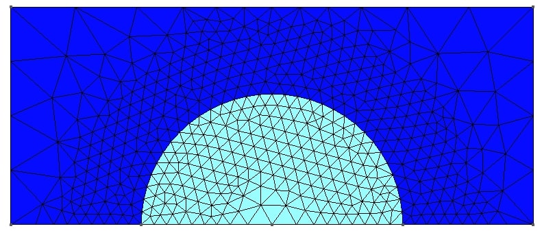
(a)

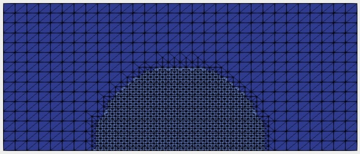
(b)

Figure 6: GMSH (a) and FEniCSx (b) generated meshes.

B.3 Import an external mesh (XDMF or MSH)

Once the mesh is generated as a tagged .msh or .xdmf file, one can consider directly read them to compile the domain and read the markers using:

⬇

from dolfinx.io.gmshio import read_from_msh

from dolfinx.io import XDMFFile

# set value to 0 if .xdmf, set it to 1 if .msh

mesher = 1

#

if mesher == 0:

##########################

## Read XDMF mesh ##

##########################

filename = "filename.xdmf"

with XDMFFile(MPI.COMM_WORLD, filename, "r") as file:

mesh = file.read_mesh()

mesh.topology.create_connectivity(mesh.topology.dim-1, mesh.topology.dim)

facet_tag = file.read_meshtags(mesh, "tag.name")

#

elif mesher == 1:

##########################

## Read gmsh mesh ##

##########################

mesh, cell_tag, facet_tag = read_from_msh("filename.msh", MPI.COMM_WORLD, 0, gdim=3)

#

else:

print(’The mesh type is wrongly defined. mesher should equal 0 for xdmf and 1 for msh files.’)

exit()

Appendix C Evaluate the function at a physical point

One strength of using FEniCSx is its ability to evaluate the solution at given points, summing the contribution of the neighbor cells of the mesh . The following code allowed to compute the figures presented for the results of the sections 3 and ref 4. First, one need to define the points where to evaluate the solution.

⬇

import numpy as np

num_points = 11

y_check = np.linspace(0,Height,num_points)

points_for_time = np.array([[Width/2, 0., 0.], [Width/2, Height/2, 0.]])

points_for_space = np.zeros((num_points,3))

for ii in range(num_points):

points_for_space[ii,0]=Width/2

points_for_space[ii,1]=y_check[ii]

points = np.concatenate((points_for_time,points_for_space))

The following step is to identify the cells contributing to the points.

⬇

from dolfinx.geometry import BoundingBoxTree, compute_collisions, compute_colliding_cells

tree = BoundingBoxTree(mesh, mesh.geometry.dim)

cell_candidates = compute_collisions(tree, points)

colliding_cells = compute_colliding_cells(mesh, cell_candidates, points)

# Here is an example to select cells contributing to the first and second points.

cells_y_0 = colliding_cells.links(0)

cells_y_H_over_2 = colliding_cells.links(1)

Knowing the shape of the functions to evaluate, lists are created and will be updated during the resolution procedure. Regarding parallel computation, these lists are only created on the first kernel.

⬇

from mpi4py import MPI

if MPI.COMM_WORLD.rank == 0:

pressure_y_0 = np.zeros(num_steps, dtype=PETSc.ScalarType)

pressure_y_Height_over_2 = np.zeros(num_steps, dtype=PETSc.ScalarType)

pressure_space0 = np.zeros(num_points, dtype=PETSc.ScalarType)

pressure_space1 = np.zeros(num_points, dtype=PETSc.ScalarType)

pressure_space2 = np.zeros(num_points, dtype=PETSc.ScalarType)

A function is created to evaluate a function given the mesh, the function, the contributing cells to the point and the list with its index to store the evaluated value in.

⬇

def evaluate_point(mesh, function, contributing_cells, point, output_list, index):

from mpi4py import MPI

function_eval = None

if len(contributing_cells) > 0:

function_eval = function.eval(point, contributing_cells[:1])

function_eval = mesh.comm.gather(function_eval, root=0)

# Choose first pressure that is found from the different processors

if MPI.COMM_WORLD.rank == 0:

for element in function_eval:

if element is not None:

output_list[index]=element[0]

break

pass

Finally, the problem is solved for each time steps. The functions are evaluated for all kernels and gathered on the first one where the first pressure found by the different processors will be uploaded in the here-above lists.

⬇

# time steps to evaluate the pressure in space:

n0, n1, n2 = 200,400,800

#

t = 0

L2_p = np.zeros(num_steps, dtype=PETSc.ScalarType)

for n in range(num_steps):

t += dt

try:

num_its, converged = solver.solve(X0)

except:

if MPI.COMM_WORLD.rank == 0:

print("*************")

print("Solver failed")

print("*************")

pass

X0.x.scatter_forward()

# Update Value

Xn.x.array[:] = X0.x.array

Xn.x.scatter_forward()

__u, __p = X0.split()

#

# Export the results

__u.name = "Displacement"

__p.name = "Pressure"

xdmf.write_function(__u,t)

xdmf.write_function(__p,t)

#

# Compute L2 norm for pressure

error_L2p = L2_error_p(mesh,pressure_element,__p)

L2_p[n] = error_L2p

#

# Solve tracking

if MPI.COMM_WORLD.rank == 0:

print(f"Time step {n}/{num_steps}, Load {T.value}, L2-error p {error_L2p:.2e}")

# Evaluate the functions

# in time

if n == n0:

for ii in range(num_points):

evaluate_point(mesh, __p, colliding_cells.links(ii+2), points[ii+2], pressure_space0, ii)

t0 = t

elif n==n1:

evaluate_point(mesh, __p, colliding_cells.links(ii+2), points[ii+2], pressure_space1, ii)

t1 = t

elif n==n2:

evaluate_point(mesh, __p, colliding_cells.links(ii+2), points[ii+2], pressure_space2, ii)

t2 = t

#

xdmf.close()

References

- Budday et al. [2019] S. Budday, T. C. Ovaert, G. A. Holzapfel, P. Steinmann, E. Kuhl, Fifty shades of brain: A review on the mechanical testing and modeling of brain tissue, Archives of Computational Methods in Engineering 27 (2019) 1187–1230. URL: https://doi.org/10.1007%2Fs11831-019-09352-w. doi:10.1007/s11831-019-09352-w.
- Hosseini-Farid et al. [2020] M. Hosseini-Farid, M. Ramzanpour, J. McLean, M. Ziejewski, G. Karami, A poro-hyper-viscoelastic rate-dependent constitutive modeling for the analysis of brain tissues, Journal of the Mechanical Behavior of Biomedical Materials 102 (2020) 103475. URL: {}{}}{https://doi.org/10.1016/j.jmbbm.2019.103475}{cmtt}. doi:10.1016/j.jmbbm.2019.103475.
- Franceschini et~al. [2006] G.~Franceschini, D.~Bigoni, P.~Regitnig, G.~Holzapfel, Brain tissue deforms similarly to filled elastomers and follows consolidation theory, Journal of the Mechanics and Physics of Solids 54 (2006) 2592--2620. URL: {}{}}{https://doi.org/10.1016/j.jmps.2006.05.004}{cmtt}. doi:10.1016/j.jmps.2006.05.004.
- Urcun et~al. [2022] S.~Urcun, P.-Y. Rohan, G.~Sciumè, S.~P. Bordas, Cortex tissue relaxation and slow to medium load rates dependency can be captured by a two-phase flow poroelastic model, Journal of the Mechanical Behavior of Biomedical Materials 126 (2022) 104952. URL: https://www.sciencedirect.com/science/article/pii/S175161612100583X. doi:https://doi.org/10.1016/j.jmbbm.2021.104952.
- Lavigne et~al. [2022] T.~Lavigne, G.~Sciumè, S.~Laporte, H.~Pillet, S.~Urcun, B.~Wheatley, P.-Y. Rohan, Société de biomécanique young investigator award 2021: Numerical investigation of the time-dependent stress–strain mechanical behaviour of skeletal muscle tissue in the context of pressure ulcer prevention, Clinical Biomechanics 93 (2022) 105592. URL: https://www.sciencedirect.com/science/article/pii/S0268003322000225. doi:https://doi.org/10.1016/j.clinbiomech.2022.105592.
- Sciumè et~al. [2013] G.~Sciumè, S.~Shelton, W.~G. Gray, C.~T. Miller, F.~Hussain, M.~Ferrari, P.~Decuzzi, B.~A. Schrefler, A multiphase model for three-dimensional tumor growth, New Journal of Physics 15 (2013) 015005. URL: {}{}}{https://doi.org/10.1088/1367-2630/15/1/015005}{cmtt}. doi:10.1088/1367-2630/15/1/015005.
- Sciumè [2021] G.~Sciumè, Mechanistic modeling of vascular tumor growth: an extension of biot's theory to hierarchical bi-compartment porous medium systems, Acta Mechanica 232 (2021) 1445--1478. URL: {https://doi.org/10.1007/s00707-020-02908-z}. doi:10.1007/s00707-020-02908-z.
- Oftadeh et~al. [2018] R.~Oftadeh, B.~K. Connizzo, H.~T. Nia, C.~Ortiz, A.~J. Grodzinsky, Biological connective tissues exhibit viscoelastic and poroelastic behavior at different frequency regimes: Application to tendon and skin biophysics, Acta Biomaterialia 70 (2018) 249--259. URL: https://www.sciencedirect.com/science/article/pii/S1742706118300527. doi:https://doi.org/10.1016/j.actbio.2018.01.041.
- Ateshian [2009] G.~A. Ateshian, The role of interstitial fluid pressurization in articular cartilage lubrication, Journal of Biomechanics 42 (2009) 1163--1176. URL: https://www.sciencedirect.com/science/article/pii/S0021929009002565. doi:https://doi.org/10.1016/j.jbiomech.2009.04.040.
- Argoubi and Shirazi-Adl [1996] M.~Argoubi, A.~Shirazi-Adl, Poroelastic creep response analysis of a lumbar motion segment in compression, Journal of Biomechanics 29 (1996) 1331--1339. URL: {}{}}{https://doi.org/10.1016/0021-9290(96)00035-8}{cmtt}. doi:10.1016/0021-9290(96)00035-8.
- Gimnich et~al. [2019] O.~A. Gimnich, J.~Singh, J.~Bismuth, D.~J. Shah, G.~Brunner, Magnetic resonance imaging based modeling of microvascular perfusion in patients with peripheral artery disease, Journal of Biomechanics 93 (2019) 147--158. URL: {}{}}{https://doi.org/10.1016/j.jbiomech.2019.06.025}{cmtt}. doi:10.1016/j.jbiomech.2019.06.025.
- Peyrounette et~al. [2018] M.~Peyrounette, Y.~Davit, M.~Quintard, S.~Lorthois, Multiscale modelling of blood flow in cerebral microcirculation: Details at capillary scale control accuracy at the level of the cortex, PLOS ONE 13 (2018) e0189474. URL: {}{}}{https://doi.org/10.1371/journal.pone.0189474}{cmtt}. doi:10.1371/journal.pone.0189474.
- Siddique et~al. [2017] J.~Siddique, A.~Ahmed, A.~Aziz, C.~Khalique, A review of mixture theory for deformable porous media and applications, Applied Sciences 7 (2017) 917. URL: {}{}}{https://doi.org/10.3390/app7090917}{cmtt}. doi:10.3390/app7090917.
- Van Loocke et~al. [2009] M.~Van Loocke, C.~Simms, C.~Lyons, Viscoelastic properties of passive skeletal muscle in compression—cyclic behaviour, Journal of Biomechanics 42 (2009) 1038--1048. URL: {}{}}{https://doi.org/10.1016/j.jbiomech.2009.02.022}{cmtt}. doi:10.1016/j.jbiomech.2009.02.022.
- Simms et~al. [2012] C.~K. Simms, M.~V. Loocke, C.~G. Lyons, SKELETAL MUSCLE IN COMPRESSION: MODELING APPROACHES FOR THE PASSIVE MUSCLE BULK, International Journal for Multiscale Computational Engineering 10 (2012) 143--154. URL: {}{}}{https://doi.org/10.1615/intjmultcompeng.2011002419}{cmtt}. doi:10.1615/intjmultcompeng.2011002419.
- Wheatley et~al. [2015] B.~B. Wheatley, R.~B. Pietsch, T.~L.~H. Donahue, L.~N. Williams, Fully non-linear hyper-viscoelastic modeling of skeletal muscle in compression, Computer Methods in Biomechanics and Biomedical Engineering 19 (2015) 1181--1189. URL: {}{}}{https://doi.org/10.1080/10255842.2015.1118468}{cmtt}. doi:10.1080/10255842.2015.1118468.
- Vaidya and Wheatley [2020] A.~J. Vaidya, B.~B. Wheatley, An experimental and computational investigation of the effects of volumetric boundary conditions on the compressive mechanics of passive skeletal muscle, Journal of the Mechanical Behavior of Biomedical Materials 102 (2020) 103526. URL: {}{}}{https://doi.org/10.1016/j.jmbbm.2019.103526}{cmtt}. doi:10.1016/j.jmbbm.2019.103526.
- Urcun et~al. [2021] S.~Urcun, P.-Y. Rohan, W.~Skalli, P.~Nassoy, S.~P.~A. Bordas, G.~Sciumè, Digital twinning of cellular capsule technology: Emerging outcomes from the perspective of porous media mechanics, PLOS ONE 16 (2021) 1--30. URL: {}{}}{https://doi.org/10.1371/journal.pone.0254512}{cmtt}. doi:10.1371/journal.pone.0254512.
- Gray and Miller [2014] W.~G. Gray, C.~T. Miller, Introduction to the Thermodynamically Constrained Averaging Theory for Porous Medium Systems, Springer International Publishing, 2014. URL: {}{}}{https://doi.org/10.1007/978-3-319-04010-3}{cmtt}. doi:10.1007/978-3-319-04010-3.
- Mascheroni et~al. [2016] P.~Mascheroni, C.~Stigliano, M.~Carfagna, D.~P. Boso, L.~Preziosi, P.~Decuzzi, B.~A. Schrefler, Predicting the growth of glioblastoma multiforme spheroids using a multiphase porous media model, Biomechanics and Modeling in Mechanobiology 15 (2016) 1215--1228. URL: {}{}}{https://doi.org/10.1007/s10237-015-0755-0}{cmtt}. doi:10.1007/s10237-015-0755-0.
- Fehervary et~al. [2020] H.~Fehervary, L.~Maes, J.~Vastmans, G.~Kloosterman, N.~Famaey, How to implement user-defined fiber-reinforced hyperelastic materials in finite element software, Journal of the Mechanical Behavior of Biomedical Materials 110 (2020) 103737. URL: https://www.sciencedirect.com/science/article/pii/S1751616120302915. doi:https://doi.org/10.1016/j.jmbbm.2020.103737.
- Zulian et~al. [2021] P.~Zulian, A.~Kopaničáková, M.~G.~C. Nestola, N.~Fadel, A.~Fink, J.~VandeVondele, R.~Krause, Large scale simulation of pressure induced phase‐field fracture propagation using Utopia, CCF Transactions on High Performance Computing (2021). URL: https://doi.org/10.1007/s42514-021-00069-6. doi:10.1007/s42514-021-00069-6. arXiv:https://doi.org/10.1007/s42514-021-00069-6.
- Zulian et~al. [2016] P.~Zulian, A.~Kopaničáková, M.~C.~G. Nestola, A.~Fink, N.~Fadel, A.~Rigazzi, V.~Magri, T.~Schneider, E.~Botter, J.~Mankau, R.~Krause, Utopia: A performance portable C++ library for parallel linear and nonlinear algebra. Git repository, https://bitbucket.org/zulianp/utopia, 2016. URL: https://bitbucket.org/zulianp/utopia.
- Alnæs et~al. [2015] M.~Alnæs, J.~Blechta, J.~Hake, A.~Johansson, B.~Kehlet, A.~Logg, C.~Richardson, J.~Ring, M.~E. Rognes, G.~N. Wells, The fenics project version 1.5, <p>Archive of Numerical Software Vol 3 (2015) <strong>Starting Point and Frequency: </strong>Year: 2013</p>. URL: http://journals.ub.uni-heidelberg.de/index.php/ans/article/view/20553. doi:10.11588/ANS.2015.100.20553.
- Mazier et~al. [2022] A.~Mazier, S.~E. Hadramy, J.-N. Brunet, J.~S. Hale, S.~Cotin, S.~P.~A. Bordas, Sonics: Develop intuition on biomechanical systems through interactive error controlled simulations, 2022. URL: https://arxiv.org/abs/2208.11676. doi:10.48550/ARXIV.2208.11676.
- Mazier et~al. [2021] A.~Mazier, S.~Ribes, B.~Gilles, S.~P. Bordas, A rigged model of the breast for preoperative surgical planning, Journal of Biomechanics 128 (2021) 110645. URL: https://www.sciencedirect.com/science/article/pii/S0021929021004140. doi:https://doi.org/10.1016/j.jbiomech.2021.110645.
- Bulle [2022] R.~Bulle, A posteriori error estimation for finite element approximations of fractional Laplacian problems and applications to poro-elasticity, Theses, University of Luxembourg ; Université de Bourgogne Franche-Comté, 2022. URL: https://tel.archives-ouvertes.fr/tel-03652547.
- Haagenson et~al. [2020] R.~Haagenson, H.~Rajaram, J.~Allen, A generalized poroelastic model using FEniCS with insights into the noordbergum effect, Computer Methods in Applied Mechanics and Engineering 135 (2020) 104399. URL: https://doi.org/10.1016/j.cageo.2019.104399. doi:10.1016/j.cageo.2019.104399.
- Joodat et~al. [2018] S.~Joodat, K.~Nakshatrala, R.~Ballarini, Modeling flow in porous media with double porosity/permeability: A stabilized mixed formulation, error analysis, and numerical solutions, Computer Methods in Applied Mechanics and Engineering 337 (2018) 632--676. URL: https://www.sciencedirect.com/science/article/pii/S0045782518301749. doi:https://doi.org/10.1016/j.cma.2018.04.004.
- Alnæs et~al. [2014] M.~S. Alnæs, A.~Logg, K.~B. Ølgaard, M.~E. Rognes, G.~N. Wells, Unified form language: A domain-specific language for weak formulations of partial differential equations, ACM Trans. Math. Softw. 40 (2014). URL: https://doi.org/10.1145/2566630. doi:10.1145/2566630.
- Scroggs et~al. [2022a] M.~W. Scroggs, J.~S. Dokken, C.~N. Richardson, G.~N. Wells, Construction of arbitrary order finite element degree-of-freedom maps on polygonal and polyhedral cell meshes, ACM Trans. Math. Softw. 48 (2022a). URL: https://doi.org/10.1145/3524456. doi:10.1145/3524456.
- Scroggs et~al. [2022b] M.~W. Scroggs, I.~A. Baratta, C.~N. Richardson, G.~N. Wells, Basix: a runtime finite element basis evaluation library, Journal of Open Source Software 7 (2022b) 3982. URL: https://doi.org/10.21105/joss.03982. doi:10.21105/joss.03982.
- Geuzaine and Remacle [2018] C.~Geuzaine, J.-F. Remacle, Gmsh, 2018. URL: http://http://gmsh.info/.
- Selvadurai and Suvorov [2016] A.~Selvadurai, A.~Suvorov, Coupled hydro-mechanical effects in a poro-hyperelastic material, Journal of the Mechanics and Physics of Solids 91 (2016) 311--333. URL: https://www.sciencedirect.com/science/article/pii/S0022509615303574. doi:https://doi.org/10.1016/j.jmps.2016.03.005.
- Treloar [1975] L.~G. Treloar, The physics of rubber elasticity, OUP Oxford, 1975.
- Simo [1988] J.~Simo, A framework for finite strain elastoplasticity based on maximum plastic dissipation and the multiplicative decomposition: Part i. continuum formulation, Computer Methods in Applied Mechanics and Engineering 66 (1988) 199--219. URL: https://www.sciencedirect.com/science/article/pii/004578258890076X. doi:https://doi.org/10.1016/0045-7825(88)90076-X.
- Horgan and Saccomandi [2004] C.~O. Horgan, G.~Saccomandi, Constitutive models for compressible nonlinearly elastic materials with limiting chain extensibility, Journal of Elasticity 77 (2004) 123--138. URL: https://doi.org/10.1007/s10659-005-4408-x. doi:10.1007/s10659-005-4408-x.
- Marino [2018] M.~Marino, Constitutive Modeling of Soft Tissues, 2018, p. 81–110. doi:10.1016/B978-0-12-801238-3.99926-4.
- Pence and Gou [2014] T.~J. Pence, K.~Gou, On compressible versions of the incompressible neo-hookean material, Mathematics and Mechanics of Solids 20 (2014) 157--182. URL: https://doi.org/10.1177/1081286514544258. doi:10.1177/1081286514544258.
- Doll and Schweizerhof [2000] S.~Doll, K.~Schweizerhof, On the development of volumetric strain energy functions, J. Appl. Mech. 67 (2000) 17--21.