The multifaceted nature of uncertainty in structure-property linkage with crystal plasticity finite element model

Abstract

Uncertainty quantification (UQ) plays a critical role in verifying and validating forward integrated computational materials engineering (ICME) models. Among numerous ICME models, the crystal plasticity finite element method (CPFEM) is a powerful tool that enables one to assess microstructure-sensitive behaviors and thus, bridge material structure to performance. Nevertheless, given its nature of constitutive model form and the randomness of microstructures, CPFEM is exposed to both aleatory uncertainty (microstructural variability), as well as epistemic uncertainty (parametric and model-form error). Therefore, the observations are often corrupted by the microstructure-induced uncertainty, as well as the ICME approximation and numerical errors. In this work, we highlight several ongoing research topics in UQ, optimization, and machine learning applications for CPFEM to efficiently solve forward and inverse problems.

The first aspect of this work addresses the UQ of constitutive models for epistemic uncertainty, including both phenomenological and dislocation-density-based constitutive models, where the quantities of interest (QoIs) are related to the initial yield behaviors. We apply a stochastic collocation (SC) method to quantify the uncertainty of the three most commonly used constitutive models in CPFEM, namely phenomenological models (with and without twinning), and dislocation-density-based constitutive models, for three different types of crystal structures, namely face-centered cubic (fcc) copper (Cu), body-centered cubic (bcc) tungsten (W), and hexagonal close packing (hcp) magnesium (Mg).

The second aspect of this work addresses the aleatory and epistemic uncertainty with multiple mesh resolutions and multiple constitutive models by the multi-index Monte Carlo method, where the QoI is also related to homogenized materials properties. We present a unified approach that accounts for various fidelity parameters, such as mesh resolutions, integration time-steps, and constitutive models simultaneously. We illustrate how multilevel sampling methods, such as multilevel Monte Carlo (MLMC) and multi-index Monte Carlo (MIMC), can be applied to assess the impact of variations in the microstructure of polycrystalline materials on the predictions of macroscopic mechanical properties.

The third aspect of this work addresses the crystallographic texture study of a single void in a cube. Using a parametric reduced-order model (also known as parametric proper orthogonal decomposition) with a global orthonormal basis as a model reduction technique, we demonstrate that the localized dynamic stress and strain fields can be predicted as a spatiotemporal problem.

The fourth aspect of this work highlights the constitutive model calibration using an optimization under microstructure-induced uncertainty with Bayesian optimization. To account for natural variability or the aleatory uncertainty of microstructure, we average the loss function over an ensemble of microstructures and couple the Monte Carlo estimator with an asynchronous parallel Bayesian optimization to calibrate a phenomenological constitutive model. The framework is demonstrated for 304L stainless steel.

The fifth aspect of this work solves a stochastic inverse problem in the structure-property relationship. In this aspect, we seek to consistently learn a distribution of microstructure features, in the sense that the forward propagation of this microstructure feature distribution through CPFEM matches a target distribution of homogenized materials properties.

1 Introduction

Process-structure-property relationship is the hallmark of materials science across multiple length-scales and time-scales. Along with experimental materials science, numerous integrated computational materials engineering (ICME) models have been developed over the last several decades to accurately predict and reliably quantify uncertainty for the prediction. The computational ICME approach and the emerging physics-informed and physics-constrained machine learning (ML) in materials science have significantly accelerated the materials design process to tailor materials properties depending on the need [1]. For materials science, uncertainty quantification (UQ) is an essential part, since microstructures are inherently noisy and can only be captured by statistical microstructure descriptors. Optimization (Opt) also plays an important role, mainly in calibrating ICME models to establish a predictive science process. The computer predictions with quantified uncertainty have long been visioned [2, 3], and it still holds true for ICME in computational materials science.

For structure-property relationship, phase-field and crystal plasticity finite element model (CPFEM) are arguably the most successful computational tools to numerically investigate different materials phenomena. In this paper, we highlight several on-going research efforts in UQ, optimization, and ML applications for CPFEM. The numerical implementations are mainly done through DREAM.3D [4] and DAMASK [5, 6]. The first code coupling was demonstrated in [7].

The remaining of the paper is organized as follows. Section 2 quantifies uncertainty with respect to three different constitutive models for initial yield behaviors. Section 3 applied multi-level/multi-index Monte Carlo (MLMC/MIMC) approach to quantify uncertainty for homogenized materials properties. Section 4 develops a parametric reduced-order model using proper-orthogonal decomposition method to emulate the full-field stress-strain response of a void model. Section 5 demonstrates the asynchronous parallel Bayesian optimization to calibrate a phenomenological constitutive model for stainless steel 304L. Section 6 applies a data-consistent stochastic inverse UQ technique to infer a distribution of microstructure features such that the forward propagation through CPFEM matches a target distribution of homogenized materials properties. Section 7 discusses and concludes the paper.

2 UQ of constitutive models in CPFEM

In this section, we highlight our recent effort [8] in quantifying epistemic uncertainty associated with initial yield behaviors, which are characterized by yield strength $\displaystyle\varepsilon_{\text{Y}}$ and yield stress $\displaystyle\sigma_{\text{Y}}$ at 0.2% offset. In this approach, we impose a uniform prior for all constitutive model parameters. Three constitutive models are considered in this study: phenomenological constitutive model with and without twinning, dislocation-density-based constitutive model. Interested readers are referred to the DAMASK paper [6] (cf. Section 6) for more modeling description regarding for constitutive models.

The generalized Wiener-Askey polynomial chaos expansion [9] represents the second-order random process $\displaystyle f(\theta)$ as

$$\begin{array}[]{lll}f(\theta)&=&c_{0}I_{0}+\sum_{i_{1}=1}^{\infty}c_{i_{1}}I_{1}(\xi_{i_{1}}(\theta))\\ &+&\sum_{i_{1}=1}^{\infty}\sum_{i_{2}=1}^{\infty}c_{i_{1}i_{2}}I_{2}(\xi_{i_{1}}(\theta),\xi_{i_{2}}(\theta))\\ &+&\sum_{i_{1}=1}^{\infty}\sum_{i_{2}=1}^{\infty}\sum_{i_{3}=1}^{\infty}c_{i_{1}i_{2}i_{3}}I_{3}(\xi_{i_{1}}(\theta),\xi_{i_{2}}(\theta),\xi_{i_{3}}(\theta))+\cdots,\end{array}$$ (1)

where $\displaystyle I_{n}(\xi_{i_{1}},\cdots,\xi_{i_{n}})$ denotes the Wiener-Askey polynomial chaos of order $\displaystyle n$ in terms of the random vector $\displaystyle\boldsymbol{\xi}=(\xi_{i_{1}},\xi_{i_{2}},\dots,\xi_{i_{n}})$, and $\displaystyle c$’s are polynomial chaos expansion coefficients to be determined. Without loss of generality, Equation 1 can be rewritten as

$$f(\theta)=\sum_{j=0}^{\infty}\widehat{f}_{j}\boldsymbol{\Phi}_{j}(\boldsymbol{\xi(\theta)}),$$ (2)

where there is a one-to-one correspondence between the function $\displaystyle I_{n}(\xi_{i_{1}},\cdots,\xi_{i_{n}})$ and $\displaystyle\boldsymbol{\Phi}_{j}(\boldsymbol{\xi})$.

Table 1 describes the relationship between the types of Wiener-Askey polynomial chaos and their corresponding underlying random variables. For uniformly distributed variables $\displaystyle\boldsymbol{\xi}$ used in this paper, the Wiener-Askey scheme [9] requires Legendre polynomials as the polynomial basis $\displaystyle\{\boldsymbol{\Phi}_{j}\}$.

Table 1: Relationship between the types of Wiener-Askey polynomial chaos and their underlying random variables $\displaystyle\theta$

random variable	probability density function	polynomial	support range
Gaussian	$\displaystyle\frac{1}{\sqrt{2\pi}}e^{-\frac{\theta^{2}}{2}}$	Hermite	$\displaystyle(-\infty,\infty)$
uniform	$\displaystyle\frac{1}{2}$	Legendre	$\displaystyle[-1,1]$
beta	$\displaystyle\frac{(1-\theta)^{\alpha}(1+\theta)^{\beta}}{2^{\alpha+\beta+1}B(\alpha+1,\beta+1)}$	Jacobi	$\displaystyle[-1,1]$
gamma	$\displaystyle\frac{\theta^{\alpha}e^{-\theta}}{\Gamma(\alpha+1)}$	Laguerre	$\displaystyle[0,\infty)$

To mitigate the curse of dimensionality, we employ stochastic collocation method [10, 11, 12] to evaluate numerical integration on Gaussian abscissas and compute the polynomial chaos expansion coefficients using Smolyak sparse grid [13, 14, 15, 16].

Following [17], [18], and [19], we summarize the variance-based global sensitivity analysis based on Sobol’ decomposition as follows. In the spirit of generalized polynomial chaos expansion (i.e. Equation 1 after finite truncation), the Sobol’ decomposition of $\displaystyle f(\boldsymbol{\xi})$ into the summands of increasing dimensions as

$$\begin{array}[]{lll}f(\xi_{1},\dots,\xi_{n})&=&f_{0}+\sum_{i=1}^{n}\sum_{\alpha\in\mathscr{I}_{1}}f_{\alpha}{\boldsymbol{\Phi}}(\xi_{i})\\ &&+\sum_{1\leq i_{1}<i_{2}\leq n}\sum_{\alpha\in\mathscr{I}_{i_{1}i_{2}}}f_{\alpha}\boldsymbol{\Phi}(\xi_{i_{1}},\xi_{i_{2}})+\cdots\\ &&+\sum_{1\leq i_{1}<\cdots<i_{s}\leq n}\sum_{\alpha\in\mathscr{I}_{i_{1},\dots,i_{s}}}f_{\alpha}\boldsymbol{\Phi}(\xi_{i_{1}},\dots,\xi_{i_{s}})\\ &&+\cdots+\sum_{\alpha\in\mathscr{I}_{1,2,\dots,n}}f_{\alpha}\boldsymbol{\Phi}(\xi_{1},\dots,\xi_{n}).\end{array}$$ (3)

Given a model of the form $\displaystyle y=f(\xi_{1},\xi_{2},\dots,\xi_{n})$, with $\displaystyle y$ as a scalar, a variance-based first order effect for a generic factor $\displaystyle\xi_{i}$ can be written as $\displaystyle\mathbb{V}_{\xi_{i}}\left[\mathbb{E}_{\boldsymbol{\xi}_{\sim i}}\left[y|\xi_{i}\right]\right]$, where $\displaystyle\boldsymbol{\xi}_{\sim i}$ is the vector $\displaystyle\boldsymbol{\xi}$ without the $\displaystyle i$-th element, i.e. $\displaystyle\boldsymbol{\xi}_{\sim i}=(\xi_{1},\dots,\xi_{i-1},\xi_{i+1},\dots,\xi_{n})$. The main effect sensitivity index (first-order sensitivity coefficient) is written as

$$S_{i}=\frac{\mathbb{V}_{\xi_{i}}\left[\mathbb{E}_{\boldsymbol{\xi}_{\sim i}}\left[y|\xi_{i}\right]\right]}{\mathbb{V}[y]}.$$ (4)

It is relatively well-known that

$$\mathbb{E}\left[\mathbb{V}\left[y|\boldsymbol{\xi}_{\sim i}\right]\right]+\mathbb{V}\left[\mathbb{E}\left[y|\boldsymbol{\xi}_{\sim i}\right]\right]=\mathbb{V}[y],$$ (5)

and therefore, the total effect sensitivity index can be obtained as

$$T_{i}=\frac{\mathbb{E}\left[\mathbb{V}\left[y|\boldsymbol{\xi}_{\sim i}\right]\right]}{\mathbb{V}[y]}=1-\frac{\mathbb{V}\left[\mathbb{E}\left[y|\boldsymbol{\xi}_{\sim i}\right]\right]}{\mathbb{V}[y]}.$$ (6)

For interested readers, more details and implementation are available in Tang et al. [20] and Crestaux et al. [18], where most of the computations are based on Monte Carlo sampling $\displaystyle\boldsymbol{\xi}$. In the context of this section, we can understand $\displaystyle\boldsymbol{\xi}$ as the set of parameters for the underlying constitutive model, whether it is phenomenological or dislocation-density-based, and $\displaystyle y$ as the quantity of interest from the CPFEM model.

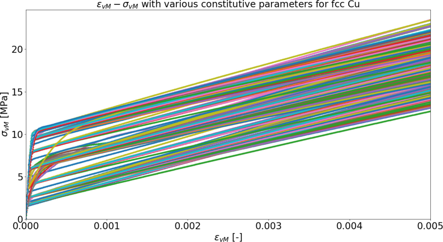
(a) fcc Cu.

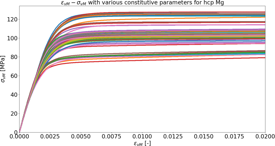
(b) hcp Mg.

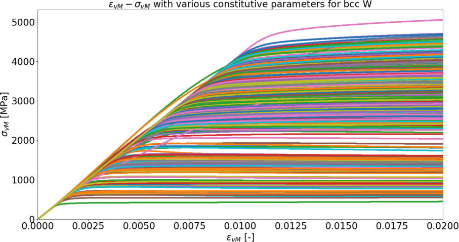
(c) bcc W.

Figure 1: Equivalent von Mises stress-strain plots. Reprinted from [8].

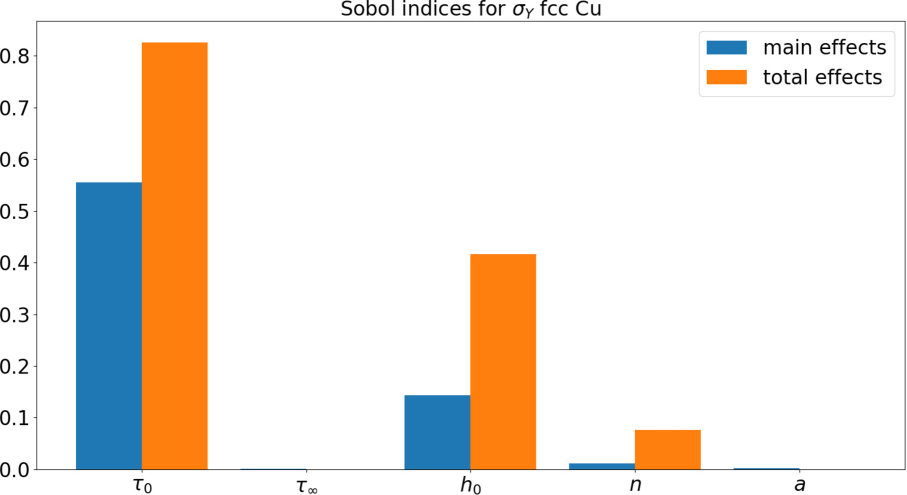
(a) Sobol’ indices for $\displaystyle\sigma_{\text{Y}}$ for fcc Cu.

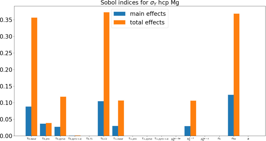
(b) Sobol’ indices for $\displaystyle\varepsilon_{\text{Y}}$ for hcp Mg.

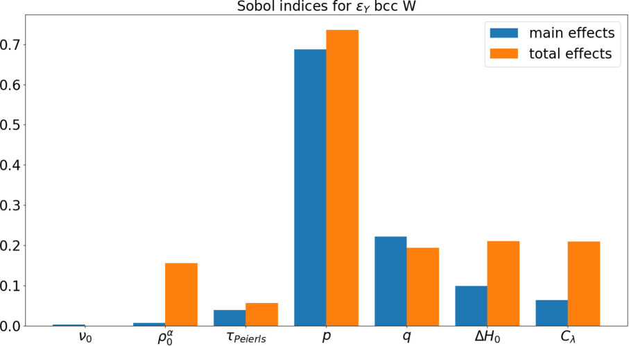
(c) Sobol’ indices for $\displaystyle\varepsilon_{\text{Y}}$ for bcc W.

Figure 2: Global sensitivity analysis with Sobol’ indices for different constitutive models. Reprinted from [8].

3 Multi-fidelity microstructure-induced UQ for CPFEM

The second aspect highlights our recent research effort in exploiting the well-posed fidelity hierarchy in CPFEM that is often overlooked in the literature to quantify aleatory and epistemic uncertainty. The aleatory uncertainty originates from the SERVE instantiation, whereas the epistemic uncertainty originates from the mesh discretization for SERVEs and the plasticity constitutive model. In this research thrust, we apply a relatively well-known Monte Carlo, called multi-level Monte Carlo [21, 22] and its multi-dimensional extension called multi-index Monte Carlo [23, 24, 25], to estimate a homogenized materials property in an efficient manner.

(a) $\displaystyle 8^{3}$: DDB.

(b) $\displaystyle 16^{3}$: DDB.

(c) $\displaystyle 20^{3}$: DDB.

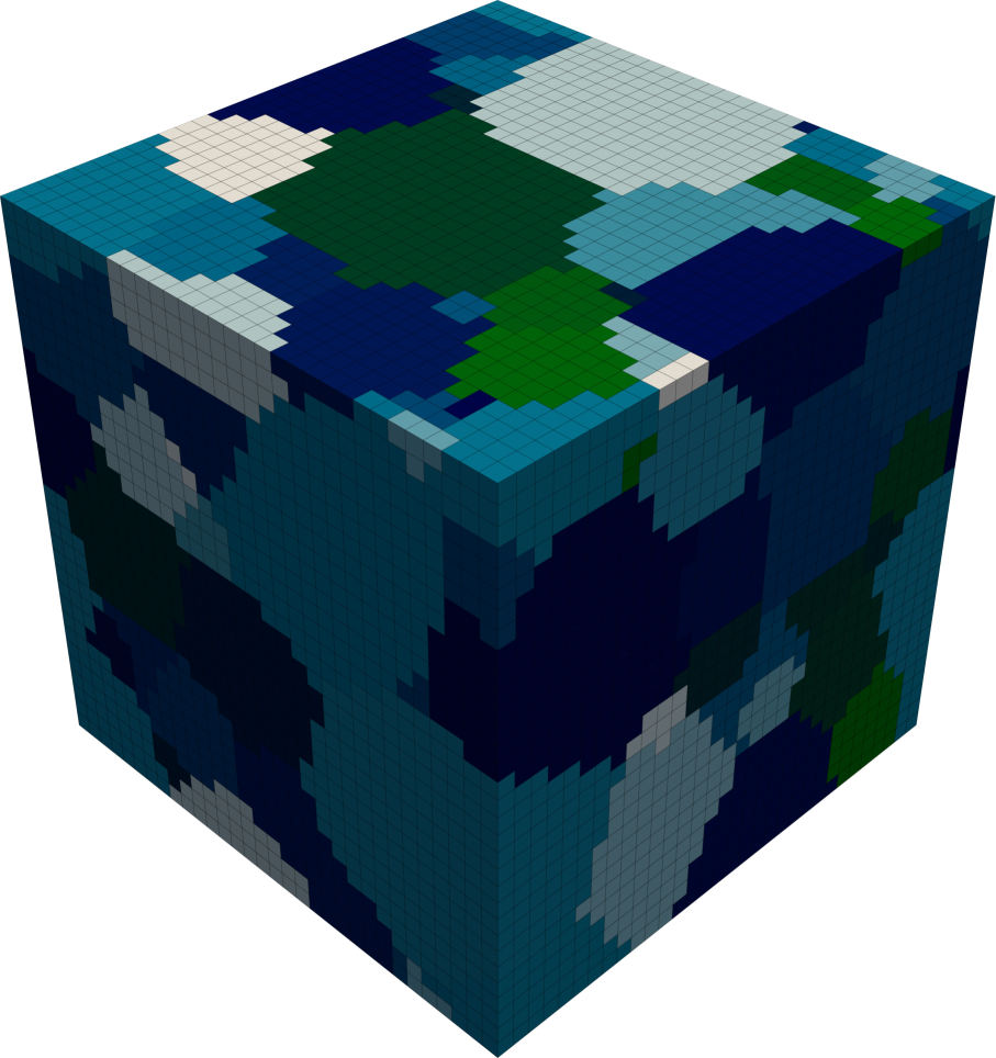
(d) $\displaystyle 32^{3}$: DDB.

(e) $\displaystyle 64^{3}$: DDB.

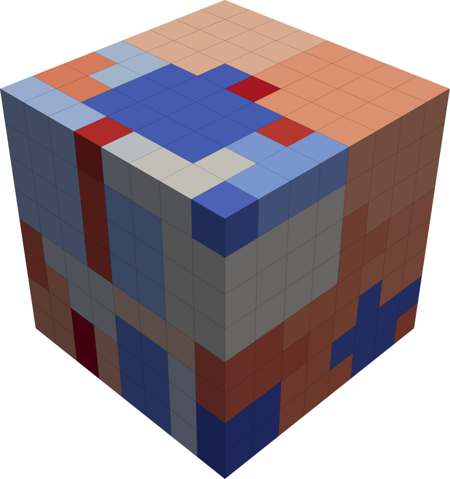
(f) $\displaystyle 8^{3}$: Phen.

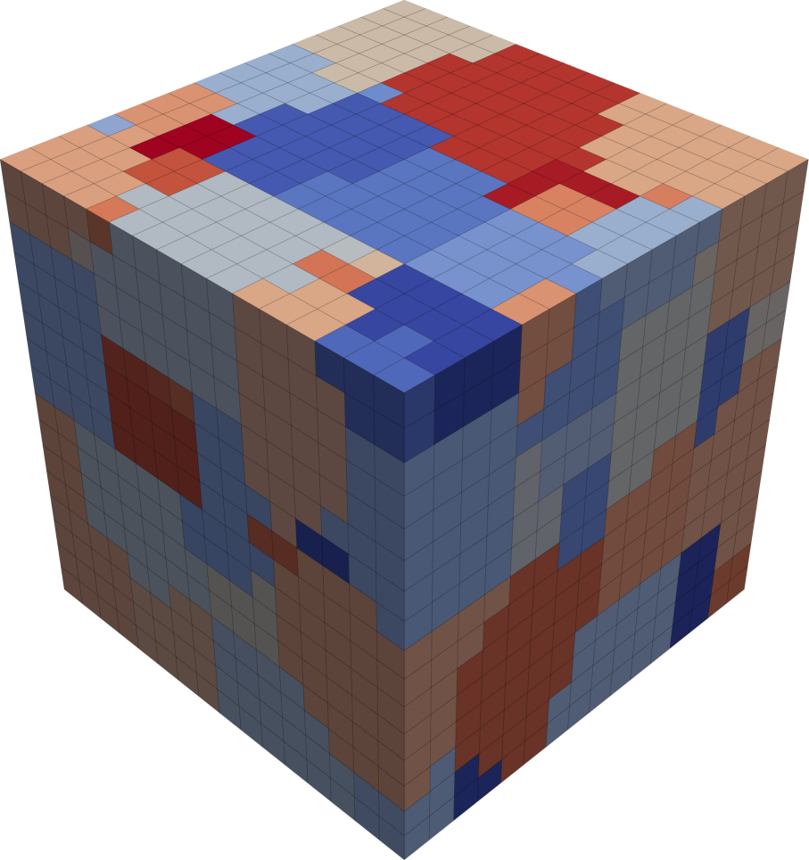
(g) $\displaystyle 16^{3}$: Phen.

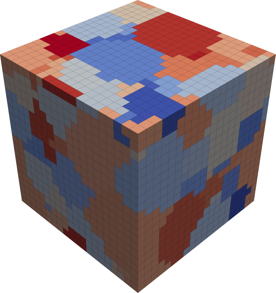
(h) $\displaystyle 20^{3}$: Phen.

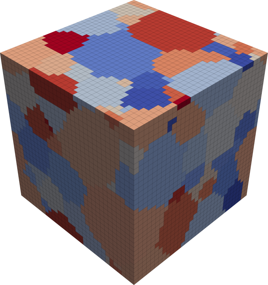
(i) $\displaystyle 32^{3}$: Phen.

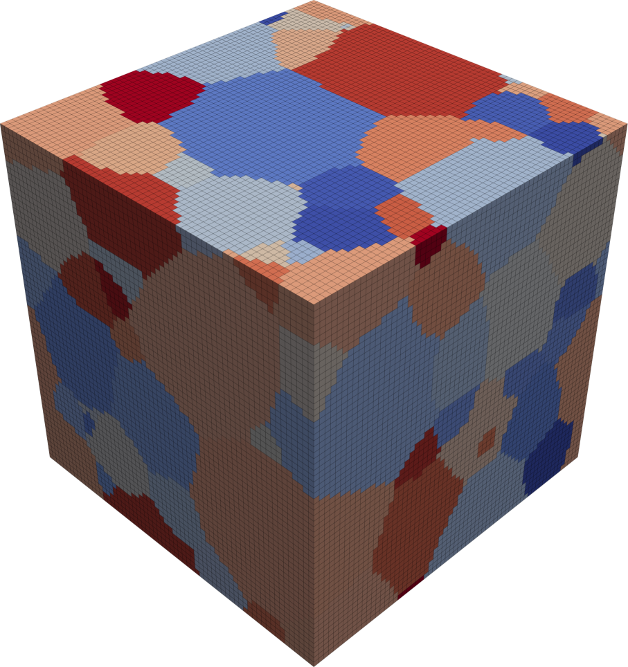
(j) $\displaystyle 64^{3}$: Phen.

Figure 3: A schematic illustration of multi-index Monte Carlo in CPFEM with 2-dimensional fidelity level. The first fidelity variable corresponds to the mesh resolution, whereas the second fidelity variable corresponds to the constitutive plasticity model. The first fidelity variable (i.e. mesh resolution) increases from the left to the right, where as the second fidelity variable (i.e. constitutive model) increases from the bottom to the top. The low-fidelity constitutive model is phenomenological constitutive model (Phen) and the high-fidelity constitutive model is dislocation-density-based (DDB) constitutive model.

In the MLMC case study, we consider an exemplar application of statistically equivalent representative volume elements (SERVEs), where the mesh discretization could be very coarse or very fine for $\displaystyle\alpha$-Titanium. In the MIMC case study, we consider the extended version of the MLMC case study, where the first fidelity variable corresponds to the mesh resolution and the second variable corresponds to the constitutive models for an aluminum alloy. The phenomenological constitutive model is considered as the low-fidelity model, whereas the dislocation-density-based constitutive model is considered as the high-fidelity model. Figure 3 shows a schematic illustration of MIMC in two directions: the first direction – from left to right – corresponds to the mesh resolution, the second direction – from bottom to top – corresponds to the constitutive model.

Figure 4: Cost of the adaptive MIMC and MLMC methods compared to the (estimated) complexity of the single-level MC method, expressed in terms of the total simulation time in seconds, as a function of the tolerance $\displaystyle\varepsilon$ on the root mean-square error. For the target root mean-square error tolerance of $\displaystyle\varepsilon=5$, the MLMC method is approximately $\displaystyle 11.6$ times faster than the MC method, and the adaptive MIMC method is $\displaystyle 2.7$ times faster than the MLMC method, resulting in a final speedup of adaptive MIMC over MC of $\displaystyle 31.5\times$.

Figure 4 compares the convergence behaviors of the Monte Carlo, MLMC, and adaptive MIMC estimators, respectively. For the MIMC case study, where the QoI is the effective Young modulus, with the root mean-square error $\displaystyle\varepsilon=5$GPa, we demonstrate that the adaptive MIMC estimator is $\displaystyle 2.7\times$ faster than the MLMC estimator, and the MLMC is $\displaystyle 11.6\times$ faster than the MC estimator. By using an adaptive mesh resolution and an adaptive constitutive model, the homogenized materials properties can be estimated more efficiently and accurately with an unbiased estimator.

4 A parametric ROM for void model

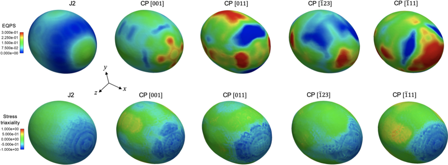
Figure 5: Stress triaxiality for different crystal orientations.

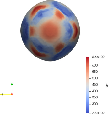
(a) Reduced-order model.

(b) Full-order model.

Figure 6: Comparison between reduced-order model (Figure 6(a)) and full-order model (Figure 6(b)) in the $\displaystyle[\overline{1}11]$ direction shows an excellent agreement between reduced-order model and full-order model.

In the third aspect, we develop a projection-based reduced-order model for single crystal void model using CPFEM, mainly following [26]. The idea behind is to decompose the random vector field $\displaystyle\mathbf{u}(\mathbf{x},t;\mathbf{p})$, in the spirit of Karhunen-Loève expansion, into a set of deterministic spatial functions $\displaystyle\mathbf{l}_{k}(\mathbf{x})$ modulated by parameterized random time coefficients $\displaystyle\mathbf{q}(t;\mathbf{p})$ so that

$$\mathbf{u}(\mathbf{x},t;\mathbf{p})=\sum_{k=1}^{\infty}\mathbf{q}(t;\mathbf{p})\mathbf{l}_{k}(\mathbf{x}).$$ (7)

Originally introduced by Sirovich [27], the method of snapshots consider a set of snapshots $\displaystyle\mathbf{u}_{1},\mathbf{u}_{2},\dots,\mathbf{u}_{m}\in\mathbb{R}^{n}$ of state solutions computed at different instants in time and different orientations $\displaystyle\mathbf{p}$ (parametrized either as Euler angles $\displaystyle(\rho_{1},\Phi,\rho_{2})$ or generalized spherical harmonics coefficients, which is a robust and effective way to represent textures and orientations in polycrystalline materials [28, 29]), where $\displaystyle\mathbf{u}_{j}\in\mathbb{R}^{n}$ denotes the $\displaystyle j$-th snapshot and one collects $\displaystyle m<n$ snapshots, where $\displaystyle n$ is typically large and in particular, (much) larger than the number of snapshots. Define the snapshot matrix $\displaystyle\mathbf{U}\in\mathbb{R}^{n\times m}$ whose $\displaystyle j$th column is the snapshot $\displaystyle\mathbf{u}_{j}$. The (thin) singular decomposition of $\displaystyle\mathbf{U}$ is written as

$$\mathbf{U}=\mathbf{L}\mathbf{\Sigma}\mathbf{R}^{\top},$$ (8)

where $\displaystyle\mathbf{L}\in\mathbb{R}^{n\times m}$ and $\displaystyle\mathbf{R}\in\mathbb{R}^{m\times m}$ are the left and right singular vectors of $\displaystyle\mathbf{U}$, respectively, $\displaystyle\mathbf{\Sigma}=\text{diag}(\sigma_{1},\sigma_{2},\dots,\sigma_{m})\in\mathbb{R}^{{m}\times n}$ is a rectangular orthogonal matrix (i.e. $\displaystyle\mathbf{L}^{\top}\mathbf{L}=\mathbf{R}^{\top}\mathbf{R}=\mathbf{I}_{m}$), where $\displaystyle\sigma_{1}\geq\sigma_{2}\geq\cdots\geq\sigma_{m}$ are the singular values of $\displaystyle\mathbf{U}$. The proper orthogonal decomposition (POD) basis, $\displaystyle\mathbf{V}$, is chosen as the $\displaystyle r$ left singular vectors of $\displaystyle\mathbf{L}$ that correspond to the $\displaystyle r$ largest singular values. The POD basis is “optimal” in the sense that, for an orthonormal basis of size $\displaystyle r$, it minimizes the least squares error of snapshot reconstruction

$$\min_{\mathbf{V}\in\mathbb{R}^{n\times r}}\lVert\mathbf{U}-\mathbf{V}\mathbf{V}^{\top}\mathbf{U}\rVert_{F}^{2}=\min_{\mathbf{V}\in\mathbb{R}^{n\times r}}\sum_{i=1}^{m}\lVert\mathbf{u}_{i}-\mathbf{V}\mathbf{V}^{\top}\mathbf{u}_{i}\rVert_{F}^{2}=\sum_{i=r+1}^{m}\sigma_{i}^{2}$$ (9)

by the Eckart-Young theorem in Frobenius norm (cf. Theorem 2.4.8 and Section 2.5.2 [30]). It should be noted that the spatial modes of the direct POD are given by its left singular vectors $\displaystyle\mathbf{L}$, the temporal modes of the snapshot POD are given by its right singular vectors $\displaystyle\mathbf{R}$ since $\displaystyle\mathbf{U}\in\mathbb{R}^{n\times m}$. From Equation 8, let

$$\mathbf{Q}=\mathbf{\Sigma}\mathbf{R}^{\top}=\mathbf{L}^{\top}\mathbf{U},$$ (10)

where $\displaystyle\mathbf{Q}\in\mathbb{R}^{m\times m}$ then

$$\mathbf{U}=\mathbf{L}\mathbf{Q}=\sum_{k=1}^{m}l_{k}q_{k},$$ (11)

where $\displaystyle l_{k}$ is the $\displaystyle k$th column of $\displaystyle\mathbf{L}$ matrix, $\displaystyle q_{k}$ is the $\displaystyle k$th row of $\displaystyle\mathbf{Q}$. We arrive at the discrete form of Equation 7 in temporal modes. Under the reduced-order model representation, the random vector field is approximated by a truncated Karhunen-Loève expansion as

$$\mathbf{u}(\mathbf{x},t;\mathbf{p})\approx\tilde{\mathbf{u}}(\mathbf{x},t;\mathbf{p})=\sum_{k=1}^{r}\mathbf{q}(t;\mathbf{p})\mathbf{l}_{k}(\mathbf{x}).$$ (12)

Now that the model can be represented by

$$\mathbf{U}=\mathbf{L}\mathbf{Q},$$ (13)

where $\displaystyle\mathbf{U}\in\mathbb{R}^{n\times m},\mathbf{L}\in\mathbb{R}^{n\times m},\mathbf{Q}\in\mathbb{R}^{m\times m}$ we can now interpolate the coefficient matrix $\displaystyle\mathbf{Q}$ to obtain

$$\mathbf{U}^{\prime}=\mathbf{L}\mathbf{Q}^{\prime},$$ (14)

where $\displaystyle\mathbf{U}^{\prime}\in\mathbb{R}^{n\times m^{\prime}},\mathbf{L}^{\prime}\in\mathbb{R}^{n\times m},\mathbf{Q}^{\prime}\in\mathbb{R}^{m\times m^{\prime}}$. Following [27, 31], we construct a global basis approach to solve a parametric reduced-order model. One of the most common approaches in constructing the global basis matrices over the parameter space $\displaystyle\mathbf{p}$ is to concatenate the local basis matrices obtained by several parameter samples $\displaystyle\mathbf{p}_{1},\dots,\mathbf{p}_{K}$. Suppose that $\displaystyle\mathbf{Q}_{1},\mathbf{Q}_{2},\dots,\mathbf{Q}_{K}$ denote the local basis matrices corresponding to $\displaystyle\mathbf{p}_{1},\dots,\mathbf{p}_{K}$, respectively, one can construct the global basis matrices $\displaystyle\mathbf{Q}$ using

$$\mathbf{Q}=[\mathbf{Q}_{1},\mathbf{Q}_{2},\dots,\mathbf{Q}_{K}],$$ (15)

followed by an singular value decomposition (SVD) or a rank-revealing QR factorization to remove the rank-deficient components from $\displaystyle\mathbf{Q}$. Here we employ the Galerkin projection method [32, 33] to obtain the coefficient from the global basis in $\displaystyle L_{2}$-norm, exploiting the orthonormal properties of the global basis.

Figure 5 shows an exemplar of the stress triaxiality of a void using CPFEM for 9 different crystal orientations, along with a $\displaystyle J2$ plasticity model. For this anisotropic case study, the localized fields of the void (displacement in $\displaystyle x,y,z$ directions, $\displaystyle\sigma_{\text{vM}}$, stress triaxiality) are a function of time and Euler angles $\displaystyle(\rho_{1},\Phi,\rho_{2})$. Figure 6 compares between a projection-based reduced-order model (ROM) and the full-order model (FOM, i.e. CPFEM) for the $\displaystyle[\overline{1}11]$ orientation, which shows an excellent agreement between the ROM and the FOM.

5 A high-throughput Bayesian optimization for constitutive model calibration

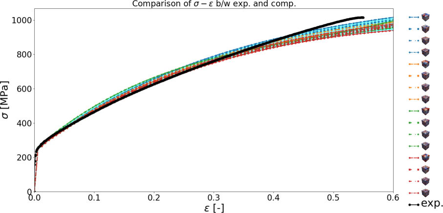
Figure 7: Comparison of homogenized materials properties between experimental data and computational results for SS304L across different mesh resolutions and for different SERVEs.

The fourth aspect addresses an effort in calibrating constitutive model in a high-throughput and asynchronous parallel manner, using one of our previous work [34, 35, 36]. In this section, we focus on the optimization under (microstructure-induced, also known as aleatory) uncertainty with applications to constitutive model calibration. The loss function to be minimized is measured in $\displaystyle L_{2}$-norm and normalized by the maximum observable equivalent strain $\displaystyle\varepsilon_{\text{vM}}$. A set of five constitutive parameters is used to parametrize a phenomenological constitutive model for stainless steel 304L. At any time, 12 CPFEM simulations are performed concurrently, where the batch configuration is set as (8,4,0). To account for the aleatory uncertainty, we average the loss function over an ensemble of 5 SERVEs, where the mesh of $\displaystyle 5\times 5\times 5$ is used.

Figure 7 shows the comparison between the computational results produced by the optimal 5d constitutive parameters and the experimental data (marked as solid black line). The aleatory uncertainty is colored in a cyan shaded region (readers are referred to the color version online). Figure 7 shows a good agreement between experimental data and computational results up to approximately $\displaystyle\varepsilon\approx 0.42$ of strain, which is considerable for CPFEM. The optimal constitutive parameters is found after 352 iterations using the aphBO-2GP-3B algorithm [34].

6 Solving stochastic inverse in property-structure relationship with ML

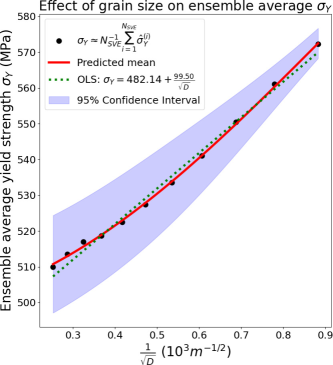
(a) Hall-Petch relationship by ordinary least square and Gaussian process regression.

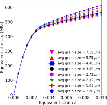
(b) Equivalent stress-strain curve for different average grain sizes.

Figure 8: Figure 8(a): The inferred ML Hall-Petch relationship with 95% confidence intervals for a TWIP steel, and a comparison with a least squares regression model. Figure 8(b): The representative equivalent stress-strain relationship with respect to various average grain sizes. CPFEM simulations are performed with $\displaystyle 64\mu m\times 64\mu m\times 64\mu m$ SVE at the loading condition of $\displaystyle\dot{\varepsilon}_{11}=0.001\text{s}^{-1}$. (Reprinted with permission from [37] ©2020 The Minerals, Metals & Materials Society.)

The last aspect [37] applies a stochastic inverse UQ methodology [38, 39, 40] to infer a data-consistent distribution of microstructure features, in the sense that the push-forward distribution through CPFEM matches the target distribution of the homogenized materials properties of interests. In this case study, we employed a dislocation-density-based for twinning-induced plasticity/transformation-induced plasticity (TWIP/TRIP) Fe-22Mn-0.6C steels [41], where the density of average grain size is inferred based on a ML surrogate (i.e. a heteroscedastic Gaussian process regression) for the Hall-Petch relationship to match target distribution of yield stress. The caveat in this case study is the notion of heteroscedastic behavior under a fixed size assumption of SERVE. Let $\displaystyle D$ denotes the average grain size. When the average grain size $\displaystyle D$ increases, the average grain volume scales as $\displaystyle\mathcal{O}(D^{3})$, and under the assumption of fixed volume for SERVEs, the number of grain size $\displaystyle n$ decreases as $\displaystyle n\sim\mathcal{O}(D^{-3})$. The variance of the Monte Carlo estimator scales as $\displaystyle n^{-1}\sim\mathcal{O}(D^{3})$. Hence larger average grain size would induce a larger variance in the Monte Carlo estimator. As such, the regression is heteroscedastic.

Figure 8(a) shows the Hall-Petch relationship obtained from CPFEM, estimated by the posterior mean of the heteroscedastic Gaussian process regression ( ) and ordinary least square ( ). The ensemble average observations are denoted as $\displaystyle\mathbin{\vbox{\hbox{\scalebox{0.75}{$\displaystyle\bullet$}}}}$. Figure 8(b) shows the equivalent stress-strain curve for different average grain size at the initial yield 0.2% offset.

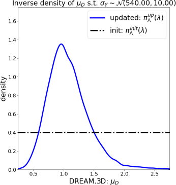
(a) Uniform initial density $\displaystyle\pi_{\mathbf{\Lambda}}^{\text{init}}(\lambda)=\mathcal{U}(0.25,2.75)$ and updated density $\displaystyle\pi_{\mathbf{\Lambda}}^{\text{up}}(\lambda)$ where $\displaystyle\lambda=\mu_{D}$.

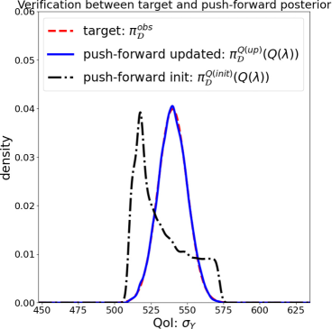
(b) Target $\displaystyle\pi_{\mathbf{\mathcal{D}}}^{\text{obs}}=\mathcal{N}(540,10)$ and push-forward of the updated density $\displaystyle\pi_{\mathbf{\Lambda}}^{\text{up}}(Q(\lambda))$.

Figure 9: Figure 9(a): The initial density, $\displaystyle\pi_{\mathbf{\Lambda}}^{\text{init}}(\lambda)=\mathcal{U}(0.25,2.75)$, and updated density, $\displaystyle\pi_{\mathbf{\Lambda}}^{\text{up}}(\lambda)$, on the microstructure feature $\displaystyle\lambda=\mu_{D}$. Figure 9(b): The target density on material properties, $\displaystyle\pi_{\mathbf{\mathcal{D}}}^{\text{obs}}=\mathcal{N}(540,10)$, and push-forwards of the initial and updated densities. (Reprinted with permission from [37] ©2020 The Minerals, Metals & Materials Society.)

Figure 9(a) shows the uniform prior and the posterior distributions of average grain size, where the posterior is updated using the stochastic inverse method. Figure 9(b) shows the normal target distribution $\displaystyle\mathcal{N}(540,10)$, the push-forward of the prior, and the push-forward of the posterior. The push-forward of the posterior and the target distribution of the yield stress agrees very well with each other.

7 Discussion & Conclusion

In this paper, we survey our recent or on-going research effort in UQ, optimization, and ML for structure-property relationship using CPFEM. As the microstructure is usually high-dimensional and naturally random, deploying UQ techniques is necessary to conduct an efficient and effective numerical studies. In this paper, we demonstrate multiple aspects of using UQ mathematical methodologies in the interest of CPFEM for structure-property relationship. Even though the field of UQ and multiscale computational materials science both have been found for a relatively long time, there is still plenty of research opportunities and open questions for further research. The objective of this paper is to highlight a few interesting and contemporary topics in UQ for CPFEM.

References

- de Pablo et al. [2019] de Pablo, J. J., Jackson, N. E., Webb, M. A., Chen, L.-Q., Moore, J. E., Morgan, D., Jacobs, R., Pollock, T., Schlom, D. G., Toberer, E. S., et al., “New frontiers for the materials genome initiative,” npj Computational Materials, Vol. 5, No. 1, 2019, pp. 1–23.
- Oden et al. [2010a] Oden, T., Moser, R., and Ghattas, O., “Computer predictions with quantified uncertainty, Part I,” SIAM News, Vol. 43, No. 9, 2010a, pp. 1–3.
- Oden et al. [2010b] Oden, T., Moser, R., and Ghattas, O., “Computer predictions with quantified uncertainty, Part II,” SIAM News, Vol. 43, No. 10, 2010b, pp. 1–4.
- Groeber and Jackson [2014] Groeber, M. A., and Jackson, M. A., “DREAM.3D: a digital representation environment for the analysis of microstructure in 3D,” Integrating materials and manufacturing innovation, Vol. 3, No. 1, 2014, p. 5.
- Roters et al. [2012] Roters, F., Eisenlohr, P., Kords, C., Tjahjanto, D., Diehl, M., and Raabe, D., “DAMASK: the Düsseldorf Advanced MAterial Simulation Kit for studying crystal plasticity using an FE based or a spectral numerical solver,” Procedia Iutam, Vol. 3, 2012, pp. 3–10.
- Roters et al. [2019] Roters, F., Diehl, M., Shanthraj, P., Eisenlohr, P., Reuber, C., Wong, S. L., Maiti, T., Ebrahimi, A., Hochrainer, T., Fabritius, H.-O., et al., “DAMASK–The Düsseldorf Advanced Material Simulation Kit for modeling multi-physics crystal plasticity, thermal, and damage phenomena from the single crystal up to the component scale,” Computational Materials Science, Vol. 158, 2019, pp. 420–478.
- Diehl et al. [2017] Diehl, M., Groeber, M., Haase, C., Molodov, D. A., Roters, F., and Raabe, D., “Identifying structure–property relationships through DREAM.3D representative volume elements and DAMASK crystal plasticity simulations: An integrated computational materials engineering approach,” JOM, Vol. 69, No. 5, 2017, pp. 848–855.
- Tran et al. [2022a] Tran, A., Wildey, T., and Lim, H., “Microstructure-sensitive uncertainty quantification for crystal plasticity finite element constitutive models using stochastic collocation method,” Frontiers in Materials, Vol. 9, 2022a, pp. 1–20.
- Xiu and Karniadakis [2002] Xiu, D., and Karniadakis, G. E., “The Wiener–Askey polynomial chaos for stochastic differential equations,” SIAM Journal on Scientific Computing, Vol. 24, No. 2, 2002, pp. 619–644.
- Babuška et al. [2007] Babuška, I., Nobile, F., and Tempone, R., “A stochastic collocation method for elliptic partial differential equations with random input data,” SIAM Journal on Numerical Analysis, Vol. 45, No. 3, 2007, pp. 1005–1034.
- Nobile et al. [2008] Nobile, F., Tempone, R., and Webster, C. G., “A sparse grid stochastic collocation method for partial differential equations with random input data,” SIAM Journal on Numerical Analysis, Vol. 46, No. 5, 2008, pp. 2309–2345.
- Xiu [2009] Xiu, D., “Fast numerical methods for stochastic computations: a review,” Communications in computational physics, Vol. 5, No. 2-4, 2009, pp. 242–272.
- Novak and Ritter [1996] Novak, E., and Ritter, K., “High dimensional integration of smooth functions over cubes,” Numerische Mathematik, Vol. 75, No. 1, 1996, pp. 79–97.
- Novak and Ritter [1997] Novak, E., and Ritter, K., “The curse of dimension and a universal method for numerical integration,” Multivariate approximation and splines, Springer, 1997, pp. 177–187.
- Novak and Ritter [1999] Novak, E., and Ritter, K., “Simple cubature formulas with high polynomial exactness,” Constructive approximation, Vol. 15, No. 4, 1999, pp. 499–522.
- Barthelmann et al. [2000] Barthelmann, V., Novak, E., and Ritter, K., “High dimensional polynomial interpolation on sparse grids,” Advances in Computational Mathematics, Vol. 12, No. 4, 2000, pp. 273–288.
- Sudret [2008] Sudret, B., “Global sensitivity analysis using polynomial chaos expansions,” Reliability engineering & system safety, Vol. 93, No. 7, 2008, pp. 964–979.
- Crestaux et al. [2009] Crestaux, T., Le Maıtre, O., and Martinez, J.-M., “Polynomial chaos expansion for sensitivity analysis,” Reliability Engineering & System Safety, Vol. 94, No. 7, 2009, pp. 1161–1172.
- Saltelli et al. [2010] Saltelli, A., Annoni, P., Azzini, I., Campolongo, F., Ratto, M., and Tarantola, S., “Variance based sensitivity analysis of model output. Design and estimator for the total sensitivity index,” Computer physics communications, Vol. 181, No. 2, 2010, pp. 259–270.
- Tang et al. [2010] Tang, G., Iaccarino, G., and Eldred, M., “Global sensitivity analysis for stochastic collocation,” 51st AIAA/ASME/ASCE/AHS/ASC Structures, Structural Dynamics, and Materials Conference 18th AIAA/ASME/AHS Adaptive Structures Conference 12th, 2010, p. 2922.
- Giles [2008] Giles, M. B., “Multilevel Monte Carlo path simulation,” Operations research, Vol. 56, No. 3, 2008, pp. 607–617.
- Giles [2015] Giles, M. B., “Multilevel Monte Carlo methods,” Acta Numerica, Vol. 24, 2015, pp. 259–328.
- Haji-Ali et al. [2016a] Haji-Ali, A.-L., Nobile, F., and Tempone, R., “Multi-index Monte Carlo: when sparsity meets sampling,” Numerische Mathematik, Vol. 132, No. 4, 2016a, pp. 767–806.
- Haji-Ali et al. [2016b] Haji-Ali, A.-L., Nobile, F., Tamellini, L., and Tempone, R., “Multi-index stochastic collocation for random PDEs,” Computer Methods in Applied Mechanics and Engineering, Vol. 306, 2016b, pp. 95–122.
- Haji-Ali et al. [2016c] Haji-Ali, A.-L., Nobile, F., Tamellini, L., and Tempone, R., “Multi-index stochastic collocation convergence rates for random PDEs with parametric regularity,” Foundations of Computational Mathematics, Vol. 16, No. 6, 2016c, pp. 1555–1605.
- Benner et al. [2015] Benner, P., Gugercin, S., and Willcox, K., “A survey of projection-based model reduction methods for parametric dynamical systems,” SIAM review, Vol. 57, No. 4, 2015, pp. 483–531.
- Sirovich [1987] Sirovich, L., “Turbulence and the dynamics of coherent structures. I. Coherent structures,” Quarterly of applied mathematics, Vol. 45, No. 3, 1987, pp. 561–571.
- Bunge [2013] Bunge, H.-J., Texture analysis in materials science: mathematical methods, Elsevier, 2013.
- Kalidindi [2015] Kalidindi, S. R., Hierarchical materials informatics: novel analytics for materials data, Elsevier, 2015.
- Golub and Van Loan [2013] Golub, G. H., and Van Loan, C. F., Matrix computations, Johns Hopkins University Press, 2013.
- Berkooz et al. [1993] Berkooz, G., Holmes, P., and Lumley, J. L., “The proper orthogonal decomposition in the analysis of turbulent flows,” Annual review of fluid mechanics, Vol. 25, No. 1, 1993, pp. 539–575.
- Bui-Thanh et al. [2008] Bui-Thanh, T., Willcox, K., and Ghattas, O., “Model reduction for large-scale systems with high-dimensional parametric input space,” SIAM Journal on Scientific Computing, Vol. 30, No. 6, 2008, pp. 3270–3288.
- Carlberg et al. [2017] Carlberg, K., Barone, M., and Antil, H., “Galerkin v. least-squares Petrov–Galerkin projection in nonlinear model reduction,” Journal of Computational Physics, Vol. 330, 2017, pp. 693–734.
- Tran et al. [2022b] Tran, A., Eldred, M., Wildey, T., McCann, S., Sun, J., and Visintainer, R. J., “aphBO-2GP-3B: a budgeted asynchronous parallel multi-acquisition functions for constrained Bayesian optimization on high-performing computing architecture,” Structural and Multidisciplinary Optimization, Vol. 65, No. 4, 2022b, pp. 1–45.
- Tran et al. [2019] Tran, A., Sun, J., Furlan, J. M., Pagalthivarthi, K. V., Visintainer, R. J., and Wang, Y., “pBO-2GP-3B: A batch parallel known/unknown constrained Bayesian optimization with feasibility classification and its applications in computational fluid dynamics,” Computer Methods in Applied Mechanics and Engineering, Vol. 347, 2019, pp. 827–852.
- Tran et al. [2020] Tran, A., Tranchida, J., Wildey, T., and Thompson, A. P., “Multi-fidelity machine-learning with uncertainty quantification and Bayesian optimization for materials design: Application to ternary random alloys,” The Journal of Chemical Physics, Vol. 153, 2020, p. 074705.
- Tran and Wildey [2020] Tran, A., and Wildey, T., “Solving stochastic inverse problems for property-structure linkages using data-consistent inversion and machine learning,” JOM, Vol. 73, 2020, pp. 72–89.
- Butler et al. [2018a] Butler, T., Jakeman, J., and Wildey, T., “Convergence of Probability Densities Using Approximate Models for Forward and Inverse Problems in Uncertainty Quantification,” SIAM Journal on Scientific Computing, Vol. 40, No. 5, 2018a, pp. A3523–A3548.
- Butler et al. [2018b] Butler, T., Jakeman, J., and Wildey, T., “Combining push-forward measures and Bayes’ rule to construct consistent solutions to stochastic inverse problems,” SIAM Journal on Scientific Computing, Vol. 40, No. 2, 2018b, pp. A984–A1011.
- Butler et al. [2020] Butler, T., Wildey, T., and Yen, T. Y., “Data-consistent inversion for stochastic input-to-output maps,” Inverse Problems, 2020.
- Wong et al. [2016] Wong, S. L., Madivala, M., Prahl, U., Roters, F., and Raabe, D., “A crystal plasticity model for twinning-and transformation-induced plasticity,” Acta Materialia, Vol. 118, 2016, pp. 140–151.