AutoHyper: Explicit-State Model
Checking for HyperLTL

Abstract

HyperLTL is a temporal logic that can express hyperproperties, i.e., properties that relate multiple execution traces of a system. Such properties are becoming increasingly important and naturally occur, e.g., in information-flow control, robustness, mutation testing, path planning, and causality checking. Thus far, complete model checking tools for HyperLTL have been limited to alternation-free formulas, i.e., formulas that use only universal or only existential trace quantification. Properties involving quantifier alternations could only be handled in an incomplete way, i.e., the verification might fail even though the property holds. In this paper, we present AutoHyper, an explicit-state automata-based model checker that supports full HyperLTL and is complete for properties with arbitrary quantifier alternations. We show that language inclusion checks can be integrated into HyperLTL verification, which allows AutoHyper to benefit from a range of existing inclusion-checking tools. We evaluate AutoHyper on a broad set of benchmarks drawn from different areas in the literature and compare it with existing (incomplete) methods for HyperLTL verification.

1 Introduction

Hyperproperties [15] are system properties that relate multiple executions of a system. Such properties are of increasing importance as they naturally occur, e.g., in information-flow control [35], robustness [21], linearizability [29, 30], path planning [38], mutation testing [26], and causality checking [17]. A prominent logic to express hyperproperties is HyperLTL, which extends linear-time temporal logic (LTL) with explicit trace quantification [14]. HyperLTL can, for instance, express generalized non-interference (GNI) [33], stating that the high-security input of a system does not influence the observable output.

$$\forall\pi\mathpunct{.}\forall\pi^{\prime}\mathpunct{.}\exists\pi^{\prime\prime}\mathpunct{.}\operatorname{\leavevmode\hbox to6.97pt{\vbox to6.97pt{\text{[drawing]}}}}\Big{(}\bigwedge_{a\in H}a_{\pi}\leftrightarrow a_{\pi^{\prime\prime}}\Big{)}\land\operatorname{\leavevmode\hbox to6.97pt{\vbox to6.97pt{\text{[drawing]}}}}\Big{(}\bigwedge_{a\in L\cup O}a_{\pi^{\prime}}\leftrightarrow a_{\pi^{\prime\prime}}\Big{)}$$ (GNI)

Here, $H$ is a set of high-security input, $L$ is a set of low-security inputs, and $O$ is a set of low-security outputs. The formula states that for any traces $\pi,\pi^{\prime}$ there exists a third trace $\pi^{\prime\prime}$ that agrees with the high-security inputs of $\pi$ and with the low-security inputs and outputs of $\pi^{\prime}$. Any observation made by a low-security attacker is thus compatible with every possible high-security input.

We are interested in the model checking (MC) problem of HyperLTL, i.e., whether a given (finite-state) system satisfies a given property. For HyperLTL, the structure of the quantifier prefix directly impacts the complexity of this problem. For alternation-free formulas (i.e., formulas that only use quantifiers of a single type), verification is well understood and is reducible to the verification of a trace property on a self-composition of the system [3]. This reduction has, for example, been implemented in MCHyper [28], a tool that can model check (alternation-free) HyperLTL formulas in systems of considerable size (circuits with thousands of latches).

Verification is much more challenging for properties involving quantifier alternations (such as GNI from above). While MC algorithms supporting full HyperLTL exist (see [14, 28]), they have not been implemented yet. Instead, over the years, a number of approaches to the verification of such properties in practice have been made: Finkbeiner et al. [28] and D’Argenio et al. [21] manually strengthen properties with quantifier alternation into properties that are alternation-free and can be checked by MCHyper. Coenen et al. [18] instantiate existential quantification in a $\forall^{*}\exists^{*}$ property (i.e., a property involving an arbitrary number of universal quantifiers followed by an arbitrary number of existential quantifiers, such as GNI) with an explicit (user-provided) strategy, thus reducing to the verification of an alternation-free formula. Alternatively, the strategy that resolves existential quantification can be automatically synthesized [8]. Hsu et al. [30] present a bounded model checking (BMC) approach for HyperLTL that is implemented in HyperQube. See Section 4 for more details.

While all these verification tools can verify (or refute) interesting properties, they all suffer from the same fundamental limitation: they are incomplete. That is, for all the tools above, we can come up with verification instances where they fail, not because of resource constraints but because of inherent limitations in the underlying verification algorithm. Moreover, such instances are not rare events but are encountered regularly in practice. For example, many of the benchmarks used to evaluate HyperQube (by Hsu et al. [30]) do not admit a strategy to resolve existential quantification. Conversely, many of the properties verified by Coenen et al. [18] (such as GNI) cannot be verified using BMC [30].

AutoHyper.

In this paper, we present AutoHyper, a model checker for HyperLTL. Our tool checks a hyperproperty by iteratively eliminating trace quantification using automata-complementations, thereby reducing verification to the emptiness check of an automaton [28]. Importantly – and different from previous tools for HyperLTL verification such as MCHyper [28, 18] and HyperQube [30] – AutoHyper can cope with (and is complete for) arbitrary HyperLTL formulas. Model checking using AutoHyper does not require manual effort (such as writing an explicit strategy in MCHyper [18]), nor does a user need to worry if the given property can even be verified with a given method. AutoHyper thus provides a “push-button” model checking experience for HyperLTL.

To improve AutoHyper’s efficiency, we make the (theoretical) observation that we can often avoid explicit automaton complementation and instead reduce to a language inclusion check on Büchi automata (cf. Proposition 1). On the practical side, this enables AutoHyper to resort to a range of mature language inclusion checkers, including spot [25], RABIT [16], BAIT [24], and FORKLIFT [23].

Evaluation.

Using AutoHyper, we extensively study the practical aspects of model checking HyperLTL properties with quantifier alternations. To evaluate the performance of explicit-state model checking, we apply AutoHyper to a broad range of benchmarks taken from the literature and compare it with existing (incomplete) tools. We make the surprising observation that – at least on the currently available benchmarks – explicit-state MC as implemented in AutoHyper performs on-par (and frequently outperforms) symbolic methods such as BMC [30]. Our benchmarks stem from various areas within computer science, so AutoHyper should – thanks to its “push-button” functionality, completeness, and ease of use – be a valuable addition to many areas.

Apart from using AutoHyper as a practical MC tool, we can also use it as a complete baseline to systematically evaluate existing (incomplete) methods. For example, while it is known that replacing existential quantification with a strategy (as done by Coenen et al. [18]) is incomplete, it was, thus far, unknown if this incompleteness occurs frequently or is merely a rare phenomenon. We use AutoHyper to obtain a ground truth and evaluate the strategy-based verification approach in terms of its effectiveness (i.e., how many instances it can verify despite being incomplete) and efficiency.

Structure.

The remainder of this paper is structured as follows. In Section 2, we introduce HyperLTL. We recap automaton-based verification (which we abbreviate ABV) and our new approach utilizing language inclusion checks in Section 3. We discuss alternative verification approaches for HyperLTL in Section 4. In Section 6, we compare different backend solving techniques and study the complexity of HyperLTL MC with multiple quantifier alternations in practice; In Section 7, we evaluate ABV on a set of benchmarks from the literature and compare with the bounded model checker HyperQube [30]; In Section 8 we use AutoHyper for a detailed analysis of (and comparison with) strategy-based verification [18, 8].

2 Preliminaries

We fix a set of atomic propositions $\mathit{AP}$ and define $\Sigma:=2^{\mathit{AP}}$. HyperLTL [14] extends LTL with explicit quantification over traces, thereby lifting it from a logic expressing trace properties to one expressing hyperproperties [15]. Let $\mathcal{V}$ be a set of trace variables. We define HyperLTL formulas by the following grammar:

$$\psi :=a_{\pi}\mid\neg\psi\mid\psi\land\psi\mid\operatorname{\leavevmode\hbox to7.41pt{\vbox to7.41pt{\text{[drawing]}}}}\psi\mid\psi\operatorname{\mathcal{U}}\psi$$

$$\varphi :=\exists\pi\mathpunct{.}\varphi\mid\forall\pi\mathpunct{.}\varphi\mid\psi$$

where $\pi\in\mathcal{V}$ and $a\in\mathit{AP}$.

We assume that the formula is closed, i.e., all trace variables that are used in the body are bound by some quantifier. The semantics of HyperLTL is given with respect to a trace assignment $\Pi:\mathcal{V}\rightharpoonup\Sigma^{\omega}$ mapping trace variables to traces. For $\pi\in\mathcal{V}$ and $t\in\Sigma^{\omega}$, we write $\Pi[\pi\mapsto t]$ for the trace assignment obtained by updating the value of $\pi$ to $t$. Given a set of traces $\mathbb{T}\subseteq\Sigma^{\omega}$, a trace assignment $\Pi$, and $i\in\mathbb{N}$, we define:

$$\Pi,i \models a_{\pi} a\in\Pi(\pi)(i)$$ iff

$$\Pi,i \models\neg\psi \Pi,i\not\models\psi$$ iff

$$\Pi,i \models\psi_{1}\land\psi_{2} \Pi,i\models\psi_{1}\text{ and }\Pi,i\models\psi_{2}$$ iff

$$\Pi,i \models\operatorname{\leavevmode\hbox to7.41pt{\vbox to7.41pt{\text{[drawing]}}}}\psi \Pi,i+1\models\psi$$ iff

$$\Pi,i \models\psi_{1}\operatorname{\mathcal{U}}\psi_{2} \exists j\geq i\mathpunct{.}\Pi,j\models\psi_{2}\text{ and }\forall i\leq k<j\mathpunct{.}\Pi,k\models\psi_{1}$$ iff

$$\Pi \models_{\mathbb{T}}\psi \Pi,0\models\psi$$ iff

$$\Pi \models_{\mathbb{T}}\exists\pi\mathpunct{.}\varphi \exists t\in\mathbb{T}\mathpunct{.}\Pi[\pi\mapsto t]\models_{\mathbb{T}}\varphi$$ iff

$$\Pi \models_{\mathbb{T}}\forall\pi\mathpunct{.}\varphi \forall t\in\mathbb{T}\mathpunct{.}\Pi[\pi\mapsto t]\models_{\mathbb{T}}\varphi$$ iff

A transition system is a tuple $\mathcal{T}=(S,S_{0},\kappa,L)$ where $S$ is a set of states, $S_{0}\subseteq S$ is a set of initial states, $\kappa\subseteq S\times S$ is a transition relation, and $L:S\to\Sigma$ is a labeling function. We write $s\mathrel{\raisebox{-1.0pt}{$\xrightarrow{\mathcal{T}}$}}s^{\prime}$ whenever $(s,s^{\prime})\in\kappa$. A path is an infinite sequence $s_{0}s_{1}s_{2}\cdots\in S^{\omega}$, s.t., $s_{0}\in S_{0}$, and $s_{i}\mathrel{\raisebox{-1.0pt}{$\xrightarrow{\mathcal{T}}$}}s_{i+1}$ for all $i$. The associated trace is given by $L(s_{0})L(s_{1})L(s_{2})\cdots\in\Sigma^{\omega}$. We write $\mathit{Traces}(\mathcal{T})\subseteq\Sigma^{\omega}$ for the set of all traces generated by $\mathcal{T}$. We say $\mathcal{T}$ satisfies a HyperLTL property $\varphi$, written $\mathcal{T}\models\varphi$, if $\emptyset\models_{\mathit{Traces}(\mathcal{T})}\varphi$, where $\emptyset$ denotes the empty trace assignment.

3 Automata-based HyperLTL Model Checking

Given a system $\mathcal{T}$ and HyperLTL property $\varphi$, we want to decide whether $\mathcal{T}\models\varphi$. In this section, we recap the automaton-based approach to the model checking of HyperLTL [28]. We further show how language inclusion checks can be incorporated into the model checking procedure to make use of a broad collection of mature language inclusion checkers.

3.1 Automata-based Verification

The idea of automata-based verification (ABV) [28] is to iteratively eliminate quantifiers and thus reduce MC to the emptiness check on an automaton. A non-deterministic Büchi automaton (NBA) is a tuple $\mathcal{A}=(Q,Q_{0},\delta,F)$ where $Q$ is a finite set of states, $Q_{0}\subseteq Q$ is a set of initial states, $\delta:Q\times\Sigma\to 2^{Q}$ is a transition function, and $F\subseteq Q$ is a set of accepting states. We write $\mathcal{L}(\mathcal{A})\subseteq\Sigma^{\omega}$ for the language of $\mathcal{A}$, i.e., all infinite words that have a run that visits states in $F$ infinitely many times (see, e.g., [2]). For traces $t_{1},\ldots,t_{n}\in\Sigma^{\omega}$, we write $\mathit{zip}(t_{1},\ldots,t_{n})\in(\Sigma^{n})^{\omega}$ as the pointwise product, i.e., $\mathit{zip}(t_{1},\ldots,t_{n})(i):=(t_{1}(i),\ldots,t_{n}(i))$.

Let $\mathcal{T}=(S,S_{0},\kappa,L)$ be a fixed transition system and let $\dot{\varphi}$ be some fixed closed HyperLTL formula (we use the dot to refer to the original formula and use $\varphi,\varphi^{\prime}$ to refer to subformulas of $\dot{\varphi}$). For some subformula $\varphi$ that contains free trace variables $\pi_{1},\ldots,\pi_{n}$, we say an NBA $\mathcal{A}$ over $\Sigma^{n}$ is $\mathcal{T}$-equivalent to $\varphi$, if for all traces $t_{1},\ldots,t_{n}$ it holds that $[\pi_{1}\mapsto t_{1},\ldots,\pi_{n}\mapsto t_{n}]\models_{\mathit{Traces}(\mathcal{T})}\varphi$ iff $\mathit{zip}(t_{1},\ldots,t_{n})\in\mathcal{L}(\mathcal{A})$. That is, $\mathcal{A}$ accepts exactly the zippings of traces that constitute a satisfying trace assignment for $\varphi$.

To check if $\mathcal{T}\models\dot{\varphi}$, we inductively construct an automation $\mathcal{A}_{\varphi}$ that is $\mathcal{T}$-equivalent to $\varphi$ for each subformula $\varphi$ of $\dot{\varphi}$. For the (quantifier-free) LTL body of $\dot{\varphi}$, we can construct this automaton via a standard LTL-to-NBA construction [28, 2]. Now consider some subformula $\varphi^{\prime}=\exists\pi.\varphi$ where $\varphi^{\prime}$ contains free trace variables $\pi_{1},\ldots,\pi_{n}$ and so $\varphi$ contains free trace variables $\pi_{1},\ldots,\pi_{n},\pi$. We are given an inductively constructed NBA $\mathcal{A}_{\varphi}=(Q,Q_{0},\delta,F)$ over $\Sigma^{n+1}$ that is $\mathcal{T}$-equivalent to $\varphi$. We define the automaton $\mathcal{A}_{\varphi^{\prime}}$ over $\Sigma^{n}$ as $\mathcal{A}_{\varphi^{\prime}}:=(S\times Q,S_{0}\times Q_{0},\delta^{\prime},S\times F)$ where $\delta^{\prime}$ is defined as

$$\delta^{\prime}\Big{(}(s,q),\big{\langle}l_{1},\ldots,l_{n}\big{\rangle}\Big{)}:=\Big{\{}(s^{\prime},q^{\prime})\mid s\xrightarrow{\mathcal{T}}s^{\prime}\;\land\;q^{\prime}\in\delta\big{(}q,\big{\langle}l_{1},\ldots,l_{n},L(s)\big{\rangle}\big{)}\Big{\}}.$$

Informally, $\mathcal{A}_{\varphi^{\prime}}$ reads the zippings of traces $t_{1},\ldots,t_{n}$ and guesses a trace $t\in\mathit{Traces}(\mathcal{T})$ such that $\mathit{zip}(t_{1},\ldots,t_{n},t)\in\mathcal{L}(\mathcal{A}_{\varphi})$. It is easy to see that $\mathcal{A}_{\varphi^{\prime}}$ is $\mathcal{T}$-equivalent to $\varphi^{\prime}$. To handle universal trace quantification, we consider a formula $\varphi^{\prime}=\forall\pi.\varphi$ as $\varphi^{\prime}=\neg\exists\pi.\neg\varphi$ and combine the construction for existential quantification with an automaton complementation.

Following the inductive construction, we obtain an automaton $\mathcal{A}_{\dot{\varphi}}$ over the singleton alphabet $\Sigma^{0}$ that is $\mathcal{T}$-equivalent to $\dot{\varphi}$. By definition of $\mathcal{T}$-equivalence, $\mathcal{T}\models{\dot{\varphi}}$ iff $\emptyset\models_{\mathit{Traces}(\mathcal{T})}\dot{\varphi}$ iff $\mathcal{A}_{\dot{\varphi}}$ is non-empty (which we can decide [20]).

3.2 HyperLTL Model Checking by Language Inclusion

The algorithm outlined above requires one complementation for each quantifier alternation in the HyperLTL formula. While we cannot avoid the theoretical cost of this complementation (see [35, 14]), we can reduce to a, in practice, more tamable problem: language inclusion.

For a system $\mathcal{T}$, and a natural number $n\in\mathbb{N}$ we define $\mathcal{A}_{\mathcal{T}}^{n}$ as an NBA over $\Sigma^{n}$ such that for any traces $t_{1},\ldots,t_{n}\in\Sigma^{\omega}$ we have $\mathit{zip}(t_{1},\ldots,t_{n})\in\mathcal{L}(\mathcal{A}_{\mathcal{T}}^{n})$ if and only if $t_{i}\in\mathit{Traces}(\mathcal{T})$ for every $1\leq i\leq n$. We can construct $\mathcal{A}_{\mathcal{T}}^{n}$ by building the $n$-fold self-composition of $\mathcal{T}$ [3] and convert this to an automaton by moving the labels from states to edges and marking all states as accepting. We can now state a formal connection between language inclusion and HyperLTL MC (a proof can be found in Appendix 0.A):

Proposition 1 ()

Let $\dot{\varphi}=\forall\pi_{1}.\ldots\forall\pi_{n}.\varphi$ be a HyperLTL formula (where $\varphi$ may contain additional trace quantifiers) and let $\mathcal{A}_{\varphi}$ be an automaton over $\Sigma^{n}$ that is $\mathcal{T}$-equivalent to $\varphi$. Then $\mathcal{T}\models\dot{\varphi}$ if and only if $\mathcal{L}(\mathcal{A}_{\mathcal{T}}^{n})\subseteq\mathcal{L}(\mathcal{A}_{\varphi})$.

We can use Proposition 1 to avoid a complementation for the outermost quantifier alternation. For example, assume $\dot{\varphi}=\forall\pi_{1}.\forall\pi_{2}.\exists\pi_{3}.\psi$ where $\psi$ is quantifier-free. Using the construction from Section 3.1, we obtain an automaton $\mathcal{A}_{\exists\pi_{3}.\psi}$ that is $\mathcal{T}$-equivalent to $\exists\pi_{3}.\psi$ (we can construct $\mathcal{A}_{\exists\pi_{3}.\psi}$ in linear time in the size of $\mathcal{T}$). By Proposition 1, we then have $\mathcal{T}\models\dot{\varphi}$ iff $\mathcal{L}(\mathcal{A}^{2}_{\mathcal{T}})\subseteq\mathcal{L}(\mathcal{A}_{\exists\pi_{3}.\psi})$.

Note that complementation and subsequent emptiness check is a theoretically optimal method to solve the (PSPACE-complete) language inclusion problem. Proposition 1 thus offers no asymptotic advantages over “standard” ABV in Section 3.1. In practice constructing an explicit complemented automaton is often unnecessary as the language inclusion or non-inclusion might be witnessed without a complete complementation [25, 24, 16, 23]. This makes Proposition 1 relevant for the present work and the performance of AutoHyper.

4 Related Work and HyperLTL Verification Approaches

HyperLTL [14] is the most studied logic for expressing hyperproperties. A range of problems from different areas in computer science can be expressed as HyperLTL MC problems, including (optimal) path panning [38], mutation testing [26], linearizability [30], robustness [21], information-flow control [35], and causality checking [17], to name only a few. Consequently, any model checking tool for HyperLTL is applicable to many disciples within computer science and provides a unified solution to many challenging algorithmic problems. In recent years, different (mostly incomplete) methods for the verification of HyperLTL have been developed. We discuss them below (see Appendix 0.B for details).

Automata-based Model Checking.

Finkbeiner et al. [28] introduce the automata-based model checking approach as presented in Section 3.1. For alternation-free formulas, the algorithms corresponds to the construction of the self-composition of a system [3] and is implemented in the MCHyper tool [28]. MCHyper can handle systems of significant size (well beyond the reach of explicit-state methods) but is unable to handle any quantifier alternation (the main motivation for AutoHyper). htltl2mc [14] is a prototype model checker for HyperLTL₂ (a fragment of HyperLTL with at most one alternation) built on top of GOAL [37]. In contrast to htltl2mc, AutoHyper supports properties with arbitrarily many quantifier alternations and features automata with symbolic alphabets – which is important to handle large systems with many atomic propositions, cf. Footnote 7).

Strategy-based Verification.

Coenen et al. [18] verify $\forall^{*}\exists^{*}$ properties by instantiating existential quantification with an explicit strategy. This method – which we refer to as strategy-based verification (SBV) – comes in two flavors: either the strategy is provided by the user or the strategy is synthesized automatically. In the former case, model checking reduces to checking an alternation-free formula and can thus handle large systems, but requires significant user effort (and is thus no “push-button” technique). In the latter case, the method works fully automatically [9, 8] but requires an expensive strategy synthesis. SBV is incomplete as the strategy resolving existentially quantified traces only observes finite prefixes of the universally quantified traces. While SBV can be made complete by adding prophecy variables [8], the automatic synthesis of such prophecies is currently limited to very small systems and properties that are temporally safe [5]. We investigate both the performance and incompleteness of SBV in Section 8.

Bounded Model Checking.

Hsu et al. [30] propose a bounded model checking (BMC) procedure for HyperLTL. Similar to BMC for trace properties [10], the system is unfolded up to a fixed depth, and pending obligations beyond that depth are either treated pessimistically (to show the satisfaction of a formula) or optimistically (to show the violation of a formula). While BMC for trace properties reduces to SAT-solving, BMC for hyperproperties naturally reduces to QBF-solving. As usual for bounded methods, BMC for HyperLTL is incomplete. For example, it can never show that a system satisfies a hyperproperty where the LTL body contains an invariant (as, e.g., is the case for GNI). We compare AutoHyper and BMC (in the form of HyperQube [30]) in Section 7.

5 AutoHyper: Tool Overview

AutoHyper is written in F# and implements the automaton-based verification approach described in Section 3.1 and, if desired by the user, makes use of the language-inclusion-based reduction from Section 3.2. AutoHyper uses spot [25] for LTL-to-NBA translations and automata complementations. To check language inclusion, AutoHyper uses spot (which is based on determinization), RABIT [16] (which is based on a Ramsey-based approach with heavy use of simulations), BAIT [24], and FORKLIFT [23] (both based on well-quasiorders). AutoHyper is designed such that communication with external automata tools is done via established text-based formats (opposed to proprietary APIs), namely the HANOI [1] and BA automaton formats. New (or updated) tools that improve on fundamental automata operations, such as complementation and inclusion checks, can thus be integrated easily. Internally we represent automata using symbolic alphabets (similar to spot). We store transition formulas as DNFs as this allows for very efficient SAT checks, which are needed during the product construction.

All experiments in this paper were conducted on a Mac Mini with an Intel Core i3 (i3-8100B) and 16GB of memory. We used spot version 2.11.1; RABIT version 2.4.5; BAIT commit 369e1a4; and FORKLIFT commit 5d519e3.

Input Formats.

AutoHyper supports both explicit-state systems (given in a HANOI-like [1] input format) and symbolic systems that are internally converted to an explicit-state representation. The support for symbolic systems includes Aiger circuits, symbolic models written in a fragment of the NuSMV input language [12], and a simple boolean programming language [6].

Random Benchmarks.

For our evaluation, we use both existing instances from various sources in the literature and randomly generated problems. We generate random transition systems based on the Erdős–Rényi–Gilbert model [27]. Given a size $n$ and a density parameter $p\in[0,1]$, we generate a graph with $n$ states, where for every two states $s,s^{\prime}$, there is a transition $s\to s^{\prime}$ with probability $p$. To generate a graph with $n$ edges and, in expectation, constant outdegree of $k$, we can choose $p=\tfrac{k}{n}$. We further ensure that the system is connected and all states have at least one outgoing edge. We generate random HyperLTL formulas (with a given quantifier prefix) by sampling the LTL matrix using spot’s randltl.

6 HyperLTL Model Checking Complexity in Practice

Before we turn our attention to benchmarks found in the literature, we compare the different backend inclusion checkers supported by AutoHyper by evaluating them on a large set of synthetic (random) benchmarks (in Section 6.1). Moreover, the random generation of benchmarks allows us to peek at formulas with more than one quantifier alternation. The theoretical hardness of model checking properties with multiple alternations has been studied extensively [14, 35], and we analyze, for the first time, how these results transfer to practice (in Section 6.2).

6.1 Performance of Inclusion Checkers

As the first set of benchmarks, we compare the different backend inclusion checkers supported by AutoHyper. In Figure 1, we depict how many instances can be solved using the inclusion checks of spot, BAIT, RABIT, and FORKLIFT within a timeout of 10s and give the median running time used on the instances that could be solved within the timeout. We observe that spot clearly outperforms RABIT, BAIT, and FORKLIFT in terms of the percentage of instances that can be checked within 10s. While, in general, spot solves the most instances, a manual inspection reveals that there are also instances that can only be solved by RABIT or BAIT/FORKLIFT. This justifies why AutoHyper supports multiple backed inclusion checkers that implement different algorithms and thus excel on different problems (we will confirm this in Section 7). Moreover, our experiments provide evidence that HyperLTL MC is a natural source for challenging language inclusion benchmarks (see Appendix 0.C).

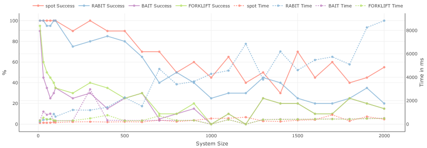
Figure 1: We evaluate different backend solvers on instances of varying system size with an (on average) constant outdegree of 10 and a fixed property size of 20. We generate 20 samples per system size. We display both the success rate of each solver within a timeout of 10s (on the left axis) and the median running time on the solved instances (on the right axis).

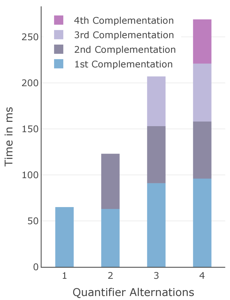
Figure 2: For properties with a varying number of quantifier alterations, we display the average time spent on the automata complementation during model checking.

We remark that we set the timeout of 10s deliberately low to compute (and reproduce) the plots in a reasonable time (computing Figure 1 took about 3.5h). If a user wants to verify a given instance and does not require a result within a few seconds, running the solver for even longer will likely increase the success rate further (see also the evaluation in Section 7).

6.2 Model Checking Beyond $\forall^{*}\exists^{*}$

Using randomly generated benchmarks, we can also peek at the practical complexity of model checking in the presence of multiple quantifier alternations. In theory, the model checking complexity of HyperLTL increases by one exponent with each quantifier alternation [14, 35]. Using AutoHyper, we can, for the first time, investigate the model checking complexity in practice.

We model check randomly generated formulas with $1$ to $4$ quantifier alternations and visualize the total running time based on the cost of each complementation (using spot) in Figure 2 (recall that checking a formula with $k$ alternations using ABV requires $k$ automaton complementations). Although the number of quantifier alternations has an undeniable impact on the total running time (the cumulative height of each bar), the increase in runtime is not proportional to the (non-elementary) increase suggested by the theoretical analysis. Different from the theoretical analysis (where the $(k+1)$th complementation is exponentially more expensive than the $k$th), the cost of each complementation barely increases (or even decreases). This suggests that the $\mathcal{T}$-equivalent automata constructed in each iteration are, in practice, much smaller than indicated by the worst-case theoretical analysis. Verification of properties beyond one alternation is thus less infeasible than the theory suggests (at least on randomly generated test cases).

7 Evaluation on Symbolic Systems

In this section, we challenge AutoHyper with complex model checking problems found in the literature. Our benchmarks stem from a range of sources, including non-interference in boolean programs [6], symmetry in mutual exclusion algorithms [18], non-interference in multi-threaded programs [36], fairness in non-repudiation protocols [31], mutation testing [26], and path planning [38].

7.1 Model Checking GNI on Boolean Programs

Table 1: We depict the running time of AutoHyper when verifying GNI on the boolean programs taken from [6] and [7]. We give the program, the bitwidth (bw), the size of the intermediate explicit-state representation (Size), and the time taken by each solver. The timeout is set to 60s and indicated by a “-”. The property holds in all cases. Times are given in seconds.

Program	bw	Size	$\boldsymbol{t}_{\texttt{spot}}$	$\boldsymbol{t}_{\texttt{RABIT}}$	$\boldsymbol{t}_{\texttt{BAIT}}$	$\boldsymbol{t}_{\texttt{FORKLIFT}}$
[6].1	$1$-bit	17	0.52	0.59	0.80	0.61
	$3$-bit	65	0.56	0.86	-	22.73
	$4$-bit	129	0.99	5.51	-	-
[6].2	$1$-bit	55	0.53	0.69	-	5.49
[6].3	$1$-bit	20	0.52	0.61	3.05	0.98
	$3$-bit	80	0.61	1.31	-	-
[6].4	$1$-bit	29	0.52	0.56	0.58	0.57
	$3$-bit	113	0.67	1.74	-	-

Program	bw	Size	$\boldsymbol{t}_{\texttt{spot}}$	$\boldsymbol{t}_{\texttt{RABIT}}$	$\boldsymbol{t}_{\texttt{BAIT}}$	$\boldsymbol{t}_{\texttt{FORKLIFT}}$
[7].1	$1$-bit	5	0.52	0.56	0.58	0.57
[7].2	$1$-bit	11	0.51	0.57	0.72	0.61
	$2$-bit	27	0.52	0.65	35.7	5.43
	$4$-bit	291	1.46	-	-	-
[7].3	$1$-bit	21	0.52	0.60	3.15	1.00
	$3$-bit	225	-	45.2	-	-
[7].4	$1$-bit	25	0.52	0.71	12.8	1.63
	$3$-bit	193	0.98	-	-	-

We use AutoHyper to verify GNI on a range of boolean programs that process high-security and low-security inputs (taken from [6, 7]). Table 1 depicts the runtime results using different backend solvers. We test each program with varying bitwidth and depict the largest bitwidth that can be solved by at least one solver (within a timeout of 60s). We, again, note that spot performs better than other inclusion checkers and, in particular, scales better when the size of the system increases. Note that the number of atomic propositions is $3$ in all instances, so spot’s support for symbolic alphabets has a negligible impact on the running time. We emphasize that not all instances in Table 1 can be verified using SBV [18, 8] without a user-provided fixed lookahead. Likewise, BMC [30] can never verify GNI. This provides further evidence why complete model checking tools (of which AutoHyper is the first) are necessary.

7.2 Explicit Model Checking of Symbolic Systems

Table 2: We evaluate HyperQube and AutoHyper on the benchmarks from [30]. We list the system and the property (as given in [30, Table 2]), the quantifier structure ($\boldsymbol{Q}^{*}$), the verification result (Res) (✓ indicates that the property holds and ✗ that it is violated), and the total running time of either tool ($t$). For HyperQube, we additionally list the unrolling bound ($k$) and the unrolling semantics (Sem). For AutoHyper, we additionally list the size of the intermediate explicit state space (Size). Times are given in seconds.

				HyperQube [30]			AutoHyper
System	Spec	$\boldsymbol{Q}^{*}$	Res	$\boldsymbol{k}$	Sem ​​​​​	$\boldsymbol{t}$	Size	$\boldsymbol{t}$
Bakery3	$\varphi_{S1}$	$\exists\exists$	✗	7	pes	1.9	167	2.3
Bakery3	$\varphi_{S2}$	$\forall\exists$	✗	12	pes	2.0	167	4.2
Bakery3	$\varphi_{S3}$	$\exists\forall$	✗!	20	pes	2.8	167	34.6
Bakery3	$\varphi_{\mathit{sym}1}$ ​​​​​	$\forall\exists$	✗	10	pes	1.7	167	16.2
Bakery3	$\varphi_{\mathit{sym}2}$​​​​​	$\forall\exists$	✗	10	pes	1.6	167	2.9
Bakery5	$\varphi_{\mathit{sym}1}$ ​​​​​	$\forall\exists$	✗	10	pes	17.3	996	282.1
Bakery5	$\varphi_{\mathit{sym}2}$​​​​​	$\forall\exists$	✗	10	pes	18.2	996	18.0
SNARK-bug1	$\varphi_{\mathit{lin}}$	$\forall\exists$	✗	26	hpes	618.0	4941	96.1
3-Threadcorrect	$\varphi_{\mathit{NI}}$	$\forall\exists$	✓	10	hopt	1.6	64	1.3
3-Threadincorrect	$\varphi_{\mathit{NI}}$	$\forall\exists$	✗	57	hpes	12.8	368	7.7
$\mathit{NRP}:T_{\mathit{correct}}$	$\varphi_{\mathit{fair}}$	$\exists\forall$	✓	15	hopt	1.3	55	0.5
$\mathit{NRP}:T_{\mathit{incorrect}}$	$\varphi_{\mathit{fair}}$	$\exists\forall$	✓!	15	hopt	1.4	54	0.8
$\mathit{Mutant}$	$\varphi_{\mathit{mut}}$	$\exists\forall$	✓	8	hopt	1.1	32	0.8

In this section, we evaluate AutoHyper on challenging symbolic models (NuSMV models [12]) that were used by Hsu et al. [30] to evaluate HyperQube.

The properties we verify cover a wide range of properties. For example, we verify that Lamport’s bakery algorithm [32] does not satisfy various symmetry properties (as the algorithm prioritizes processes with a lower ticket ID); We check linearizability [29] on the SNARK datastructure [22] and identify a previously known bug; And, we generate model-based mutation test cases using the approach proposed by Fellner et al. [26]. Further details on the benchmarks are provided in [30].

We check each instance using both HyperQube and AutoHyper and depict the results in Table 2. When using AutoHyper we always apply spot’s inclusion checker. For HyperQube we use the unrolling semantics and unrolling depth listed in [30, Table 2]. We observe that for most instances – despite using explicit state methods and thus being complete (cf. Section 7.4) – AutoHyper performs on par with HyperQube. On instances using Lamport’s bakery algorithm, BMC only needs to unroll to very shallow depths, resulting in very efficient solving, whereas AutoHyper’s running time is dominated by spot’s LTL-to-NBA translation (consuming up to 98% of the total time). Conversely, on the large SNARK example, AutoHyper performs significantly better.

7.3 Hyperproperties for Path Planning

As a last set of benchmarks, we use planning problems for robots encoded into HyperLTL as proposed by Wang et al. [38]. For example, the synthesis of a shortest path can be phrased as a $\exists\forall$ property that states that there exists a path to the goal such that all alternative paths to the goal take at least as long. Wang et al. [38] propose a solution to check the resulting HyperLTL property by encoding it in first-order logic, which is then solved by an SMT solver. While not competitive with state-of-the-art planning tools, HyperLTL allows one to express a broad range of problems (shortest path, path robustness, etc.) in a very general way. Hsu et al. [30] observe that the QBF encoding implemented in HyperQube outperforms the SMT-based approach by Wang et al. [38]. In this section, we evaluate AutoHyper on these planning-hyperproperties and compare it with HyperQube.

We depict the results in Table 3. It is evident that AutoHyper outperforms HyperQube, sometimes by orders of magnitude. This is surprising as planning problems (which are essentially reachability problems) on symbolic systems should be advantageous for symbolic methods such as BMC. The large size of the intermediate QBF indicates that a more optimized encoding (perhaps specific to path planning) could improve the performance of BMC on such examples.

Table 3: We evaluate HyperQube and AutoHyper on hyperproperties that encode the existence of a shortest path ($\varphi_{\mathit{sp}}$) and robust path ($\varphi_{\mathit{rp}}$). We give the specification (Spec), the size of the grid (Grid), and the times taken by HyperQube and AutoHyper ($t$). For HyperQube, we additionally give the unrolling depth used ($k$) and the file size of the QBF generated (|QBF|). For AutoHyper, we additionally give the size of the generated explicit state space (Size). Times are given in seconds. The timeout is set to 20 min and indicated by a “-”.

		HyperQube [30]			AutoHyper
Spec	Grid	$\boldsymbol{k}$	|QBF|	$\boldsymbol{t}$	Size	$\boldsymbol{t}$
$\varphi_{\mathit{sp}}$	$10\times 10$	20	8 MB	4.6	146	0.68
	$20\times 20$	40	26 MB	168.1	188	1.50
	$40\times 40$	80	-	-	408	22.70
	$60\times 60$	120	-	-	404	88.83
$\varphi_{\mathit{rp}}$	$10\times 10$	20	13 MB	4.2	266	0.59
	$20\times 20$	40	84 MB	22.4	572	0.78
	$40\times 40$	80	419 MB	265	1212	1.58
	$60\times 60$	120	-	-	1852	3.70

7.4 Bounded vs. Explicit-State Model Checking

Bounded model checking has seen remarkable success in the verification of trace properties and frequently scales to systems whose size is well out of scope for explicit-state methods [19]. Similarly, in the context of alternation-free hyperproperties, symbolic verification tools such as MCHyper [28] (which internally reduces to the verification of a circuit using ABC [11]) can verify systems that are well beyond the reach of explicit-state methods. In contrast, in the context of model checking for hyperproperties that involve quantifier alternations, our findings make a strong case for the use of explicit-state methods (as implemented in AutoHyper):

First, compared to symbolic methods (such as BMC), explicit-state model checking is currently the only method that is complete. While BMC was able to verify or refute all properties in Tables 2 and 3, many instances cannot be solved with the current BMC encoding. As a concrete example, BMC can never verify formulas whose body contains simple invariants (such as GNI) and can thus not verify any of the instances in Table 1. The most significant advantage of explicit-state MC (as implemented in AutoHyper) is thus that it is both push-button and complete, i.e., it can – at least in theory – verify or refute all properties.

Second, the performance of AutoHyper seems to be on-par with that of BMC and frequently outperforms it (even by several orders of magnitude, cf. Table 3). We stress that this is despite the fact that for the evaluation of HyperQube we already fix an unrolling depth and unrolling semantics, thus creating favorable conditions for HyperQube. While BMC for trace properties reduces to SAT solving, BMC of hyperproperties reduces to QBF solving; a problem that is much harder and has seen less supported by industry-strength tools. It is, therefore, unclear whether the advance of modern QBF solvers can improve the performance of hyperproperty BMC, to the same degree that the advance of SAT solvers has stimulated the success of BMC for trace properties. Our findings seem to indicate that, at the moment, QBF solving (often) seems inferior to an explicit (automata-based) solving strategy.

8 Evaluating Strategy-based Verification

So far, we have used AutoHyper to check hyperproperties on instances arising in the literature. In this last section, we demonstrate that AutoHyper also serves as a valuable baseline to evaluate different (possibly incomplete) verification methods. Here we focus on strategy-based verification (SBV), i.e., the idea of automatically synthesizing a strategy that resolves existential quantification in $\forall^{*}\exists^{*}$ HyperLTL properties [18, 8].

8.1 Effectiveness of Strategy-based Verification

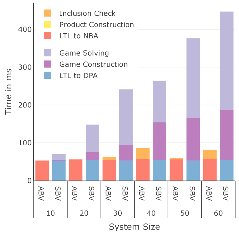
Figure 3: Comparison of ABV and SBV on instances of varying system size and fixed property size of 20. We generate 100 random instances for each size and take the average over the fastest $L$ instances, where $L$ is the minimum number of instances solved within a 5s timeout by both methods.

SBV is known to be incomplete [18, 8]. However, due to the previous lack of complete tools for verifying $\forall^{*}\exists^{*}$ properties, a detailed study into how effective SBV is in practice was impossible on a larger scale (i.e., beyond hand-crafted examples). With AutoHyper, we can, for the first time, rigorously evaluate SBV. We use the SBV implementation from [8], which synthesizes a strategy for the $\exists$-player by translating the formula to a deterministic parity automaton (DPA) [34] and phrases the synthesizes as a parity game.

We have generated random transition systems and properties of varying sizes and computed a ground truth using AutoHyper. We then performed SBV (recall that SBV can never show that a property does not hold and might fail to establish that it does). We find that for our generated instances, the property holds in 61.1% of the cases, and SBV can verify the property in 60.4% of the cases. Successful verification with SBV is thus possible in many cases, even without the addition of expensive mechanisms such as prophecies [8]. On the other hand, our results show that random generation produces instances (albeit not many) on which SBV fails (so far, examples where SBV fails required careful construction by hand). Reverting to SBV as the default verification strategy is thus not possible, further strengthening the case for complete model checking tools (of which AutoHyper is the first).

8.2 Efficiency of Strategy-based Verification

After having analyzed the effectiveness of SBV (i.e., how many instances can be verified), we turn our attention to the efficiency of SBV. In theory, (automata-based) model checking of $\forall^{*}\exists^{*}$ HyperLTL – as implemented in AutoHyper – is EXPSPACE-complete in the specification and PSPACE-complete in the size of the system [14, 35]. Conversely, SBV is $2$-EXPTIME-complete in the size of the specification but only PTIME in the size of the system [18]. Consequently, one would expect that ABV fares better on larger specifications and SBV fares better on larger systems (the more important measure in practice).

However, in this section, we show that this does not translate into practice (at least using the current implementation of SBV [8]). We compare the running time of AutoHyper (ABV) (using spot’s inclusion checker) and SBV. We break the running time into the three main steps for each method. For ABV, this is the LTL-to-NBA translation, the construction of the product automaton, and the inclusion check. For SBV, it is the LTL-to-DPA translation, the construction of the game, and the game-solving.

We depict the average cost for varying system sizes in Figure 3. We observe that SBV performs worse than ABV and, more importantly, scales poorly in the size of the system. This is contrary to the theoretical analysis of ABV and SBV. As the detailed breakdown of the running time suggests, the poor performance is due to the costly construction of the game and the time taken to solve the game. An almost identical picture emerges if we compare ABV in SBV relative to the property size (we give a plot in Appendix 0.E.1). While, in this case, the results match the theory (i.e., SBV scales worse in the size of the specification), we find that the bottleneck for SBV is not the LTL-to-DPA translation (which, in theory, is exponentially more expensive than the LTL-to-NBA translation used in ABV), but, again the construction and solving of the parity game.

We remark that the SBV engine we used [8] is not optimized and always constructs the full (reachable) game graph. The poor performance of SBV can be attributed to the fact that the size of the game does, in the worst case, scale quadratically in the size of the system (when considering $\forall^{1}\exists^{1}$ properties). This is amplified in dense systems (i.e., systems with many transitions), as, with increasing transition density, the size of the parity games approaches its worst-case size (see Appendix 0.E). In contrast, the heavily optimized inclusion checker (in this case spot) seems to be able to check inclusion in almost constant time (despite being exponential in theory). This efficiency of mature language inclusion checkers is what enables AutoHyper to achieve remarkable performance that often exceeds that of symbolic methods such as BMC (cf. Section 7) and further strengthens the practical impact of Proposition 1.

9 Conclusion

In this paper, we have presented AutoHyper, the first complete model checker for HyperLTL with an arbitrary quantifier prefix. We have demonstrated that AutoHyper can check many interesting properties involving quantifier alternations and often outperforms symbolic methods such as BMC, sometimes by orders of magnitude. We believe the biggest advantage of AutoHyper to be its push-button functionality combined with its completeness: As a user, one does not need to worry whether AutoHyper is applicable to a particular property (different from, e.g., SBV or BMC) and does not need to provide hints (e.g., in the form of explicit strategies in SBV).

Apart from evaluating AutoHyper’s performance on a range of benchmarks, we have used AutoHyper to (1) compare various backend language inclusion checkers, (2) explore practical verification beyond one quantifier alternation (which is not as infeasible as suggested by the theory), and (3) rigorously evaluate the effectiveness and efficiency of strategy-based verification in practice (which, different than suggested by a theoretical analysis, performs worse than automata-based methods).

9.0.1 Acknowledgments.

This work was partially supported by the DFG in project 389792660 (Center for Perspicuous Systems, TRR 248), and by by the ERC Grant HYPER (No. 101055412). R. Beutner carried out this work as a member of the Saarbrücken Graduate School of Computer Science.

Data Availability Statement

AutoHyper and all experiments are available at [4].

Appendix 0.A HyperLTL Model Checking and Language Inclusion

See 1

Proof

For the first direction we assume that $\mathcal{L}(\mathcal{A}^{n}_{\mathcal{T}})\subseteq\mathcal{L}(\mathcal{A}_{\varphi})$ and need to show that $\mathcal{T}\models\dot{\varphi}=\forall\pi_{1}.\ldots\forall\pi_{n}.\varphi$. So let $t_{1},\ldots,t_{n}\in\mathit{Traces}(\mathcal{T})$ be arbitrary. By definition we have $\mathit{zip}(t_{1},\ldots,t_{n})\in\mathcal{L}(\mathcal{A}^{n}_{\mathcal{T}})$ and so by assumption $\mathit{zip}(t_{1},\ldots,t_{n})\in\mathcal{L}(\mathcal{A}_{\varphi})$. By $\mathcal{T}$-equivalence of $\mathcal{A}_{\varphi}$ this implies $[\pi_{1}\mapsto t_{1},\cdots,\pi_{n}\mapsto t_{n}]\models_{\mathit{Traces}(\mathcal{T})}\varphi$ as required.

For the reverse we assume that $\mathcal{T}\models\dot{\varphi}$ and need to show that $\mathcal{L}(\mathcal{A}^{n}_{\mathcal{T}})\subseteq\mathcal{L}(\mathcal{A}_{\varphi})$. Let $t\in\mathcal{L}(\mathcal{A}^{n}_{\mathcal{T}})$ be arbitrary. By definition of $\mathcal{A}_{\mathcal{T}}$ and $\mathit{zip}$ we have $t=\mathit{zip}(t_{1},\ldots,t_{n})$ for some $t_{1},\ldots,t_{n}\in\mathit{Traces}(\mathcal{T})$. As $\mathcal{T}\models\dot{\varphi}=\forall\pi_{1}.\ldots\forall\pi_{n}.\varphi$ we have $[\pi_{1}\mapsto t_{1},\cdots,\pi_{n}\mapsto t_{n}]\models_{\mathit{Traces}(\mathcal{T})}\varphi$. By $\mathcal{T}$-equivalence this implies $t=\mathit{zip}(t_{1},\ldots,t_{n})\in\mathcal{L}(\mathcal{A}_{\varphi})$ as required. ∎

Appendix 0.B Overview of Verification Methods

In recent years, many different methods to verify HyperLTL properties have been developed. In the following, we summarize the existing approaches (possibly repeating information from the main body) and briefly discuss their relative strengths and weaknesses in Section 0.B.

Alternation-free HyperLTL and Manual Strengthening.

HyperLTL properties without quantifier alternations can be reduced to checking a trace property on the self-composition of the system [3] and thus have the same model checking complexity as LTL (NL-complete in the size of the system and PSPACE-complete in the size of the formula). This verification approach for HyperLTL has been implemented in McHyper [28]. By using ABC [11] as the backend solver, McHyper is applicable to circuits with thousands of latches. This is well beyond the reach of explicit-state model checking approaches.

While McHyper supports only alternation-free formulas, Finkbeiner et al. [28] and D’Argenio et al. [21] use it to verify properties involving quantifier alteration by manually strengthening them into alternation-free formulas. For example, a $\forall\exists$ property can be strengthened by replacing the existential quantification with a universal one, resulting in a $\forall\forall$ property. The soundness of this strengthening must be argued manually and cannot be checked automatically. Moreover, such strengthening is specific to a property and – more importantly – also to the model; the method is thus not applicable to general HyperLTL MC.

Strategy-based Verification.

Coenen et al. [18] verify $\forall^{*}\exists^{*}$ properties by instating the existential quantification with an explicit strategy. This method – which we refer to as strategy-based verification (SBV) – comes in two flavors: either the strategy is provided by the user or the strategy is synthesized. In the former case, model checking directly reduces to checking an alternation-free formula (which is cheap). In fact, model checking with a given strategy is as expensive as checking alternation-free HyperLTL (NL-complete in the system) and can be performed on systems of considerable size. On the other hand, supplying an explicit strategy requires deep insight into the system. Different from BMC (as in HyperQube) or explict-state MC (as in AutoHyper), verification with a given strategy is thus no push-button technique which is why we did not evaluate against it. In the latter case, the method works fully automatically but requires a more expensive strategy synthesis. SBV with automated strategy synthesis is, in theory, more efficient than ABV (in the size of the system): In theory, (automata-based) model checking of $\forall^{*}\exists^{*}$ HyperLTL – as implemented in AutoHyper – is EXPSPACE-complete in the specification and PSPACE-complete in the size of the system [14, 35]. Conversely, SBV is $2$-EXPTIME-complete in the size of the specification but PTIME in the size of the system [18]. SBV is, however, incomplete as the strategy resolving existentially quantified traces only observes finite prefixes of the universally quantified traces (for examples see, e.g., [8]). While prophecies have recently been proposed as a countermeasure to ensure completeness [8], no efficient method for the synthesis of prophecies exists. Current synthesis approaches for prophecies are limited to systems with $\leq 20$ states [8].

	Sound	AA	Symbolic	PB	NL	Complete
Manual Strengthening [28, 21]
SBV[Explicit Strategy] [18]
SBV[Strategy Synthesis] [8, 9]
BMC [30]
Explicit ABV [This work]

Figure 4: We list existing verification approaches for HyperLTL together with their advantages and disadvantage. means that the “property” holds, that it does not, and indicates that no clear answer is possible. We abbreviate: AA = Arbitrary alternation; Symbolic = Support for symbolic systems; PB = Push-button technique; NL=very efficient (NL) model checking in the size of the system.

Bounded Model Checking.

Hsu et al. [30] proposed a bounded model checking (BMC) procedure for HyperLTL. Similar to BMC for trace properties (see e.g., [10]) the formula is unfolded up to a fixed depth and pending obligations beyond that depth are either treated pessimistically (allowing to witness the satisfaction of a formula) or optimistically (allowing to witness the violation of a formula). While BMC for trace properties reduces to a SAT-solving, BMC for hyperproperties naturally reduces to a QBF-solving. The BMC approach is implemented in HyperQube. As usual for bounded methods, BMC for HyperLTL is incomplete. For example, it can never show that a system satisfies a hyperproperty of the form $\mathbb{Q}_{1}\pi_{1}.\ldots\mathbb{Q}_{n}\pi_{n}.\operatorname{\leavevmode\hbox to6.97pt{\vbox to6.97pt{\text{[drawing]}}}}\psi$ such as GNI. In case the system terminates after a fixed number of steps (i.e., reaches a state whose only outgoing transition is to itself), pending obligations in that state can be evaluated precisely (as the entire future execution is fixed). Hsu et al. [30] use this observation in their so-called halting semantics (which comes in both an optimistic and a pessimistic flavor). While this improves the accuracy of BMC (for example, the halting semantics can verify GNI if all executions of a system terminates after $k$ steps and the unrolling bound is some $k^{\prime}\geq k$), most reactive systems are inherently non-terminating. All of the examples considered in Table 1 are non-terminating (as is usual for rwsctive programs), so the halting semantics offers no advantage – GNI cannot be verified in any of those systems.

Strengths and Weaknesses

An informal but illustrative overview of the relative strengths and weaknesses of each method is depicted in Figure 4. As expected, all methods are sound (although for the manual strengthening the soundness argument cannot be checked automatically). Different from BMC and ABV, SBV is limited to $\forall^{*}\exists^{*}$ formulas and cannot cope with arbitrary quantifier alternations. The biggest disadvantage of explicit-state MC is that it is not applicable to symbolic systems (such as circuits) and requires a prior conversion to an explicit system. Nevertheless, in this paper, we show that – at least for the existing set of benchmarks – explicit MC performs on-par, or even outperforms, many symbolic methods by internally converting to an explicit-state representation. SBV with strategy synthesis is, in theory, applicable to symbolic systems by solving a symbolic parity game, but this is currently not supported by any tool (hence the ). Manual strengthening and SBV with a given strategy are both very cheap (i.e., NL in the size of the system) but require significant manual effort that often requires domain knowledge. In contrast, SBV with strategy synthesis, BMC, and ABV and theoretically more expensive but “push-button techniques”, i.e., they require no manual input by the user. Performance-wise BMC occupies a useful middle ground: while not as efficient as alternation-free methods, it reduces to the QBF problem that can, in theory, be solved faster than automaton-theoretic problems encountered in explicit-state model checking. As we show in Section 7, this does not translate to practice and ABV can often compete with the performance of BMC. Finally, the biggest motivation for the study of ABV (in the form of AutoHyper) is its completeness; AutoHyper is the first tool that can verify arbitrary HyperLTL properties in a sound-and-complete way.

Appendix 0.C HyperLTL MC as Language Inclusion Benchmarks

When comparing BAIT and RABIT in detail, the instances arising during HyperLTL MC seem to heavily favor RABIT (see Figure 1). This is in contrast to the observations made in [24], who found that BAIT outperforms RABIT on a majority of existing language inclusion benchmarks. Verification of $\forall^{*}\exists^{*}$ HyperLTL is, therefore, a natural candidate to extend the existing set of automaton inclusion benchmarks (an area where benchmarks are still sparse, see, e.g., [24]). The resulting benchmarks seem to cover instances different from those found in existing benchmark sets (as indicated by the drastically different performance of BAIT and RABIT on both benchmark families).

Appendix 0.D Plan Synthesis as HyperLTL Model Checking

We note that path planning problem as studied by Wang et al. [38], involve the synthesis of a plan. If we wish to synthesize the shortest path, we can phrase the problem as a formula $\varphi=\exists\pi\mathpunct{.}\forall\pi^{\prime}.\psi$ wher $\psi$ states that $\pi$ encodes a path that reaches the goal and all other paths $\pi^{\prime}$ take at least as long as $\pi$. A concrete witness trace for $\pi$ is then an optimal solution to the planning problem. When checking $\varphi$ by reducing an SMT query (as done by Wang et al. [38]) or to a QBF problem (as done by Hsu et al. [30]) we can easily extract a concrete solution from a satisfying model of the encoding (which is either $\exists^{*}\forall^{*}$ SMT or an $\exists^{*}\forall^{*}$ QBF formula). Synthesizing a concrete path using the automaton-based approach implemented in AutoHyper is less straightforward. However, we argue that we can actually use the approach to synthesize a concrete solution, provided the used language inclusion checker provides counterexamples (which is the case for most solver such as RABIT, BAIT, and FORKLIFT).

In AutoHyper, we check the negated $\neg\varphi=\forall\pi\mathpunct{.}\exists\pi^{\prime}.\neg\psi$ formula as this allows us to make use of language inclusion checkers. As the model satisfies $\varphi$ (all models that have a shortest path will satisfy $\varphi$), it violates $\neg\varphi$, so by Proposition 1, the language inclusion that is checked does not hold. A trace $t$ that witnesses this non-inclusion during the model checking of $\neg\varphi$ property is thus contained in the system but has no witness trace; Or phrased equivalently, $t$ is a witness for the existential quantification in $\varphi$. Language inclusion checkers that return counterexamples can thus be used for optimal path planning and (as shown in Table 3) outperform the QBF-based approach.

Appendix 0.E Details for Section 8

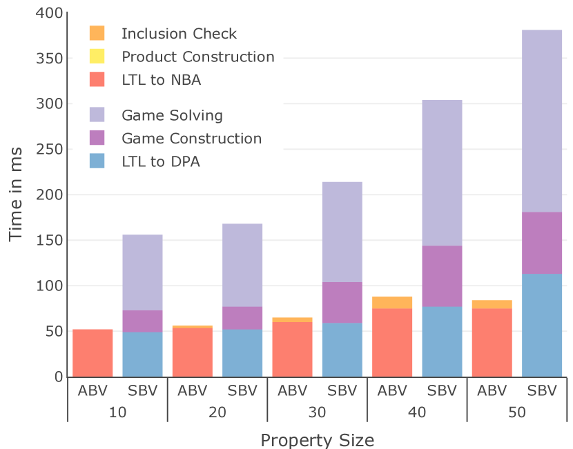
(a) Running times of ABV and SBV with varying property size. We fix the system size 30.

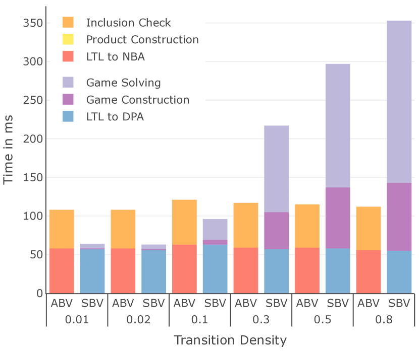
(b) Running times of ABV and SBV with varying transition density. We fix the system size to 30, and the property size to 20.

Figure 5: We compare ABV and SBV on instances with varying property size (in Figure 5(a)) and transition density (in Figure 5(b)). For each size we generate 100 random $\forall^{1}\exists^{1}$ properties. The timeout is set to 5s. We take the average over the fastest $L$ instances, where $L$ is the minimum of the instances solved within a 5s timeout by both ABV and SBV.

0.E.1 Efficiency of SBV – Impact of Specification Size

Similar to Figure 3, Figure 5(a) compares the running time of ABV and SBV in terms of the property size. While these results match the theory, i.e., SBV scales worse than ABV in the size of the specification, the detailed breakdown of the total running time shows that the decrease in performance is not for the reason suggested by theory. While the limiting factor should be a much more expensive LTL-to-DPA translation (which is exponentially more expensive than a LTL-to-NBA translation involved in ABV) the actual blowup stems from the construction and solving time of the parity game.

0.E.2 Efficiency of SBV – Impact of Transition Density

We perform a similar experiment as in Figures 3 and 5(a) but do no vary the size of the transition system but only its density. Figure 5(b) depicts the results. We observe that with increasing density, SBV scales very poorly. This confirms that the poor performance of SBV is due to the size of the game space, which, with increasing transition density, approaches quadratic size (in the size of the system). To see this, take a system with $n$ states where each state has a unique successor. The resulting parity game constructs the $2$-fold self-composition of the system, which has $\Theta(n)$ states. At the other extreme, if each state has a transition to all other states, the resulting game has size $\Theta(n^{2})$ as all pairs of states occur in the product.

References

- [1] Babiak, T., Blahoudek, F., Duret-Lutz, A., Klein, J., Kretínský, J., Müller, D., Parker, D., Strejcek, J.: The Hanoi omega-automata format. In: International Conference on Computer Aided Verification, CAV 2015. LNCS, vol. 9206. Springer (2015). https://doi.org/10.1007/978-3-319-21690-4_31
- [2] Baier, C., Katoen, J.P.: Principles of model checking. MIT press (2008)
- [3] Barthe, G., D’Argenio, P.R., Rezk, T.: Secure information flow by self-composition. Math. Struct. Comput. Sci. 21(6) (2011). https://doi.org/10.1017/S0960129511000193
- [4] Beutner, R.: AutoHyper: Explicit-state model checking for HyperLTL (2023). https://doi.org/10.5281/zenodo.7309986
- [5] Beutner, R., Carral, D., Finkbeiner, B., Hofmann, J., Krötzsch, M.: Deciding hyperproperties combined with functional specifications. In: Annual ACM/IEEE Symposium on Logic in Computer Science, LICS 2022. ACM (2022). https://doi.org/10.1145/3531130.3533369
- [6] Beutner, R., Finkbeiner, B.: A temporal logic for strategic hyperproperties. In: International Conference on Concurrency Theory, CONCUR 2021. LIPIcs, vol. 203. Schloss Dagstuhl (2021). https://doi.org/10.4230/LIPIcs.CONCUR.2021.24
- [7] Beutner, R., Finkbeiner, B.: HyperATL*: A logic for hyperproperties in multi-agent systems. CoRR abs/2203.07283 (2022). https://doi.org/10.48550/arXiv.2203.07283
- [8] Beutner, R., Finkbeiner, B.: Prophecy variables for hyperproperty verification. In: IEEE Computer Security Foundations Symposium, CSF 2022. IEEE (2022). https://doi.org/10.1109/CSF54842.2022.00030, https://arxiv.org/abs/2206.01797
- [9] Beutner, R., Finkbeiner, B.: Software verification of hyperproperties beyond k-safety. In: International Conference on Computer Aided Verification, CAV 2022. LNCS, vol. 13371. Springer (2022). https://doi.org/10.1007/978-3-031-13185-1_17
- [10] Biere, A., Cimatti, A., Clarke, E.M., Zhu, Y.: Symbolic model checking without BDDs. In: International Conference on Tools and Algorithms for Construction and Analysis of Systems, TACAS 1999. LNCS, vol. 1579. Springer (1999). https://doi.org/10.1007/3-540-49059-0_14
- [11] Brayton, R.K., Mishchenko, A.: ABC: an academic industrial-strength verification tool. In: International Conference on Computer Aided Verification, CAV 2010. LNCS, vol. 6174. Springer (2010). https://doi.org/10.1007/978-3-642-14295-6_5
- [12] Cimatti, A., Clarke, E.M., Giunchiglia, E., Giunchiglia, F., Pistore, M., Roveri, M., Sebastiani, R., Tacchella, A.: NuSMV 2: An opensource tool for symbolic model checking. In: International Conference on Computer Aided Verification, CAV 2002,Copenhagen. LNCS, vol. 2404. Springer (2002). https://doi.org/10.1007/3-540-45657-0_29
- [13] Clarke, E.M., Kroening, D., Ouaknine, J., Strichman, O.: Completeness and complexity of bounded model checking. In: International Conference on Verification, Model Checking, and Abstract Interpretation, VMCAI 2004. LNCS, vol. 2937. Springer (2004). https://doi.org/10.1007/978-3-540-24622-0_9
- [14] Clarkson, M.R., Finkbeiner, B., Koleini, M., Micinski, K.K., Rabe, M.N., Sánchez, C.: Temporal logics for hyperproperties. In: International Conference on Principles of Security and Trust, POST 2014. LNCS, vol. 8414. Springer (2014). https://doi.org/10.1007/978-3-642-54792-8_15
- [15] Clarkson, M.R., Schneider, F.B.: Hyperproperties. In: IEEE Computer Security Foundations Symposium, CSF 2008. IEEE (2008). https://doi.org/10.1109/CSF.2008.7
- [16] Clemente, L., Mayr, R.: Efficient reduction of nondeterministic automata with application to language inclusion testing. Log. Methods Comput. Sci. 15(1) (2019). https://doi.org/10.23638/LMCS-15(1:12)2019
- [17] Coenen, N., Finkbeiner, B., Frenkel, H., Hahn, C., Metzger, N., Siber, J.: Temporal causality in reactive systems. In: International Symposium on Automated Technology for Verification and Analysis, ATVA 2022. LNCS, vol. 13505. Springer (2022). https://doi.org/10.1007/978-3-031-19992-9_13
- [18] Coenen, N., Finkbeiner, B., Sánchez, C., Tentrup, L.: Verifying hyperliveness. In: International Conference on Computer Aided Verification, CAV 2019. LNCS, vol. 11561. Springer (2019). https://doi.org/10.1007/978-3-030-25540-4_7
- [19] Copty, F., Fix, L., Fraer, R., Giunchiglia, E., Kamhi, G., Tacchella, A., Vardi, M.Y.: Benefits of bounded model checking at an industrial setting. In: International Conference on Computer Aided Verification, CAV 2001. LNCS, vol. 2102. Springer (2001). https://doi.org/10.1007/3-540-44585-4_43
- [20] Courcoubetis, C., Vardi, M.Y., Wolper, P., Yannakakis, M.: Memory-efficient algorithms for the verification of temporal properties. Formal Methods Syst. Des. 1(2/3) (1992). https://doi.org/10.1007/BF00121128
- [21] D’Argenio, P.R., Barthe, G., Biewer, S., Finkbeiner, B., Hermanns, H.: Is your software on dope? - formal analysis of surreptitiously "enhanced" programs. In: European Symposium on Programming, ESOP 2017. LNCS, vol. 10201. Springer (2017). https://doi.org/10.1007/978-3-662-54434-1_4
- [22] Doherty, S., Detlefs, D., Groves, L., Flood, C.H., Luchangco, V., Martin, P.A., Moir, M., Shavit, N., Jr., G.L.S.: DCAS is not a silver bullet for nonblocking algorithm design. In: Annual ACM Symposium on Parallelism in Algorithms and Architectures, SPAA 2004. ACM (2004). https://doi.org/10.1145/1007912.1007945
- [23] Doveri, K., Ganty, P., Mazzocchi, N.: FORQ-based language inclusion formal testing. In: International Conference on Computer Aided Verification, CAV 2022. LNCS, vol. 13372. Springer (2022). https://doi.org/10.1007/978-3-031-13188-2_6
- [24] Doveri, K., Ganty, P., Parolini, F., Ranzato, F.: Inclusion testing of Büchi automata based on well-quasiorders. In: International Conference on Concurrency Theory, CONCUR 2021. LIPIcs, vol. 203. Schloss Dagstuhl (2021). https://doi.org/10.4230/LIPIcs.CONCUR.2021.3
- [25] Duret-Lutz, A., Renault, E., Colange, M., Renkin, F., Aisse, A.G., Schlehuber-Caissier, P., Medioni, T., Martin, A., Dubois, J., Gillard, C., Lauko, H.: From Spot 2.0 to Spot 2.10: What’s new? In: International Conference on Computer Aided Verification, CAV 2022. LNCS, vol. 13372. Springer (2022). https://doi.org/10.1007/978-3-031-13188-2_9
- [26] Fellner, A., Befrouei, M.T., Weissenbacher, G.: Mutation testing with hyperproperties. Softw. Syst. Model. 20(2) (2021). https://doi.org/10.1007/s10270-020-00850-1
- [27] Fienberg, S.E.: A brief history of statistical models for network analysis and open challenges. Journal of Computational and Graphical Statistics 21(4) (2012)
- [28] Finkbeiner, B., Rabe, M.N., Sánchez, C.: Algorithms for model checking HyperLTL and HyperCTL*. In: International Conference on Computer Aided Verification, CAV 2015. LNCS, vol. 9206. Springer (2015). https://doi.org/10.1007/978-3-319-21690-4_3
- [29] Herlihy, M., Wing, J.M.: Linearizability: A correctness condition for concurrent objects. ACM Trans. Program. Lang. Syst. 12(3) (1990). https://doi.org/10.1145/78969.78972
- [30] Hsu, T., Sánchez, C., Bonakdarpour, B.: Bounded model checking for hyperproperties. In: International Conference on Tools and Algorithms for the Construction and Analysis of Systems, TACAS 2021. LNCS, vol. 12651. Springer (2021). https://doi.org/10.1007/978-3-030-72016-2_6
- [31] Jamroga, W., Mauw, S., Melissen, M.: Fairness in non-repudiation protocols. In: International Workshop on Security and Trust Management, STM 2011. LNCS, vol. 7170. Springer (2011). https://doi.org/10.1007/978-3-642-29963-6_10
- [32] Lamport, L.: A new solution of dijkstra’s concurrent programming problem. Commun. ACM 17(8) (1974). https://doi.org/10.1145/361082.361093
- [33] McCullough, D.: Noninterference and the composability of security properties. In: IEEE Symposium on Security and Privacy, SP 1988. IEEE (1988). https://doi.org/10.1109/SECPRI.1988.8110
- [34] Piterman, N.: From nondeterministic Büchi and Streett automata to deterministic parity automata. Log. Methods Comput. Sci. 3(3) (2007). https://doi.org/10.2168/LMCS-3(3:5)2007
- [35] Rabe, M.N.: A temporal logic approach to Information-flow control. Ph.D. thesis, Saarland University (2016)
- [36] Smith, G., Volpano, D.M.: Secure information flow in a multi-threaded imperative language. In: ACM SIGPLAN-SIGACT Symposium on Principles of Programming Languages, POPL 1998. ACM (1998). https://doi.org/10.1145/268946.268975
- [37] Tsai, M., Tsay, Y., Hwang, Y.: GOAL for games, omega-automata, and logics. In: International Conference on Computer Aided Verification, CAV 2013. LNCS, vol. 8044. Springer (2013). https://doi.org/10.1007/978-3-642-39799-8_62
- [38] Wang, Y., Nalluri, S., Pajic, M.: Hyperproperties for robotics: Planning via HyperLTL. In: IEEE International Conference on Robotics and Automation, ICRA 2020. IEEE (2020). https://doi.org/10.1109/ICRA40945.2020.9196874