Time-consistency in the mean-variance problem: A new perspective

Nicole Bäuerle Department of Mathematics, Karlsruhe Institute of Technology (KIT), Karlsruhe, Germany nicole.baeuerle@kit.edu  and  Anna Jaśkiewicz Faculty of Pure and Applied Mathematics, Wrocław University of Science and Technology, Wrocław, Poland anna.jaskiewicz@pwr.edu.pl
Abstract.

We investigate discrete-time mean-variance portfolio selection problems viewed as a Markov decision process. We transform the problems into a new model with deterministic transition function for which the Bellman optimality equation holds. In this way, we can solve the problem recursively and obtain a time-consistent solution, that is an optimal solution that meets the Bellman optimality principle. We apply our technique for solving explicitly a more general framework.

Key words:

Bellman optimality principle, time-consistency, mean-variance portfolio selection, linear-quadratic optimal control

1. Introduction

The Bellman optimality principle is one of the key results in optimal control theory. It asserts that the optimization of dynamic processes with finite time horizon is equivalent to the solution of a recursive equation also known as a dynamic program, dynamic programming problem or Bellman optimality equation. The part of operations research concerned with Markov decision processes (MDPs) is sometimes called dynamic programming.

From the dynamic programming principle, it follows that an optimal policy established for the initial points (time and state) is also optimal along the optimal trajectory. This property is referred to as the time-consistency of the optimal policy, see Subsec. 1.2 in [6]. However, in reality, the Bellman principle often fails. It occurs when a dynamic optimization problem is not time additively separable, or simply, non-separable. Mathematically, it means that the optimal value cannot be separated into the sum of the present payoff and the optimal value term derived from tomorrow. The mean-variance optimization criterion belongs to this class of non-separable models. The nonlinear term of the (conditional) variance in the cost functional causes the time-inconsistency, since it spoils the iterated-expectations property. For Markov decision models, this problem was analyzed in different settings, for instance, in [12, 20] and [15] for discrete-time processes and in [13] for continuous-time processes. In [12], the method, based on a penalty for the variability in the stream of rewards, allows to obtain a solution via linear programming, whereas in [20] Pareto optima in the sense of high mean and low variance of the stationary probability distribution are considered. The objective of [15], on the other hand, is to compare different policy classes and discusses computational complexity.

A prominent problem in the financial economics for this optimization criterion is the mean-variance portfolio selection model. There are two main approaches that provide a solution. In the first one, the investor fixes the initial point (time and state) and finds the optimal policy that minimizes his objective cost functional. In other words, the agent pre-commits to follow the derived strategy, although at future dates it is not longer optimal. The second solution is based on a game theoretic approach. Namely, the investor plays an intrapersonal game, whose outcome is a subgame perfect equilibrium. To apply this technique, the objective function is decomposed into the investor’s expected future objective plus an additional term that controls his deviations. This method leads to a certain recursive formula, which produces a suboptimal solution. Therefore, the obtained strategy is sometimes called dynamically optimal [2] or time-consistent dynamically optimal [21] or time-consistent [10]. However, in this paper we follow the definition of the time-consistency given in [6] (see also Definition 2.1).

The literature contains a number of examples of the outlined approaches. For obvious reasons, we describe here only some positions. The paper of Li and Ng [14] is the first work on a dynamic mean-variance portfolio model in discrete-time. The optimal policy is obtained by an embedding method that transforms the original problem into a standard linear-quadratic (LQ) model. This leads to time-inconsistency of an investor’s strategy. Alternatively, as noted by Yoshida [22], the multi-period mean-variance portfolio selection problem can be solved explicitly under the so-called deterministic mean-variance trade-off condition. The latter approach that generates a subgame perfect equilibrium was applied in [6] for discrete-time models and in [2, 7] for continuous-time models. All these three papers handle a Markovian setting, whereas the non-Markovian framework was studied in [10]. Finally, there is also a possibility to optimize the conditional mean-variance criterion myopically in each step separately over the payoffs in the next period, see [8].

Apart from the aforementioned methodologies, Cui et al. [9] suggests mean-field techniques to deal with time-inconsistency in this model. The idea is to include the expected values of the state process into the underlying dynamic system and the objective functional. In such a way, the problem becomes separable but it is constrained. Their approach was generalized in [1] for discrete-time linear systems with multiplicative noise. As an application, the multi-period optimal control policy for a general mean-variance problem was derived. An alternative approach, based on mean-field theory and establishing the pre-commitment optimal solution in the continuous time mean-variance portfolio selection problem was provided in [5]. In particular, it was proved that the optimal policy satisfies a Hamilton-Jacobi-Bellman equation that also involves the probability distribution of the corresponding optimal wealth process.

In this paper, we start our analysis from the discrete-time mean-variance portfolio selection problem modelled by an MDP. Although the problem is time-inconsistent, we show that this is not true if more information is included. More precisely, our idea relies on a replacement of the original state space (the levels of the wealth) by the set of probability measures on it. This trick, in turn, allows us to transform the original MDP into a purely deterministic model, for which we are able to write a standard Bellman equation. We refer to this new model as a population version MDP. Thus, we provide for the first time a backward induction algorithm that generates the time-consistent policy. Furthermore, we show that if the initial distribution is the Dirac delta concentrated at some point $x_{0}$, then the investor’s time-consistent strategy (i.e., the strategy that is optimal and satisfies the Bellman optimality principle) from the population version MDP coincides with the pre-commitment optimal strategy given in [14] or [4]. We also discuss and compare the optimal policy with a suboptimal solution based on game theoretic tools.

Next we apply our approach to more general time-inconsistent problems outlined in Subsec. 1.6 in [6]. We deal with the case, where the cost functions in the objective functional are independent of the initial points (time and state). Within a population version MDP framework, the Bellman optimality principle works and a time-consistent policy exists. As an application, we solve an LQ regulator problem and compare our solution with the equilibrium strategy from [6]. It is worthy to mention that LQ control models were also studied in the mean-field setting, see [11, 18, 17] or [19]. However, as noted in [9], this direction requires new analytical tools and solution techniques. Therefore, within this view our method demonstrates a direct and simple way in dealing with time-inconsistent problems that improves the quality of the solutions.

The paper is organized as follows. In Sec. 2 we present the multi-period portfolio selection problem and describe three approaches. Sec. 3 generalizes our techniques to solve an MDP in the finite time-horizon, in which the cost functional contains a non-linear term. Our findings are applied to an LQ model in Sec. 4. A relationship to the mean-field framework and possible extensions are discussed in Sec. 5. Finally, we conclude in Sec. 6. The last part, Sec. 7, is devoted to solving one-step models from Sections 2 and 4.

2. Mean-variance problem

We start with the definition of a time-consistent solution taken from [6].

Definition 2.1.

Assume that we have an $N$-finite time horizon optimization problem $\mathcal{P}(0,x)$ starting at time point 00 with an initial state $x.$ Suppose that the optimal control is ${\bf u}=(u^{0,x}_{0},u^{0,x}_{1},\ldots,u^{0,x}_{N}).$ The optimal control is time-consistent, if it satisfies the Bellman optimality principle, i.e., it is also optimal on the time interval $\{n,\ldots,N\}$ for any $n\in\{1,\ldots,N-1\}.$

According to this definition, a time-consistent control must be optimal for the problem $\mathcal{P}(0,x)$ and, roughly speaking, ${\bf u}$ must be independent of the initial state. More formally, this means that the optimal control for $\mathcal{P}(n,y)$ is $(u^{n,y}_{n},\ldots,u^{n,y}_{N}),$ where $u^{n,y}_{k}=u^{0,x}_{k}$ for all time points $n\leq k\leq N$ and states $x,y.$

The mean-variance problem is often cited as a problem, where the optimal policy is not time-consistent. The reason for the time-inconsistency in this model is the conditional variance term. Although the tower property holds for the conditional expectation, it does not hold for the conditional variance term. The reader is referred to [2] or [10] for the specific formula for this expression and further discussion. This fact, however, implies that a Bellman equation is not the standard Bellman equation anymore, because the value functions appearing on the left-hand side and right-hand side are not the same. In other words, the formulae for these functions are different. Hence, although we may use backward induction for deriving a solution, this solution need not be optimal, see Subsec. 2.3. The other approach is to find an optimal policy for the whole problem and not care at being optimal for any time interval $\{n,\ldots,N\},$ see Subsec. 2.2. It is known as a pre-commitment policy and it is not time-consistent. However, we show that this optimal solution can be seen as time-consistent and this is a question of information. More precisely, it becomes time-consistent, when we extend the state space. We will explain this in Subsec. 2.4. First we present the model and recalling the established approaches.

2.1. The model

Let $Y$ be a Borel set. We always equip it with its Borel $\sigma$-algebra $\mathcal{B}(Y).$ By $\Pr(Y)$ we denote the set of probability measures on $(Y,\mathcal{B}(Y)).$

Let us consider the following specific model which is taken from Sec. 4.6 in [4]. We have a financial market with one riskless bond. We assume that the riskless bond has interest rate $i_{n+1}$ during the period $[n,n+1)$, i.e.,

$$S_{n+1}^{0}=(1+i_{n+1})S^{0}_{n}\quad\mbox{for time points}\quad n=0,\ldots,N-1,\quad\mbox{where}\quad S_{0}^{0}\equiv 1.$$

In addition, we have $d$ risky assets with price processes

$$S_{n+1}^{k}=S_{n}^{k}\tilde{R}^{k}_{n+1},\quad k=1,\ldots,d,\quad n=0,\ldots,N-1$$

and $S_{0}^{k}\equiv 1$ for all $k,$ where $\tilde{R}^{k}_{n+1}$ are random variables on a joint probability space $(\Omega,\mathcal{F},\mathbb{P})$, which are assumed to be almost sure positive. In what follows, we use the notation $S_{n}^{\top}=(S_{n}^{1},\ldots,S_{n}^{d})$ and $\tilde{R}_{n}^{\top}=(\tilde{R}_{n}^{1},\ldots,\tilde{R}_{n}^{d})$. We assume that the random vectors $\tilde{R}_{1},\ldots\tilde{R}_{N}$ are independent. Further, let $R_{n}^{k}:=\frac{\tilde{R}_{n}^{k}}{1+i_{n}}-1$ and $R_{n}^{\top}=(R_{n}^{1},\ldots,R_{n}^{d})$ be the relative risk process. We further assume that $\mathbb{E}\|R_{n}\|<\infty,$ $\mathbb{E}R_{n}\neq 0$ and that the covariance matrix $\Sigma_{n}:=\big{(}Cov(R_{n}^{j},R_{n}^{k})\big{)}$ of these random vectors $R_{n}$ is positive definite for all $n$. We can invest into this financial market. Let $A_{n}^{\top}=(A^{1}_{n},\ldots,A_{n}^{d})\in\mathbb{R}^{d}.$ Here, $A_{n}^{k}$ is the amount of money invested into asset $k$ during time interval $[n,n+1)$. Thus, if $X_{n}$ denotes the wealth of the agent at time $n,$ then $X_{n}-A_{n}\cdot e,$ $e=(1,\ldots,1)^{\top}\in\mathbb{R}^{d}$ is the amount invested in the riskless bond, where $\cdot$ is the usual scalar product. Suppose that the initial wealth of the agent is $x_{0}\in\mathbb{R}.$ Then, the evolution of the wealth is given by the following difference equation

$$X_{n+1}=(1+i_{n+1})(X_{n}+A_{n}\cdot R_{n+1}).$$ (2.1)

The mean-variance model can be viewed as a non-stationary Markov decision process (MDP) with the following items:

  • $(E,\mathcal{B}(E))$ is the state space with $E:=\mathbb{R}$; here $x\in E$ denotes the wealth,

  • $(A,\mathcal{B}(A))$ is the action space with $A:=\mathbb{R}^{d};$ here $a\in A$ is the amount of money invested in the risky assets,

  • $\mathcal{R}:=[-1,\infty)^{d}$ is the space of values for the relative risk, i.e., $r\in\mathcal{R}$ denotes the relative risk,

  • $T_{n}(x,a,r)=(1+i_{n+1})(x+a\cdot r)$ is the transition function at time $n$, see (2.1), where $x\in E,$ $a\in A$ and $r\in\mathcal{R};$ the transition probability is given by

    $$Q_{n}(B|x,a)=\mathbb{P}\big{(}T_{n}(x,a,R_{n+1})\in B\big{)},\quad\mbox{where }B\in\mathcal{B}(E).$$

In what follows, let $\Pi$ be the set of all deterministic policies $\pi=(\pi_{0},\ldots,\pi_{N-1}).$ In other words, each $\pi_{n},$ $n=0,\ldots,N-1,$ is a measurable mapping defined on the history space of the process up to the $n$-th state with values in $A$. Moreover, let

$$F:=\{\phi:E\to A\ |\ \phi\mbox{ is measurable}\}.$$

Hence, $F$ is the set of decision rules that take into account only the current wealth of the agent. The sequence $(\phi_{0},\ldots,\phi_{N-1}),$ where $\phi_{k}\in F,$ $k=0,\ldots,N-1,$ determines a Markovian investment strategy to the agent.

Let $(\widetilde{\Omega},\widetilde{\mathcal{F}})$ be a measurable space with $\widetilde{\mathcal{F}}=\mathcal{B}(E)\otimes\cdots\otimes\mathcal{B}(E)$ ($N+1$ times). Then, for a fixed policy $\pi=(\pi_{0},\ldots,\pi_{N-1})\in\Pi$ and an initial state $x_{0}\in E$, a probability measure $\mathbb{P}^{\pi}_{x_{0}}$ is uniquely defined on $(\widetilde{\Omega},\widetilde{\mathcal{F}})$ according to the Ionescu-Tulcea theorem (see Appendix B in [4]). By $\mathbb{E}^{\pi}_{x_{0}}$ we denote the expectation operator with respect to the measure $\mathbb{P}^{\pi}_{x_{0}}.$

The mean-variance problem is given as a Lagrange problem by

$$P(\lambda)\left\{\begin{array}[]{l}Var_{x_{0}}^{\pi}[X_{N}]-2\lambda\mathbb{E}_{x_{0}}^{\pi}[X_{N}]\to\inf\\ \pi\in\Pi\end{array}\right.$$

where $\pi=(\pi_{0},\ldots,\pi_{N-1})\in\Pi$. Though not being separable, the problem can be solved with techniques from the theory of MDPs. Before we state and compare different solutions, let us define

$\displaystyle C_{n}:=\mathbb{E}[R_{n}R_{n}^{\top}],$ $\displaystyle\ell_{n}:=(\mathbb{E}[R_{n}])^{\top}C_{n}^{-1}\mathbb{E}[R_{n}]$
$\displaystyle d_{N}:=1,$ $\displaystyle d_{n}:=d_{n+1}(1-\ell_{n+1}),\quad n=0,\ldots,N-1.$ (2.2)

The matrix $C_{n}$ is positive definite and thus regular. It can also be shown that $\ell_{n},d_{n}\in(0,1)$ (see Lemma 4.6.4 in [4]).

2.2. Solution 1: Via auxiliary LQ-problems

Problem $P(\lambda)$ can be solved with the help of an auxiliary problem

$$QP(b)\left\{\begin{array}[]{l}\mathbb{E}_{x_{0}}^{\pi}[(X_{N}-b)^{2}]\to\inf\\ \pi\in F^{N}\end{array}\right.$$

which is a standard LQ-problem. In $QP(b)$ it is clear that we can replace $\Pi$ by $F^{N},$ since the optimal value will be attained under a Markovian investment strategy and $QP(b)$ can be solved by backward induction. The optimal policy for $QP(b)$ is for $n=0,1,\ldots,N-1$ and $x\in\mathbb{R}$ given by

$$\phi_{n}^{b}(x)=\Big{(}\frac{bS^{0}_{n}}{S^{0}_{N}}-x\Big{)}C_{n+1}^{-1}\mathbb{E}R_{n+1}.$$ (2.3)

This was shown in Theorem 4.6.5(b) in [4]. Further, we know that if $\pi^{b}=(\phi^{b}_{0},\ldots,\phi^{b}_{N-1})$ is optimal for $P(\lambda)$, then $\pi^{b}$ will also be optimal for $QP(b)$ with $b=\mathbb{E}_{x_{0}}^{\pi^{*}}[X_{N}]+\lambda$ (see Lemma 4.6.3 in [4]). Under $\pi^{b}$ the expected wealth is equal to

$\displaystyle\mathbb{E}_{x_{0}}^{\pi^{b}}[X_{N}]$ $\displaystyle=\mathbb{E}_{x_{0}}^{\pi^{b}}[(1+i_{N})(X_{N-1}+\phi_{N-1}^{b}(X_{N-1})\cdot R_{N})]$
$\displaystyle=\mathbb{E}_{x_{0}}^{\pi^{b}}\Big{[}(1+i_{N})\Big{(}X_{N-1}(1-R_{N}^{\top}C^{-1}_{N}\mathbb{E}R_{N})+\frac{bS^{0}_{N-1}}{S^{0}_{N}}R_{N}^{\top}C^{-1}_{N}\mathbb{E}R_{N}\Big{)}\Big{]}$
$\displaystyle=(1+i_{N})\Big{(}\mathbb{E}_{x_{0}}^{\pi^{b}}[X_{N-1}](1-\ell_{N})+\frac{bS^{0}_{N-1}}{S_{N}^{0}}\ell_{N}\Big{)}$
$\displaystyle=(1+i_{N})d_{N-1}\mathbb{E}_{x_{0}}^{\pi^{b}}[X_{N-1}]+b\ell_{N}$
$\displaystyle=(1+i_{N})d_{N-1}(1+i_{N-1})\Big{(}\mathbb{E}_{x_{0}}^{\pi^{b}}[X_{N-2}](1-\ell_{N-1})+\frac{bS^{0}_{N-2}}{S_{N}^{0}}\ell_{N-1}\Big{)}+b\ell_{N}$
$\displaystyle=(1+i_{N})(1+i_{N-1})d_{N-2}\mathbb{E}_{x_{0}}^{\pi^{b}}[X_{N-2}]+b\ell_{N-1}d_{N-1}+b\ell_{N}=\ldots$
$\displaystyle=\prod_{k=1}^{N}(1+i_{k})d_{0}x_{0}+b\sum_{k=1}^{N}\ell_{k}d_{k}=S^{0}_{N}d_{0}x_{0}+b\sum_{k=1}^{N}\ell_{k}d_{k}$
$\displaystyle=S^{0}_{N}d_{0}x_{0}+b(1-d_{0}).$ (2.4)

The last equality is due to the definition of $d_{n}$. Since $\ell_{k}d_{k}=d_{k}-d_{k-1}$ we obtain

$\displaystyle\sum_{k=1}^{N}\ell_{k}d_{k}$ $\displaystyle=$ $\displaystyle\sum_{k=1}^{N}(d_{k}-d_{k-1})=(d_{N}-d_{0})=1-d_{0}.$

Thus, when we set $b=\mathbb{E}_{x_{0}}^{\pi^{b}}[X_{N}]+\lambda,$ we obtain

$$b=S_{N}^{0}x_{0}+\frac{\lambda}{d_{0}}.$$ (2.5)

Plugging (2.5) into (2.3), we have partly proved the following:

Proposition 2.2.

An optimal policy $\pi^{o}=(\phi^{o}_{1},\ldots,\phi^{o}_{N-1})$ for $P(\lambda)$ is given by

$$\phi_{n}^{o}(x)=\Big{(}\Big{(}x_{0}+\frac{\lambda}{S_{N}^{0}d_{0}}\Big{)}S^{0}_{n}-x\Big{)}C_{n+1}^{-1}\mathbb{E}R_{n+1},\quad x\in E,$$

for $n=0,1,\ldots,N-1,$ and the value for $P(\lambda)$ is

$$V^{o}(x_{0}):=\lambda^{2}\Big{(}1-\frac{1}{d_{0}}\Big{)}-2\lambda x_{0}S_{N}^{0}.$$
Proof.

It remains to show the optimal value for $P(\lambda).$ From Theorem 4.5.6(c) in [4], we get under $\pi^{b}$ from (2.3) (see also the previous computation in (2.2)):

$\displaystyle\mathbb{E}_{x_{0}}^{\pi^{b}}[X_{N}]$ $\displaystyle=$ $\displaystyle x_{0}S_{N}^{0}d_{0}+b(1-d_{0}),$
$\displaystyle\mathbb{E}_{x_{0}}^{\pi^{b}}[X_{N}^{2}]$ $\displaystyle=$ $\displaystyle(x_{0}S_{N}^{0})^{2}d_{0}+b^{2}(1-d_{0}).$

Plugging (2.5) into above expressions, we easily get the conclusion. ∎

This policy is considered to be time-inconsistent, because the initial wealth $x_{0}$ enters the formula. Such a type of policy (depending on the current and initial states) is in MDP theory called a semi-Markov policy. In the economic and financial literature, it is sometimes known as a pre-commitment strategy. In other words, the agent cares only at being time consistent at the initial point $x_{0}$ and does not care of being time-consistent at future time points $n=1,\ldots,N-1.$ More precisely, if the wealth at time $n=1$ is $x_{1}\neq x_{0}$, then the previously computed restriction $(\phi^{o}_{1},\ldots,\phi^{o}_{N-1})$ is not optimal for the remaining time horizon.

Remark 2.3.

An alternative approach is to write $P(\lambda)$ as

$$P(\lambda)\left\{\begin{array}[]{l}\min_{b\in\mathbb{R}}\mathbb{E}_{x_{0}}^{\pi}\Big{[}(X_{N}-b)^{2}\Big{]}-2\lambda\mathbb{E}_{x_{0}}^{\pi}[X_{N}]\to\inf\\ \pi\in\Pi\end{array}\right.$$

using the fact that $Var(X)=\min_{b\in\mathbb{R}}\mathbb{E}[(X-b)^{2}]$. Since we can interchange the infima, we can first solve

$$\inf_{\pi\in\Pi}\mathbb{E}_{x_{0}}^{\pi}\Big{[}(X_{N}-b)^{2}\Big{]}-2\lambda\mathbb{E}_{x_{0}}^{\pi}[X_{N}]$$

and afterwards minimize w.r.t. $b$. This yields exactly the same solution and we do not repeat the computation here.

2.3. Solution 2: Equilibrium strategies

Another way to deal with this problem is to look for equilibrium strategies, see Sec. 5 in [6]. These strategies are computed by backward induction with the aid of a so-called system of Bellman equations. In this way, we obtain a policy which is sometimes called dynamically optimal (see [21]) or a subgame perfect equilibrium, but it need not be time-consistent according to Definition 2.1, since it is not optimal for the problem $P(\lambda)$. We show this fact below.

Björk et al. [6] conjecture first that an equilibrium strategy is linear. Then, plugging this finding into their system of equations, they solve the problem inductively starting from the time point $N-1.$ Using their algorithm to our setting, we obtain the following:

Proposition 2.4.

An equilibrium strategy $\pi^{e}=(\varphi_{0},\ldots,\varphi_{N-1})$ for $P(\lambda)$ is given by

$$\varphi_{n}(x)\equiv\lambda\frac{S_{n}^{0}}{S_{N}^{0}}(\mathbb{E}R_{n+1})^{\top}\Sigma_{n+1}^{-1},\quad x\in E,$$

for $n=0,1,\ldots,N-1,$ and the value under this equilibrium strategy for $P(\lambda)$ is

$$V^{e}(x_{0}):=-2\lambda x_{0}S_{N}^{0}-\lambda^{2}\sum_{n=1}^{N}(\mathbb{E}R_{n})^{\top}\Sigma_{n}^{-1}\mathbb{E}R_{n}=-2\lambda x_{0}S_{N}^{0}-\lambda^{2}\sum_{n=1}^{N}\frac{\ell_{n}}{1-\ell_{n}}$$

with $\ell_{n}$ from (2.1).

This strategy does not depend on the wealth, but only on the time point $n$ of a decision. Note that the last equation in the formula for $V^{e}(x_{0})$ follows from the fact that according to the Sherman-Morrison formula

$\displaystyle\Sigma_{n}^{-1}=C_{n}^{-1}+\frac{\Sigma_{n}^{-1}\mathbb{E}R_{n}\mathbb{E}R_{n}^{\top}\Sigma_{n}^{-1}}{1+\mathbb{E}R_{n}^{\top}\Sigma_{n}^{-1}\mathbb{E}R_{n}}.$

Thus,

$\displaystyle\mathbb{E}R_{n}^{\top}\Sigma_{n}^{-1}\mathbb{E}R_{n}$ $\displaystyle=\ell_{n}+\frac{\big{(}\mathbb{E}R_{n}^{\top}\Sigma_{n}^{-1}\mathbb{E}R_{n}\big{)}^{2}}{1+\mathbb{E}R_{n}^{\top}\Sigma_{n}^{-1}\mathbb{E}R_{n}},$

which implies

$\displaystyle\mathbb{E}R_{n}^{\top}\Sigma_{n}^{-1}\mathbb{E}R_{n}$ $\displaystyle=\frac{\ell_{n}}{1-\ell_{n}}.$

When comparing the values of Solutions 1 and 2 we get

$\displaystyle V^{o}(x_{0})<V^{e}(x_{0})$
$\displaystyle\Leftrightarrow$ $\displaystyle-2\lambda x_{0}S_{N}^{0}-\lambda^{2}\Big{(}\frac{1-d_{0}}{d_{0}}\Big{)}<-2\lambda x_{0}S_{N}^{0}-\lambda^{2}\sum_{k=1}^{N}\frac{\ell_{k}}{1-\ell_{k}}$
$\displaystyle\Leftrightarrow$ $\displaystyle\frac{1-d_{0}}{d_{0}}>\sum_{k=1}^{N}\frac{\ell_{k}}{1-\ell_{k}}$
$\displaystyle\Leftrightarrow$ $\displaystyle\frac{1-\prod_{k=1}^{N}(1-\ell_{k})}{\prod_{k=1}^{N}(1-\ell_{k})}>\sum_{k=1}^{N}\frac{\ell_{k}}{1-\ell_{k}}$
$\displaystyle\Leftrightarrow$ $\displaystyle\prod_{k=1}^{N}(h_{k}+1)-1>\sum_{k=1}^{N}h_{k}$

for positive $h_{k}=\ell_{k}/(1-\ell_{k}).$ The latter inequality is true by a version of the Weierstrass inequality, see Sec. 7 in [16].

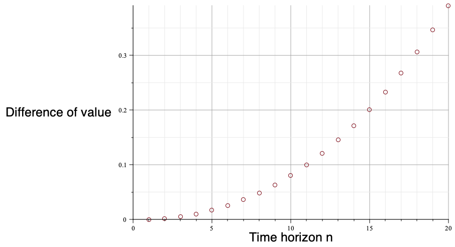
The difference of the two values for the single-asset case and different time horizons is given in Figure 1. We present a stationary model with two-point distribution of $\tilde{R}$ given by $\mathbb{P}(\tilde{R}=1+4i)=\mathbb{P}(\tilde{R}=1-i)=\frac{1}{2},$ where $i$ is an interest rate in each period, and $\lambda=1.$ In this case, $\ell=\frac{1}{26}$ and the difference does not depend on $i$. For $N=1$, the two-values coincide. However, the difference gets larger, the larger the time-horizon is. Thus, the equilibrium strategy is suboptimal for $P(\lambda),$ although is found by backward induction. Since it is suboptimal, it is not time-consistent according to Definition 2.1.

Refer to caption
Figure 1. Difference of target values under the optimal policy and the equilibrium strategy for a stationary model with $\ell=1/26$ for different time horizons.

2.4. Solution 3: Population version

In this part, we show that the solution obtained in Proposition 2.2 can be seen as a time-consistent solution provided that we enlarge the state space. More precisely, the idea relies on replacing the state space $E$ by the set of probability measures on $E.$ In this way, the problem becomes purely deterministic and more importantly, as can be seen below, the Bellman principle holds. The advantage of our approach is that we can solve the problem directly as an MDP without making use of any auxiliary problem. Using backward induction we obtain a time-consistent policy for the investor in this population version model.

In our new setting, a population version MDP is defined by the following items:

  • $\hat{E}:=\Pr(E)$ is the state space, where $\mu\in\hat{E}$ denotes the distribution of the wealth,

  • $\hat{A}:=F$ is the action space, where $\phi\in\hat{A}$ is the decision rule to be applied,

  • $\hat{T}_{n}(\mu,\phi)=\mu^{\prime}$ is the transition function, where

    $$\mu^{\prime}(B)=\int\mathbb{P}\big{(}(1+i_{n+1})(x+\phi(x)\cdot R_{n+1})\in B\big{)}\mu(dx)=\int Q_{n}^{\phi}(B|x)\mu(dx)$$

    for a Borel set $B\subset E,$ where $Q_{n}^{\phi}(B|x):=Q_{n}(B|x,\phi(x)),$ $x\in E;$ alternatively, $\mu^{\prime}=\mathcal{L}\big{(}(1+i_{n+1})(X+\phi(X)\cdot R_{n+1})\big{)}$ with $X\sim\mu$ independent of $R_{n+1}$,

  • $\hat{c}_{N}(\mu)=\int(x^{2}-2\lambda x)\mu(dx)-\Big{(}\int x\mu(dx)\Big{)}^{2}$ is the terminal cost.

The transition functions $\hat{T}_{n}$ are purely deterministic, which implies that this problem can be seen as a deterministic dynamic program. Without loss of generality, we restrict to the Markovian decision rules $\hat{\phi}_{n}\in\hat{F}$, where

$$\hat{F}:=\{\hat{\phi}:\hat{E}\to\hat{A}\}.$$

We place no measurability requirements on these mappings.

The aim is now to solve

$$\hat{P}(\lambda)\left\{\begin{array}[]{l}Var_{\mu_{0}}^{\pi}[X_{N}]-2\lambda\mathbb{E}_{\mu_{0}}^{\pi}[X_{N}]\to\inf\\ \pi\in\Pi\end{array}\right.$$

This means that the variance and expectation are taken w.r.t. the product measure $\mathbb{P}_{\mu_{0}}^{\pi}$ defined by $\mu_{0}$ and the transition kernels of $(X_{n})$ generated by the policy $\pi=(\pi_{0},\ldots,\pi_{N-1}).$ Clearly, the problem $\hat{P}(\lambda)$ becomes non-trivial if $N\geq 2.$

Observe that the initial capital is drawn at random at the beginning, i.e., $X_{0},$ is not deterministic, but has a distribution $\mu_{0}$. In case $\mu_{0}=\delta_{x_{0}},$ the problem reduces to the initial problem $P(\lambda).$ An alternative interpretation is that we consider a continuum of agents with wealth distributed according to $\mu_{0}.$

Definition 2.5.

For a fixed policy $\hat{\pi}=(\hat{\phi}_{0},\ldots,\hat{\phi}_{N-1})$ define

$\displaystyle\phi_{0}$ $\displaystyle:=\hat{\phi}_{0}(\mu_{0}),\quad\mu_{1}:=\hat{T}_{0}(\mu_{0},\phi_{0}),$
$\displaystyle\phi_{1}$ $\displaystyle:=\hat{\phi}_{1}(\mu_{1}),\quad\mu_{2}:=\hat{T}_{1}(\mu_{1},\phi_{1}),$
$\displaystyle\vdots$
$\displaystyle\phi_{N-1}$ $\displaystyle:=\hat{\phi}_{N-1}(\mu_{N-1}),\quad\mu_{N}:=\hat{T}_{N-1}(\mu_{N-1},\phi_{N-1}).$ (2.6)

The sequence of actions defines a policy $\pi=(\phi_{0},\phi_{1},\ldots,\phi_{N-1})$ in the original problem formulation.

From this definition we immediately have:

Lemma 2.6.

Under policy $\hat{\pi}=(\hat{\phi}_{0},\ldots,\hat{\phi}_{N-1})$, the distribution of $X_{k}$ is equal to $\mu_{k}$, where $\mu_{k}$ are defined in (2.6) for $k=0,1,\ldots,N.$

Proof.

The proof is by induction. For $k=0,$ the statement is obvious. Suppose that $X_{k}\sim\mu_{k}$ for $k=1,\ldots,n.$ Then,

$$\mu_{n+1}=\hat{T}_{n}(\mu_{n},\hat{\phi}_{n}(\mu_{n}))=\hat{T}_{n}(\mu_{n},\phi_{n})=\int\mathbb{P}\big{(}(1+i_{n+1})(x+\phi_{n}(x)\cdot R_{n+1})\in\bullet\big{)}\mu_{n}(dx).$$

By construction, the distribution of $X_{n+1}$ is given by $\mu_{n+1}.$ This implies the result. ∎

Next for a fixed policy $\hat{\pi}=(\hat{\phi}_{0},\ldots,\hat{\phi}_{N-1})$ define

$\displaystyle J_{N,\hat{\pi}}(\mu)$ $\displaystyle:=$ $\displaystyle\hat{c}_{N}(\mu),$
$\displaystyle\mbox{and}\quad J_{n,\hat{\pi}}(\mu)$ $\displaystyle:=$ $\displaystyle J_{n+1,\hat{\pi}}(\hat{T}_{n}(\mu,\hat{\phi}_{n}(\mu)))\quad\mbox{for }n=1,\ldots,N.$

Then, again making use of induction we obtain:

Lemma 2.7.

Under policy $\hat{\pi}=(\hat{\phi}_{0},\ldots,\hat{\phi}_{N-1})$,

$$J_{0,\hat{\pi}}(\mu_{0})=Var_{\mu_{0}}^{\pi}[X_{N}]-2\lambda\mathbb{E}_{\mu_{0}}^{\pi}[X_{N}],$$

where $\pi$ on the right-hand side is defined as in (2.6).

Proof.

Indeed, note that

$$J_{0,\hat{\pi}}(\mu_{0})=J_{1,\hat{\pi}}(\hat{T}_{0}(\mu_{0},\hat{\phi}_{0}(\mu_{0})))=J_{1,\hat{\pi}}(\mu_{1})=\ldots=J_{N,\hat{\pi}}(\mu_{N})\\ =\hat{c}_{N}(\mu_{N}).$$

The claim now follows from the definition of $\hat{c}_{N}$ and Lemma 2.6. ∎

Finally, we define for $n=0,\ldots,N-1$:

$\displaystyle J_{N}(\mu)$ $\displaystyle:=\hat{c}_{N}(\mu),$
$\displaystyle J_{n}(\mu)$ $\displaystyle:=\inf_{\hat{\phi}\in\hat{F}}J_{n+1}(\hat{T}_{n}(\mu,\hat{\phi}(\mu))).$ (2.7)

If the minimum in (2.7) is attained, we denote it by $\hat{\phi}^{*}_{n}(\mu).$ Using backward induction, we get the following result.

Theorem 2.8.
  • (i)

    If the initial distribution is $\mu_{0},$ then the value of the problem $\hat{P}(\lambda)$ is $J_{0}(\mu_{0})$ and

    $$J_{0}(\mu_{0})=(S^{0}_{N})^{2}d_{0}\Big{(}\int x^{2}\mu_{0}(dx)-\big{(}\int x\mu_{0}(dx)\big{)}^{2}\Big{)}-2\lambda S_{N}^{0}\int x\mu_{0}(dx)-\lambda^{2}\Big{(}\frac{1}{d_{0}}-1\Big{)}.$$
  • (ii)

    The optimal policy in the population version model is given by $\hat{\pi}^{*}=(\hat{\phi}^{*}_{0},\ldots,\hat{\phi}^{*}_{N-1})$, where

    $$\hat{\phi}^{*}_{n}(\nu)(x)=\left(\frac{\lambda S^{0}_{n}}{d_{n}S^{0}_{N}}+\int x^{\prime}\nu(dx^{\prime})-x\right)C_{n+1}^{-1}\mathbb{E}R_{n+1},$$

    for $n=0,\ldots,N-1,$ $\nu\in\hat{E}$ and $x\in E.$

Proof.

We wish to find an optimal decision rule $\hat{\phi}^{*}_{N-1}$ at time point $N-1.$ Let $X_{N-1}\sim\nu.$ Then,

$\displaystyle J_{N-1}(\nu)=$ $\displaystyle\inf_{\hat{\phi}\in\hat{F}}J_{N}(\hat{T}_{N-1}(\nu,\hat{\phi}(\nu)))=\inf_{\phi\in F}\hat{c}_{N}(\hat{T}_{N-1}(\nu,\phi))$
$\displaystyle=$ $\displaystyle\inf_{\phi\in F}\left(\mathbb{E}_{N,\hat{T}_{N-1}(\nu,\phi)}\Big{[}(X_{N})^{2}-2\lambda X_{N}\Big{]}-\Big{(}\mathbb{E}_{N,\hat{T}_{N-1}(\nu,\phi)}[X_{N}]\Big{)}^{2}\right)$ (2.8)
$\displaystyle=$ $\displaystyle(1+i_{N})^{2}\inf_{\phi\in F}\mathbb{E}_{N-1,\nu}\Big{[}(X_{N-1}+\phi(X_{N-1})\cdot R_{N})^{2}+$
$\displaystyle-\frac{2\lambda}{1+i_{N}}(X_{N-1}+\phi(X_{N-1})\cdot R_{N})-\Big{(}\mathbb{E}_{N-1,\nu}\Big{[}X_{N-1}+\phi(X_{N-1})\cdot R_{N}\Big{]}\Big{)}^{2}\Big{]}.$

We use here the notation $\mathbb{E}_{n,\nu}$ to indicate that we start at the time point $n$ and the random variable $X_{n}$ has distribution $\nu.$ In case $n=0,$ we simply write $\mathbb{E}_{\nu}.$ By Appendix 7.1 the solution of the problem is

$$\hat{\phi}^{*}_{N-1}(\nu)(x)=\left(\frac{\lambda S_{N-1}^{0}}{d_{N-1}S_{N}^{0}}+\int x^{\prime}\nu(dx^{\prime})-x\right)C_{N}^{-1}\mathbb{E}R_{N}.$$

This also implies that

$\displaystyle J_{N-1}(\nu)$ $\displaystyle=$ $\displaystyle d_{N-1}\Big{(}\frac{S_{N}^{0}}{S_{N-1}^{0}}\Big{)}^{2}\Big{(}\mathbb{E}_{N-1,\nu}[X_{N-1}^{2}]-(\mathbb{E}_{N-1,\nu}[X_{N-1}])^{2}+$
$\displaystyle\hskip 85.35826pt-\frac{2\lambda}{d_{N-1}S_{N}^{0}/S_{N-1}^{0}}\mathbb{E}_{N-1,\nu}[X_{N-1}]\Big{)}-\lambda^{2}\frac{\ell_{N}}{1-\ell_{N}}.$

At time $N-2$ the expression which has to be minimized is the same as at time $N-1,$ when we replace $\lambda$ by $\frac{\lambda S^{0}_{N-1}}{d_{N-1}S^{0}_{N}}$ in (2.4). Indeed, observe that

$\displaystyle J_{N-2}(\nu)$ $\displaystyle=$ $\displaystyle\inf_{\phi\in F}J_{N-1}(\hat{T}_{N-2}(\nu,\phi))$
$\displaystyle=$ $\displaystyle d_{N-1}\Big{(}\frac{S_{N}^{0}}{S_{N-1}^{0}}\Big{)}^{2}\inf_{\phi\in F}\Big{(}\mathbb{E}_{N-1,\hat{T}_{N-2}(\nu,\phi)}[X_{N-1}^{2}]-(\mathbb{E}_{N-1,\hat{T}_{N-2}(\nu,\phi)}[X_{N-1}])^{2}+$
$\displaystyle\hskip 28.45274pt-\frac{2\lambda}{d_{N-1}S_{N}^{0}/S_{N-1}^{0}}\mathbb{E}_{N-1,\hat{T}_{N-2}(\nu,\phi)}[X_{N-1}]\Big{)}-\lambda^{2}\frac{\ell_{N}}{1-\ell_{N}}.$

We obtain

$\displaystyle\hat{\phi}^{*}_{N-2}(\nu)(x)$ $\displaystyle=$ $\displaystyle\left(\frac{\lambda S^{0}_{N-2}}{d_{N-2}S^{0}_{N}}+\int x^{\prime}\nu(dx^{\prime})-x\right)C_{N-1}^{-1}\mathbb{E}R_{N-1}$

and

$\displaystyle J_{N-2}(\nu)$ $\displaystyle=$ $\displaystyle d_{N-2}\Big{(}\frac{S_{N}^{0}}{S_{N-2}^{0}}\Big{)}^{2}\Big{(}\mathbb{E}_{N-2,\nu}[X_{N-2}^{2}]-(\mathbb{E}_{N-2,\nu}[X_{N-2}])^{2}$
$\displaystyle-\frac{2\lambda}{d_{N-2}S_{N}^{0}/S_{N-2}^{0}}\mathbb{E}_{N-2,\nu}[X_{N-2}]\Big{)}-\lambda^{2}\left(\frac{\ell_{N}}{1-\ell_{N}}+\frac{\ell_{N-1}}{(1-\ell_{N-1})(1-\ell_{N})}\right).$

Continuing this procedure we finally get

$$\hat{\phi}^{*}_{0}(\nu)(x)=\left(\frac{\lambda}{d_{0}S^{0}_{N}}+\int x^{\prime}\nu(dx^{\prime})-x\right)C_{1}^{-1}\mathbb{E}R_{1}$$

and

$\displaystyle J_{0}(\nu)$ $\displaystyle=$ $\displaystyle d_{0}\Big{(}\frac{S_{N}^{0}}{S_{0}^{0}}\Big{)}^{2}\left(\mathbb{E}_{\nu}[X_{0}^{2}]-(\mathbb{E}_{\nu}[X_{0}])^{2}-\frac{2\lambda}{d_{0}S_{N}^{0}}\mathbb{E}_{\nu}[X_{0}]\right)+$
$\displaystyle-\lambda^{2}\left(\frac{\ell_{N}}{1-\ell_{N}}+\frac{\ell_{N-1}}{(1-\ell_{N})(1-\ell_{N-1})}+\ldots+\frac{\ell_{1}}{(1-\ell_{N})\cdots(1-\ell_{1})}\right)$
$\displaystyle=$ $\displaystyle d_{0}(S_{N}^{0})^{2}Var_{\nu}[X_{0}]-2\lambda S_{N}^{0}\mathbb{E}_{\nu}[X_{0}]-\lambda^{2}\left(\frac{1}{d_{0}}-1\right).$

Note that the last equality follows from

$\displaystyle\sum_{k=1}^{N}\frac{\ell_{k}}{(1-\ell_{N})\ldots(1-\ell_{k})}$ $\displaystyle=$ $\displaystyle\sum_{k=1}^{N}\frac{\ell_{k}}{d_{k-1}}=\sum_{k=1}^{N}\frac{d_{k}-d_{k-1}}{d_{k-1}d_{k}}$
$\displaystyle=$ $\displaystyle\sum_{k=1}^{N}\Big{(}\frac{1}{d_{k-1}}-\frac{1}{d_{k}}\Big{)}=\frac{1}{d_{0}}-\frac{1}{d_{N}}=\frac{1}{d_{0}}-1.$

Hence, we have defined the optimal policy $\hat{\pi}^{*}=(\hat{\phi}^{*}_{0},\ldots,\hat{\phi}^{*}_{N-1}).$ Now, if $\mu_{0}$ is an initial distribution, then $J_{0}(\mu_{0})$ is optimal value for $\hat{P}(\lambda).$

The policy $\hat{\pi}^{*}$ obtained in Theorem 2.8 is time-consistent in the population version model due to Definition 2.1. This is because the same functions $J_{n}$ and $J_{n+1}$ appear on the left-hand and right-hand side in (2.7). This immediately implies that the Bellman optimality principle holds and backward induction in this case produces an optimal policy.

Assume that $\mu_{0}\in\hat{E}$ is given. Then, making use of $\hat{\pi}^{*}$ according to (2.6) we may define a policy $\pi^{*}=(\phi^{*}_{0},\ldots,\phi^{*}_{N-1})$ for the original mean-variance model and the measures $\mu_{1},\ldots,\mu_{N}.$ More precisely, $\phi^{*}_{n}=\hat{\phi}^{*}_{n}(\mu_{n})$ where $\mu_{n}$ is the distribution of the $n$-th state and

$$\phi^{*}_{n}(x)=\left(\frac{\lambda S^{0}_{n}}{d_{n}S^{0}_{N}}+\int x^{\prime}\mu_{n}(dx^{\prime})-x\right)C_{n+1}^{-1}\mathbb{E}R_{n+1},\quad x\in E,$$ (2.9)

$n=0,\ldots,N-1.$

Corollary 2.9.

If $\mu_{0}=\delta_{x_{0}},$ then the value $J_{0}(\delta_{x_{0}})$ is the value of $P(\lambda)$ and $J_{0}(\delta_{x_{0}})=V^{o}(x_{0}).$ The policy $\pi^{*}=(\phi^{*}_{0},\ldots,\phi^{*}_{N-1})$ with $\phi^{*}_{n}$ defined in (2.9) for $n=0,\ldots,N-1$ is optimal. These decision rules are history-dependent, however depend at time $n$ on the history only through $\mu_{n}.$

Furthermore, we observe that the expression $\int x^{\prime}\mu_{n}(dx^{\prime})$ in (2.9) is exactly $\mathbb{E}_{\mu_{0}}^{\pi^{*}}[X_{n}].$ Thus, we can compute it as follows:

$\displaystyle\mathbb{E}_{\mu_{0}}^{\pi^{*}}[X_{1}]$ $\displaystyle=(1+i_{1})\mathbb{E}_{\mu_{0}}\Big{[}X_{0}+\phi_{0}^{*}(X_{0})\cdot R_{1}\Big{]}=(1+i_{1})\Big{(}\mathbb{E}_{\mu_{0}}[X_{0}]+\frac{\lambda}{d_{0}S_{N}^{0}}\ell_{1}\Big{)}$
$\displaystyle=S_{1}^{0}\Big{(}\mathbb{E}_{\mu_{0}}[X_{0}]+\frac{\lambda}{S_{N}^{0}}\frac{\ell_{1}}{d_{0}}\Big{)}.$

For arbitrary time $n=1,\ldots,N,$ we get

$$\mathbb{E}_{\mu_{0}}^{\pi^{*}}[X_{n}]=S_{n}^{0}\Big{(}\mathbb{E}_{\mu_{0}}[X_{0}]+\frac{\lambda}{S_{N}^{0}}\sum_{k=1}^{n}\frac{\ell_{k}}{d_{k-1}}\Big{)}.$$

Next we insert this in (2.9) to obtain for $n=0,\ldots,N-1$:

$\displaystyle\phi^{*}_{n}(x)$ $\displaystyle=$ $\displaystyle\left(S_{n}^{0}\mathbb{E}_{\mu_{0}}[X_{0}]+\lambda\frac{S^{0}_{n}}{S^{0}_{N}}\Big{(}\sum_{k=1}^{n}\frac{\ell_{k}}{d_{k-1}}+\frac{1}{d_{n}}\Big{)}-x\right)C_{n+1}^{-1}\mathbb{E}R_{n+1}$ (2.10)
$\displaystyle=$ $\displaystyle\left(\Big{(}\mathbb{E}_{\mu_{0}}[X_{0}]+\frac{\lambda}{S^{0}_{N}d_{0}}\Big{)}S_{n}^{0}-x\right)C_{n+1}^{-1}\mathbb{E}R_{n+1},\quad x\in E,$

since for all $n=1,\ldots,N-1$:

$$\sum_{k=1}^{n}\frac{\ell_{k}}{d_{k-1}}+\frac{1}{d_{n}}=\sum_{k=1}^{n}\Big{(}\frac{1}{d_{k-1}}-\frac{1}{d_{k}}\Big{)}+\frac{1}{d_{n}}=\frac{1}{d_{0}}.$$

Thus, if we consider $\mu_{0}=\delta_{0},$ then the optimal policy in (2.10) coincides with the optimal policy $\pi^{o}$ in Proposition 2.2. Moreover, the optimal values are the same, i.e., the use of further information does not improve the value. Comparing the two approaches we may point out two advantages for the latter one. First, we were able to solve our problem $P(\lambda)$ directly without using auxiliary problems. We need only forward recursion formulae in Definition 2.5. Second, in the population version model, this policy can be viewed as time-consistent, i.e., it is optimal and satisfies the Bellman optimality principle.

Compared to the second solution with the equilibrium strategy $\pi^{e}$, it is already clear by construction that the value obtained in the population version MDP cannot be worse. This is because the policy in (2.9) can be seen as a history-dependent policy in the original formulation. This policy depends on the process history only via the probability distribution, i.e., $\mu_{n}$ is a function of $(X_{0},A_{0},\ldots,A_{n-1}).$ The equilibrium strategy, on the other hand, is completely deterministic.

3. General non-additive Markov decision processes

In this section, we consider a generalization of the mean-variance problem. We show that a general time-inconsistent problem can be solved yielding a time-consistent policy in the population version MDP. Suppose we are given an original MDP with finite time horizon $N$ and with the following data:

  • $(E,\mathcal{B}(E))$ is a Borel state space; the states are denoted by $x\in E,$

  • $(A,\mathcal{B}(A))$ is a Borel action space; the actions are denoted by $a\in A$,

  • $(\mathcal{R},\mathcal{B}(\mathcal{R}))$ is some Borel space; the random variables $R_{1},\ldots,R_{N}$ are independent with values in $\mathcal{R}$ defined on the joint probability space $(\Omega,\mathcal{F},\mathbb{P})$,

  • $T_{n}(x,a,r)$ is a measurable transition function at time $n=0,\ldots,N-1$, i.e., $T_{n}:E\times A\times\mathcal{R}\to E$ and

    $$X_{n+1}=T_{n}(X_{n},A_{n},R_{n+1})$$

    is the new state at time $n+1,$ given the state at time $n$ is $X_{n}$ and action $A_{n}$ is taken; then

    $$Q_{n}(B|x,a)=\mathbb{P}\big{(}T_{n}(x,a,R_{n+1})\in B\big{)},\quad B\in\mathcal{B}(E)$$

    is the transition kernel,

  • $c_{n}(x,a)$ is a measurable cost function $c_{n}:E\times A\to\mathbb{R},$ which gives the cost at time $n=0,\ldots,N-1$ in state $x$ and action $a$,

  • $c_{N}(x)$ is the terminal cost in state $x$, i.e., $c_{N}:E\to\mathbb{R}$,

  • $h:E\to\mathbb{R}$ and $G:\mathbb{R}\to\mathbb{R}$ are measurable functions providing the non-additivity. We set $G(\infty):=\infty.$

In what follows, let $\Pi$ be the set of all deterministic history-dependent policies $\pi=(\pi_{0},\ldots,\pi_{N-1}),$ i.e., if $h_{n}=(x_{0},a_{0},\ldots,x_{n})$ is the history up to time $n$, then $\phi_{n}(h_{n})$ gives the action at time $n$. By

$$F:=\{\phi:E\to A\ |\ \phi\mbox{ is measurable}\}$$

we denote the set of Markovian decision rules. We are now interested in minimizing the following $N$-stage cost over all history-dependent policies:

$$\mathbb{E}_{x_{0}}^{\pi}\Big{[}\sum_{k=0}^{N-1}c_{k}(X_{k},A_{k})+c_{N}(X_{N})\Big{]}+G(\mathbb{E}_{x_{0}}^{\pi}[h(X_{N})])\to\inf_{\pi\in\Pi}$$ (3.1)

If $G$ is linear then this problem is a standard MDP and we can solve it with established techniques (see Remark 3.5). In what follows, we make no specific assumption about $G.$ In order to have a well-defined problem, we assume that a lower bounding function exists, i.e., there exists a measurable mapping $b:E\to\mathbb{R}$ and constants $\bar{c}_{n},\bar{c}_{h},\bar{c}_{N},\alpha_{b}>0$ such that

  • (i)

    $c_{n}^{-}(x,a)\leq\bar{c}_{n}b(x)$ for all $(x,a)\in E\times A,n=0,\ldots,N-1$,

  • (ii)

    $c_{N}^{-}(x)\leq\bar{c}_{N}b(x)$ for all $x\in E$,

  • (iii)

    $h^{-}(x)\leq\bar{c}_{h}b(x)$ for all $x\in E$,

  • (iv)

    $\int b(x^{\prime})Q^{\phi}(dx^{\prime}|x)\leq\alpha_{b}b(x)$ for all $x\in E$ and decision rules $\phi$,

where $a^{-}=-\min\{0,a\},$ $a\in\mathbb{R}.$ This implies that all expectations are well-defined. We solve the problem again as a population version MDP:

  • $\hat{E}:=\mathbb{P}(E)$ is the state space, where $\mu\in\hat{E}$ is a probability measure on $E$,

  • $\hat{A}:=F$ is the action space, where $\phi\in\hat{A}$ is a decision rule for the original MDP,

  • $\hat{T}_{n}(\mu,\phi)=\mu^{\prime}$ is the transition function, where

    $\displaystyle\mu^{\prime}(B)$ $\displaystyle=\int\mathbb{P}\big{(}T_{n}(x,\phi(x),R_{n+1})\in B\big{)}\mu(dx)$
    $\displaystyle=\int Q_{n}(B|x,\phi(x))\mu(dx)=\int Q_{n}^{\phi}(B|x)\mu(dx)$

    and $Q_{n}^{\phi}(B|x)=Q_{n}(B|x,\phi(x)),$ for $B\in\mathcal{B}(E)$ and $x\in E$,

  • $\hat{c}_{n}(\mu,\phi)=\int c_{n}(x,\phi(x))\mu(dx)$ is the one-stage cost,

  • $\hat{c}_{N}(\mu)=\int c_{N}(x)\mu(dx)+G(\int h(x)\mu(dx))$ is the terminal cost.

This MDP is now a deterministic dynamic program. We know that we can restrict the optimization to Markovian policies $\hat{\pi}=(\hat{\phi}_{0},\ldots,\hat{\phi}_{N-1}),$ where each $\hat{\phi}_{n}\in\hat{F}$ for $n=0,\ldots,N-1,$ and $\hat{F}=\{\hat{\phi}:\hat{E}\to\hat{A}\}.$ We again do not require any measurability conditions of the mappings in $\hat{F}.$

Definition 3.1.

Given a policy $\hat{\pi}=(\hat{\phi}_{0},\ldots,\hat{\phi}_{N-1})$ we obtain the following state-action sequence:

$\displaystyle\phi_{0}$ $\displaystyle:=\hat{\phi}_{0}(\mu_{0}),\quad\mu_{1}:=\hat{T}_{0}(\mu_{0},\phi_{0}),$
$\displaystyle\phi_{1}$ $\displaystyle:=\hat{\phi}_{1}(\mu_{1}),\quad\mu_{2}:=\hat{T}_{1}(\mu_{1},\phi_{1}),$
$\displaystyle\vdots$
$\displaystyle\phi_{N-1}$ $\displaystyle:=\hat{\phi}_{N-1}(\mu_{N-1}),\quad\mu_{N}:=\hat{T}_{N-1}(\mu_{N-1},\phi_{N-1}).$ (3.2)

The sequence of actions defines a policy $\pi=(\phi_{0},\phi_{1},\ldots,\phi_{N-1})$ in the original MDP.

Lemma 3.2.

Under policy $\hat{\pi}=(\hat{\phi}_{0},\ldots,\hat{\phi}_{N-1})$, the distribution of $X_{k}$ is equal to $\mu_{k}$, where $\mu_{k}$ are defined in (3.2) for $k=0,1,\ldots,N.$

Proof.

The proof goes by induction as in Lemma 2.6 with the obvious changes. ∎

The value functions for a fixed policy $\hat{\pi}=(\hat{\phi}_{0},\ldots,\hat{\phi}_{N-1})$ are given by

$\displaystyle J_{N,\hat{\pi}}(\mu)$ $\displaystyle:=$ $\displaystyle\hat{c}_{N}(\mu),$
$\displaystyle\mbox{and}\quad J_{n,\hat{\pi}}(\mu)$ $\displaystyle:=$ $\displaystyle\hat{c}_{n}(\mu,\hat{\phi}_{n}(\mu))+J_{n+1,\hat{\pi}}(\hat{T}_{n}(\mu,\hat{\phi}_{n}(\mu))),\quad n=0,\ldots,N-1.$
Lemma 3.3.

Under policy $\hat{\pi}=(\hat{\phi}_{0},\ldots,\hat{\phi}_{N-1})$,

$$J_{0,\hat{\pi}}(\mu_{0})=\mathbb{E}_{\mu_{0}}^{\pi}\Big{[}\sum_{k=0}^{N-1}c_{k}(X_{k},A_{k})+c_{N}(X_{N})\Big{]}+G(\mathbb{E}_{\mu_{0}}^{\pi}[h(X_{N})]),$$

where $\pi$ on the right-hand side is defined as in (3.2).

Proof.

We obtain

$\displaystyle J_{0,\hat{\pi}}(\mu_{0})$ $\displaystyle=$ $\displaystyle\hat{c}_{0}(\mu_{0},\hat{\phi}_{0}(\mu_{0}))+J_{1,\hat{\pi}}(\hat{T}_{0}(\mu_{0},\hat{\phi}_{0}(\mu_{0})))=\hat{c}_{0}(\mu_{0},\phi_{0})+J_{1,\hat{\pi}}(\hat{T}_{0}(\mu_{0},\phi_{0}))$
$\displaystyle=$ $\displaystyle\mathbb{E}_{\mu_{0}}[c_{0}(X_{0},\phi_{0}(X_{0}))]+J_{1,\hat{\pi}}(\mu_{1})$
$\displaystyle=$ $\displaystyle\mathbb{E}_{\mu_{0}}[c_{0}(X_{0},\phi_{0}(X_{0}))]+\mathbb{E}_{1,\mu_{1}}[c_{1}(X_{1},\phi_{1}(X_{1}))]+J_{2,\hat{\pi}}(\hat{T}_{1}(\mu_{1},\phi_{1}))$
$\displaystyle=$ $\displaystyle\mathbb{E}_{\mu_{0}}[c_{0}(X_{0},\phi_{0}(X_{0}))]+\ldots+\mathbb{E}_{N-1,\mu_{N-1}}[c_{N-1}(X_{N-1},\phi_{N-1}(X_{N-1}))]+\hat{c}_{N}(\mu_{N})$
$\displaystyle=$ $\displaystyle\mathbb{E}_{\mu_{0}}^{\pi}\Big{[}\sum_{k=0}^{N-1}c_{k}(X_{k},\phi_{k}(X_{k}))+c_{N}(X_{N})\Big{]}+G(\mathbb{E}_{\mu_{0}}^{\pi}[h(X_{N})]),$

where we have used Lemma 3.2 and (3.2). ∎

Finally, we define for $n=1,\ldots,N$:

$\displaystyle J_{N}(\mu)$ $\displaystyle:=\hat{c}_{N}(\mu),$
$\displaystyle J_{n}(\mu)$ $\displaystyle:=\inf_{\hat{\phi}\in\hat{F}}\left(\hat{c}_{n}(\mu,\hat{\phi}(\mu))+J_{n+1}(\hat{T}_{n}(\mu,\hat{\phi}(\mu)))\right).$ (3.3)

If the minimum in (3.3) is attained, we denote it by $\hat{\phi}_{n}^{*}(\mu).$ Note that the recursion in (3.3) is exactly the standard Bellman equation, because on the right-hand we have the sum of the current cost and the value function, whereas on the left hand side we have the same value function. This means that the optimal policy in the population version MDP (if it exists) is time-consistent according to Definition 2.1. Thus, we obtain as in the previous section:

Theorem 3.4.

Assume that the initial distribution is $\mu_{0}=\delta_{x_{0}}.$ The value $J_{0}(\mu_{0})$ obtained with the recursion in (3.3) is the value of problem (3.1) and the optimal policy (if it exists) $\hat{\pi}^{*}=(\hat{\phi}^{*}_{0},\ldots,\hat{\phi}^{*}_{N-1})$ is time-consistent in the population version MDP. The policy $\pi^{*}=(\phi^{*}_{0},\ldots,\phi^{*}_{N-1})$ defined in (3.2), i.e., $\phi^{*}_{k}=\hat{\phi}^{*}_{k}(\mu_{k})$ for $k=0,\ldots,N-1$ is optimal in the original formulation. These decision rules are history-dependent, however depend at time $n$ on the history only through $\mu_{n}$.

Theorem 3.4 means that the optimal policy in the original formulation can be computed by a backward-forward algorithm. First, we use (3.3) to determine the value functions $J_{n}$ and the optimal policy $\hat{\pi}^{*}.$ Then, we use (3.2) to find the sequence of measures $\mu_{0},\ldots,\mu_{N-1}$ and the policy $\pi^{*}$.

Remark 3.5.

In case $G(x)=x$ (w.l.o.g. we can then set $c_{N}\equiv 0$) and in case minimizers exist, our solution method boils down to the classical Bellman equations of MDP theory. Indeed, in this case it can be shown by induction that $J_{n}(\mu)=\int V_{n}(x)\mu(dx),n=0,1,\ldots,N$ for some measurable functions $V_{n}.$ The proof is as follows. First, for $N$ we have by definition $J_{N}(\mu)=\int h(x)\mu(dx)$. Suppose $J_{n+1}(\mu)=\int V_{n+1}(x)\mu(dx).$ Then

$\displaystyle J_{n}(\mu)$ $\displaystyle=\inf_{\phi\in F}\left(\int c_{n}(x,\phi(x))\mu(dx)+\int\mathbb{E}\big{[}V_{n+1}(T(x,\phi(x),R_{n+1}))\big{]}\mu(dx)\right)$
$\displaystyle=\inf_{\phi\in F}\left(\int c_{n}(x,\phi(x))+\mathbb{E}\big{[}V_{n+1}(T(x,\phi(x),R_{n+1}))\big{]}\mu(dx)\right)$
$\displaystyle=\int c_{n}(x,\phi^{*}(x))+\mathbb{E}\big{[}V_{n+1}(T(x,\phi^{*}(x),R_{n+1}))\big{]}\mu(dx)$

which implies the statement. Note that, in particular, the minimization can be done pointwise, which yields the classical Bellman equation

$$V_{n}(x)=\inf_{\phi\in F}\Big{(}c_{n}(x,\phi(x))+\mathbb{E}\big{[}V_{n+1}(T(x,\phi(x),R_{n+1}))\big{]}\Big{)}.$$

4. Application: LQ-problem

In this section, we apply our findings to the following LQ-problem considered in [6], Sec. 9:

$$\mathbb{E}_{\mu_{0}}^{\pi}\Big{[}\sum_{k=0}^{N-1}A_{k}^{2}\Big{]}+(\mathbb{E}_{\mu_{0}}^{\pi}[X_{N}])^{2}\to\inf_{\pi}$$ (4.1)

where the next state evolves according to the equation

$$X_{n+1}=bX_{n}+dA_{n}+\sigma R_{n+1}.$$

Here $X_{n}\in E=\mathbb{R},$ $A_{n}\in A=\mathbb{R}$ and $R_{1},\ldots,R_{N}$ are i.i.d. random variables with a finite second moment and $\mathbb{E}R_{n}=0$ for $n=1,\ldots,N$, $b,d\in\mathbb{R},$ $\sigma>0.$ Hence, within this framework in the population version MDP, the transition function is $\hat{T}_{n}(\mu,\phi)=\mu^{\prime},$ where

$$\mu^{\prime}(B)=\int\mathbb{P}(T_{n}(x,\phi(x),R_{n+1})\in B)\mu(dx)=\int\mathbb{P}(bx+d\phi(x)+\sigma R_{n+1}\in B)\mu(dx)$$

for a Borel set $B\subset E.$ Moreover,

$$\hat{c}_{n}(\mu,\phi)=\int\phi(x)^{2}\mu(dx)$$

is the one-stage cost, whereas

$$\hat{c}_{N}(\mu)=\Big{(}\int x\mu(dx)\Big{)}^{2}$$

is the terminal cost.

In order to solve the problem, we first consider the final time point, where

$$J_{N}(\nu)=\Big{(}\int x\nu(dx)\Big{)}^{2}=\Big{(}\mathbb{E}_{N,\nu}[X_{N}]\Big{)}^{2}.$$

At time point $N-1,$ equation (3.3) becomes

$\displaystyle J_{N-1}(\nu)$ $\displaystyle=\inf_{\phi\in F}\left(\mathbb{E}_{N-1,\nu}[\phi^{2}(X_{N-1})]+J_{N}(\hat{T}_{N-1}(\nu,\phi))\right)$
$\displaystyle=\inf_{\phi\in F}\left(\mathbb{E}_{N-1,\nu}[\phi^{2}(X_{N-1})]+\Big{(}b\mathbb{E}_{N-1,\nu}[X_{N-1}]+d\mathbb{E}_{N-1,\nu}[\phi(X_{N-1})]\Big{)}^{2}\right).$

The minimizer is given by (see Appendix 7.2)

$$\hat{\phi}^{*}_{N-1}(\nu)(x)=-\frac{bd}{1+d^{2}}\mathbb{E}_{N-1,\nu}[X_{N-1}],\quad\nu\in\hat{E},\ x\in E.$$

Plugging this minimizer into the equation for $J_{N-1}$ we obtain:

$$J_{N-1}(\nu)=\frac{b^{2}}{1+d^{2}}\Big{(}\mathbb{E}_{N-1,\nu}[X_{N-1}]\Big{)}^{2}.$$

Thus, we get again a quadratic form. Using the results in Appendix 7.2, it can be shown by induction that the optimal policy and value functions are given for $\nu\in\hat{E}$ by

$\displaystyle\hat{\phi}^{*}_{n}(\nu)(x)$ $\displaystyle=-\frac{bd\beta_{n+1}}{1+d^{2}\beta_{n+1}}\mathbb{E}_{n,\nu}[X_{n}],\quad x\in E,$ (4.2)
$\displaystyle J_{n}(\nu)$ $\displaystyle=\beta_{n}\big{(}\mathbb{E}_{n,\nu}[X_{n}]\big{)}^{2},$

where the constants $\beta_{n}$ are determined by the backward recursion

$$\beta_{N}=1,\quad\quad\beta_{n}=\frac{\beta_{n+1}b^{2}}{1+d^{2}\beta_{n+1}}.$$

Hence, making use of Theorem 3.4 we conclude:

Proposition 4.1.

If the initial distribution $\mu_{0}=\delta_{x_{0}},$ then $J_{0}(\mu_{0})=\beta_{0}x_{0}^{2}$ is the value of problem (4.1) and the optimal policy $\hat{\pi}^{*}=(\hat{\phi}^{*}_{0},\ldots,\hat{\phi}^{*}_{N-1})$ defined in (4.2) is time-consistent in the population version MDP. The policy $\pi^{*}=(\phi^{*}_{0},\ldots,\phi^{*}_{N-1})$ defined as in (4.2), i.e.,

$$\phi^{*}_{n}(x)=\hat{\phi}^{*}_{n}(\mu_{n})(x)\equiv-\frac{bd\beta_{n+1}}{1+d^{2}\beta_{n+1}}\mathbb{E}_{\mu_{n}}[X_{n}],\quad x\in E,$$

for $n=0,\ldots,N-1$, is optimal in the original formulation.

Since the sequence of states (measures) evolves in a deterministic way, we can compute $\mathbb{E}_{\mu_{n}}[X_{n}]$ by a forward recursion as follows

$\displaystyle\mathbb{E}_{\mu_{1}}[X_{1}]$ $\displaystyle=\mathbb{E}_{\mu_{0}}[bX_{0}+d\phi_{0}(X_{0})]=b\mathbb{E}_{\mu_{0}}[X_{0}]-\frac{bd^{2}\beta_{1}}{1+d^{2}\beta_{1}}\mathbb{E}_{\mu_{0}}[X_{0}]=\mathbb{E}_{\mu_{0}}[X_{0}]\frac{b}{1+d^{2}\beta_{1}}$

and in general

$$\mathbb{E}_{\mu_{n}}[X_{n}]=\mathbb{E}_{\mu_{0}}[X_{0}]\frac{b^{n}}{\prod_{k=1}^{n}(1+d^{2}\beta_{k})}.$$

Thus, we get that (in case $\mu_{0}=\delta_{x_{0}}$)

$\displaystyle\phi^{*}_{n}(x)$ $\displaystyle=-\frac{b^{n+1}d\beta_{n+1}}{\prod_{k=1}^{n+1}(1+d^{2}\beta_{k})}\mathbb{E}_{\mu_{0}}[X_{0}]=-\frac{b^{n+1}d\beta_{n+1}}{\prod_{k=1}^{n+1}(1+d^{2}\beta_{k})}x_{0},\quad x\in E,$
$\displaystyle J_{n}(\mu_{n})$ $\displaystyle=\beta_{n}\Big{(}\mathbb{E}_{\mu_{0}}[X_{0}]\frac{b^{n}}{\prod_{k=1}^{n}(1+d^{2}\beta_{k})}\Big{)}^{2}=\beta_{n}\Big{(}x_{0}\frac{b^{n}}{\prod_{k=1}^{n}(1+d^{2}\beta_{k})}\Big{)}^{2}.$

Hence, the optimal policy in the original model is semi-Markov. Although it is independent of the current state, it does depend on the initial state.

We now compare our solution to the equilibrium strategy given in [6], where the value function is computed by backward induction with the help of a system à la Bellman equations. For this approach we also have to assume that the variance of $R_{n}$ exist and is equal to 1. The value functions are of the form

$$V^{e}_{n}(x)=\beta_{n}x^{2}+\gamma_{n},\quad x\in E,$$

for $n=0,\ldots,N.$111There is a typo in the recursion for $A_{n}$ on p. 97 in [6]. In our setting, $A_{n}$ is exactly $\beta_{n}$. The constants $\gamma_{n}$ are computed recursively from $\gamma_{N}=0$ by

$$\gamma_{n}=\gamma_{n+1}+\sigma^{2}(\beta_{n+1}-\alpha_{n+1}^{2})$$

with $\alpha_{N}=1$ and

$\displaystyle\alpha_{n}$ $\displaystyle=\alpha_{n+1}\frac{b}{1+d^{2}\beta_{n+1}}.$

The equilibrium strategy is given by

$$\varphi_{n}(x)=-\frac{bd\beta_{n+1}}{1+d^{2}\beta_{n+1}}x,\quad x\in E,$$ (4.3)

for $n=0,\ldots,N-1.$

In order to compare the two approaches, consider the value functions under our optimal policy and the equilibrium strategy in (4.3), when the initial state is $x_{0}.$ Then, $J_{0}(\delta_{x_{0}})=\beta_{0}x_{0}^{2}$ and $V^{e}_{0}(x_{0})=\beta_{0}x_{0}^{2}+\gamma_{0}$. However, the function $V^{e}_{0}(x_{0})$ depends on $\sigma$ through the constant $\gamma_{0}$ and therefore, it can be arbitrary large under the equilibrium policy in (4.3). Note that $\gamma_{0}>0,$ which can be proved by induction. Indeed, we show that $\beta_{n}\geq\alpha_{n}^{2},$ where the inequality is strict for $n=0,\ldots,N-1$. Obviously $\beta_{N}=\alpha_{N}^{2}.$ Assume that $\beta_{n+1}>\alpha_{n+1}^{2},$ Thus, for $b,d\neq 0,$ we have

$\displaystyle\beta_{n}-\alpha_{n}^{2}$ $\displaystyle=\frac{b^{2}\beta_{n+1}}{1+d^{2}\beta_{n+1}}-\alpha_{n+1}^{2}\frac{b^{2}}{(1+d^{2}\beta_{n+1})^{2}}$
$\displaystyle=\frac{b^{2}}{(1+d^{2}\beta_{n+1})^{2}}\Big{(}\beta_{n+1}(1+d^{2}\beta_{n+1})-\alpha_{n+1}^{2}\Big{)}>0.$

The statement easily follows, because $\beta_{n+1}>0.$ Hence, $J_{0}(\delta_{x_{0}})<V^{e}_{0}(x_{0}),$ which implies that the equilibrium strategy obtained by backward induction in [6] is suboptimal. For instance, taking $x_{0}=0$ the best thing one can do is take $A_{n}\equiv 0,$ for $n=0,\ldots,N-1.$ In this case, $\phi^{*}_{n}(x)\equiv 0$ for every $x\in E$ and $n=0,\ldots,N-1,$ and $J_{0}(\delta_{x_{0}})=0.$ However, under the policy in (4.3), we have $V^{e}_{0}(0)=\gamma_{0}>0.$

Remark 4.2.

When we make some distributional assumptions about the random variables $R_{n}$, our approach simplifies in some cases. For example, suppose that in addition $R_{n}\sim N(0,\tau_{n}^{2})$ is normally distributed, $X_{0}\sim N(\rho_{0},\sigma_{0}^{2})$ is normally distributed and we restrict to linear decision rules $\phi_{n}(x)=m_{n}x+t_{n}$ with some $m_{n},t_{n}\in\mathbb{R}.$ Then it is easy to see by induction that $X_{n}\sim N(\rho_{n},\sigma_{n}^{2})$ is again normally distributed. The parameters evolve according to

$\displaystyle\rho_{n+1}$ $\displaystyle=(b+dm_{n})\rho_{n}+dt_{n},$
$\displaystyle\sigma_{n+1}^{2}$ $\displaystyle=(b+dm_{n})^{2}\sigma_{n}^{2}+\sigma^{2}\tau_{n+1}.$

In this case, it is then enough to choose as a state the pair: mean and variance, since it determines the distribution already. Thus, we can work with a state space of lower dimension.

5. Extensions and Connection to mean-field MDPs

The problems considered in Section 3 can be generalized in various ways. First, instead of deterministic, Markovian decision rules in the original MDP one could also consider randomized Markovian decision rules. They are given by transition kernels from $E$ to $A,$ i.e. $x\mapsto\phi(x)(B)$ is measurable for every measurable $B\subset A$ and $\phi(x)$ is a probability distribution on $A.$ This translates in the population version to a transition law $\hat{T}_{n}(\mu,\phi)=\mu^{\prime}$ given by

$$\mu^{\prime}(B)=\int\int\mathbb{P}(T_{n}(x,a,R_{n+1})\in B)\mu\otimes\phi(d(x,a))$$

for a Borel set $B\subset E$ and

$$\hat{c}(\mu,\phi)=\int\int c(x,a)\mu\otimes\phi(d(x,a)).$$

The interpretation behind this is that at time $n,$ when individuals are distributed according to $\mu_{n},$ all individuals in state $x$ flip a coin according to $\phi(x)$ to determine their actions.

Another generalization would be to allow the transition function and the cost function to depend in a more sophisticated way on $\mu.$ For example $\hat{c}(\mu,\phi)$ could be a quantile of $\mu$ or an entropy measure.

Also we have not considered constraints on actions. Often in MDP theory the admissible actions are constrained given the state. It would be possible to model probability constraints in such a way that the marginal probability that the process stays above a threshold $\beta$ is bounded below by $\alpha\in(0,1)$. More precisely we could define

$$D(\mu):=\Big{\{}\phi\in F:\hat{\mu}:=\hat{T}(\mu,\phi)\mbox{ satisfies }\int 1_{[x\geq\beta]}\hat{\mu}(dx)\geq\alpha\Big{\}}$$

as the set of admissible actions such that in the next step the probability constraint is satisfied.

All these generalizations lead to so-called mean-field MDPs, where the behavior and interaction of an infinite number of cooperative players is modeled (see e.g. [3, 19]). Of course other target criteria may also be considered.

6. Conclusion

We suggested a new approach to non-separable MDPs which we called population version and which is inspired by mean-field MDPs. In this approach we consider the distribution process of the states instead of the states themselves. The advantage of this method is twofold. First it admits a Bellman optimality equation for the solution of the problem and second it provides a time-consistent policy. We demonstrated its usefulness with examples taken from the realm of LQ-problems.

7. Appendix: Solution of the one step problem

7.1. Mean-variance problem

In this section, we find a solution to (2.4). Our objective is to find an element $\phi\in F$ (if exists) that minimizes

$$(1+i)^{2}\left[\mathbb{E}_{\nu}\Big{[}(X+\phi(X)\cdot R)^{2}-\frac{2\lambda}{1+i}(X+\phi(X)\cdot R)\Big{]}-\Big{(}\mathbb{E}_{\nu}\Big{[}X+\phi(X)\cdot R\Big{]}\Big{)}^{2}\right].$$

Here, we skip the time period. Recall that $X\sim\nu.$ Since $\mathbb{E}[Y]=\mbox{arg}\min_{b\in\mathbb{R}}\mathbb{E}(Y-b)^{2},$ we may write our problem as follows

$$(1+i)^{2}\inf_{\phi\in F}\min_{b\in\mathbb{R}}\mathbb{E}_{\nu}\Big{[}(X+\phi(X)\cdot R-b)^{2}-\frac{2\lambda}{1+i}(X+\phi(X)\cdot R)\Big{]}.$$ (7.1)

First we solve the outer problem and then the inner one, because we may interchange the infima. Assume that $X=x$ and $y=\phi(x).$ Then, we have

$$\inf_{y\in\mathbb{R}^{d}}\mathbb{E}\Big{[}(x+y\cdot R-b)^{2}-\frac{2\lambda}{1+i}(x+y\cdot R)\Big{]}.$$

The solution of this problem is

$$y=\phi(x)=\Big{(}b+\frac{\lambda}{1+i}-x\Big{)}C^{-1}\mathbb{E}R.$$

where $C=\mathbb{E}[RR^{\top}].$ Hence, plugging $\phi(X)=\Big{(}b+\frac{\lambda}{1+i}-X\Big{)}C^{-1}\mathbb{E}R$ into (7.1) we have to find the minimizer with respect to $b\in\mathbb{R}$ for

$\displaystyle\mathbb{E}_{\nu}\Big{[}X^{2}-\frac{2\lambda}{1+i}X+b^{2}-2Xb+$
$\displaystyle\left(b+\frac{\lambda}{1+i}-X\right)^{2}(R^{\top}C^{-1}\mathbb{E}R)^{2}+\left(2X-2b-\frac{2\lambda}{1+i}\right)\left(b+\frac{\lambda}{1+i}-X\right)R^{\top}C^{-1}\mathbb{E}R\Big{]}$
$\displaystyle=$ $\displaystyle\mathbb{E}_{\nu}\Big{[}X^{2}-\frac{2\lambda}{1+i}X-2bX+\left(b+\frac{\lambda}{1+i}-X\right)^{2}((R^{\top}C^{-1}\mathbb{E}R)^{2}-2R^{\top}C^{-1}\mathbb{E}R)\Big{]}+b^{2}$
$\displaystyle=$ $\displaystyle\mathbb{E}_{\nu}\Big{[}X^{2}-\frac{2\lambda}{1+i}X\Big{]}-2b\mathbb{E}_{\nu}X-\mathbb{E}_{\nu}\left(b+\frac{\lambda}{1+i}-X\right)^{2}(\mathbb{E}R)^{\top}C^{-1}\mathbb{E}R+b^{2},$

where the last equality is due to the independence of $R$ and $X.$ The solution is

$$b=\mathbb{E}_{\nu}X+\frac{\lambda}{1+i}\ \frac{(\mathbb{E}R)^{\top}C^{-1}\mathbb{E}R}{1-(\mathbb{E}R)^{\top}C^{-1}\mathbb{E}R}.$$

This implies that

$$\phi(x)=\Big{(}\mathbb{E}_{\nu}X+\frac{\lambda}{1+i}\ \frac{1}{1-(\mathbb{E}R)^{\top}C^{-1}\mathbb{E}R}-x\Big{)}C^{-1}\mathbb{E}R.$$

Hence, the solution for the the last step is

$\displaystyle\phi_{N-1}(\nu)(x)$ $\displaystyle=$ $\displaystyle\Big{(}\mathbb{E}_{N-1,\nu}X+\frac{\lambda}{1+i_{N}}\ \frac{1}{1-(\mathbb{E}R_{N})^{\top}C_{N}^{-1}\mathbb{E}R_{N}}-x\Big{)}C_{N}^{-1}\mathbb{E}R_{N}$
$\displaystyle=$ $\displaystyle\Big{(}\mathbb{E}_{N-1,\nu}X+\frac{\lambda}{(1+i_{N})(1-\ell_{N})}-x\Big{)}C_{N}^{-1}\mathbb{E}R_{N},$

where we use (2.1).

7.2. LQ-problem

For the following computation we skip the time index $N-1$ and suppose that $\beta>0$ is an additional parameter. We consider

$\displaystyle J(\nu)$ $\displaystyle=\inf_{\phi\in F}\left(\mathbb{E}_{\nu}[\phi^{2}(X)]+\beta\Big{(}b\mathbb{E}_{\nu}[X]+d\mathbb{E}_{\nu}[\phi(X)]\Big{)}^{2}\right)$
$\displaystyle=\beta b^{2}\big{(}\mathbb{E}_{\nu}[X]\big{)}^{2}+\inf_{\phi\in F}\left(\mathbb{E}_{\nu}[\phi^{2}(X)]+2bd\beta\mathbb{E}_{\nu}[X]\mathbb{E}_{\nu}[\phi(X)]+\beta d^{2}\Big{(}\mathbb{E}_{\nu}[\phi(X)]\Big{)}^{2}\right).$

For the moment suppose that a minimizer exists and has a certain expectation $\mathbb{E}_{\nu}[\phi(X)]=\bar{\phi}.$ We have to choose $\phi$ such that the second moment $\mathbb{E}_{\nu}[\phi^{2}(X)]$ is minimized. Since by the Jensen inequality

$$\mathbb{E}_{\nu}[\phi^{2}(X)]\geq\Big{(}\mathbb{E}_{\nu}[\phi(X)]\Big{)}^{2}$$

it is optimal to choose $\phi(X)\equiv\bar{\phi}.$ Hence, we have to solve

$\displaystyle J(\nu)$ $\displaystyle=\beta b^{2}\big{(}\mathbb{E}_{\nu}[X]\big{)}^{2}+\inf_{\bar{\phi}\in\mathbb{R}}\left(\bar{\phi}^{2}+2bd\beta\mathbb{E}_{\nu}[X]\bar{\phi}+\beta d^{2}\bar{\phi}^{2}\right).$

The minimum point is given at

$$\hat{\phi}(\nu)(x)\equiv\bar{\phi}=-\frac{bd\beta}{1+d^{2}\beta}\mathbb{E}_{\nu}[X].$$

If we plug this into the equation for $J$ we obtain

$\displaystyle J(\nu)$ $\displaystyle=\beta b^{2}\big{(}\mathbb{E}_{\nu}[X]\big{)}^{2}+\frac{\big{(}bd\beta\mathbb{E}_{\nu}[X]\big{)}^{2}}{(1+d^{2}\beta)^{2}}-2\frac{\big{(}bd\beta\mathbb{E}_{\nu}[X]\big{)}^{2}}{1+d^{2}\beta}+\beta d^{2}\frac{\big{(}bd\beta\mathbb{E}_{\nu}[X]\big{)}^{2}}{(1+d^{2}\beta)^{2}}$
$\displaystyle=\beta b^{2}\big{(}\mathbb{E}_{\nu}[X]\big{)}^{2}\Big{(}1+\frac{d^{2}\beta}{(1+d^{2}\beta)^{2}}-2\frac{d^{2}\beta}{1+d^{2}\beta}+\frac{d^{4}\beta^{2}}{(1+d^{2}\beta)^{2}}\Big{)}$
$\displaystyle=\big{(}\mathbb{E}_{\nu}[X]\big{)}^{2}\frac{\beta b^{2}}{1+d^{2}\beta}.$

References

  • [1] Fabio Barbieri and Oswaldo LV Costa, A mean-field formulation for the mean-variance control of discrete-time linear systems with multiplicative noises, International Journal of Systems Science 51 (2020), no. 10, 1825–1846.
  • [2] Suleyman Basak and Georgy Chabakauri, Dynamic mean-variance asset allocation, The Review of Financial Studies 23 (2010), no. 8, 2970–3016.
  • [3] Nicole Bäuerle, Mean field Markov decision processes, To appear in: Applied Mathematics and Optimization. (2023).
  • [4] Nicole Bäuerle and Ulrich Rieder, Markov decision processes with applications to finance, Springer Science & Business Media, 2011.
  • [5] Alain Bensoussan, Kwok Cheun Wong, and Sheung Chi Phillip Yam, Mean-variance pre-commitment policies revisited via a mean-field technique, 2012 Recent Advances in Financial Engineering: Proceedings of the International Workshop on Finance 2012, World Scientific, 2014, pp. 177–198.
  • [6] Tomas Björk, Marianna Khapko, and Agatha Murgoci, Time-inconsistent control theory with finance applications, Springer Nature Switzerland AG, 2021.
  • [7] Tomas Björk, Agatha Murgoci, and Xun Yu Zhou, Mean–variance portfolio optimization with state-dependent risk aversion, Mathematical Finance 24 (2014), no. 1, 1–24.
  • [8] John Y Campbell and Luis M Viceira, Strategic asset allocation: portfolio choice for long-term investors, Clarendon Lectures in Economic, 2002.
  • [9] Xiangyu Cui, Xun Li, and Duan Li, Unified framework of mean-field formulations for optimal multi-period mean-variance portfolio selection, IEEE Transactions on Automatic Control 59 (2014), no. 7, 1833–1844.
  • [10] Christoph Czichowsky, Time-consistent mean-variance portfolio selection in discrete and continuous time, Finance and Stochastics 17 (2013), no. 2, 227–271.
  • [11] Robert Elliott, Xun Li, and Yuan-Hua Ni, Discrete time mean-field stochastic linear-quadratic optimal control problems, Automatica 49 (2013), no. 11, 3222–3233.
  • [12] Jerzy A Filar, Lodewijk CM Kallenberg, and Huey-Miin Lee, Variance-penalized Markov decision processes, Mathematics of Operations Research 14 (1989), no. 1, 147–161.
  • [13] Xianping Guo, Liuer Ye, and George Yin, A mean–variance optimization problem for discounted Markov decision processes, European Journal of Operational Research 220 (2012), no. 2, 423–429.
  • [14] Duan Li and Wan-Lung Ng, Optimal dynamic portfolio selection: Multiperiod mean-variance formulation, Mathematical Finance 10 (2000), no. 3, 387–406.
  • [15] Shie Mannor and John Tsitsiklis, Mean-variance optimization in Markov decision processes, arXiv preprint arXiv:1104.5601 (2011).
  • [16] Dragoslav S. Mitrinović, Elementary inequalities, P. Noordhoff Limited, Groningen, 1964.
  • [17] Yuan-Hua Ni, Time-inconsistent mean-field stochastic linear-quadratic optimal control, 2016 35th Chinese Control Conference (CCC), IEEE, 2016, pp. 2577–2582.
  • [18] Yuan-Hua Ni, Ji-Feng Zhang, and Xun Li, Indefinite mean-field stochastic linear-quadratic optimal control, IEEE Transactions on Automatic Control 60 (2014), no. 7, 1786–1800.
  • [19] Huyên Pham and Xiaoli Wei, Discrete time McKean–Vlasov control problem: a dynamic programming approach, Applied Mathematics & Optimization 74 (2016), no. 3, 487–506.
  • [20] Matthew J Sobel, Mean-variance tradeoffs in an undiscounted MDP, Operations Research 42 (1994), no. 1, 175–183.
  • [21] Elena Vigna, On time consistency for mean-variance portfolio selection, International Journal of Theoretical and Applied Finance 23 (2020), no. 6, 1–22.
  • [22] Naohiro Yoshida, On a solution to the mean-variance portfolio selection via the mean-variance hedging in discrete time, Global Journal of Pure and Applied Mathematics 14 (2018), no. 11, 1509–1517.