Two-step interpretable modeling of Intensive Care Acquired Infections

Abstract

We present a novel methodology for integrating high resolution longitudinal data with the dynamic prediction capabilities of survival models. The aim is two-fold: to improve the predictive power while maintaining interpretability of the models. To go beyond the black box paradigm of artificial neural networks, we propose a parsimonious and robust semi-parametric approach (i.e., a landmarking competing risks model) that combines routinely collected low-resolution data with predictive features extracted from a convolutional neural network, that was trained on high resolution time-dependent information. We then use saliency maps to analyze and explain the extra predictive power of this model. To illustrate our methodology, we focus on healthcare-associated infections in patients admitted to an intensive care unit.

Keywords Landmarking Approach, Convolutional Neural Networks, Dynamic Prediction, ICU Acquired Infections, Saliency Maps.

1 Introduction

Although Artificial Neural Networks (ANNs) are very accurate predicting tools if compared to more conventional survival models Topol, (2019); Zeng et al., (2022); Ivanov et al., (2022), they are often seen as black boxes. ANN models are indeed very difficult to interpret and it is challenging to identify which predictors are the most relevant May et al., (2011). In contrast, semi-parametric hazard based survival models (Andersen et al., (1993)) are examples of interpretable models, whose hazards can measure (directly or indirectly) the effect of each covariate on the outcome of interest.

In order to properly model the temporal evolution of the survival process, including longitudinal information (e.g., biomarkers, health status, clinical measurements) as time-dependent covariates is often informative. These covariates are usually internal and they require extra modeling to predict survival functions accurately Cortese and Andersen, (2010). The use of Joint Modeling (JM), that attempts to jointly model the longitudinal covariates and the event time, might be then a natural choice Proust-Lima and Taylor, (2009); Rizopoulos, (2011, 2012). Despite JMs efficiently estimate the underlying parameters when the model is correctly specified, they are sensitive to misspecification of the longitudinal trajectory Ferrer et al., (2019) and they are complex to estimate.

For these reasons, we consider a Landmarking (LM) approach for the dynamic prediction of the outcome of interest (e.g., intensive care unit acquired infections). LM is indeed a pragmatic approach that avoids specifying a model for the longitudinal covariates and it is robust under misspecification of the longitudinal processes Van Houwelingen, (2007); van Houwelingen and Putter, (2011). The main idea behind LM is to select a point in time $s$ known as a landmark. By selecting subjects at risk at $s$ (i.e., left-truncation at time $s$) and by imposing administrative right-censoring at time $s+w$ (horizon time), a landmark dataset is then constructed. Thus, for a time-dependent covariate $Z(t)$, only the value $Z(s)$ at $s$ is considered, so that the resulting LM dataset can be analyzed by using standard methods: $Z(s)$ is indeed treated as a time constant covariate. In case of competing events, the LM approach can be generalized to Competing Risks model (LM-CR), see Nicolaie et al., (2013).

The novelty of the manuscript is the inclusion in the LM-CR model of time-dependent information coming from high-resolution Electronic Health Record (EHR) data: vital signals recorded in the Intensive Care Unit (ICU) monitors and sampled every minute (i.e., heart rate, mean arterial blood pressure, pulse pressure, arterial oxygen saturation, and respiratory rate). A type of deep neural network, a Convolutional Neural Network (CNN), that looks for predicting patters present in the signals prior the landmark time $s$, is used as features’ extractor to be included in the main LM-CR model. We hypothesize indeed that these patterns represent additional information, not contained in the lower-resolution covariates.

Although the LM-CR is in itself an interpretable model, we would like to interpret the additional predicting power of the CNN score in terms of medical conditions of the patients. Hence, we study the pattern recognition performed by the CNN, and make it interpretable via a Saliency Map Order Equivalent (SMOE) scale Mundhenk et al., (2019), an algorithm that describes the statistics of the activated feature maps of the hidden layers of the network. By the SMOE scale we can visualize the regions of the input data with the highest saliency for the prediction. Hence, we extract subsets of the signal with the highest cumulative saliency, in order to perform a data-driven clustering of patients who are more likely to experience the outcome in the fore-coming prediction window. This approach represents a proof of concept for future applications of our method.

In order to illustrate the methodology, we focus on healthcare-associated infections in patients admitted to an ICU, where they are a major cause of morbidity and mortality Vincent et al., (2009); Maki et al., (2008). Therefore, early identification of infectious events could help physicians in the prevention and management of infectious complications in the ICU Dantes and Epstein, (2018). Moreover, the dynamic prediction of nosocomial infections is a modeling challenging task. In fact, the establishment of the presence of infection is not straightforward, and the exact time of infection onset cannot be directly observed. Hence, a method that can predict an approaching infection, might give to the partitioners valuable lead time to intervene.

The structure of the paper is the following. In Section 2 we describe the data and we define the outcome we want to predict; in Section 3 we introduce the two-step modeling approach; in Section 4 we explain the design of the CNN, its training and the risk score’s extraction. In Section 5 we define and fit the LM-CR model with the inclusion of the risk score extracted by the CNN. Finally, in Section 6 we perform a data-driven clustering based on the SMOE scale analysis of the EHR instances. The Supplementary material file contains further information about the data, the selection of the design of the CNN, and a more detailed explanation of the SMOE scale used in the paper.

2 The data

We analysed data from the Molecular Diagnosis and Risk Stratification of Sepsis (MARS)-cohort Klouwenberg et al., (2013). We selected patients $>$18 years of age having a length-of-stay $>$48 hours, who had been admitted to the ICU of one of the participating study centres between 2011 and 2018. In addition, we also used high-resolution data streams from vital signs monitors which had been recorded in the hospital information system at a 1-minute resolution.

As the outcome parameter for our primary modeling attempt we used the onset of a first occurrence of a suspected ICU-AI within a 24-hour time-window from the moment of prediction. Time of infection onset was determined by either the start of new empirical antimicrobial treatment or the sampling of blood for culture (subsequently also followed by antibiotic therapy), whichever occurred first. The dataset thus consisted of 5075 ICU admissions in which 871 first cases of suspected Intensive Care Unit Acquired Infections (ICU-AIs) occurred. Importantly, the incidence of ICU-AI remained relatively constant across ICU stay at a mean rate of 0.04 (SE 0.01) events per day during the first 10 days in ICU. Median time of onset was 5.25 (IQR 3.80-9.45) days following admission.

We selected candidate predictors among several variables based on literature review, a priori consensus of clinical importance, and prevalence in the study population. These covariates include both time-fixed variables reflecting the baseline risk of infection, as well as time-dependent data representing the dynamics of the clinical evolution of patients over time, e.g., laboratory values and physiological response and organ function parameters; see Table 1 and Table 2 in Section 1 of the Supplementary Material.

3 Two-step modeling strategy

In order to take advantage of all longitudinal clinical data and to include observations with different temporal resolutions, we designed our model by means of a two-step modeling approach. In particular:

1. We first use a CNN to investigate the longitudinal evolution of EHR data. In our case, the EHR data are high-frequency vital signals, recorded in the ICU monitors with a sampling frequency of 1 minute. The CNN will derive a risk score of infection (or more simply risk score), to be added to the predictors of Step 2. This extra risk score predictor is obtained by processing those patterns in the EHR signals that are linked to the onset of ICU-AI.

2. We develop and fit a LM-CR model, including all the explanatory variables: the baseline covariates (e.g, sex, age, ICU admission type, and admission comorbidities); the low-frequency predictors (e.g., consciousness score, laboratory measurements, and bacterial colonization) and the risk score fitted by the CNN.

Therefore, we consider the CNN outputs as extra condensed information about the approaching of the infectious episode. Note that the CNN score is based only upon the analysis of the vital signs signal data.

4 Step 1: CNN at work

4.1 Selection of high-frequency instances

With the term high-frequency covariates, we refer to five vital signs signals: Heart Rate (HR), mean Arterial Blood Pressure (ABP), pulse pressure, saturation (SaO2), and Respiratory Rate (RR). These predictors are sampled with a sampling rate equal to one minute and they are arranged like a time-series (e.g., 1440 observations for a time window of 24 hours).

We selected and extracted the time-series instances as follows:

1. We first remove the last 24 hours of records for all patients who died during the stay.

2. Starting from admission time $\tau^{i}_{0}$ of the patient $i$, we partition all physiological vital signals time-series into time windows of width $w=24$ hours until the final time $T^{i}_{\ell}$ of the patient record (defined as in point 1 for the patients who died during the stay). Therefore, we obtain the set of intervals $\mathcal{P}^{i}$ for the patient $i$:

   $$\mathcal{P}_{i}:=\bigcup_{k\geq 1}\left\{[\tau^{i}_{0}+(k-1)w,\min(\tau^{i}_{0}+kw,T^{i}_{\ell})]\right\}$$

   We define the set of time windows shifted by $\delta$ as:

   $$\mathcal{P}_{i}^{\delta}:=\bigcup_{k\geq 1}\left\{[\tau^{i}_{0}+\delta+(k-1)w,\min(\tau^{i}_{0}+\delta+kw,T^{i}_{\ell})]\right\},$$

   provided that $T^{i}_{\ell}\geq\tau^{i}_{0}+\delta$. Hence, the time windows selected for the patient $i$ are the one belonging to the set $\mathcal{P}_{i}^{\textnormal{total}}:=\mathcal{P}_{i}\cup\mathcal{P}_{i}^{8\textnormal{hrs}}\cup\mathcal{P}_{i}^{16\textnormal{hrs}}$, see Figure 1.

   

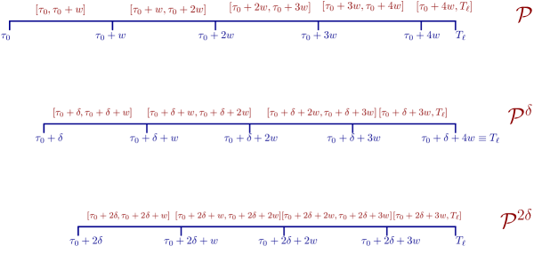
   Figure 1: Example of time windows selected for one patient.

   The collection of the time windows in $\mathcal{P}_{i}^{\textnormal{total}}$ (i.e., consecutive windows of 24 hours and their translations of 8 and 16 hours), allows to chunk the longitudinal evolution of the signals coherently with the way we extracted the low-frequency time-dependent covariates of Step 2. We shall refer to the portion of the vital signs signals corresponding to an interval in $\mathcal{P}_{i}^{\textnormal{total}}$ with the term time-series instance.

   

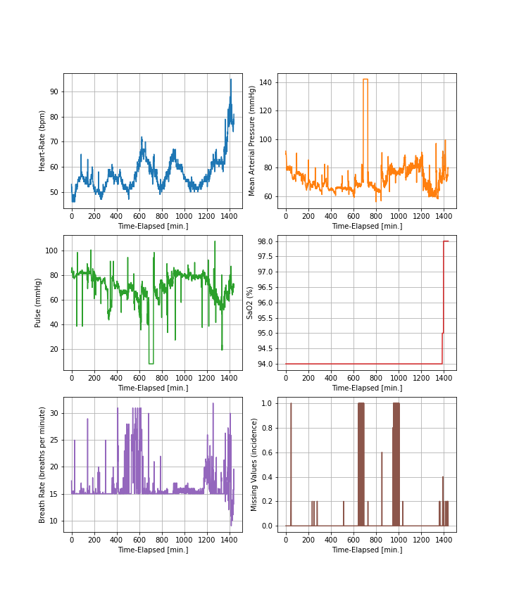
   Figure 2: Example of time-series instance. x-axis: time-domain (24 hours). y-axis: the values taken by each time-series feature. In specific, HR in blue, ABP in orange, pulse pressure in green, $\operatorname{SaO_{2}}$ in red, BR in purple, and the auxiliary time-series (with the missing values incidence) in brown.

3. Per each patient $i$ who has not acquired an infection during the stay in the ICU, we call not-infected instances all the instances whose time windows are in $\mathcal{P}_{i}^{\textnormal{total}}$.

4. For each patient $i$ who has acquired an infection during the stay in the ICU, we first divide the complete ICU as in point 2 ($\mathcal{P}_{i}^{\textnormal{total}}$). We then label all time-windows where an ICU-AI event has occurred as an outcome event (i.e., the time-window includes the time-stamp at which the ICU-AI episode has been recorded). In addition, we also label all the time windows preceding a time-window containing the onset of an ICU-AI event as outcome events. All remaining time windows are treated as non-infected.

5. We only consider the first ICU-AI and we discard all the other recurrent episodes from the same patient. Thus, all the instances following the first infection are discarded.

6. We equip each time-series instance with an extra time-series, monitoring the presence of missing values: in this way we can track the missing records at each time stamp.

Hence, each time-series instance can be described by a $6\times 1440$ matrix, whose rows represent the type of time-series features (i.e., HR, ABP, pulse pressure, SaO2, BR and missing records) and the columns the time domain. The illustration of one sample time-series instance is shown in Figure 2.

Missing values of vital signs signals have been imputed by using a zero-order spline, i.e., the Last Occurrence Carried Forward (LOCF) method. The inclusion of the missing values time-series helps the CNN to recognize the correct informativeness of flat patterns, i.e., whether a flat pattern is due to the LOCF method or not. We remark that our choice of 24-hour time window is only for the sake of illustrating the methodology. The analysis can be repeated with any window width (as done in Section 2 of the Supplementary material). However, the larger is the prediction window, the larger the dimensionality of the input data.

4.2 Design of the CNN

The CNN represents a specific class of Artificial Neural Networks (ANNs) which is designed to work with grid-structured data, e.g., time-series and images. Due to this intrinsic ability to process multi-level data, CNN have been widely applied in image recognition Liu, (2018); Zheng et al., (2017); Lou and Shi, (2020); Kagaya et al., (2014), anomaly detection Kwon et al., (2018); Naseer et al., (2018); Staar et al., (2019), and time-series forecasting Borovykh et al., (2017); Selvin et al., (2017); Livieris et al., (2020); Guo-yan et al., (2019). More specifically, convolutional and max-pooling operators are combined to encode the sequentiality of the patterns contained in the input data. As a result, the optimization of the weights of the convolutional filters of the convolutional layers aims to give the most linearized latent representation of the input time-series.

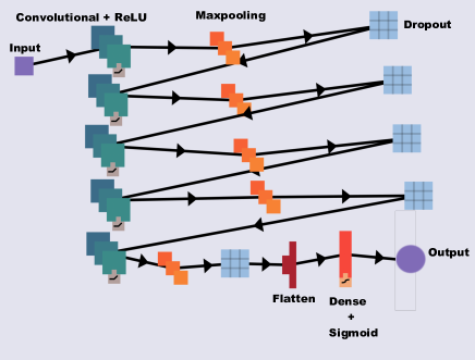
Figure 3: Schematic illustration of the CNN model. Starting from the left, the input signal is processed by a convolutional layer (128 filters of size 3). The a ReLU function is applied before a max-pooling operator that reduces the size of the features. After each max-pooling layer the network also contains a dropout layer whose dropout rate is 0.25. This sequence of hidden layers is repeated five times. The last feature map is flattened into an array and then propagated in a fully-connected layer (dense layer) with a sigmoid activation function.

In the present work we have chosen a pure convolutional network: its architecture is composed of convolutional, pooling, and dense layers only. The choice of a CNN seems natural, since we are looking for translational invariant patterns that might be present in any sub-interval in the time-series. However, in order to give quantitative grounds to this reasoning, in Section 2 of the Supplementary Material we compare CNN’s accuracy with other traditional NN-based models, namely Logistic Regression (LR), linear Supported Vector Machine (SVM), Multi Layer Perceptron (MLP), and CNN-LSTM networks (where LSTM stands for Long Short-Term Memory). We opted for a CNN design, due to its accuracy and to the possibility of applying the saliency maps analysis, presented in Section 6.

The final architecture chosen for the CNN is the following:

1. Convolutional Layers: the number of filters on each layer is 128, and each filter has a size of 3 (pixels). We call a feature map the output of a filter applied to the previous layer.

2. Activation Layer: the ReLU function (i.e. $\textnormal{ReLU}(x):=\max(0,x)$) is applied after each convolution operator. This application of a non-linear activation function on the feature maps gives rise to the activated feature maps.

3. Max-pooling layer: the activated feature maps are resampled via a max-pooling operator with a pooling size of 2 (sub-sampling).

The architecture also contains a dropout layer after each max-pooling layer. The dropout layer has a dropout rate of 0.25. This sequence of hidden layers is repeated five times. The last feature map is flattened into an array and then propagated into a fully-connected layer (dense layer) with a sigmoid activation function. The activation function returns a positive output between 0 and 1, that is, the risk score evaluated by the CNN. The architecture of the chosen CNN is sketched out in Figure 3. The figure is created by using the on-line tool ENNUI (https://math.mit.edu/ennui/).

4.3 Training and overall evaluation of the CNN

When training the model with the input EHR data, we used only a portion of the total amount of available EHR data. Indeed, we under-sampled the overall amount of EHR data to avoid both the training and the test set being too imbalanced. The number of time-series instances in the case group (i.e., those instances representing the ICU-AI episodes) are about one-twentieth of the total amount of time-series instances in the control group (i.e., those instances not representing the ICU-AI episodes). Thus, we fit the CNN model on a population of time-series instances with a control-case ratio of 8:1 (i.e., for each time-series instance in the case group one has eight time-series instances from the control group). It is important to stress that when under-sampling the EHR data, we apply a random under-sampling on the control group only. We use binary cross-entropy for the loss function, and the ADAM algorithm as the optimizer Kingma and Ba, (2015).

Since we train the CNN to solve a binary classification task, the Area Under the Receiver Operating Characteristic curve (AUROC) score Fawcett, (2006) represents the most appropriate choice for assessing the performance during the learning phase. Although we are not interested in the prediction formulated by the CNN in itself, we need to guarantee that the CNN model is able to classify the time-series instances and to encode informative patterns that describe the impending onset of an ICU-AI. Internal validation was performed using the K-folds cross-validation method. When validating the performance of CNN models as binary classifiers, the data were split into 5 folds. The overall AUROC is the average over the 5 folds. In Figure 3 of the Supplementary material the reader can find the behavior of the AUROC of the CNN model as function of three hyper-parameters of the network.

4.4 CNN Risk score

The extraction of the CNN score and its inclusion in the LM-CR model represent the novel ideas of the manuscript. The risk score of infection is evaluated by means of the CNN, whose architecture was discussed in Section 4.2 and its training in Section 4.3.

Thus, the procedure for evaluating the risk scores is the following:

1. Consider the vital signs signals of patient $i$ (HR, ABP, pulse pressure, SaO2, and RR) and the missing values time-series.

2. Starting from ICU admission time, extract 24-hour time-series instances by means of an 8-hour sliding time window (see Section 4.1), corresponding to the intervals in $\mathcal{P}_{i}$.

3. Propagate the time-series instances through the hidden layers of the fitted CNN model and evaluate the risk-score.

4. Assign the risk score to the corresponding time-stamp (i.e., day-month-hour-minute).

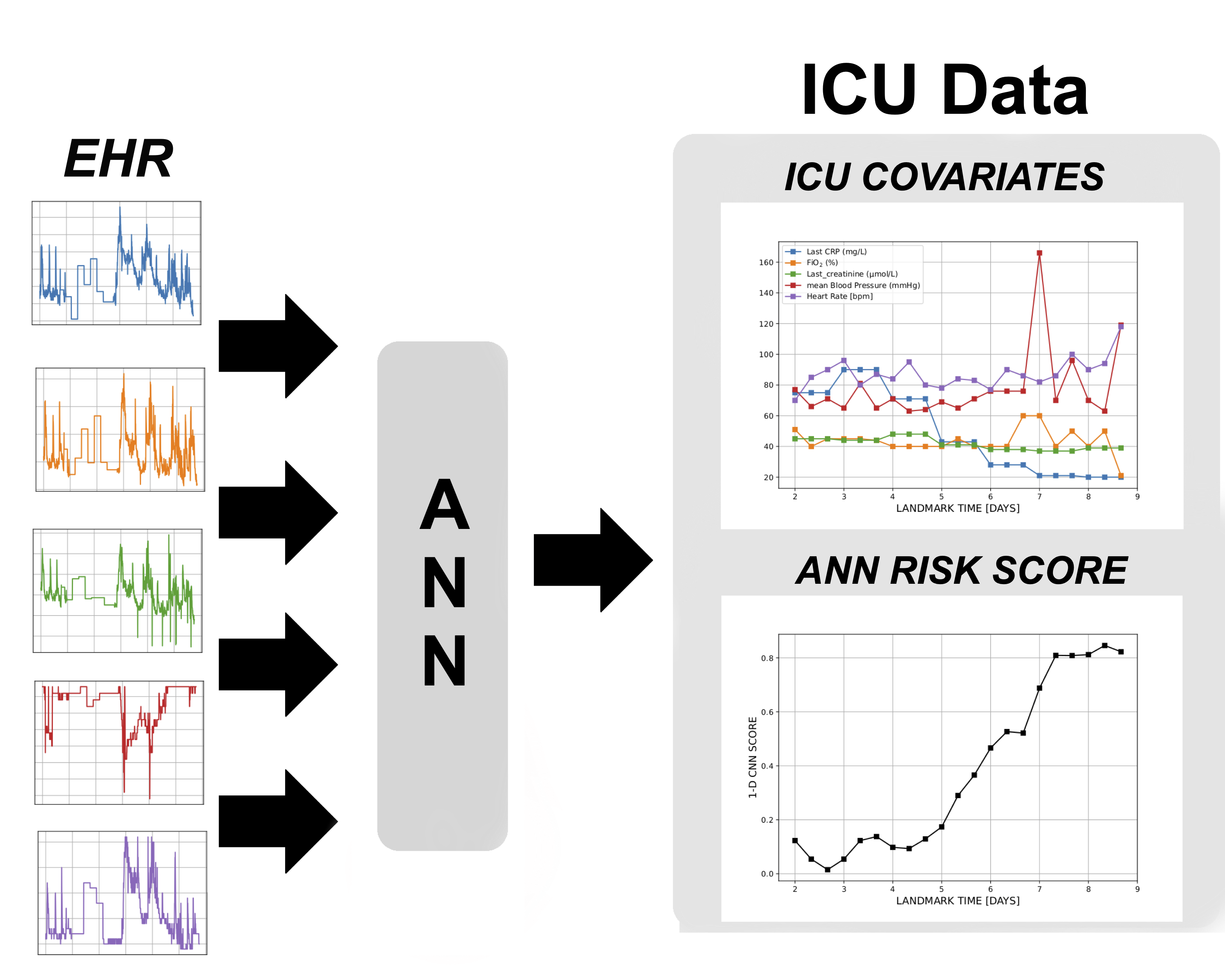
Figure 4: Schematic representation of the inclusion of the CNN-based risk score $Z_{\textnormal{CNN}}(t_{LM})$ in the ICU cohort data.

A scheme of how we incorporated the risk score into the ICU predictors is illustrated in Figure 4: for a single patient the score is calculated for each LM time $t_{LM}$. At each $t_{LM}$ the values of other time-dependent covariates are reported as well (e.g., CRP, $\textnormal{Fi}\textnormal{O}_{2}$, creatinine level, mean blood pressure, mean heart rate).

5 Step 2: Deep LM-CR model

5.1 Notations and LM-CR model

In this Section, we shall present the LM model following the notation used in Nicolaie et al., (2013).

We consider a cohort consisting of $N$ subjects, and we denote with $\tilde{T}$ the time of failure, $C$ the censoring time, $D$ the cause of failure, and $\mathbf{Z}(\cdot)$ and array of covariates. For the $i$-th subject, the tuple ($T_{i},\Delta_{i},\mathbf{Z}_{i}(\cdot)$) represents respectively the observed time $T_{i}=\min{(\tilde{T}_{i},C_{i})}$ (i.e., the earliest of failure and censoring time), the cause of failure $\Delta_{i}=\mathbf{1}(\tilde{T}_{i}<C_{i})D_{i}$ (with $\mathbf{1}(\cdot)$ the indicator function), and $\mathbf{Z}_{i}(\cdot)$ the covariates up to time $T_{i}$. Likewise, we shall adopt the subscript $j$ to refer to the competing causes of failure, with $j\in\{1,\dots,J\}$.

We would like to derive a dynamic prediction of the probability distribution function of the failure time of cause $j$ at some time horizon ($t_{hor}$), conditional on surviving event free and on the information available at a fixed time $t_{LM}$ (landmark time). More specifically, given a prediction window $w$ (such that $t_{hor}=t_{LM}+w$) we would like to estimate the survival probability and the Cumulative Incidence Function (CIF) of cause $j$:

$$S_{LM}(t_{hor}|\mathbf{Z}(t_{LM}),t_{LM}):=\mathbb{P}(T>t_{hor}|\mathbf{Z}(t_{LM}),t_{LM}),$$ (1)

$$F_{j,LM}(t_{hor}|\mathbf{Z}(t_{LM}),t_{LM}):=\mathbb{P}(T\leq t_{hor},\Delta=j|\mathbf{Z}(t_{LM}),t_{LM}).$$ (2)

The LM approach consists of two steps:

1. We first divide the time domain of our observations $[s_{0},s_{1}]$ into $n$ equi-spaced landmark points denoted with $\{t_{LM}^{k}\}_{k=1}^{n}$, where $t_{LM}^{1}\equiv s_{0}$ and $t_{LM}^{n}\equiv s_{1}$. Hence, we fix the width of the prediction window $w$ (i.e., the lead time), and then for each LM time $t_{LM}^{k}$ we create a dataset by selecting all the subjects at risk at time $t_{LM}^{k}$ and by imposing administrative right-censoring at the time $t_{LM}^{k}+w$ (horizon time). Thus, for a vector of time-dependent covariates $\mathbf{Z}(t)$, only the values $\mathbf{Z}(t_{LM}^{k})$ at $t_{LM}^{k}$ are considered in the $k$-th dataset. Finally, we create an extensive dataset by stacking all the datasets extracted at each landmark time $t_{LM}^{k}$ (LM super-dateset).

2. The second step is fitting the LM-CR super-model on the stacked LM super-dateset Nicolaie et al., (2013). Since at each $t_{LM}^{k}$, the vector $\mathbf{Z}(t_{LM}^{k})$ is treated as a time constant vector of covariates, the dataset can be analyzed by using standard survival analysis methods.

In the LM-CR super-model we fit indeed a Cox proportional hazard model for the cause specific hazard $\lambda_{j}$:

$$\lambda_{j}(t|t_{LM},\mathbf{Z}(t_{LM}))=\lambda_{0j}(t|t_{LM})\exp{[\beta^{T}_{j}(t_{LM})\mathbf{Z}(t_{LM})]},$$ (3)

where $\lambda_{0j}(t|t_{LM})$ denotes the (unspecified) baseline hazards and $\beta_{j}(t_{LM})$ the set of regressors specific for the $j$-th cause in within the interval interval $[t_{LM},t_{LM}+w]$. We assume that the coefficients $\beta$ depend on $t_{LM}$ in a smooth way, i.e., $\beta_{j}(t_{LM})=f_{j}(t_{LM},{\beta}^{(0)}_{j})$ with ${\beta}_{j}^{(0)}$ a vector of regression parameter and $f_{\beta}(\cdot)$ a parametric function on time, e.g., a spline. Our choice has been a quadratic function:

$$\beta_{j}(t_{LM}):={\beta}_{j}^{(0)}+\beta_{j}^{(1)}t_{LM}+\beta_{j}^{(2)}t_{LM}^{2}$$

Fitting this model with the Breslow partial likelihood for tied observations is equivalent to maximizing the pseudo-partial log-likelihood as shown in Nicolaie et al., (2013). The landmark supermodel can be then fitted directly by applying a simple Cox model to the stacked data set. Hence, after having estimated the coefficients and the baseline cause specific hazards, we get the plug-in estimators for the survival probabilities (i.e., $\hat{S}_{LM}(t_{hor}|\boldsymbol{Z}(t_{LM}),t_{LM})$) and of the CIF of cause $j$ (i.e., $\hat{F}_{j,LM}(t_{hor}|\boldsymbol{Z}(t_{LM}),t_{LM})$).

5.2 LM-CR for ICU-AI

In the context of dynamic predictions for ICU-AIs, we adopted a CR model with three causes of failure: ICU-AI, death in the ICU and discharge; see Figure 5. No right censoring is present in the data, since no patient left the ICU before discharge or death.

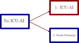
Figure 5: Competing risks model for ICU-AI.

Following the notation used in Section 5.1, we denote with $\tilde{T}$ the time of failure, $D$ the cause of failure (i.e., $D=1$ denotes an ICU-AI, while $D=2$ discharge or death), and $\mathbf{Z}(\cdot)$ the array of covariates. For the $i$-th subject the triple ($T_{i},\Delta_{i},\mathbf{Z}_{i}(\cdot)$) denotes the observed time $T_{i}\equiv\tilde{T}_{i}$, the cause of failure $\Delta_{i}\equiv D_{i}$, and $\mathbf{Z}_{i}(\cdot)$ the vector of covariates.

In this article, we consider the prediction window was set to $w=24$ hours. The time domain is $[s_{0},s_{1}]$, with $s_{0}=48$ hours and $s_{1}=240$ hours, and we consider $n=25$ LM times $t_{LM}$, i.e., two subsequent LM times are at distance 8 hrs.

If we denote with $Z_{\textnormal{CNN}}(t)$ the CNN risk score at time $t$ (see Figure 4) and with $\mathbf{Z}(t)$ the vector of all the other covariates in the LM-CR model at time $t$, we are interested at the dynamic predictions of the two models:

1. $\pi_{1}:={F}_{1,LM}(t_{hor}|\mathbf{Z}(t_{LM}),t_{LM})$: i.e., the CIF of infection conditioned on the survival up to time $t_{LM}$ and on the low frequency covariates (LM-CR model);

2. $\pi_{2}:={F}_{1,LM}(t_{hor}|\mathbf{Z}(t_{LM}),Z_{\textnormal{CNN}}(t_{LM}),t_{LM})$: the CIF of infection conditioned on the survival up to time $t_{LM}$ and on both the low frequency covariates and $Z_{\textnormal{CNN}}$ (Deep-LM-CR model).

By comparing the accuracies of $\pi_{1}$ and $\pi_{2}$, we can measure the added predictive power of the CNN score. We shall refer at the first model with LM-CR and to the second with Deep-LM-CR.

5.3 Evaluation of LM-CR model

We use the AUROC metric to evaluate the prediction made at each single landmark time. When considering an overall measure, the evaluation of a global AUROC needs to consider the time-dependent character of the dynamic. Similarly to the estimator of the prediction error proposed in Spitoni et al., (2018), the evaluation of the overall AUROC needs to take into account the change in time of the size of the risk-set. The absence of censoring allows us to estimate the overall AUROC score simply by:

$$\operatorname{AUROC_{global}}=\frac{\sum_{k=1}^{n}R(t_{LM}^{k})\operatorname{AUROC}(t_{LM}^{k})}{\sum_{k=1}^{n}R(t_{LM}^{k})},$$ (4)

with $t_{LM}^{k}$ the $k$-th landmark time, $n$ the total number of landmark times, and $R(t_{LM}^{k})$ the size of the risk-set at time $t_{LM}^{k}$.

The influence of the individual predictor in the prediction has been visualized by means of heat-maps. We compute the relative variation of the overall AUROC between the model including all predictors and the one where the predictor is removed. Thus, we construct a heat-map representing the relative change in AUROC due the removal of a single predictor at landmarking time $t_{LM}$.

Finally, we remark that internal validation was performed using a 10-folds cross-validation method. The overall $\operatorname{AUROC_{global}}$ and the $\operatorname{AUROC}(t_{LM}^{k})$, evaluated at each time $t_{LM}^{k}$, are averaged over the 10 folds. In both the CR-LM model and the Deep-CR-LM model, we report 95% bootstrap confidence intervals.

5.4 Results

In this Section we are going to show that the CNN risk score $Z_{\textnormal{CNN}}$ adds extra predictive information to the model, not present in the standard covariates.

In Figure 6 we plotted the empirical distribution of $Z_{\textnormal{CNN}}(t_{LM})$ for three landmark points (i.e., $t_{LM}\in\{3,6,8\}$) and stratified by the cause of failure. As expected, the distribution of $Z_{\textnormal{CNN}}$ for infected patients is more skewed on the right: while at day three this phenomenon is mild, at days 6 and 8 the skewness of the density distribution is much more evident.

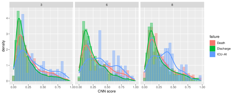
Figure 6: Distribution of the CNN risk score at three different landmark points ($t_{LM}^{k}\in\{3,6,8\}$ days), stratified for the cause of failure.

In Figure 7 we report the Pearson correlations between the CNN risk score and the vital signals averaged in the 24hrs time windows prior the landmark (time-dependent covariates included in the LM-CR). Although the risk score is evaluated relative to these signals, only mild correlations are present. Our main hypothesis is indeed that $Z_{CNN}(t_{LM})$ has added predictive information, not contained in the other covariates $\mathbf{Z}(t_{LM})$.

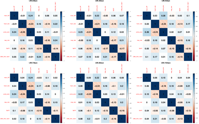
Figure 7: Correlation plot: CNN risk score vs. the vital signals (averaged in the 24 hours before the landmark).

Moreover, with regards to the cause specific hazards for infection, the CNN risk score turned out to be the most important predictor: $\beta^{(0)}_{1;\textnormal{CNN}}=4.8$ (95%CI 3.05-6.72). All the cause-specific hazards for ICU-AI are reported in Table 3 of the Supplementary Material.

The LM approach provides a plug-in estimator for the dynamic prediction (2) of the CIFs of ICU-AI. Therefore, in order to give an example of the dynamic prediction allowed by the model, in Figure 8 we report the CIFs for the LM-CR and the Deep-LM-CR models as function of the landmark time and of the quantile groups of the fitted linear predictors. Given the value of the covariates at the landmark time $t_{LM}$, the CIF at any $s$, with $s\in[t_{TM},t_{LM}+w]$ is given indeed by the plug-in estimator $\hat{F}_{1,LM}(s|\boldsymbol{Z}(t_{LM}),t_{LM})$ of (2). The dashed red line in Figure 8 denotes an arbitrary warning level for the CIF of infection (e.g., $8\%$). We can see that, for the forth quantile $Q_{4}$ and at LM time $t_{LM}=4$ days, the Deep-LM-CR model has a lead time of circa 3 hours in reaching the warning threshold before the LM-CR model.

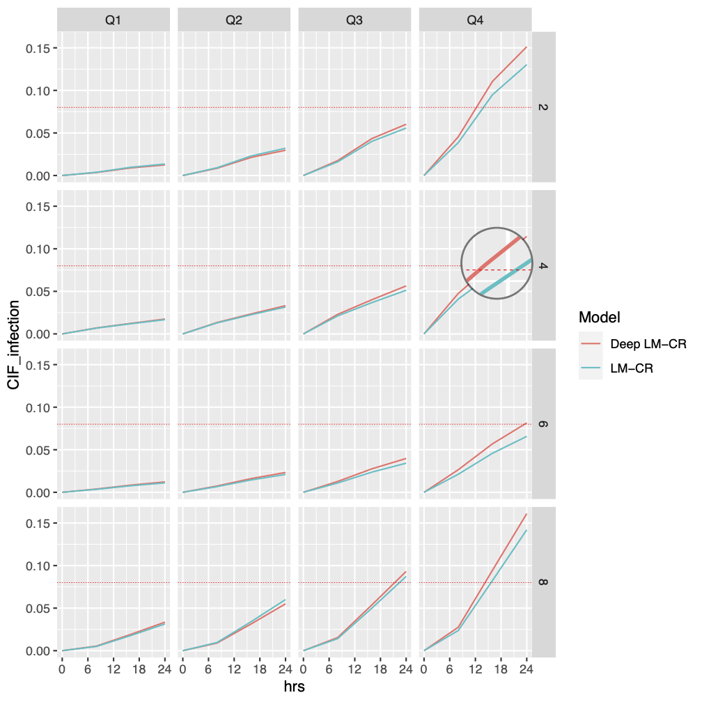
Figure 8: Comparison of the CIFs at different landmark time (i.e., $t_{LM}^{k}\in\{2,4,6,8\}$ days) of the models LM-CR and Deep-LM-CR.

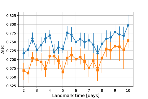
Figure 9: AUROC score (y-axis) as a function of the landmark times (x-axis). The two curves represent the predictive performance of the basic CR-LM model (orange), and of the Deep-CR-LM model (blue) The error bars denote the 95% bootstrap confidence intervals.

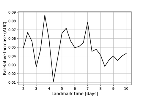
Figure 10: ICU-AI: overall relative increase of AUROC score (y-axis) as a function of the landmark times (x-axis) when including CNN-based risk score.

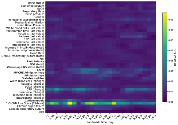
Figure 11: AUC heat-maps evaluating the impact of each predictor in the Deep-LM-CR model when predicting ICU-AI. The color of each pixel denotes the magnitude of the impact (relative AUROC increase) of one covariate (y-axis) with respect to the LM time (x-axis).

The overall measure for the LM-CR model is $\operatorname{AUROC_{global}}=0.69$ (95%CI 0.68-0.70), while for the Deep-LM-CR is $\operatorname{AUROC_{global}}=0.75$ (95%CI 0.73-0.76). The $\operatorname{AUROC}(t_{LM}^{k})$ scores evaluated at each time $t_{LM}^{k}$, with $k\in\{1,\ldots,n\}$ are shown in Figure 9. The LM-CR model always shows lower predictive performance than the Deep-LM-CR. We notice that at the beginning of the ICU stay (days 3-4) and around day 7, the CNN can improve the prediction of the traditional ICU clinical covariates of about $8\%$, see Figure 10.

The impact of each explanatory variable $Z_{j}$ involved in the Deep-LM-CR model is shown in Figure 11, whereas we reported the heat-map of the relative increase in AUROC between the Deep-LM-CR without the covariate $Z_{j}$ and the full model (with $\mathbf{Z}(t_{LM})$ and $Z_{CNN}(t_{LM}))$. When $Z_{j}=Z_{CNN}$, we see that we observe a relative increase in AUROC of at least $4\%$.

Summing up, we have shown that the two-step modeling can effectively lead to an increase of the accuracy of the predictions. The extra predicting power comes from the inclusion of the CNN-based risk score, which is a summary measure of the predicting patterns found by the CNN model trained on only five vital signs signals (sample frequency of 1 minute).

We remark that in our analysis we did not consider recurrent infections, but we limited the attention to the first episode of ICU-AI.

6 Explainability of CNN-based prediction of ICU-AI

In this section, we present an attempt to make interpretable the activity of the CNN. As shown in Section 5.4, the CNN-based risk score has added predicting power to the LM-CR model. However, for the moment, we do not have any information about the saliency of the vital signs signals selected by the CNN during the training. This knowledge might be crucial for shedding some light on the relation between the activity of pattern recognition of the network and the medical conditions of a patient when a ICU-AI is approaching.

To investigate which characteristics of the pattern selected by the CNN, we use the so-called Explainable Artificial Intelligence (XAI), namely a class of methods designed to understand the decisions and the predictions formulated by ANN techniques Phillips et al., (2020); Vilone and Longo, (2021); Castelvecchi, (2016). The scope of XAI is to contrast indeed the widespread black box attitude that many users have when applying ANN techniques.

6.1 Explanability via SMOE scale

A saliency map is a map acting on the activated features in the hidden layers, generally used for showing which parts of the input are most important for the network’s decisions. The Saliency Map Order Equivalent scale (SMOE) used in the present paper is base on the algorithm developed by Mundhenk et al., (2019): an efficient and non-gradient method based on the statistical analysis of the activated feature maps. For a more detailed description of the SMOE scale, we refer the reader to Section 3 of the Supplementary Material.

We would like to use the saliency maps for selecting, in the original 24hrs time-series, the most relevant 8-hours patterns.

The adopted approach is the following:

1. We fit three different CNNs, one for each of $t_{LM}^{k}\in\{3,7,10\}$. We consider three distinct CNNs because the predicting patterns found by the network might differ among different periods of the ICU stay (see for instance the discussion in Section 6.3). The LM point 3 days is a proxy for an early time of the stay, 7 days for an intermediate time, and finally 10 days for a later moment. The design of the networks is the same as described in Section 4.2. All these models are validated via 5-fold cross-validation.

2. We study the pattern recognition performed by the hidden layer, and we make it interpretable via the SMOE scale. Through this method, we can visualize the regions of the input data with the highest saliency. Specifically, for each model developed at every LM time $t_{LM}^{k}$, we construct and visualize the saliency maps of the test set only. We repeat this action for each test set of each cross-validation fold.

3. From each saliency map, we extract the 8-hours interval with the highest cumulative saliency value. After having extracted the most relevant 8-hour patterns from each time-series instance, we can focus on their interpretation and their clustering. An example of the extraction of the 8-hours most salient pattern is shown in Figure 12.

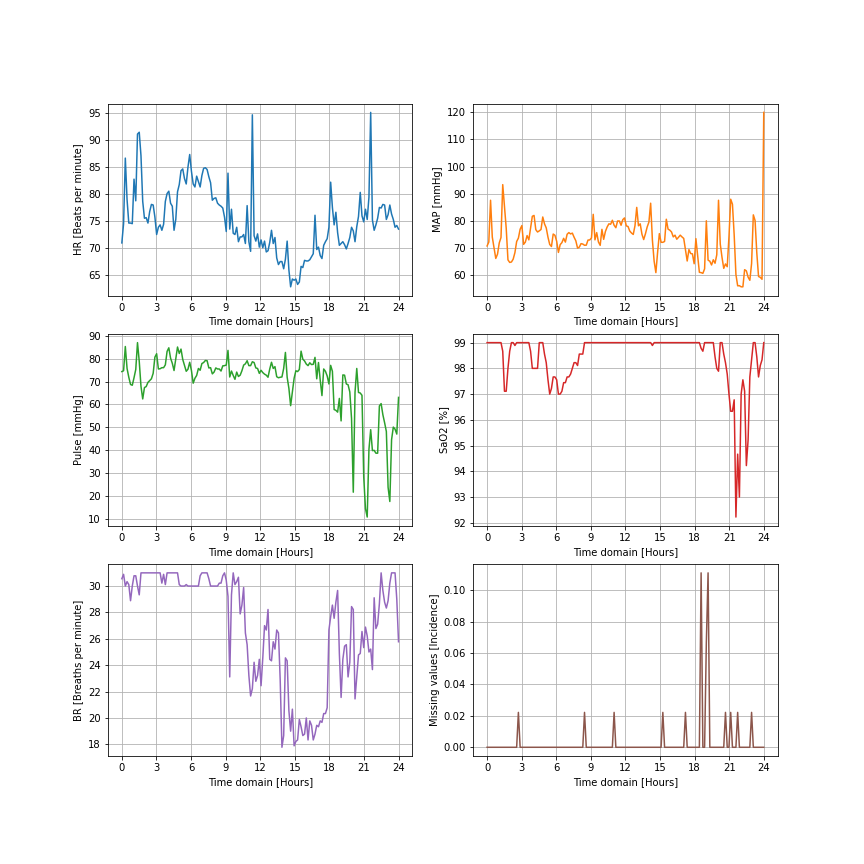
(a)

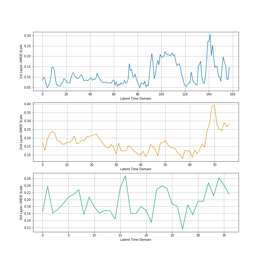
(b)

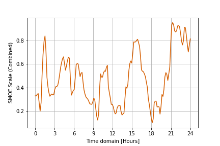
(c)

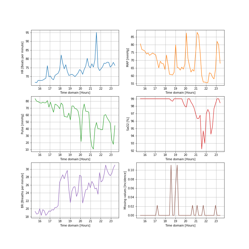
(d)

Figure 12: Schematic example of the extraction of the most salient patterns in the 24-hours time-series instances: (a) Example of time-series instance, (b) SMOE scale applied on each activation feature map of the CNN, (c) Averaged saliency map (weighted average of SMOE scales on individual hidden layers), (d) extraction of the most salient interval of (a).

6.2 Data-driven clustering of salient patterns

We focus now the attention on the clustering of the most salient patters extracted in Section 6.1. We would like indeed to answer the question: how can we link the activity of pattern recognition to some medical conditions, appearing when a ICU-AI is approaching? Our strategy for answering the question is the following:

1. We collect the set of the most predictive patterns with amplitude 8 hours, obtained by applying the SMOE scale to the time-series instances, as explained in Section 6.1.

2. We consider four clinical critical conditions, i.e., tachycardia, hypotension, desaturation, and hyperventilation (see Table 1), which could predict the approaching of one ICU-AI episode. These medical conditions reflect the main symptoms of the Systemic Inflammatory Response Syndrome (SIRS), see Chakraborty and Burns, (2019). Tachycardia, hypotension, and hyperventilation are quite spread in the ICU, and they usually mentioned in general guidelines for the ascertainment of SIRS Comstedt et al., (2009). For the criteria reported in Table 1 we refer to Comstedt et al., (2009); in specific for Desaturation, we refer to Hafen and Sharma, (2022).

3. We evaluate the mean values of HR, ABP, $\operatorname{SaO_{2}}$ and BR for each of the most salient 8-hour pattern extracted via the SMOE scale. Depending on the values obtained (see the criteria in Table 1), we check the presence of the four clinical critical conditions. Thus, the combination of these conditions produces 16 different possible clinical situations of interest, as shown in Table 2: they represent the classes of the proposed data-driven clustering. In Figure 13 the 16 distinct classes are represented as nodes of a graph (i.e., a four dimensional hypercube).

Critical Condition	Criterion
Tachycardia	Hearth Rate $\geq$90 beats per minute
Hypotension	Arterial Blood Pressure (mean) $\leq$ 80mmHg
Desaturation	$\operatorname{SaO_{2}}\leq$ 95%
Hyperventilation	Breath Rate $\geq$ 24 breaths per minute

Table 1: Critical conditions and their criteria.

Class	Data Driven Cluster (Clinical Conditions)
0	None
1	Tachycardia
2	Hypotension
3	Hypotension, Tachycardia
4	Desaturation
5	Desaturation, Tachycardia
6	Desaturation, Hypotension
7	Desaturation, Hypotension, Tachycardia
8	Hyperventilation
9	Hyperventilation, Tachycardia
10	Hyperventilation, Hypotension
11	Hyperventilation, Hypotension, Tachycardia
12	Hyperventilation, Desaturation
13	Hyperventilation, Desaturation, Tachycardia
14	Hyperventilation, Desaturation, Hypotension
15	Hyperventilation, Desaturation, Hypotension, Tachycardia

Table 2: List of the 16 clinical conditions (classes of the clustering).

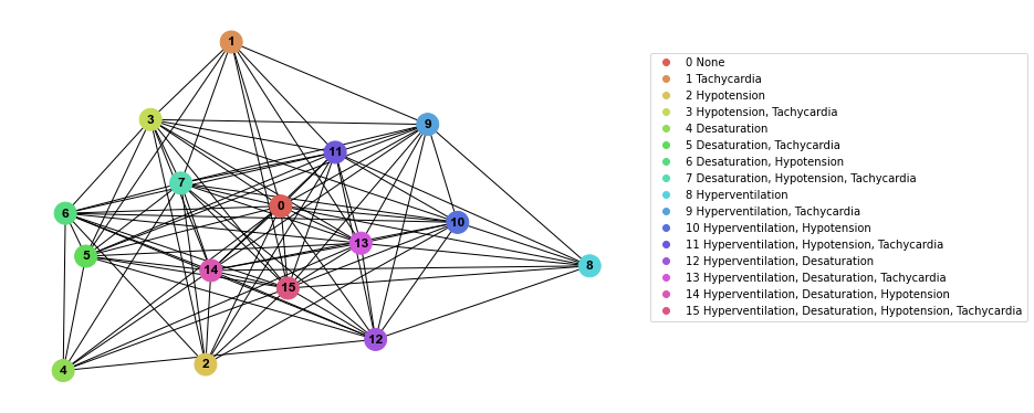
Figure 13: Graph whose nodes represent the 16 classes of the clustering.

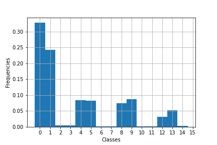
(a)

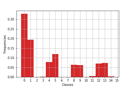
(b)

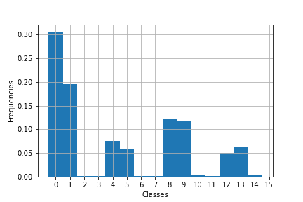
(c)

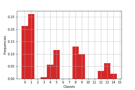
(d)

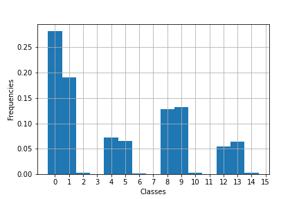
(e)

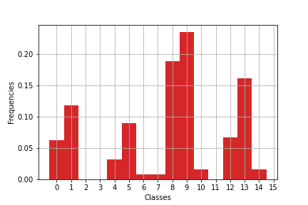
(f)

Figure 14: Histograms the data-driven clustering approach. Bins on the x-axis represent the 16 classes. Blue histograms concern the non-infected instances, whereas the red ones the infected instances. CNN trained on day 3 is described by (a) and (b), on day 7 by (c) and (d), and on day 10 by (e) and (f).

6.3 Results of the data-driven clustering

Histograms with the relative frequencies of the 16 data-driven clusters are shown in Figure 14. For day 3 (see Figures 14(a) and 14(b)), a two-sample Kolmogorov-Smirnov test Hodges, (1958) reveals that the sample distributions of the classes between not-infected and infected instances are not significantly different (p-value=0.21). However, we can observe a completely different scenario on both days 7 and 10 (see Figure 14 (d)-(f)), where the null hypothesis of the two-samples Kolmorogov-Smirnov test is rejected (p-value= 0.0003 and p-value= $10^{-10}$ respectively). Hence, this analysis shows that different clinical conditions could represent an essential feature of the patterns that the CNN model captures during the learning phase. For instance, for infected instances, at day 10, the prevalence of at least one of these 16 conditions is around 94%, while 79% at day 7; see Figure 14 (d)-(f)). Precisely, on day 10, events with hyperventilation correspond at 70% of samples, and in combination with tachycardia 23%. While a day 7 tachycardia is much more relevant and occurs in 50% of infectious samples. Therefore, the most salient 8-hours subinterval of our time-series instance can be linked to precise medical conditions, which are known to be related to the presence of an ICU-AI.

7 Conclusions

We have showed that the proposed two-step modeling of ICU-AI is at the same time an accurate predicting tool and an interpretable model. The CNN is able to detect predicting patterns by analyzing the time-series of five vital sign signals. These patters contain extra predictive information and they are only mildly correlated with the averaged quantities of the vital signals, routinely included in the traditional survival models. Moreover, we have showed as well that the SMOE scale might help physicians in clustering patients with an approaching infection.

We have illustrated the methodology in a competing risks framework. However, recently the LM approach has been extended to multi-state models, even without the Markov assumption Putter and Spitoni, (2018); Hoff et al., (2019). Therefore, as a further extension we could model recurrent infections as new states in a non-Markov multi state model, with transition hazards that might depend indeed on the previous infections’ sequence. Moreover, another future challenging direction of investigation is a sort of inversion of the CNN, in order to identify and classify the patterns in the signal with higher predicting power. This analysis might help in performing a more precise clustering of the patients with fore-coming ICU-AI.

Code Availability

Python codes and modules are available on GitHub: the reader can refer to https://github.com/glancia93/ICUAI-dynamic-prediction/blob/main/ICUAI_module.py.

References

- Andersen et al., (1993) Andersen, P. K., Borgan, O., Gill, R. D., and Keiding, N. (1993). Statistical Models Based on Counting Processes. Springer.
- Borovykh et al., (2017) Borovykh, A., Bohte, S., and Oosterlee, K. (2017). Conditional time series forecasting with convolutional neural networks. In Lecture Notes in Computer Science/Lecture Notes in Artificial Intelligence, pages 729–730.
- Castelvecchi, (2016) Castelvecchi, D. (2016). Can we open the black box of ai? Nature News, 538(7623):20.
- Chakraborty and Burns, (2019) Chakraborty, R. K. and Burns, B. (2019). Systemic inflammatory response syndrome.
- Comstedt et al., (2009) Comstedt, P., Storgaard, M., and Lassen, A. T. (2009). The systemic inflammatory response syndrome (sirs) in acutely hospitalised medical patients: a cohort study. Scandinavian journal of trauma, resuscitation and emergency medicine, 17(1):1–6.
- Cortese and Andersen, (2010) Cortese, G. and Andersen, P. K. (2010). Competing risks and time-dependent covariates. Biometrical Journal, 52(1):138–158.
- Dantes and Epstein, (2018) Dantes, R. B. and Epstein, L. (2018). Combatting sepsis: a public health perspective. Clinical infectious diseases, 67(8):1300–1302.
- Fawcett, (2006) Fawcett, T. (2006). An introduction to roc analysis. Pattern Recognition Letters, 27(8):861–874. ROC Analysis in Pattern Recognition.
- Ferrer et al., (2019) Ferrer, L., Putter, H., and Proust-Lima, C. (2019). Individual dynamic predictions using landmarking and joint modeling: Validation of estimators and robustness assessment. Statistical Methods in Medical Research, 28(12):3649–3666.
- Guo-yan et al., (2019) Guo-yan, X., Jin, Z., Cun-you, S., Wen-bin, H., and Fan, L. (2019). Combined hydrological time series forecasting model based on cnn and mc. Computer and Modernization, (11):23.
- Hafen and Sharma, (2022) Hafen, B. B. and Sharma, S. (2022). Oxygen saturation. StatPearls, StatPearls Publishing.
- Hodges, (1958) Hodges, J. L. (1958). The significance probability of the smirnov two-sample test. Arkiv för Matematik, 3(5):469–486.
- Hoff et al., (2019) Hoff, R., Putter, H., Mehlum, I. S., and Gran, J. M. (2019). Landmark estimation of transition probabilities in non-markov multi-state models with covariates. Lifetime Data Analysis, 25(4):660–680.
- Ivanov et al., (2022) Ivanov, O., Molander, K., Dunne, R., Liu, S., Masek, K., Lewis, E., Wolf, L., Travers, D., Brecher, D., Delaney, D., et al. (2022). Accurate detection of sepsis at ed triage using machine learning with clinical natural language processing. arXiv preprint arXiv:2204.07657.
- Kagaya et al., (2014) Kagaya, H., Aizawa, K., and Ogawa, M. (2014). Food detection and recognition using convolutional neural network. In Proceedings of the 22nd ACM international conference on Multimedia, pages 1085–1088.
- Kingma and Ba, (2015) Kingma, D. P. and Ba, J. (2015). Adam: A method for stochastic optimization. In ICLR.
- Klouwenberg et al., (2013) Klouwenberg, P. M. K., Ong, D. S., Bos, L. D., de Beer, F. M., van Hooijdonk, R. T., Huson, M. A., Straat, M., van Vught, L. A., Wieske, L., Horn, J., et al. (2013). Interobserver agreement of centers for disease control and prevention criteria for classifying infections in critically ill patients. Critical care medicine, 41(10):2373–2378.
- Kwon et al., (2018) Kwon, D., Natarajan, K., Suh, S. C., Kim, H., and Kim, J. (2018). An empirical study on network anomaly detection using convolutional neural networks. In ICDCS, pages 1595–1598.
- Liu, (2018) Liu, Y. H. (2018). Feature extraction and image recognition with convolutional neural networks. In Journal of Physics: Conference Series, volume 1087, page 062032. IOP Publishing.
- Livieris et al., (2020) Livieris, I. E., Pintelas, E., and Pintelas, P. (2020). A cnn–lstm model for gold price time-series forecasting. Neural computing and applications, 32(23):17351–17360.
- Lou and Shi, (2020) Lou, G. and Shi, H. (2020). Face image recognition based on convolutional neural network. China Communications, 17(2):117–124.
- Maki et al., (2008) Maki, D. G., Crnich, C. J., and Safdar, N. (2008). Nosocomial infection in the intensive care unit. Critical care medicine, page 1003.
- May et al., (2011) May, R., Dandy, G., and Maier, H. (2011). Review of input variable selection methods for artificial neural networks. In Suzuki, K., editor, Artificial Neural Networks, chapter 2. IntechOpen, Rijeka.
- Mundhenk et al., (2019) Mundhenk, T. N., Chen, B. Y., and Friedland, G. (2019). Efficient saliency maps for explainable ai. arXiv preprint arXiv:1911.11293.
- Naseer et al., (2018) Naseer, S., Saleem, Y., Khalid, S., Bashir, M. K., Han, J., Iqbal, M. M., and Han, K. (2018). Enhanced network anomaly detection based on deep neural networks. IEEE access, 6:48231–48246.
- Nicolaie et al., (2013) Nicolaie, M., Van Houwelingen, J., De Witte, T., and Putter, H. (2013). Dynamic prediction by landmarking in competing risks. Statistics in medicine, 32(12):2031–2047.
- Phillips et al., (2020) Phillips, P. J., Hahn, C. A., Fontana, P. C., Broniatowski, D. A., and Przybocki, M. A. (2020). Four principles of explainable artificial intelligence. Gaithersburg, Maryland.
- Proust-Lima and Taylor, (2009) Proust-Lima, C. and Taylor, J. M. (2009). Development and validation of a dynamic prognostic tool for prostate cancer recurrence using repeated measures of posttreatment psa: a joint modeling approach. Biostatistics, 10(3):535–549.
- Putter and Spitoni, (2018) Putter, H. and Spitoni, C. (2018). Non-parametric estimation of transition probabilities in non-markov multi-state models: The landmark aalen–johansen estimator. Statistical Methods in Medical Research, 27(7):2081–2092.
- Rizopoulos, (2011) Rizopoulos, D. (2011). Dynamic predictions and prospective accuracy in joint models for longitudinal and time-to-event data. Biometrics, 67(3):819–829.
- Rizopoulos, (2012) Rizopoulos, D. (2012). Joint models for longitudinal and time-to-event data: With applications in R. CRC press.
- Selvin et al., (2017) Selvin, S., Vinayakumar, R., Gopalakrishnan, E., Menon, V. K., and Soman, K. (2017). Stock price prediction using lstm, rnn and cnn-sliding window model. In 2017 international conference on advances in computing, communications and informatics (icacci), pages 1643–1647. IEEE.
- Spitoni et al., (2018) Spitoni, C., Lammens, V., and Putter, H. (2018). Prediction errors for state occupation and transition probabilities in multi-state models. Biometrical Journal, 60(1):34–48.
- Staar et al., (2019) Staar, B., Lütjen, M., and Freitag, M. (2019). Anomaly detection with convolutional neural networks for industrial surface inspection. Procedia CIRP, 79:484–489.
- Topol, (2019) Topol, E. J. (2019). High-performance medicine: the convergence of human and artificial intelligence. Nature medicine, 25(1):44–56.
- van Houwelingen and Putter, (2011) van Houwelingen, H. and Putter, H. (2011). Dynamic prediction in clinical survival analysis. CRC Press.
- Van Houwelingen, (2007) Van Houwelingen, H. C. (2007). Dynamic prediction by landmarking in event history analysis. Scandinavian Journal of Statistics, 34(1):70–85.
- Vilone and Longo, (2021) Vilone, G. and Longo, L. (2021). Notions of explainability and evaluation approaches for explainable artificial intelligence. Information Fusion, 76:89–106.
- Vincent et al., (2009) Vincent, J., Rello, J., and Marshall, J. (2009). International study of the prevalence and outcomes of infection in intensive care units. JAMA, 302(21):2323–9.
- Zeng et al., (2022) Zeng, Z., Hou, Z., Li, T., Deng, L., Hou, J., Huang, X., Li, J., Sun, M., Wang, Y., Wu, Q., et al. (2022). A deep learning approach to predicting ventilator parameters for mechanically ventilated septic patients. arXiv preprint arXiv:2202.10921.
- Zheng et al., (2017) Zheng, H., Fu, J., Mei, T., and Luo, J. (2017). Learning multi-attention convolutional neural network for fine-grained image recognition. In Proceedings of the IEEE international conference on computer vision, pages 5209–5217.