Modelling sample-to-sample fluctuations of the gap ratio in finite disordered spin chains
Abstract
We study sample-to-sample fluctuations of the gap ratio in the energy spectra in finite disordered spin chains. The chains are described by the random-field Ising model and the Heisenberg model. We show that away from the ergodic/nonergodic crossover, the fluctuations are correctly captured by the Rosenzweig-Porter (RP) model. However, fluctuations in the microscopic models significantly exceed those in the RP model in the vicinity of the crossover. We show that upon introducing an extension to the RP model, one correctly reproduces the fluctuations in all regimes, i.e., in the ergodic and nonergodic regimes as well as at the crossover between them. Finally, we demonstrate how to reduce the sample-to-sample fluctuations in both studied microscopic models.
I Introduction
Switching on interactions in low–dimensional Anderson insulators leads through the interplay between the quantum interference and many–body interactions to fascinating new phenomena. While turning on interactions at small disorder delocalizes the system, the strong disorder is believed to cause many–body (MBL) localization [1, 2, 3, 4] at least on finite–size lattices. Even though research in this field predominantly focused on a few simplest prototype model Hamiltonians for MBL, such as the disordered XXZ model [5, 6, 7, 8, 9, 10, 11, 12, 13, 14, 15, 16], the type of the transition and even the existence of the MBL phase in the thermodynamic limit are still under intense consideration [17, 18, 19, 20, 21, 22, 23, 24, 25, 26, 27, 28]. The latest results based on the studies of the avalanche instability suggest that the transition to the MBL phase occurs for much stronger disorder then it follows from the previous numerical studies of finite systems [26].
At small disorder, the quantum many-body system is ergodic; its energy spectrum can be analyzed within the framework of the random matrix theory (RMT), while the eigenstate thermalization hypothesis can describe the relaxation of physical observables of a closed system [29, 30, 31, 32, 33, 34, 32, 35, 36, 37, 38, 39, 40, 41, 42, 43, 44, 45, 46]. Increasing the disorder strength leads to the ergodicity breakdown that is reflected in the departure from the RMT prediction and can be studied through the behavior of different ergodicity indicators such as the anomalous level statistics and the eigenstate entanglement entropies [17, 18], the fidelity susceptibility [22], the anomalous distribution of observable matrix elements [47, 48], the opening of the Schmidt gap [49], the gap in the spectrum of the eigenstate one-body density matrix [11], and the correlation-hole time in the survival probability reaching the Heisenberg time [50].
Strong disorder is also reflected in unusual transport properties of the system, such as the onset of slow relaxation [51, 52, 53, 54, 7, 55, 11, 56, 57, 58, 59, 60, 61, 62, 63, 64, 65, 66, 67, 68, 69], subdiffusive transport [62, 57, 7, 70, 59, 71, 72, 73, 74, 75] and an approximate scaling of the spin density spectral function [60, 76, 22]. Recently, the latter scaling was analyzed in a framework of a phenomenological theory based on the proximity to the local integrals of motion of the Anderson insulator, which describes the dynamics of the observables at infinite temperature [24].
The shift from the ergodic regime by increasing disorder is accompanied by the increase of fluctuations of various physical quantities. Non–Gaussian fluctuations of the resistivity follow the departure from the ergodic regime while the probability distribution of reveals fat tails that appear generic for different disordered many–body models [77]. The time evolution of fluctuations of the return probability has been recently used to explore the possibility of the existence of different types of MBL phases [78]. Lately, the level statistics of disordered interacting quantum system has been analysed throughout the crossover from the ergodic to many–body localized phase [79, 80].
In this work, we discuss sample-to-sample fluctuations of the gap ratio [80] in two basic models used for studying crossover from the ergodic system with the GOE level statistics to the non-ergodic one with the Poisson statistics in disordered finite spin chains: the random-field Ising model and the random-field Heisenberg chain. In the vicinity of the crossover, both models display similar distribution of fluctuations. We show that this distribution can be adequately described within the framework of the Rosenzweig-Porter (RP) [81, 82] model with a modification that accounts for different realizations of disorder in finite systems. Further on, we refer to the modified model as the Rosenzweig-Porter model with sample fluctuations (RPSF model). The only difference between both models consists in that the variance of the off-diagonal matrix elements in RPSF model is not set directly by the dimension of the Hilbert space (as it is the case in the RP model) but is drawn from the normal distribution with its spread given by the dimension of the Hilbert space. We further show that the standard RP and the RPSF models are equivalent in the thermodynamic limit. Using this property, we show that the sample-to-sample fluctuations may be reduced also in both spin chains, provided one studies the gap ratio not for a fixed disorder strength but for fixed norms of the diagonal and off-diagonal parts of the Hamiltonian.
II Models and fluctuations of the gap ratio
We discuss the level statistics in two models which have been commonly studied in the context of the many-body-localization. First, we consider the random-field Ising chain
| (1) |
where we set the transverse field . In order to break the integrability of the system without disorder (), we add also a small randomness to the coupling constant, with . The second model is the random-field Heisenberg chain, which has been mostly used in the numerical calculations
| (2) |
In both cases we consider chains with sites and with periodic boundary conditions. We also set as the energy unit and assume uniformly distributed random field .
In order to distinguish between ergodic and localized phases, we follow a commonly used procedure and calculate the gap ratio (introduced in Ref. [3]), defined as , where is the gap between the consecutive energy levels. Usually, one investigates that is averaged over multiple energy levels from the middle of the spectrum as well as over various realizations of disorder, i.e. over multiple sets . One expects for the localized phase and for the ergodic one.
In this work, we focus on the gap ratio that is averaged only over the energy levels with a given realization of disorder and discuss fluctuations of such quantity between various realizations of disorder (sample-to-sample fluctuations). This problem has previously been studied for the Heisenberg chain in Ref. [80] which reported large fluctuations of the gap ratio in the vicinity of the crossover between GOE and Poisson level statistics. Such fluctuations hinder accurate finite-size scaling and precise location of the crossover. As a main result of this work, we show that the sample-to-sample fluctuations may be reduced via appropriate identification of more ergodic and less ergodic samples. In the thermodynamic limit, the latter feature is expected to be uniquely determined by , what is however not the case for finite systems.
To this end, we study the gap ratio which is a mean value of studied separately for each disorder realization , where is the number of energy levels taken from the middle part of the spectrum. If not otherwise stated, we use where is the dimension of the Hilbert space.
III Fluctuations of the gap ratio
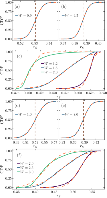
Numerical studies of the Heisenberg chain have been carried out in the sector with the total spin projection . Since does not commute with the Ising Hamiltonian, , we use the full Hilbert space in the latter case. Consequently, in the case of the Heisenberg chain, we may access larger system sizes than for the Ising chain. Figure 1 shows cumulative distribution functions of obtained from multiple realizations of disorder for fixed and various panels correspond to different values of . In both models, results for weak disorder [Figs. 1(a) and 1(d)] or strong disorder [Figs. 1(b) and 1(e)] can be accurately fitted by the error function, and the fits are shown as dashed curves. In both regimes one observes Gaussian sample-to-sample fluctuations centered at (for weak disorder) or (for strong disorder). However, for intermediate disorders [Figs. 1(c) and 1(f)] the distributions visibly deviate from the error functions. In particular, the values of obtained for the Ising model at span almost the whole window between and , see Figs. 1(c). Similar observation holds true also for the Heisenberg model at , as it is shown in Fig. 1(f).
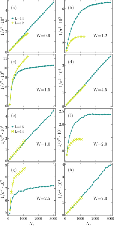
In order to identify the origin of these fluctuations, we calculate the variances of the distributions shown in Fig. 1, , where means averaging over samples of disorder. In Fig. 2 we show how this quantity depends on the number of energy levels, , used for evaluation of for each sample. For weak or strong disorder, the variances scale as while the dependence of on is rather insignificant. This behavior is shown in Figs. 2(a) and 2(d) for the Ising model and in Figs. 2(e) and 2(h) for the Heisenberg chain. Therefore, in the regime of weak or strong disorder the fluctuations of the gap ratio seem to have purely statistical origin which can be linked solely to the number of energy levels which are accessible in finite systems. The correlations between and should not be essential for sufficiently distant and . Then, is a random variable. Its distribution tends toward the normal distribution for large with the variance that is inversely proportional to .
Such picture breaks down for the intermediate disorder strengths, as it can be observed from Figs. 2(b), 2(c) for the Ising model and Figs. 2(f), 2(g) for the Heisenberg chain. The distributions are much broader than for the previously discussed cases, almost saturates for large and shows strong dependence on the system size . Departure of the distribution of from the normal distribution for large suggests that certain realizations of disorder are more relevant for the ”ergodic system” while the others are more relevant for the ”localized system” despite being drawn for the same disorder strength . In other words, we expect that for the accessible system sizes, the sequence is too short to be fully specified by a single quantity, .
In order to test this conjecture and to decrease the sample-to-sample fluctuations of we introduce a new parameter to describe the properties of the random sequence ,
| (3) |
where and are, respectively, the variances of the diagonal and off-diagonal elements of the Hamiltonian matrix, , in the real-space basis . The ratio is rescaled by the dimension of the Hilbert space, , in order to have a non-zero value for .
The result for can be obtained from the high-temperature expansion. In the case of the Heisenberg model, the variance of the off-diagonal part equals, up to the factor, the Hilbert-Schmidt norm of the spin-flip term, . The diagonal variance is determined by the norms of the -term and the random field term, . Since are independent random variables, one finds
| (4) |
where is a random variable which for large is described by a normal distribution with mean zero and the variance . Then, one may calculate for the Heisenberg model in the thermodynamic limit
| (5) |
Similar analysis applied for the Ising chain yields
| (6) |
The properties of a finite system are not determined by but rather by the sequence of random potentials . Then, the question is whether the physical properties of a finite system with a fixed sequence are more accurately encoded in the value of (used to generate the sequence) or in the ratio . In order to answer this question one needs to check whether the sample-to-sample fluctuations are smaller within results obtained for fixed or for fixed . Further on we demonstrate that the latter case holds true. The motivation for discussing comes from that it is directly related to the norm of the perturbation term relatively to the norms of the other terms of the Hamiltonian. In other words, it allows to distinguish ”more localized” samples with larger from ”more ergodic” cases where the latter quantity is smaller. An essential observation following from Eq. (4) is that in the thermodynamic limit there is one-to-one correspondence between the values of and , so the system’s properties are fully specified by either of these quantities. An additional support for using is discussed in the subsequent section, where we introduce a phenomenological model which accurately reproduces broad, non-Gaussian fluctuations of in finite systems.
IV Phenomenological model for the sample-to-sample fluctuation of gap ratio.
Our phenomenological approach is motivated by the Rosenzweig-Porter model [81, 82], where the ergodic-nonergodic crossover originates from different variances of the diagonal and off-diagonal elements of random-matrices. In that model, one considers random matrices, , such that diagonal elements and all off-diagonal elements in the upper triangle of the symmetric matrix are sampled from a normal (Gaussian) distribution with and , respectively, and where the crossover takes place at . In order to account for the finite-size fluctuations discussed in the preceding section, we consider a generalisation to the RP model with sample fluctuations (RPSF), where is not a constant for different samples but rather a random variable that changes from sample to sample. We assume that is drawn from the normal distribution with the variance with the probability density function
| (7) |
Note that despite this generalisation, RPSF model remains a single parameter () model, just like the standard RP model. Within the RP and RPSF models one generates dense matrices where all matrix elements are nonzero. However, in microscopic models discussed in the preceding section, the number of nonzero off-diagonal elements grows as .
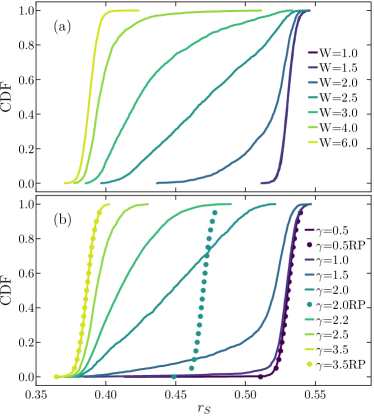
In order to carry out simulations of such model first we draw random and then for fixed and we generate normally distributed real-valued matrix elements. In figure 3 we compare the distributions of obtained for the random-field Heisenberg chain with sites [panel (a)] and for the RP or RPSF models [panel (b)]. In the latter case, we have diagonalized random matrices generated according to the procedure discussed in the preceding paragraph. We recall that in the case of the Heisenberg chain, the dimension of the Hilbert space is approximately 12000. One observes that the standard RP model [points in Fig. 3(b)] correctly captures the distributions of only for parameters which are far away from the GOE/Poisson crossover, i.e., for or . Even though random matrices are smaller than the matrices representing the Heisenberg Hamiltonian, the standard RP model fails to reproduce the broad distributions observed in the vicinity of the crossover at . In contrast, the generalized RPSF model correctly reproduces the numerical studies of the microscopic model for arbitrary . Interestingly, both versions of the RP model give almost indistinguishable results for or . Therefore, the generalization affects predominantly the sample-to-sample fluctuation observed in the vicinity of the crossover.
Next we demonstrate that the sample-to-sample fluctuation in RPSF vanish in the termodynamic limit, , and discuss how these fluctuation depend on the system size. To this end we transform the random variable in Eq. (7) and introduce such that . It is clear that plays that same role in RPSF model as the exponent in the standard RP model except that changes from sample to sample. In order to obtain the probability density function we compare the cumulative distribution functions
| (8) |
where . Differentiating Eq. (8) with respect to one obtains
| (9) |
Note that is normalized and the corresponding cumulative distribution gives where erf is the Gaussian error function. The distribution function approaches the delta function for . Consequently, the standard RP and the RPSF models are equivalent in the thermodynamic limit. One may also find the finite size fluctuations
| (10) |
Interestingly, the standard deviation of decays as the inverse of the linear system’s dimension, , even though such dimension does not explicitly enter the RPSF model. To conclude this section, we note that a simple extension to the RP model allows reproducing the sample-to-sample fluctuations in a finite system, whereas, in the thermodynamic limit, both models (RP and RPSF) are equivalent.
V Numerical results for disordered Ising and Heisenberg chains
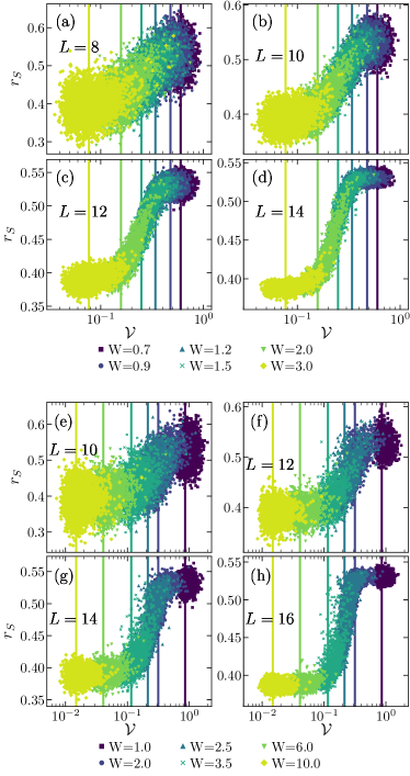
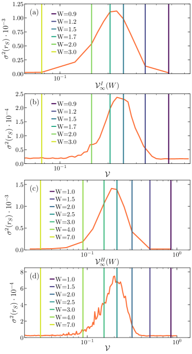
Here we demonstrate that using results from the proceeding section one may reduce sample-to-sample fluctuations also in both microscopic models. In Fig. 4 we show correlations between the gap ratio, , and , see Eq. (3), where both quantities are calculated separately for each disorder realization. We use different symbols to distinguish between disorders drawn for various and vertical guidelines mark [Eq. (6)] and [Eq. (5)] obtained for the Ising and the Heisenberg chains, respectively. One observers that results obtained for various realizations of disorder form a single sigmoid-like curve. The points are scattered in both directions. The vertical scattering means that does not fully specify in finite systems, whereas the horizontal scattering means that does not fully specify . The scattering in the horizontal direction is responsible for fluctuation of which are intensified on the steep section of the sigmoid, i.e, in the vicinity of the crossover between the Poisson and the GOE level statistics.
The latter contribution to may be eliminated once one studies fluctuations for fixed instead of fixed . To this end, in each step of simulations, we first randomly choose , for the Ising chain and for the Heisenberg model, we draw the random fields and then construct the Hamiltonian and obtain and . The results are identical to those in Fig. 4 except that now points almost uniformly cover the entire range of . Then in narrow windows of we calculate the variances, . Results are shown in figures 5(b) and 5(d) for the Ising and Heisenberg chains, respectively. In panels (a) and (c) we show the spreads of distributions in Fig. 1, i.e., distributions generated in a standard way for fixed . In order to facilitate the comparison of both types of results in (a) and (c), we plot vs. and , respectively. For the Ising model, we observe that obtained from fixed is approximately five times smaller than obtained from fixed . In the case of the Heisenberg model, the reduction of fluctuations is less significant but still clearly visible.
Following the suggestion in Ref. [83], we have concentrated our efforts on statistics of energy levels in the crossover regime from GOE to MBL observed on finite–size lattices. There is particular attention devoted to the intermediate crossover regime as it appears on finite lattices in the hope that a better understanding of this regime would yield additional new information about the nature of the MBL phase transition[84, 83] in the thermodynamic limit. Our research was also inspired by the notion that in the regime of strong disorder where the MBL phase is predicted to occur, the finite–size effects critically affect results obtained from exact diagonalization approaches on a small lattice sizes[85, 47, 86]. Our approach demonstrates how to reduce the finite-size sample-to-sample fluctuations and it does not relay on any particular picture that holds in the thermodynamic limit.
VI Conclusions
In finite disordered systems, we have studied the sample-to-sample fluctuations of the gap-ratio, , which are expected to show the GOE/Poisson crossover. In order to single-out generic model-independent properties, we have numerically studied the random-field Heisenberg chains as well as the random-field Ising model. Far from the crossover, the fluctuations of are set by the dimension of the Hilbert space. Consequently, the standard RP model correctly reproduces the fluctuations obtained for microscopic systems. Random matrices of comparable sizes as the matrices of the microscopic Hamiltonians give rise to similar fluctuations. However, this is not the case in the vicinity of the crossover when the fluctuations in the microscopic models significantly exceed the results for the standard RP model. This discrepancy is because the relatively small sets of random fields, may be very different despite being drawn for the same disorder strength, . As a result, specific samples drawn for finite system appear more ergodic while the others are more localized. We have demonstrated that this feature may be implemented in the generalized RP model rather straightforwardly. In its generalized version, i.e, in the RPSF model, the variance of the off-diagonal matrix elements is a normally-distributed random variable that changes from sample to sample. The width of the latter distribution is the same as the constant variance in the standard RP model. The generalized RPSF model accurately captures the distributions of the gap ratio in finite chains essentially for all studied regimes. Moreover, far away from the GOE/Poisson crossovers, both versions of the Rosenzweig-Porter model give almost identical distributions.
Utilizing the latter result, we have demonstrated that the sample-to-sample fluctuations in the finite microscopic model can be reduced. Instead of studying the distributions of the gap ratio for fixed , we have evaluated them in terms of a fixed ratio of the Hilbert Schmidt norms of the diagonal and off-diagonal parts of the Hamiltonian. The norm of the random-field term depends on but also accounts for differences between various realizations of the random fields. The latter ratio of norms is a counterpart of the ratio of variances in the RPSF model. We have shown that this procedure significantly reduces sample-to-sample fluctuations in the Ising model, while the reduction for the Heisenberg model is less pronounced.
Acknowledgements.
We acknowledge the support by the National Science Centre, Poland via project 2020/37/B/ST3/00020 (B.K and M.M.), the support by the Slovenian Research Agency (ARRS), Research Core Fundings Grant P1-0044 (J.B.), and the support from the Center for Integrated Nanotechnologies, a U.S. Department of Energy, Office of Basic Energy Sciences user facility (J.B.). The numerical calculations were partly carried out at the facilities of the Wroclaw Centre for Networking and Supercomputing.References
- Gornyi et al. [2005] I. V. Gornyi, A. D. Mirlin, and D. G. Polyakov, Interacting electrons in disordered wires: Anderson localization and low- transport, Phys. Rev. Lett. 95, 206603 (2005).
- Basko et al. [2006] D. Basko, I. Aleiner, and B. Altshuler, Metal-insulator transition in a weakly interacting many-electron system with localized single-particle states, Ann. Phys. 321, 1126 (2006).
- Oganesyan and Huse [2007] V. Oganesyan and D. A. Huse, Localization of interacting fermions at high temperature, Phys. Rev. B 75, 155111 (2007).
- Abanin et al. [2019] D. A. Abanin, E. Altman, I. Bloch, and M. Serbyn, Colloquium: Many-body localization, thermalization, and entanglement, Rev. Mod. Phys. 91, 021001 (2019).
- Barišić and Prelovšek [2010] O. S. Barišić and P. Prelovšek, Conductivity in a disordered one-dimensional system of interacting fermions, Phys. Rev. B 82, 161106 (2010).
- Luitz et al. [2015] D. J. Luitz, N. Laflorencie, and F. Alet, Many-body localization edge in the random-field Heisenberg chain, Phys. Rev. B 91, 081103 (2015).
- Luitz et al. [2016] D. J. Luitz, N. Laflorencie, and F. Alet, Extended slow dynamical regime close to the many-body localization transition, Phys. Rev. B 93, 060201 (2016).
- Torres-Herrera and Santos [2015] E. J. Torres-Herrera and L. F. Santos, Dynamics at the many-body localization transition, Phys. Rev. B 92, 014208 (2015).
- Andraschko et al. [2014] F. Andraschko, T. Enss, and J. Sirker, Purification and many-body localization in cold atomic gases, Phys. Rev. Lett. 113, 217201 (2014).
- Pal and Huse [2010] A. Pal and D. A. Huse, Many-body localization phase transition, Phys. Rev. B 82, 174411 (2010).
- Bera et al. [2015] S. Bera, H. Schomerus, F. Heidrich-Meisner, and J. H. Bardarson, Many-body localization characterized from a one-particle perspective, Phys. Rev. Lett. 115, 046603 (2015).
- Hauschild et al. [2016] J. Hauschild, F. Heidrich-Meisner, and F. Pollmann, Domain-wall melting as a probe of many-body localization, Physical Review B 94, 161109 (2016).
- Devakul and Singh [2015] T. Devakul and R. R. P. Singh, Early breakdown of area-law entanglement at the many-body delocalization transition, Phys. Rev. Lett. 115, 187201 (2015).
- Bertrand and García-García [2016] C. L. Bertrand and A. M. García-García, Anomalous Thouless energy and critical statistics on the metallic side of the many-body localization transition, Phys. Rev. B 94, 144201 (2016).
- Khemani et al. [2017] V. Khemani, S. P. Lim, D. N. Sheng, and D. A. Huse, Critical properties of the many-body localization transition, Phys. Rev. X 7, 021013 (2017).
- Doggen et al. [2018] E. V. H. Doggen, F. Schindler, K. S. Tikhonov, A. D. Mirlin, T. Neupert, D. G. Polyakov, and I. V. Gornyi, Many-body localization and delocalization in large quantum chains, Phys. Rev. B 98, 174202 (2018).
- Šuntajs et al. [2020a] J. Šuntajs, J. Bonča, T. Prosen, and L. Vidmar, Quantum chaos challenges many-body localization, Phys. Rev. E 102, 062144 (2020a).
- Šuntajs et al. [2020b] J. Šuntajs, J. Bonča, T. Prosen, and L. Vidmar, Ergodicity breaking transition in finite disordered spin chains, Phys. Rev. B 102, 064207 (2020b).
- Kiefer-Emmanouilidis et al. [2020] M. Kiefer-Emmanouilidis, R. Unanyan, M. Fleischhauer, and J. Sirker, Evidence for unbounded growth of the number entropy in many-body localized phases, Phys. Rev. Lett. 124, 243601 (2020).
- Luitz and Lev [2020] D. J. Luitz and Y. B. Lev, Absence of slow particle transport in the many-body localized phase, Phys. Rev. B 102, 100202(R) (2020).
- Abanin et al. [2021] D. Abanin, J. Bardarson, G. De Tomasi, S. Gopalakrishnan, V. Khemani, S. Parameswaran, F. Pollmann, A. Potter, M. Serbyn, and R. Vasseur, Distinguishing localization from chaos: Challenges in finite-size systems, Annals of Physics 427, 168415 (2021).
- Sels and Polkovnikov [2021a] D. Sels and A. Polkovnikov, Dynamical obstruction to localization in a disordered spin chain, Phys. Rev. E 104, 054105 (2021a).
- Sierant et al. [2021] P. Sierant, E. Gonzalez Lazo, M. Dalmonte, A. Scardicchio, and J. Zakrzewski, Constraints induced delocalization, arXiv e-prints , arXiv:2103.14020 (2021), arXiv:2103.14020 [cond-mat.dis-nn] .
- Vidmar et al. [2021] L. Vidmar, B. Krajewski, J. Bonča, and M. Mierzejewski, Phenomenology of spectral functions in disordered spin chains at infinite temperature, Phys. Rev. Lett. 127, 230603 (2021).
- Sels and Polkovnikov [2021b] D. Sels and A. Polkovnikov, Thermalization through linked conducting clusters in spin chains with dilute defects (2021b), arXiv:2105.09348 [quant-ph] .
- Morningstar et al. [2021] A. Morningstar, L. Colmenarez, V. Khemani, D. J. Luitz, and D. A. Huse, Avalanches and many-body resonances in many-body localized systems (2021), arXiv:2107.05642 [cond-mat.dis-nn] .
- Sels [2021] D. Sels, Markovian baths and quantum avalanches (2021), arXiv:2108.10796 [cond-mat.dis-nn] .
- Kiefer-Emmanouilidis et al. [2021] M. Kiefer-Emmanouilidis, R. Unanyan, M. Fleischhauer, and J. Sirker, Unlimited growth of particle fluctuations in many-body localized phases, Annals of Physics , 168481 (2021).
- Deutsch [1991] J. M. Deutsch, Quantum statistical mechanics in a closed system, Phys. Rev. A 43, 2046 (1991).
- Srednicki [1994] M. Srednicki, Chaos and quantum thermalization, Phys. Rev. E 50, 888 (1994).
- Rigol et al. [2008] M. Rigol, V. Dunjko, and M. Olshanii, Thermalization and its mechanism for generic isolated quantum systems, Nature (London) 452, 854 (2008).
- D’Alessio et al. [2016] L. D’Alessio, Y. Kafri, A. Polkovnikov, and M. Rigol, From quantum chaos and eigenstate thermalization to statistical mechanics and thermodynamics, Adv. Phys. 65, 239 (2016).
- Mori et al. [2018] T. Mori, T. N. Ikeda, E. Kaminishi, and M. Ueda, Thermalization and prethermalization in isolated quantum systems: a theoretical overview, J. Phys. B 51, 112001 (2018).
- Deutsch [2018] J. M. Deutsch, Eigenstate thermalization hypothesis, Rep. Prog. Phys. 81, 082001 (2018).
- Santos and Rigol [2010] L. F. Santos and M. Rigol, Onset of quantum chaos in one-dimensional bosonic and fermionic systems and its relation to thermalization, Phys. Rev. E 81, 036206 (2010).
- Beugeling et al. [2014] W. Beugeling, R. Moessner, and M. Haque, Finite-size scaling of eigenstate thermalization, Phys. Rev. E 89, 042112 (2014).
- Steinigeweg et al. [2014] R. Steinigeweg, A. Khodja, H. Niemeyer, C. Gogolin, and J. Gemmer, Pushing the limits of the eigenstate thermalization hypothesis towards mesoscopic quantum systems, Phys. Rev. Lett. 112, 130403 (2014).
- Kim et al. [2014] H. Kim, T. N. Ikeda, and D. A. Huse, Testing whether all eigenstates obey the eigenstate thermalization hypothesis, Phys. Rev. E 90, 052105 (2014).
- Mondaini and Rigol [2017] R. Mondaini and M. Rigol, Eigenstate thermalization in the two-dimensional transverse field Ising model. II. Off-diagonal matrix elements of observables, Phys. Rev. E 96, 012157 (2017).
- Jansen et al. [2019] D. Jansen, J. Stolpp, L. Vidmar, and F. Heidrich-Meisner, Eigenstate thermalization and quantum chaos in the Holstein polaron model, Phys. Rev. B 99, 155130 (2019).
- LeBlond et al. [2019] T. LeBlond, K. Mallayya, L. Vidmar, and M. Rigol, Entanglement and matrix elements of observables in interacting integrable systems, Phys. Rev. E 100, 062134 (2019).
- Mierzejewski and Vidmar [2020] M. Mierzejewski and L. Vidmar, Quantitative impact of integrals of motion on the eigenstate thermalization hypothesis, Phys. Rev. Lett. 124, 040603 (2020).
- Brenes et al. [2020] M. Brenes, T. LeBlond, J. Goold, and M. Rigol, Eigenstate Thermalization in a Locally Perturbed Integrable System, Phys. Rev. Lett. 125, 070605 (2020).
- Richter et al. [2020] J. Richter, A. Dymarsky, R. Steinigeweg, and J. Gemmer, Eigenstate thermalization hypothesis beyond standard indicators: Emergence of random-matrix behavior at small frequencies, Phys. Rev. E 102, 042127 (2020).
- [45] C. Schönle, D. Jansen, F. Heidrich-Meisner, and L. Vidmar, Eigenstate thermalization hypothesis through the lens of autocorrelation functions, arXiv:2011.13958.
- [46] M. Brenes, S. Pappalardi, M. T. Mitchison, J. Goold, and A. Silva, Out-of-time-order correlations and the fine structure of eigenstate thermalisation, arXiv:2103.01161.
- Panda et al. [2020] R. K. Panda, A. Scardicchio, M. Schulz, S. R. Taylor, and M. Žnidarič, Can we study the many-body localisation transition?, EPL (Europhysics Letters) 128, 67003 (2020).
- Corps et al. [2021] Á. L. Corps, R. A. Molina, , and A. Relaño, Signatures of a critical point in the many-body localization transition, SciPost Phys. 10, 107 (2021).
- Gray et al. [2018] J. Gray, S. Bose, and A. Bayat, Many-body localization transition: Schmidt gap, entanglement length, and scaling, Phys. Rev. B 97, 201105 (2018).
- Schiulaz et al. [2019] M. Schiulaz, E. J. Torres-Herrera, and L. F. Santos, Thouless and relaxation time scales in many-body quantum systems, Phys. Rev. B 99, 174313 (2019).
- Žnidarič et al. [2008] M. Žnidarič, T. Prosen, and P. Prelovšek, Many-body localization in the Heisenberg XXZ magnet in a random field, Phys. Rev. B 77, 064426 (2008).
- Bardarson et al. [2012] J. H. Bardarson, F. Pollmann, and J. E. Moore, Unbounded growth of entanglement in models of many-body localization, Phys. Rev. Lett. 109, 017202 (2012).
- Kjäll et al. [2014] J. A. Kjäll, J. H. Bardarson, and F. Pollmann, Many-body localization in a disordered quantum Ising chain, Phys. Rev. Lett. 113, 107204 (2014).
- Serbyn et al. [2015] M. Serbyn, Z. Papić, and D. A. Abanin, Criterion for many-body localization-delocalization phase transition, Phys. Rev. X 5, 041047 (2015).
- Serbyn et al. [2013] M. Serbyn, Z. Papić, and D. A. Abanin, Universal slow growth of entanglement in interacting strongly disordered systems, Phys. Rev. Lett. 110, 260601 (2013).
- Altman and Vosk [2015] E. Altman and R. Vosk, Universal dynamics and renormalization in many-body-localized systems, Annu. Rev. Condens. Matter Phys. 6, 383 (2015).
- Agarwal et al. [2015] K. Agarwal, S. Gopalakrishnan, M. Knap, M. Müller, and E. Demler, Anomalous diffusion and Griffiths effects near the many-body localization transition, Phys. Rev. Lett. 114, 160401 (2015).
- Gopalakrishnan et al. [2015] S. Gopalakrishnan, M. Müller, V. Khemani, M. Knap, E. Demler, and D. A. Huse, Low-frequency conductivity in many-body localized systems, Phys. Rev. B 92, 104202 (2015).
- Žnidarič et al. [2016] M. Žnidarič, A. Scardicchio, and V. K. Varma, Diffusive and Subdiffusive Spin Transport in the Ergodic Phase of a Many-Body Localizable System, Phys. Rev. Lett. 117, 040601 (2016).
- Mierzejewski et al. [2016] M. Mierzejewski, J. Herbrych, and P. Prelovšek, Universal dynamics of density correlations at the transition to the many-body localized state, Phys. Rev. B 94, 224207 (2016).
- Bar Lev and Reichman [2014] Y. Bar Lev and D. R. Reichman, Dynamics of many-body localization, Phys. Rev. B 89, 220201 (2014).
- Bar Lev et al. [2015] Y. Bar Lev, G. Cohen, and D. R. Reichman, Absence of diffusion in an interacting system of spinless fermions on a one-dimensional disordered lattice, Phys. Rev. Lett. 114, 100601 (2015).
- Barišić et al. [2016] O. S. Barišić, J. Kokalj, I. Balog, and P. Prelovšek, Dynamical conductivity and its fluctuations along the crossover to many-body localization, Phys. Rev. B 94, 045126 (2016).
- Bonča and Mierzejewski [2017] J. Bonča and M. Mierzejewski, Delocalized carriers in the t-J model with strong charge disorder, Phys. Rev. B 95, 214201 (2017).
- Bordia et al. [2017] P. Bordia, H. Lüschen, S. Scherg, S. Gopalakrishnan, M. Knap, U. Schneider, and I. Bloch, Probing slow relaxation and many-body localization in two-dimensional quasiperiodic systems, Phys. Rev. X 7, 041047 (2017).
- Sierant et al. [2017] P. Sierant, D. Delande, and J. Zakrzewski, Many-body localization due to random interactions, Phys. Rev. A 95, 021601 (2017).
- Protopopov and Abanin [2019] I. V. Protopopov and D. A. Abanin, Spin-mediated particle transport in the disordered Hubbard model, Phys. Rev. B 99, 115111 (2019).
- Schecter et al. [2018] M. Schecter, T. Iadecola, and S. Das Sarma, Configuration-controlled many-body localization and the mobility emulsion, Phys. Rev. B 98, 174201 (2018).
- Zakrzewski and Delande [2018] J. Zakrzewski and D. Delande, Spin-charge separation and many-body localization, Phys. Rev. B 98, 014203 (2018).
- Khait et al. [2016] I. Khait, S. Gazit, N. Y. Yao, and A. Auerbach, Spin transport of weakly disordered Heisenberg chain at infinite temperature, Phys. Rev. B 93, 224205 (2016).
- Luitz and Lev [2017] D. J. Luitz and Y. B. Lev, The ergodic side of the many-body localization transition, Annalen der Physik 529, 1600350 (2017).
- Bera et al. [2017] S. Bera, G. De Tomasi, F. Weiner, and F. Evers, Density Propagator for Many-Body Localization: Finite-Size Effects, Transient Subdiffusion, and Exponential Decay, Phys. Rev. Lett. 118, 196801 (2017).
- Kozarzewski et al. [2018] M. Kozarzewski, P. Prelovšek, and M. Mierzejewski, Spin subdiffusion in the disordered Hubbard chain, Phys. Rev. Lett. 120, 246602 (2018).
- Prelovšek and Herbrych [2017] P. Prelovšek and J. Herbrych, Self-consistent approach to many-body localization and subdiffusion, Phys. Rev. B 96, 035130 (2017).
- Prelovšek et al. [2018] P. Prelovšek, J. Bonča, and M. Mierzejewski, Transient and persistent particle subdiffusion in a disordered chain coupled to bosons, Phys. Rev. B 98, 125119 (2018).
- Serbyn et al. [2017] M. Serbyn, Z. Papić, and D. A. Abanin, Thouless energy and multifractality across the many-body localization transition, Phys. Rev. B 96, 104201 (2017).
- Mierzejewski et al. [2020] M. Mierzejewski, M. Środa, J. Herbrych, and P. Prelovšek, Resistivity and its fluctuations in disordered many-body systems: From chains to planes, Phys. Rev. B 102, 161111 (2020).
- Weiner et al. [2019] F. Weiner, F. Evers, and S. Bera, Slow dynamics and strong finite-size effects in many-body localization with random and quasiperiodic potentials, Phys. Rev. B 100, 104204 (2019).
- Sierant and Zakrzewski [2019] P. Sierant and J. Zakrzewski, Level statistics across the many-body localization transition, Phys. Rev. B 99, 104205 (2019).
- Sierant and Zakrzewski [2020] P. Sierant and J. Zakrzewski, Model of level statistics for disordered interacting quantum many-body systems, Phys. Rev. B 101, 104201 (2020).
- Rosenzweig and Porter [1960] N. Rosenzweig and C. E. Porter, ”Repulsion of Energy Levels” in Complex Atomic Spectra, Phys. Rev. 120, 1698 (1960).
- Pino et al. [2019] M. Pino, J. Tabanera, and P. Serna, From ergodic to non-ergodic chaos in Rosenzweig–Porter model, Journal of Physics A: Mathematical and Theoretical 52, 475101 (2019).
- Morningstar et al. [2022] A. Morningstar, L. Colmenarez, V. Khemani, D. J. Luitz, and D. A. Huse, Avalanches and many-body resonances in many-body localized systems, Phys. Rev. B 105, 174205 (2022).
- Crowley and Chandran [2020] P. J. D. Crowley and A. Chandran, A constructive theory of the numerically accessible many-body localized to thermal crossover 10.48550/ARXIV.2012.14393 (2020).
- Sierant et al. [2020] P. Sierant, D. Delande, and J. Zakrzewski, Thouless time analysis of anderson and many-body localization transitions, Phys. Rev. Lett. 124, 186601 (2020).
- Ware et al. [2021] B. Ware, D. Abanin, and R. Vasseur, Perturbative instability of nonergodic phases in non-abelian quantum chains, Phys. Rev. B 103, 094203 (2021).