Critical Endpoint of QCD and Baryon Number Fluctuations in a Finite Volume

Abstract

We summarize recent results on the volume dependence of the location of the critical endpoint in the QCD phase diagram. To this end, we employ a sophisticated combination of Lattice Yang–Mills theory and a (truncated) version of Dyson–Schwinger equations in Landau gauge for $2+1$ quark flavours. We study this system at small and intermediate volumes and determine the dependence of the location of the critical endpoint on the boundary conditions and the volume of a three-dimensional cube with edge length $L$. We also discuss recent results on baryon number fluctuations in this setup.

1 Introduction

One of the prime goals of many heavy-ion collision experiments is to verify the existence and determine the location of the putative critical endpoint (CEP) in the phase diagram of QCD. However, the hot and dense QCD matter formed in these experiments is only finite in spatial extent, which depends, e.g., on the size of the colliding ions and the centrality of the collision. As a consequence, it serves as an important cross-check between theory and experiment to analyse potential dependences of the experimental signatures on this finite volume in theoretical calculations. To this end, it is especially interesting to investigate the fluctuations of conserved charges such as the baryon number.

In the following, we summarize our findings for the QCD phase diagram in a finite volume obtained from Dyson–Schwinger equations (DSEs) as found in Ref. [1]. Additionally, we present very recent results from Ref. [2] for the finite-volume baryon number fluctuations around the CEP in the same framework.

2 Dyson–Schwinger Equations

For all following investigations, the main quantity of interest is the nonperturbative quark propagator $S_{f}$ of quark flavour $f\in\{\mathrm{u}/\mathrm{d},\mathrm{s}\}$ – i.e., a $2+1$ flavour setup – at temperature $T$ and quark chemical potential $\mu_{f}$. It is calculated using DSEs which are the quantum equations of motion for the correlation functions of a quantum field theory. While in principle not requiring any approximations, they imply an infinite tower of coupled equations that has to be truncated for practical calculations.

We use a truncation that has been used extensively for investigations of the QCD phase diagram in the past (see, e.g., our recent works in Refs. [3, 4, 5, 6, 1, 2]). That is, we solve the DSEs for the quark and gluon propagators using a model ansatz for the quark–gluon vertex. For the gluon, we employ quenched lattice data and take unquenching effects into account by calculating the quark loop explicitly. For the sake of brevity, we refer the reader to the review [7] and references therein for explicit expressions and more details.

3 Finite-Volume Framework

In order to specify a three-dimensional finite-volume framework, we need to fix both a shape and the boundary conditions of the volume. A mathematically feasible choice is a cube with edge length $L$ and antiperiodic/periodic spatial boundary conditions (ABC/PBC). As a consequence, each component in momentum space can only assume discrete values of the spatial Matsubara modes,

$$\omega_{n}^{L}=\frac{\uppi}{L}\times\begin{cases}2n&\text{for PBC}\,,\\ 2n+1&\text{for ABC}\,,\end{cases}\quad n\in\mathbb{Z}\,,$$ (1)

and all momentum integrals in our DSEs become sums, which is the central relation of our setup:

$$\int\frac{\mathrm{d}^{3}q}{(2\uppi)^{3}}\,K(\vec{q})\,\to\,\frac{1}{L^{3}}\sum_{\vec{n}\in\mathbb{Z}^{3}}K(\vec{q}_{\vec{n}})\,,\ \text{ with }\ \vec{q}_{\vec{n}}:=\sum_{i=1}^{3}\omega^{L}_{n_{i}}\vec{e}_{i}\,,$$ (2)

for a generic integrand $K$. For practical calculations, however, more intricacies have to be taken care of which is described in detail in Ref. [1].

4 Results

QCD Phase Diagram

We start our investigation of the QCD phase diagram with the volume dependence of crossover line and CEP as performed in Ref. [1]. To this end, we employ the quark condensate as the order parameter for chiral symmetry breaking which in our setup reads

$$\langle\overline{\psi}\psi\rangle_{f}\sim-\frac{T}{L^{3}}\sum_{\omega_{m}}\sum_{\vec{n}\in\mathbb{Z}^{3}}\,\operatorname{Tr}\bigl{[}S_{f}(\omega_{m}+\mathrm{i}\mu_{f},\vec{q}_{\vec{n}})\bigr{]}\,,$$ (3)

where $\omega_{m}$ are the temporal Matsubara frequencies introduced by the temperature. For any nonvanishing bare quark mass, the condensate is divergent and needs to be regularized. To this end, we define the subtracted condensate, $\Delta_{\mathrm{u}\mathrm{s}}:=\langle\overline{\psi}\psi\rangle_{\mathrm{u}}-(m_{\mathrm{u}}/m_{\mathrm{s}})\langle\overline{\psi}\psi\rangle_{\mathrm{s}}$. The pseudocritical temperature of the chiral crossover transition is in our case defined as the inflection point of $\Delta_{\mathrm{u}\mathrm{s}}$ with respect to temperature, while the CEP is the point where the crossover becomes second order.

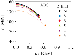
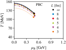
Figure 1: Finite-volume effects on the QCD phase diagram for antiperiodic (left) and periodic (right) boundary conditions and different box sizes. Here, we show the crossover lines and locations of the CEPs (symbols).

In Figure 1, we show our findings for the QCD phase diagram for both boundary conditions and systems sizes between $L=$3\text{\,}\mathrm{fm}$$ and $L=$8\text{\,}\mathrm{fm}$$ with $L\to\infty$ as a reference. We find a consistent infinite-volume limit, i.e., the $L=$8\text{\,}\mathrm{fm}$$ results are almost indistinguishable from the $L\to\infty$ ones. Visible volume effects start to appear below $L\lesssim$4\text{\,}\mathrm{fm}$$, while for larger system sizes, the results are very close to one another and basically identical for both boundary conditions. In general, the crossover lines move towards lower temperatures for decreasing system sizes. Except for PBC and $L=$3\text{\,}\mathrm{fm}$$, the CEPs also tend to move in direction of higher chemical potentials.

Baryon Number Fluctuations

Next, we turn to the analysis of baryon number fluctuations around the CEP as we did in Ref. [2]. Our starting point are the quark number fluctuations,

$$\chi_{ijk}^{\mathrm{u}\mathrm{d}\mathrm{s}}=-\frac{1}{T^{4-(i+j+k)}}\,\frac{\partial^{i+j+k}\hskip 0.83344pt\Omega}{\partial\mu_{\mathrm{u}}^{i}\hskip 0.83344pt\partial\mu_{\mathrm{d}}^{j}\hskip 0.83344pt\partial\mu_{\mathrm{s}}^{k}}\,,$$ (4)

which can be related to the ones for the conserved charges baryon number (B), electrical charge (Q) and strangeness (S). As a consequence, the corresponding fluctuations $\chi_{ijk}^{\mathrm{B}\mathrm{Q}\mathrm{S}}$ can be expressed as linear combinations of quark number fluctuations; see Ref. [2] for details.

Baryon number fluctuations are an interesting quantity to study for a number of reasons. For instance, they are rather sensitive to and show signatures of phase transitions and the CEP, and can be related to the moments of the net-baryon distribution accessible in experiments, e.g., $\chi_{3}^{\mathrm{B}}/\chi_{2}^{\mathrm{B}}=S_{\mathrm{B}}\sigma_{\mathrm{B}}$, $\chi_{4}^{\mathrm{B}}/\chi_{2}^{\mathrm{B}}=\kappa_{\mathrm{B}}\hskip 0.83344pt\sigma_{\mathrm{B}}^{2}$, … Additonally, the fluctuations themselves explicitly depend on the system volume while their ratios are expected not to. For more information on fluctuations, see the review [8].

While the QCD grand potential $\Omega$ is inaccessible with DSEs, we can obtain the quark number fluctuations by means of derivatives of the quark number densities $n_{f}$ from the quark propagator,

$$n_{f}=-\frac{\partial\Omega}{\partial\mu_{f}}\sim-\frac{T}{L^{3}}\sum_{\omega_{m}}\sum_{\vec{n}\in\mathbb{Z}^{3}}\,\operatorname{Tr}\bigl{[}\gamma_{4}S_{f}(\omega_{n}+\mathrm{i}\mu_{f},\vec{q}_{\vec{n}})\bigr{]}\,.$$ (5)

In numerical calculations, this expression for the quark number density is divergent and needs to be regularized. In our finite-volume framework, this process is somewhat elaborate which is why we refer the reader to Ref. [2] for details.

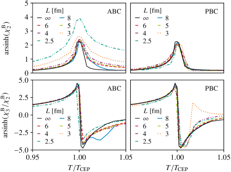
Figure 2: Second order baryon number fluctuations (top row) and skewness ratio (bottom row) against normalized temperature for antiperiodic (left) and periodic (right) boundary conditions in different box sizes $L$. All results are obtained at the critical chemical potential for the respective system size $\mu=\mu_{\textup{CEP}}(L)$.

In Figure 2, we display our results for both the second order baryon number fluctuations (top row) and the skewness ratio (bottom row) around the CEP for both boundary conditions and system sizes between $L=$2.5\text{\,}\mathrm{fm}$$ and $L=$8\text{\,}\mathrm{fm}$$ with $L\to\infty$ for comparison. The main result we find is that the baryon number fluctuations themselves show visible volume effects – especially for ABC – while the ratios are indeed basically independent of the system size. This implies that not only the explicit volume dependence in the ratios cancels but also the implicit one.

5 Acknowledgements

We thank Bernd-Jochen Schaefer for fruitful collaboration on the QCD phase diagram in a finite volume, Ref. [1]. This work has been supported by the Helmholtz Graduate School for Hadron and Ion Research for FAIR, the GSI Helmholtzzentrum für Schwerionenforschung, and the BMBF under Contract No. 05P18RGFCA.

References

- [1] J. Bernhardt, C.S. Fischer, P. Isserstedt and B.-J. Schaefer, Critical endpoint of QCD in a finite volume, Phys. Rev. D 104 (2021) 074035 [2107.05504].
- [2] J. Bernhardt, C.S. Fischer and P. Isserstedt, Finite-volume effects in baryon number fluctuations around the QCD critical endpoint, 2208.01981.
- [3] P. Isserstedt, M. Buballa, C.S. Fischer and P.J. Gunkel, Baryon number fluctuations in the QCD phase diagram from Dyson-Schwinger equations, Phys. Rev. D 100 (2019) 074011 [1906.11644].
- [4] P.J. Gunkel, C.S. Fischer and P. Isserstedt, Quarks and light (pseudo-)scalar mesons at finite chemical potential, Eur. Phys. J. A 55 (2019) 169 [1907.08110].
- [5] P. Isserstedt, C.S. Fischer and T. Steinert, Thermodynamics from the quark condensate, Phys. Rev. D 103 (2021) 054012 [2012.04991].
- [6] P.J. Gunkel and C.S. Fischer, Locating the critical endpoint of QCD: Mesonic backcoupling effects, Phys. Rev. D 104 (2021) 054022 [2106.08356].
- [7] C.S. Fischer, QCD at finite temperature and chemical potential from Dyson–Schwinger equations, Prog. Part. Nucl. Phys. 105 (2019) 1 [1810.12938].
- [8] X. Luo and N. Xu, Search for the QCD Critical Point with Fluctuations of Conserved Quantities in Relativistic Heavy-Ion Collisions at RHIC : An Overview, Nucl. Sci. Tech. 28 (2017) 112 [1701.02105].