Inferring physical properties of symmetric states from the fewest copies

Abstract

Learning physical properties of high-dimensional states is crucial for developing quantum technologies but usually consumes an exceedingly large number of samples which are difficult to afford in practice. In this Letter, we use the methodology of quantum metrology to tackle this difficulty, proposing a strategy built upon entangling measurements for dramatically reducing sample complexity. The strategy, whose characteristic feature is symmetrization of observables, is powered by the exploration of symmetric structures of states which are ubiquitous in physics. It is provably optimal under some natural assumption, efficiently implementable in a variety of contexts, and capable of being incorporated into existing methods as a basic building block. We apply the strategy to different scenarios motivated by experiments, demonstrating exponential reductions in sample complexity.

Learning properties of states like expectation values of observables is of increasing importance in quantum physics, underpinning vast applications in emerging fields, such as quantum machine learning Biamonte et al. (2017), quantum computational chemistry McArdle et al. (2020), and variational quantum computing Cerezo et al. (2021); Tilly et al. (2022). A fundamental difficulty in this task is that any full reconstruction of a generic unknown state inevitably consumes exponentially many samples due to the growth of the state space dimension with the system size. This makes traditional learning methods like full state tomography hopelessly inefficient and poses a serious challenge in the Noisy Intermediate-Scale Quantum (NISQ) era Preskill (2018).

Fortunately, although there are a large number of states in the state space, most of the physically relevant states are the ones that admit some nontrivial structures, such as those of low rank Gross et al. (2010); Liu et al. (2012), matrix product states Cramer et al. (2010); Baumgratz et al. (2013), and those with quasi-local structures Anshu et al. (2021); Rouzé and França (2021). Furthermore, for many purposes, one is only interested in some specific properties of states, e.g., mean energies of many-body systems, which makes it unnecessary to fully reconstruct states for obtaining all their information. These well-motivated physical considerations have led to a series of proposals for more efficient alternatives to full state tomography, with excellent examples including compressed sensing Gross et al. (2010); Liu et al. (2012), adaptive tomography Mahler et al. (2013); Qi et al. (2017), self-guided tomography Ferrie (2014); Rambach et al. (2021), and classical shadow Aaronson (2018); Huang et al. (2020).

While existing methods generally rely on local measurements, it has been recognized that entangling measurements are typically far more efficient than local measurements for extracting information from unknown states Peres and Wootters (1991); Gisin and Popescu (1999); et al. (2022a); Aharonov et al. (2022); Miguel-Ramiro et al. (2022); Larocca et al. (2022). Moreover, the ongoing development of large-scale quantum computers opens up exciting possibilities of leveraging quantum computational resources to realize entangling measurements et al. (2022a); Aharonov et al. (2022). In particular, motivated by the availability of NISQ computers et al. (2022b), a number of experiments Tang et al. (2020); Huang et al. (2022); Conlon et al. (2023) have been carried out for realizing entangling measurements as well as demonstrating their superiority over local measurements. An important issue following is therefore to explore the usefulness of entangling measurements in learning properties of states et al. (2022a); Aharonov et al. (2022).

Here we propose a strategy built upon entangling measurements, for dramatically reducing sample complexity beyond what can be achieved with local measurements. The basic idea is to explore symmetric structures of states which are ubiquitous in physics (see also Ref. Tóth et al. (2010)). Using information-theoretic tools from quantum metrology Helstrom (1976); Holevo (2011), we figure out the measurement that can make best use of these symmetric structures for learning expectation values of observables. This enables our strategy to operate at the optimal sample efficiency in a variety of physical contexts, thereby achieving a sought-after goal in quantum metrology Braunstein and Caves (1994); Zhang and Gong (2020); Zhang and Tong (2022), which is unlikely, if not impossible, to reach with local measurements. Taking translational and permutational symmetries as two examples, we demonstrate that our strategy, when incorporating known efficient quantum circuits, allows for saving exponentially many samples while merely consuming polynomial amounts of quantum computational resources. The findings of this Letter uncover an intriguing route to reducing sample complexity via taking advantage of symmetric structures of states, which opens opportunities for leveraging recent breakthroughs on large-scale quantum computers to accomplish a plethora of learning tasks.

We start with a simple example. Let $\rho$ be an unknown state of a qubit whose symmetric structures are described by the group ${G}=\{\openone,\sigma_{z}\}$, i.e., $\sigma_{z}\rho\sigma_{z}=\rho$, where $\sigma_{\alpha}$, $\alpha=x,y,z$, denote the Pauli matrices. Any observable $X$ of the qubit can be written as $X=a\openone+\bm{b}\cdot\bm{\sigma}$, with $a\in\mathbb{R}$, $\bm{b}=(b_{x},b_{y},b_{z})\in\mathbb{R}^{3}$, and $\bm{\sigma}=(\sigma_{x},\sigma_{y},\sigma_{z})$. To obtain the expectation value $\expectationvalue{X}_{\rho}$ of $X$ in $\rho$, the commonly used approach is to perform the projective measurement of $X$. The quantum uncertainty in this measurement is $(\Delta X)^{2}:=\expectationvalue{X^{2}}_{\rho}-\expectationvalue{X}_{\rho}^{2}$. Resorting to the symmetric structures of $\rho$, we can alternatively measure $Y=\frac{1}{2}X+\frac{1}{2}\sigma_{z}X\sigma_{z}=a\openone+\bm{b}^{\prime}\cdot\bm{\sigma}$ for obtaining $\expectationvalue{X}_{\rho}$, where $\bm{b}^{\prime}=\left(0,0,b_{z}\right)$. The subtle difference between $X$ and $Y$ is that, whereas $\expectationvalue{X}_{\rho}=\expectationvalue{Y}_{\rho}$, $(\Delta X)^{2}=\norm{\bm{b}}^{2}-(a-\expectationvalue{X}_{\rho})^{2}\geq\norm{\bm{b}^{\prime}}^{2}-(a-\expectationvalue{Y}_{\rho})^{2}=(\Delta Y)^{2}$, where $\norm{\cdot}$ denotes the Euclidean norm. So, for obtaining $\expectationvalue{X}_{\rho}$ up to a certain desired precision, the projective measurement of $Y$ generally consumes less copies of $\rho$ than that of $X$. We are thus led to the observation that the expectation value of a given observable may be obtained more efficiently through measuring another observable than the given one when the state in question admits some symmetric structures. Below, we systematically analyze how to optimally take advantage of symmetric structures of states for efficiently learning expectation values of observables.

We consider the general setting that $\rho$ is an unknown state of a (possibly many-body) system with the symmetric structures described by a finite or compact Lie group $G$, i,e, $U_{g}\rho U_{g}^{\dagger}=\rho$ for $g\in G$, where $U_{g}$ denotes a unitary representation of ${G}$. It is worth noting that the majority of symmetric structures of interest in quantum physics can be described in this way. Our aim is to consume as few copies of $\rho$ as possible to learn the expectation value $\expectationvalue{X}_{\rho}$ of any given observable $X$ up to a certain desired precision.

To reach this aim, we resort to the methodology of quantum metrology Helstrom (1976); Holevo (2011) which provides powerful tools to deal with the so-called parameter estimation problems SM . We first set the stage of our analysis. Throughout, we assume that we know nothing about $\rho$ except its symmetric structures, leaving the discussion on this assumption to the end of this Letter. We treat $\expectationvalue{X}_{\rho}$ as the parameter to be estimated and use $\beta$ to represent $\expectationvalue{X}_{\rho}$ for later convenience. Without loss of generality, we can describe the task of learning $\expectationvalue{X}_{\rho}$ from multiple copies of $\rho$ as first performing a measurement on $\rho^{\otimes M}$ and then inferring the value of $\beta=\expectationvalue{X}_{\rho}$ from the measurement outcome et al. (2022a). Here, $M$ denotes the number of samples consumed, which is to be determined shortly. Any measurement can be described by a positive operator-valued measure (POVM) $\{\Pi_{\bm{y}}\}_{\bm{y}}$ satisfying $\sum_{\bm{y}}\Pi_{\bm{y}}=\openone$, where $\bm{y}$ labels the measurement outcome and could be multivariate in general. Any inference rule amounts to finding an estimator $\hat{\beta}(\bm{y})$, which is a map from the set of measurement outcomes to the set of possible values of $\beta$. $\hat{\beta}$ is said to be unbiased if its expected value equals to $\beta$, that is, $\sum_{\bm{y}}p_{\bm{y}}\hat{\beta}(\bm{y})=\beta$, where $p_{\bm{y}}=\tr(\Pi_{\bm{y}}\rho^{\otimes M})$ denotes the probability of getting outcome $\bm{y}$. Associated with a POVM $\{\Pi_{\bm{y}}\}_{\bm{y}}$ and an (unbiased) estimator $\hat{\beta}$, the error in estimating $\beta$ can be quantified by the variance $\textrm{Var}[\hat{\beta}]$ of the estimator $\hat{\beta}$ Helstrom (1976); Holevo (2011), $\textrm{Var}[\hat{\beta}]=\sum_{\bm{y}}p_{\bm{y}}[\hat{\beta}(\bm{y})-\beta]^{2}$. We require that $\textrm{Var}[\hat{\beta}]\leq\epsilon$, where $\epsilon$ characterizes the desired precision.

We next introduce fundamental bounds on $\textrm{Var}[\hat{\beta}]$ and $M$. Using representation theory of groups, we can characterize $\rho$ in terms of some unknown parameters, $\rho=\rho(\bm{\theta})$, with $\bm{\theta}=(\theta_{1},\cdots,\theta_{\mathfrak{p}})$ [see Supplemental Material (SM) SM for details]. This enables us to introduce a bound on $\textrm{Var}[\hat{\beta}]$,

$$\textrm{Var}[\hat{\beta}]\geq\frac{\partial\beta[H(\bm{\theta})]^{-1}\partial\beta^{T}}{M},$$ (1)

known as the quantum Cramér-Rao bound (QCRB) Braunstein and Caves (1994); Zhang and Gong (2020); Zhang and Tong (2022). Here, $\partial\beta=(\partial\beta/\partial\theta_{1},\cdots,\partial\beta/\partial\theta_{\mathfrak{p}})$ and $H(\bm{\theta})$ is a $\mathfrak{p}\times\mathfrak{p}$ symmetric matrix known as the quantum Fisher information matrix. The $kl$ element of $H(\bm{\theta})$ is given by $H_{kl}=\tr[\rho(\bm{\theta})(L_{k}\circ L_{l})]$, where $L_{k}\circ L_{l}=(L_{k}L_{l}+L_{l}L_{k})/2$ denotes the Jordan product, and $L_{k}$ is the symmetric logarithmic derivative defined as the Hermitian operator satisfying $\partial\rho(\bm{\theta})/\partial\theta_{k}=L_{k}\circ\rho(\bm{\theta})$. The meaning of Eq. (1) is that the precision attainable in any task of learning $\beta$ from the $M$ samples is fundamentally constrained by the QCRB Braunstein and Caves (1994); Zhang and Gong (2020); Zhang and Tong (2022), irrespective of the choices of a POVM and an estimator. Inserting $\textrm{Var}[\hat{\beta}]\leq\epsilon$ into Eq. (1), we have

$$M\geq\frac{\partial\beta[H(\bm{\theta})]^{-1}\partial\beta^{T}}{\epsilon},$$ (2)

implying that quantum mechanics does not allow for consuming less than $M_{\textrm{min}}:=\lceil\frac{\partial\beta[H(\bm{\theta})]^{-1}\partial\beta^{T}}{\epsilon}\rceil$ samples for reaching the desired precision. Here $\lceil\cdot\rceil$ denotes the ceiling function.

We then analyze the saturation conditions of the bounds. We derive in SM SM the following crucial equality

$$\partial\beta[H(\bm{\theta})]^{-1}\partial\beta^{T}=(\Delta Y)^{2},$$ (3)

which connects the QCRB to the quantum uncertainty of the observable

$$Y=\mathcal{T}(X).$$ (4)

Here, $\mathcal{T}$ is the $G$-twirling operation defined as $\mathcal{T}(X)=\int_{G}d\nu(g)U_{g}XU_{g}^{\dagger}$ with $\nu(g)$ denoting the normalized Haar measure Halmos (1950). In particular, when $G$ is a finite group, $\mathcal{T}(X)={\absolutevalue{G}}^{-1}\sum_{g\in G}U_{g}XU_{g}^{\dagger}$, where $\absolutevalue{G}$ is the cardinality of $G$. It is interesting to note that $Y$ satisfies $[Y,U_{g}]=0$ for $g\in G$ and is therefore the symmetrized counterpart of $X$, which is different from $X$ in most cases ($Y$ equals to $X$ in the special case that $[X,U_{g}]=0$ for all $g\in G$). On the other hand, using the normalization of the Haar measure $\int_{G}d\nu(g)=1$ and $U_{g}\rho U_{g}^{\dagger}=\rho$ for all $g\in G$, we have

$$\expectationvalue{Y}_{\rho}=\expectationvalue{X}_{\rho}.$$ (5)

Hence, by performing the projective measurement of $Y$ on each of the $M$ samples, we can obtain an unbiased estimate of $\beta$ via the sample mean estimator $\hat{\beta}(\bm{y})=\sum_{i=1}^{M}y_{i}/M$, where $y_{i}$ denotes a random variable taking on a value in the spectrum of $Y$. The error thus produced is $\textrm{Var}[\hat{\beta}]=(\Delta Y)^{2}/M$, which saturates the QCRB because of Eq. (3). This further implies that we are allowed to only consume $M=M_{\textrm{min}}$ samples for obtaining $\beta$ up to the desired precision, as Eq. (2) is a direct consequence of Eq. (1).

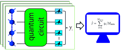
Figure 1: Schematic of our strategy. To learn the expectation value $\expectationvalue{X}_{\rho}$ of an observable $X$ in $\rho$ which is possibly a many-body state, we perform the projective measurement of the observable $Y$ on each sample. This measurement can be implemented by utilizing the quantum circuit $V$ to transform the eigenbasis of $Y$ into the computational basis and then performing the standard measurement in the computational basis. Repeating this procedure $M_{\textrm{min}}=\lceil(\Delta Y)^{2}/\epsilon\rceil$ times, we can obtain an estimate of $\expectationvalue{X}_{\rho}$ up to the desired precision $\epsilon$ by post-processing the outcomes $y_{i}$ via the sample mean estimator.

With the above analysis, we are ready to specify our strategy in what follows. To obtain $\expectationvalue{X}_{\rho}$, our strategy is to perform the projective measurement of $Y=\mathcal{T}(X)$ on each sample, which, after post-processing the outcomes via the sample mean estimator, can produce the same expectation value with $X$ but requires $M_{\textrm{min}}=\lceil(\Delta Y)^{2}/\epsilon\rceil$ samples for reaching the desired precision $\epsilon$. Note that the projective measurement of $Y$ typically belongs to the class of entangling measurements, because (some of) the $U_{g}$’s act on multiple subsystems for most of the symmetric structures of interest in physics. To implement this measurement, we can first apply the quantum circuit $V$ transforming the eigenbasis of $Y$ into the computational basis and then perform the standard measurement in the computational basis (see Fig. 1). So, the working principle of our strategy is to leverage quantum computational resources for reducing the number of samples required to its minimal value. Notably, as the projective measurement of $Y$ saturates the QCRB, our strategy, theoretically speaking, operates at the optimal sample efficiency allowed by quantum mechanics and therefore outperforms other methods from the perspective of sample complexity.

Illustrative application 1: translational symmetries. Let us now apply our strategy to the scenario that $\rho$ is an unknown state of $n$ qubits with the symmetric structures described by the translation group $G=\{T^{i},i=0,\cdots,2^{n}-1\}$. Here, $T$ is defined as $T\ket{j}=\ket{j+1}$ with the periodic boundary condition $\ket{2^{n}}=\ket{0}$, where $\ket{j}$, $j=0,\cdots,2^{n}-1$, denote the computational basis. Note that translational symmetries are ubiquitous in condensed-matter physics. The above scenario could arise, e.g., in quantum simulations of electrons in crystalline solids Bloch et al. (2012); Georgescu et al. (2014), for which Bloch’s theorem states that solutions to the Schrödinger equations in periodic potentials are Bloch states and hence respect translational symmetries.

To show the usefulness of our strategy, we calculate $(\Delta X)^{2}$ and $(\Delta Y)^{2}$, which are respectively proportional to the numbers of samples required in the commonly used approach and our strategy for obtaining $\expectationvalue{X}_{\rho}$ up to $\epsilon$. To this end, we write $\rho$ as $\rho=\sum_{j}p_{j}\ket{f_{j}}\bra{f_{j}}$, which follows from $[\rho,T]=0$. Here, $p_{j}\geq 0$ satisfies $\sum_{j}p_{j}=1$, and $\ket{f_{j}}=\sum_{k}e^{2\pi ijk/2^{n}}\ket{k}/{\sqrt{2^{n}}}$ denotes the Fourier basis which is the eigenbasis of $T$. Then, expressing $X$ as $X=\sum_{jk}X_{jk}\ket{f_{j}}\bra{f_{k}}$ with $X_{jk}=\bra{f_{j}}X\ket{f_{k}}$, we have $(\Delta X)^{2}=(\sum_{jk}p_{j}\absolutevalue{X_{jk}}^{2})-(\sum_{j}p_{j}X_{jj})^{2}$. Besides, using Eq. (4) and noting that $T\ket{f_{j}}=e^{-2\pi ij/2^{n}}\ket{f_{j}}$, we have $Y=\sum_{j}X_{jj}\ket{f_{j}}\bra{f_{j}}$, which further leads to $(\Delta Y)^{2}=(\sum_{j}p_{j}{X}_{jj}^{2})-(\sum_{j}p_{j}X_{jj})^{2}$. Hence, $(\Delta X)^{2}-(\Delta Y)^{2}=\sum_{j,k\neq j}p_{j}\absolutevalue{X_{jk}}^{2}$ contains exponentially many nonnegative terms. Roughly speaking, this indicates that our strategy allows for dramatically reducing sample complexity for countless choices of $X$. To clearly see this point, we take $X=\bigotimes_{l=1}^{n}(\sigma_{x}^{l}+\sigma_{z}^{l})$ as an example, where $\sigma_{\alpha}^{l}$, $\alpha=x,y,z$, are the Pauli matrices acting on the $l$-th qubit. The corresponding $Y$ can be found by exploiting this expression to calculate $X_{jj}$ SM . We have $2^{n}-1\leq(\Delta X)^{2}\leq 2^{n}$ but $0\leq(\Delta Y)^{2}\leq 1$ SM , demonstrating that the reduction allowed by our strategy can be exponential in $n$.

We point out that our strategy is efficiently implementable on a quantum computer in the scenario under consideration. Indeed, the eigenbasis of $Y$ is the Fourier basis, which implies that the quantum circuit $V$ is just the inverse quantum Fourier transform. That our strategy is efficiently implementable follows from the known result that the inverse quantum Fourier transform can be realized as a quantum circuit consisting of only $\mathcal{O}(n^{2})$ Hadamard gates and controlled phase shift gates Nielsen and Chuang (2010) (see also Ref. Griffiths and Niu (1996) for a semiclassical realization without using two-bit gates).

Illustrative application 2: permutational symmetries. Let us consider again $n$ qubits but in the state whose symmetric structures are described by the permutation group $G=\{P_{s},s\in S_{n}\}$. Here, $s$ labels a permutation in the symmetric group $S_{n}$ and $P_{s}$ is defined by $P_{s}\ket{\psi_{1}}\otimes\cdots\otimes\ket{\psi_{n}}=\ket{\psi_{s(1)}}\otimes\cdots\otimes\ket{\psi_{s(n)}}$. This scenario arises frequently in multipartite experiments Kiesel et al. (2007); Wieczorek et al. (2009); Prevedel et al. (2009), in which the states involved are typically invariant under permutations Tóth et al. (2010). For example, three well-known states of this type are Werner states Werner (1989), Dicke states Dicke (1954), and Greenberger–Horne–Zeilinger (GHZ) states Greenberger et al. (1989), which are key resources in quantum information processing Horodecki et al. (2009); Gühne and Tóth (2009). Below, motivated by the fact that Pauli measurements are widely used in multipartite experiments, we explore our strategy to reduce sample complexity in Pauli measurements.

We can express a generic Pauli observable as $X_{\bm{kl}}=\sigma_{x}^{k_{1}}\sigma_{z}^{l_{1}}\otimes\cdots\otimes\sigma_{x}^{k_{n}}\sigma_{z}^{l_{n}}(i)^{\bm{k}\cdot\bm{l}}$, where $\bm{k}=(k_{1},\cdots,k_{n})$ and $\bm{l}=(l_{1},\cdots,l_{n})$ are two vectors of binary numbers and $\bm{k}\cdot\bm{l}=\sum_{i=1}^{n}k_{i}l_{i}$ denotes the usual dot product. Note that, associated to each $X_{\bm{kl}}$, there is a symmetrized counterpart $Y_{\bm{kl}}=\mathcal{T}(X_{\bm{kl}})$. To illustrate the superiority of the projective measurement of $Y_{\bm{kl}}$ over the Pauli measurement of $X_{\bm{kl}}$, we evaluate $(\Delta X_{\bm{kl}})^{2}$ and $(\Delta Y_{\bm{kl}})^{2}$ on the GHZ state of $n$ qubits. Hereafter we assume for simplicity that $n$ is odd. It can be shown that $(\Delta X_{\bm{kl}})^{2}=1$ for any Pauli observable with $\absolutevalue{\bm{k}}\neq 0$ and $n$ SM . Here $\absolutevalue{\bm{k}}=\sum_{i=1}^{n}k_{i}$. By contrast, $(\Delta Y_{\bm{kl}})^{2}=1/\binom{n}{\absolutevalue{\bm{k}}}$ for the same Pauli observable SM . To clearly see the difference between $(\Delta X_{\bm{kl}})^{2}$ and $(\Delta Y_{\bm{kl}})^{2}$, we consider the Pauli measurements with $(1-\delta)\frac{n}{2}<\absolutevalue{\bm{k}}<(1+\delta)\frac{n}{2}$, referred to as the typical Pauli measurements for ease of language. Here, $0<\delta<1$ is fixed. We show that $(\Delta X)^{2}/(\Delta Y)^{2}\geq\sqrt{\frac{2}{n\pi(1-\delta^{2})}}\left[\frac{4}{(1-\delta)^{1-\delta}(1+\delta)^{1+\delta}}\right]^{\frac{n}{2}}$ for any typical Pauli measurement SM . Noting that $(1-\delta)^{1-\delta}(1+\delta)^{1+\delta}<4$ for $0<\delta<1$, we deduce that $(\Delta X)^{2}/(\Delta Y)^{2}$ is exponential in $n$. Besides, we show that the number of the typical Pauli measurements is $\geq 4^{n}(1-\frac{1}{n\delta^{2}})$ SM . Since the total number of Pauli measurements is $4^{n}$, this means that most of Pauli measurements are typical for a large $n$. Therefore, our strategy allows for exponentially reducing sample complexity for most of Pauli measurements when $n$ is large.

Notably, our strategy can be efficiently implemented on a quantum computer in the considered scenario, too. Indeed, as detailed in SM SM , the eigenbasis of $Y$ can be mapped into the computational basis via the quantum Schur transform followed by at most $\lceil\frac{n}{2}\rceil$ controlled gates. That our strategy is efficiently implementable follows from the known result that the quantum Schur transform can be realized as a quantum circuit of polynomial size Bacon et al. (2006).

Before concluding, we present a few remarks. We point out that the relations $\expectationvalue{Y}_{\rho}=\expectationvalue{X}_{\rho}$ and $(\Delta Y)^{2}\leq(\Delta X)^{2}$ hold as long as $\rho$ admits some symmetric structures described by a finite or compact Lie group. That is, our strategy is applicable to any such $\rho$, regardless of whether the foregoing assumption, i.e., nothing about $\rho$ except its symmetric structures is known, is satisfied or not. When this assumption is satisfied, our strategy allows for consuming the fewest samples to learn $\expectationvalue{X}_{\rho}$ up to the desired precision $\epsilon$. On the other hand, while the assumption is satisfied in numerous scenarios, there are also many scenarios in which we know other structures of $\rho$ besides its symmetric structures. For example, apart from translational symmetries, the state of a many-body system usually admits quasi-local structures, based on which some learning methods have been proposed Anshu et al. (2021); Rouzé and França (2021). As such, our strategy could be incorporated into existing methods as a basic building block for further reducing sample complexity via making best use of symmetric structures of states.

In conclusion, targeting at learning expectation values of observables, we have proposed an entangling-measurement-based strategy that can leverage quantum computational resources to dramatically reduce sample complexity. Our strategy, which is powered by the exploration of symmetric structures of states, is to infer the expectation value of an observable $X$ from the projective measurement of its symmetrized counterpart $Y=\mathcal{T}(X)$ rather than $X$ itself. This enables our strategy to operate at the optimal sample efficiency in a variety of contexts and thereby go beyond what can be achieved with local measurements.

To illustrate the significance of our strategy, we have applied it to two scenarios involving different kinds of symmetric structures of states, i.e., those described respectively by the translation and permutation groups, which are ubiquitous in condensed-matter physics and quantum many-body physics. In all the scenarios, we have shown that our strategy allows for yielding exponential reductions in sample complexity while merely consuming polynomial amounts of quantum computational resources.

The present Letter opens many interesting topics for future work, e.g., how to optimally take advantage of symmetric structures of states to simultaneously learn expectation values of multiple observables and further to extend the scope of discussions from expectation values of observables to other properties like various resource measures Zhang et al. (2018).

Supplemental Material

I Fundamentals of quantum metrology

Here we recall some fundamentals of quantum metrology, whose mathematical foundation is the quantum parameter estimation theory Helstrom (1976); Holevo (2011). The theory deals with the quantum parameter estimation problems, in which both the state in question and the quantity of interest are characterized by some unknown parameters. Specifically, the state in question can be a density matrix $\rho(\bm{\theta})$ characterized by $\mathfrak{p}$ unknown parameters $\bm{\theta}=(\theta_{1},\cdots,\theta_{\mathfrak{p}})$, and the quantity of interest could be a function of $\bm{\theta}$, denoted as $\beta(\bm{\theta})$. Given $M$ copies of $\rho(\bm{\theta})$, the task is to estimate the value of $\beta$ from the outcome of a measurement performed on $\rho(\bm{\theta})^{\otimes M}$. Any measurement can be described by a positive operator-valued measure $\Pi_{x}$ satisfying $\sum_{x}\Pi_{x}=\openone$, where $x$ labels the outcome of the measurement. Here, albeit written as a single discrete variable, $x$ could be continuous or multivariate. Any inference rule amounts to an estimator $\hat{\beta}(x)$, i.e., a map from the set of measurement outcomes to the set of possible values of $\beta$. The deviation of $\hat{\beta}(x)$ from $\beta$ is quantified by Braunstein and Caves (1994)

$$\delta\beta(x):=\frac{\hat{\beta}(x)}{\absolutevalue{d\expectationvalue{\hat{\beta}}/d\beta}}-\beta.$$ (I.0S.1)

Here, $\expectationvalue{\hat{\beta}}$ is the statistical average of $\hat{\beta}(x)$ over potential outcomes $x$,

$$\expectationvalue{\hat{\beta}}=\sum_{x}p_{x}({\bm{\theta}})\hat{\beta}(x),$$ (I.0S.2)

where $p_{x}({\bm{\theta}})=\tr[\Pi_{x}\rho(\bm{\theta})^{\otimes M}]$. $d\expectationvalue{\hat{\beta}}/d\beta$ in Eq. (I.0S.1) is used to remove the local difference in the “units” of the estimate $\hat{\beta}$ and the value $\beta$ Braunstein and Caves (1994). The estimation error is defined as Braunstein and Caves (1994)

$${\expectationvalue{(\delta\beta)^{2}}}=\sum_{x}p_{x}(\bm{\theta})[\delta\beta(x)]^{2},$$ (I.0S.3)

i.e., the statistical average of $[\delta\beta(x)]^{2}$ over potential outcomes $x$. A central result in the quantum parameter estimation theory is that $\expectationvalue{(\delta\beta)^{2}}$ is bounded from below as Helstrom (1976); Holevo (2011); Braunstein and Caves (1994),

$$\expectationvalue{(\delta\beta)^{2}}\geq\frac{\partial\beta[H(\bm{\theta})]^{-1}\partial\beta^{T}}{M},$$ (I.0S.4)

known as the quantum Cramér-Rao bound (QCRB). Here, as specified in the main text, $H(\theta)$ is the quantum Fisher information (QFI) matrix. The meaning of the QCRB is that quantum mechanics does not allow for estimating $\beta$ with arbitrarily high precision. Instead, the precision attainable in any strategy for estimating $\beta$ with the $M$ copies of $\rho(\bm{\theta})$ is fundamentally constrained by the QCRB, which represents the ultimate precision allowed by quantum mechanics Braunstein and Caves (1994); Zhang and Gong (2020); Zhang and Tong (2022). In particular, when $\hat{\beta}(x)$ is unbiased, i.e., $\expectationvalue{\hat{\beta}}=\beta$, there is $\delta\beta(x)=\hat{\beta}(x)-\expectationvalue{\hat{\beta}}$. Hence,

$$\expectationvalue{(\delta\beta)^{2}}=\textrm{Var}[\hat{\beta}],$$ (I.0S.5)

i.e., $\expectationvalue{(\delta\beta)^{2}}$ is simply the variance for an unbiased estimator. Inserting Eq. (I.0S.5) into Eq. (I.0S.4) gives Eq. (1) in the main text.

II Parameterization of symmetric states

Here we show how to characterize $\rho$ in terms of unknown parameters. To do this, we introduce a $\mathbb{C}^{*}$-algebra Curtis and Reiner (1962),

$$\mathcal{A}=\{A|[A,U_{g}]=0,\forall g\in G\},$$ (II.0S.6)

which is comprised of all the complex matrices commuting with $U_{g}$. Standard structure theorems for $\mathbb{C}^{*}$-algebras Curtis and Reiner (1962) imply that $\mathcal{A}$ has a unique representation of the form

$$\mathcal{A}\cong\bigoplus_{\alpha=1}^{s}\textrm{L}(\mathbb{C}^{n_{\alpha}})\otimes\openone_{d_{\alpha}},$$ (II.0S.7)

up to unitary equivalence. Here, $\alpha$ labels the $\alpha$-th irreducible representation of $G$ with dimension $d_{\alpha}$ and multiplicity $n_{\alpha}$, $\textrm{L}(\mathbb{C}^{n_{\alpha}})$ is the matrix algebra of all $n_{\alpha}\times n_{\alpha}$ complex matrices, and $\openone_{d_{\alpha}}$ denotes the $d_{\alpha}\times d_{\alpha}$ identity matrix. Using Eq. (II.0S.7) and noting that $\rho\in\mathcal{A}$, we can express $\rho$ as

$$\rho\cong\bigoplus_{\alpha=1}^{s}q_{\alpha}\rho_{\alpha}\otimes\frac{\openone_{d_{\alpha}}}{d_{\alpha}},$$ (II.0S.8)

where $q_{\alpha}\geq 0$ satisfies $\sum_{\alpha=1}^{s}q_{\alpha}=1$ and $\rho_{\alpha}$ denotes a density matrix in $\textrm{L}(\mathbb{C}^{n_{\alpha}})$. We can further expand $\rho_{\alpha}$ by the generators $\bm{\lambda}_{\alpha}=(\lambda_{\alpha,1},\cdots,\lambda_{\alpha,n_{\alpha}^{2}-1})$ of Lie algebra $\mathfrak{su}(n_{\alpha})$,

$$\rho_{\alpha}=\frac{\openone_{n_{\alpha}}}{n_{\alpha}}+\frac{1}{2}\bm{r}_{\alpha}\cdot\bm{\lambda}_{\alpha},$$ (II.0S.9)

where $\bm{r}_{\alpha}\in\mathbb{R}^{n_{\alpha}^{2}-1}$ is the generalized Bloch vector Kimura (2003). The generators satisfy

$$\lambda_{\alpha,i}^{\dagger}=\lambda_{\alpha,i},~{}~{}\tr\lambda_{\alpha,i}=0,~{}~{}\tr(\lambda_{\alpha,i}\lambda_{\alpha,j})=2\delta_{ij},$$ (II.0S.10)

and they are characterized by structure constants $f_{\alpha,ijk}$ (completely antisymmetric tensor) and $g_{\alpha,ijk}$ (completely symmetric tensor) as

$$[\lambda_{\alpha,i},\lambda_{\alpha,j}]=2i\sum_{k}f_{\alpha,ijk}\lambda_{\alpha,k},$$ (II.0S.11)

and

$$\{\lambda_{\alpha,i},\lambda_{\alpha,j}\}=4\delta_{ij}\frac{\openone_{n_{\alpha}}}{n_{\alpha}}+2\sum_{k}g_{\alpha,ijk}\lambda_{\alpha,k},$$ (II.0S.12)

where $\{\cdot,\cdot\}$ denotes the anticommutator. From Eqs. (II.0S.8) and (II.0S.9), it follows that $\rho$ can be characterized by the parameters $\bm{\theta}:=({\bm{q}},\bm{r}_{1},\cdots,\bm{r}_{s})$. Here, in view of the constraint that $\sum_{\alpha=1}^{s}q_{\alpha}=1$, we have chosen ${\bm{q}}:=(q_{1},\cdots,q_{s-1})$ as independent parameters without loss of generality.

III Proof of Eq. (3)

Here we present a proof of Eq. (3) in the main text. To derive $\partial\beta$ where $\beta=\expectationvalue{X}_{\rho}$, we make use of the equality

$$\expectationvalue{X}_{\rho}=\expectationvalue{Y}_{\rho},$$ (III.0S.13)

which follows from the normalization of the Haar measure $\int_{G}d\nu(g)=1$ not and $U_{g}\rho U_{g}^{\dagger}=\rho$. Besides, the translation-invariant property of the Haar measure implies that $Y\in\mathcal{A}$, which allows us to express $Y$ in the form

$$Y\cong\bigoplus_{\alpha=1}^{s}Y_{\alpha}\otimes\openone_{d_{\alpha}},$$ (III.0S.14)

with

$$Y_{\alpha}=a_{\alpha}\openone_{n_{\alpha}}+\bm{b}_{\alpha}\cdot\bm{\lambda}_{\alpha}.$$ (III.0S.15)

Here, $a_{\alpha}\in\mathbb{R}$ and $\bm{b}_{\alpha}\in\mathbb{R}^{n_{\alpha}^{2}-1}$ are constants, as $Y$ is uniquely determined by $X$ through Eq. (4) in the main text. Inserting Eqs. (II.0S.8), (II.0S.9), (III.0S.14), and (III.0S.15) into Eq. (III.0S.13) to get

$$\expectationvalue{X}_{\rho}=\sum_{\alpha=1}^{s}q_{\alpha}l_{\alpha}$$ (III.0S.16)

and then differentiating $\expectationvalue{X}_{\rho}$ with respect to $\bm{\theta}$, we have

$$\partial\beta=\left(\bm{l}-l_{s}\bm{e},q_{1}\bm{b}_{1},\cdots,q_{s}\bm{b}_{s}\right),$$ (III.0S.17)

where

$$l_{\alpha}=a_{\alpha}+\bm{b}_{\alpha}\bm{r}_{\alpha}^{T},~{}~{}\bm{l}=(l_{1},\cdots,l_{s-1}),$$ (III.0S.18)

and $\bm{e}$ is a $(s-1)$-dimensional vector with all components identical to one. In Sec. IV, we figure out the QFI matrix for $\rho(\bm{\theta})$,

$$H(\bm{\theta})=H({\bm{q}})\bigoplus\left[\bigoplus_{\alpha=1}^{s}H(\bm{r}_{\alpha})\right],$$ (III.0S.19)

with

$$H({\bm{q}})=\textrm{diag}(\frac{1}{q_{1}},\cdots,\frac{1}{q_{s-1}})+\frac{1}{q_{s}}\bm{e}^{T}\bm{e}$$ (III.0S.20)

and

$$H(\bm{r}_{\alpha})=q_{\alpha}[R_{\alpha}-\bm{r}_{\alpha}^{T}\bm{r}_{\alpha}+\frac{2}{n_{\alpha}}\openone_{n_{\alpha}^{2}-1}]^{-1}.$$ (III.0S.21)

Here, all $q_{\alpha}$’s are assumed temporarily to be strictly larger than zero, and $R_{\alpha}$ is a $(n_{\alpha}^{2}-1)\times(n_{\alpha}^{2}-1)$ symmetric matrix with its $jk$ element defined as

$$R_{\alpha,jk}=\sum_{i}r_{\alpha,i}g_{\alpha,ijk},$$ (III.0S.22)

where $r_{\alpha,i}$ denotes the $i$-th component of $\bm{r}_{\alpha}$. Using Eqs. (III.0S.17) and (III.0S.19), we figure out the left-hand side (LHS) of Eq. (3),

$$\partial\beta H(\bm{\theta})^{-1}\partial\beta^{T}=\left(\sum_{\alpha=1}^{s}q_{\alpha}l_{\alpha}^{2}\right)-\left(\sum_{\alpha=1}^{s}q_{\alpha}l_{\alpha}\right)^{2}$$

$$+\sum_{\alpha=1}^{s}q_{\alpha}\bm{b}_{\alpha}\left(R_{\alpha}-\bm{r}_{\alpha}^{T}\bm{r}_{\alpha}+\frac{2}{n_{\alpha}}\openone_{n_{\alpha}^{2}-1}\right)\bm{b}_{\alpha}^{T},$$ (III.0S.23)

where we have used the equality

$$[H({\bm{q}})]^{-1}=\textrm{diag}(q_{1},\cdots,q_{s-1})-{\bm{q}}^{T}{\bm{q}}.$$ (III.0S.24)

To figure out the right-hand side (RHS) of Eq. (3), we deduce from Eqs. (II.0S.8) and (III.0S.14) that

$$\expectationvalue{Y^{2}}_{\rho}=\sum_{\alpha=1}^{s}q_{\alpha}\tr(\rho_{\alpha}Y_{\alpha}^{2}).$$ (III.0S.25)

Then, using Eqs. (II.0S.9) and (III.0S.15) and noting that

$$\tr(\bm{b}_{\alpha}\cdot\bm{\lambda}_{\alpha}\bm{r}_{\alpha}\cdot\bm{\lambda}_{\alpha})=2\bm{b}_{\alpha}\bm{r}_{\alpha}^{T},$$ (III.0S.26)

$$\tr(\bm{b}_{\alpha}\cdot\bm{\lambda}_{\alpha}\bm{b}_{\alpha}\cdot\bm{\lambda}_{\alpha})=2\bm{b}_{\alpha}\bm{b}_{\alpha}^{T},$$ (III.0S.27)

$$\tr(\bm{b}_{\alpha}\cdot\bm{\lambda}_{\alpha}\bm{r}_{\alpha}\cdot\bm{\lambda}_{\alpha}\bm{b}_{\alpha}\cdot\bm{\lambda}_{\alpha})=2\bm{b}_{\alpha}R_{\alpha}\bm{b}_{\alpha}^{T},$$ (III.0S.28)

we have

$$\expectationvalue{Y^{2}}_{\rho}=\sum_{\alpha=1}^{s}q_{\alpha}\left(a_{\alpha}^{2}+2a_{\alpha}\bm{b}_{\alpha}\bm{r}_{\alpha}^{T}+\frac{2}{n_{\alpha}}\bm{b}_{\alpha}\bm{b}_{\alpha}^{T}+\bm{b}_{\alpha}R_{\alpha}\bm{b}_{\alpha}^{T}\right).$$

Using this equality and noting that $\expectationvalue{Y}_{\rho}=\sum_{\alpha=1}^{s}q_{\alpha}l_{\alpha}$, we obtain

$$(\Delta Y)^{2} = \sum_{\alpha=1}^{s}q_{\alpha}(a_{\alpha}^{2}+2a_{\alpha}\bm{b}_{\alpha}\bm{r}_{\alpha}^{T}+\frac{2}{n_{\alpha}}\bm{b}_{\alpha}\bm{b}_{\alpha}^{T}+$$ (III.0S.29)

$$\bm{b}_{\alpha}R_{\alpha}\bm{b}_{\alpha}^{T})-\left(\sum_{\alpha=1}^{s}q_{\alpha}l_{\alpha}\right)^{2}.$$

Rewriting Eq. (III.0S.29) by taking into account

$$a_{\alpha}^{2}+2a_{\alpha}\bm{b}_{\alpha}\bm{r}_{\alpha}^{T}=l_{\alpha}^{2}-\bm{b}_{\alpha}\bm{r}_{\alpha}^{T}\bm{r}_{\alpha}\bm{b}_{\alpha}^{T}$$ (III.0S.30)

and further comparing the resultant equation with Eq. (III), we arrive at Eq. (3),

$$\partial\beta H(\bm{\theta})^{-1}\partial\beta^{T}=(\Delta Y)^{2}.$$ (III.0S.31)

As the set of invertible matrices belonging to $\mathcal{A}$ is a dense subset of $\mathcal{A}$, Eq. (III.0S.31) also holds when one or more $q_{\alpha}$ approach zero.

IV Derivation of Eq. (III.0S.19)

Here we derive the QFI matrix for $\rho(\bm{\theta})$. To do this, we need to figure out the symmetric logarithmic derivatives (SLDs) associated with the unknown parameters $\bm{\theta}=({\bm{q}},\bm{r}_{1},\cdots,\bm{r}_{s})$. The SLD associated with $q_{\alpha}$, denoted by $L_{q_{\alpha}}$, is the Hermitian operator that satisfies

$$\partialderivative{\rho}{q_{\alpha}}=\rho\circ L_{q_{\alpha}},$$ (IV.0S.32)

where $\alpha\in\{1,\cdots,s-1\}$. Noting that the LHS of Eq. (IV.0S.32) reads

$$\partialderivative{\rho}{q_{\alpha}}\cong\rho_{\alpha}\otimes\frac{\openone_{d_{\alpha}}}{d_{\alpha}}-\rho_{s}\otimes\frac{\openone_{d_{s}}}{d_{s}},$$ (IV.0S.33)

we have

$$L_{q_{\alpha}}\cong\frac{1}{q_{\alpha}}\openone_{n_{\alpha}}\otimes\openone_{d_{\alpha}}-\frac{1}{q_{s}}\openone_{n_{s}}\otimes\openone_{d_{s}}.$$ (IV.0S.34)

Here, $\cong$ means these equalities are up to a unitary transformation. On the other hand, the SLD associated with $r_{\alpha,i}$, denoted by $L_{r_{\alpha,i}}$, is the Hermitian operator satisfying

$$\partialderivative{\rho}{r_{\alpha,i}}=\rho\circ L_{r_{\alpha,i}}.$$ (IV.0S.35)

To solve Eq. (IV.0S.35), we assume the following ansatz for $L_{r_{\alpha,i}}$,

$$L_{r_{\alpha,i}}\cong\left(w_{\alpha,i}\openone_{n_{\alpha}}+\bm{v}_{\alpha,i}\cdot\bm{\lambda}_{\alpha}\right)\otimes\openone_{d_{\alpha}},$$ (IV.0S.36)

where $w_{\alpha,i}\in\mathbb{R}$ and $\bm{v}_{\alpha,i}\in\mathbb{R}^{n_{\alpha}^{2}-1}$ are to be determined. Besides, it is easy to see that the LHS of Eq. (IV.0S.35) reads

$$\partialderivative{\rho}{r_{\alpha,i}}\cong\frac{1}{2}q_{\alpha}\lambda_{\alpha,i}\otimes\frac{\openone_{d_{\alpha}}}{d_{\alpha}}.$$ (IV.0S.37)

Substituting Eqs. (IV.0S.36) and (IV.0S.37) into Eq. (IV.0S.35), we have

$$\left(\frac{\openone_{n_{\alpha}}}{n_{\alpha}}+\frac{1}{2}\bm{r}_{\alpha}\cdot\bm{\lambda}_{\alpha}\right)\circ\left(w_{\alpha,i}\openone_{n_{\alpha}}+\bm{v}_{\alpha,i}\cdot\bm{\lambda}_{\alpha}\right)=\frac{1}{2}\lambda_{\alpha,i},$$

which may be viewed as an equation in terms of $w_{\alpha,i}$ and $\bm{v}_{\alpha,i}$. Solving Eq. (IV) by resorting to the defining properties of $\bm{\lambda}_{\alpha}$ [specified in Eqs. (II.0S.10), (II.0S.11), and (II.0S.12)], we have

$$w_{\alpha,i}=-\bm{v}_{\alpha,i}\bm{r}_{\alpha}^{T},$$ (IV.0S.39)

and

$$\bm{v}_{\alpha,i}=\bm{h}_{\alpha,i}\left[R_{\alpha}-\bm{r}_{\alpha}^{T}\bm{r}_{\alpha}+\frac{2}{n_{\alpha}}\openone_{n_{\alpha}^{2}-1}\right]^{-1}.$$ (IV.0S.40)

Here, $R_{\alpha}$ is defined in Eq. (III.0S.22), and $\bm{h}_{\alpha,i}$ is a $(n_{\alpha}^{2}-1)$-dimensional vector with its $i$-th component identical to one and all others being zero. By the way, we point out that in the case that $[R_{\alpha}-\bm{r}_{\alpha}^{T}\bm{r}_{\alpha}+\frac{2}{n_{\alpha}}\openone_{n_{\alpha}^{2}-1}]$ is singular, $[R_{\alpha}-\bm{r}_{\alpha}^{T}\bm{r}_{\alpha}+\frac{2}{n_{\alpha}}\openone_{n_{\alpha}^{2}-1}]^{-1}$is understood as the Moore–Penrose inverse of $[R_{\alpha}-\bm{r}_{\alpha}^{T}\bm{r}_{\alpha}+\frac{2}{n_{\alpha}}\openone_{n_{\alpha}^{2}-1}]$. It is easy to see that for three matrices $A$, $B$, and $C$, there are

$$A\circ B=B\circ A,~{}~{}~{}~{}\tr[A(B\circ C)]=\tr[(A\circ B)C].$$ (IV.0S.41)

Using these two equalities and Eqs. (IV.0S.34), (IV.0S.35), and (IV.0S.37), we have

$$\tr\left[\rho\left(L_{q_{\alpha}}\circ L_{r_{\beta,i}}\right)\right]$$ (IV.0S.42)

$$= \tr\left[\left(\rho\circ L_{r_{\beta,i}}\right)L_{q_{\alpha}}\right]$$

$$= \tr(\partialderivative{\rho}{r_{\beta,i}}L_{q_{\alpha}})$$

$$\cong \tr\left[\frac{1}{2}q_{\beta}\lambda_{\beta,i}\otimes\frac{\openone_{d_{\beta}}}{d_{\beta}}\left(\frac{1}{q_{\alpha}}\openone_{n_{\alpha}}\otimes\openone_{d_{\alpha}}-\frac{1}{q_{s}}\openone_{n_{s}}\otimes\openone_{d_{s}}\right)\right]$$

$$= 0.$$

Here, $\beta$ is a subscript and should be distinguished from the notation used in the main text. Using Eq. (IV.0S.36), we easily have

$$\tr\left[\rho\left(L_{r_{\alpha,i}}\circ L_{r_{\beta,j}}\right)\right]=0,$$ (IV.0S.43)

for $\alpha\neq\beta$. From Eqs. (IV.0S.42) and (IV.0S.43), we deduce that $H(\bm{\theta})$ can be expressed in the following block-diagonal form

$$H(\bm{\theta})=H({\bm{q}})\bigoplus\left[\bigoplus_{\alpha=1}^{s}H(\bm{r}_{\alpha})\right],$$ (IV.0S.44)

where $H({\bm{q}})$ is a $(s-1)\times(s-1)$ symmetric matrix with its $\alpha\beta$ element defined as

$$\left[H({\bm{q}})\right]_{\alpha\beta}=\tr[\rho(L_{q_{\alpha}}\circ L_{q_{\beta}})],$$ (IV.0S.45)

and $H(\bm{r}_{\alpha})$ is a $(n_{\alpha}^{2}-1)\times(n_{\alpha}^{2}-1)$ symmetric matrix with its $ij$ element defined as

$$\left[H(\bm{r}_{\alpha})\right]_{ij}=\tr[\rho\left(L_{r_{\alpha,i}}\circ L_{r_{\alpha,j}}\right)].$$ (IV.0S.46)

Inserting Eq. (IV.0S.34) into Eq. (IV.0S.45), we have, after simple algebra,

$$\left[H({\bm{q}})\right]_{\alpha\beta}=\delta_{\alpha\beta}\frac{1}{q_{\alpha}}+\frac{1}{q_{s}},$$ (IV.0S.47)

that is,

$$H({\bm{q}})=\textrm{diag}(\frac{1}{q_{1}},\cdots,\frac{1}{q_{s-1}})+\frac{1}{q_{s}}\bm{e}^{T}\bm{e}.$$ (IV.0S.48)

Substituting Eqs. (IV.0S.36), (IV.0S.37), (IV.0S.39), and (IV.0S.40) into Eq. (IV.0S.46) gives

$$\left[H(\bm{r}_{\alpha})\right]_{ij}$$ (IV.0S.49)

$$= \tr[\rho\left(L_{r_{\alpha,i}}\circ L_{r_{\alpha,j}}\right)]$$

$$= \tr[\left(\rho\circ L_{r_{\alpha,i}}\right)L_{r_{\alpha,j}}]$$

$$= \tr[\partialderivative{\rho}{r_{\alpha,i}}L_{r_{\alpha,j}}]$$

$$= \tr[\left(\frac{1}{2}q_{\alpha}\lambda_{\alpha,i}\otimes\frac{\openone_{d_{\alpha}}}{d_{\alpha}}\right)\left(w_{\alpha,j}\openone_{n_{\alpha}}+\bm{v}_{\alpha,j}\cdot\bm{\lambda}_{\alpha}\right)\otimes\openone_{d_{\alpha}}]$$

$$= q_{\alpha}\bm{h}_{\alpha,i}\bm{v}_{\alpha,j}^{T}$$

$$= q_{\alpha}\bm{h}_{\alpha,i}\left[R_{\alpha}-\bm{r}_{\alpha}^{T}\bm{r}_{\alpha}+\frac{2}{n_{\alpha}}\openone_{n_{\alpha}^{2}-1}\right]^{-1}\bm{h}_{\alpha,j}^{T}.$$

That is,

$$H(\bm{r}_{\alpha})=q_{\alpha}\left[R_{\alpha}-\bm{r}_{\alpha}^{T}\bm{r}_{\alpha}+\frac{2}{n_{\alpha}}\openone_{n_{\alpha}^{2}-1}\right]^{-1}.$$ (IV.0S.50)

Now, the QFI matrix for $\rho(\bm{\theta})$ is given by Eqs. (IV.0S.44) with Eq. (IV.0S.48) and (IV.0S.50).

V Details on application 1

Here we prove the two inequalities used in the main text,

$$2^{n}-1\leq(\Delta X)^{2}\leq 2^{n},$$ (V.0S.51)

and

$$0\leq(\Delta Y)^{2}\leq 1.$$ (V.0S.52)

To do this, we resort to the product representation of the Fourier basis Nielsen and Chuang (2010),

$$\ket{f_{j}}=\frac{\left(\ket{0}+e^{2\pi i0.j_{n}}\ket{1}\right)\cdots\left(\ket{0}+e^{2\pi i0.j_{1}\cdots j_{n}}\ket{1}\right)}{2^{n/2}},$$

where $0.j_{l}j_{l+1}\cdots j_{m}$ denotes the binary fraction $j_{l}/2+j_{l+1}/4+\cdots+j_{m}/2^{m-l+1}$. Using Eq. (V) to calculate $X_{jj}=\bra{f_{j}}X\ket{f_{j}}$ gives

$$X_{jj}=\cos(2\pi 0.j_{n})\cdots\cos(2\pi 0.j_{1}j_{2}\cdots j_{n}).$$ (V.0S.54)

Noting that $\absolutevalue{X_{jj}}\leq 1$ and $\rho=\sum_{j}p_{j}\ket{f_{j}}\bra{f_{j}}$, we have

$$\absolutevalue{\expectationvalue{X}_{\rho}}=\absolutevalue{\sum_{j}p_{j}X_{jj}}\leq\sum_{j}p_{j}\absolutevalue{X_{jj}}\leq\sum_{j}p_{j}=1.$$ (V.0S.55)

Besides, note that $X^{2}=2^{n}\openone\otimes\cdots\otimes\openone$ and therefore

$$\expectationvalue{X^{2}}_{\rho}=2^{n}.$$ (V.0S.56)

Then Eq. (V.0S.51) follows from Eqs. (V.0S.55) and (V.0S.56). On the other hand, noting that $Y=\sum_{j}X_{jj}\ket{f_{j}}\bra{f_{j}}$, we have

$$\absolutevalue{\expectationvalue{Y}_{\rho}}=\absolutevalue{\expectationvalue{X}_{\rho}}\leq 1,$$ (V.0S.57)

and

$$\expectationvalue{Y^{2}}_{\rho}=\sum_{j}p_{j}X_{jj}^{2}\leq 1.$$ (V.0S.58)

It is easy to see that Eq. (V.0S.52) follows from Eqs. (V.0S.57) and (V.0S.58).

VI Details on application 2

VI.1 Calculating $(\Delta X_{\bm{kl}})^{2}$ and $(\Delta Y_{\bm{kl}})^{2}$

Here we figure out the expressions of $(\Delta X_{\bm{kl}})^{2}$ and $(\Delta Y_{\bm{kl}})^{2}$. Note that

$$\sigma_{x}^{k_{1}}\sigma_{z}^{l_{1}}\otimes\cdots\otimes\sigma_{x}^{k_{n}}\sigma_{z}^{l_{n}}\ket{GHZ}=$$

$$\frac{1}{\sqrt{2}}\left[\ket{k_{1},\cdots,k_{n}}+(-1)^{\absolutevalue{\bm{l}}}\ket{1-k_{1},\cdots,1-k_{n}}\right],$$

with the $n$-qubit GHZ state $\ket{GHZ}=\left(\ket{0\cdots 0}+\ket{1\cdots 1}\right)/\sqrt{2}$ and $\absolutevalue{\bm{l}}=\sum_{i=1}^{n}l_{i}$. Using Eq. (VI.1) and

$$X_{\bm{kl}}=\sigma_{x}^{k_{1}}\sigma_{z}^{l_{1}}\otimes\cdots\otimes\sigma_{x}^{k_{n}}\sigma_{z}^{l_{n}}(i)^{\bm{k}\cdot\bm{l}},$$ (VI.1S.60)

we have

$$\bra{GHZ}X_{\bm{kl}}\ket{GHZ}=(i)^{\bm{k}\cdot\bm{l}}\frac{1+(-1)^{\absolutevalue{\bm{l}}}}{2}(\delta_{\bm{k},\bm{0}}+\delta_{\bm{k},\bm{1}}),$$

where $\delta_{\bm{k},\bm{0}}:=\delta_{k_{1},0}\cdots\delta_{k_{n},0}$ and $\delta_{\bm{k},\bm{1}}:=\delta_{k_{1},1}\cdots\delta_{k_{n},1}$. Hence,

$$\bra{GHZ}X_{\bm{kl}}\ket{GHZ}=$$

$$\begin{cases}1&\bm{k}=\bm{0}~{}~{}\textrm{and}~{}~{}\absolutevalue{\bm{l}}\in\textrm{even numbers},\\ (i)^{\absolutevalue{\bm{l}}}&\bm{k}=\bm{1}~{}~{}\textrm{and}~{}~{}\absolutevalue{\bm{l}}\in\textrm{even numbers},\\ 0&\textrm{otherwise}.\end{cases}$$ (VI.1S.62)

It follows from Eq. (VI.1) and $X_{\bm{kl}}^{2}=\openone_{2^{n}}$ that

$$(\Delta X_{\bm{kl}})^{2}=\begin{cases}0&\bm{k}=\bm{0},\bm{1}~{}~{}\textrm{and}~{}~{}\absolutevalue{\bm{l}}\in\textrm{even numbers},\\ 1&\textrm{otherwise}.\end{cases}$$

To calculate $(\Delta Y_{\bm{kl}})^{2}$, we resort to the defining properties of $P_{s}$,

$$P_{s}\ket{\psi_{1}}\otimes\cdots\otimes\ket{\psi_{n}}=\ket{\psi_{s(1)}}\otimes\cdots\otimes\ket{\psi_{s(n)}}$$ (VI.1S.64)

and

$$P_{s}A_{1}\otimes\cdots\otimes A_{n}P_{s}^{\dagger}=A_{s(1)}\otimes\cdots\otimes A_{s(n)},$$ (VI.1S.65)

which, in conjunction with the rearrangement theorem, lead to

$$P_{s}\ket{GHZ}=\ket{GHZ},~{}~{}P_{s}Y_{\bm{kl}}=Y_{\bm{kl}}P_{s}.$$ (VI.1S.66)

Using Eq. (VI.1S.66) and

$$Y_{\bm{kl}}=\frac{1}{n!}\sum_{s\in S_{n}}\sigma_{x}^{k_{s(1)}}\sigma_{z}^{l_{s(1)}}\otimes\cdots\otimes\sigma_{x}^{k_{s(n)}}\sigma_{z}^{l_{s(n)}}(i)^{\bm{k}\cdot\bm{l}},$$

we have

$$\bra{GHZ}Y_{\bm{kl}}^{2}\ket{GHZ} = \frac{1}{n!}\sum_{s\in S_{n}}\bra{GHZ}\sigma_{x}^{k_{s(1)}}\sigma_{z}^{l_{s(1)}}\otimes\cdots\otimes\sigma_{x}^{k_{s(n)}}\sigma_{z}^{l_{s(n)}}(i)^{\bm{k}\cdot\bm{l}}Y_{\bm{kl}}\ket{GHZ}$$ (VI.1S.68)

$$= \frac{1}{n!}\sum_{s\in S_{n}}\bra{GHZ}P_{s}^{\dagger}\sigma_{x}^{k_{s(1)}}\sigma_{z}^{l_{s(1)}}\otimes\cdots\otimes\sigma_{x}^{k_{s(n)}}\sigma_{z}^{l_{s(n)}}(i)^{\bm{k}\cdot\bm{l}}Y_{\bm{kl}}P_{s}\ket{GHZ}$$

$$= \frac{1}{n!}\sum_{s\in S_{n}}\bra{GHZ}P_{s}^{\dagger}\sigma_{x}^{k_{s(1)}}\sigma_{z}^{l_{s(1)}}\otimes\cdots\otimes\sigma_{x}^{k_{s(n)}}\sigma_{z}^{l_{s(n)}}(i)^{\bm{k}\cdot\bm{l}}P_{s}Y_{\bm{kl}}\ket{GHZ}$$

$$= \frac{1}{n!}\sum_{s\in S_{n}}\bra{GHZ}\sigma_{x}^{k_{1}}\sigma_{z}^{l_{1}}\otimes\cdots\otimes\sigma_{x}^{k_{n}}\sigma_{z}^{l_{n}}(i)^{\bm{k}\cdot\bm{l}}Y_{\bm{kl}}\ket{GHZ}$$

$$= \bra{GHZ}\sigma_{x}^{k_{1}}\sigma_{z}^{l_{1}}\otimes\cdots\otimes\sigma_{x}^{k_{n}}\sigma_{z}^{l_{n}}(i)^{\bm{k}\cdot\bm{l}}Y_{\bm{kl}}\ket{GHZ}$$

$$= \frac{1}{n!}\sum_{s\in S_{n}}\bra{GHZ}\sigma_{x}^{k_{1}}\sigma_{z}^{l_{1}}\sigma_{x}^{k_{s(1)}}\sigma_{z}^{l_{s(1)}}\otimes\cdots\otimes\sigma_{x}^{k_{n}}\sigma_{z}^{l_{n}}\sigma_{x}^{k_{s(n)}}\sigma_{z}^{l_{s(n)}}(-1)^{\bm{k}\cdot\bm{l}}\ket{GHZ}$$

$$= \frac{1}{n!}\sum_{s\in S_{n}}\bra{GHZ}\sigma_{x}^{k_{1}+k_{s(1)}}\sigma_{z}^{l_{1}+l_{s(1)}}\otimes\cdots\otimes\sigma_{x}^{k_{n}+k_{s(n)}}\sigma_{z}^{l_{n}+l_{s(n)}}(-1)^{(\bm{k}+\bm{k}_{s})\cdot\bm{l}}\ket{GHZ}$$

$$= \frac{1}{n!}\sum_{s\in S_{n}}(-1)^{(\bm{k}+\bm{k}_{s})\cdot\bm{l}}\frac{1+(-1)^{\absolutevalue{\bm{l}+\bm{l}_{s}}}}{2}(\delta_{\bm{k}\oplus\bm{k}_{s},\bm{0}}+\delta_{\bm{k}\oplus\bm{k}_{s},\bm{1}}),$$

where $\bm{k}_{s}=(k_{s(1)},\cdots,k_{s(n)})$, $\bm{l}_{s}=(l_{s(1)},\cdots,l_{s(n)})$, and $\oplus$ denotes addition modulo $2$, that is, $\bm{k}\oplus\bm{k}_{s}=(k_{1}+k_{s(1)},\cdots,k_{n}+k_{s(n)})$ (mod $2$). Noting that $\absolutevalue{\bm{l}+\bm{l}_{s}}=\sum_{i=1}^{n}l_{i}+l_{s(i)}=2\absolutevalue{\bm{l}}$, we have $[1+(-1)^{\absolutevalue{\bm{l}+\bm{l}_{s}}}]/{2}=1$. Moreover, assuming that $n$ is odd, we have $\delta_{\bm{k}\oplus\bm{k}_{s},\bm{1}}=0$. So, the only nonzero terms in the summation of Eq. (VI.1S.68) are those such that $\bm{k}=\bm{k}_{s}$. The number of such terms is $\absolutevalue{\bm{k}}!(n-\absolutevalue{\bm{k}})!$. Besides, $(-1)^{(\bm{k}+\bm{k}_{s})\cdot\bm{l}}=1$ when $\bm{k}=\bm{k}_{s}$. We have

$$\bra{GHZ}Y_{\bm{kl}}^{2}\ket{GHZ}=1/\binom{n}{\absolutevalue{\bm{k}}}.$$ (VI.1S.69)

Noting that $\bra{GHZ}Y_{\bm{kl}}\ket{GHZ}=\bra{GHZ}X_{\bm{kl}}\ket{GHZ}$ and using Eqs. (VI.1) and (VI.1S.69), we arrive at the expression of $(\Delta Y_{\bm{kl}})^{2}$:

$$(\Delta Y_{\bm{kl}})^{2}=\begin{cases}0&\bm{k}=\bm{0},\bm{1}~{}~{}\textrm{and}~{}~{}\absolutevalue{\bm{l}}\in\textrm{even numbers},\\ 1/\binom{n}{\absolutevalue{\bm{k}}}&\textrm{otherwise}.\end{cases}$$

VI.2 Lower bound on $(\Delta X)^{2}/(\Delta Y)^{2}$ for typical Pauli measurements

Here we figure out the lower bound on $(\Delta X)^{2}/(\Delta Y)^{2}$ for typical Pauli measurements. Using the Stirling’s approximation

$$n!\approx\sqrt{2\pi n}\left(\frac{n}{e}\right)^{n}$$ (VI.2S.71)

and noting that

$$(1-\delta)\frac{n}{2}<\absolutevalue{\bm{k}}<(1+\delta)\frac{n}{2},$$ (VI.2S.72)

we have

$${(\Delta X)^{2}}/{(\Delta Y)^{2}} = \binom{n}{\absolutevalue{\bm{k}}}$$ (VI.2S.73)

$$\geq \binom{n}{(1-\delta)\frac{n}{2}}$$

$$= \frac{n!}{\left[(1-\delta)\frac{n}{2}\right]!\left[(1+\delta)\frac{n}{2}\right]!}$$

$$\approx \frac{\sqrt{2\pi n}\left(\frac{n}{e}\right)^{n}}{\sqrt{2\pi(1-\delta)\frac{n}{2}}\left(\frac{(1-\delta)\frac{n}{2}}{e}\right)^{(1-\delta)\frac{n}{2}}\sqrt{2\pi(1+\delta)\frac{n}{2}}\left(\frac{(1+\delta)\frac{n}{2}}{e}\right)^{(1+\delta)\frac{n}{2}}}$$

$$= \sqrt{\frac{2}{n\pi(1-\delta^{2})}}\left[\frac{4}{(1-\delta)^{1-\delta}(1+\delta)^{1+\delta}}\right]^{\frac{n}{2}}.$$

Here we have assumed for simplicity that $(1-\delta)\frac{n}{2}$ is an integer. The above proof can be made more rigorous by replacing the Stirling’s approximation with the inequalities $\sqrt{2\pi n}\left(\frac{n}{e}\right)^{n}e^{\frac{1}{12n+1}}\leq n!\leq\sqrt{2\pi n}\left(\frac{n}{e}\right)^{n}e^{\frac{1}{12n}}$ which hold for $n\geq 1$.

VI.3 Lower bound on the number of typical Pauli measurements

Here we find a lower bound on the number of typical Pauli measurements. To do this, we interpret all $k_{i}$’s as independent and identically distributed binary random variables taking on two values $0$ and $1$ with equal probabilities $1/2$. Then, all the bit strings $\bm{k}=(k_{1},\cdots,k_{n})$ are with equal probabilities $1/2^{n}$. Using the Chebyshev’s inequality Mitzenmacher and Upfal (2005) and noting that $\textrm{Var}[\absolutevalue{\bm{k}}]=\textrm{Var}[k_{1}+\cdots+k_{n}]=n/4$, we can bound from below the number of the bit strings with $(1-\delta)\frac{n}{2}<\absolutevalue{\bm{k}}<(1+\delta)\frac{n}{2}$ as

$$N = 2^{n}\textrm{Pr}\left((1-\delta)\frac{n}{2}<\absolutevalue{\bm{k}}<(1+\delta)\frac{n}{2}\right)$$ (VI.3S.74)

$$= 2^{n}\left[1-\textrm{Pr}\left(\absolutevalue{\absolutevalue{\bm{k}}-\frac{n}{2}}\geq\frac{n\delta}{2}\right)\right]$$

$$\geq 2^{n}\left[1-\frac{\textrm{Var}[\absolutevalue{\bm{k}}]}{\left(\frac{n\delta}{2}\right)^{2}}\right]$$

$$= 2^{n}\left(1-\frac{1}{n\delta^{2}}\right),$$

where $\textrm{Pr}\left((1-\delta)\frac{n}{2}<\absolutevalue{\bm{k}}<(1+\delta)\frac{n}{2}\right)$ stands for the probability that a bit string $\bm{k}$ is with $(1-\delta)\frac{n}{2}<\absolutevalue{\bm{k}}<(1+\delta)\frac{n}{2}$, and similarly for the notation $\textrm{Pr}\left(\absolutevalue{\absolutevalue{\bm{k}}-\frac{n}{2}}\geq\frac{n\delta}{2}\right)$. The number of typical Pauli measurements is

$$2^{n}N\geq 4^{n}\left(1-\frac{1}{n\delta^{2}}\right),$$ (VI.3S.75)

which follows from the fact that there are $2^{n}$ different $\bm{l}$ for each $\bm{k}$.

VI.4 Discussion on the implementation of $V$

Here we explain why the quantum circuit $V$ can be efficiently realized as a quantum circuit. According to the Schur–Weyl duality Weyl (1950), the Hilbert space $(\mathbb{C}^{2})^{\otimes n}$ of $n$ qubits can be decomposed into a direct sum of tensor products,

$$(\mathbb{C}^{2})^{\otimes n}\cong\bigoplus_{j=j_{\textrm{min}}}^{j_{\textrm{max}}}\mathbb{C}^{2j+1}\otimes\mathbb{C}^{d_{n,j}},$$ (VI.4S.76)

where $\mathbb{C}^{2j+1}$ and $\mathbb{C}^{d_{n,j}}$ are irreducible representations of $U(2)$ and $S_{n}$, respectively. $j$ labels the eigen-subspace of the total squared angular momentum with eigenvalue $j(j+1)$, where $j=j_{\textrm{min}}$, $j_{\textrm{min}}+1$, $\cdots$, $j_{\textrm{max}}$ with $j_{\textrm{max}}=n/2$ and $j_{\textrm{min}}=0$, $1/2$ for even and odd $n$, respectively. The decomposition (VI.4S.76) corresponds to a basis for $(\mathbb{C}^{2})^{\otimes n}$, $\ket{\Psi_{j,q,p}}$, known as the Schur basis Bacon et al. (2006), where $j$ labels the subspaces $\mathbb{C}^{2j+1}\otimes\mathbb{C}^{d_{n,j}}$, and $q$ and $p$ label bases for $\mathbb{C}^{2j+1}$ and $\mathbb{C}^{d_{n,j}}$, respectively. The Schur transform, denoted as $U_{\textrm{Sch}}$ hereafter, is defined as the unitary operator mapping the Schur basis into the computational basis,

$$U_{\textrm{Sch}}\ket{\Psi_{j,q,p}}=\ket{j,q,p}.$$ (VI.4S.77)

Here, $\ket{j,q,p}$ stands for the computational basis, with $j,q,p$ expressed as bit strings. A central result of Ref. Bacon et al. (2006) is that $U_{\textrm{Sch}}$ can be realized as a quantum circuit of polynomial size.

Without loss of generality, we can express $X$ in the form

$$X=\sum_{j,j^{\prime}}\sum_{q,q^{\prime}}\sum_{p,p^{\prime}}X_{jqp;j^{\prime}q^{\prime}p^{\prime}}\ket{\Psi_{j,q,p}}\bra{\Psi_{j^{\prime},q^{\prime},p^{\prime}}},$$ (VI.4S.78)

where

$$X_{jqp;j^{\prime}q^{\prime}p^{\prime}}=\bra{\Psi_{j,q,p}}X\ket{\Psi_{j^{\prime},q^{\prime},p^{\prime}}}.$$ (VI.4S.79)

Moreover, noting that $\rho$ and $Y$ belong to $\mathcal{A}\cong\bigoplus_{j=j_{\textrm{min}}}^{j_{\textrm{max}}}\textrm{L}(\mathbb{C}^{2j+1})\otimes\openone_{d_{n,j}}$, we can express $\rho$ and $Y$ in the form

$$\rho=\sum_{j}\sum_{q,q^{\prime}}\sum_{p}p_{j}(\rho_{j})_{qq^{\prime}}\ket{\Psi_{j,q,p}}\bra{\Psi_{j,q^{\prime},p}}$$ (VI.4S.80)

and

$$Y=\sum_{j}\sum_{q,q^{\prime}}\sum_{p}(Y_{j})_{qq^{\prime}}\ket{\Psi_{j,q,p}}\bra{\Psi_{j,q^{\prime},p}},$$ (VI.4S.81)

where $p_{j}\geq 0$ satisfies $\sum_{j}p_{j}=1$, $\rho_{j}$ is a density matrix, and $Y_{j}$ is a Hermitian matrix. To find the connection between $X$ and $Y$, we make use of the equality $\expectationvalue{X}_{\rho}=\expectationvalue{Y}_{\rho}$, which leads to

$$({Y}_{j})_{qq^{\prime}}=\frac{1}{d_{n,j}}\sum_{p}X_{jqp;jq^{\prime}p}.$$ (VI.4S.82)

It follows from Eqs. (VI.4S.77) and (VI.4S.81) that

$$U_{\textrm{Sch}}YU_{\textrm{Sch}}^{\dagger}=\sum_{j}\sum_{q,q^{\prime}}\sum_{p}(Y_{j})_{qq^{\prime}}\ket{{j,q,p}}\bra{{j,q^{\prime},p}}$$

$$=\sum_{j}\ket{j}\bra{j}\otimes\left(\sum_{q,q^{\prime}}(Y_{j})_{qq^{\prime}}\ket{q}\bra{q^{\prime}}\right)\otimes\openone_{d_{n,j}}.$$

Let the eigendecomposition of $Y_{j}$ be

$$Y_{j}=U_{j}D_{j}U_{j}^{\dagger},$$ (VI.4S.84)

where $U_{j}$ denotes a unitary matrix and $D_{j}$ is a diagonal matrix with real entries. We then define $V$ to be of the form

$$V=V_{j_{\textrm{min}}}\cdots V_{j_{\textrm{max}}}U_{\textrm{Sch}},$$ (VI.4S.85)

where

$$V_{j}=\ket{j}\bra{j}\otimes U_{j}^{\dagger}+\sum_{j^{\prime}\neq j}\ket{j^{\prime}}\bra{j^{\prime}}\otimes\openone_{2j+1}$$ (VI.4S.86)

is a controlled gate. It is easy to see that the $V$ thus defined transforms the eigenbasis of $Y$ into the computational basis $\ket{j,q,p}$. As each $V_{j}$ is a unitary matrix of polynomial size, $V$ can be realized as a quantum circuit of polynomial size.

References

• Biamonte et al. (2017) J. Biamonte, P. Wittek, N. Pancotti, P. Rebentrost, N. Wiebe,  and S. Lloyd, “Quantum machine learning,” Nature 549, 195 (2017).
• McArdle et al. (2020) S. McArdle, S. Endo, A. Aspuru-Guzik, S. C. Benjamin,  and X. Yuan, “Quantum computational chemistry,” Rev. Mod. Phys. 92, 015003 (2020).
• Cerezo et al. (2021) M. Cerezo, A. Arrasmith, R. Babbush, S. C. Benjamin, S. Endo, K. Fujii, J. R. McClean, K. Mitarai, X. Yuan, L. Cincio,  and P. J. Coles, “Variational quantum algorithms,” Nat. Rev. Phys. 3, 625 (2021).
• Tilly et al. (2022) J. Tilly, H. Chen, S. Cao, D. Picozzi, K. Setia, Y. Li, E. Grant, L. Wossnig, I. Rungger, G. H. Booth,  and J. Tennyson, “The variational quantum eigensolver: A review of methods and best practices,” Phys. Rep. 986, 1 (2022).
• Preskill (2018) J. Preskill, “Quantum computing in the NISQ era and beyond,” Quantum 2, 79 (2018).
• Gross et al. (2010) D. Gross, Y.-K. Liu, S. T. Flammia, S. Becker,  and J. Eisert, “Quantum state tomography via compressed sensing,” Phys. Rev. Lett. 105, 150401 (2010).
• Liu et al. (2012) W.-T. Liu, T. Zhang, J.-Y. Liu, P.-X. Chen,  and J.-M. Yuan, “Experimental quantum state tomography via compressed sampling,” Phys. Rev. Lett. 108, 170403 (2012).
• Cramer et al. (2010) M. Cramer, M. B. Plenio, S. T. Flammia, R. Somma, D. Gross, S. D. Bartlett, O. Landon-Cardinal, D. Poulin,  and Y.-K. Liu, “Efficient quantum state tomography,” Nat. Commun. 1, 149 (2010).
• Baumgratz et al. (2013) T. Baumgratz, D. Gross, M. Cramer,  and M. B. Plenio, “Scalable reconstruction of density matrices,” Phys. Rev. Lett. 111, 020401 (2013).
• Anshu et al. (2021) A. Anshu, S. Arunachalam, T. Kuwahara,  and M. Soleimanifar, “Sample-efficient learning of interacting quantum systems,” Nat. Phys. 17, 931 (2021).
• Rouzé and França (2021) C. Rouzé and D. S. França, “Learning quantum many-body systems from a few copies,” arXiv:2107.03333  (2021).
• Mahler et al. (2013) D. H. Mahler, L. A. Rozema, A. Darabi, C. Ferrie, R. Blume-Kohout,  and A. M. Steinberg, “Adaptive quantum state tomography improves accuracy quadratically,” Phys. Rev. Lett. 111, 183601 (2013).
• Qi et al. (2017) B. Qi, Z. Hou, Y. Wang, D. Dong, H.-S. Zhong, L. Li, G.-Y. Xiang, H. M. Wiseman, C.-F. Li,  and G.-C. Guo, “Adaptive quantum state tomography via linear regression estimation: Theory and two-qubit experiment,” npj Quant. Inf. 3, 19 (2017).
• Ferrie (2014) C. Ferrie, “Self-guided quantum tomography,” Phys. Rev. Lett. 113, 190404 (2014).
• Rambach et al. (2021) M. Rambach, M. Qaryan, M. Kewming, C. Ferrie, A. G. White,  and J. Romero, “Robust and efficient high-dimensional quantum state tomography,” Phys. Rev. Lett. 126, 100402 (2021).
• Aaronson (2018) S. Aaronson, “Shadow tomography of quantum states,” in Proceedings of the 50th Annual ACM SIGACT Symposium on Theory of Computing (ACM, 2018) pp. 325–338.
• Huang et al. (2020) H.-Y. Huang, R. Kueng,  and J. Preskill, “Predicting many properties of a quantum system from very few measurements,” Nat. Phys. 16, 1050 (2020).
• Peres and Wootters (1991) A. Peres and W. K. Wootters, “Optimal detection of quantum information,” Phys. Rev. Lett. 66, 1119 (1991).
• Gisin and Popescu (1999) N. Gisin and S. Popescu, “Spin flips and quantum information for antiparallel spins,” Phys. Rev. Lett. 83, 432–435 (1999).
• et al. (2022a) H.-Y. Huang et al., “Quantum advantage in learning from experiments,” Science 376, 1182 (2022a).
• Aharonov et al. (2022) D. Aharonov, J. Cotler,  and X.-L. Qi, “Quantum algorithmic measurement,” Nat. Commun. 13, 887 (2022).
• Miguel-Ramiro et al. (2022) J. Miguel-Ramiro, F. Riera-Sàbat,  and W. Dür, “Collective operations can exponentially enhance quantum state verification,” Phys. Rev. Lett. 129, 190504 (2022).
• Larocca et al. (2022) M. Larocca, F. Sauvage, F. M. Sbahi, G. Verdon, P. J. Coles,  and M. Cerezo, “Group-invariant quantum machine learning,” PRX Quantum 3, 030341 (2022).
• et al. (2022b) K. Bharti et al., “Noisy intermediate-scale quantum algorithms,” Rev. Mod. Phys. 94, 015004 (2022b).
• Tang et al. (2020) J.-F. Tang, Z. Hou, J. Shang, H. Zhu, G.-Y. Xiang, C.-F. Li,  and G.-C. Guo, “Experimental optimal orienteering via parallel and antiparallel spins,” Phys. Rev. Lett. 124, 060502 (2020).
• Huang et al. (2022) C.-X. Huang, X.-M. Hu, Y. Guo, C. Zhang, B.-H. Liu, Y.-F. Huang, C.-F. Li, G.-C. Guo, N. Gisin, C. Branciard,  and A. Tavakoli, “Entanglement swapping and quantum correlations via symmetric joint measurements,” Phys. Rev. Lett. 129, 030502 (2022).
• Conlon et al. (2023) L. O. Conlon, T. Vogl, C. D. Marciniak, I. Pogorelov, S. K. Yung, F. Eilenberger, D. W. Berry, F. S. Santana, R. Blatt, T. Monz, P. K. Lam,  and S. M. Assad, “Approaching optimal entangling collective measurements on quantum computing platforms,” Nat. Phys.  (2023), 10.1038/s41567-022-01875-7.
• Tóth et al. (2010) G. Tóth, W. Wieczorek, D. Gross, R. Krischek, C. Schwemmer,  and H. Weinfurter, “Permutationally Invariant Quantum Tomography,” Phys. Rev. Lett. 105, 250403 (2010).
• Helstrom (1976) C. W. Helstrom, Quantum Detection and Estimation Theory (Academic, New York, 1976).
• Holevo (2011) A. S. Holevo, Probabilistic and Statistical Aspects of Quantum Theory (Edizioni della Normale, Pisa, Italy, 2011).
• Braunstein and Caves (1994) S. L. Braunstein and C. M. Caves, “Statistical distance and the geometry of quantum states,” Phys. Rev. Lett. 72, 3439 (1994).
• Zhang and Gong (2020) D.-J. Zhang and J. Gong, “Dissipative adiabatic measurements: Beating the quantum Cramér-Rao bound,” Phys. Rev. Research 2, 023418 (2020).
• Zhang and Tong (2022) D.-J. Zhang and D. M. Tong, “Approaching Heisenberg-scalable thermometry with built-in robustness against noise,” npj Quant. Inf. 8, 81 (2022).
• (34) See Supplemental Material at [URL will be inserted by publisher] for some fundamentals of quantum metrology, the parameterization of $\rho$, and the proofs of miscellaneous equations used here.
• Halmos (1950) P. R. Halmos, Measure Theory (New York: Springer-Verlag, 1950).
• Bloch et al. (2012) I. Bloch, J. Dalibard,  and S. Nascimbène, “Quantum simulations with ultracold quantum gases,” Nat. Phys. 8, 267 (2012).
• Georgescu et al. (2014) I. M. Georgescu, S. Ashhab,  and F. Nori, “Quantum simulation,” Rev. Mod. Phys. 86, 153–185 (2014).
• Nielsen and Chuang (2010) M. A. Nielsen and I. L. Chuang, Quantum Computation and Quantum Information (Cambridge University Press, Cambridge, England, 2010).
• Griffiths and Niu (1996) R. B. Griffiths and C.-S. Niu, “Semiclassical fourier transform for quantum computation,” Phys. Rev. Lett. 76, 3228 (1996).
• Kiesel et al. (2007) N. Kiesel, C. Schmid, G. Tóth, E. Solano,  and H. Weinfurter, “Experimental Observation of Four-Photon Entangled Dicke State with High Fidelity,” Phys. Rev. Lett. 98, 063604 (2007).
• Wieczorek et al. (2009) W. Wieczorek, R. Krischek, N. Kiesel, P. Michelberger, G. Tóth,  and H. Weinfurter, “Experimental Entanglement of a Six-Photon Symmetric Dicke State,” Phys. Rev. Lett. 103, 020504 (2009).
• Prevedel et al. (2009) R. Prevedel, G. Cronenberg, M. S. Tame, M. Paternostro, P. Walther, M. S. Kim,  and A. Zeilinger, “Experimental Realization of Dicke States of up to Six Qubits for Multiparty Quantum Networking,” Phys. Rev. Lett. 103, 020503 (2009).
• Werner (1989) R. F. Werner, “Quantum states with Einstein-Podolsky-Rosen correlations admitting a hidden-variable model,” Phys. Rev. A 40, 4277 (1989).
• Dicke (1954) R. H. Dicke, “Coherence in spontaneous radiation processes,” Phys. Rev. 93, 99 (1954).
• Greenberger et al. (1989) D. M. Greenberger, M. A. Horne,  and A. Zeilinger, Bell’s Theorem, Quantum Theory, and Conceptions of the Universe, edited by M. Kafatos (Kluwer Academics, Dordrecht, The Netherlands, 1989).
• Horodecki et al. (2009) R. Horodecki, P. Horodecki, M. Horodecki,  and K. Horodecki, “Quantum entanglement,” Rev. Mod. Phys. 81, 865 (2009).
• Gühne and Tóth (2009) O. Gühne and G. Tóth, “Entanglement detection,” Phys. Rep. 474, 1 (2009).
• Bacon et al. (2006) D. Bacon, I. L. Chuang,  and A. W. Harrow, “Efficient Quantum Circuits for Schur and Clebsch-Gordan Transforms,” Phys. Rev. Lett. 97, 170502 (2006).
• Zhang et al. (2018) D.-J. Zhang, C. L. Liu, X.-D. Yu,  and D. M. Tong, “Estimating Coherence Measures from Limited Experimental Data Available,” Phys. Rev. Lett. 120, 170501 (2018).
• Curtis and Reiner (1962) C. W. Curtis and I. Reiner, Representation Theory of Finite Groups and Associative Algebras (Wiley, New York, 1962).
• Kimura (2003) G. Kimura, “The Bloch vector for $N$-level systems,” Phys. Lett. A 314, 339 (2003).
• (52) The normalized Haar measure exists if $G$ is a finite or compact Lie group. Notably, most of symmetries of interest in physics fall into these two categories.
• Mitzenmacher and Upfal (2005) M. Mitzenmacher and E. Upfal, Probability and Computing (Cambridge University Press, Cambridge, UK, 2005).
• Weyl (1950) H. Weyl, The Theory of Groups and Quantum Mechanics (Dover Publications, Inc., New York, 1950).