Beyond scalar quasi-arithmetic means: Quasi-arithmetic averages and quasi-arithmetic mixtures in information geometry

Abstract

We generalize quasi-arithmetic means beyond scalars by considering continuously invertible gradient maps of strictly convex Legendre type real-valued functions. Gradient maps of strictly convex Legendre type functions are strictly comonotone and admits a global inverse, thus generalizing the notion of strictly mononotone and differentiable functions used to define scalar quasi-arithmetic means. Furthermore, the Legendre transformation gives rise to pairs of dual quasi-arithmetic averages via the convex duality. We study both the invariance and equivariance properties under affine transformations of quasi-arithmetic averages via the lens of dually flat spaces of information geometry. We show how these quasi-arithmetic averages are used to express points on dual geodesics and sided barycenters in the dual affine coordinate systems. Finally, we consider quasi-arithmetic mixtures and describe several parametric and non-parametric statistical models which are closed under the quasi-arithmetic mixture operation.

Keywords: quasi-arithmetic mean ; Legendre transform ; Legendre-type function ; information geometry ; affine Legendre invariance ; Jensen divergence ; comparative convexity ; Jensen-Shannon divergence

1 Introduction

We first start by generalizing the notion of quasi-arithmetic means [30] (Definition 1) which relies on strictly monotone and differentiable functions to other non-scalar types such as vectors or matrices in Section 2: Namely, we show how the gradient of a strictly convex and differentiable function of Legendre type [61] (Definition 2) is co-monotone (Proposition 1) and admits a continuous global inverse. Legendre type functions bring the counterpart notion of quasi-arithmetic mean generators to non-scalar types that we term quasi-arithmetic averages (Definition 3). In Section 3, we show how quasi-arithmetic averages occur naturally in the dually flat manifolds of information geometry [5, 7]: Quasi-arithmetic averages are used to express the coordinates of (1) points on dual geodesics (§3.1) and (2) dual barycenters with respect to the canonical divergence which amounts to a Bregman divergence [5] (§3.2). We explain the dualities between steep exponential families [14], regular Bregman divergences [13], and quasi-arithmetic averages in Section 3.3 and interpret the calculation of the induced geometric matrix mean using quasi-arithmetic averages in Section 3.4. The invariance and equivariance properties of quasi-arithmetic averages are studied in Section 4 under the framework of information geometry: The invariance and equivariance of quasi-arithmetic averages under affine transformations (Proposition 2) generalizes the invariance property of quasi-arithmetic means (Property 1) and bring new insights from the information-geometric viewpoint. Finally, in Section 5, we define quasi-arithmetic mixtures (Definition 4), show their potential role in defining a generalization of Jensen-Shannon divergence [48], and discusses the underlying information geometry of parametric and non-parametric statistical models closed under the operation of taking quasi-arithmetic mixtures. We propose a geometric generalization of the Jensen-Shannon divergence (Definition 27) based on affine connections [7] in Section 5.2 which recovers the ordinary Jensen-Shannon divergence and the geometric Jensen-Shannon divergence=[48] when the affine connections are chosen as the mixture connection $\nabla^{m}$ and the exponential connection $\nabla^{e}$ of information geometry, respectively.

2 Quasi-arithmetic averages and information geometry

2.1 Scalar quasi-arithmetic means

Let $\Delta_{n-1}=\{(w_{1},\ldots,w_{n})\ :\ w_{i}\geq 0,\sum_{i=1}^{n}w_{i}=1\}\subset\mathbb{R}^{n}$ denotes the closed $(n-1)$-dimensional standard simplex sitting in $\mathbb{R}^{n}$ and $\Delta_{n-1}^{\circ}=\Delta_{n-1}\backslash\partial\Delta_{n-1}$ the open standard simplex where $\partial$ denotes the topological set boundary operator. Weighted quasi-arithmetic means [30] generalize the ordinary weighted arithmetic mean $A(x_{1},\ldots,x_{n};w)=\sum_{i}w_{i}x_{i}$ as follows:

Definition 1 (Weighted quasi-arithmetic mean)

Let $f:I\subset\mathbb{R}\rightarrow\mathbb{R}$ be a strictly monotone and differentiable real-valued function. The weighted quasi-arithmetic mean (QAM) $m_{f}(x_{1},\ldots,x_{n};w)$ between $n$ scalars $x_{1},\ldots,x_{n}\in I\subset\mathbb{R}$ with respect to a normalized weight vector $w\in\Delta_{n-1}$, is defined by

$$m_{f}(x_{1},\ldots,x_{n};w):=f^{-1}\left(\sum_{i=1}^{n}w_{i}f(x_{i})\right).$$

The notion of quasi-arithmetic means and its properties were historically defined and studied independently by Knopp [33], Jessen  [32], Kolmogorov [34], Nagumo [41] and De Finetti [26] in the late 1920’s-early 1930’s (see also Aczél [2]). These quasi-arithmetic means are thus sometimes referred to in the literature Kolmogorov-Nagumo means [35, 25] or Kolmogorov-Nagumo-De Finetti means [17].

Let us write for short $m_{f}(x_{1},\ldots,x_{n}):=m_{f}(x_{1},\ldots,x_{n};\frac{1}{n},\ldots,\frac{1}{n})$ the quasi-arithmetic mean, and $m_{f,\alpha}(x,y):=m_{f}(x,y;\alpha,1-\alpha)$, the weighted bivariate mean. Mean $m_{f}(x_{1},\ldots,x_{n})$ is called a quasi-arithmetic mean because we have:

$$f(m_{f}(x_{1},\ldots,x_{n}))=\frac{1}{n}\sum_{i}f(x_{i})=A(f(x_{1}),\ldots,f(x_{n})),$$

the arithmetic mean with respect to the $f$-representation [68] of scalars. A QAM has also been called a $f$-mean in the literature (e.g., [1]) to emphasize its underlying generator $f$. A QAM like any other generic mean [21] satisfies the in-betweenness property:

$$\min\{x_{1},\ldots,x_{n}\}\leq m_{f}(x_{1},\ldots,x_{n};w)\leq\max\{x_{1},\ldots,x_{n}\}.$$

See also the recent works on aggregators [23]. QAMs have been used in machine learning (e.g., [35]) and statistics (e.g., [12]).

We have the following invariance property of QAMs:

Property 1 (Invariance of quasi-arithmetic mean [44])

$m_{g}(x,y)=m_{f}(x,y)$ if and only if $g(t)=\lambda f(t)+c$ for $\lambda\in\mathbb{R}\backslash\{0\}$ and $c\in\mathbb{R}$.

See [11, 38] for the more general case of invariance of weighted quasi-arithmetic means with weights defined by functions.

Let $\mathcal{CM}(a,b)$ denotes the class of continuous strictly monotone functions on $[a,b]$, and $\sim$ the equivalence relation $f\sim g$ if and only if $m_{f}=m_{g}$. Then the quasi-arithmetic mean induced by $f$ is $m_{[f]}$ where $[f]$ denotes the equivalence class of functions in $\mathcal{CM}(a,b)$ which contains $f$. When $f(t)=t$, we recover the arithmetic mean $A$: $m_{\mathrm{id}}(x,y)=A(x,y)$ where $\mathrm{id}(x)=x$ is the scalar identity function.

The power means $m_{p}(x,y):=m_{f_{p}}(x,y)=\left(\frac{x^{p}+y^{p}}{2}\right)^{\frac{1}{p}}$, also called Hölder [59, 69] or sometimes Minkowski means [9], are obtained for the following continuous family of QAM generators $f_{p}(t)$ index by $p\in\mathbb{R}$:

$$f_{p}(t)=\left\{\begin{array}[]{ll}\frac{t^{p}-1}{p},&p\in\mathbb{R}\backslash\{0\},\cr\log(t),&p=0.\end{array}\right.,\quad f_{p}^{-1}(t)=\left\{\begin{array}[]{ll}(1+tp)^{\frac{1}{p}},&p\in\mathbb{R}\backslash\{0\},\cr\exp(t),&p=0.\end{array}\right.,$$

Special cases of the power means are the harmonic mean ($H=m_{-1}$), the geometric mean ($G=m_{0}$), the arithmetic mean ($A=m_{1}$), and the quadratic mean ($Q=m_{2}$).

A QAM is said positively homogeneous if and only if $m_{f}(\lambda x,\lambda y)=\lambda\,m_{f}(x,y)$ for all $\lambda>0$. The power means $m_{p}$ are provably the only positively homogeneous QAMs [30].

QAMs provide a versatile way to construct means [21] by specifying a functional generator $f\in\mathcal{CM}(I)$. For example, the log-sum-exp mean is obtained for the QAM generator $f_{\mathrm{LSE}}(t)=\exp(u)=f_{0}^{-1}(t)$ with $f^{-1}_{\mathrm{LSE}}(t)=\log u=f_{0}(t)$ (notice that these functions are the inverse of the geometric mean functions):

$$\mathrm{LSE}(x,y)=\log\left(\frac{\exp^{x}+\exp^{y}}{2}\right)=m_{f_{\mathrm{LSE}}}(x,y).$$

Quasi-arithmetic means have been generalized to complex-valued generators in [3] and operators in [40].

2.2 Quasi-arithmetic averages

To generalize scalar QAMs to other non-scalar types such as vectors or matrices, we have to face two difficulties:

1. First, we need to ensure that the generator $G:\mathbb{X}\rightarrow\mathbb{R}$ admits a continuously smooth global inverse $G^{-1}$, and

2. Second, we would like the smooth function $G$ to bear a generalization of monotonicity of univariate functions.

Indeed, the inverse function theorem [36, 24] in multivariable calculus states only the existence locally of an inverse continuously differentiable function $G^{-1}$ for a multivariate function $G$ provided that the Jacobian matrix of $G$ is not singular (i.e., Jacobian matrix has non-zero determinant).

We shall thus consider a well-behaved class $\mathcal{F}$ of non-scalar functions $G$ (i.e., vector or matrix functions) which admits global inverse functions $G^{-1}$ belonging to the same class $\mathcal{F}$: Namely, we consider the gradient maps of Legendre-type functions where Legendre-type functions are defined as follows:

Definition 2 (Legendre type function [61])

$(\Theta,F)$ is of Legendre type if the function $F:\Theta\subset\mathbb{X}\rightarrow\mathbb{R}$ is strictly convex and differentiable with $\Theta\not=\emptyset$ and

$$\lim_{\lambda\rightarrow 0}\frac{d}{\mathrm{d}\lambda}F(\lambda\theta+(1-\lambda)\bar{\theta})=-\infty,\quad\forall\theta\in\Theta,\forall\bar{\theta}\in\partial\Theta.$$ (1)

The condition of Eq. 1 is related to the notion of steepness in exponential families [14].

Legendre-type functions $F(\Theta)$ admits a convex conjugate $F^{*}(\eta)$ via the Legendre transform

$$F^{*}(\eta)=\left\langle\nabla F^{-1}(\eta),\eta\right\rangle-F(\nabla F^{-1}(\eta)),$$

where $\left\langle\theta,\eta\right\rangle=\theta^{\top}\eta$ denotes the inner product in $\mathbb{X}$ (e.g., Euclidean inner product $\left\langle\theta,\eta\right\rangle=\theta^{\top}\eta$ for $\mathbb{X}=\mathbb{R}^{d}$, the Hilbert-Schmidt inner product $\left\langle A,B\right\rangle:=\mathrm{tr}(AB^{\top})$ where $\mathrm{tr}(\cdot)$ denotes the matrix trace for $\mathbb{X}=\mathrm{Mat}_{d,d}(\mathbb{R})$, etc.), and $\eta\in H$ with $H$ the image of the gradient map $\nabla F:\Theta\rightarrow H$. Convex conjugate $F^{*}(\eta)$ is of Legendre type (Theorem 1 [61]). Moreover, we have $\nabla F^{*}=\nabla F^{-1}$.

The gradient of a strictly convex function of Legendre type can also be interpreted as a generalization the notion of monotonicity of a univariate function: A function $G:\mathbb{X}\rightarrow\mathbb{R}$ is said strictly increasing co-monotone if

$$\forall\theta_{1},\theta_{2}\in\mathbb{X},\theta_{1}\not=\theta_{2},\quad\left\langle\theta_{1}-\theta_{2},G(\theta_{1})-G(\theta_{2})\right\rangle>0.$$

and strictly decreasing co-monotone if $-G$ is strictly increasing co-monotone.

Proposition 1 (Gradient co-monotonicity)

The gradient functions $\nabla F(\theta)$ and $\nabla F^{*}(\eta)$ of the Legendre-type convex conjugates $F$ and $F^{*}$ in $\mathcal{F}$ are strictly increasing co-monotone functions.

Proof:

We have to prove that

$$\left\langle\theta_{2}-\theta_{1},\nabla F(\theta_{2})-\nabla F(\theta_{1})\right\rangle > 0,\quad\forall\theta_{1}\not=\theta_{2}\in\Theta$$ (2)

$$\left\langle\eta_{2}-\eta_{1},\nabla F^{*}(\eta_{2})-\nabla F^{*}(\eta_{1})\right\rangle > 0,\quad\forall\eta_{1}\not=\eta_{2}\in H$$ (3)

The inequalities follow by interpreting the terms of the left-hand-side of Eq. 2 and Eq. 3 as Jeffreys-symmetrization [48] of the dual Bregman divergences [19]:

$$B_{F}(\theta_{1}:\theta_{2}) = F(\theta_{1})-F(\theta_{2})-\left\langle\theta_{1}-\theta_{2},\nabla F(\theta_{2})\right\rangle\geq 0,$$

$$B_{F^{*}}(\eta_{1}:\eta_{2}) = F^{*}(\eta_{1})-F^{*}(\eta_{2})-\left\langle\eta_{1}-\eta_{2},\nabla F(\theta_{2})\right\rangle\geq 0,$$

where the first equality holds if and only if $\theta_{1}=\theta_{2}$ and the second inequality holds iff $\eta_{1}=\eta_{2}$. Indeed, we have the following Jeffreys-symmetrization of the dual Bregman divergences $B_{F}$ and $B_{F^{*}}$:

$$B_{F}(\theta_{1}:\theta_{2})+B_{F}(\theta_{2}:\theta_{1}) = \left\langle\theta_{2}-\theta_{1},\nabla F(\theta_{2})-\nabla F(\theta_{1})\right\rangle>0,\quad\forall\theta_{1}\not=\theta_{2}$$

$$B_{F^{*}}(\eta_{1}:\eta_{2})+B_{F^{*}}(\eta_{2}:\eta_{1}) = \ inner{\eta_{2}-\eta_{1}}{\nabla F^{*}(\eta_{2})-\nabla F^{*}(\eta_{1})}>0,\quad\forall\eta_{1}\not=\eta_{2}$$

The symmetric divergences $\mathrm{JB}_{F}(\theta_{1},\theta_{2}):=B_{F}(\theta_{1}:\theta_{2})+B_{F}(\theta_{2}:\theta_{1})$ and $\mathrm{JB}_{F^{*}}(\eta_{1},\eta_{2}):=B_{F^{*}}(\eta_{1}:\eta_{2})+B_{F^{*}}(\eta_{2}:\eta_{1})$ are called Jeffreys-Bregman divergences in [52]. $\square$

Remark 1

Co-monotonicity can be interpreted as a multivariate generalization of monotone univariate functions: A smooth univariate strictly increasing monotone function $f$ is such that $f^{\prime}(x)>0$. Since $f^{\prime}(x)=\lim_{h\rightarrow 0}\frac{f(x+h)-f(x)}{h}$, a strictly monotone function is such that $(x+h-x)\,(f(x+h)-f(x))>0$ for small enough $h>0$.

Let us now define the weighted quasi-arithmetic averages (QAAs) as follows:

Definition 3 (Weighted quasi-arithmetic averages)

Let $F:\Theta\rightarrow\mathbb{R}$ be a strictly convex and smooth real-valued function of Legendre-type in $\mathcal{F}$. The weighted quasi-arithmetic average of $\theta_{1},\ldots,\theta_{n}$ and $w\in\Delta_{n-1}$ is defined by the gradient map $\nabla F$ as follows:

$$M_{\nabla F}(\theta_{1},\ldots,\theta_{n};w) := {\nabla F}^{*}\left(\sum_{i=1}^{n}w_{i}\nabla F(\theta_{i})\right),$$ (4)

$$= {\nabla F}^{-1}\left(\sum_{i=1}^{n}w_{i}\nabla F(\theta_{i})\right),$$ (5)

where ${\nabla F}^{*}={\nabla F}^{-1}$ is the gradient map of the Legendre transform $F^{*}$ of $F$.

We recover the usual definition of scalar QAMs $m_{f}$ (Definition 1) when $F(t)=\int^{t}_{a}f(u)\mathrm{d}u$ for a strictly increasing or strictly decreasing and continuous function $f$: $m_{f}=M_{F^{\prime}}$ (with $f^{-1}=(F^{\prime})^{-1}$). Notice that we only need to consider $F$ to be strictly convex or strictly concave and smooth to define a multivariate QAM since $M_{\nabla F}=M_{-\nabla F}$.

The quasi-arithmetic averages can also be called $\nabla F$-means since we have

$$\nabla F\left(M_{\nabla F}(\theta_{1},\ldots,\theta_{n};w)\right)=\sum_{i=1}^{n}w_{i}\nabla F(\theta_{i})=A(\nabla F(\theta_{1}),\ldots,\nabla F(\theta_{n});w),$$

the ordinary weighted arithmetic mean on the $\nabla F$-representations.

Let us give some examples of vector and matrix quasi-arithmetic averages:

Example 1 (Separable quasi-arithmetic average)

When the strictly convex $d$-variate real-valued function $F(\theta)$ is separable, i.e., $F(\theta)=\sum_{i=1}^{d}f_{i}(\theta_{i})$ with $f_{i}:I_{i}\rightarrow\mathbb{R}$ for strictly convex and differentiable univariate functions $f_{i}(\theta_{i})\in\mathcal{CM}(I_{i})$, the global gradient maps are $\nabla F(\theta)=\left[\begin{array}[]{c}f_{1}^{\prime}(\theta_{1})\cr\vdots\cr f_{d}^{\prime}(\theta_{d})\end{array}\right]$ and $\nabla F^{*}(\eta)=\left[\begin{array}[]{c}f_{1}^{\prime-1}(\eta_{1})\cr\vdots\cr f_{d}^{\prime-1}(\eta_{d})\end{array}\right]=\nabla F^{-1}(\eta)$ so that we have $M_{\nabla F}(\theta,\theta^{\prime})=\left[\begin{array}[]{c}M_{f_{1}^{\prime}}(\theta_{1},\theta_{1}^{\prime})\cr\vdots\cr M_{f_{d}^{\prime}}(\theta_{d},\theta_{d}^{\prime})\end{array}\right]$, the componentwise quasi-arithmetic scalar means.

Example 2 (Non-separable quasi-arithmetic average)

Consider the non-separable $d$-variate real-valued function $F(\theta)=\log(1+\exp_{i=1}^{d}e^{\theta_{i}})=\mathrm{LSE}(0,\theta_{1},\ldots,\theta_{2})$. This function called $\mathrm{LSE}_{0}^{+}(\theta_{1},\ldots,\theta_{2})=\mathrm{LSE}(0,\theta_{1},\ldots,\theta_{2})$ is strictly convex and differentiable of Legendre type [53], with the reciprocal gradient maps $\nabla F(\theta)=\left[\begin{array}[]{c}\frac{e^{\theta_{1}}}{1+\sum_{j=1}^{d}e^{\theta_{j}}}\cr\vdots\cr\frac{e^{\theta_{d}}}{1+\sum_{j=1}^{d}e^{\theta_{j}}}\end{array}\right]$ and $\nabla F^{*}(\eta)=\left[\begin{array}[]{c}\log\frac{\eta_{1}}{1-\sum_{j=1}^{d}\eta_{j}}\cr\vdots\cr\log\frac{\eta_{d}}{1-\sum_{j=1}^{d}\eta_{j}}\end{array}\right]$. We shall call this quasi-arithmetic average the categorical mean as it is induced by the cumulant function of the family of categorical distributions (see §3).

Example 3 (Matrix example)

Consider the strictly convex function [67, 18]:

$$F : \mathrm{Sym}_{++}(d)\rightarrow\mathbb{R}$$

$$\theta \mapsto -\log\mathrm{det}(\theta),$$

where $\mathrm{det}(\cdot)$ denotes the matrix determinant. Function $F(\theta)$ is strictly convex and differentiable [18] on the domain of $d$-dimensional symmetric positive-definite matrices $\mathrm{Sym}_{++}(d)$ (open convex cone). We have $F(\theta)=-\log\mathrm{det}(\theta)$, $\nabla F(\theta)=-\theta^{-1}=:\eta(\theta)$, $\nabla F^{-1}(\eta)=-\eta^{-1}=:\theta(\eta)$, and $F^{*}(\eta)=\left\langle\theta(\eta),\eta\right\rangle-F(\theta(\eta))=-d-\log\mathrm{det}(-\eta)$, where the dual parameter $\eta$ belongs to the $d$-dimensional negative-definite matrix domain, and the inner matrix product is the Hilbert-Schmidt inner product $\left\langle A,B\right\rangle:=\mathrm{tr}(AB^{\top})$, where $\mathrm{tr}(\cdot)$ denotes the matrix trace. It follows that $M_{\nabla F}(\theta_{1},\theta_{2})=2(\theta_{1}^{-1}+\theta_{2}^{-1})^{-1}$ is the matrix harmonic mean [4] generalizing the scalar harmonic mean $H(a,b)=\frac{2ab}{a+b}$ for $a,b>0$. Notice that the quasi-arithmetic center with respect to $F^{*}$ is $M_{\nabla F^{*}}(\eta_{1},\eta_{2})=2\,\left(\eta_{1}^{-1}+\eta_{2}^{-1}\right)^{-1}$. Thus in that case, we have $M_{\nabla F}=M_{\nabla F^{*}}$. That is, the gradient maps of convex conjugates yield the same quasi-arithmetic average Other examples of matrix means are reported in [15].

3 Use of quasi-arithmetic averages in dually flat manifolds

In this section, we shall elicit the roles of quasi-arithmetic averages in information geometry [7], and report the invariance and equivariance properties of quasi-arithmetic averages with respect to affine transformations from the lens of information geometry.

Let $(M,g,\nabla,\nabla^{*})$ be a dually flat space (DFS) where $\nabla$ and $\nabla^{*}$ are the dual torsion-free flat affine connections such that $\frac{\nabla+\nabla^{*}}{2}$ is the Riemannian metric Levi-Civita connection $\nabla^{g}$ induced by $g$ (we have $\nabla^{*}=2\nabla^{g}-\nabla$ and ${\nabla^{*}}^{*}=\nabla$). Let $F(\theta)$ and $F^{*}(\eta)$ denotes the Legendre-type potential functions with $\theta$ denoting the $\nabla$-affine coordinate system and $\eta$ denoting the $\nabla^{*}$-affine coordinate system. A point $P$ in a DFS can thus be represented either by the coordinates $\theta(P)$ or by the coordinates $\eta(P)$. Let us denote this duality of coordinates by $P\,{\left[\begin{array}[]{ll}\theta(P)\cr\eta(P)\end{array}\right]}$. In a DFS, the dual canonical divergences [7] $D_{\nabla,\nabla^{*}}(P:Q)$ and $D_{\nabla,\nabla^{*}}^{*}(P:Q)=D_{\nabla^{*},\nabla}(P:Q)$ between two points $P$ and $Q$ of $M$ can be expressed using the coordinate systems as dual Bregman divergences. We have the following identities:

$$D_{\nabla,\nabla^{*}}(P:Q)=B_{F}(\theta(P):\theta(Q))=B_{F^{*}}(\eta(Q):\eta(P))=D_{\nabla^{*},\nabla}(Q:P).$$

3.1 Quasi-arithmetic averages in dual parameterizations of dual geodesics

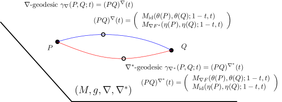
Figure 1: The points on dual geodesics in a dually flat spaces have dual coordinates expressed with quasi-arithmetic averages.

In a DFS $(M,g,\nabla,\nabla^{*})=\mathrm{DFS}(F,\theta\in\Theta;F^{*},\eta\in H)$, the primal geodesics $\gamma_{\nabla}(P,Q;t)$ are obtained as line segments in the $\theta$-coordinate system (because the Christoffel symbols of the connection $\nabla$ vanishes in the $\theta$-coordinate system) while the dual geodesics $\gamma_{\nabla^{*}}(P,Q;t)$ are line segments in the $\eta$-coordinate system (because the Christoffel symbols of the dual connection $\nabla^{*}$ vanishes in the $\eta$-coordinate system). The dual geodesics define interpolation schemes $(PQ)^{\nabla}(t)=\gamma_{\nabla}(P,Q;t)$ and $(PQ)^{\nabla^{*}}(t)=\gamma_{\nabla^{*}}(P,Q;t)$ between input points $P$ and $Q$ with $P=\gamma_{\nabla}(P,Q;0)=\gamma_{\nabla^{*}}(P,Q;0)$ and $Q=\gamma_{\nabla}(P,Q;1)=\gamma_{\nabla^{*}}(P,Q;1)$ when $t$ ranges in $[0,1]$. We express the coordinates of the interpolated points on $\gamma_{\nabla}$ and $\gamma_{\nabla^{*}}$ using quasi-arithmetic averages as follows (Figure 1):

$$(PQ)^{\nabla}(t) = \gamma_{\nabla}(P,Q;t)={\left[\begin{array}[]{ll}M_{\mathrm{id}}(\theta(P),\theta(Q);1-t,t)\cr M_{\nabla F^{*}}(\eta(P),\eta(Q);1-t,t)\end{array}\right]},$$ (8)

$$(PQ)^{\nabla^{*}}(t) = \gamma_{\nabla^{*}}(P,Q;t)={\left[\begin{array}[]{ll}M_{\nabla F}(\theta(P),\theta(Q);1-t,t)\cr M_{\mathrm{id}}(\eta(P),\eta(Q);1-t,t)\end{array}\right]}.$$ (11)

Quasi-arithmetic averages were used by a geodesic bisection algorithm to approximate the circumcenter of the minimum enclosing balls with respect to the canonical divergence in a DFS in [58].

3.2 Quasi-arithmetic average coordinates of dual barycenters with respect to the canonical divergence

Consider a finite set of $n$ points $P_{1},\ldots,P_{n}$ on the DFS $(M,g,\nabla,\nabla^{*})$. The points $P_{i}\,{\left[\begin{array}[]{ll}\theta_{i}\cr\eta_{i}\end{array}\right]}$ can be expressed in the dual coordinate systems either as $\theta(P_{i})=\theta_{i}$ or $\eta(P_{i})=\eta_{i}$. The right centroid point $\bar{C}_{R}\in M$ defined by $\bar{C}_{R}=\arg\min_{P\in M}\sum_{i=1}^{n}\frac{1}{n}D_{\nabla,\nabla^{*}}(P_{i}:P)$ (or equivalently as a right-sided Bregman centroid [13] $\bar{\theta}_{R}=\arg\min_{\theta}\sum_{i=1}^{n}\frac{1}{n}B_{F}(\theta_{i}:\theta)$) has dual coordinates

$$\bar{\theta}_{R} = \theta(\bar{C}_{R})=\frac{1}{n}\sum_{i=1}^{n}\theta_{i}=M_{\mathrm{id}}(\theta_{1},\ldots,\theta_{n}),$$ (12)

$$\bar{\eta}_{R} = \nabla F(\bar{\theta}_{R})=M_{\nabla F^{*}}(\eta_{1},\ldots,\eta_{n}).$$ (13)

Similarly, the left centroid point $\bar{C}_{L}\in M$ defined by $\bar{C}_{L}=\arg\min_{P\in M}\sum_{i=1}^{n}\frac{1}{n}D_{\nabla,\nabla^{*}}(P:P_{i})$ (or equivalently a left-sided Bregman centroid [54] $\bar{\theta}_{L}=\arg\min_{\theta}\sum_{i=1}^{n}\frac{1}{n}B_{F}(\theta:\theta_{i})$) has coordinates

$$\bar{\theta}_{L} = M_{\nabla F}(\theta_{1},\ldots,\theta_{n}),$$ (14)

$$\bar{\eta}_{L} = \nabla F(\bar{\theta}_{L})=M_{\mathrm{id}}(\eta_{1},\ldots,\eta_{n}).$$ (15)

Thus we have the two dual sided centroids $\bar{C}_{R}$ and $\bar{C}_{L}$ (reference duality [68]) on the dually flat manifold $M$ expressed using the dual coordinates as

$$\bar{C}_{R}\,{\left[\begin{array}[]{ll}\bar{\theta}_{L}=M_{\nabla F}(\theta_{1},\ldots,\theta_{n})\cr\bar{\eta}_{L}=\nabla F(\bar{\theta}_{L})=M_{\mathrm{id}}(\eta_{1},\ldots,\eta_{n})\end{array}\right]},\quad\bar{C}_{L}\,{\left[\begin{array}[]{ll}\bar{\theta}_{L}=M_{\nabla F}(\theta_{1},\ldots,\theta_{n})\cr\bar{\eta}_{L}=\nabla F(\bar{\theta}_{L})=M_{\mathrm{id}}(\eta_{1},\ldots,\eta_{n})\end{array}\right]}$$

Let $\underline{\theta}=\frac{1}{n}\sum_{i=1}^{n}\theta_{i}$ and $\underline{\eta}=\frac{1}{n}\sum_{i=1}^{n}\eta_{i}$. Then we have $\underline{\theta}=\nabla F^{*}(M_{\nabla F^{*}}(\eta_{1},\ldots,\eta_{n}))$ and $\underline{\eta}=\nabla F(M_{\nabla F}(\theta_{1},\ldots,\theta_{n}))$ . The dual DFS centroids [60] were studied as Bregman sided centroids and expressed as quasi-arithmetic averages in [54].

Figure 2: Dual centroids in a dually flat spaces have dual coordinates expressed with quasi-arithmetic averages.

Figure 2 illustrates the dual centroids expressed using the quasi-arithmetic averages.

We may consider the barycenter of $n$ weighted points $P_{1},\ldots,P_{n}$ (weight vector $w\in\Delta_{n-1}$) with respect to a Jensen divergence [52] $J_{F}$ defined as the minimization of $\sum_{i=1}^{n}w_{i}J_{F}(\theta,\theta_{i})$. In [52], the following iterative algorithm was proposed: Let $\theta^{(0)}=\sum_{i=1}^{n}w_{i}\theta_{i}$, and iteratively update $\theta^{(t+1)}=M_{\nabla F}\left(\frac{\theta^{(t)}+\theta_{i}}{2},\ldots,\frac{\theta^{(t)}+\theta_{n}}{2};w\right)$.

3.3 Tripartite duality of densities/divergences/means and dual quasi-arithmetic averages

Banerjee et al. [13] proved a bijection between natural regular exponential families $\mathcal{E}_{F}=\{p_{\theta}(x)=\exp(x\cdot\theta-F(\theta))\}$ with cumulant functions $F$ and “regular” dual Bregman divergences $B_{F^{*}}$ by rewriting the densities as $p_{\theta}(x)=p_{\eta}(x)=\exp(-B_{F^{*}}(x:\eta)+F^{*}(x))$ with $\eta=\nabla F(\theta)$ (using the Young equality $F(\theta)+F^{*}(\eta)-\left\langle\theta,\eta\right\rangle=0$). Furthermore, a bijection between Bregman divergences $B_{F}$ and quasi-arithmetic averages $M_{\nabla F}$ was informally mentioned in [58]. Using these bijections, we can cast the maximum likelihood estimator (MLE) of an exponential family $\mathcal{E}_{F}$ as a dual right-sided Bregman centroid problem [46]. Figure 3 summarizes the dualities between convex conjugate functions, exponential families and Bregman divergences, and maximum likelihood estimator, Bregman centroid expressed as multivariate QAMs.

The categorical mean of Example 2 is induced by the gradient map of the cumulant function of the exponential family of categorical distributions [7] (the family of discrete distributions on a finite alphabet).

Figure 3: Overview of the bijections between regular exponential families, Bregman divergences of Legendre-type, and quasi-arithmetic averages.

A Legendre-type function $F$ induces two dual quasi-arithmetic weighted averages $M_{\nabla F}$ and $M_{\nabla F^{*}}$ by the gradient maps of the convex conjugates $F$ and $F^{*}$.

When $\nabla F=\nabla F^{*}=\nabla F^{-1}$ (meaning that the convex conjugate gradients are reciprocal to each others), we have $M_{\nabla F}=M_{\nabla F^{*}}$. This holds for example for the scalar and matrix harmonic means which are self-dual means with $\nabla F(x)=x^{-1}=\nabla F^{*}(x)$.

Consider the Mahalanobis divergence $\Delta^{2}$ (i.e., the squared Mahalanobis distance $\Delta$) as a Bregman divergence obtained for the quadratic form generator $F_{Q}(\theta)=\frac{1}{2}\theta^{\top}Q\theta+c\theta+\kappa$ for a symmetric positive-definite $d\times d$ matrix $Q$, $c\in\mathbb{R}^{d}$ and $\kappa\in\mathbb{R}$. We have:

$$\Delta^{2}(\theta_{1},\theta_{2})=B_{F_{Q}}(\theta_{1}:\theta_{2})=\frac{1}{2}(\theta_{2}-\theta_{1})^{\top}Q(\theta_{2}-\theta_{1}).$$

When $Q=I$, the identity matrix, the Mahalanobis divergence coincides with the Euclidean divergence (i.e., the squared Euclidean distance). The Legendre convex conjugate is $F^{*}(\eta)=\frac{1}{2}\eta^{\top}Q^{-1}\eta=F_{Q^{-1}}(\eta)$, and we have $\eta=\nabla F_{Q}(\theta)=Q\theta$ and $\theta=\nabla F^{*}_{Q}(\eta)=Q^{-1}\eta$. Thus we get the following dual quasi-arithmetic averages:

$$M_{\nabla F_{Q}}(\theta_{1},\ldots,\theta_{n};w) = Q^{-1}\left(\sum_{i=1}^{n}w_{i}Q\theta_{i}\right)=\sum_{i=1}^{n}w_{i}\theta_{i}=M_{\mathrm{id}}(\theta_{1},\ldots,\theta_{n};w),$$ (16)

$$M_{\nabla F_{Q}^{*}}(\eta_{1},\ldots,\eta_{n};w) = Q\left(\sum_{i=1}^{n}w_{i}Q^{-1}\eta_{i}\right)=M_{\mathrm{id}}(\eta_{1},\ldots,\eta_{n};w).$$ (17)

The dual quasi-arithmetic average functions $M_{\nabla F_{Q}}$ and $M_{\nabla F_{Q}^{*}}$ induced by a Mahalanobis Bregman generator $F_{Q}$ coincide since $M_{\nabla F_{Q}}=M_{\nabla F_{Q}^{*}}=M_{\mathrm{id}}$. This means geometrically that the left-sided and right-sided centroids of the underlying canonical divergences match. The average $M_{\nabla F_{Q}}(\theta_{1},\ldots,\theta_{n};w)$ expresses the centroid $C=\bar{C}_{R}=\bar{C}_{L}$ in the $\theta$-coordinate system ($\theta(C)=\underline{\theta}$) and the average $M_{\nabla F_{Q}^{*}}(\eta_{1},\ldots,\eta_{n};w)$ expresses the same centroid in the $\eta$-coordinate system ($\eta(C)=\underline{\eta}$). In that case of self-dual flat Euclidean geometry, there is an affine transformation relating the $\theta$- and $\eta$-coordinate systems:$\eta=Q\theta$ and $\theta=Q^{-1}\eta$. As we shall see this is because the underlying geometry is self-dual Euclidean flat space $(M,g_{\mathrm{Euclidean}},\nabla_{\mathrm{Euclidean}},\nabla_{\mathrm{Euclidean}}^{*}=\nabla_{\mathrm{Euclidean}})$ and that both dual connections coincide with the Euclidean connection (i.e., the Levi-Civita connection of the Euclidean metric). In this particular case, the dual coordinate systems are just related by affine transformations of one to another.

3.4 Quasi-arithmetic averages and the inductive matrix geometric mean

Consider $P$ and $Q$ two symmetric positive-definite (SPD) matrices of $\mathrm{Sym}_{++}(d)$. By equipping the SPD cone $\mathrm{Sym}_{++}(d)$ with the Riemannian trace metric

$$g_{P}(X,Y)=\mathrm{tr}\left(P^{-1}X\,P^{-1}Y\right)$$

where $X$ and $Y$ are symmetric matrices of the tangent plane $T_{p}$ identified with the vector space $\mathrm{Sym}(d)$, we get a Riemannian manifold $(\mathrm{Sym}_{++}(d),g)$ with geodesic distance [31]:

$$\rho(P,Q)=\sqrt{\sum_{i=1}^{d}\log^{2}\lambda_{i}(P^{-\frac{1}{2}}\,Q\,P^{-\frac{1}{2}})},$$

where $\lambda_{i}$ denote the $i$-th largest real-valued eigenvalue of the SPD matrix $P^{-\frac{1}{2}}\,Q\,P^{-\frac{1}{2}}$. The Riemannian center of mass $P^{*}$ of $n$ points $P_{1}$, …, $P_{n}$ (commonly called centroid or Kärcher mean) is defined as

$$P^{*}=\arg\min_{P\in\mathrm{Sym}_{++}(d)}\frac{1}{n}\sum_{i=1}^{n}\rho^{2}(P_{i},P).$$

Since the SPD Riemannian manifold $(\mathrm{Sym}_{++}(d),g)$ is of non-positive sectional curvatures ranging in $[-\frac{1}{2},0]$, the Riemannian centroid $P^{*}$ is unique. In particular, when $n=2$, we get

$$P^{*}=P_{1}^{\frac{1}{2}}\,\left(P_{1}^{-\frac{1}{2}}\,P_{2}\,P_{1}^{-\frac{1}{2}}\right)^{\frac{1}{2}}\,P_{1}^{\frac{1}{2}}$$

which coincides with one usual definition [8, 16] of the geometric matrix mean $G(P_{1},P_{2})$ where

$$G(P,Q)=Q^{\frac{1}{2}}\left(Q^{-\frac{1}{2}}\,P\,Q^{-\frac{1}{2}}\right)^{\frac{1}{2}}Q^{\frac{1}{2}},$$

Nakamura [43] considered the following iterations based on the arithmetic matrix mean $A(P,Q)=(P+Q)/2$ and harmonic matrix mean $H(P,Q)=2\,((P^{-1}+Q^{-1}))^{-1}$:

$$P_{t+1} = \frac{P_{t}+Q_{t}}{2}=:A(P_{t},Q_{t}),$$ (18)

$$Q_{t+1} = 2\,(P_{t}^{-1}+Q_{t}^{-1})^{-1}=:H(P_{t},Q_{t}),$$ (19)

initialized with $P_{0}=P$ and $Q_{0}=Q$. Let $M(P,Q)=\lim_{t\rightarrow\infty}P_{t}$. It is proven that $M(P,Q)=\lim_{t\rightarrow\infty}Q_{t}$, and

$$M(P,I)=P^{\frac{1}{2}},$$

the square-root matrix, and

$$M(P,Q)=G(P,Q).$$

Furthermore, the convergence is quadratic [43, 10].

We can extend $(\mathrm{Sym}_{+}+(d),g)$ as a dually flat space $(\mathrm{Sym}_{+}+(d),g,\nabla,\nabla^{*})$ where $\nabla$ is the flat Levi-Civita connection induced by the Euclidean metric $\stackrel{{\scriptstyle E}}{{g}}_{P}(X,Y)=\mathrm{tr}(XY)$ and $\nabla^{*}$ is the flat Levi-Civita connection induced by the so-called inverse Euclidean metric [64, 65] $\stackrel{{\scriptstyle\mathrm{IE}}}{{g}}_{P}(X,Y)=\mathrm{tr}\left(P^{-2}XP^{-2}Y\right)$ (isometric to the Euclidean metric). The non-flat trace metric $g$ is interpreted as a balanced bilinear form [64]. The midpoint $\nabla$-geodesic corresponds to the arithmetic mean and the midpoint $\nabla^{*}$-geodesic corresponds to the matrix harmonic mean. The iterations of Eq. 18 and Eq. 19 converging to the Riemannian center of mass can thus be interpreted geometrically on the dually flat space $(\mathrm{Sym}_{+}+(d),g,\nabla,\nabla^{*})$ (see Figure 4), with the geodesic midpoints expressed as quasi-arithmetic averages $M_{X}$ and $M_{X^{-}1}$ which are the gradient maps of Legendre-type functions $\frac{1}{2}\mathrm{tr}(X^{2})$ and $-\log\mathrm{det}(X)$, respectively.

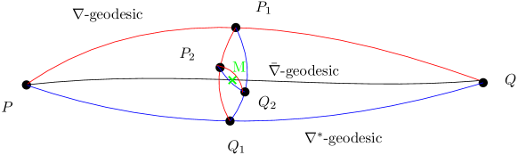
Figure 4: The points on dual geodesics in a dually flat spaces have dual coordinates expressed with quasi-arithmetic averages.

The inductive process is further generalized to Hilbert spaces of functions with the arithmetic and harmonic matrix means being replaced by the arithmetic average function $A(p,q)=\frac{p+q}{2}$ and a harmonic-type function $hH(p,q)=\left(\frac{p^{*}+q^{*}}{2}\right)^{*}$ defined using the Legendre transform in [10].

4 Invariance and equivariance properties of quasi-arithmetic averages

Recall that a dually flat manifold [7] $(M,g,\nabla,\nabla^{*})$ has a canonical divergence [5] $D_{\nabla,\nabla^{*}}$ which can be expressed either as a primal Bregman divergence in the $\nabla$-affine coordinate system $\theta$ (using the convex potential function $F(\theta)$) or as a dual Bregman divergence in the $\nabla^{*}$-affine coordinate system $\eta$ (using the convex conjugate potential function $F^{*}(\eta)$), or as dual Fenchel-Young divergences [50] using the mixed coordinate systems $\theta$ and $\eta$. The dually flat manifold $(M,g,\nabla,\nabla^{*})$ (a particular case of Hessian manifolds [62] which admit a global coordinate system) is characterized by $(\theta,F(\theta);\eta,F^{*}(\eta))$ which we shall denote by $(M,g,\nabla,\nabla^{*})\leftarrow\mathrm{DFS}(\theta,F(\theta);\eta,F^{*}(\eta))$ (or in short $(M,g,\nabla,\nabla^{*})\leftarrow(\Theta,F(\theta))$). However, the choices of parameters $\theta$ and $\eta$ and potential functions $F$ and $F^{*}$ are not unique since they can be chosen up to affine reparameterizations and additive affine terms [7]: $(M,g,\nabla,\nabla^{*})\leftarrow\mathrm{DFS}([\theta,F(\theta);\eta,F^{*}(\eta)])$ where $[\cdot]$ denotes the equivalence class that has been called purposely the affine Legendre invariance in [42]:

• First, consider changing the potential function $F(\theta)$ by adding an affine term: ${\bar{F}}(\theta)=F(\theta)+\left\langle c,\theta\right\rangle+d$. We have $\nabla{\bar{F}}(\theta)=\nabla F(\theta)+c=\bar{\eta}$. Inverting $\nabla{\bar{F}}(x)=\nabla F(x)+c=y$, we get $\nabla{\bar{F}}^{-1}(y)=\nabla F(y-c)$. We check that $B_{F}(\theta_{1}:\theta_{2})=B_{\bar{F}}(\theta_{1}:\theta_{2})=D_{\nabla,\nabla^{*}}(P_{1}:P_{2})$ with $\theta(P_{1})=:\theta_{1}$ and $\theta(P_{2})=:\theta_{2}$. It is indeed well-known that Bregman divergences modulo affine terms coincide [13]. For the quasi-arithmetic averages $M_{\nabla{\bar{F}}}$ and $M_{\nabla F}$, we thus obtain the following invariance property: $M_{\nabla{\bar{F}}}(\theta_{1},\ldots;\theta_{n};w)=M_{\nabla F}(\theta_{1},\ldots;\theta_{n};w)$.

• Second, consider an affine change of coordinates ${\bar{\theta}}=A\theta+b$ for $A\in\mathrm{GL}(d)$ and $b\in\mathbb{R}^{d}$, and define the potential function ${\bar{F}}({\bar{\theta}})$ such that ${\bar{F}}({\bar{\theta}})=F(\theta)$. We have $\theta=A^{-1}({\bar{\theta}}-b)$ and ${\bar{F}}(x)=F(A^{-1}(x-b))$. It follows that $\nabla{\bar{F}}(x)=(A^{-1})^{\top}\nabla F(A^{-1}(x-b))$, and we check that $B_{{\bar{F}}(\overline{\theta_{1}}:\overline{\theta_{2}})}=B_{F}(\theta_{1}:\theta_{2})$:

  $$B_{{\bar{F}}(\overline{\theta_{1}}:\overline{\theta_{2}})} = {\bar{F}}(\overline{\theta_{1}})+{\bar{F}}(\overline{\theta_{2}})-\left\langle\overline{\theta_{1}}-\overline{\theta_{2}},\nabla{\bar{F}}(\overline{\theta_{2}})\right\rangle,$$

  $$= F(\theta_{1})-F(\theta_{2})-(A(\theta_{1}-\theta_{2}))^{\top}(A^{-1})^{\top}\nabla F(\theta_{2}),$$

  $$= F(\theta_{1})-F(\theta_{2})-(\theta_{1}-\theta_{2})^{\top}\underbrace{A^{\top}(A^{-1})^{\top}}_{(A^{-1}A)^{\top}=I}\nabla F(\theta_{2})=B_{F}(\theta_{1}:\theta_{2}).$$

  This highlights the invariance that $D_{\nabla,\nabla^{*}}(P_{1}:P_{2})=B_{F}(\theta_{1}:\theta_{2})=B_{{\bar{F}}({\bar{\theta}}_{1}:{\bar{\theta}}_{2})}$, i.e., the canonical divergence does not change under a reparameterization of the $\nabla$-affine coordinate system. For the induced quasi-arithmetic averages $M_{\nabla{\bar{F}}}$ and $M_{\nabla F}$, we have $\nabla{\bar{F}}(x)=(A^{-1})^{\top}\nabla F(A^{-1}(x-b))=y$, we calculate $x=\nabla{\bar{F}}(x)^{1}(y)=A\,\nabla{\bar{F}}^{-1}(((A^{-1})^{\top})^{-1}y)+b$, and we have

  $$M_{\nabla{\bar{F}}}(\overline{\theta_{1}},\ldots,\overline{\theta_{n}};w) := \nabla{\bar{F}}^{-1}(\sum_{i}w_{i}\nabla{\bar{F}}(\overline{\theta_{i}})),$$

  $$= (\nabla{\bar{F}})^{-1}\left((A^{-1})^{\top}\sum_{i}w_{i}\nabla F(\theta_{i})\right),$$

  $$= A\,\nabla F^{-1}\left(\underbrace{((A^{-1})^{\top})^{-1}(A^{-1})^{\top}}_{=I}\sum_{i}w_{i}\nabla F(\theta_{i})\right),$$

  $$M_{\nabla{\bar{F}}}(\overline{\theta_{1}},\ldots,\overline{\theta_{n}};w) = A\,M_{\nabla F}(\theta_{1},\ldots,\theta_{n};w)+b$$

  More generally, we may define $\bar{F}({\bar{\theta}})=F(A\theta+b)+\left\langle c,\theta\right\rangle+d$ and get via Legendre transformation $\bar{F}^{*}({\bar{\eta}})=F^{*}(A^{*}\eta+b^{*})+\left\langle c^{*},\eta\right\rangle+d^{*}$ (with $A^{*},b^{*},c^{*}$ and $d^{*}$ expressed using $A,b,c$ and $d$ since these parameters are linked by the Legendre transformation).

• Third, the canonical divergences should be considered relative divergences (and not absolute divergences), and defined according to a prescribed arbitrary “unit” $\lambda>0$. Thus we can scale the canonical divergence by $\lambda>0$, i.e., $D_{\lambda,\nabla,\nabla^{*}}:=\lambda D_{\nabla,\nabla^{*}}$. We have $D_{\lambda,\nabla,\nabla^{*}}(P_{1}:P_{2})=\lambda B_{F}(\theta_{1}:\theta_{2})=\lambda B_{F^{*}}(\eta_{2}:\eta_{1})=\lambda Y_{F}(\theta_{1}:\eta_{2})=\lambda Y_{F^{*}}(\eta_{1}:\theta_{2})$, and $\lambda B_{F}(\theta_{1}:\theta_{2})=B_{\lambda F}(\theta_{1}:\theta_{2})$ (and $\nabla\lambda F=\lambda\nabla F$). We check the scale invariance of quasi-arithmetic averages: $M_{\lambda\nabla F}=M_{\nabla F}$.

Thus we end up with the following invariance and equivariance properties of the quasi-arithmetic averages which have been obtained from an information-geometric viewpoint:

Proposition 2 (Invariance and equivariance of quasi-arithmetic averages)

Let $F(\theta)$ be a function of Legendre type. Then $\bar{F}({\bar{\theta}}):=\lambda(F(A\theta+b)+\left\langle c,\theta\right\rangle+d)$ for $A\in\mathrm{GL}(d)$, $b,c\in\mathbb{R}^{d}$, $d\in\mathbb{R}^{d}$ and $\lambda\in\mathbb{R}_{>0}$ is a Legendre-type function, and we have $M_{\nabla\bar{F}}=A\,M_{\nabla F}+b$.

This proposition generalizes Property 1 of scalar QAMs, and untangles the role of scale $\lambda>0$ from the other invariance roles brought by the Legendre transformation.

5 Quasi-arithmetic statistical mixtures and information geometry

5.1 Definition of quasi-arithmetic statistical mixtures

Consider a quasi-arithmetic mean $m_{f}$. We consider $n$ probability distributions $P_{1},\ldots,P_{n}$ all dominated by a measure $\mu$, and denote by $p_{1}=\frac{\mathrm{d}P_{1}}{\mathrm{d}\mu},\ldots,p_{n}=\frac{\mathrm{d}P_{n}}{\mathrm{d}\mu}$ their Radon-Nikodym derivatives. Let us define statistical $m_{f}$-mixtures of $p_{1},\ldots,p_{n}$:

Definition 4

The $m_{f}$-mixture of $n$ densities $p_{1},\ldots,p_{n}$ weighted by $w\in\Delta_{n}^{\circ}$ is defined by

$$(p_{1},\ldots,p_{n};w)^{m_{f}}(x):=\frac{m_{f}(p_{1}(x),\ldots,p_{n}(x);w)}{\int m_{f}(p_{1}(x),\ldots,p_{n}(x);w)\mathrm{d}\mu(x)}.$$

The quasi-arithmetic mixture (QAMIX for short) $(p_{1},\ldots,p_{n};w)^{m_{f}}$ generalizes the ordinary statistical mixture $\sum_{i=1}^{d}w_{i}p_{i}(x)$ when $f(t)=t$ and $m_{f}=A$ is the arithmetic mean. A statistical $m_{f}$-mixture can be interpreted as the $m_{f}$-integration of its weighted component densities, the densities $p_{i}$’s. The power mixtures $(p_{1},\ldots,p_{n};w)^{m_{p}}(x)$ (including the ordinary and geometric mixtures) are called $\alpha$-mixtures in [6] with $\alpha(p)=1-2p$ (or $p=\frac{1-\alpha}{2}$). A nice characterization of the $\alpha$-mixtures is that these mixtures are the density centroids of the weighted mixture components with respect to the $\alpha$-divergences [6] (proven by calculus of variation):

$$(p_{1},\ldots,p_{n};w)^{m_{\alpha}}=\arg\min_{p}w_{i}D_{\alpha}(p_{i},p),$$

where $D_{\alpha}$ denotes the $\alpha-$divergences [7, 57]. $m_{f}$-mixtures have also been used to define a generalization of the Jensen-Shannon divergence [48] between densities $p$ and $q$ as follows:

$$D_{\mathrm{JS}}^{m_{f}}(p,q):=\frac{1}{2}\left(D_{\mathrm{KL}}(p:(pq)^{m_{f}})+D_{\mathrm{KL}}(q:(pq)^{m_{f}})\right)\geq 0,$$ (20)

where $D_{\mathrm{KL}}(p:q)=\int p(x)\log\frac{p(x)}{q(x)}\mathrm{d}\mu(x)$ is the Kullback-Leibler divergence, and $(pq)^{m_{f}}:=(p,q;\frac{1}{2},\frac{1}{2})^{m_{f}}$. The ordinary JSD is recovered when $f(t)=t$ and $m_{f}=A$:

$$D_{\mathrm{JS}}(p,q)=\frac{1}{2}\left(D_{\mathrm{KL}}\left(p:\frac{p+q}{2}\right)+D_{\mathrm{KL}}\left(q:\frac{p+q}{2}\right)\right).$$

Quasi-arithmetic mixtures of two components have also been used to upper bound the probability of error in Bayesian hypothesis testing [47].

Let us give some examples of parametric families of probability distributions that are closed under quasi-arithmetic mixturing:

• Consider a natural exponential family [14] $\mathcal{E}=\{p_{\theta}=\exp(\theta\cdot x-F(\theta))\ :\ \theta\in\Theta\}$. Function $F(\theta)=\log\int\exp(\theta\cdot x)\mathrm{d}\mu$ is called the cumulant function (the log-normalizer function called log-partition in statistical physics), and is of Legendre type when the exponential family is steep [14]. Regular exponential families with are full exponential families with open natural parameter spaces $\Theta$ are steep. We have Shannon entropy of density $p_{\theta}\in\mathcal{E}$ expressed using the negative convex conjugate [55] which is concave: $H(p_{\theta})=-F^{*}(\eta)$ with $\eta=\nabla F(\theta)$. Since exponential families are closed under geometric mixtures, i.e. $(p_{\theta_{1}}p_{\theta_{2}})^{G}=p_{\frac{\theta_{1}+\theta_{2}}{2}}$, we have Shannon entropy which can be expressed using the convex conjugate:

  $$H((p_{\theta_{1}}p_{\theta_{2}})^{G})=-F^{*}\left(\nabla F\left(\frac{\theta_{1}+\theta_{2}}{2}\right)\right).$$

  We can rewrite $\nabla F\left(\frac{\theta_{1}+\theta_{2}}{2}\right)$ as the quasi-arithmetic average $M_{\nabla F^{*}}(\eta_{1},\eta_{2})$. More generally, the geometric mixtures of $n$ densities of an exponential family belongs to that exponential family:

  $$(p_{\theta_{1}},\ldots,p_{\theta_{n}};w)^{G}\propto\prod_{i=1}^{n}p_{\theta_{i}}^{w_{i}}=p_{\sum_{i=1}^{n}w_{i}\theta_{i}}.$$

  That is the normalization constant of $\prod_{i=1}^{n}p_{\theta_{i}}^{w_{i}}$ is $\exp(F(\sum_{i}w_{i}F(\theta_{i}))-\sum w_{i}F(\theta_{i})=\exp(-J_{F}(\theta_{1},\ldots,\theta_{n};w))$, where $J_{F}$ is called the Jensen diversity index [22, 52].

  We may also build an exponential family by considering $n+1$ probability distributions $P_{0},\ldots,P_{n}$ mutually absolutely continuous and all dominated by a reference measure $\mu$. Let $p_{0},\ldots,p_{n}$ denote their Radon-Nikodym densities such that $\log\frac{p_{1}}{p_{0}},\ldots,\log\frac{p_{n}}{p_{0}}$ are linear independent. Then consider the geometric mixture family:

  $$\mathcal{G}=\left\{(p_{0},\ldots,p_{n};w)^{G}=\ :\ w\in\Delta_{n}^{\circ}\right\}.$$

  We have $(p_{0},p_{1},\ldots,p_{n};w)^{G}\propto\exp\left(\sum_{i=1}^{n}w_{i}\log\frac{p_{i}}{p_{0}}\right)p_{0}(x)$. We let the natural parameter be $\theta=(w_{1},\ldots,w_{n})\in\Delta_{n}^{\circ}$. When $n=1$, Grünwald [29] called $\mathcal{G}$ a likelihood ratio exponential family (LREF). Uni-order LREFs ($n=1$) have been studied in [20, 49]: It has the advantage of considering a non-parametric statistical model [68] as a 1D exponential family model which yields a convenient framework for studying the statistical model $\mathcal{G}$ under the lens of well-studied exponential families [14].

  Remark 2

  We may consider another equivalent definition of the ordinary JSD [63, 37] given by

  $$D_{\mathrm{JS}}(p,q)=H\left(\frac{p+q}{2}\right)-\frac{H(p)+H(q)}{2}\geq 0,$$ (21)

  where $H(p)=-\int p(x)\log p(x)\mathrm{d}\mu(x)$ is the strictly concave Shannon entropy. Thus we may consider the following generalization of the JSD:

  $$H_{\mathrm{JS}}^{M_{f},M_{g}}(p,q)=H\left((pq)^{m_{f}}\right)-m_{g}(H(p),H(q)),$$ (22)

  where $m_{f}$ and $m_{g}$ are two quasi-arithmetic means. The first QAM is used to build a quasi-arithmetic mixture while the second QAM is used to average scalars. When $f(t)=g(t)=t$, we recover the ordinary JSD with $m_{f}=m_{g}=A$. Let us introduce the $(M,N)$-Jensen divergences [56] according to two generic symmetric bivariate means $M$ and $N$:

  $$J_{F}^{M,N}(\theta_{1},\theta_{2})=M(F(\theta_{1}),F(\theta_{2}))-F(N(\theta_{1},\theta_{2})).$$ (23)

  We recover the ordinary Jensen divergence [22, 52] when $M=N=A$:

  $$J_{F}(\theta_{1},\theta_{2})=J_{F}^{A,A}(\theta_{1},\theta_{2})=\frac{F(\theta_{1})+F(\theta_{2})}{2}-F\left(\frac{\theta_{1}+\theta_{2})}{2}\right).$$

  Jensen divergences are non-negative and equal to zero only when $\theta_{1}=\theta_{2}$ when $F$ is a strictly convex function. Similarly, by definition, $J_{F}^{M,N}(\theta_{1},\theta_{2})\geq 0$ with equality only when $\theta_{1}=\theta_{2}$ when $F$ is said $(M,N)$-convex [45] and [44] (Appendix A). A $(G,A)$-convex function is said log-convex and a $(G,G)$-convex function is said multiplicative convex. We can test whether a function $g$ is strictly $(m_{f_{1}},m_{f_{2}})$-convex by checking whether the function $f_{2}\circ g\circ f_{1}$ is strictly convex or not (see the correspondence Lemma A.2.2 in [44]). For densities $p_{\theta_{1}}$ and $p_{\theta_{2}}$ belonging to a same exponential family $\mathcal{E}$, we have

  $$H_{\mathrm{JS}}^{G,A}(p_{\theta_{1}},p_{\theta_{2}}) = H((p_{\theta_{1}}p_{\theta_{2}})^{G})-A(H(p_{\theta_{1}}),H(p_{\theta_{2}})),$$

  $$= -F^{*}\left(M_{\nabla F^{*}}(\eta_{1},\eta_{2})\right)+\frac{F^{*}(\eta_{1})+F^{*}(\eta_{2})}{2}=J^{\nabla F^{*},A}_{F^{*}}(\eta_{1},\eta_{2}),$$

  where $J^{\nabla F^{*},A}$ is the $(\nabla F^{*},A)$-Jensen divergence defined according to two means. Thus we have $H_{\mathrm{JS}}^{G,A}(p_{\theta_{1}},p_{\theta_{2}})\geq 0$ iff $F^{*}$ is $(\nabla F^{*},A)$-convex.

  To see how $H_{\mathrm{JS}}^{G,A}$ differs from $D_{\mathrm{JS}}^{G}$ defined in [48], let us introduce the cross-entropy between $p$ and $q$: $H^{\times}(p:q)=-\int p(x)\log q(x)\mathrm{d}\mu(x)$. Then $D_{\mathrm{KL}}(p:q)=H^{\times}(p:q)-H(p)$ with $H(p)=H^{\times}(p:p)$, and we have

  $$D_{\mathrm{JS}}^{G}(p:q) = \frac{1}{2}\left(D_{\mathrm{KL}}(p:(pq)^{G})+D_{\mathrm{KL}}(q:(pq)^{G})\right)\geq 0,$$ (24)

  $$= \frac{1}{2}\left(H^{\times}(p:(pq)^{G})-H(p)+H^{\times}(q:(pq)^{G})-H(q)\right)\geq 0,$$ (25)

  $$= H^{\times}((pq)^{A}:(pq)^{G})-\frac{H(p)+H(q)}{2}\geq 0.$$ (26)

  However, we have $H_{\mathrm{JS}}^{G,A}(p:q)=H^{\times}((pq)^{G}:(pq)^{G})-\frac{H(p)+H(q)}{2}$. Therefore, the dissimilarity $H_{\mathrm{JS}}^{G,A}(p:q)$ can be potentially negative when $H^{\times}((pq)^{G}:(pq)^{G})\leq H^{\times}((pq)^{A}:(pq)^{G})$.

• Let $p_{0},p_{1},\ldots,p_{n}$ denotes $n+1$ linearly independent densities, and consider their (arithmetic/standard) mixture family [7]: $\mathcal{M}=\{m_{\theta}(x)=\sum_{i=0}^{n}w_{i}p_{i}(x)\ :\ w\in\Delta_{n}^{\circ}\}$ with $\theta=(w_{1},\ldots,w_{n})\in\Delta_{n-1}^{\circ}$ (and $w_{0}=1-\sum_{i=1}^{1}\theta_{i}$). The Shannon negentropy $F(\theta)=-H(m_{\theta})$ is a Legendre type function [53]. Since the mixture of two densities of a mixture family $\mathcal{M}$ belongs to $\mathcal{M}$ (i.e., $\frac{m_{\theta_{1}}+m_{\theta_{2}}}{2}=m_{\frac{\theta_{1}+\theta_{2}}{2}}$), we have $H\left(\frac{m_{\theta_{1}}+m_{\theta_{2}}}{2}\right)=H\left(m_{\frac{\theta_{1}+\theta_{2}}{2}}\right)=-F\left({\frac{\theta_{1}+\theta_{2}}{2}}\right)$. It follows that $D_{\mathrm{JS}}(m_{\theta_{1}}:m_{\theta_{2}})=J_{F}(\theta_{1}:\theta_{2})\geq 0$.

• Consider the family of scale Cauchy distributions $\mathcal{C}=\left\{p_{s}(x)=\frac{1}{\pi s}\frac{1}{1+\left(\frac{x}{s}\right)^{2}}\ :\ s\in\mathbb{R}_{>0}\right\}$. The harmonic mixture $(p_{s_{1}}p_{s_{2}})^{H}$ of two Cauchy distributions is a Cauchy distribution $p_{s_{12}}$ [47] with parameter $s_{12}=\sqrt{\frac{s_{1}s_{2}^{2}+s_{2}s_{1}^{2}}{s_{1}+s_{2}}}$. More generally, the harmonic mixtures of $n$ scale Cauchy distributions is a Cauchy distribution.

• The power mixture of central multivariate $t$-distributions is a central multivariate $t$-distribution [47] .

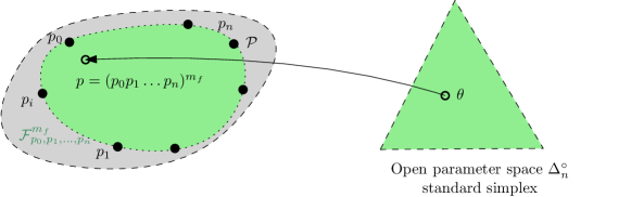
Figure 5: Statistical models in the quasi-mixture family are parametrized by a vector in the open standard simplex.

In general, we may consider quasi-arithmetic paths between densities on the space $\mathcal{P}$ of probability density functions with a common support all dominated by a reference measure. On $\mathcal{P}$, we can build a parametric statistical model called a $m$-mixture family of order $n$ as follows:

$$\mathcal{F}_{p_{0},p_{1},\ldots,p_{n}}^{m_{f}}:=\left\{(p_{0},p_{1},\ldots,p_{n};(\theta,1))^{m_{f}}\ :\ \theta\in\Delta^{\circ}_{n}\right\}.$$

In particular, power $q$-paths have been investigated in [39] with applications in annealing importance sampling and other Monte Carlo methods. The information geometry of such a density space with quasi-arithmetic paths has been investigated in [27] by considering quasi-arithmetic means with respect to a monotone increasing and concave function. See also [66, 28].

5.2 The $\nabla$-Jensen-Shannon divergences

We conclude by giving a geometric definition of a generalization of the Jensen-Shannon divergence on $\mathcal{P}$ according to an arbitrary affine connection [7, 68] $\nabla$:

Definition 5 (Affine connection-based $\nabla$-Jensen-Shannon divergence)

Let $\nabla$ be an affine connection on the space of densities $\mathcal{P}$, and $\gamma_{\nabla}(p,q;t)$ the geodesic linking density $p=\gamma_{\nabla}(p,q;0)$ to density $q=\gamma_{\nabla}(p,q;1)$. Then the $\nabla$-Jensen-Shannon divergence is defined by:

$$D^{\mathrm{JS}}_{\nabla}(p,q):=\frac{1}{2}\left(D_{\mathrm{KL}}\left(p:\gamma_{\nabla}\left(p,q;\frac{1}{2}\right)\right)+D_{\mathrm{KL}}\left(q:\gamma_{\nabla}\left(p,q;\frac{1}{2}\right)\right)\right).$$ (27)

When $\nabla=\nabla^{m}$ is chosen as the mixture connection [7], we end up with the ordinary Jensen-Shannon divergence since $\gamma_{\nabla^{m}}(p,q;\frac{1}{2})=\frac{p+q}{2}$. When $\nabla=\nabla^{e}$, the exponential connection, we get the geometric Jensen-Shannon divergence [48] since $\gamma_{\nabla^{e}}(p,q;\frac{1}{2})=(pq)^{G}$ is a statistical geometric mixture. We may choose the $\alpha$-connections of information geometry to define $\nabla$-Jensen-Shannon divergences (see Figure 6).

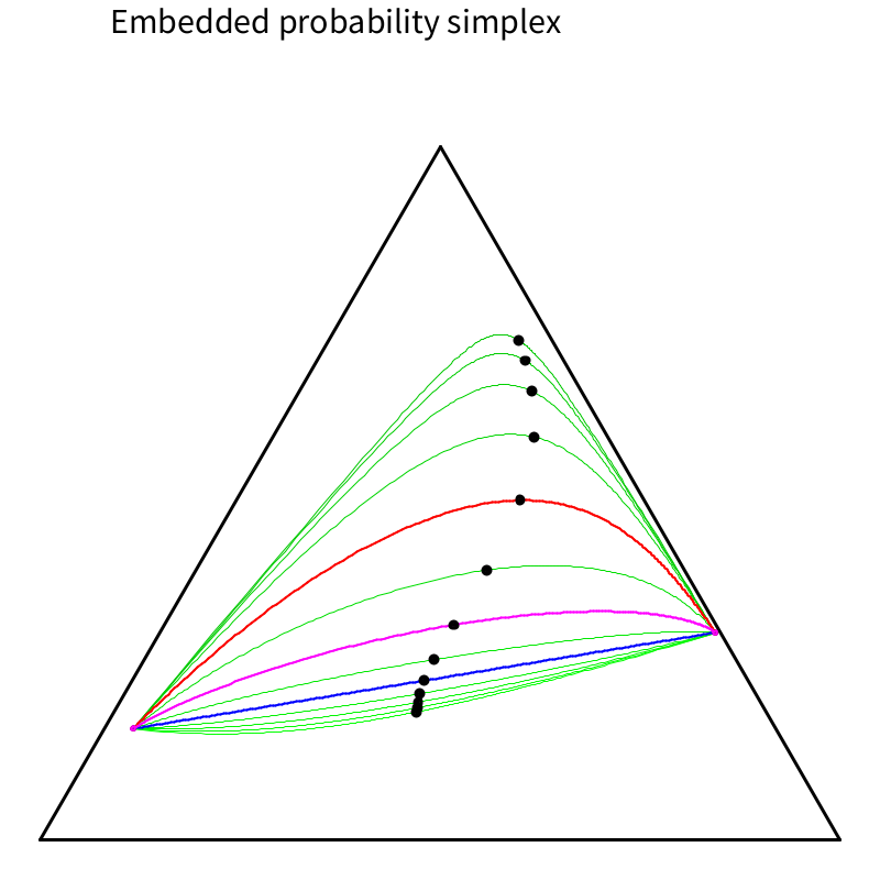
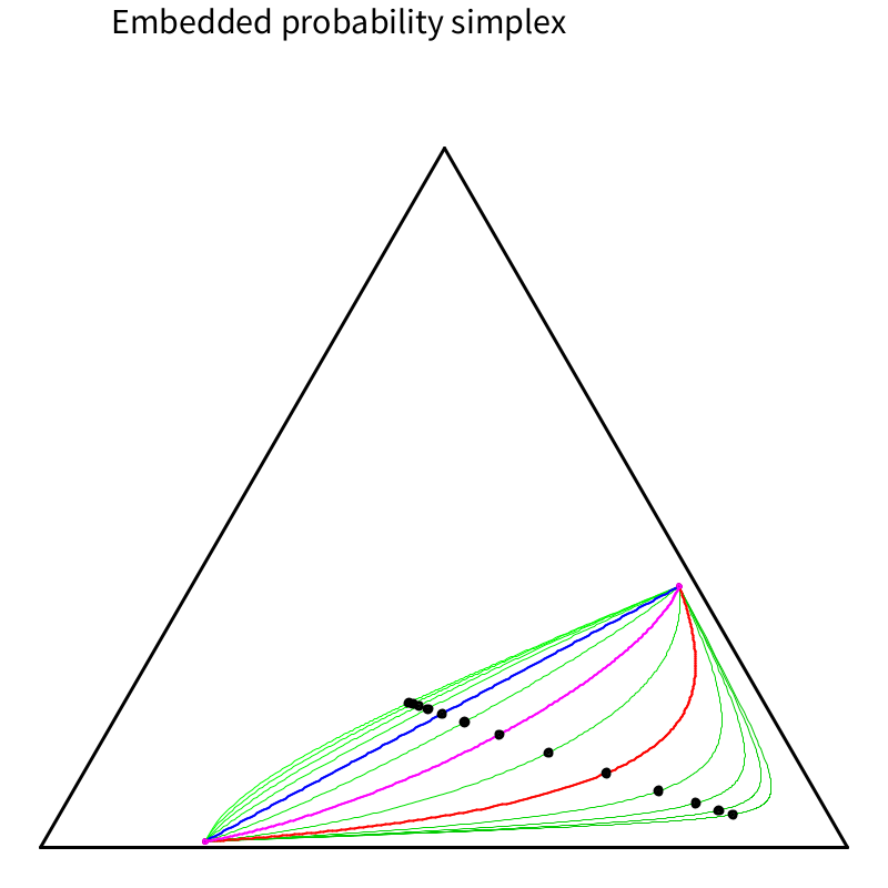
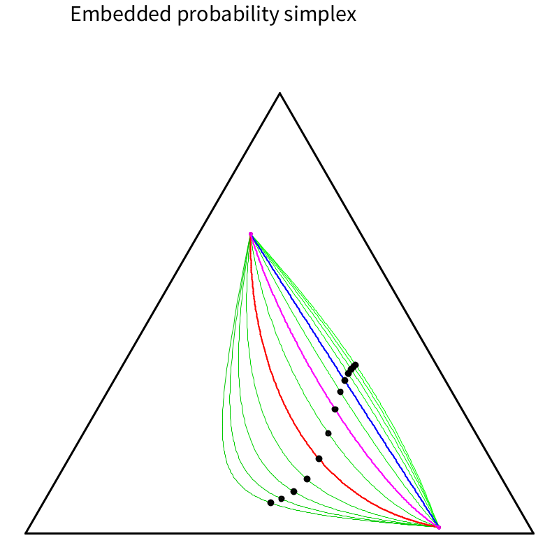
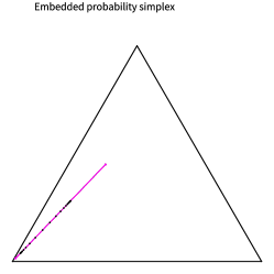
Figure 6: Top: Some $\alpha$-geodesics rendered in the 2D probability simplex (equilateral triangle sitting in 3D) with their midpoints displayed. Bottom: When the points $p$ and $q$ are collinear with a vertex of the probability simplex, the $\alpha$-geodesics coincide with the line $(pq)$.

When the space of densities $\mathcal{P}$ is a exponential family or a mixture family with carrying a dually flat structure $(\mathcal{P},g_{\mathrm{Fisher}},\nabla^{m},\nabla^{e})$ where $g_{\mathrm{Fisher}}$ denotes the Riemannian Fisher information metric [7], we have the Kullback-Leibler divergence $D_{\mathrm{KL}}$ which can be expressed using the canonical divergence $D_{\nabla^{m},\nabla^{e}}$, and the Jensen-Shannon divergence can be written geometrically as

$$D_{\mathrm{JS}}(p:q)=D^{\mathrm{JS}}_{\nabla}(P,Q):=\frac{1}{2}\left(D_{\nabla^{m},\nabla^{e}}\left(p:\gamma_{\nabla^{m}}(p,q;\frac{1}{2})\right)+D_{\nabla^{m},\nabla^{e}}\left(q:\gamma_{\nabla^{m}}(p,q;\frac{1}{2})\right)\right),$$

where $P$ and $Q$ denote the points on $\mathcal{P}$ representing the densities $p$ and $q$.

Furthermore, we may consider the $\alpha$-connections [7] $\nabla^{\alpha}$ of parametric or non-parametric statistical models, and skew the geometric Jensen-Shannon divergence to define the $\beta$-skewed $\nabla^{\alpha}$-JSD:

$$D^{\mathrm{JS}}_{\nabla^{\alpha},\beta}(p,q)=\beta D_{\mathrm{KL}}(p:\gamma_{\nabla^{\alpha}}(p,q;\beta))+(1-\beta)D_{\mathrm{KL}}(q:\gamma_{\nabla^{\alpha}}(p,q;\beta)).$$

6 Concluding remarks

In this paper, we presented two generalizations of the scalar quasi-arithmetic means [30] through the lens of information geometry, and discussed some of their applications:

• The first generalization of scalar quasi-arithmetic means consisted in defining pairs of quasi-arithmetic averages induced by the gradient maps of pairs of Legendre-type functions. These dual quasi-arithmetic averages are used in information geometry to express points on dual geodesics and sided barycenters in the dually affine $\theta$- and $\eta$-coordinate systems. Furthermore, we proved that $M_{\nabla F}=M_{\nabla\bar{F}}=M_{[\nabla F]}$ where $[\nabla\bar{F}]$ denotes the equivalence class of Legendre type functions such that $\bar{F}(\bar{\theta})=\lambda F(\theta+b)+\left\langle c,\theta\right\rangle+d\sim F(\theta)$. This property generalizes the well-known fact that quasi-arithmetic means $M_{f}=M_{g}$ iff $g=\lambda f+c$ and distinguishes the scaling invariance by $\lambda>0$ with the Legendre invariance by $c$.

• The second generalization of quasi-arithmetic means defined statistical quasi-arithmetic mixtures by normalizing quasi-arithmetic means of their densities: In particular, we showed how exponential families are closed under geometric mixtures, and described a generic way to build exponential families of order $n$ from geometric mixtures of $n+1$ linear independent log ratio densities $\log\frac{p_{i}}{p_{0}}$. The statistical geometric mixture family construction holds similarly for other quasi-arithmetic mixture families. Last, we gave a generic geometric definition of the Jensen-Shannon divergence based on affine connections which generalizes both the ordinary Jensen-Shannon divergence [37] and the geometric Jensen-Shannon divergence [48]. This demonstrates the rich interplay of divergences with information geometry.

References

- [1] S Abramovich, M Klaričić Bakula, M Matić, and J Pečarić. A variant of Jensen–Steffensen’s inequality and quasi-arithmetic means. Journal of mathematical analysis and applications, 307(1):370–386, 2005.
- [2] János Aczél. On mean values. Bull. Amer. Math. Soc., 54:392–400, 1948.
- [3] Yuichi Akaoka, Kazuki Okamura, and Yoshiki Otobe. Limit theorems for quasi-arithmetic means of random variables with applications to point estimations for the Cauchy distribution. Brazilian Journal of Probability and Statistics, 36(2):385–407, 2022.
- [4] M Alić, B Mond, J Pečarić, and V Volenec. The arithmetic-geometric-harmonic-mean and related matrix inequalities. Linear Algebra and its Applications, 264:55–62, 1997.
- [5] Shun-ichi Amari. Differential-geometrical methods in statistics. Lecture Notes on Statistics, 28:1, 1985.
- [6] Shun-ichi Amari. Integration of stochastic models by minimizing -divergence. Neural computation, 19(10):2780–2796, 2007.
- [7] Shun-ichi Amari. Information Geometry and Its Applications. Applied Mathematical Sciences. Springer Japan, 2016.
- [8] Tsuyoshi Ando, Chi-Kwong Li, and Roy Mathias. Geometric means. Linear algebra and its applications, 385:305–334, 2004.
- [9] Jesus Angulo. Morphological bilateral filtering. SIAM Journal on Imaging Sciences, 6(3):1790–1822, 2013.
- [10] Marc Atteia and Mustapha Raïssouli. Self dual operators on convex functionals; geometric mean and square root of convex functionals. Journal of Convex Analysis, 8(1):223–240, 2001.
- [11] Mahmut Bajraktarević. Sur une équation fonctionnelle aux valeurs moyennes. Glasnik Mat.-Fiz, 1958.
- [12] Miguel A Ballester and José Luis García-Lapresta. Using quasiarithmetic means in a sequential decision procedure. In EUSFLAT Conf.(2), pages 479–484, 2007.
- [13] Arindam Banerjee, Srujana Merugu, Inderjit S Dhillon, Joydeep Ghosh, and John Lafferty. Clustering with Bregman divergences. Journal of machine learning research, 6(10), 2005.
- [14] Ole Barndorff-Nielsen. Information and exponential families: in statistical theory. John Wiley & Sons, 2014.
- [15] Rajendra Bhatia, Stephane Gaubert, and Tanvi Jain. Matrix versions of the Hellinger distance. Letters in Mathematical Physics, 109(8):1777–1804, 2019.
- [16] Rajendra Bhatia and John Holbrook. Riemannian geometry and matrix geometric means. Linear algebra and its applications, 413(2-3):594–618, 2006.
- [17] Pierre-Alexandre Bliman, Alessio Carrozzo-Magli, Alberto d’Onofrio, and Piero Manfredi. Tiered social distancing policies and epidemic control. Proceedings of the Royal Society A, 478(2268):20220175, 2022.
- [18] Stephen Boyd, Stephen P Boyd, and Lieven Vandenberghe. Convex optimization. Cambridge university press, 2004.
- [19] Lev M. Bregman. The relaxation method of finding the common point of convex sets and its application to the solution of problems in convex programming. USSR computational mathematics and mathematical physics, 7(3):200–217, 1967.
- [20] Rob Brekelmans, Frank Nielsen, Alireza Makhzani, Aram Galstyan, and Greg Ver Steeg. Likelihood ratio exponential families. arXiv preprint arXiv:2012.15480, 2020.
- [21] Peter S Bullen, Dragoslav S Mitrinovic, and Means Vasic. Means and their inequalities, volume 31. Springer Science & Business Media, 2013.
- [22] Jacob Burbea and C Rao. On the convexity of some divergence measures based on entropy functions. IEEE Transactions on Information Theory, 28(3):489–495, 1982.
- [23] Tomasa Calvo, Gaspar Mayor, and Radko Mesiar. Aggregation operators: new trends and applications, volume 97. Springer Science & Business Media, 2002.
- [24] Francis Clarke. On the inverse function theorem. Pacific Journal of Mathematics, 64(1):97–102, 1976.
- [25] Marek Czachor and Jan Naudts. Thermostatistics based on Kolmogorov–Nagumo averages: unifying framework for extensive and nonextensive generalizations. Physics Letters A, 298(5-6):369–374, 2002.
- [26] Bruno De Finetti. Sul concetto di media. Istituto italiano degli attuari, 1931.
- [27] Shinto Eguchi and Osamu Komori. Path connectedness on a space of probability density functions. In Geometric Science of Information: Second International Conference, GSI 2015, Palaiseau, France, October 28-30, 2015, Proceedings 2, pages 615–624. Springer, 2015.
- [28] Shinto Eguchi, Osamu Komori, and Atsumi Ohara. Information geometry associated with generalized means. In Information Geometry and Its Applications: On the Occasion of Shun-ichi Amari’s 80th Birthday, IGAIA IV Liblice, Czech Republic, June 2016, pages 279–295. Springer, 2018.
- [29] Peter D Grünwald. The minimum description length principle. MIT press, 2007.
- [30] Godfrey Harold Hardy, John Edensor Littlewood, George Pólya, and György Pólya. Inequalities. Cambridge university press, 1952.
- [31] AT James. The variance information manifold and the functions on it. In Multivariate Analysis–III, pages 157–169. Elsevier, 1973.
- [32] Børge Jessen. Bemærkninger om konvekse Funktioner og Uligheder imellem Middelværdier. I. Matematisk tidsskrift. B, pages 17–28, 1931.
- [33] Konrad Knopp. Über reihen mit positiven gliedern. Journal of the London Mathematical Society, 1(3):205–211, 1928.
- [34] Andreĭ Nikolaevich Kolmogorov. Sur la notion de la moyenne. G. Bardi, tip. della R. Accad. dei Lincei, 12:388–391, 1930.
- [35] Osamu Komori and Shinto Eguchi. A unified formulation of -Means, fuzzy -Means and Gaussian mixture model by the Kolmogorov–Nagumo average. Entropy, 23(5):518, 2021.
- [36] Steven George Krantz and Harold R Parks. The implicit function theorem: History, theory, and applications. Springer Science & Business Media, 2002.
- [37] Jianhua Lin. Divergence measures based on the Shannon entropy. IEEE Transactions on Information theory, 37(1):145–151, 1991.
- [38] László Losonczi. Equality of two variable weighted means: reduction to differential equations. aequationes mathematicae, 58(3):223–241, 1999.
- [39] Vaden Masrani, Rob Brekelmans, Thang Bui, Frank Nielsen, Aram Galstyan, Greg Ver Steeg, and Frank Wood. -paths: Generalizing the geometric annealing path using power means. In Uncertainty in Artificial Intelligence, pages 1938–1947. PMLR, 2021.
- [40] Jadranka Micic, Zlatko Pavic, and Josip Pecaric Josip Pecaric. Jensen type inequalities on quasi-arithmetic operator means. Scientiae Mathematicae Japonicae, 73(2+ 3):183–192, 2011.
- [41] Mitio Nagumo. Über eine Klasse der Mittelwerte. In Japanese journal of mathematics: transactions and abstracts, volume 7, pages 71–79. The Mathematical Society of Japan, 1930.
- [42] Naomichi Nakajima and Toru Ohmoto. The dually flat structure for singular models. Information Geometry, 4(1):31–64, 2021.
- [43] Yoshimasa Nakamura. Algorithms associated with arithmetic, geometric and harmonic means and integrable systems. Journal of computational and applied mathematics, 131(1-2):161–174, 2001.
- [44] Constantin Niculescu and Lars-Erik Persson. Convex functions and their applications, volume 23. Springer, 2006.
- [45] Constantin P Niculescu. Convexity according to means. Mathematical Inequalities and Applications, 6:571–580, 2003.
- [46] Frank Nielsen. -MLE: A fast algorithm for learning statistical mixture models. In 2012 IEEE international conference on acoustics, speech and signal processing (ICASSP), pages 869–872. IEEE, 2012.
- [47] Frank Nielsen. Generalized Bhattacharyya and Chernoff upper bounds on Bayes error using quasi-arithmetic means. Pattern Recognition Letters, 42:25–34, 2014.
- [48] Frank Nielsen. On the Jensen–Shannon symmetrization of distances relying on abstract means. Entropy, 21(5):485, 2019.
- [49] Frank Nielsen. Revisiting Chernoff Information with Likelihood Ratio Exponential Families. Entropy, 24(10):1400, 2022.
- [50] Frank Nielsen. Statistical Divergences between Densities of Truncated Exponential Families with Nested Supports: Duo Bregman and Duo Jensen Divergences. Entropy, 24(3):421, 2022.
- [51] Frank Nielsen. Quasi-arithmetic centers, quasi-arithmetic mixtures, and the jensen-shannon -divergences. In Geometric Science of Information: 6th International Conference, GSI 2023, Saint-Malo, France, August 30-September 1st, 2023, Proceedings. Springer, 2023.
- [52] Frank Nielsen and Sylvain Boltz. The Burbea-Rao and Bhattacharyya centroids. IEEE Transactions on Information Theory, 57(8):5455–5466, 2011.
- [53] Frank Nielsen and Gaëtan Hadjeres. Monte Carlo information-geometric structures. In Geometric Structures of Information, pages 69–103. Springer, 2019.
- [54] Frank Nielsen and Richard Nock. Sided and symmetrized Bregman centroids. IEEE Transactions on Information Theory, 55(6):2882–2904, 2009.
- [55] Frank Nielsen and Richard Nock. Entropies and cross-entropies of exponential families. In 2010 IEEE International Conference on Image Processing, pages 3621–3624. IEEE, 2010.
- [56] Frank Nielsen and Richard Nock. Generalizing skew Jensen divergences and Bregman divergences with comparative convexity. IEEE Signal Processing Letters, 24(8):1123–1127, 2017.
- [57] Frank Nielsen, Richard Nock, and Shun-ichi Amari. On clustering histograms with -means by using mixed -divergences. Entropy, 16(6):3273–3301, 2014.
- [58] Richard Nock and Frank Nielsen. Fitting the smallest enclosing Bregman ball. In European Conference on Machine Learning, pages 649–656. Springer, 2005.
- [59] Zsolt Páles and Lars-Erik Persson. Hardy-type inequalities for means. Bulletin of the Australian Mathematical Society, 70(3):521–528, 2004.
- [60] Bruno Pelletier. Informative barycentres in statistics. Annals of the Institute of Statistical Mathematics, 57(4):767–780, 2005.
- [61] Ralph Tyrrell Rockafellar. Conjugates and Legendre transforms of convex functions. Canadian Journal of Mathematics, 19:200–205, 1967.
- [62] Hirohiko Shima and Katsumi Yagi. Geometry of Hessian manifolds. Differential geometry and its applications, 7(3):277–290, 1997.
- [63] Robin Sibson. Information radius. Zeitschrift für Wahrscheinlichkeitstheorie und verwandte Gebiete, 14(2):149–160, 1969.
- [64] Yann Thanwerdas and Xavier Pennec. Exploration of balanced metrics on symmetric positive definite matrices. In Geometric Science of Information: 4th International Conference, GSI 2019, Toulouse, France, August 27–29, 2019, Proceedings 4, pages 484–493. Springer, 2019.
- [65] Yann Thanwerdas and Xavier Pennec. The geometry of mixed-euclidean metrics on symmetric positive definite matrices. Differential Geometry and its Applications, 81:101867, 2022.
- [66] Rui F Vigelis, Luiza HF de Andrade, and Charles C Cavalcante. On the existence of paths connecting probability distributions. In Geometric Science of Information: Third International Conference, GSI 2017, Paris, France, November 7-9, 2017, Proceedings 3, pages 801–808. Springer, 2017.
- [67] Roger Webster et al. Convexity. Oxford University Press, 1994.
- [68] Jun Zhang. Nonparametric information geometry: From divergence function to referential-representational biduality on statistical manifolds. Entropy, 15(12):5384–5418, 2013.
- [69] XH Zhang, GD Wang, and YM Chu. Convexity with respect to Hölder mean involving zero-balanced hypergeometric functions. J. Math. Anal. Appl, 353(1):256–259, 2009.