Origins of Valley Current Reversal in Partially Overlapped Graphene Layers

Abstract

Using the tight-binding model, we investigate the valley current of the ‘low-bi-up’ and ‘low-bi-low’ graphene junction, where ‘low’ and ‘up’ are respectively the lower and upper graphene layers extended from the central AB stacking bilayer graphene layer, ‘bi’. Source and drain electrodes connect with the left and right monolayer regions, respectively, and thus the total current is forced to flow through the interlayer path in the low-bi-up junction. We measure valley current reversal (VCR) using the average of $\frac{1}{2}\sum_{\nu=\pm}(T_{\nu,-\nu}-T_{\nu,\nu})$ per lateral wave number, where $T_{\nu,\nu^{\prime}}$ denotes the electron transmission rate from the left $K_{\nu^{\prime}}$ valley to the right $K_{\nu}$ valley. Without the vertical electric field, the VCR is less than half in both junctions. This VCR is attributed to monolayer–bilayer matching. As the vertical field intensifies, the VCR declines in the low-bi-low junction, but increases to about 0.8 in the low-bi-up junction. This VCR enhancement originates from interlayer matching. Analytic scattering matrixes elucidate these matching effects. Experiments of VCR detection are also proposed.

1 Introduction

The discovery of the exfoliation synthesis[1] has opened up avenues to Hall effects [2, 3] of the ultimate thin layer, graphene (G) [4, 5, 6]. The concept has been generalized to spin (valley) Hall conductivity $\sigma_{\rm s}$ ($\sigma_{\rm v}$) [7, 8]. Here, the valleys refer to the inequivalent corner points in the Brillouin zone and are denoted by $K_{+}$ and $K_{-}$ on the analogy of up ($+$) and down ($-$) spins. The $\sigma_{\rm s}$ ($\sigma_{\rm v}$) equals $(J_{+}-J_{-})/V$, where $J_{+}$ and $J_{-}$ denote contributions to the charge current from the spin $+$ and $-$ (valley $K_{+}$ and $K_{-}$). The transverse voltage $V$ induces the longitudinal spin (valley) current $J_{+}-J_{-}$, and vice versa. Compared with the charge current $J_{+}+J_{-}$, it is not easy to detect the $J_{+}-J_{-}$, and the nonlocal resistance $R_{nl}$ is an alternative. The $R_{nl}$ enhanced by the magnetic field was attributed to $\sigma_{\rm s}$ in Refs. [9] and [10] , but the insensitivity to the in-plane magnetic field suggests the valley as the origin [11, 12]. This closely connects with valleytronics, where valleys carry, store, and manipulate information [13, 14, 15], in the analogy to spintronics [16, 17]. The dissipationless ‘pure’ valley current (VC) with zero charge current is particularly appealing. This pure VC is a likely origin of the giant $R_{nl}$ in the bilayer G [18, 19, 20, 21] and the monolayer G[22, 8, 23, 24, 25]. Quantum pumping can also generate the pure VC [26].

In addition to $\sigma_{\rm v}$, various proposals on the G-based valleytronics exist. The line defect [27, 28, 29, 30], strain field [31, 32, 33, 34, 35], zigzag edge states [36, 37, 38, 39], and twisted bilayer G [40] work as the VC filters that transmit only one of $J_{+}$ or $J_{-}$. The $J_{+}$ stream branches off from the $J_{-}$ streams through strain fields [41, 42], magnetic-electric barriers [43], transistor interfaces [44], and spatially alternating vertical electric fields [45]. A superconducting contact [46, 47] and the splitting of Landau levels [48] enable the detection of the valley polarization. There also exist theoretical proposals for optical generation [49, 50, 51, 52, 53, 54, 55, 56, 57, 58] and detection [59, 60]. In these discussions, the intervalley scattering disturbs the VC randomly and merely produces noise. However, the controlled intervalley scattering enables us to detect the VC reversal (VCR) by the $R_{nl}$ sign change. The VCR is a crucial function in valleytronics, for example, as a ‘not’ logic gate in pure VC. The unidirectional propagation of the zigzag edge state in a given valley becomes opposite when the energy moves across the neutral Fermi level. [36, 38]. It explains the VCR in the $p$-$n$ junction of the zigzag G ribbon [61]. The zone folding illustrates the VCR origin of superlattice graphene (SG) sandwiched between pristine G regions [62, 63, 64]. Compared with these VCRs, the VCR origin remains unclear in the partially overlapped G (po-G); Li et al. argued that Fano resonance suppresses the intravalley transmission but did not show what enhances the intervalley transmission [65]. Their numerical outputs are partially inconsistent with the Fano resonance. The interlayer potential difference improves the VCR in the side contacted armchair nanotubes [66], but it is not discussed in Ref. [65] . The VCR is outside the scope of other theoretical works about the po-G [67, 68, 69, 70, 71, 72, 73, 74, 75, 76] and the bilayer–monolayer interface [77, 78].

$\sigma_{\rm v}$ and $R_{nl}$ have been calculated using the semiclassical formulation (SCF) [79] and Landauer–Büttiker formulation (LBF). [80, 81, 82, 83, 84, 85] The SCF leads to the scaling relation $R_{nl}\propto\sigma_{\rm v}^{2}\rho^{3}$ with the Ohmic resistivity $\rho$ [14, 18, 86]. The cubic law $R_{nl}\propto\rho^{3}$ is $\sigma_{\rm v}$ evidence, but the absence of direct $\sigma_{\rm v}$ detection causes uncertainty [83, 84]. Nonzero $\sigma_{\rm v}$ originates from either bulk states [87] or topological edge states in the SCF [88, 89], whereas nontopological edge transport also satisfies the $\rho^{3}$ scaling law in the LBF [90]. There also exist non-VC pictures of $R_{nl}$: electron fluid viscosity [91, 92, 93, 94], edge charge accumulation [95], and the Nernst-Ettingshusen effect [96, 97]. In this paper, we perform an LBF calculation of the VCR that is a probe for the bulk VC contribution to the $R_{nl}$. Although the electron correlation causes superconductivity, the critical temperature is considerably lower than the typical temperature in $R_{nl}$ measurements [98, 99, 100]. The spin splitting of the low-energy conduction and valence bands is lower than 0.1 meV for the vertical electric field in this paper [101, 102]. Accordingly, we exclude these two aspects from the scope of this paper.

The rest of this paper is organized as follows. In Sect. 2, we present the tight-binding (TB) models and define the VCR indicator $\tilde{g}_{\rm v}$. The perfect pure VCR is realized when $\tilde{g}_{\rm v}$ reaches one. In Sect. 3, we derive analytic formulas of the VCR transmission rate about the normal incidence. In Sect. 4, we compare these analytical results with the exact numerical data and clarify the two kinds of VCR origins. The wave function analysis presents intuitive pictures of the VCR. In Sect. 5, we propose experimental probes for the bulk VC contribution to $R_{nl}$. In Sect. 6, we present a summary and the conclusions.

2 TB Models and VCR Transmission Rates

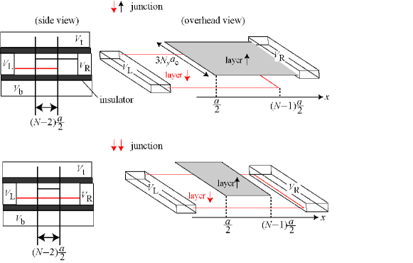
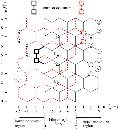
We consider the two kinds of po-G, $\downarrow\uparrow$ and $\downarrow\downarrow$, as shown in Fig. 1, where $\downarrow$ and $\uparrow$ denote the lower and upper graphene layers, respectively. The top $V_{\rm t}$ and bottom $V_{\rm b}$ gate electrodes exert a vertical electric field on the two layers. The bilayer region is limited spatially and each of the bias electrodes $V_{\rm L}$ and $V_{\rm R}$ connects with only one of the layers. In the $\downarrow\uparrow$ junction, $V_{\rm L}$ and $V_{\rm R}$ connect with the $\downarrow$ and $\uparrow$ layers, respectively. In the $\downarrow\downarrow$ junction, both $V_{\rm L}$ and $V_{\rm R}$ connect with the $\downarrow$ layer. Figure 2 shows the atomic structures of the $\downarrow\uparrow$ junction in the case of $N=6$. The dotted and solid lines represent $\downarrow$ and $\uparrow$ layers, respectively. Integer indexes ($j$, $j_{y}$) and sublattice indexes $(A,B)$ specify the atomic coordinates $(x,y)$ as $x=\frac{a}{2}j$, $y_{\rm A,\downarrow}=y_{\rm A,\uparrow}=3a_{\rm c}[j_{y}+\frac{1+(-1)^{j}}{4}]$, $y_{\rm B,\downarrow}=y_{\rm A}-a_{\rm c}$, and $y_{\rm B,\uparrow}=y_{\rm A}+a_{\rm c}$ with the lattice constant $a$ and the bond length $a_{\rm c}=a/\sqrt{3}$. The bilayer region is limited in the range $1\leq j\leq N-1$ with the geometrical overlap length $(N-2)a/2$. The left $j\leq 0$ and right $N\leq j$ monolayer regions respectively correspond to the $\downarrow$ and $\xi$ layers in the $\downarrow\xi$ junction ($\xi=\downarrow,\uparrow)$. Bonded squares denote carbon dimers added to armchair edges. The addimer $(x,y)$ positions are represented by $(0,(3m+2)a_{\rm c})$ and $(Na/2,(3m^{\prime}+1)a_{\rm c})$ with integers $m$ and $m^{\prime}$. When not explicitly noted, we assume the perfect armchair edges.

Figure 1: (Color online) Arrangements of electrodes and graphene layers $\downarrow$ and $\uparrow$. $V_{\rm t}$ and $V_{\rm b}$ denote the top and bottom gate electrodes, respectively. $V_{\rm L}$ and $V_{\rm R}$ denote the bias electrodes.

Figure 2: (Color online) Indexes $j,j_{y},A,$ and $B$ and atomic positions in the $\downarrow\uparrow$ junction. Layers $\downarrow$ and $\uparrow$ are parallel to the $xy$ plane.

The wave functions at sublattices A and B are represented by $A_{\xi,j,j_{y}}$ and $B_{\xi,j,j_{y}}$ with the layer index $\xi=\downarrow,\uparrow$. Using the periodic boundary condition $(A,B)_{j_{y}+N_{y}}=(A,B)_{j_{y}}$ with the transverse width $3N_{y}a_{\rm c}$, we can reduce the dimension of the TB equations of the bilayer region as

$$E\vec{c}_{\downarrow,j} = (h_{0}-\varepsilon)\vec{c}_{\downarrow,j}+h_{1}\left(\vec{c}_{\downarrow,j-1}+\vec{c}_{\downarrow,j+1}\right)$$ (1)

$$+W_{0}\vec{c}_{\uparrow,j}+W_{1}\left(\vec{c}_{\uparrow,j-1}+\vec{c}_{\uparrow,j+1}\right),$$

$$E\vec{c}_{\uparrow,j} = (h_{0}+\varepsilon)\vec{c}_{\uparrow,j}+h_{1}^{*}\left(\vec{c}_{\uparrow,j-1}+\vec{c}_{\uparrow,j+1}\right)$$ (2)

$$+W_{0}^{*}\vec{c}_{\downarrow,j}+W_{1}^{*}\left(\vec{c}_{\downarrow,j-1}+\vec{c}_{\downarrow,j+1}\right),$$

where

$$\;{}^{t}\vec{c}_{\xi,j}=e^{-\frac{i}{2}\kappa\left[(-1)^{j}+1\right]}(A_{\xi,j,0},B_{\xi,j,0}),$$ (3)

$$h_{0}=\gamma_{0}\left(\begin{array}[]{cc}0&1\\ 1&0\end{array}\right),\;\;h_{1}=\gamma_{0}\left(\begin{array}[]{cc}0&e^{i\kappa}\\ e^{-i\kappa}&0\end{array}\right),$$ (4)

$$W_{0}=\left(\begin{array}[]{cc}\gamma_{1}&\gamma_{4}\\ \gamma_{4}&\gamma_{3}e^{-2i\kappa}\end{array}\right),\;W_{1}=e^{-i\kappa}\left(\begin{array}[]{cc}0&\gamma_{4}\\ \gamma_{4}&\gamma_{3}\end{array}\right),$$ (5)

$\kappa=\frac{\sqrt{3}}{2}k_{y}a$, and $k_{y}$ is the $y$ component of the wave number vector. The vertical electric field induces the interlayer difference $2\varepsilon$ in site energy [103]. Two kinds of TB models, $\gamma_{1}\gamma_{3}\gamma_{4}$-TB and $\gamma_{1}$-TB models, are used, where the latter is an approximation of the former. According to Ref. [104] , the $\gamma_{1}\gamma_{3}\gamma_{4}$-TB parameters are $\gamma_{0}=-3.12$ eV , $\gamma_{1}=0.377$ eV, $\gamma_{3}=0.29$ eV, and $\gamma_{4}=0.12$ eV. The $\gamma_{1}$-TB parameters are the same as the $\gamma_{1}\gamma_{3}\gamma_{4}$-TB parameters except that $\gamma_{3}=\gamma_{4}=0$. The Hamiltonian elements of the addimers are defined in the same way.

Applying the exact method in Ref. [105] to Eqs. (1) and (2), we can calculate $T_{\nu^{\prime},\nu}(\kappa)$ that denotes the transmission rate from the left $K_{\nu}$ state to the right $K_{\nu^{\prime}}$ state. The Landauer’s formula conductivity $g$ (conductance per width $3a_{\rm c}$ in the unit of 2$e^{2}/h$ ) and the absolute VCR conductivity $g_{\rm v}$ are represented by

$$\left(\begin{array}[]{l}g\\ g_{\rm v}\end{array}\right)=\frac{1}{N_{y}}\sum_{m=-M}^{M}\left(\begin{array}[]{l}g^{\prime}(m\Delta\kappa)\\ g_{\rm v}^{\prime}(m\Delta\kappa)\end{array}\right),$$ (6)

where

$$\left(\begin{array}[]{l}g^{\prime}(\kappa)\\ g_{\rm v}^{\prime}(\kappa)\end{array}\right)=\sum_{\nu=\pm}\sum_{\nu^{\prime}=\pm}\left(\begin{array}[]{l}1\\ \frac{-\nu\nu^{\prime}}{2}\end{array}\right)T_{\nu^{\prime},\nu}(\kappa).$$ (7)

The relative VCR conductivity is represented by $g_{\rm v}/g$. Owing to the periodic boundary condition with the period $3N_{y}a_{\rm c}$, the transverse wave number $k_{y}$ is discrete as $k_{y}=m\frac{2\pi}{3N_{y}a_{\rm c}}$ with integers $m$. As $\kappa=\frac{\sqrt{3}}{2}k_{y}a$, the interval of the discrete $\kappa$ is represented by $\Delta\kappa=\frac{\sqrt{3}}{2}a\Delta k_{y}=\frac{\pi}{N_{y}}$. The wave number vector $\vec{k}=(k_{x},k_{y})$ of the monolayer region must satisfy the dispersion relation

$$\frac{(E\pm\varepsilon)^{2}}{\gamma_{0}^{2}}=\left(2\cos\left(\frac{a}{2}k_{x}\right)+\cos\kappa\right)^{2}+\sin^{2}\kappa$$ (8)

indicating the energy gap $|E\pm\varepsilon|\leq|\gamma_{0}\sin\kappa|$ in a subband with a fixed $\kappa$. The integer $M$ in Eq. (6) corresponds to the maximum of the allowed $|k_{y}|$ and is represented by

$$M=\left\{\begin{array}[]{l}{\rm Int}\left[\frac{N_{y}}{\pi}\arcsin\left|\frac{|E|-|\varepsilon|}{\gamma_{0}}\right|\right]\;\;\cdots(\downarrow\uparrow\;{\rm junction})\\ {\rm Int}\left[\frac{N_{y}}{\pi}\arcsin\left|\frac{E+\varepsilon}{\gamma_{0}}\right|\right]\;\;\cdots(\downarrow\downarrow\;{\rm junction})\end{array}\right.,$$ (9)

where Int$[x]$ denotes the maximum integer that does not exceed $x$. The average VCR transmission rate for the active $2M+1$ subbands is represented by

$$\widetilde{g}_{\rm v}=\frac{N_{y}}{2M+1}g_{\rm v}$$ (10)

that is relevant to both $g_{\rm v}$ and $g_{\rm v}/g$. When $\widetilde{g}_{\rm v}=1$, the VCR transmission rates become perfect for both $T_{+,-}$ and $T_{-,+}$ in all the $2M+1$ subbands. It follows that $g_{\rm v}$ and $g_{\rm v}/g$ concurrently reach their upper limits, $(2M+1)/N_{y}$ and $\frac{1}{2}$. Under the condition $\tilde{g}_{\rm v}=1$, the pure VC changes into the inverse pure VC without losing its intensity. The condition $T_{+,-}=T_{-,+}$, which follows the condition $\widetilde{g}_{\rm v}=1$, is necessary for this pure VCR. When only one of $T_{+,-}$ or $T_{-,+}$ reaches one, a pure VC changes into a nonpure VC. Even when the relative VCR conductivity is perfect ($g_{\rm v}/g=\frac{1}{2}$), the absolute VCR conductivity may be far from the upper limit ($g_{\rm v}\ll(2M+1)/N_{y}$). Inversely, $g_{\rm v}$ may be large with a small $g_{\rm v}/g$ owing to a large $M/N_{y}$. The condition $\widetilde{g}_{\rm v}\simeq 1$ rules out these cases where only one of $g_{\rm v}/g$ or $g_{\rm v}$ is large. Refer to Appendix A for the detailed VC formulas.

The signs of $\gamma_{0}$ and $\gamma_{4}$ are reversed compared with those shown in Ref. [104] by the transformation $(A^{\prime},B^{\prime})=(A,-B)$. The transformation $(A^{\prime}_{\downarrow},B^{\prime}_{\downarrow})=(A_{\downarrow},-B_{\downarrow}),$ $(A^{\prime}_{\uparrow},B^{\prime}_{\uparrow})=(-A_{\uparrow},B_{\uparrow})$ proves that the $\gamma_{1}$-TB model has the symmetry

$$\tilde{g}_{\rm v}(E,\varepsilon)=\tilde{g}_{\rm v}(-E,-\varepsilon)$$ (11)

for both the $\downarrow\uparrow$ and $\downarrow\downarrow$ junctions. Even in the $\gamma_{1}\gamma_{3}\gamma_{4}$-TB model, Eq. (11) holds approximately. Refer to Ref. [105] for this insignificance of $\gamma_{3}$ and $\gamma_{4}$. Appendix A proves that the $\downarrow\uparrow$ junction satisfies

$$\tilde{g}_{\rm v}(E,\varepsilon)=\tilde{g}_{\rm v}(E,-\varepsilon)$$ (12)

in both the $\gamma_{1}$-TB and $\gamma_{1}\gamma_{3}\gamma_{4}$-TB models, whereas Eq. (12) is invalid for the $\downarrow\downarrow$ junction. Owing to Eq. (11) that holds approximately (exactly) in the $\gamma_{1}\gamma_{3}\gamma_{4}$-TB ($\gamma_{1}$-TB) model, we eliminate the negative $\varepsilon$ from the rest of this paper.

	$\frac{dE}{dk}>0\;\;(p=+)$		$\frac{dE}{dk}<0\;\;(p=-)$
	$K_{+}$	$K_{-}$	$K_{+}$	$K_{-}$
bilayer	$k_{l}^{(+)}$	$-k_{l}^{(-)}$	$k_{l}^{(-)}$	$-k_{l}^{(+)}$
$l=+,-$
monolayer	$k_{\xi}^{(+)}$	$-k_{\xi}^{(-)}$	$k_{\xi}^{(-)}$	$-k_{\xi}^{(+)}$
$\xi=\downarrow,\uparrow$
	$K_{+}$
$E>0$	$k_{+}^{(\sigma)}\simeq k^{(\sigma)}_{\downarrow},\;\;k_{-}^{(\sigma)}\simeq k^{(\sigma)}_{\uparrow}$
$E<0$	$k_{+}^{(\sigma)}\simeq k^{(\sigma)}_{\uparrow},\;\;k_{-}^{(\sigma)}\simeq k^{(\sigma)}_{\downarrow}$

Table 1: Relation of the indexes $l,\sigma$ to the layers $\xi=\downarrow,\uparrow$, the sign of the group velocity $p=\frac{dE}{dk}/\left|\frac{dE}{dk}\right|$, and the valleys $K_{\pm}$.

3 $\gamma_{1}$-TB Calculation of Zero Lateral Wave Number

In Sect. 3, we discuss the $\gamma_{1}$-TB calculation of subband $\kappa=0$. Figure 3 exemplifies the wave number $k_{l}^{(\sigma)}$ at the $K_{+}$ valley with sign indexes $l=\pm$ and $\sigma=\pm$. At the other valley $K_{-}$, $k=-k^{(\sigma)}_{l}\simeq-4\pi/(3a)$. The group velocity $\frac{dE}{dk}$ at the $K_{+}$ valley is positive (negative) when $\sigma=+$ $(\sigma=-)$. For the positive (negative) group velocity states, the index $\sigma$ corresponds to the $K_{\sigma}$ ($K_{-\sigma})$ valley. The index $l$ is assigned according to the condition $\left|k^{(\sigma)}_{+}-4\pi/(3a)\right|\geq\left|k^{(\sigma)}_{-}-4\pi/(3a)\right|$. When $lE$ is positive (negative), the $k_{l}$ dispersion line is similar to the monolayer $\downarrow$ ($\uparrow$) dispersion line. In this sense, the index $l$ is the roots layer index. Table I summarizes the physical meaning of the indexes $l$ and $\sigma$. Figure 3 also demonstrates the bilayer propagating mode number $N_{\downarrow\uparrow}$ at each valley as

$$N_{\downarrow\uparrow}=\left\{\begin{array}[]{l}0\;\;\;\cdots|E|<\Delta\;\;\;({\rm gap)}\\ 4\;\;\;\cdots\Delta<|E|<\varepsilon\;\;\;({\rm inner\;\;}E)\\ 2\;\;\;\cdots\varepsilon<|E|<\Delta^{\prime}\;\;\;({\rm pseudogap)}\\ 4\;\;\;\cdots\Delta^{\prime}<|E|\;\;\;({\rm outer\;\;}E)\end{array}\right.$$ (13)

with the gap edge $\Delta=\frac{\gamma_{1}\varepsilon}{\sqrt{4\varepsilon^{2}+\gamma_{1}^{2}}}$ and the upper pseudogap edge $\Delta^{\prime}=\sqrt{\varepsilon^{2}+\gamma_{1}^{2}}$ [106, 107, 108, 109] .

Figure 3: Dispersion relation of the bilayer region calculated using the $\gamma_{1}$-TB model for $\varepsilon=$ 0.35 eV and $\kappa=0$.

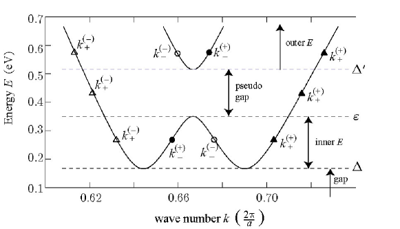
The gap and pseudogap regions are excluded in Sect. 3, as their smaller mode number suppresses the conductivity. In Sect. 3.1, we explain the exact formulas of the inner and outer $E$ regions. Refer to Ref. [105] for the exact calculation method of the gap and pseudogap regions. In Sects. 3.2 and 3.3, $k_{l}^{(\sigma)}$ approximates $\frac{4\pi}{3a}$ in the scattering between the monolayer and bilayer regions. In Sect. 3.3, we neglect the difference between $\left|k_{l}^{(+)}-\frac{4\pi}{3a}\right|$ and $\left|k_{l}^{(-)}-\frac{4\pi}{3a}\right|$ in the propagation through the bilayer region. The transmission rate is concisely expressed in Sect. 3.3 when $N$ is a multiple of three. This expression is interpreted according to the wave function nature. Except when $\downarrow\downarrow$ is explicitly referred to, in Sect. 3, we mainly discuss the $\downarrow\uparrow$ junction. It is straightforward to derive the $\downarrow\downarrow$ formulas from the $\downarrow\uparrow$ formulas.

3.1 Exact calculations

The dispersion relation and wave function of the bilayer region are represented by

$$\cos\left(\frac{a}{2}k^{(\sigma)}_{l}\right)=\frac{-1}{2}\left(1+l\sigma\sqrt{3}\theta_{l}\right),$$ (14)

$$\left(\begin{array}[]{c}\vec{c}_{\downarrow,j}\\ \vec{c}_{\uparrow,j}\end{array}\right)=\sum_{\sigma=\pm}\sum_{l=\pm}\sum_{p=\pm}\frac{\omega_{\sigma,l}^{pj}}{\sqrt{J_{\sigma,l}}}\eta^{(p)}_{\sigma,l}\left(\begin{array}[]{c}\vec{d}^{\;\downarrow}_{\sigma,l}\\ \vec{d}^{\;\uparrow}_{\sigma,l}\end{array}\right),$$ (15)

where $\eta$ denotes the mode amplitude, $\omega_{\pm,l}=e^{\pm i\frac{a}{2}k_{l}^{(\pm)}}$,

$$\left[\;{}^{t}\vec{d}_{\sigma,l}^{\;\downarrow},\;^{t}\vec{d}_{\sigma,l}^{\;\uparrow}\right]=\left[(\sigma l\alpha_{l},\;1),\;\beta_{l}\left(\sigma l\alpha_{l}\frac{E-\varepsilon}{E+\varepsilon},\;1\right)\right],$$ (16)

$$J_{\sigma,l} = \sum_{\xi=\downarrow,\uparrow}{\rm Im}\left[w^{*}_{\sigma,l}\!{}^{t}\vec{d}_{\sigma,l}^{\;\xi}h_{1}\vec{d}_{\sigma,l}^{\;\xi}\right]$$ (17)

$$= 2|\gamma_{0}|v_{l}\sin\left(\frac{a}{2}k_{l}^{(\sigma)}\right),$$

$$v_{l}=\frac{\alpha_{l}}{\beta_{(-l)}}\left(\beta_{-}-\beta_{+}\right),$$ (18)

$$\beta_{l}=\frac{2\varepsilon E-l\sqrt{(\gamma_{1}^{2}+4\varepsilon^{2})E^{2}-\gamma_{1}^{2}\varepsilon^{2}}}{\gamma_{1}(E-\varepsilon)},$$ (19)

$$\alpha_{l}=\frac{E+\varepsilon}{\sqrt{3}|\gamma_{0}|\theta_{l}},$$ (20)

$$\theta_{l}=\tau_{l}\frac{E}{|E|}\frac{\sqrt{E^{2}+\varepsilon^{2}+l\sqrt{(\gamma_{1}^{2}+4\varepsilon^{2})E^{2}-\gamma_{1}^{2}\varepsilon^{2}}}}{\sqrt{3}|\gamma_{0}|},$$ (21)

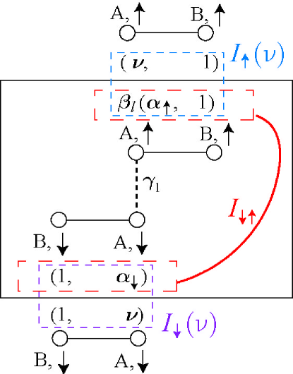
where $\tau_{\pm}=1$ ($\tau_{\pm}=\pm 1$ ) in the inner (outer) $E$ [106, 107, 108, 109]. The solid square area of Fig. 4 shows the spatial arrangement of elements of Eq. (16), where $\alpha_{\downarrow}=\sigma l\alpha_{l}$ and $\alpha_{\uparrow}=\alpha_{\downarrow}(E-\varepsilon)/(E+\varepsilon)$. When there is a single mode such as $(\vec{c}_{\downarrow,j},\vec{c}_{\uparrow,j})=w_{\sigma,l}^{j}(\vec{d}_{\sigma,l}^{\;\downarrow},\vec{d}_{\sigma,l}^{\;\uparrow})$, the probability flow equals $J_{\sigma,l}$. Here, we have chosen the definitions as conditions $v_{l}>0$ and $J_{\sigma,l}>0$ hold. The probability flow of Eq. (15) is the same as $\sum_{l,\sigma}|\eta^{(+)}_{l,\sigma}|^{2}-|\eta^{(-)}_{l,\sigma}|^{2}$, indicating that the sign $p=\pm$ denotes the propagation direction. In the same way as the bilayer region, the dispersion relation and wave function of each monolayer region are represented by

$$\cos\left(\frac{a}{2}k^{(\nu)}_{\;{}_{\uparrow}^{\downarrow}}\right)=\frac{-1}{2}\left(1+\nu\frac{E\pm\varepsilon}{|\gamma_{0}|}\right),$$ (22)

$$\vec{c}_{\downarrow,j}^{\;(0)}=\sum_{\nu=\pm}\sum_{p=\pm}\frac{\omega_{\nu,\downarrow}^{pj}}{\sqrt{J_{\nu,\downarrow}}}\eta^{(p)}_{\nu,{\rm L}}\left(\begin{array}[]{c}\nu\\ 1\end{array}\right),$$ (23)

$$\vec{c}_{\uparrow,j}^{\;(0)}=\sum_{\nu=\pm}\sum_{p=\pm}\frac{\omega_{\nu,\uparrow}^{p(j-N)}}{\sqrt{J_{\nu,\uparrow}}}\eta^{(p)}_{\nu,{\rm R}}\left(\begin{array}[]{c}\nu\\ 1\end{array}\right),$$ (24)

where $\omega_{\pm,\xi}=e^{\pm i\frac{a}{2}k_{\xi}^{(\pm)}}$,

$$J_{\nu,\xi}=2|\gamma_{0}|\sin\left(\frac{a}{2}k_{\xi}^{(\nu)}\right)$$ (25)

with the layer index $\xi=\downarrow,\uparrow$. The superscript (0) in Eqs. (23) and (24) indicates that there is no interlayer transfer integral. Each coefficient $\eta$ of Eq. (15) [Eqs. (23) and (24)] corresponds to the $K_{p\sigma}$ [$K_{p\nu}$] valley . The top and bottom of Fig. 4 show amplitudes of single layer modes in the $\downarrow\uparrow$ junction.

Figure 4: (Color online) Cross-sectional view of elements of Eqs. (15), (23), and (24), where $\alpha_{\downarrow}=\sigma l\alpha_{l}$ and $\alpha_{\uparrow}=\alpha_{\downarrow}(E-\varepsilon)/(E+\varepsilon)$. Refer to the main text about the interlayer matching $I_{\downarrow\uparrow}$ and monolayer–bilayer matching $I_{\xi}(\nu)$ where $\xi=\downarrow,\uparrow$.

The scattering matrixes $S_{\downarrow}$ and $S_{\uparrow}$ are defined by

$$\left(\begin{array}[]{c}\vec{\eta}^{\;(+)}\\ \vec{\eta}^{\;(-)}_{\rm L}\end{array}\right)=S_{\downarrow}\left(\begin{array}[]{c}\vec{\eta}^{\;(-)}\\ \vec{\eta}^{\;(+)}_{\rm L}\end{array}\right),$$ (26)

$$\left(\begin{array}[]{c}\Lambda^{*}\vec{\eta}^{\;(-)}\\ \vec{\eta}^{\;(+)}_{\rm R}\end{array}\right)=S_{\uparrow}\left(\begin{array}[]{c}\Lambda\vec{\eta}^{\;(+)}\\ \vec{\eta}^{\;(-)}_{\rm R}\end{array}\right),$$ (27)

where $\;{}^{t}\vec{\eta}^{\;(p)}=(\eta_{+,+}^{(p)},\;\eta_{-,+}^{(p)},\;\eta_{+,-}^{(p)},\;\eta_{-,-}^{(p)})$, $\;{}^{t}\vec{\eta}^{\;(p)}_{\rm L}=(\eta_{+,{\rm L}}^{(p)},\;\eta_{-,{\rm L}}^{(p)})$, $\;{}^{t}\vec{\eta}^{\;(p)}_{{\rm R}}=(\eta_{+,{\rm R}}^{(p)},\;\eta_{-,{\rm R}}^{(p)})$ and

$$\Lambda_{(\sigma,l|\sigma^{\prime},l^{\prime})}=\delta_{\sigma,\sigma^{\prime}}\delta_{l,l^{\prime}}e^{\sigma i\frac{a}{2}Nk_{l}^{(\sigma)}}.$$ (28)

The boundary conditions are

$$(\vec{c}_{\downarrow,0},\vec{c}_{\uparrow,0},\vec{c}_{\downarrow,1})=(\vec{c}_{\downarrow,0}^{\;(0)},0,\vec{c}_{\downarrow,1}^{\;(0)})$$ (29)

for $S_{\downarrow}$ and

$$(\vec{c}_{\uparrow,N},\vec{c}_{\downarrow,N},\vec{c}_{\uparrow,N-1})=(\vec{c}_{\uparrow,N}^{\;(0)},0,\vec{c}_{\uparrow,N-1}^{\;(0)})$$ (30)

for $S_{\uparrow}$. The exact $S_{\downarrow}$ and $S_{\uparrow}$ follow from the application of Eqs. (15), (23), and (24) to Eqs. (29) and (30). Eliminating $\eta^{(\pm)}$ from Eqs. (26) and (27), we obtain

$$t_{\uparrow\downarrow}=\;^{t}t_{\uparrow}\Lambda\left({\bf 1}_{4}-r_{\downarrow}\Lambda r_{\uparrow}\Lambda\right)^{-1}t_{\downarrow},$$ (31)

which satisfies $\vec{\eta}^{\;(+)}_{\rm R}=t_{\uparrow\downarrow}\vec{\eta}^{\;(+)}_{\rm L}$, where $r_{\xi}$ ($t_{\xi}$) and ${\bf 1}_{n}$ denote the $S_{\xi}$ reflection (transmission) block and the $n$ dimensional unit matrix, respectively. The transmission rate $T_{\nu^{\prime},\nu}(0)$ equals the squared absolute value of the element of $t_{\uparrow\downarrow}$. Replacing $\uparrow$ with $\downarrow$ in Eq. (31), we obtain $T_{\nu^{\prime},\nu}$ of the $\downarrow\downarrow$ junction.

3.2 First approximation

The approximation $k_{\pm}^{(\sigma)}\simeq k_{\downarrow}^{(\sigma)}\simeq\frac{4\pi}{3a}$ simplifies Eq. (29) to

$$X_{\downarrow}\left(\begin{array}[]{c}\vec{\eta}^{\;(+)}\\ \vec{\eta}^{\;(-)}_{\rm L}\end{array}\right)=-X_{\downarrow}^{*}\left(\begin{array}[]{c}\vec{\eta}^{\;(-)}\\ \vec{\eta}^{\;(+)}_{\rm L}\end{array}\right),$$ (32)

where

$$X_{\downarrow}=\left(\begin{array}[]{ccc}u_{+}^{\downarrow}&u_{-}^{\downarrow}&-u_{0}\\ u_{+}^{\uparrow}&u_{-}^{\uparrow}&0\\ u_{+}^{\downarrow}\Omega&u_{-}^{\downarrow}\Omega&-u_{0}\Omega^{*}\end{array}\right),$$ (33)

$$u_{l}^{\xi}=\frac{1}{\sqrt{v_{l}}}(\vec{d}_{+,l}^{\;\xi},\vec{d}_{-,l}^{\;\xi}),\;\;u_{0}=\left(\begin{array}[]{cc}1&-1\\ 1&1\end{array}\right),$$ (34)

$$\Omega=\left(\begin{array}[]{cc}e^{i\frac{2}{3}\pi}&0\\ 0&e^{-i\frac{2}{3}\pi}\end{array}\right).$$ (35)

Using the Kronecker product, we present $S_{\downarrow}=-X_{\downarrow}^{-1}X_{\downarrow}^{*}$ as

$$S_{\downarrow}=Y_{B}\;^{t}Y_{B}\otimes u_{B}+Y_{A}\;^{t}Y_{A}\otimes u_{A}-{\bf 1}_{6},$$ (36)

where

$$Y_{B}=\sqrt{\frac{2}{c_{B}}}\left(\begin{array}[]{cc}\frac{\alpha_{+}}{\sqrt{v_{+}}}\\ -\frac{\alpha_{-}}{\sqrt{v_{-}}}\\ 1\end{array}\right),\;Y_{A}=\sqrt{\frac{2}{c_{A}}}\left(\begin{array}[]{cc}\frac{1}{\sqrt{v_{+}}}\\ \frac{1}{\sqrt{v_{-}}}\\ 1\end{array}\right),$$ (37)

$$u_{\;{}_{A}^{B}}=\;\frac{1}{2}\left(\begin{array}[]{cc}1&\pm 1\\ \pm 1&1\end{array}\right),$$ (38)

$$c_{\;{}_{A}^{B}}=1+\frac{\alpha_{+}^{\pm 1}\beta_{-}+\alpha_{-}^{\pm 1}\beta_{+}}{\beta_{-}-\beta_{+}}.$$ (39)

We can easily confirm that Eq. (36) satisfies relation $X_{\downarrow}S_{\downarrow}=-X_{\downarrow}^{*}$. We also obtain an approximate formula

$$S_{\uparrow}=VS^{\prime}_{\downarrow}V,$$ (40)

where

$$V=\left(\begin{array}[]{ccc}\frac{\beta_{+}}{|\beta_{+}|}{\bf 1}_{2}&0&0\\ 0&\frac{\beta_{-}}{|\beta_{-}|}{\bf 1}_{2}&0\\ 0&0&{\bf 1}_{2}\end{array}\right),$$ (41)

and we transform $S_{\downarrow}$ into $S^{\prime}_{\downarrow}$ by replacing $(\alpha_{l},\beta_{l})$ with $(\alpha_{l}^{\prime},\beta_{l}^{\prime})=\left(\frac{E-\varepsilon}{E+\varepsilon}\alpha_{l},\frac{1}{\beta_{l}}\right)$. Equations (36) and (40) satisfy the unitary condition $\!{}^{t}S_{\downarrow}^{*}S_{\downarrow}=\!^{t}S_{\uparrow}^{*}S_{\uparrow}={\bf 1}_{6}$. The calculation of $T_{\nu^{\prime},\nu}(0)$ with Eqs. (28), (31), (36), and (40) is referred to as the first approximation.

3.3 Second approximation

Figure 3 and Eq. (14) demonstrate that $\frac{a}{2}k_{l}^{(\pm)}\simeq\frac{2\pi}{3}\pm l\theta_{l}$. This leads to an approximation that replaces Eq. (28) as follows:

$$\Lambda_{(\sigma,s|\sigma^{\prime},s^{\prime})}=\delta_{\sigma,\sigma^{\prime}}\delta_{s,s^{\prime}}\exp\left[iN\left(\sigma\frac{2}{3}\pi+l\theta_{l}\right)\right].$$ (42)

When $N/3$ is an integer, the phase $2\sigma\pi N/3$ of Eq. (42) has no effect. This simplifies Eq. (31) to

$$t_{\uparrow\downarrow}=\sum_{\chi=A,B}\;^{t}t_{\uparrow,\chi}\tilde{\Lambda}\left({\bf 1}_{2}-r_{\downarrow,\chi}\tilde{\Lambda}r_{\uparrow,\chi}\tilde{\Lambda}\right)^{-1}t_{\downarrow,\chi}\otimes u_{\chi},$$ (43)

where

$$\tilde{\Lambda}=\left(\begin{array}[]{cc}e^{i\theta_{+}N}&0\\ 0&e^{-i\theta_{-}N}\end{array}\right).$$ (44)

See Sect. 3.2 for the definitions of the $t_{\xi,\chi}$ and $r_{\xi,\chi}$ matrixes. For example, $\;{}^{t}t_{\downarrow,A}=\frac{2}{c_{A}}\left(\frac{1}{\sqrt{v_{+}}},\frac{1}{\sqrt{v_{-}}}\right)$ and $r_{\downarrow,A}=\frac{c_{A}}{2}t_{\downarrow,A}\;^{t}t_{\downarrow,A}-{\bf 1}_{2}$. The relation $u_{\chi}u_{\chi^{\prime}}=\delta_{\chi,\chi^{\prime}}u_{\chi}$ and Eq. (43) bring us the second approximation

$$T_{\nu^{\prime},\nu}=\left|\frac{G_{B}}{F_{B}}+\nu\nu^{\prime}\frac{G_{A}}{F_{A}}\right|^{2}.$$ (45)

See Appendix B for explicit expressions of $G$ and $F$. Note that the second approximation (45) is valid only when $N/3$ is an integer.

Here, we introduce

$$q\equiv\left(\frac{2\varepsilon}{\gamma_{1}}\right)^{2}.$$ (46)

When $|E|$ approaches the gap edge $\Delta$, $|\theta_{\pm}|$ converges to $\theta_{0}$, where

$$\theta_{0}=\frac{\gamma_{1}}{2\sqrt{3}|\gamma_{0}|}\sqrt{\frac{q(2+q)}{1+q}}.$$ (47)

At the gap edge $|E|=\Delta$,

$$\left(T_{\pm,\pm},T_{\pm,\mp}\right)\simeq\frac{q}{1+q}\left(\frac{\sin^{2}(\theta_{0}N)}{\theta_{0}^{2}N^{2}},\;\cos^{2}(\theta_{0}N)\right)$$ (48)

holds in the $N$ range

$$\frac{\sqrt{(2+q)^{3}}}{(2+2q)\theta_{0}}\ll N\ll 2\frac{\sqrt{2+q}}{\theta_{0}}.$$ (49)

This suggests that

$$g^{\prime}_{\rm v}(0)\simeq\frac{q}{1+q}$$ (50)

when conditions (49),

$$N\simeq\pi/\theta_{0},$$ (51)

and $|E|\simeq\Delta$ hold. The exact $g^{\prime}_{\rm v}(0)$ peak certainly appears under conditions (49), (51), and

$$|E|\simeq\frac{\Delta}{3}\sqrt{11+q}$$ (52)

with the height of about $q/(1+q)$. Appendix B shows that Eq. (51) requires the condition $q<8$. As $|E|$ increases from $\Delta$ to Eq. (52) with $N$ fixed to Eq. (51), $N(|\theta_{+}|+|\theta_{-}|)/2$ remains about $\pi$, whereas the difference between $\pi$ and $N|\theta_{\pm}|$ increases from near zero to about $\pi/3$.

When $|E|\gg\sqrt{4\varepsilon^{2}+\gamma_{1}^{2}}$, Eq. (45) approximates

$$T_{\pm,\pm}\simeq\frac{(s_{+}-s_{-})^{2}}{\left|F^{\prime}\right|^{2}(1+q)},\;\;T_{\pm,\mp}\simeq\frac{\gamma_{1}^{2}(s_{+}+s_{-})^{2}}{4\left|F^{\prime}\right|^{2}E^{2}},$$ (53)

where $s_{\pm}=\sin(|\theta_{\pm}|N)$ and

$$F^{\prime}=\frac{-1}{1+q}\sin^{2}\left(\frac{|\theta_{+}|-|\theta_{-}|}{2}N\right)-e^{i(|\theta_{+}|+|\theta_{-}|)N}.$$ (54)

Refer to Appendix B for the derivation. The second approximate $T_{\pm,\mp}$ formula of the $\downarrow\downarrow$ junction (not shown here explicitly) also becomes proportional to $E^{-2}$ when $|E|\gg\sqrt{4\varepsilon^{2}+\gamma_{1}^{2}}$.

The second approximation is closely related to another expression of Eq. (15),

$$\left(\begin{array}[]{c}\vec{c}_{\downarrow,j}\\ \vec{c}_{\uparrow,j}\end{array}\right)=\sum_{\chi=A,B}\sum_{l=\pm}\sum_{p=\pm}\frac{e^{ilp\theta_{l}j}}{\sqrt{\sqrt{3}|\gamma_{0}|v_{l}}}\zeta^{(p)}_{\chi,l}\vec{f}^{\;(p)}_{\chi,l,j},$$ (55)

where

$$\left(\vec{f}_{B,l,j}^{\;(\pm)},\vec{f}_{A,l,j}^{\;(\pm)}\right)=\left(\begin{array}[]{cc}0&\alpha_{l}\\ 1&0\\ 0&\beta_{l}\alpha_{l}^{\prime}\\ \beta_{l},&0\end{array}\right)\left(\begin{array}[]{cc}c_{j}&\pm is_{j}\\ \pm ils_{j}&lc_{j}\end{array}\right),$$ (56)

$\zeta_{\;{}_{A}^{B},l}^{(p)}=\eta_{+,l}^{(p)}\pm\eta_{-,l}^{(p)}$, $c_{j}=\cos(2\pi j/3)$, and $s_{j}=\sin(2\pi j/3)$. Equations (55) and (56) possess two important characteristics. First, mode $\zeta_{\chi,l}^{(p)}$ is a Bloch state with the unit cell length $3a/2$ and the wave number $2pl\theta_{l}/a$. Second, $\vec{f}_{\chi,l,j}^{\;(p)}$ is localized at the $\chi$ site when $j/3$ is an integer. These characteristics explain the interference between the $\vec{f}_{A}$ and $\vec{f}_{B}$ modes in Eq. (45).

4 Results

4.1 $\downarrow\uparrow$ junction

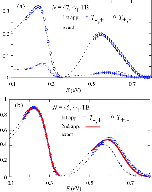
Crosses and circles in Fig. 5 represent the first approximations of $T_{-,+}(0)$ and $T_{+,-}(0)$, respectively. The longitudinal overlap lengths are $N=47$ in Fig. 5(a) and $N=45$ in Fig. 5(b). The solid line in Fig. 5(b) shows the second approximation of $T_{\pm,\mp}$. As the second approximation is irrelevant to a non-integer $N/3$, the solid line does not appear in Fig. 5(a). These approximation results reproduce well the exact $T_{+,-}(0)$ and $T_{-,+}(0)$ displayed by the dashed lines. Unlike the exact calculation, the approximate formulas are not available in the gap and pseudogap energy regions. However, these energy regions are unimportant because of their low transmission rate. As Fig. 5 shows, the difference between $T_{+,-}(0)$ and $T_{-,+}(0)$ is smaller with an integer $N/3$ than with a non-integer $N/3$. It follows that an integer $N/3$ is advantageous for the $g^{\prime}_{\rm v}(0)$ to reach the upper limit. In the $\gamma_{1}\gamma_{3}\gamma_{4}$-TB model, Eq. (12) is exact, whereas Eq. (11) is approximate; thus, the relation $\tilde{g}_{\rm v}(E,\varepsilon)=\tilde{g}_{\rm v}(-E,\varepsilon)$ does not exactly hold. The numerical results show that the $\tilde{g}_{\rm v}$ peak is slightly higher in the negative $E$ region than in the positive $E$ region. As high $\tilde{g}_{\rm v}$ is our concern, the figures in this paper, except for Figs. 3 and 5, display data on an integer $N/3$ and negative $E$.

Figure 5: (Color online) VCR transmission rate $T_{\pm,\mp}$ calculated using the $\gamma_{1}$-TB model in the case of $\kappa=0$, $\varepsilon=$ 0.35 eV, (a) $N=47$, and (b) $N=45$.

Figure 6: (Color online) VCR data of the $\downarrow\uparrow$ junction in the case of $\varepsilon=0.35$ eV, $N_{y}=1000$, and $N=45,48,51,54,$ and 57. Blue lines in the left and right panels represent the $\gamma_{1}\gamma_{3}\gamma_{4}$-TB data of $g^{\prime}_{\rm v}(0)$ and $\tilde{g}_{\rm v}$, respectively. Black lines represent the second approximation of $g^{\prime}_{\rm v}(0)$. The top and bottom panels mainly correspond to the inner and outer $E$ regions, respectively.

Figure 7: (Color online) Data of $g^{\prime}_{\rm v}(0)$ and $\tilde{g}_{\rm v}$ in the case of $\varepsilon=0$, $N_{y}=1000$, and $N=57,60,63,66,$ and 69. Blue lines in the left and right panels represent the $\gamma_{1}\gamma_{3}\gamma_{4}$-TB data of $g^{\prime}_{\rm v}(0)$ and $\tilde{g}_{\rm v}$, respectively. Black lines represent the second approximation of $g^{\prime}_{\rm v}(0)$.

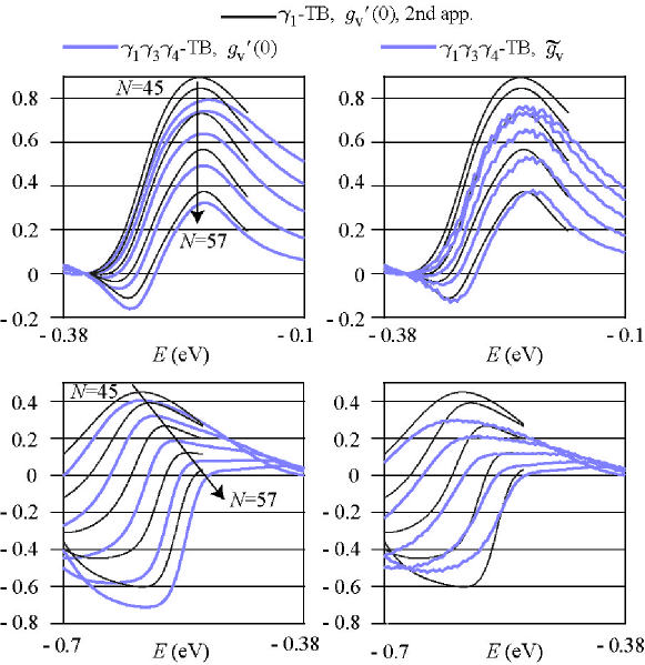
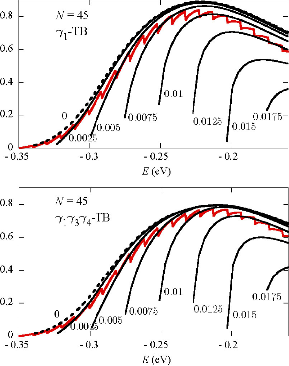
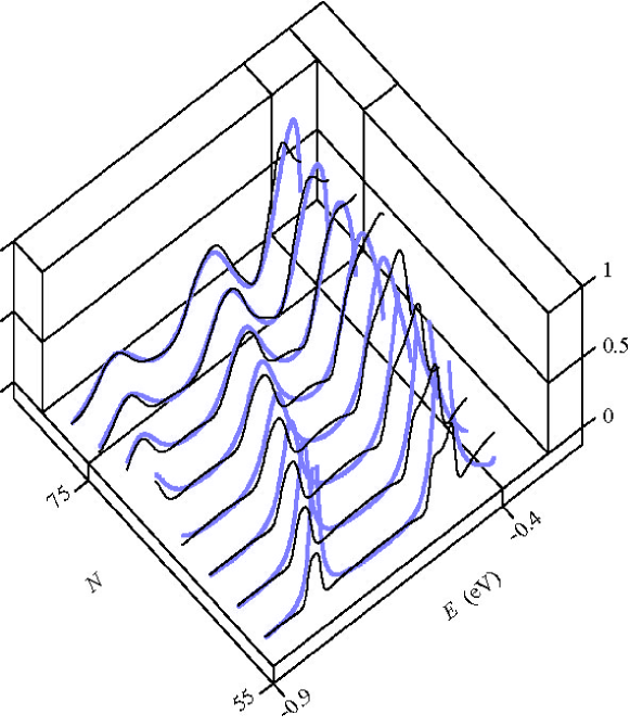
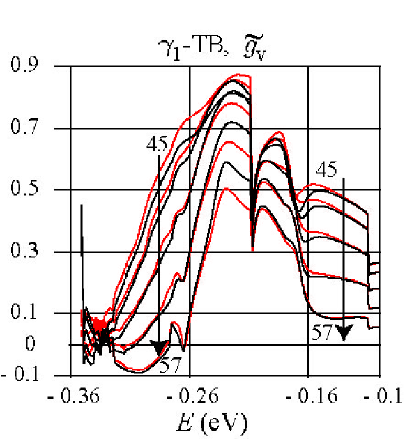
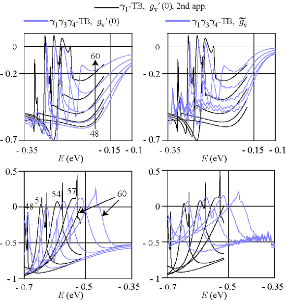
Figures 6 and 7 show the data on $\varepsilon=0.35$ eV and $\varepsilon=0$, respectively. $N$ increases from 45 to 57 (from 57 to 69) in Fig. 6 (Fig. 7), where $N$ is limited to a multiple of three. In Fig. 6, $E$ changes from $-0.38$ eV to $-0.1$ eV (from $-0.7$ eV to $-0.38$ eV ) in the top (bottom) panels. The $E$ ranges partially overlap the gap $|E|<0.166$ eV and pseudogap 0.35 eV $<|E|<0.514$ eV in Fig. 6. Figure 7 includes a part of the pseudogap $|E|<$ 0.377 eV. Blue lines represent the $\gamma_{1}\gamma_{3}\gamma_{4}$-TB data, indicating $g^{\prime}_{\rm v}(0)$ in the left panels and $\tilde{g}_{\rm v}$ in the right panels. The left panels are identical to the right panels in the black lines representing the second approximation of $g^{\prime}_{\rm v}(0)$. Each pair of identical black lines helps compare the left and right panels in the blue lines. In the gap and pseudogap, there are no black lines, but the blue lines confirm the suppression of $g^{\prime}_{\rm v}(0)$ and $\tilde{g}_{\rm v}$. The second approximation excellently reproduces the $T_{\nu,\nu^{\prime}}(0)$ of the exact $\gamma_{1}$-TB calculation, as Fig. 5 shows. Thus, $\gamma_{2}$ and $\gamma_{3}$ are the leading causes of the slight difference between the black and blue lines in the left panels and have only minor effects on $g^{\prime}_{\rm v}(0)$. On the other hand, $g^{\prime}_{\rm v}(\kappa)$ with nonzero $\kappa$ causes differences between the left and right panels in blue lines. Figure 8 displays the decomposition of $\tilde{g}_{\rm v}$ into $g^{\prime}_{\rm v}(\kappa)$ and elucidates the $\kappa$ effect for the highest $\tilde{g}_{\rm v}$ line of Fig. 6 (top panel, $N=45$). The top and bottom panels correspond to the $\gamma_{1}$-TB and $\gamma_{1}\gamma_{3}\gamma_{4}$-TB models, respectively. The solid black lines represent $g^{\prime}_{\rm v}(\kappa)$ for seven $\kappa^{\prime}$s, $\kappa/\pi=0.0025m$ ($m=1,2,\cdots,7)$. The black dashed lines represent the exact $g^{\prime}_{\rm v}(0)$ and are essentially the same as the second approximation of $g^{\prime}_{\rm v}(0)$. The eight black lines contribute to $\tilde{g}_{\rm v}$ when $N_{y}=400$ and $-0.35$ eV $<E<-0.16$ eV. As has been defined by Eqs. (6) and (10), $\tilde{g}_{\rm v}$ equals the sum of $g^{\prime}(\kappa)$ divided by $2M+1$, where the channel number $2M+1$ changes with $E$ according to Eq. (9). For example, $(E,2M+1)=(-0.34$ eV, 1) and $(-0.26$ eV, 7) when $N_{y}=400$. The red lines display $\tilde{g}_{\rm v}$ computed for the width $N_{y}=1000$, where the small notches reflect the finite $N_{y}$. As $N_{y}$ increases, the $\tilde{g}_{\rm v}$ line becomes smooth and independent of $N_{y}$. The monolayer energy gap $||E|-\varepsilon|<|\gamma_{0}\sin\kappa|$, which originates from Eq. (8), widens as $|\kappa|$ increases, and thus, only small $|\kappa|$’s contribute to the red lines in Fig. 8. In this small range of $\kappa$, $\tilde{g}_{\rm v}$ is close to $g^{\prime}_{\rm v}(0)$ as $g^{\prime}_{\rm v}(\kappa)$ is continuous with respect to $\kappa$. This is the reason why the blue lines of the left panels are similar to those of the right panels in Fig. 6. Figure 8 also proves that the $\gamma_{1}$-TB and $\gamma_{1}\gamma_{3}\gamma_{4}$-TB models produce essentially the same $\tilde{g}_{\rm v}$ except that $\gamma_{3}$ and $\gamma_{4}$ lower the peak slightly. In Ref. [105] , this smallness of $\gamma_{3},\gamma_{4}$ effects is discussed. These results indicate that the second approximation $g^{\prime}_{\rm v}(0)$ is very close to $\tilde{g}_{\rm v}$. In the case of $\varepsilon=0$, however, this is not true as discussed below.

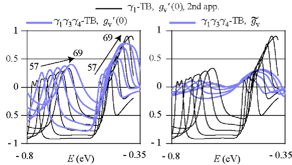
Figure 9 displays $g^{\prime}_{\rm v}(\kappa)$ of zero $\varepsilon$ for five $\kappa$’s, $\kappa/\pi=0,0.01,\cdots,0.04$ in case $\varepsilon=0$ and $N=69$, corresponding to the highest $\tilde{g}_{\rm v}$ peak in Fig. 7. The solid and dashed lines are calculated using the $\gamma_{1}$-TB and $\gamma_{1}\gamma_{3}\gamma_{4}$-TB models, respectively. Thick (thin) lines correspond to zero (nonzero) $\kappa$. In the pseudogap $|E|<\gamma_{1}$, $g^{\prime}_{\rm v}(\kappa)$ is suppressed. The peak height of $g^{\prime}_{\rm v}(0)$ is comparable to that in Fig. 8. Compared with Fig. 8, however, a wider range of $\kappa$ contributes to $\tilde{g}_{\rm v}$ in Fig. 7. When $\tilde{g}_{\rm v}$ reaches the maximum, the maximum effective $|\kappa|/\pi$ equals 0.013 in Fig. 6 and 0.045 in Fig. 7. As $\kappa$ increases, the $g^{\prime}_{\rm v}(\kappa)$ of Fig. 9 decreases to negative values and lowers the maximum $\tilde{g}_{\rm v}$ peak height shown in Fig. 7 compared with that shown in Fig. 6.

Figure 8: (Color online) $\tilde{g}_{\rm v}$ (red lines) and $g^{\prime}_{\rm v}(\kappa)$ (black lines) in the case of $\varepsilon=0.35$ eV, $N=45$, and $N_{y}=1000$, calculated using the $\gamma_{1}$-TB (top panel) and $\gamma_{1}\gamma_{3}\gamma_{4}$-TB models (bottom panel). The numerical values attached to each black line represent $\kappa/\pi$.

Figure 9: (Color online) $g^{\prime}_{\rm v}(\kappa)$ in the case of $\varepsilon=0$, and $N=69$. The numerical values attached to each line represent $\kappa/\pi$. The solid and dashed lines represent values calculated using the $\gamma_{1}$-TB and $\gamma_{1}\gamma_{3}\gamma_{4}$-TB models, respectively. Thick (thin) lines correspond to zero (nonzero) $\kappa$.

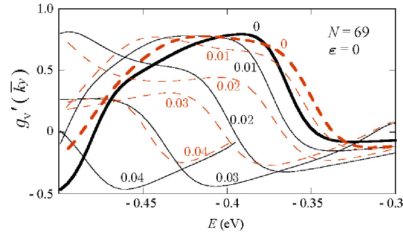
Arrows indicate the shift of the peaks with $N$ in Figs. 6 and 7. In the outer $E$, the peak energy $E$ approaches zero as $N$ increases. This shift comes from the phases $|\theta_{\pm}|N$ of Eq. (53), where $|\theta_{\pm}|$ increases with $|E|$ in the outer $E$. In the inner $E$, however, only the peak height changes with an almost constant peak energy (top panels in Fig. 6). This contrast suggests the difference between the outer and inner $E$ regions in the VCR origin. As shown in Figs. 1 and 4 , $I_{\xi}(\nu)\equiv|(\nu,1)\vec{d}^{\;\xi}_{\sigma,l}|^{2}/|\vec{d}^{\;\xi}_{\sigma,l}|^{2}=(1+\nu\alpha_{\xi})^{2}/(1+\alpha_{\xi}^{2})$ represents the monolayer $\xi$–bilayer matching, where $\xi=\downarrow,\uparrow$, $\alpha_{\downarrow}=\sigma l\alpha_{l}$, and $\alpha_{\uparrow}=\alpha_{\downarrow}(E-\varepsilon)/(E+\varepsilon)$. The product of monolayer–bilayer matchings $I_{\downarrow}(\pm)I_{\uparrow}(\mp)$ corresponds to the VCR and comes near the upper limit when (i) $\alpha_{\downarrow}\simeq-\alpha_{\uparrow}\simeq\pm 1$. Since $\alpha_{\uparrow}/\alpha_{\downarrow}=(E-\varepsilon)/(E+\varepsilon)$ , condition (i) requires $E\simeq 0$. The gap region $|E|<\Delta$ suppresses the transport near the zero energy, and thus the optimized $E$ comes at the gap edge $\pm\Delta$, followed by $\alpha_{\downarrow}=\sigma l(1\pm\sqrt{1+q})/\sqrt{2+q}$. When $q\gg 1$, this $\alpha_{\downarrow}$ satisfies condition (i). The condition $E\simeq\Delta$ is independent of $N$ and corresponds to the constant peak energy in the top panels of Fig. 6. For a large interlayer transmission rate, the wave function must be extended between the two layers, and thus the interlayer probability ratio $\tilde{\beta}_{l}\equiv|\vec{d}_{\sigma,l}^{\;\uparrow}|/\vec{d}_{\sigma,l}^{\;\downarrow}|$ must be close to one. We define the interlayer matching $I_{\downarrow\uparrow}\equiv 4/(\tilde{\beta}_{l}+\tilde{\beta}_{l}^{-1})^{2}$, since this $I_{\downarrow\uparrow}$ increases as $\tilde{\beta}_{l}$ approaches one. Interestingly, $I_{\downarrow\uparrow}$ is close to Eq. (50) when $|E|\simeq\Delta\ll\varepsilon$ and $\tilde{\beta}_{l}\simeq|\beta_{l}|$, suggesting the contributions of $\beta_{l}$ to the VCR. When $|E|\gg\Delta^{\prime}$, on the other hand, the monolayer–bilayer matching product $I_{\downarrow}(\pm)I_{\uparrow}(\mp)$ becomes inversely proportional to $E^{2}$, implying the physical origin of the factor $E^{-2}$ in Eq. (53).

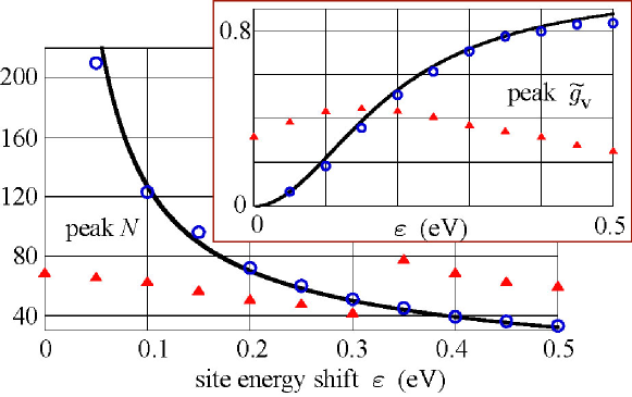
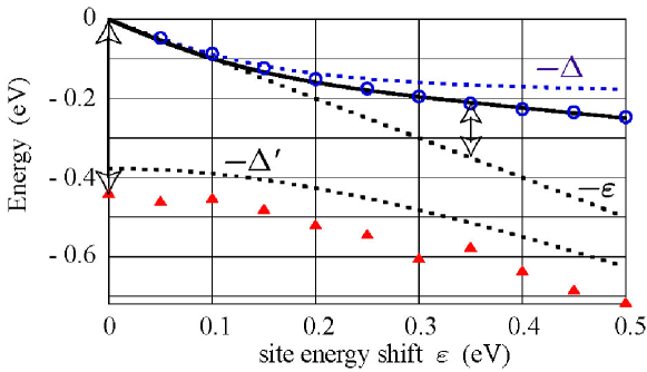
Circles (triangles) in Figs. 10 and 11 represent the highest $\tilde{g}_{\rm v}$ peak data in the inner (outer) $E$ region. These data are calculated using $\gamma_{1}\gamma_{3}\gamma_{4}$-TB model in the ranges $|E|<1.2$ eV and $N\leq 282$, for eleven $\varepsilon$’s, $\varepsilon=0.05m$ eV $(m=0,1,\cdots,10)$. Figure 10 shows the peak height and peak $N$. Figure 11 shows the peak $E$. Solid lines represent values obtained using Eqs. (50), (51), and (52), which accurately coincide with the circles. The dotted lines in Fig. 11 are the gap and pseudogap edge energies. Figures 10 and 11 include the inner $E$ peak $(E,N,\tilde{g}_{\rm v})=(-0.21$ eV, 45, 0.77) in Fig. 6 and the outer $E$ peak $(E,N,\tilde{g}_{\rm v})=(-0.44$ eV, 69, 0.32) in Fig. 7. Concerning the absolute and relative VCR, $(g_{\rm v},g_{\rm v}/g)=(0.042,0.47)$ for the former and (0.057, 0.24) for the latter. Notably, the former $g_{\rm v}/g$ reaches near the upper limit 0.5 corresponding to the perfect VCR ($T_{+,-}=T_{-,+}=1$). Compared with the zero $\varepsilon$ case, the absolute VCR slightly decreases, but the relative VCR significantly improves. The two vertical arrows in Fig. 11 represent $||E|-\varepsilon|$ at the above-mentioned two peaks, whereas Eq. (9) indicates the effective $\kappa$ range $|\kappa|<||E|-\varepsilon|/|\gamma_{0}$. These arrows illustrate that the subband effects are more significant in Fig. 7 than in Fig. 6. In the top panel of Fig. 10, the outer $E$ peak first increases with $\varepsilon$ but declines when $\varepsilon$ exceeds 0.15 eV. The initial climb comes from the shrinkage of the effective $\kappa$ range. As the peak $E$ becomes distant from zero, the factor $\gamma_{1}^{2}/E^{2}$ of Eq. (53) causes the later decline. In contrast, the inner $E$ peak continues to grow with $\varepsilon$ and rise above the outer peak. The perturbative formula in Ref. [66] is consistent with Eq. (53), but irrelevant to the inner $E$ peak [103].

Figure 10: (Color online) Height and $N$ of the highest $\tilde{g}_{\rm v}$ peak of the $\downarrow\uparrow$ junction calculated using the $\gamma_{1}\gamma_{3}\gamma_{4}$-TB model in the range $|E|<1.2$ eV and $N\leq 282$, for eleven $\varepsilon$’s, $\varepsilon=0.05m$ eV $(m=0,1,\cdots,10)$. Circles and triangles correspond to inner and outer $E$ regions, respectively. The transverse width $3N_{y}a_{\rm c}$ is 3000$a_{\rm c}$. The solid lines represent $\tilde{g}_{\rm v}=q/(1+q)$ and Eq. (51).

Figure 11: (Color online) Energies corresponding to the data in Fig. 10. The solid line represents values obtained using Eq. (52). The dotted lines show the gap and pseudogap edges. The vertical arrows represent $||E|-\varepsilon|$ for the triangle of $\varepsilon=0$ and the circle of $\varepsilon=$ 0.35 eV.

Equation (53) derives its validity from condition $|E|\gg\gamma_{1}\sqrt{1+q}$ in Appendix B, whereas Fig. 11 indicates that the outer $E$ peak appears near the pseudogap edge, $\pm\gamma_{1}\sqrt{1+\frac{q}{4}}$. This might weaken the effectiveness of Eq. (53) discussed above. Figure 12 dissolves this uncertainty, where the black and blue lines represent the VCR transmission rate $T_{\pm,\mp}$ of Eqs. (45) and (53), respectively, in the case of $\varepsilon=0$. Surprisingly, the blue lines coincide well with the black lines even when $|E|$ is close to $\gamma_{1}$. The blue lines overestimate the peak heights for $N$ between 57 and 63, but coincide well with the black lines for other $N$ values. The decay of $T_{\pm,\mp}$ with $|E|$ certainly appears in the black lines. Overall, Eq. (53) reproduces the peak position $(E,N)$ of Eq. (45). These results mean that the condition $|E|\gg\gamma_{1}\sqrt{1+q}$ is not necessary but sufficient for the effectiveness of Eq. (53). Although we have not obtained the necessary and sufficient condition yet, the $E^{-2}$ factor that comes from the monolayer–bilayer matching certainly causes the decline of the outer $E$ peak.

Figure 12: (Color online) VCR transmission rate $T_{\pm,\mp}$ in the case of $\varepsilon=0$. Black and blue lines represent values calculated using Eqs. (45) and (53), respectively. $N$ is limited to a multiple of three.

The $\tilde{g}_{\rm v}$ oscillates periodically as a function of $N$, and the considered $N$ range in Fig. 10 $(N\leq 282)$ is sufficient to include the global maximum of $\tilde{g}_{\rm v}$. The height of the $m$’th $g^{\prime}_{\rm v}(0)$ peak at $N\simeq m\pi/\theta_{0}$ in the inner $E$ is almost constant irrespective of $m$ in the second approximation, but gradually decreases with $m$ in the exact $\gamma_{1}$-TB calculation. This difference comes from the deviation of the average wave number $\frac{1}{2}(k^{(+)}_{l}+k^{(-)}_{l})$ from $\frac{4\pi}{3a}$. The second approximation neglects this deviation. In the exact $\gamma_{1}$-TB calculation, the deviation of the phase $(k^{(+)}_{l}+k^{(-)}_{l})Na/4$ from $\frac{2}{3}\pi N$ increases with $N$, followed by the decay of the peak height. $\gamma_{3}$ and $\gamma_{4}$ also induce the phase shift. Additionally, the peak period in $g^{\prime}_{\rm v}(\kappa)$ deviates from $\pi/\theta_{0}$ as $|\kappa|$ increases. These effects cause the decay of the $\tilde{g}_{\rm v}$ peak with $N$ in the inner $E$.

In the calculation presented so far, we assume the perfect armchair termination with no zigzag edge. To see the validity of this assumption, we replace the periodic condition with the open boundary condition at positions $\frac{y}{a_{\rm c}}=2.5,151.5$ (7.5, 156.5) of the $\uparrow$ layer ($\downarrow$ layer) in the $\downarrow\uparrow$ junction. This junction is equivalent to partially overlapped (50,50) zigzag graphene ribbons (ZGRs). We also consider addimers bonded with the armchair edges as in Fig. 2. The positions of the addimers vary randomly depending on the samples, and we consider six addimers at $(\frac{x}{a},\frac{y}{a_{\rm c}})=(0,32)$,(0,92),(0,122), $(N/2,46)$, $(N/2,67)$, and $(N/2,97)$ as a case of low coverage. Figure 13 corresponds to the top panels of Fig. 6, where red (black) lines indicate the exact $\gamma_{1}$-TB calculation of $\tilde{g}_{\rm v}$ of the ZGR junction with no addimer (with the six addimers). The $\tilde{g}_{\rm v}$ curve is almost the same as that in Fig. 6 and the nearly perfect VCR survives the imperfections. The sharp dips at $E=-0.21$ eV and $-0.11$ eV correspond to the subband edge energies. Additionally, a nearly flat band of zigzag edge increases $\tilde{g}_{\rm v}$ near the Dirac points of single layers, $|E|\simeq\varepsilon$. As the ZGR width increases, however, these effects weaken and the $\tilde{g}_{\rm v}$ curve in Fig. 6 recovers.

Figure 13: (Color online) Exact $\tilde{g}_{\rm v}$ of partially overlapped (50,50) zigzag graphene ribbons (ZGR) calculated using $\gamma_{1}$-TB in the case of $N=45,48,51,54,$ and 57, and $\varepsilon=0.35$ eV. Red and black lines correspond to the perfect armchair edges and the armchair edges with six addimers, respectively. See the main text and Fig. 2 for the addimers and ZGR.

4.2 $\downarrow\downarrow$ junction

As Eq. (9) shows, the effective $\kappa$ range $|\kappa|<|E+\varepsilon|/|\gamma_{0}|$ is wider for positive $E$ than for negative $E$. It follows that the $\tilde{g}_{\rm v}$ peaks in the negative $E$ region are higher than those in the positive $E$ region. In the case of the $\downarrow\uparrow$ junction, an integer, $N/3$, is a necessary condition for a near perfect $\tilde{g}_{\rm v}$ because the relation $T_{+,-}\simeq T_{-,+}$ holds under this condition. Contrarily, the mirror symmetry of the $\downarrow\downarrow$ junction guarantees the relation $T_{+,-}=T_{-,+}$, irrespective of $N$. Nevertheless, the $\tilde{g}_{\rm v}$ peak tends to be higher with an integer $N/3$ than a non-integer $N/3$. We speculate that constructive interference between the $\vec{f}_{A}$ and $\vec{f}_{B}$ modes in Eq. (55) increases $\tilde{g}_{\rm v}$. As our interest lies in high $\tilde{g}_{\rm v}$, we present data on the negative $E$ and $N$ being a multiple of three. Figures 14 and 15 represent the VCR data in the cases of $\varepsilon=0.35$ eV and $\varepsilon=0$, respectively. The black lines in Figs. 14 and 15 display the second approximation of $g^{\prime}_{\rm v}(0)$. The blue lines show the exact data of $g^{\prime}_{\rm v}(0)$ ($\tilde{g}_{\rm v}$) calculated using the $\gamma_{1}\gamma_{3}\gamma_{4}$-TB model in the left (right) panel. Overall, Figs. 14 and 15 have the same format as that in Figs. 6 and 7. The good agreement between the black and blue lines in the left panels indicates the effectiveness of the second approximation of $g^{\prime}_{\rm v}(0)$ and the insignificantly small effects of $\gamma_{3}$ and $\gamma_{4}$. The $(E,N)$ ranges in Figs. 14 and 15 include or lie around the highest $\tilde{g}_{\rm v}$ peaks searched in the ranges $|E|<1.2$ eV and $N\leq 282$; $(E,N,\tilde{g}_{\rm v})=(-0.47$ eV$,60,0.20)$ in the case of $\varepsilon=$ 0.35 eV and $(-0.51$ eV, $36,0.45)$ in the case of $\varepsilon=0$. In Fig. 15, the blue line peaks reach about 0.7 in the left panel but remain less than 0.45 in the right panel. This reduction in $\tilde{g}_{\rm v}$ comes from the $\kappa$ effect in the same way as Fig. 7. The monolayer–bilayer matching product of the $\downarrow\downarrow$ junction is defined as $I_{\downarrow}(\pm)I_{\downarrow}(\mp)$ in the same way as $I_{\downarrow}(\pm)I_{\uparrow}(\mp)$ of the $\downarrow\uparrow$ junction. This product $I_{\downarrow}(\pm)I_{\downarrow}(\mp)$ becomes also proportional to $E^{-2}$ and explains the similarity between Figs. 7 and 15. The outer $E$ peak comes near the pseudogap edge $|E|=\Delta^{\prime}$ and decreases its height with $\varepsilon$ in the same way as the outer $E$ peak of the $\downarrow\uparrow$ junction. When $\varepsilon=0$, the outer $E$ peak of the $\downarrow\downarrow$ junction is slightly higher than that of the $\downarrow\uparrow$ junction. When $\varepsilon$ exceeds 0.2 eV, however, the inner $E$ peak of the $\downarrow\uparrow$ junction is dominant over the $\downarrow\downarrow$ junction peak.

Figure 14: (Color online) VCR data of $\downarrow\downarrow$ junction in the case of $\varepsilon=0.35$ eV, $N_{y}=1000$, and $N=48,51,54,57,60$ with almost the same format as in Fig. 6.

Figure 15: (Color online) VCR data of $\downarrow\downarrow$ junction in the case of $\varepsilon=0$, $N_{y}=1000$, and $N=42,45,48,51,$ and 54 with almost the same format as Fig. 7.

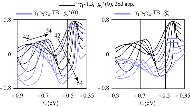
The second approximation is effective as shown in both Figs. 14 and 6, where the monolayer energy gap suppresses the $\kappa$ effect. In the inner $E$ region of $\varepsilon=$ 0.35 eV, $\tilde{g}_{\rm v}$ is typically negative and about 0.1 at the most. This reduction in $\tilde{g}_{\rm v}$ is reasonable. As $\varepsilon$ increases, interlayer resonance degrades, and the $\downarrow$ layer works as an isolate-perfect layer with no intervalley scattering. In the case of the $\downarrow\uparrow$ junction, however, the electron must flow between the $\downarrow$ and $\uparrow$ layers, and thus, the $\downarrow$ layer cannot be isolated by increasing $\varepsilon$. The fine notches from the finite $N_{y}$ effect are more visible in Fig. 14 than in Fig. 6. The $g^{\prime}(\kappa)$ of the $\downarrow\downarrow$ junction suddenly changes from a considerably negative value to zero when $|\kappa|$ exceeds $|E+\varepsilon|/|\gamma_{0}|$, because of the $\downarrow$ layer energy gap $|E+\varepsilon|<|\gamma_{0}\sin\kappa|$. This sudden change brings remarkable notches to Fig. 14. On the other hand, $g^{\prime}(\kappa)$ of the $\downarrow\uparrow$ junction with the energy $E\simeq-\varepsilon$ is close to zero, irrespective of $\kappa$. Thus the finite $N_{y}$ effect is inconspicuous in Fig. 6.

5 Detection in Experiments

The SG structure was experimentally observed in a Li-intercalated graphene[110]. However, the VCR occurs in the G–SG–G double junctions, not in the SG alone [62, 63, 64]. The G–SG boundary control remains undeveloped, whereas the established G layer alignment technique is advantageous to the po-G measurement [111].

Figure 16: Experimental detection of VCR via the bulk states. (a) Nonlocal resistance $R_{nl}=V/I$, where the current $I$ from contacts 1 to 2 induces the voltage between contacts 3 and 4. The central part is similar to the $\downarrow\uparrow$ junction. The thick lines represent the zigzag edges. (b) Optical detection with the second harmonic generation. Dashed circles represent the illuminated areas.

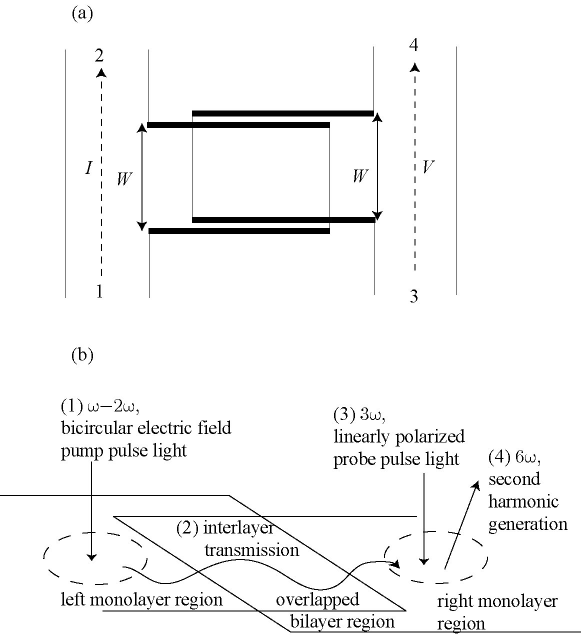
Figure 16(a) shows a scheme of an experiment that proves that the bulk states drive the VCR. The central part is similar to the $\downarrow\uparrow$ junction with a finite transverse width $W$. The thick lines represent the zigzag edges. As the width $W$ increases, the bulk contribution becomes dominant and reduces the difference between the open and periodic boundary conditions. The $R_{nl}$ equals $I/(V_{3}-V_{4})$, where $I$ is the charge current from 1 to 2 probes, and $V_{3}$ ($V_{4}$) is the electric potential at contact 3 (4). It is a VCR signature that the vertical gate voltage changes the $R_{nl}$ sign. The top and bottom gates control the parameters $E$ and $\varepsilon$. In contrast to the VCR of the zigzag edge states [61], the bulk states carry the VC. The edge is an imperfection of the infinite perfect crystal and cannot always be controlled. However, its effects become negligible as the width $W$ increases. Notably, reducing imperfections is an effective strategy for reproducible outcomes, especially in industrial use.

In electric measurement, the current terminals, $(V_{L},V_{R})$ in Fig. 1 and (1, 2) in Fig. 15, inevitably connect the sample edges and enhance the edge influence on the current. In contrast, we can exclude the current terminals in the optical measurements. The valley polarization can be generated by either circularly [49, 50, 51, 52, 53, 54, 55, 56] or linearly polarized light [57, 58]. We can also measure the valley polarization by optical second harmonic (SH) generation [59, 60]. Steps (1)–(4) in Fig. 16(b) illustrate an optical measurement method according to Ref. [55] . (1) The left monolayer region is illuminated with the pump pulse $\omega$ -$2\omega$ bicircular field, where $\omega$ denotes the principal angular frequency. This illumination induces the spatial gradient of valley concentration, followed by the valley-dependent diffusion of electrons, i.e., VC. (2) The induced VC is transmitted through the bilayer region with the sign reversed by the vertical gate. Consequently, the right monolayer has the opposite valley polarization compared with the left. (3) The linearly polarized probe light of the angular frequency $3\omega$ is incident to the right monolayer region and generates the SH. (4) The valley polarization in the right monolayer is detectable with the phase of the SH ($6\omega$ angular frequency). The illuminated areas in steps (1) and (3) are near the bilayer region but are restricted to each monolayer region. We can also measure the electron transit time in step (2) from the delay time of the probe pulse.

In the experiment described in Ref. [21] , the displacement field $D$ times the interlayer distance $a_{\downarrow\uparrow}$ reaches about 0.5 V with a band gap of 0.14 eV, where $D$ represents the microscopic electric field felt by the graphene electrons. These data are comparable to $(2\varepsilon,\Delta)=(0.7,0.166)$ eV for the high VCR $\tilde{g}_{\rm v}=0.8$, suggesting the technical feasibility of the present results. Since the carriers and surrounding materials have screening effects, more realistic self-consistent calculations are necessary for the relationship between $eDa_{\downarrow\uparrow}$ and $2\varepsilon$. Additionally, the high $D$ might modify the interlayer transfers $\gamma_{1}$, $\gamma_{3}$, and $\gamma_{4}$. The present analytic formulas contain no fitting parameter other than the Hamiltonian elements and thus can be adapted to these advanced calculations [102, 112].

6 Summary and Conclusion

We discuss the $\downarrow\xi$ junction $(\xi=\downarrow,\uparrow)$, which denotes the double junction in a series of the left layer $\downarrow$, AB stacking bilayer, and right layer $\xi$, where $\downarrow$ and $\uparrow$ are the extensions of the lower and upper layers from the bilayer, respectively. Using the $\gamma_{1}$-TB and $\gamma_{1}\gamma_{3}\gamma_{4}$-TB models, we calculate the transmission rate $T_{\nu^{\prime},\nu}$ from the left valley $K_{\nu}$ to the right valley $K_{\nu^{\prime}}$ as a function of the energy, the longitudinal bilayer length, and the lateral wave number $\kappa$. The VCR transmission rate $g^{\prime}_{\rm v}(\kappa)=\frac{1}{2}\sum_{\nu}\left[T_{-\nu,\nu}(\kappa)-T_{\nu,\nu}(\kappa)\right]$ averages out at $\tilde{g}_{\rm v}$ per $\kappa$. The present paper is the first report on the two VCR origins of the po-G: monolayer–bilayer matching and interlayer matching. These two origins refer to ‘wave function’ matching in position space (not in momentum space) and present an intuitive picture. Notably, the vertical electric field enhances the interlayer matching near the bilayer gap edge and provides the nearly ‘pure’ VCR. A pure VC changes into an almost pure VC with an inverse sign and a similar intensity. This enhancement occurs only when the electrons are forced to flow vertically, i.e., only in the $\downarrow\uparrow$ junction. On the other hand, monolayer–bilayer matching is adequate for the VCR in the $\downarrow\uparrow$ and $\downarrow\downarrow$ junctions but weakens under the vertical field.

Using the $\gamma_{1}$-TB model, we derive the analytical $T_{\nu^{\prime},\nu}(0)$ formulas. Since $\gamma_{3}$, $\gamma_{4}$, and nonzero $|\kappa|$ have only minor effects on $\tilde{g}_{\rm v}$ near the bilayer gap edge, this formula is effective in the $\tilde{g}_{\rm v}$ peak of the $\downarrow\uparrow$ junction. The bilayer length is represented by $(N-2)a/2$ with an integer $N$ and the lattice constant $a$. Compared with the non-integer $N/3$ case, the integer $N/3$ case shows larger $g^{\prime}_{\rm v}(0)$ and yields Eq. (45) that reflects the periodic sublattice localization of Eq. (56). The peak $N$ satisfies the condition $\left||k_{0}|\frac{a}{2}-\frac{2}{3}\pi\right|N\simeq\pi$, where $k_{0}$ is the bilayer wave number at the gap edge.

In addition to the valley filter and valley splitter, the VCR is an essential function in valleytronics but is still in its infancy. An important contribution is a proposal for the experimental detection of the VCR driven by the bulk states. It will open a new field in valleytronics.

Appendix A VC Formulas

The probability conservation and the time-reversal symmetry guarantee

$$T^{\rightarrow}_{\nu,\nu^{\prime}}(\kappa)=T^{\leftarrow}_{-\nu^{\prime},-\nu}(-\kappa),$$ (57)

$$R^{\leftarrow}_{\nu,\nu^{\prime}}(\kappa)=R^{\leftarrow}_{-\nu^{\prime},-\nu}(-\kappa),$$ (58)

$$R^{\rightarrow}_{\nu,\nu^{\prime}}(\kappa)=R^{\rightarrow}_{-\nu^{\prime},-\nu}(-\kappa),$$ (59)

where $R$ and $T$ denote the reflection and transmission rates, respectively [113]. The superscript $\leftarrow$ ($\rightarrow$) corresponds to the incidence from the right (left) monolayer G. The right (left) subscript indicates the valley index before (after) the scattering. Equation (57) is abbreviated to $T_{\nu,\nu^{\prime}}(\kappa)$ in the main text. With this notation, Eq. (10) is equivalent to

$$\tilde{g}_{\rm v}=\frac{1}{2M+1}\left[g^{\prime}_{\rm v}(0)+\sum_{m=1}^{M}g^{\prime\prime}_{\rm v}(m\Delta\kappa)\right],$$ (60)

where

$$g^{\prime\prime}_{\rm v}(\kappa)=\sum_{\nu,\nu^{\prime}}\frac{-\nu\nu^{\prime}}{2}\left[T_{\nu^{\prime},\nu}^{\leftarrow}(\kappa)+T^{\rightarrow}_{\nu,\nu^{\prime}}(\kappa)\right].$$ (61)

The inversion of the $\varepsilon$ sign is equivalent to the $\pi$ rotation around the $y$ axis for the $\downarrow\uparrow$ junction. Since $g^{\prime\prime}(\kappa)$ is invariant under this rotation, Eq. (12) is true for the $\downarrow\uparrow$ junction. In contrast, the $\downarrow\downarrow$ junction does not satisfy Eq. (12) because this rotation is not equivalent to the $\varepsilon$ sign change.

Using the $\kappa$ average notation

$$\tilde{\diamondsuit}=\frac{1}{2M+1}\sum_{m=-M}^{M}\diamondsuit(m\Delta\kappa),$$ (62)

we can derive

$$\tilde{T}^{\rightarrow}_{\nu,\nu^{\prime}}=\tilde{T}^{\leftarrow}_{-\nu^{\prime},-\nu},$$ (63)

$$\tilde{R}^{\leftarrow}_{\nu,\nu^{\prime}}=\tilde{R}^{\leftarrow}_{-\nu^{\prime},-\nu},$$ (64)

$$\tilde{R}^{\rightarrow}_{\nu,\nu^{\prime}}=\tilde{R}^{\rightarrow}_{-\nu^{\prime},-\nu},$$ (65)

from Eqs. (57), (58), and (59). The VCs in the left (L) and right (R) monolayer regions are represented by

$$J_{\rm v}^{\rm L}=\sum_{\nu,\nu^{\prime}}\left[\left(\delta_{\nu,\nu^{\prime}}-\tilde{R}_{\nu^{\prime},\nu}^{\rightarrow}\right)\nu^{\prime}J_{\nu}^{\rightarrow}-\tilde{T}_{\nu^{\prime},\nu}^{\leftarrow}\nu^{\prime}J_{\nu}^{\leftarrow}\right]$$ (66)

and

$$J_{\rm v}^{\rm R}=\sum_{\nu,\nu^{\prime}}\left[\left(\tilde{R}_{\nu^{\prime},\nu}^{\leftarrow}-\delta_{\nu,\nu^{\prime}}\right)\nu^{\prime}J_{\nu}^{\leftarrow}+\tilde{T}_{\nu^{\prime},\nu}^{\rightarrow}\nu^{\prime}J_{\nu}^{\rightarrow}\right]$$ (67)

accompanied by the charge current

$$J = \sum_{\nu,\nu^{\prime}}\left[\left(\delta_{\nu,\nu^{\prime}}-\tilde{R}_{\nu^{\prime},\nu}^{\rightarrow}\right)J_{\nu}^{\rightarrow}-\tilde{T}_{\nu^{\prime},\nu}^{\leftarrow}J_{\nu}^{\leftarrow}\right]$$ (68)

$$= \sum_{\nu,\nu^{\prime}}\left[\left(\tilde{R}_{\nu^{\prime},\nu}^{\leftarrow}-\delta_{\nu,\nu^{\prime}}\right)J_{\nu}^{\leftarrow}+\tilde{T}_{\nu^{\prime},\nu}^{\rightarrow}J_{\nu}^{\rightarrow}\right],$$ (69)

where $J_{\nu}^{\rightarrow}$ ($J_{\nu}^{\leftarrow}$ ) denotes the non-negative incidence flow from the $K_{\nu}$ valley of region L (R).

Typical VCR occurs under two incidence conditions (i) $J_{\nu}^{\rightarrow}=1,J_{-\nu}^{\rightarrow}=J_{+}^{\leftarrow}=J_{-}^{\leftarrow}=0$ and (ii) $J_{\nu}^{\rightarrow}=J_{\nu}^{\leftarrow}=1,J_{-\nu}^{\rightarrow}=J_{-\nu}^{\leftarrow}=0$. Under condition (i), $J_{\rm v}^{\rm R}=\tilde{T}_{+,\nu}^{\rightarrow}-\tilde{T}_{-,\nu}^{\rightarrow}$,

$$J_{\rm v}^{\rm L}=\nu(1-\tilde{R}_{\nu,\nu}^{\rightarrow}+\tilde{R}_{-\nu,\nu}^{\rightarrow}),$$ (70)

and $J=\tilde{T}_{+,\nu}^{\rightarrow}+\tilde{T}_{-\,\nu}^{\rightarrow}$. Under condition (ii),

$$J_{\rm v}^{\rm L}=\nu(\tilde{R}_{-,+}^{\rightarrow}+\tilde{R}_{+,-}^{\rightarrow}+\tilde{T}_{-,+}^{\rightarrow}+\tilde{T}_{+,-}^{\rightarrow}),$$ (71)

$$J_{\rm v}^{\rm R}=-\nu(\tilde{R}_{-,+}^{\leftarrow}+\tilde{R}_{+,-}^{\leftarrow}+\tilde{T}_{-,+}^{\rightarrow}+\tilde{T}_{+,-}^{\rightarrow}),$$ (72)

and $J=\tilde{T}_{\nu,\nu}^{\rightarrow}-\tilde{T}_{-\nu,-\nu}^{\rightarrow}$. When $\tilde{g}_{\rm v}\simeq 1$, the reflection rates $R_{\nu,\nu^{\prime}}$ and intravalley transmission rates $T_{\pm,\pm}$ are near zero followed by the VCR $J_{\rm v}^{\rm L}\simeq-J_{\rm v}^{\rm R}$. In particular, the VCR of condition (ii) corresponds to the reversal of pure VC as $|J_{\rm v}|\simeq 2\gg|J|$. In the calculation with condition (ii) above, we use Eqs. (63), (64), and (65), and the probability conservation

$$\sum_{\nu^{\prime}}\tilde{T}_{\nu^{\prime},\nu}^{\leftarrow}+\tilde{R}_{\nu^{\prime},\nu}^{\leftarrow}=\sum_{\nu^{\prime}}\tilde{T}_{\nu^{\prime},\nu}^{\rightarrow}+\tilde{R}_{\nu^{\prime},\nu}^{\rightarrow}=1.$$ (73)

Appendix B Explicit Expressions of the Second Approximation

Except for the last paragraph, in the present Appendix, we discuss the $\downarrow\uparrow$ junction. In the case of the $\downarrow\uparrow$ junction,

$$G_{\;{}^{B}_{A}}=\frac{\gamma_{1}(|\theta_{\mp}|s_{-}-|\theta_{\pm}|s_{+})}{\sqrt{3}|\gamma_{0}|(\theta_{+}^{2}-\theta_{-}^{2})},$$ (74)

$${\rm Re}[F_{A}]=\frac{3\gamma_{0}^{2}|\theta_{+}\theta_{-}|}{\varepsilon^{2}-E^{2}}(Z+c_{+}c_{-})+s_{+}s_{-},$$ (75)

$${\rm Re}[F_{B}]=-Z-c_{+}c_{-}+\frac{3\gamma_{0}^{2}|\theta_{+}\theta_{-}|}{E^{2}-\varepsilon^{2}}s_{+}s_{-},$$ (76)

$${\rm Im}[F_{\;{}_{A}^{B}}] =\frac{\sqrt{3}|E\gamma_{0}|}{E^{2}-\varepsilon^{2}} \left[|\theta_{\pm}|s_{+}c_{-}+|\theta_{\mp}|s_{-}c_{+}\right.$$ (77)

$$\left.\mp\frac{4\varepsilon^{2}(|\theta_{\pm}|s_{+}c_{-}-|\theta_{\mp}|s_{-}c_{+})}{3\gamma_{0}^{2}(\theta_{+}^{2}-\theta_{-}^{2})}\right],$$

where

$$Z =\frac{2\gamma_{1}^{2}(E^{2}-\varepsilon^{2})}{9\gamma_{0}^{4}(\theta_{+}^{2}-\theta_{-}^{2})^{2}} \left[\left(1-\frac{\theta_{+}^{2}+\theta_{-}^{2}}{2|\theta_{+}\theta_{-}|}\right)s_{+}s_{-}\right.$$ (78)

$$\left.+2\sin^{2}\left(\frac{|\theta_{+}|-|\theta_{-}|}{2}N\right)\right],$$

$$c_{\pm}=\cos(\theta_{\pm}N),\;\;s_{\pm}=\sin(|\theta_{\pm}|N).$$ (79)

When $|E|$ approaches $\Delta$, $|\theta_{\pm}|$ converges to $\theta_{0}$, followed by the limits

$$\lim_{|\theta_{\pm}|\rightarrow\theta_{0}}G_{\;{}_{A}^{B}}=-\sqrt{\frac{1+q}{q(2+q)}}\;(\phi_{0}\cos\phi_{0}\pm\sin\phi_{0}),$$ (80)

$$\lim_{|\theta_{\pm}|\rightarrow\theta_{0}}F_{B} = -1-\frac{2}{q}+\frac{1+q}{(2+q)^{2}}(\phi_{0}^{2}-\sin^{2}\phi_{0})$$ (81)

$$+\frac{2}{q}\cos^{2}\phi_{0}-i\frac{\sin(2\phi_{0})}{q\sqrt{2+q}}+2i\frac{1+q}{q\sqrt{2+q}}\phi_{0},$$

and

$$\lim_{|\theta_{\pm}|\rightarrow\theta_{0}}F_{A} = 1+\frac{1+q}{q(2+q)}(\sin^{2}\phi_{0}-\phi_{0}^{2})$$ (82)

$$+\frac{2}{q}\cos^{2}\phi_{0}-i\frac{\sin(2\phi_{0})}{q\sqrt{2+q}}-2i\frac{1+q}{q\sqrt{2+q}}\phi_{0},$$

where $\phi_{0}=\theta_{0}N$. Under condition (49), the last terms become dominant in Eqs. (81) and (82). Equation (48) originates from these terms and Eq. (80).

Figure 17: (Color online) $|F|/2$ and $G$ calculated using Eqs. (74) (75), (76), and (77) in the case of $\varepsilon=0.35$ eV and $N=45$.

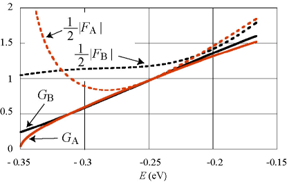
Figure 3 demonstrates that $|\theta_{+}|+|\theta_{-}|\simeq 2\theta_{0}$ when $|E|$ is near $\Delta$. This leads to the approximation

$$N|\theta_{\pm}|\simeq\pi(1\pm\varphi),$$ (83)

where $N\simeq\pi/\theta_{0}$ (Eq. (51)). When $|\varphi|<\frac{1}{3}$,

$$\Delta<|E|<\frac{\Delta}{3}\sqrt{11+q},$$ (84)

as is confirmed below. The smallness of $|\sin(\theta_{0}N)|$ is necessary for the derivation of the following approximate formulas from Eq. (83). Since $N/3$ is an integer, $\theta_{0}N$ equals $3\theta_{0}$ times an integer, and thus the minimum $|\sin(\theta_{0}N)|$ can reach $\sin(3\theta_{0}/2)$. The condition $q<8$ is equivalent to the condition $\sin(3\theta_{0}/2)<0.16$. First, we discuss the case $1<q<8$. The other case, $q<1$, is discussed later.

When $|E|$ reaches Eq. (52), Eq. (46) produces

$$\theta_{+}^{2}+\theta_{-}^{2}=\frac{10q(2+q)\gamma_{1}^{2}}{54(1+q)\gamma_{0}^{2}}.$$ (85)

This approximates

$$\theta_{+}^{2}+\theta_{-}^{2}\simeq\left[10-\frac{1}{(1+q)^{2}}\right]\frac{q(2+q)\gamma_{1}^{2}}{54(1+q)\gamma_{0}^{2}}$$ (86)

because $\frac{1}{(1+q)^{2}}\ll 10$. On the other hand, Eq. (46) guarantees an identity

$$\theta_{+}^{2}+\theta_{-}^{2}=\frac{3(\theta_{+}^{2}-\theta_{-}^{2})^{2}\gamma_{0}^{2}}{2(1+q)\gamma_{1}^{2}}+\frac{q(2+q)\gamma_{1}^{2}}{6(1+q)\gamma_{0}^{2}}.$$ (87)

Equations (86) and (87) result in

$$\theta_{+}^{2}-\theta_{-}^{2}\simeq\frac{q(2+q)\gamma_{1}^{2}}{9(1+q)\gamma_{0}^{2}}.$$ (88)

Equations (85) and (88) satisfy condition $|\theta_{+}|\simeq 2|\theta_{-}|$. When this condition and Eq. (83) hold, $\varphi\simeq\frac{1}{3}$. When Eq. (83) is effective, Eqs. (74), (75), (76), and (77) are approximated by

$$G_{B} \simeq G_{A}$$ (89)

$$\simeq \frac{\sin(\pi\varphi)}{\varphi}\sqrt{\frac{1+q}{q(2+q)}},$$ (90)

$${\rm Re}[F_{A}] \simeq \cos(2\pi\varphi)-\frac{1+q}{q(2+q)}\frac{\sin^{2}(\pi\varphi)}{\varphi^{2}}$$ (91)

$$+\frac{2}{q}\cos^{2}(\pi\varphi),$$

$${\rm Re}[F_{B}] \simeq -{\rm Re}[F_{A}]-\frac{2(1+q)\sin^{2}(\pi\varphi)}{q(2+q)^{2}\varphi^{2}}$$ (92)

$$+\frac{2}{q},$$

and

$${\rm Im}[F_{B}] \simeq -{\rm Im}[F_{A}]$$ (93)

$$\simeq \frac{1+q}{q}\sqrt{\varphi^{2}+\frac{1}{2+q}}\frac{\sin(2\pi\varphi)}{\varphi}.$$ (94)

Equations (92) and (93) suggest that $F_{\rm B}\simeq-F_{\rm A}$. Equations (75), (76), and (77) certainly satisfy the inequality $\left|{\rm Re}[F_{A}+F_{B}]/{\rm Im}[F]\right|<0.33$ when $1<q<8$ and $|\varphi|<\frac{1}{3}$. The relation $F_{\rm B}\simeq-F_{\rm A}$ and Eq. (89) cause the constructive VCR interference between the $\vec{f}_{A}$ and $\vec{f}_{B}$ modes as $g^{\prime}_{\rm v}(0)\simeq 4|G_{A}/F_{A}|^{2}$. Figure 17 displays $|F|/2$ and $G$ in the case of $\varepsilon=0.35$ eV $(q=3.45)$ and $N=45$ for the negative inner $E$ region $(-\varepsilon<E<-\Delta$), where $\pi/\theta_{0}=43.8$, $\Delta=0.166$ eV, and $\frac{\Delta}{3}\sqrt{11+q}=$ 0.21 eV. When $\varphi$ increases from 0 to $1/3$, $|F|/2$ approaches $G$, and the increase in $4G^{2}/|F|^{2}$ follows. On the other hand, Eqs. (74) and (75) prove that $|G_{A}/F_{A}|$ converges to zero at $|E|=|\varepsilon|$, followed by the disappearance of $g_{\rm v}^{\prime}(0)$. These results indicate that Eqs. (51) and (52) correspond to the $g^{\prime}_{\rm v}(0)$ peak. At the same time, Fig. B-1 shows that the variation of $|G/F|$ is minimal in the $E$ range (84). We have discussed above the case where $1<q<8$. As $q$ decreases from 1, on the other hand, the inner $E$ region shrinks, and thus the variation of $|G/F|$ in the inner $E$ region becomes small. In summary, the peak $g^{\prime}_{\rm v}(0)$ in conditions (51) and (52) is similar to $q/(1+q)$ calculated using Eqs. (48) and (51). When $|E|\gg\sqrt{4\varepsilon^{2}+\gamma_{1}^{2}}$, on the other hand, we derive Eq. (53) using $3\gamma_{0}^{2}\theta_{\pm}^{2}\simeq E^{2}\pm|E|\sqrt{4\varepsilon^{2}+\gamma_{1}^{2}}$, $Z\simeq\frac{1}{1+q}\sin^{2}\left(\frac{|\theta_{+}|-|\theta_{-}|}{2}N\right)$, ${\rm Im}(F_{A})\simeq{\rm Im}(F_{B})\simeq\sin\left((|\theta_{+}|+|\theta_{-}|)N\right)$, and $3\gamma_{0}^{2}|\theta_{+}\theta_{-}|/(E^{2}-\varepsilon^{2})\simeq 1$.

In the case of the $\downarrow\downarrow$ junction,

$${\rm Im}[F_{\;{}_{A}^{B}}] =\frac{\sqrt{3}|\gamma_{0}|}{(E+\varepsilon)} \left[|\theta_{\pm}|s_{+}c_{-}+|\theta_{\mp}|s_{-}c_{+}\right.$$ (95)

$$\left.+\frac{4\varepsilon E(|\theta_{\mp}|s_{-}c_{+}-|\theta_{\pm}|s_{+}c_{-})}{3\gamma_{0}^{2}(\theta_{+}^{2}-\theta_{-}^{2})}\right],$$

$$G_{\;{}_{A}^{B}} =\frac{\sqrt{3}|\gamma_{0}|}{2(E+\varepsilon)} \left[\frac{4\varepsilon E(|\theta_{\mp}|s_{-}-|\theta_{\pm}|s_{+})}{3\gamma_{0}^{2}(\theta_{+}^{2}-\theta_{-}^{2})}\right.$$ (96)

$$\left.+|\theta_{\mp}|s_{-}+|\theta_{\pm}|s_{+}\right],$$

$${\rm Re}[F_{B}]=Z+\left[\frac{3\gamma_{0}^{2}|\theta_{+}\theta_{-}|}{(E+\varepsilon)^{2}}+\frac{(E-\varepsilon)^{2}}{3\gamma_{0}^{2}|\theta_{+}\theta_{-}|}\right]s_{+}s_{-},$$ (97)

and

$${\rm Re}[F_{A}]=\frac{3\gamma_{0}^{2}|\theta_{+}\theta_{-}|}{(E+\varepsilon)^{2}}Z+2s_{+}s_{-}.$$ (98)

References

- [1] K. S. Novoselov, A. K. Geim, S. V. Morozov, D. Jiang, Y. Zhang, S. V. Dubonos, I. V. Grigorieva, and A. A. Firsov, Science 306, 666 (2004).
- [2] K. S. Novoselov, A. K. Geim, S. V. Morozov, D. Jiang, M. I. Katsnelson, I. V. Grigorieva, S. V. Dubonos, and A. A. Firsov, Nature 438, 197 (2005).
- [3] Y. Zhang, Y.-W. Tan, H. L. Stormer, and P. Kim, Nature 438, 201 (2005).
- [4] N. M. R. Peres, Rev. Mod. Phys. 82, 2673 (2010).
- [5] S. Das Sarma, S. Adam, E. H. Hwang, and E. Rossi, Rev. Mod. Phys. 83, 407 (2011).
- [6] A. H. Castro Neto, F. Guinea, N. M. R. Peres, K. S. Novoselov, and A. K. Geim, Rev. Mod. Phys. 81, 109 (2009).
- [7] J. Sinova, S. O. Valenzuela, J. Wunderlich, C. H. Back, and T. Jungwirth, Rev. Mod. Phys. 87, 1213 (2015).
- [8] D. Xiao, W. Yao, and Q. Niu, Phys. Rev. Lett. 99, 236809 (2007).
- [9] D. A. Abanin, S. V. Morozov, L. A. Ponomarenko, R. V. Gorbachev, A. S. Mayorov, M. I. Katsnelson, K. Watanabe, T. Taniguchi, K. S. Novoselov, L. S. Levitov, and A. K. Geim, Science 332, 328 (2011).
- [10] J. Balakrishnan, G. K. W. Koon, M. Jaiswal, A. H. Castro Neto, and B. Özyilmaz, Nat. Phys. 9, 284 (2013).
- [11] T. Völkl, D. Kochan, T. Ebnet, S. Ringer, D. Schiermeier, P. Nagler, T. Korn, C. Schüller, J. Fabian, D. Weiss, and J. Eroms, Phys. Rev. B 99, 085401 (2019).
- [12] M. Koshino and T. Ando, Phys. Rev. B 81, 195431 (2010).
- [13] S. A. Vitale, D. Nezich, J. O. Varghese, P. Kim, N. Gedik, P. Jarillo-Herrero, D. Xiao, and M. Rothschild, Small 14, 1801483 (2018).
- [14] M. Yamamoto, Y. Shimazaki, I. V. Borzenets, and S. Tarucha, J. Phys. Soc. Jpn 84, 121006 (2015).
- [15] M. B. Lundeberg and J. A. Folk, Science 346, 422 (2014).
- [16] A. Avsar, H. Ochoa, F. Guinea, B. Özyilmaz, B. J. van Wees, and I. J. Vera-Marun, Rev. Mod. Phys. 92, 021003 (2020).
- [17] I. Žutić, J. Fabian, and S. Das Sarma, Rev. Mod. Phys. 76, 323 (2004).
- [18] Y. Shimazaki, M. Yamamoto, I. V. Borzenets, K. Watanabe, T. Taniguchi, and S. Tarucha, Nature Phys. 11, 1032 (2015).
- [19] M. Sui, G. Chen, L. Ma, W.-Y. Shan, D. Tian, K. Watanabe, T. Taniguchi, X. Jin, W. Yao, D. Xiao, and Y. Zhang, Nature Phys. 11, 1027 (2015).
- [20] K. Endo, K. Komatsu, T. Iwasaki, E. Watanabe, D. Tsuya, K. Watanabe, T. Taniguchi, Y. Noguchi, Y. Wakayama, Y. Morita, and S. Moriyama, Appl. Phys. Lett. 114, 243105 (2019).
- [21] J. Yin, C. Tan, D. Barcons-Ruiz, I. Torre, K. Watanabe, T. Taniguchi, J. C. W. Song, J. Hone, and F. H. L. Koppens, Science 375, 1398 (2022).
- [22] Y. Jiang, T. Low, K. Chang, M. I. Katsnelson, and F. Guinea, Phys. Rev. Lett. 110, 046601 (2013).
- [23] R. V. Gorbachev, J. C. W. Song, G. L. Yu, A. V. Kretinin, F. Withers, Y. Cao, A. Mishchenko, I. V. Grigorieva, K. S. Novoselov, L. S. Levitov, and A. K. Geim, Science 346, 448 (2014).
- [24] K. Komatsu, Y. Morita, E. Watanabe, D. Tsuya, K. Watanabe, T. Taniguchi, and S. Moriyama, Sci. Adv. 4, eaaq0194 (2018).
- [25] J. H. J. Martiny, K. Kaasbjerg, and A.-P. Jauho, Phys. Rev. B 100, 155414 (2019).
- [26] J. Wang, Z. Lin, and K. S. Chan, Appl. Phys. Express 7, 125102 (2014).
- [27] Y. Liu, J. Song, Y. Li, Y. Liu, and Q. F. Sun, Phys. Rev. B 87, 195445 (2013).
- [28] J.-H. Chen, G. Autes, N. Alem, F. Gargiulo, A. Gautam, M. Linck, C. Kisielowski, O. V. Yazyev, S. G. Louie, and A. Zettl, Phys. Rev. B 89, 121407(R) (2014).
- [29] D. Gunlycke and C. T. White, Phys. Rev. Lett. 106, 136806 (2011).
- [30] V. H. Nguyen, S. Dechamps, P. Dollfus, and J.-C. Charlier, Phys. Rev. Lett. 117, 247702 (2016).
- [31] M. Settnes, S. R. Power, M. Brandbyge, and A.-P. Jauho, Phys. Rev. Lett. 117, 276801 (2016).
- [32] A. Chaves, L. Covaci, K. Y. Rakhimov, G. A. Farias, and F. M. Peeters, Phys. Rev. B 82, 205430 (2010).
- [33] L. S. Cavalcante, A. Chaves, D. R. da Costa, G. A. Farias, and F. M. Peeters, Phys. Rev. B 94, 075432 (2016).
- [34] T. Fujita, M. B. A. Jalil, and S. G. Tan, Appl. Phys. Lett. 97, 043508 (2010).
- [35] F. Zhai, X. Zhao, K. Chang, and H. Q. Xu, Phys. Rev. B, 82, 115442 (2010).
- [36] A. Rycerz, J. Tworzydlo, and C. W. J. Beenakker, Nat. Phys. 3, 172 (2007).
- [37] J. Nakabayashi, D. Yamamoto, and S. Kurihara, Phys. Rev. Lett. 102, 066803 (2009).
- [38] H. Santos, L. Chico, and L. Brey, Phys. Rev. Lett. 103, 086801 (2009).
- [39] M. Fujita, K. Wakabayashi, K. Nakada, and K. Kusakabe, J. Phys. Soc. Jpn. 65, 1920 (1996).
- [40] X. Z. Ying, M. X. Ye, and L. Balents, Phys. Rev. B 103, 115436 (2021).
- [41] C.-C. Hsu, M. L. Teague, J.-Q. Wang, and N.-C. Yeh, Sci. Adv. 6, eaat9488 (2020).
- [42] W. Ortiz, N. Szpak, and T. Stegmann, Phys. Rev. B 106, 035416 (2022).
- [43] F. Zhai and K. Chang, Phys. Rev. B 85, 155415 (2012).
- [44] J. L. Garcia-Pomar, A. Cortijo, and M. Nieto-Vesperinas, Phys. Rev. Lett. 100, 236801 (2008).
- [45] H. Schomerus, Phys. Rev. B 82, 165409 (2010).
- [46] A. R. Akhmerov, and C. W. J. Beenakker, Phys. Rev. Lett. 98, 157003 (2007).
- [47] K. Luo, T. Zhou, and W. Chen, Phys. Rev. B. 96, 245414 (2017).
- [48] S. Y. Li, Y. Su, Y. N. Ren, and L. He, Phys. Rev. Lett. 124, 106802 (2020).
- [49] K. Nakagahara and K. Wakabayashi, Phys. Rev. B 106, 075403 (2022).
- [50] W. Yao, D. Xiao, and Q. Niu, Phys. Rev. B 77, 235406 (2008).
- [51] R. Zhou, T. Guo, L. Huang, and K. Ullah, Mater. Today Phys. 23, 100649 (2022).
- [52] L.-L. Chang, Q.-P. Wu, Y.-Z. Li, R.-L. Zhang, M.-R. Liu, W.-Y. Li, F.-F. Liu, X.-B. Xiao, and Z.-F. Liu, Physica E 130, 114681 (2021).
- [53] S. A. O. Motlagh, F. Nematollahi, V. Apalkov, and M. I. Stockman, Phys. Rev. B 100, 115431 (2019).
- [54] N. Yoshikawa T. Tamaya, and K. Tanaka, Science 356, 736 (2017).
- [55] M. S. Mrudul, Á. Jiménez-Galán, M. Ivanov, and G. Dixit, Optica 8, 422 (2021).
- [56] M. S. Mrudul and G. Dixit, J. Phys. B 54, 224001 (2021).
- [57] H. K. Kelardeh, U. Saalmann, and J. M. Rost, Phys. Rev. Research, 4, L022014 (2022).
- [58] L. E. Golub, S. A. Tarasenko, M. V. Entin, and L. I. Magarill, Phys. Rev. B 84, 195408 (2011).
- [59] T. O. Wehling, A. Huber, A. I. Lichtenstein, and M. I. Katsnelson, Phys. Rev. B 91, 041404(R) (2015).
- [60] L. E. Golub, and S. A. Tarasenko, Phys. Rev. B 90, 201402(R) (2014).
- [61] A. R. Akhmerov, J. H. Bardarson, A. Rycerz, and C. W. J. Beenakker, Phys. Rev. B 77, 205416 (2008).
- [62] S. K. Wang and J. Wang, Phys. Rev. B 92, 075419 (2015).
- [63] J. J. Wang, S. Liu, J. Wang, and J.-F. Liu, Phys. Rev. B 98, 195436 (2018).
- [64] C. W. J. Beenakker, N. V. Gnezdilov, E. Dresselhaus, V. P. Ostroukh, Y. Herasymenko, I. Adagideli, and J. Tworzydlo, Phys. Rev. B 97, 241403(R) (2018).
- [65] R. Li, Z. Lin, and K. S. Chan, Physica E 113, 109 (2019).
- [66] R. Tamura, J. Phys. Soc. Jpn. 90, 114701 (2021); 92, 038001 (2023).
- [67] E. Cannavò, D. Marian, E. G. Marín, G. Iannaccone, and G. Fiori, Phys. Rev. B 104, 085433 (2021).
- [68] H. Z. Olyaei, P. Ribeiro, and E. V. Castro, Phys. Rev. B. 99, 205436 (2019).
- [69] C. J. Páez, A. L. C. Pereira, J. N. B. Rodrigues, and N. M. R. Peres, Phys. Rev. B. 92, 045426 (2015).
- [70] D. Yin, W. Liu, X. Li, L. Geng, X. Wang, and P. Huai, Appl. Phys. Lett. 103, 173519 (2013).
- [71] D. Valencia, J.-Q. Lu, J. Wu, F. Liu, F. Zhai, and Y.-J. Jiang, AIP Adv. 3, 102125 (2013).
- [72] J. Zheng, P. Guo, Z. Ren, Z. Jiang, J. Bai, and Z. Zhang, Appl. Phys. Lett. 101, 083101 (2012).
- [73] K. M. M. Habib, F. Zahid, and R. K. Lake, Appl. Phys. Lett. 98, 192112 (2011).
- [74] J. W. González, H. Santos, E. Prada, L. Brey, and L. Chico, Phys. Rev. B. 83, 205402 (2011).
- [75] X.-G. Li, I.-H. Chu, X. G. Zhang, and H.-P. Cheng, Phys. Rev. B 91, 195442 (2015).
- [76] J. W. González, H. Santos, M. Pacheco, L. Chico, and L. Brey, Phys. Rev. B 81, 195406 (2010).
- [77] H. Li, H. Li, Y. Zheng, and J. Niu, Physica B 406, 1385 (2011).
- [78] T. Nakanishi, M. Koshino, and T. Ando, Phys. Rev. B 82, 125428 (2010).
- [79] D. Xiao, M.-C. Chang, and Q. Niu, Rev. Mod. Phys. 82, 1959 (2010).
- [80] S. Roche, S. R. Power, B. K. Nikolić, J. H. García, and A. P. Jauho, J. Phys. Mater. 5, 021001 (2022).
- [81] T. Aktor, J. H. García, S. Roche, A.-P. Jauho, and S. R. Power, Phys. Rev. B 103, 115406 (2021).
- [82] F. Solomon and S. R. Power, Phys. Rev. B 103, 235435 (2021).
- [83] M. Azari and G. Kirczenow, Phys. Rev. B 95, 195424 (2017).
- [84] G. Kirczenow, Phys. Rev. B 92, 125425 (2015).
- [85] Z. Wang, H. Liu, H. Jiang, and X. C. Xie, Phys. Rev. B 100, 155423 (2019).
- [86] D. A. Abanin, A. V. Shytov, L. S. Levitov, and B. I. Halperin, Phys. Rev. B 79, 035304 (2009).
- [87] Y. D. Lensky, J. C. W. Song, P. Samutpraphoot, and L. S. Levitov, Phys. Rev. Lett. 114, 256601 (2015).
- [88] I. Martin, Y. M. Blanter, and A. F. Morpurgo, Phys. Rev. Lett. 100, 036804 (2008).
- [89] W. Yao, S. A. Yang, and Q. Niu, Phys. Rev. Lett. 102, 096801 (2009).
- [90] J. M. Marmolejo-Tejada, J. H. Garcia, M. D. Petrović, P.-H. Chang, X.-L. Sheng, A. Cresti, P. Plecháč, S. Roche, and B. K. Nikolić, J. Phys. Mater. 1, 015006 (2018).
- [91] M. J. H. Ku, T. X. Zhou, Q. Li, Y. J. Shin, J. K. Shi, C. Burch, L. E. Anderson, A. T. Pierce, Y. Xie, A. Hamo, U. Vool, H. Zhang, F. Casola, T. Taniguchi, K. Watanabe, M. M. Fogler, P. Kim, A. Yacoby, and R. L. Walsworth, Nature 583, 537 (2020).
- [92] D. A. Bandurin, I. Torre, R. K. Kumar, M. B. Shalom, A. Tomadin, A. Principi, G. H. Auton, E. Khestanova, K. S. Novoselov, I. V. Grigorieva, L. A. Ponomarenko, A. K. Geim, and M. Polini, Science 351, 1055 (2016).
- [93] H.-Y. Xie and A. Levchenko, Phys. Rev. B 99, 045434 (2019).
- [94] S. Danz, M. Titov, and B. N. Narozhny, Phys. Rev. B 102, 081114(R) (2020).
- [95] A. Aharon-Steinberg, A. Marguerite, D. J. Perello, K. Bagani, T. Holder, Y. Myasoedov, L. S. Levitov, A. K. Geim, and E. Zeldov, Nature 593, 528 (2021).
- [96] K. Gopinadhan, Y. J. Shin, R. Jalil, T. Venkatesan, A. K. Geim, A. H. Castro Neto, and H. Yang, Nat. Commun. 6, 8337 (2015).
- [97] J. Renard, M. Studer, and J. A. Folk, Phys. Rev. Lett. 112, 116601 (2014).
- [98] Y. Cao, V. Fatemi, S. Fang, K. Watanabe, T. Taniguchi, E. Kaxiras , and P. Jarillo-Herrero, Nature 556, 43 (2018).
- [99] Z. Dong, A. V. Chubukov, and L. Levitov, Phys. Rev. B 107, 174512 (2023).
- [100] A. Jimeno-Pozo, H. Sainz-Cruz, T. Cea, P. A. Pantaleón, and F. Guinea, Phys. Rev. B, 107, L161106 (2023).
- [101] M. Gmitra, S. Konschuh, C. Ertler, C. Ambrosch-Draxl, and J. Fabian, Phys. Rev. B 80, 235431 (2009).
- [102] S. Konschuh, M. Gmitra, D. Kochan, and J. Fabian, Phys. Rev. B 85, 115423 (2012).
- [103] The present paper is different from Ref. 67 in the definitions of and . .
- [104] B. Partoens and F. M. Peeters, Phys. Rev. B 74, 075404 (2006).
- [105] R. Tamura, Phys. Rev. B 99, 155407 (2019).
- [106] E. McCann, Phys. Rev. B 74, 161403(R) (2006).
- [107] J. Nilsson, A. H. Castro Neto, F. Guinea, and N. M. R. Peres, Phys. Rev. B 78, 045405 (2008).
- [108] J. Ruseckas, G. Juzeliūnas, and I. V. Zozoulenko, Phys. Rev. B 83, 035403 (2011).
- [109] Equation (14) coincides with the dispersion relation of Refs. 107 and 108 with translations, , and .
- [110] C. Bao, H. Zhang, T. Zhang, X. Wu, L. Luo, S. Zhou, Q. Li, Y. Hou, W. Yao, L. Liu, P. Yu, J. Li, W. Duan, H. Yao, Y. Wang, and S. Zhou, Phys. Rev. Lett. 126, 206804 (2021).
- [111] K. Kim, M. Yankowitz, B. Fallahazad, S. Kang, H. C. Movva, S. Huang, S. Larentis, C. M. Corbet, T. Taniguchi, K. Watanabe, S. K. Banerjee, B. J. LeRoy, and E. Tutuc, Nano Lett. 16, 1989 (2016).
- [112] Y. Zhang, T. T. Tang, C. Girit, Z. Hao, M. C. Martin, A. Zettl, M. F. Crommie, Y. R. Shen and F. Wang, Nature 459, 820 (2009).
- [113] S. Datta, Electronic Transport in Mesoscopic Systems (Cambridge University Press, Cambridge, 1995), p. 123.