Joint Optimization of IRS Beamforming and Transmit Power for MIMO-NOMA Downlink With Statistical Channel Information

Abstract

We consider non-orthogonal multiple access (NOMA) downlink with a multiple-antenna base station (BS) and single-antenna mobile users. Cell-edge users that are blocked from the BS are assisted by intelligent reflective surface (IRS) for data reception. Cell-center and IRS-assist users are paired to share the same frequency-time resource block and zeroforcing transmit beamforming from the BS. We propose to optimize IRS-element coefficients and transmit power to minimize the total power for a given rate threshold. Differing from the existing work, the proposed joint optimization is based on channel covariance instead of fast-changing channel coefficients. Our scheme can reduce larger total power when the number of IRS elements increases. The performance of IRS-assist users decreases significantly if the rank of BS-IRS channel matrix is low.

I Introduction

Non-orthogonal multiple access (NOMA) can provide massive connectivity necessary for next-generation networks [1]. For power-domain NOMA, multiple users in a cluster can transmit in the same frequency-time-space resource block, but are distinguished by proper power allocation [2]. The performance depends on the state of the channels. Recently, the idea of adapting wireless channels through panels of intelligent reflective surfaces (IRS) has emerged. Unlike a relay, IRS does not need radio-frequency components. But it can adapt phases of the reflected waves by tuning its elements. In downlink, IRS can assist the user equipment (UE) that is out of signal reach from the base station (BS) [3, 4, 5, 6, 7, 8, 9]. In [3], the IRS coefficients are optimized to maximize user fairness among all UE’s in the downlink.

In this work, we consider a multiple-input multiple-output (MIMO) NOMA downlink with multiple-antenna BS transmitting to single-antenna UE’s. We propose that two users in a pair share the same frequency-time resource blocks and the transmit beamforming from the BS. Hence, we double the number of users served by BS for a given bandwidth. Panels of IRS installed around cell-edge area are employed to assist the weaker user in a user pair. Existing work [4, 5, 6, 7, 8, 9] proposed joint optimization of both transmit beamforming vectors from the BS and IRS beamforming vectors consisting of IRS elements. The problem is complex due to a constant modulus constraint on the IRS beamforming and rank-one constraint on both beamforming. In [7], Q-learning was applied to find the optimal solutions. To reduce the complexity, [8] proposed to optimize only IRS beamforming and apply zeroforcing solutions for the BS beamforming to null out interference at the receivers. The resulting performance degradation can be reduced by increasing the number of BS transmit antennas [8].

The existing schemes from [3, 4, 5, 6, 7, 8, 9] that optimize the IRS beamforming require instantaneous channel state information (CSI). Since wireless channels can be extremely dynamic, acquiring accurate up-to-date CSI may not be practical. Differing from the existing work, our proposed scheme to optimize the IRS beamforming is based on long-term channel covariances instead of instantaneous channel coefficients. Similar to [8], we apply zeroforcing BS beamforming. To optimize IRS beamforming with lesser complexity, we propose to apply the Dinkelbach method [10] and the alternating direction method of multipliers (ADMM) [11]. This combination was used to optimize beamforming in MIMO wiretap channels constrained by a constant modulus [12]. Then, the total transmit power of all UE’s is minimized to satisfy the rate threshold via linear programs. The numerical results show that increasing the number of IRS elements can significantly improve the performance of the weak UE’s especially in high-load regimes. Furthermore, the lower rank of the channel matrix of BS-IRS link caused by less signal scattering is shown to have a large negative impact on the performance of IRS-assist UE’s. Other works previously mentioned did not consider the impact of less-than-full rank of the BS-IRS link except [3] that analyzed the impact of either rank-one or full-rank channel matrix.

II Channel Model

We consider a single-cell downlink in which the BS is equipped with $N_{t}$ transmit antennas and each UE has a single receive antenna. Assuming a large frequency reuse factor, inter-cell interference is negligible. All UE’s share the same time-frequency resource blocks and will be distinguished in spatial domain. Toward the edge of the cell, there exist multiple panels of IRS installed to assist UE’s that are blocked from the BS. Next, we describe the two user groups based on the assistance from IRS.

II-A UE Without IRS Assistance

These are mobile devices that receive a good signal coverage from the BS and do not require assistance from IRS. These UE’s could be in a line of sight (LoS) of the BS or close to the BS or the cell center. For user $m$ in this group, let $\bm{h}_{m}$ denote a $N_{t}\times 1$ channel vector whose entries are channel gains from BS transmit antennas to the receive antenna for user $m$ with channel covariance matrix given by $\bm{R}_{\bm{h}_{m}}=\operatorname{\mathbb{E}}[\bm{h}_{m}\bm{h}_{m}^{\dagger}]$ where $\operatorname{\mathbb{E}}[\cdot]$ is an expectation operator and ${\dagger}$ denotes hermitian transpose. We assume that the signals are transmitted in millimeter-wave bands. As a result, the channels in those bands tend to be sparse and consist of a few signal paths [13]. Let $L_{m}$ be the number of independent paths to user $m$ and $\operatorname{rank}\{\bm{R}_{\bm{h}_{m}}\}=L_{m}\ll N_{t}$. We let $M$ be the number of UE’s in this group and assume the number of signal paths $\sum_{m=1}^{M}L_{m}<N_{t}$.

II-B IRS-Assisted UE

We assume that there are at least $M$ panels of IRS installed around cell edge to extend the coverage from the BS. UE’s that are far or blocked from the BS can be assisted by IRS. Each IRS will serve one of these cell-edge users, which only receives reflected signals from that IRS. Let $\bm{\theta}_{m}$ denote the $N\times 1$ vector of $N$ reflecting-element coefficients of the IRS that serves cell-edge user $m$. We assume that the reflecting elements are passive and can only change the phase of the incident signals. Thus, $\bm{\theta}_{m}$ is normalized by the magnitude of each element $|[\theta_{m}]_{n}|=1/\sqrt{N}$.

To model the channel for these IRS-assisted users, we follow the transmission model in [3]. The link between the BS and IRS is mostly composed of slow-changing LoS paths. Let $\bm{G}_{m}$ denote the $N_{t}\times N$ matrix whose entry represents LoS gains between the BS and IRS that serve cell-edge user $m$. The reflected signal from the IRS to cell-edge UE $m$ is more scattered due to multiple objects in its path. Let $\bm{g}_{m}$ denote the $N\times 1$ channel vector from the IRS to call-edge user $m$ with $N\times N$ covariance matrix $\bm{R}_{\bm{g}_{m}}=\operatorname{\mathbb{E}}[\bm{g}_{m}\bm{g}_{m}^{\dagger}]$.

II-C Power-Domain NOMA

BS is assumed to apply transmit beamforming or rank-one precoding to relay a single stream of symbols to each UE. Normally, each transmit beamforming serves one UE. To increase the number of UE’s served, we apply power-domain NOMA in which each IRS-assisted UE is paired with an UE without IRS assistance and the pair shares the same transmit beamforming. Although the two UE’s will be interfering each other, they will be distinguished by different transmit power from the BS and successive interference cancellation (SIC) at the receiver.

With $M$ transmit beams, the BS applies superposition coding to transmit symbols to $2M$ users. For each user pair, we refer to the user without and with IRS assistance as user 1 and user 2, respectively. Let $\bm{w}_{m}$ be an $N_{t}\times 1$ unit-norm transmit beamforming vector consisting of transmit-antenna coefficients for user $m$ given by

$$\bm{x}=\sum_{m=1}^{M}\bm{w}_{m}(\sqrt{p_{m,1}}x_{m,1}+\sqrt{p_{m,2}}x_{m,2})$$ (1)

where $x_{m,1}$ and $x_{m,2}$ are zero-mean unit-variance message symbols for user 1 and 2 for user pair $m$ and $p_{m,1}$ and $p_{m,2}$ denote the power for the two users. Hence, the power allocated for beam $m$ is given by $p_{m}=p_{m,1}+p_{m,2}$.

For user 1, which is the user with the stronger channel, SIC is applied to decode the symbol for user 2 first, and then its own symbol. For the stability of SIC, the BS allocates higher power to the weaker user or $p_{m,2}\geq p_{m,1},\forall m$. Assuming perfect SIC, the signal-to-interference plus noise ratio (SINR) for user 1 is given by

$$\gamma_{m,1}=\frac{p_{m,1}|\bm{h}_{m}^{\dagger}\bm{w}_{m}|^{2}}{\sum_{k\neq m}p_{k}|\bm{h}_{m}^{\dagger}\bm{w}_{k}|^{2}+\sigma^{2}_{n}/c^{2}_{m,1}}$$ (2)

where $\sigma^{2}_{n}$ is the variance of additive white Gaussian noise (AWGN) for the receiver and $c^{2}_{m,1}$ is the path loss for user 1 of pair $m$. We can approximate the expected SINR from channel covariance matrix $\bm{R}_{h_{m}}$, which is assumed to be available for the BS as follows

$$\operatorname{\mathbb{E}}[\gamma_{m,1}]\approx\tilde{\gamma}_{m,1}=\frac{p_{m,1}\bm{w}_{m}^{\dagger}\bm{R}_{h_{m}}\bm{w}_{m}}{\sum_{k\neq m}p_{k}\bm{w}_{k}^{\dagger}\bm{R}_{h_{m}}\bm{w}_{k}+\sigma^{2}_{n}/c^{2}_{m,1}}.$$ (3)

For user 2 of pair $m$, which is the weaker user, its symbol can be directly decoded without SIC due to the higher transmit power. With the model of IRS-assisted channels described in Section II-B, the received symbol for user 2 of pair $m$ is given by

$$y_{m,2}=\bm{g}_{m}^{\dagger}\bm{\theta}_{m}^{\dagger}\bm{G}_{m}^{\dagger}\bm{x}+n_{m,2}$$ (4)

where $n_{m,2}$ is AWGN with zero mean and variance $\sigma^{2}_{n}$. Similar to user 1, we can approximate the expected SINR for user 2 from channel covariance. We denote the interfering power from beam $\bm{w}_{k}$ toward the weaker user of pair $m$ by

$$T_{m,k}\triangleq\bm{\theta}^{\dagger}_{m}\left[\bm{R}_{\bm{g}_{m}}\odot(\bm{G}^{\dagger}_{m}\bm{w}_{k}\bm{w}_{k}^{\dagger}\bm{G}_{m})\right]\bm{\theta}_{m}$$ (5)

where $\odot$ denotes the Hadamard or element-wise product. With (5), the expected SINR for user 2 is approximated by

$$\tilde{\gamma}_{m,2}=\frac{p_{m,2}T_{m,m}}{p_{m,1}T_{m,m}+\sum_{k\neq m}p_{k}T_{m,k}+\sigma^{2}_{n}/c^{2}_{m,2}}.$$ (6)

Note from (6) that user 2 suffers interference from user 1 of the same pair as well as interference from other pairs.

II-D Zeroforcing Transmit Beamforming from the BS

For the stronger users in the pairs, BS can apply zeroforcing beamforming to pre-cancel the interference from other beams. Since only channel covariance $\bm{R}_{\bm{h}_{m}}$ and not instantaneous channel $\bm{h}_{m}$ is available at the BS, zeroforcing beam $\bm{w}_{m}$ must lie in a null space of all other users’ channel covariances. Let $\bm{U}_{k}$ denote the $N_{t}\times L_{k}$ matrix whose columns are eigenvectors corresponding to nonzero eigenvalues of $\bm{R}_{\bm{h}_{k}}$. Hence, the zeroforcing solutions enforce that $\bm{w}_{m}^{\dagger}\bm{U}_{k}=\bm{0},\forall k\neq m$. Reference [14, 15] show how to obtain the zeroforcing solutions $\{\bm{w}_{m}\}$ with singular-value decomposition. With zeroforcing beamforming, the interference for stronger users is completely canceled and the expected SINR is approximated by

$$\tilde{\gamma}_{m,1}=\frac{c_{m,1}^{2}p_{m,1}}{\sigma^{2}_{n}}\bm{w}_{m}^{\dagger}\bm{R}_{h_{m}}\bm{w}_{m}.$$ (7)

For the weaker users, the interference from other beams remains since their IRS-assisted channels differ from the channels of the stronger users.

Given SINR threshold $\gamma_{\mathrm{th}}$, we would like to minimize the total transmit power over power allocation of all users and IRS coefficients. The approximate problem with (7) and (6) is stated as follows:

$$\min_{\begin{subarray}{c}\{p_{m,1}\},\{p_{m,2}\}\\ \{\bm{\theta}_{m}\}\end{subarray}} \sum_{m=1}^{M}p_{m,1}+p_{m,2}$$ (8a)

subject to $$\tilde{\gamma}_{m,1}\geq\gamma_{\mathrm{th}},$$ (8b)

$$\tilde{\gamma}_{m,2}\geq\gamma_{\mathrm{th}}, m=1,2,\ldots,M,$$ (8c)

$$p_{m,1}\geq 0,$$ (8d)

$$p_{m,2}\geq 0, m=1,2,\ldots,M,$$ (8e)

$$|[\bm{\theta}_{m}]_{n}|=\frac{1}{\sqrt{N}}, m=1,2,\ldots,M,$$

$$n=1,2,\ldots,N,$$ (8f)

where $[\bm{\theta}_{m}]_{n}$ is the $n$th element of $N\times 1$ vector $\bm{\theta}_{m}$. The above problem is nonconvex due to the constant modulus constraint (8f). Finding the global optimal solutions can be exceedingly complex when $N_{t}$ and $M$ are large.

III The Proposed Solutions

We propose a suboptimal solution to problem (8) by dividing the problem into two subproblems and solving them alternately. For a fixed power allocation, we first maximize the approximate expected SINR over IRS beamforming $\bm{\theta}_{m}$. Then, we minimize the total transmit power with a fixed set of IRS beamforming vectors. The steps are detailed next.

III-A Optimizing $\bm{\theta}_{m}$

First, the approximate SINR for the weak user of pair $m$ given by (6) is maximized. We describe (6) as a quadratic problem over $\bm{\theta}_{m}$ stated as follows:

$$\max_{\bm{\theta}_{m}\in\mathbb{C}^{N}} \frac{\bm{\theta}_{m}^{\dagger}\bm{P}_{m}\bm{\theta}_{m}}{\bm{\theta}_{m}^{\dagger}\left(\frac{p_{m,1}}{p_{m,2}}\bm{P}_{m}+\bm{Q}_{m}\right)\bm{\theta}_{m}+\frac{\sigma_{n}^{2}}{c^{2}_{m,2}}}$$ (9a)

subject to $$|[\bm{\theta}_{m}]_{n}|=\frac{1}{\sqrt{N}},\quad n=1,2,\ldots,N,$$ (9b)

where $\bm{P}_{m}=p_{m,2}\bm{R}_{\bm{g}_{m}}\odot(\bm{G}^{\dagger}_{m}\bm{w}_{m}\bm{w}_{m}^{\dagger}\bm{G}_{m})\succeq 0$ is the covariance of the received symbol and $\bm{Q}_{m}=\sum_{k\neq m}p_{k}\bm{R}_{\bm{g}_{m}}\odot(\bm{G}^{\dagger}_{m}\bm{w}_{k}\bm{w}_{k}^{\dagger}\bm{G}_{m})\succeq 0$ is a covariance of the interfering symbols. Note that (9) is a fractional quadratic problem with nonconvex constraint (9b). If (9b) is replaced with a unit-norm constraint ($\|\bm{\theta}_{m}\|=1$), the optimal $\bm{\theta}_{m}$ is the eigenvector corresponding to the maximum eigenvalue $\lambda_{\max}$ satisfying the following eigenvalue-eigenvector equation

$$\bm{P}_{m}\left(\frac{p_{m,1}}{p_{m,2}}\bm{P}_{m}+\bm{Q}_{m}+\frac{\sigma_{n}^{2}}{c^{2}_{m,2}}\bm{I}_{N}\right)^{-1}\bm{\theta}_{m}=\lambda_{\max}\bm{\theta}_{m}$$ (10)

where $\bm{I}_{N}$ is an $N\times N$ identity matrix.

To find a solution for (9), we propose applying Dinkelbach’s algorithm [16, 10] and the alternating direction method of multipliers (ADMM) [11]. Define $f(\bm{\theta})\triangleq\bm{\theta}^{\dagger}\bm{P}_{m}\bm{\theta}>0$ and $g(\bm{\theta})\triangleq\bm{\theta}^{\dagger}\left(\frac{p_{m,1}}{p_{m,2}}\bm{P}_{m}+\bm{Q}_{m}+\frac{\sigma_{n}^{2}}{c^{2}_{m,2}}\bm{I}_{N}\right)\bm{\theta}\geq 0$. We also define the following auxiliary function with real variable $\eta$

$$F(\eta)\triangleq\max_{\begin{subarray}{c}\bm{\theta}\in\mathbb{C}^{N},\\ [\bm{\theta}]_{n}=\frac{1}{\sqrt{N}}\end{subarray}}f(\bm{\theta})-\eta g(\bm{\theta})$$ (11)

where $F$ is strictly monotonically decreasing on $\mathbb{R}$ and has a unique root $\eta^{*}$ [16]. The optimal $\bm{\theta}_{m}^{*}$ that solves (9) is given by [16]

$$\bm{\theta}_{m}^{*}=\arg\max_{\begin{subarray}{c}\bm{\theta}\in\mathbb{C}^{N},\\ [\bm{\theta}]_{n}=\frac{1}{\sqrt{N}}\end{subarray}}f(\bm{\theta})-\eta^{*}g(\bm{\theta}).$$ (12)

Dinkelbach’s algorithm iteratively solves (12) and is stated in Algorithm 1. The algorithm terminates when $F$ is less than or equal to the set tolerance $\epsilon$ close to zero.

Algorithm 1 Dinkelbach’s algorithm to find the optimal IRS beamforming

1:  Set $0<\epsilon\ll 1$, $n=0$, and $\eta_{n}=0$.

2:  while $F(\eta_{n})>\epsilon$ do

3:      $\displaystyle\bm{\theta}_{n}=\arg\max_{\begin{subarray}{c}\bm{\theta}\in\mathbb{C}^{N},\\ [\bm{\theta}]_{n}=\frac{1}{\sqrt{N}}\end{subarray}}f(\bm{\theta})-\eta_{n}g(\bm{\theta})$

4:     $F(\eta_{n})=f(\bm{\theta}_{n})-\eta_{n}g(\bm{\theta}_{n})$

5:     $\eta_{n+1}\leftarrow\frac{f(\bm{\theta}_{n}^{*})}{g(\bm{\theta}_{n}^{*})}$

6:     $n\leftarrow n+1$

7:  end while

8:  return  $\bm{\theta}_{m}$.

The main task in Algorithm 1 is to find $\bm{\theta}_{n}$ in line 3. With the definition of $f$ and $g$, we express

$$f(\bm{\theta})-\eta_{n}g(\bm{\theta})=\left(1-\eta_{n}\frac{p_{m,1}}{p_{m,2}}\right)\bm{P}_{m}-\eta_{n}\bm{Q}_{m}-\eta_{n}\frac{\sigma^{2}_{n}}{c^{2}_{m,2}}\bm{I}_{N}.$$ (13)

Since $\eta_{n}\sigma^{2}_{n}/c^{2}_{m,2}>0$, $\bm{\theta}_{n}$ in line 3 of Algorithm 1 also maximizes $\bm{\theta}^{\dagger}\left[\left(1-\eta_{n}\frac{p_{m,1}}{p_{m,2}}\right)\bm{P}_{m}-\eta_{n}\bm{Q}_{m}\right]\bm{\theta}$. Let $\kappa_{\max}$ be the maximum eigenvalue of $\left(1-\eta_{n}\frac{p_{m,1}}{p_{m,2}}\right)\bm{P}_{m}-\eta_{n}\bm{Q}_{m}$. We can define a positive semidefinite matrix

$$\bm{S}\triangleq\kappa\bm{I}_{N}+\eta_{n}\bm{Q}_{m}-\left(1-\eta_{n}\frac{p_{m,1}}{p_{m,2}}\right)\bm{P}_{m}\succeq 0.$$ (14)

Hence, $\bm{\theta}_{n}$ can also be found by solving the following quadratic problem:

$$\bm{\theta}_{n}=\arg\min_{\begin{subarray}{c}\bm{\theta}\in\mathbb{C}^{N},\\ [\bm{\theta}]_{n}=\frac{1}{\sqrt{N}}\end{subarray}}\frac{1}{2}\bm{\theta}^{\dagger}\bm{S}\bm{\theta}.$$ (15)

This problem can be solved by low-complex ADMM [11]. We follow an implementation of ADMM presented in [12, Algorithm 3] to solve (15). The complexity of the implementation consists of $\mathcal{O}(tN)$ additions and $\mathcal{O}(tN^{2}+N^{3})$ multiplications where $t$ is the number of ADMM iterations [12].

III-B Optimizing Transmit-Power Allocation

Given a set of IRS beamforming vectors $\{\bm{\theta}_{m}\}$ obtained from Section III-A, we optimize transmit power for all users $p_{m,1},p_{m,2},\forall m$ that satisfies conditions (8b)-(8e). For the stronger user in pair $m$, the minimum transmit power can be straightforwardly obtained by (7) and is given by

$$p_{m,1}=\frac{\gamma_{\mathrm{th}}\sigma^{2}_{n}}{c_{m,1}^{2}\bm{w}_{m}^{\dagger}\bm{R}_{\bm{h}_{m}}\bm{w}_{m}}.$$ (16)

For the weaker users, the transmit power cannot be expressed explicitly since it depends on the transmit power from other beams. We first consider the following related problem in which the minimum SINR for the weaker users is maximized:

$$C(P_{\mathrm{tot},2})\triangleq \max_{\{p_{m,2}\}}\min_{m=1,2,\ldots,M}\frac{\tilde{\gamma}_{m,2}}{\gamma_{\mathrm{th}}}$$ (17a)

subject to $$\sum_{m=1}^{M}p_{m,2}\leq P_{\mathrm{tot},2},$$ (17b)

$$p_{m,2}\geq 0,\quad m=1,2,\ldots,M,$$ (17c)

where $C$ is the maximized minimum ratio of the approximate expected SINR and the SINR threshold, and is a function of the total power of all weaker users denoted by $P_{\mathrm{tot},2}$. If $\{p_{m,2}\}$ is a set of optimal power for (17), it can be shown by [17] that

$$C(P_{\mathrm{tot},2})=\frac{\tilde{\gamma}_{m,2}}{\gamma_{\mathrm{th}}},\ m=1,2,\ldots,M,$$ (18)

$$\sum_{m=1}^{M}p_{m,2}=P_{\mathrm{tot},2}.$$ (19)

We substitute (6) into (18) and rearrange to obtain

$$\sum_{\begin{subarray}{c}k=1\\ k\neq m\end{subarray}}^{M}\frac{\gamma_{\mathrm{th}}T_{m,k}}{T_{m,m}}p_{k,2}+\frac{\gamma_{\mathrm{th}}\zeta_{m}}{T_{m,m}}=\frac{1}{C}p_{m,2},\quad m=1,2,\ldots,M,$$ (20)

where $\zeta_{m}=\sum_{k\neq m}p_{k,1}T_{m,k}+\sigma^{2}_{n}/c^{2}_{m,2}$ is the sum of interference from all stronger users and receiver noise. Let $\bm{p}_{2}=\begin{bmatrix}p_{1,2}&p_{2,2}&\cdots&p_{M,2}\end{bmatrix}^{T}$ be an $M\times 1$ vector of transmit power for user 2 from all pairs, which is the variable to be optimized and $(\cdot)^{T}$ denotes matrix transpose. We let $\bm{T}^{\circ}$ be an $M\times M$ matrix whose diagonal elements are zero and off-diagonal element $[\bm{T}^{\circ}]_{m,k}=T_{m,k}$ where $m\neq k$ and $T_{m,k}$ is defined in (5), $\bm{\Lambda}=\operatorname{diag}\{\frac{\gamma_{\mathrm{th}}}{T_{1,1}},\frac{\gamma_{\mathrm{th}}}{T_{2,2}},\ldots,\frac{\gamma_{\mathrm{th}}}{T_{M,M}}\}$, and $\bm{\zeta}=\begin{bmatrix}\zeta_{1}&\zeta_{2}&\cdots&\zeta_{M}\end{bmatrix}^{T}$. The system of linear equations in (20) can be written in a matrix equation as follows:

$$\bm{\Lambda}\bm{T}^{\circ}\bm{p}_{2}+\bm{\Lambda}\bm{\zeta}=\frac{1}{C}\bm{p}_{2}$$ (21)

where $\bm{p}_{2}$ and $C$ are unknown. Combining (21) with (19), we obtain an eigenvalue-eigenvector equation

$$\overbrace{\begin{bmatrix}\bm{\Lambda}\bm{T}^{\circ}&\bm{\Lambda}\bm{\zeta}\\ \frac{1}{P_{\mathrm{tot},2}}\bm{1}_{M}^{T}\bm{\Lambda}\bm{T}^{\circ}&\frac{1}{P_{\mathrm{tot},2}}\bm{1}_{M}^{T}\bm{\Lambda}\bm{\zeta}\end{bmatrix}}^{\bm{\Upsilon}}\begin{bmatrix}\bm{p}_{2}\\ 1\end{bmatrix}=\frac{1}{C}\begin{bmatrix}\bm{p}_{2}\\ 1\end{bmatrix}$$ (22)

where $\bm{\Upsilon}$ is a square matrix of order $M+1$ containing nonnegative entries, $\bm{1}_{M}$ is an $M\times 1$ vector of ones. There is a unique nonnegative eigenvector associated with the maximum eigenvalue of $\bm{\Upsilon}$ denoted by $\lambda_{\max}(\bm{\Upsilon})$ [18]. Hence, $C=\frac{1}{\lambda_{\max}(\bm{\Upsilon})}$ and $\bm{p}_{2}$ is obtained by scaling the eigenvector such that the last entry is one.

If $C<1$ for a given $P_{\mathrm{tot},2}$, then condition (8c) is not satisfied and $P_{\mathrm{tot},2}$ must be increased. However, if $C\geq 1$, $P_{\mathrm{tot},2}$ is sufficient for (8c). To find $\bm{p}_{2}$ that minimizes the total transmit power and satisfies (8c), we set $C=1$ in (21) and solve for

$$\bm{p}_{2}=\left(\bm{I}_{M}-\bm{\Lambda}\bm{T}^{\circ}\right)^{-1}\bm{\Lambda}\bm{\zeta}.$$ (23)

We note that the complexity of computing (23) is on the order of $\mathcal{O}(M^{3})$.

Our proposed solutions for IRS beamforming and transmit power are obtained by iterating between Algorithm 1 to find $\bm{\theta}_{m}$ and computing the transmit power as described above until a termination condition is met. The proposed joint optimization scheme is summarized in Algorithm 2. We remark that the part of Algorithm 2 that finds the transmit power in Algorithm is inspired by [17, Algorithm 4, p. 52] in which the power minimization in uplink MIMO transmission was considered.

Algorithm 2 Joint IRS-beamforming and transmit-power optimization

0:  $\gamma_{\mathrm{th}}$, $\sigma^{2}_{n}$, $\bm{w}_{m}$, $\bm{R}_{\bm{h}_{m}}$, $\bm{R}_{\bm{g}_{m}}$, $\bm{G}_{m}$, $c_{m,1}^{2}$, and $c_{m,2}^{2}$ for $m=1,2,\ldots,M$.

1:   Set $i=0$, $0<\epsilon_{\gamma}\ll 1$, and $P_{\max}\gg 1$.

2:  Set $p_{m,1}^{(i)}=0,\forall m$, $\bm{p}_{2}^{(i)}=\begin{bmatrix}p_{m,2}^{(i)}\end{bmatrix}=\bm{0}$, and $C^{(i)}=0$.

3:  repeat

4:     $i\leftarrow i+1$

5:     if $i=1$ then

6:        $[\bm{\theta}_{m}^{(i)}]_{n}=\frac{1}{\sqrt{N}}\mathrm{e}^{j2\pi\theta_{m,n}},\forall m,\forall n$ where $\theta_{m,n}$ is independent and uniformly distributed over $[0,1]$.

7:     else

8:        Apply Algorithm 1 to find $\bm{\theta}_{m}^{(i)},\forall m$.

9:     end if

10:     if $C^{(i-1)}<1$ then

11:        Compute $p_{m,1}^{(i)},\forall m$ from (7).

12:        if $\sum_{m=1}^{M}p_{m,1}^{(i)}\geq P_{\max}$ then

13:           Go back to line 1 and increase $P_{\max}$.

14:        else

15:           $P_{\mathrm{tot},2}=P_{\max}-\sum_{m=1}^{M}p_{m,1}^{(i)}$

16:           Find $\lambda_{\max}(\bm{\Upsilon})$ and its eigenvector.

17:           $C^{(i)}=\frac{1}{\lambda_{\max}(\bm{\Upsilon})}$

18:           Scale the eigenvector so that the last entry is $1$ and obtain $\bm{p}_{2}^{(i)}$ by dropping the last entry of the eigenvector.

19:        end if

20:     else

21:        Compute $p_{m,1}^{(i)},\forall m$ from (7).

22:        Compute $\bm{p}_{2}^{(i)}$ from (23).

23:        $C^{(i)}=1$

24:     end if

25:     Compute $\tilde{\gamma}_{m,2},\forall m$ from (6) with $\bm{\theta}_{m}^{(i)}$, $\bm{p}_{2}^{(i-1)}$, and $\{p_{m,1}^{(i-1)}\}$.

26:  until $\max_{m}\frac{\tilde{\gamma}_{m,2}}{\gamma_{\mathrm{th}}}-\min_{m}\frac{\tilde{\gamma}_{m,2}}{\gamma_{\mathrm{th}}}\leq\epsilon_{\gamma}$

26:  $\bm{\theta}_{m}^{(i)}$, $p_{m,1}^{(i-1)}$, and $p_{m,2}^{(i-1)}$ for $m=1,2,\ldots,M$.

IV Numerical Results

For numerical simulation, we consider the following channel correlation models. The channel correlation for UE’s without IRS assistance is determined as follows:

$$\bm{R}_{\bm{h}_{m}}=\operatorname{\mathbb{E}}[\bm{h}_{m}\bm{h}_{m}^{\dagger}]=\frac{N_{t}}{L_{m}}\bm{A}_{m}\bm{A}_{m}^{\dagger}$$ (24)

$\bm{A}_{m}$ is an $N_{t}\times L_{m}$ matrix whose $l$th column is the transmit steering vector $\bm{a}(\theta_{m,l})$ with the angle-of-departure (AoD) of the $l$th path denoted by $\theta_{m,l}$. Assuming uniform linear array and half-wavelength antenna spacing, the transmit steering vector for path $l$ of the stronger UE of pair $m$ is given by [13]

$$\bm{a}(\theta_{m,l})=\frac{1}{\sqrt{N_{t}}}[1\ \mathrm{e}^{-j2\pi\cos(\theta_{m,l})}\ \mathrm{e}^{-j2\pi 2\cos(\theta_{m,l})}\\ \cdots\ \mathrm{e}^{-j2\pi(N_{t}-1)\cos(\theta_{m,l})}]^{T}.$$ (25)

For sparse channels, $L_{m}$ is small. For IRS-assisted UE of pair $m$, channel correlation matrix $\bm{R}_{\bm{g}_{m}}$ follows the same model as that for $\bm{R}_{\bm{h}_{m}}$.

For the BS-IRS link for pair $m$, the rank of channel matrix $\bm{G}_{m}$ can vary from one to full or $\min\{N_{t},N\}$ depending on the degree of signal scattering. The channel gain between the $n_{t}$th BS antenna and the $n$th IRS element is given by

$$[\bm{G}_{m}]_{n_{t},n}=\mathrm{e}^{j\pi(n_{t}-1)\sin(\xi_{m}(n))\sin(\nu_{m}(n))}\\ \times\mathrm{e}^{-j\pi(n-1)\sin(\xi_{m}(n))\sin(\nu_{m}(n))}$$ (26)

where $\xi_{m}(n)$ and $\nu_{m}(n)$ are elevation and azimuth AoD’s at the BS, respectively. For full-rank $\bm{G}_{m}$, $\xi_{m}(n)$ and $\nu_{m}(n)$, $n=1,2,\ldots,N$, are independent uniformly distributed over $[0,\pi]$ and $[0,2\pi]$, respectively [3]. If there is less signal scattering between the BS and IRS, AoD’s for adjacent IRS elements are approximately the same. As a result, the rank of $\bm{G}_{m}$ will be less than full. For rank-one $\bm{G}_{m}$, $\xi_{m}$, and $\nu_{m}$ are the same for all IRS elements.

For Fig. 1, BS has 64 transmit antennas and the number of signal paths for all UE’s without IRS assistance is 1. An approximate expected SINR for IRS-assist UE for pair $m$ is shown with $N$ IRS elements. The allocated signal-to-noise ratio (SNR) for beam $m$ is 20 dB with 90% of the power is assigned to the IRS-assist UE. The SINR of the IRS-assist UE increases with $N$. With higher dimension, $\bm{\theta}_{m}$ can be adapted such that the compound channel $\bm{G}_{m}\bm{\theta}_{m}\bm{g}_{m}$ for the weaker UE is better aligned with the channel $\bm{h}_{m}$ for the stronger UE. Hence, the interference from other beams is nulled out due to zeroforcing beamforming. As expected, we see that the SINR decreases when the number of beams is increased from 20 to 40, or when the load is increased. Also for a lighter load, the value of $N$ required to achieve close to the maximum SINR is smaller. From the figure, setting $N=80$ can be sufficient for $M=20$. But, for $M=40$, $N$ must be much higher to combat inter-pair interference.

The solid blue curves illustrate the performance of the optimized IRS elements without the constant modulus constraint, which is solved by (10). The dashed red curves show the performance of the proposed scheme in Algorithm 1, which enforces the constant modulus constraint. We see that there is performance loss due to that constraint. However, the loss from our proposed algorithm is smaller when $N$ is large or with lighter load (smaller $M$).

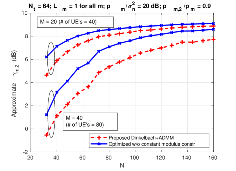
Figure 1: The approximate expected SINR for the weaker (IRS-assist) UE is shown with the number of IRS elements, $N$, for $M=20$ and $40$.

In the previous figure, we assume that the channel matrix for BS-IRS link $\bm{G}_{m}$ is full rank, which equals $\min\{N_{t},N\}$. In Fig. 2, we show how the rank of $\bm{G}_{m}$ can significantly impact the SINR. We fix $N=128$ and vary the rank of $\bm{G}_{m}$ for three different loads, $M=10$, $20$, and $30$. For a larger load, increasing the rank of $\bm{G}_{m}$ can sharply increase the optimized expected SINR. For $M=30$, the rank that achieves close to the maximum SINR is close to full. However, for $M=10$, the rank around $20$ can achieve close to the maximum. We also compare the SINR obtained from the proposed scheme in Algorithm 1 with that obtained without the constant modulus constraint. The two schemes perform similarly when the load is light or when the rank of $\bm{G}_{m}$ is very small or close to full.

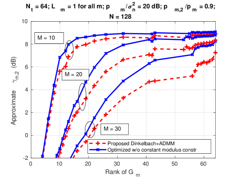
Figure 2: The approximate expected SINR for the weaker (IRS-assist) UE is shown with the rank of $\bm{G}_{m}$ for $M=10$, $20$, and $30$.

Fig. 3 shows the approximate rate of all UE’s with the total SNR, and is obtained from the proposed joint power-IRS element optimization scheme in Algorithm 2. For the minimum rate of 1 bps/Hz with $M=10$ and $N=128$, the total SNR required is about 13 dB. However, with doubling the load to $M=20$, the required total SNR is increased to about 20 dB. The larger increase in SNR is due to much larger interference power from the increasing load. If the number of IRS elements is reduced from 128 to 64, the required total power must increase by about 3 dB. However, we only observe a small power increase if the number of IRS elements is reduced to 96. For this figure, we assume full-rank $\bm{G}_{m}$ for all pairs. Thus, for a larger load, we expect a large increase in SNR if the rank of $\bm{G}_{m}$ is not full.

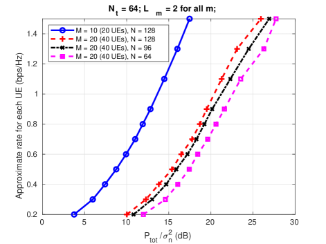
Figure 3: The approximate minimum rate for all UE’s obtained by Algorithm 2 is shown with the total SNR.

V Conclusions

We propose a low-complexity joint IRS-beamforming and transmit-power optimization that minimizes the total transmit power for a given rate threshold. The optimization is based on a long-term channel statistics instead of instantaneous channel coefficients. The performance of the IRS-assist UE’s significantly depends on the number of IRS elements and the rank of the channel matrix between the BS and IRS especially when the user load in the cell is heavy. The numerical results show that a few dB of the total transmit power can be saved when the number of IRS elements is doubled. The work demonstrates that IRS can be used to extend coverage and increase connectivity in cellular network.

References

- [1] Y. Liu, W. Yi, Z. Ding, X. Liu, O. A. Dobre, and N. Al-Dhahir, “Developing NOMA to next generation multiple access (NGMA): Future vision and research opportunities,” IEEE Wireless Commun., 2022, doi: 10.1109/MWC.007.2100553.
- [2] K. Mamat and W. Santipach, “On optimizing feedback-rate allocation for downlink MIMO-NOMA with quantized CSIT,” IEEE Open J. Commun. Soc., vol. 1, pp. 1551–1570, 2020.
- [3] Q.-U.-A. Nadeem, A. Kammoun, A. Chaaban, M. Debbah, and M.-S. Alouini, “Asymptotic max-min SINR analysis of reconfigurable intelligent surface assisted MISO systems,” IEEE Trans. Wireless Commun., vol. 19, no. 12, pp. 7748–7764, Dec. 2020.
- [4] G. Li, H. Zhang, Y. Wang, and Y. Xu, “QoS guaranteed power minimization and beamforming for IRS-assisted NOMA systems,” IEEE Wireless Commun. Lett., 2022, doi: 10.1109/LWC.2022.3189272.
- [5] X. Xie, F. Fang, and Z. Ding, “Joint optimization of beamforming, phase-shifting and power allocation in a multi-cluster IRS-NOMA network,” IEEE Trans. Veh. Technol., vol. 70, no. 8, pp. 7705–7717, Aug. 2021.
- [6] J. Qiu, J. Yu, A. Dong, and K. Yu, “Joint beamforming for IRS-aided multi-cell MISO system: Sum rate maximization and SINR balancing,” IEEE Trans. Wireless Commun., vol. 21, no. 9, pp. 7536–7549, Sep. 2022.
- [7] X. Liu, Y. Liu, Y. Chen, and H. V. Poor, “RIS enhanced massive non-orthogonal multiple access networks: Deployment and passive beamforming design,” IEEE J. Sel. Areas Commun., vol. 39, no. 4, pp. 1057–1071, Apr. 2021.
- [8] Y. Li, M. Jiang, Q. Zhang, and J. Qin, “Joint beamforming design in multi-cluster MISO NOMA reconfigurable intelligent surface-aided downlink communication networks,” IEEE Trans. Commun., vol. 69, no. 1, pp. 664–674, Jan. 2021.
- [9] M. Fu, Y. Zhou, Y. Shi, and K. B. Letaief, “Reconfigurable intelligent surface empowered downlink non-orthogonal multiple access,” IEEE Trans. Commun., vol. 69, no. 6, pp. 3802–3817, Jun. 2021.
- [10] W. Dinkelbach, “On nonlinear fractional programming,” Management Science, vol. 13, no. 7, pp. 492–498, 1967.
- [11] S. Boyd, N. Parikh, E. Chu, B. Peleato, and J. Eckstein, “Distributed optimization and statistical learning via the alternating direction method of multipliers,” Found. Trends Mach. Learn., vol. 3, no. 1, pp. 1–122, Jan. 2011.
- [12] Q. Li, C. Li, and J. Lin, “Constant modulus secure beamforming for multicast massive MIMO wiretap channels,” IEEE Trans. Inf. Forensics Security, vol. 15, pp. 264–275, 2020.
- [13] A. M. Sayeed and V. Raghavan, “Maximizing MIMO capacity in sparse multipath with reconfigurable antenna arrays,” IEEE J. Sel. Topics Signal Process., vol. 1, no. 1, pp. 156–166, Jun. 2007.
- [14] A. Adhikary, J. Nam, J.-Y. Ahn, and G. Caire, “Joint spatial division and multiplexing – The large-scale array regime,” IEEE Trans. Inf. Theory, vol. 59, no. 10, pp. 6441–6463, Nov. 2013.
- [15] T. Kim and S. Park, “Statistical beamforming for massive MIMO systems with distinct spatial correlations,” Sensors, vol. 20, no. 21, 2020, Art. no. 6255.
- [16] A. Zappone and E. Jorswieck, “Energy efficiency in wireless networks via fractional programming theory,” Found. Trends Commun. Inf. Theory, vol. 11, no. 3-4, pp. 185–396, Jun. 2015.
- [17] M. Schubert, “Power-aware spatial multiplexing with unilateral antenna cooperation,” Doctoral Thesis, Technische Universität Berlin, Fakultät IV - Elektrotechnik und Informatik, Berlin, Germany, 2003.
- [18] W. Yang and G. Xu, “Optimal downlink power assignment for smart antenna systems,” in Proc. IEEE Int. Conf. on Acoust., Speech and Signal Process. (ICASSP), vol. 6, Seattle, Washington, USA, May 1998, pp. 3337–3340.