mmFlexible: Flexible Directional Frequency Multiplexing for Multi-user mmWave Networks

Abstract

Modern mmWave systems have limited scalability due to inflexibility in performing frequency multiplexing. All the frequency components in the signal are beamformed to one direction via pencil beams and cannot be streamed to other user directions. We present a new flexible mmWave system called mmFlexible that enables flexible directional frequency multiplexing, where different frequency components of the mmWave signal are beamformed in multiple arbitrary directions with the same pencil beam. Our system makes two key contributions: (1) We propose a novel mmWave front-end architecture called a delay-phased array that uses a variable delay and variable phase element to create the desired frequency-direction response. (2) We propose a novel algorithm called FSDA (Frequency-space to delay-antenna) to estimate delay and phase values for the real-time operation of the delay-phased array. Through evaluations with mmWave channel traces, we show that mmFlexible provides a 60-150% reduction in worst-case latency compared to baselines.

I Introduction

Millimeter-wave (mmWave) networks have the potential to provide wireless connectivity to a growing number of users with their vast bandwidth resources. However, current mmWave systems have a significant limitation in that they are unable to simultaneously serve multiple users by distributing small chunks of frequency resources to different users who are in different directions. Unlike sub-6 systems, that use Omni-antennas to radiate signal in all directions, mmWave systems use pencil beams that illuminate a small region in space, meaning that all the frequency components are directed towards a fixed direction and cannot be distributed to other directions. This inflexibility leads to two main issues, as illustrated in Figure 1(a). Firstly, it leads to high latency, as the base station (gNB) must serve different user directions in a time-division manner, causing some users to experience long wait times, which is detrimental to latency-sensitive applications. Secondly, it leads to low effective spectrum usage. When a gNB serves one device at a time, each device gets a lot of instantaneous capacity which it may fail to utilize due to limited demand. But because the gNB cannot direct the remaining frequency resources in other directions, those resources are wasted, leading to low effective spectrum usage. Furthermore, other users in other directions could have used these wasted bands to improve overall spectrum usage.

In this paper, we ask the question “whether a mmWave base station can transmit or receive to any set of arbitrary directions using any set of contiguous frequency bands, creating a flexible frequency-direction beamforming response”. This is possible using massive antennas and digital beamforming, but traditional mmWave systems rely on analog phased arrays with a single RF chain for cost and power efficiency. However, analog phased arrays cannot create such a frequency-direction response, as they take a single input from the RF chain and radiate all frequencies in the signal in one fixed direction. One naive solution is to split the phased array into multiple sub-arrays and program them to radiate in different directions, but this reduces the directivity in each direction, reducing signal strength, range, reliability, and even data rate.

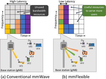
Figure 1: mmFlexible enables efficient use of the available mmWave spectrum resources through flexible directional-frequency multiplexing, allowing multiple users to be served simultaneously with low latency and high spectrum utilization.

Recently, new mmWave front-end architectures such as true-time delay (TTD) array [1, 2, 3] and leaky-wave antenna [4] have been proposed for frequency-dependent beamforming that spread different frequencies in different directions. However, these beam patterns have limitations in that each user only receives a tiny fraction of the bandwidth in one timeslot, which may not meet their demand in a reasonable time frame. Additionally, these architectures do not provide control over the number of beams, beam directions, and beam-bandwidth, resulting in large chunks of frequency resources being wasted in directions where there is no active user, leading to low spectrum utilization.

We propose a system called mmFlexible that performs flexible directional-frequency multiplexing by allocating a sub-set of contiguous frequency resources to each user, regardless of their direction, preventing spectrum wastage. This is achieved by creating multiple concurrent pencil beams (multi-beams) in different user directions, where each beam carries a separate frequency band according to the user’s demand in that beam direction. A key feature of mmFlexible’s multi-beam response is that it preserves beamforming gain across all beams while re-distributing power to only desired frequency-direction pairs with minimal leakage in other directions and frequency bands. This set of frequency-direction pairs can be chosen arbitrarily, providing flexibility in performing directional-frequency multiplexing. This enables efficient use of the entire frequency band (up to 800 MHz for 5G NR and 2.3 GHz for IEEE 802.11ax bands), reducing spectrum wastage and providing low latency network access, as shown in Fig. 1(b).

To implement mmFlexible, we introduce a novel mmWave analog array architecture called delay phased array (DPA) that can generate multi-beams with a flexible number of beams, with arbitrary beam directions and beam bandwidths (Refer to Figure 3). Unlike fixed delay architectures, DPA uses variable delay and phase elements at each antenna to create any desired frequency-direction response. Our insight is to use delays and phases in a complementary manner, with variable delay providing frequency selectivity and variable phase providing direction steerability, allowing DPA to create multi-beams towards multiple arbitrarily chosen frequency-direction pairs.

We architect the design of DPA and provide insights on the hardware requirements for creating the antenna array, and perform an analysis on the range and resolution of variable delay values required to generate our desired multi-beams. One of the challenges in implementing large delays on circuits is the size and complexity of the transmission lines, and integrating them onto an IC becomes even more difficult at mmWave frequencies due to bandwidth and matching constraints [5]. Our design addresses this by significantly reducing the range of delay values required, compared to traditional TTD array designs, making it practical and easy to manufacture. For example, TTD array requires monotonically increasing delays at each antenna, requiring a delay of 20 ns even for a 16-element array, which is 13x more than state-of-the-art mmWave delay designs [5]. In contrast, our DPA design consists of increasing and decreasing delay values for consecutive antennas, resulting in lower delay range requirements than traditional TTD arrays. Furthermore, the delay range is independent of the number of antenna elements, making it scalable for large arrays.

The next challenge is the software programming of DPA to meet the beamforming requirements of mmFlexible. The software should determine the appropriate values for the variable delays and phases at each antenna of DPA. Solving for these discrete values is computationally difficult as it is a non-convex and NP-hard problem. A naive solution is to pre-compute and store the delay and phase values for every possible frequency-direction pair, but this is infeasible due to a large number of such combinations ($10^{28}$). To overcome this, we develop a novel FSDA (frequency-space to delay-antenna) algorithm which provides a single-shot solution for estimating the delays and phases in real-time. It does this by mapping the desired frequency-space response to the delay-antenna space using a 2D transform and then extracting the corresponding delays and phases for each antenna. FSDA algorithm can be implemented in real-time using fast and efficient 2D FFT techniques. Our algorithm only requires the angles for each user and corresponding frequency resources allocated to users in the current time slot. The angles can be obtained from any standard compliant initial access protocol and so mmFlexible can be easily integrated into the standard 5G mmWave protocols.

In summary, we make the following contributions:

• We propose mmFlexible, the first system that enables flexible directional-frequency multiplexing in mmWave networks, achieving higher spectrum usage, low latency, and scalability to support a large number of users.

• We design a novel mmWave front-end architecture called delay phased array that can generate multi-beams with a flexible number of beams, beam directions, and beam-bandwidths while maintaining high beamforming gains.

• We provide a new algorithm called FSDA (Frequency-space to delay-antenna) which estimates delays and phases in real-time using 2D FFT techniques and can be easily integrated with standard 5G mmWave protocols.

• We evaluate the performance of mmFlexible using real mmWave traces and show an improvement in latency by 60-150% compared to baselines. Furthermore, the multi-user sum-throughput is improved by 3.9x compared to true-time-delay array baseline [1].

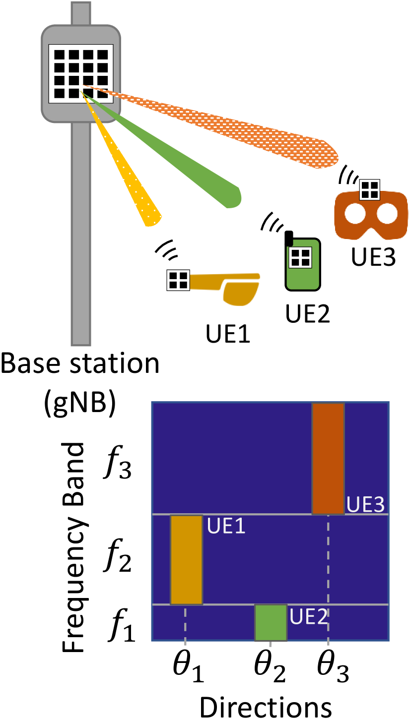
Figure 2: Desired frequency-space beam response for 3 users in 3 different angular directions.

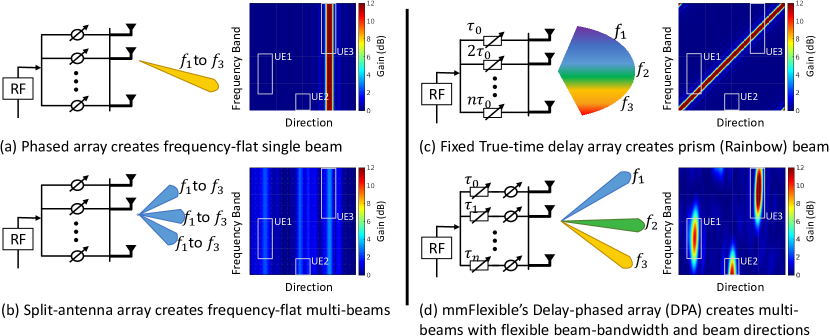
Figure 3: Comparison of different mmWave front-end architectures and corresponding frequency-space patterns they created. The traditional phased array and split-antenna array create a frequency-flat response, while TTD array creates a frequency-selective rainbow-like pattern radiating in all directions. In contrast, DPA provides a flexible frequency-direction response with a programmable number of beams, beam-bandwidth, and beam directions.

II Background and Motivation

In this section, we would provide a primer on different analog antenna array architectures, which have a single baseband radio frequency (RF) chain and mechanism to best achieve flexibility in resource allocation to multiple users. Next, we would show a realistic example (Figure 3) that none of the architecture can meet the requirements for flexible directional-frequency multiplexing, and how our flexible DPA architecture can meet these requirements.

II-A Primer on phased arrays and true-time delay arrays

$\blacksquare$ Phased array: The phased array takes a single input from the digital chain, split into $N$ copies, apply appropriate phase-shift, and radiates from $N$ antennas (Fig. 3(a)). The input signal with all of its constituent frequency bands is radiated in a direction specified by the phase setting. The set of phases at each antenna constitutes a weight vector $w_{\text{phase}}$ as:

$$w_{\text{phase}}(n)=e^{j\Phi_{n}}$$ (1)

where $\Phi_{n}$ is the programmable phases for antenna index $n(n\in[0,N-1])$. Now, if we program the phases to create a directional beam at an angle say 30^∘, then this phase shift is applied to all the frequency components in the signal radiating them along that same angle 30^∘. Different frequency components in the signal cannot be radiated to other directions because of the frequency-independent nature of weights in a phased array. Therefore, a phased array can serve users in only one direction at a time and cannot perform flexible directional-frequency multiplexing with many users. Split-antenna phased array (Fig. 3(b)) uses the phased array architecture split into multiple sub-arrays to create multiple beams towards different users in one TTI, but suffers from lower antenna gain, range, and throughput.

$\blacksquare$ True-time delay array: The true-time delay (TTD) array uses a delay element to replace the phase shift element as shown in Fig. 3(c). The antenna weights with delay element is given by:

$$w_{\text{delay}}(t,n)=\delta(t-\tau_{n})$$ (2)

Past work on TTD array [2, 6, 3, 1] have shown that this architecture creates a prism-type response by radiating all the frequencies in all the directions in a linear fashion (Fig. 3(c)) by using a fixed set of delays at each antenna given by $\tau_{n}=\frac{n}{\text{B}}$, for bandwidth $B$. This response has two major limitations: 1) most frequency bands would be wasted in space if there are no user in that direction and 2) each user gets a small frequency band and cannot scale it up arbitrarily. Due to these limitations, TTD array is not suitable for flexible directional-frequency multiplexing.

II-B Current mmWave architectures are incapable for flexible directional-frequency multiplexing

Let us take a simple network scenario to understand the performance tradeoffs for the above systems. Typically for 4K VR applications, end-end latency should be $<100$ ms, Where transmission goes from the public cloud, network provider, base station (edge), and device. Over-the-air (base station to device) transmission latency comes down to a strict latency requirement of $<1$ ms [7]. Consider 10 users in the network with similar traffic demand: each user requires 60 Mbps (4K VR) throughput and $<1$ ms over-the-air latency due to the interactive nature of VR [8, 9, 7, 10]. The aggregate throughput provided by the users is 600 Mbps, only 30% of the max physical layer throughput of a 400 MHz FR2 gNB in downlink (2.2 Gbps). We assume all users are distinctly located (in different angular directions) and RF conditions are good (e.g. LOS and no blockage). This allows us to control common external factors and exclusively evaluate architectural capabilities. We assume our DPA and split array can create up to 8 concurrent beams and TTD array creates a prism beam pattern. The comparison is shown in Table I. From our end-end evaluations (Fig. 7(a)), we can see that in edge scenarios all the baselines failed to meet the $1$ ms over-the-air latency requirement. It is evident that mmFlexible is the best to support latency-critical applications while satisfying higher throughput demands.

Architecture	Latency* (ms)	Packet Loss	Throughput
phased array (TDMA)	$>1.25$ ms	24.0%	54.9 Mbps
split-antenna array	$>2$ ms	33.3%	47.3 Mbps
TTD array	$>3.5$ ms	76.4%	18.3 Mbps
DPA	$<0.5$ ms	0.0%	71.3 Mbps

TABLE I: Delay-phased array & other baselines for 10 4k VR users (*We mention over-the-air worst case latency).

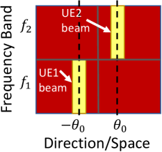
(a) Desired F-S image

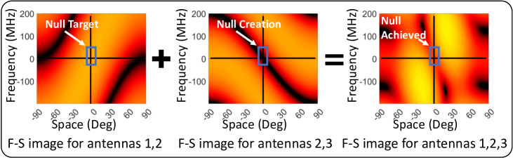
(b) Specific Frequency-Space (F-S) signature images

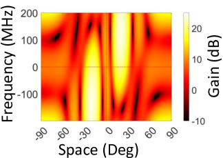
(c) 8 antenna F-S image

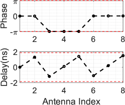
(d) Delays and phases

Figure 4: Explanation on how DPA creates a desired frequency-space image with two beams at $-20^{\circ}$ and $20^{\circ}$. The first beam occupies a frequency band in [-200,0] MHz and the second beam occupies a frequency band of (0,200] MHz. DPA can create the desired image in (c) using delay and phase values in (d).

III mmFlexible’s DPA hardware design

mmFlexible introduces a new mmWave front-end architecture, delay-phased array (DPA), to enable flexible directional-frequency multiplexing for mmWave networks. The DPA design addresses the limitations of existing mmWave systems with phased arrays and TTD arrays by creating a multi-beam response with flexible beam directions and beam bandwidths. In this section, we discuss the practical implementation of DPA and show how we can build it with shorter delays.

III-A Architecture of delay-phased array (DPA)

DPA architecture consists of programmable delay and programmable phase element per antenna with a single-RF chain as shown in Fig. 3(d). These elements can be programmed together to create flexible beam responses that are not possible by either of the two elements alone. Our insight is to control two knobs: delays $\tau_{n}$ and phase $\Phi_{n}$ to get the desired response. We define beam weights for DPA as:

$$w_{\text{dpa}}(t,n)=w_{\text{phase}}(n)w_{\text{delay}}(t,n)=e^{j\Phi_{n}}\delta(t-\tau_{n})$$ (3)

Notice the dependence of DPA weights with time, which leads to a dependence on frequency. Upon taking FFT, the exponential term in the weights become $\Phi_{n}-2\pi f\tau_{n}$, which is a function of frequency $f$ at antenna index $n$. Therefore, the beamforming response of this weight vector will be a function of both frequency and direction. The beamforming gain of an antenna array represents the power radiated by the antenna array in different directions. The expression for beamforming gain $G(f,\theta)$ for DPA at a frequency $f$ and direction $\theta$ is:

$$\begin{split}G(f,\theta)&=\sum_{n=0}^{N-1}\mathcal{F}(w_{\text{dpa}}(t,n))e^{-jn\pi\sin(\theta)}\end{split}$$ (4)

where $\mathcal{F}$ is Fourier transform and $e^{-jn\pi\sin(\theta)}$ is the standard steering vector transformation from the antenna to space ($\sin(\theta)$)-domain. Essentially, the response is the sum of the individual contribution from all antennas. By equating exponential terms of DPA weights to that of array response, we get: $\Phi_{n}-2\pi f\tau_{n}=n\pi\sin(\theta)$. The variable delay causes a slope in frequency ($f$) - space ($\sin\theta$) plot, while the variable phase causes a constant shift along the space axis. Together, they can create an arbitrary line with a configurable slope and intercept in the frequency-space domain. With this insight in place, we will discuss how to program the phase and delay values at each antenna to get the desired beam response in Section IV.

III-B Range of delay element in DPA

Before discussing DPA software programming, we emphasize that it is important to analyze the set of possible delay values that the hardware can support practically. Here we describe the requirements for the delay range and how it helps create a practical circuit board. Delay elements are implemented with variable-length transmission lines on a circuit board. Building large delay lines in IC at mmWave frequencies is prohibitive because of large size, bandwidth, and matching constraints [5]. Therefore, our design ensures that the delay range is not too large. While traditional true-time delay (TTD) array requires a delay range proportional to the number of antenna $N$, which is large for large antenna array (18.75 ns for 16 antenna array) [1]. In contrast, the delay range for mmFlexible is independent of the number of antennas. For the two-beam case, the delay range for mmFlexible is $\frac{3}{2B}$ (shown later in (5)), which is $3.7ns$ for 400 MHz bandwidth for 5G NR; significantly less than that required by TTD arrays. The delay range increases with the number of concurrent beams, but is independent of the number of antennas, making it scalable to large arrays.

Delay control with sub-ns accuracy has been demonstrated in full-duplex circuits for interference cancellation [12]. Recently, authors of [13] have shown accurate delay control with 0.1 ns resolution and with 6-bit control (64 values until 6.4 ns), which satisfies the requirement of mmFlexible.

IV mmFlexible’s DPA Software Design

IV-A Requirements for mmFlexible

Our goal is to construct arbitrary frequency-direction response $G(f,\theta)$ via DPA architecture, which would be energy efficient and enable efficient resource utilization with low latency. If we carefully notice the example in section 2, we observe that the split antenna achieves the frequency-direction mapping but with a loss of 6 dB SNR, which is a corollary of the entire 400 MHz radiated in each of the four directions. It leads to our first requirement: Req.1: The system must be able to transmit/receive signals in the specific frequency-direction pairs associated with each user, with minimal energy leakage in other directions and frequencies. Furthermore, we should be able to control the amount of bandwidth assigned to each user, which leads to: Req.2: Flexibility in allocating bandwidth to each user, allowing for narrow beams in space for higher antenna gain and wide beams in frequency to support high-demand users.

IV-B Meeting mmFlexible’s requirements with DPA

With this intuition in place, we revisit and explain how can mmFlexible achieve these requirements through a simple two-user example in Fig. 4. Let us consider the two users are located at $-\theta_{0}$ and $\theta_{0}$ respectively, and the base station wishes to serve these two users with equal beam-bandwidth of $B/2$ each, where $B$ is the total system bandwidth. To support such flexible directional-frequency multiplexing, the base station must create a frequency-direction beam response shown in Fig. 4(a). We call such 2D beam patterns as frequency-space (F-S) images for simplicity. So how does DPA create these images and meet the above requirements?

We provide a closed-form expression for the set of delays $\tau_{n}$ and phases $\Phi_{n}$ for each antenna that would generate the above beamforming response as follow:

$$\tau_{n}=\left(\frac{3}{2B}n\sin(\theta_{0})+\frac{3}{4B}\right)\;\;\;\text{mod }\frac{3}{2B}$$ (5)

$$\Phi_{n}=\text{round}(n\sin(\theta_{0}))\pi\;\;\;\text{mod }2\pi$$ (6)

A more generalized expression for an arbitrary number of beams, beam directions, and beam bandwidth along with their proof can be found in Appendix -A.

Now, we achieve the requirements for mmFlexible by assigning a complementary F-S images to a subset of antennas. For instance, we create a positive slope in F-S image using antennas 1 and 2, and then create a complementary negative slope with antenna 2 and 3 as shown in Fig. 4(b). When the two responses are combined together, we observe a frequency-space image where they combine constructively at desired user locations while creating a null (low gain) at other locations (Meeting Req-1).

For the second requirement, we create such beams by choosing the number of antennas for creating a positive or negative slope. The intuition is that a higher number of antennas makes the corresponding signature image narrow in space. For instance, it is clear from Fig. 4(d) that three consecutive antennas (e.g. antenna 3,4,5) have increasing delays, while only two antennae (e.g. 2,3) have decreasing delays. This helps in making the positive slope in the F-S image narrow (3 antenna contribution), while the negative slope remains wide (2 antenna contribution). This effect causes beams that are narrow in space, but arbitrarily wide in frequency as shown in Fig. 4(c) (Meeting Req-2).

This intuition helps in understanding how a simple 2-beam frequency-space image is created. We use this insight to develop a novel FSDA algorithm that estimates the delay and phase values for any frequency-space image with an arbitrary number of beams, beam directions, and beam-bandwidths.

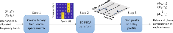
Figure 5: Three steps of our FSDA algorithm to estimate per-antenna delays and phases that generate a desired frequency-space image. The core step is our novel 2D FSDA transform with some pre-processing and post-processing of inputs and outputs respectively.

IV-C FSDA algorithm for estimating delays and phases in DPA

To create a desired frequency-direction beam response, the base station needs to estimate the corresponding delays and phases per-antenna in DPA. One naive solution is to try different discrete values in a brute-force way using a look-up table to get the desired beams. But, this solution is computationally hard and memory intensive since there is a large set of possibilities for the delays and phases at each antenna. For instance, with 64 delays and 64 phases per antenna (assume both are 6-bit, so $2^{6}=64$), a brute-force look-up table search would require $64^{N}\times 64^{N}\approx 10^{28}$ probes to try each combination and then storing it all in memory, which is impossible to solve with even high memory and high computing machines. Our insight is that we can pose this problem as an optimization framework and solve them in a computationally efficient way.

We now formulate the optimization problem with insights we have obtained from the previous subsection and from the fundamentals of digital signal processing. The goal is to relate weights (delays and phases) to the antenna gain pattern in (7) in a way that simplifies our estimation problem.

Our insight is that similar to how frequency and time are related by a Fourier transform, there is a similar transform that relates space and antenna using steering matrices. So, there are two transforms that bridges the world of antenna weights to the desired gain pattern: time to frequency transform and antenna to space transform. Mathematically, we re-write the gain pattern of DPA to emphasize this 2D transform:

$$G(f,\theta)=\sum_{k=0}^{K-1}\sum_{n=0}^{N-1}\mathbf{U}(f,k)w_{\text{dpa}}(k,n)V(n,\theta)$$ (7)

where $\mathbf{U}(f,k)$ is a discrete domain Fourier transform (DFT) and the steering matrix $V$ is defined per-element as $V(n,\theta)=e^{-jn\pi\sin(\theta)}$. Now since the signal is actually sampled only discretely with a sampling time of $T_{s}$, our original delay weight element $w_{\text{delay}}(t,n)$ would reduce to $w_{\text{delay}}(k,n)=\delta(kT_{s}-\tau_{n})$ as described in (7).

We then represent the gain pattern by a discrete frequency-space matrix $\mathbf{G}$ and the weights as discrete time-antenna matrix $\mathbf{W}$ and relate them with the following 2D transform:

$$\mathbf{G}=\mathbf{U}\mathbf{W}\mathbf{V}$$ (8)

where $\mathbf{U}$ is time to frequency transform matrix and $\mathbf{V}$ is antenna to space transform matrix. Here we formulate $\mathbf{W}$ as $K\times N$ matrix, where $K$ is the number of discrete time values and $N$ number of antennas.

We follow a three-step process to estimate the weight matrix $\mathbf{W}$ that creates our desired frequency-space image intuitively explained in Fig. 5. There are two inputs to our algorithm: Angles and desired frequency bands for each user. These two inputs are enough to represent the given frequency-space image. As a first, we create a binary frequency-space matrix that consists of 1s at desired frequency-space locations and 0s otherwise, we denote it by $\mathbf{G}_{\text{desired}}$. We then formulate the following optimization problem:

$$\begin{split}\hat{\Phi_{n}},\hat{\tau_{n}}&=\min||\mathbf{G}_{\text{desired}}-\mathbf{U}\mathbf{W}\mathbf{V}||^{2}\\ \text{s.t.}\quad&\mathbf{W}(k,n)=e^{j\Phi_{n}}\delta(kT-\tau_{n})\end{split}$$ (9)

This optimization is a non-convex due to the non-linear terms such as exponential in phase and delta in delay. Moreover, the constraint of having a discrete set of values for delays and phases makes it NP-hard. We make an approximation by relaxing the delta constraint and letting the weights at each antenna take any variation over time. It means that we allow weights to take the form of a continuous profile over time at each antenna rather than a delta function which is non-zero at only one value and zero otherwise. We call it the delay-phase profile at each antenna. How do we estimate this delay-phase profile?

Our insight is that we can write an inverse transform of $\mathbf{U}$ and $\mathbf{V}$ to go from the frequency-space domain to the time-antenna domain. The logic behind such formulation is that using an appropriate discrete grid along the time and space axis, we can formulate $\mathbf{U}$ and $\mathbf{V}$ as linear transforms, i.e., $\mathbf{U}^{\dagger}\mathbf{U}=\mathbf{I}$ and $\mathbf{V}\mathbf{V}^{\dagger}=\mathbf{I}$ for identity matrix $\mathbf{I}$ (Note $(.)^{\dagger}$ is pseudo-inverse of a matrix). Therefore, it is easy to write their inverse by simply taking the pseudo-inverse. We estimate $\hat{\mathbf{W}}$ as:

$$\hat{\mathbf{W}}=\mathbf{U}^{\dagger}\mathbf{G}_{\text{desired}}\mathbf{V}^{\dagger}$$ (10)

The final step of our algorithm is to extract delays and phases from $\hat{\mathbf{W}}$. Note that each column in $\hat{\mathbf{W}}$ contains the delay-phase profile. We find the maximum peak in this profile and the index corresponding to this peak gives the delay and the max value at this peak gives the phase term. Note that since we did not put any restriction on the number of non-zero delay taps, we could get more than one delay tap per antenna. We empirically found that the estimated delay profile has only one significant peak with high magnitude than other local peaks (See Section V). Also, the intuition comes from our insights from the previous section that usually one delay per antenna suffices in creating the desired response.

$\blacksquare$ Weights Quantization: The delay and phase values obtained from FSDA algorithm are still continuous in nature and must be discretized to be fed into the DPA hardware. We quantize both the phase and delay values with a 6-bit quantizer in software before feeding to the array. The quantized phase takes one of the 64 values in $[0^{\circ},360^{\circ})$ and the quantized delay varies in the range [0, 6.4ns) with an increment of 0.1 ns.

$\blacksquare$ Computation complexity of FSDA: The run-time complexity of FSDA is dominated by the 2D FFT transform on a given frequency-space image. Given the frequency, the axis is divided into $M$ subcarriers and the space axis into $D$ directions, the run-time complexity is ${\mathcal{O}}{(MD(\log(M)+\log(D))}$.

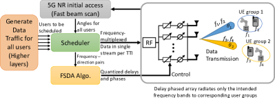
Figure 6: Implementation overview for mmFlexible with four main components: Data traffic generator, Fast beam scan angle estimation, a scheduler, and our FSDA algorithm.

V Evaluation

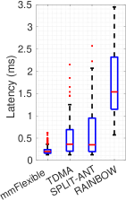
(a) Latency

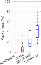
(b) Loss for $<$1ms latency

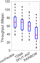
(c) Thput for $<$1ms latency

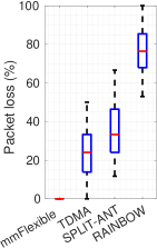
(d) Loss for $<$0.5ms latency

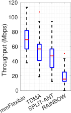
(e) Thput for $<$0.5ms latency

Figure 7: End to End performance gain with DPA compared to baselines under different scenarios: (a) mmFlexible is able to meet strict latency constraints ($<$ 1 ms), but the baselines are not; (b) to (d) Percentage of packet loss and Throughput performance for latency constraint $<$ 1 ms and $<$ 0.5 ms respectively.

V-A Implementation and emulation with 28 GHz dataset

We implement an end-end system of mmFlexible with four major components, as illustrated in Fig. 6. The components of the systems are as follows:

1. Data traffic generator: We generate MAC layer packets with the throughput and latency constraints mentioned in the example in Sec. II based on [10, 9, 7]. We test with two different latency constraints: 1 ms and 0.5 ms. We use the same traffic generator for our system and all baselines.

2. Users angle estimation (initial access): We use the channel collected from mobile 28 GHz testbed [14], using switched beamforming techniques [15, 16] for user’s angle estimation. We leverage the existing 5G NR SSB Beam scan [17] using an exhaustive search to estimate angles. The gNB scans 64 beams in the codebook, and each UE reports the best beam index that maximizes the received signal strength from which the gNB determines the user’s angle.

3. Data Scheduling: We implement a Proportional Fair (PF) scheduler [18] to allocate spectrum resources to users on a per-TTI basis. The available $120^{\circ}$ field of view is mapped into 10 groups with each $12^{\circ}$ half-power beam width. The scheduler uses user grouping, demand generation information, and SNRs (mapped to CQIs) to determine which user group to support and how many subcarriers to allocate for each user. Throughput is then calculated as a function of the allocated resources and channel to each user.

4. FSDA Algorithm: Our system’s front-end uses DPA, requiring delays and phases as input. The FSDA algorithm provides quantized delays and phases, which are applied to the DPA to generate beams in desired directions and frequency bands. Array gain from the FSDA algorithm or respective baselines is then fed back to the scheduler for SNR computation.

We evaluate the performance of the baselines and mmFlexible with a PF scheduler by emulating $2000$ TTIs of $125\mu s$ each, for a total duration of 0.25 seconds, across all users. The system undergoes the above four-step procedure for each TTI.

$\blacksquare$ Baselines: Our paper compares the performance of mmFlexible with three baselines: TDMA, Split antennas [19], and Rainbow-link [1]. The TDMA approach has the scheduler assign one direction per TTI and beam in that direction over all frequencies. The Split antennas baseline has the scheduler assign one or multiple directions based on SNR & demand requirements support the given directions in all subcarriers. The Rainbow-link [1] transmits in all directions regardless of the number of user directions, using only subcarriers in user directions and wasting the rest.

V-B End-to-end Results

1) Latency: Latency is the time for a packet to travel from source (gNB) to destination (UE) over the air. We evaluate the latency distribution across the baselines and present the results in Fig 7(a). We see that mmFlexible has a median latency of 0.2 ms, while TDMA and Split-antenna baselines have a higher median latency of 0.32 ms and 0.26 ms respectively. Our implementation features equal offered throughput for every user direction, which is the best case scenario for Rainbow-link operation; despite this, the median latency for the Rainbow-link is 1.5 ms because of its inability to assign bandwidth to a user that is proportional to its demand. The worst-case latency of mmFlexible is well below 1 ms. Notably, all baselines have weighted right tail distributions of latency, making their worst case much worse than 1 ms. The inability of the baseline methods to honor the latency constraint leads to dropped packets and ultimately lower link throughput and reliability.

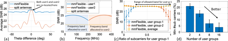
Figure 8: The benchmark performance gain of mmFlexible compared to baselines under different scenarios: (a) Angle separation between two users (b) (c) Subcarrier allocation between users (d) How much minimum frequency resources can be allocated without SNR degradation.

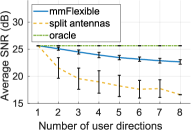
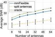
Figure 9: Scaling the mmFlexible’s performance with (a) Increasing number of user directions and (2) Increasing number of antennas.

2) Packet loss: If a packet’s latency constraint is not met, then the packet is considered undelivered and lost. In Fig 7(b) and Fig 7(d), we see that mmFlexible is able to function without any packet loss. However, due to their inability to honor the latency constraints, TDMA, Split-antenna, and Rainbow-link baselines result in a median packet loss of 24.0%, 33.3%, and 76.4% respectively. mmFlexible’s ability to serve multiple users in different directions enables it to optimally allocate resources without any power degradation and meet both throughput and latency constraints. TDMA is forced to serve one use direction at a time, resulting in a violation of latency constraints. Split-antenna baseline attempts to serve users in multiple directions simultaneously, but suffers from reduced throughput due to SNR degradation, resulting in high latency and packet loss compared to mmFlexible and TDMA. The Rainbow-link baseline allocates too few resources to each user and is the slowest and most unreliable in delivering packets.

3) Per-user Throughput: As shown in Fig.7(c) and Fig.7(e), mmFlexible outperforms all three baselines TDMA, Split antennas, and Rainbow-link. TDMA can only support one user group direction out of all the presented user demand directions, reducing its efficiency. However, in scenarios with heavy throughput demand, it performs similarly to mmFlexible. The mean throughput of mmFlexible is 1.3$\times$ that of TDMA throughput in the case of 0.5 ms latency requirement. The Split-antenna approach serves users in different directions by splitting its antennas, resulting in reduced overall throughput. mmFlexible provides 1.5$\times$ more throughput than the split scenario. Rainbow-link performs better only in scenarios with low throughput demand and users in all directions, but performance degrades in all other cases. mmFlexible provides 3.9$\times$ more throughput than the Rainbow-link baseline.

V-C Benchmarks

We benchmark various theoretical and systems aspects of mmFlexible and compare the results with a split-antenna baseline. We chose the split-antenna baseline as it is closest to mmFlexible in creating multiple simultaneous beams in different directions. We present our results by calculating SNR for various scenarios. We use a channel dataset (28 GHz testbed [14]) and compute SNR per user for all subcarriers by evaluating over LOS channel model [20] with no blockage and equal distance consideration for all users.

1) Effect of angular separation between users on SNR: We evaluate the performance of mmFlexible and a split-antenna approach in serving two users in different locations $(\theta_{1},\theta_{2})$ with a single RF chain and an equal number of subcarriers. Figure 8(a) shows the mean SNR of the two users for different angular separations $(\theta_{1}-\theta_{2})$. We observe that mmFlexible performs optimally in all cases compared to the baseline. When the angular separation is close to zero, both users are in the same direction and can be served by a single beam. In these scenarios, both approaches converge to a single beam and perform similarly. The baseline becomes inefficient as the angular separation increases, while mmFlexible provides a stable response after $12^{\text{o}}$ separation with a 3-5 dB higher gain than the baseline approach.

2) Does mmFlexible have interference due to multiple user transmissions from different directions? No, mmFlexible is designed to support frequency multiplexing of users in different directions without interference. We evaluated this by comparing mmFlexible to a split-antenna baseline for two users separated by $30^{\text{o}}$ angle and equal bandwidth, as shown in Fig. 8(b). Both approaches receive data from user-1 in the 0-200 MHz bandwidth and from user-2 in the remaining 200-400 MHz bandwidth, without sharing any subcarriers between users. This results in no interference from simultaneous multiple-user transmissions for both approaches. Additionally, mmFlexible provides a higher gain to users by radiating only in allocated subcarriers as illustrated in Fig. 3(d), resulting in higher SNR than the baseline. The average SNR over all subcarriers shows that mmFlexible has a gain of  5dB compared to the split-antenna approach, even a 3dB higher gain at edge subcarriers.

3) Impact of subcarrier allocation on SNR: mmFlexible can reliably support both low-bandwidth Ultra-Reliable Low-Latency Communication (URLLC) and high-bandwidth AR/VR devices in different directions simultaneously. Here we evaluate the effect of subcarrier allocation on SNR for two user groups. Fig.8(c) shows the SNR achieved with subcarrier allocation to user group-1 from 1% to 99% (remaining subcarriers are allocated to user group-2). The average SNR over all users remains at 25 dB and does not depend on the proportion of subcarriers allocated to individual user groups. It is observed that the SNR of user group-1 converges to the average SNR when it is allocated more than 20% of the total subcarriers. Therefore, to achieve the benefits of mmFlexible in a URLLC link, at least 20% of the total subcarriers should be allocated to a user group. Additionally, as presented in Fig.8(d), as the number of user groups or user directions increases, the convergence point occurs at a lower percentage of subcarriers allocated. For instance, when there are 4 users in the system, then each user can be allocated with a minimum 15% of subcarriers without degrading the SNR performance. This convergence point drops down to 4% for 16 users which is favorable for URLLC applications which requires low-bandwidth and low latency.

Theoretical Baseline (Oracle): Oracle is a theoretical entity that can perfectly transmit only in desired subcarriers without any degradation in power at edge subcarriers (as shown in Fig. 3 desired frequency-space response).

4) Impact of the number of user directions: The performance of the mmFlexible improves as the number of supported user directions increases. We tested the system using a base station antenna array with 8 transmit/receive antennas, varying the number of user directions from 1 to 8. Fig. 9 illustrates that the relative gain (difference between the average SNR of mmFlexible and split antennas) increases with an increase in user directions. As the number of user directions increases, the split antenna approach divides the antennas per beam, resulting in reduced gain. Conversely, mmFlexible transmits power only in desired frequency bands and angular directions resulting in a higher gain. The Oracle creates a digital frequency filter at each antenna, resulting in a perfect frequency-space slicing which ensures that the average SNR remains constant regardless of whether it serves in one direction or multiple directions simultaneously. In contrast, mmFlexible has one delay per antenna (for hardware feasibility), which makes it difficult to create an ideal frequency-space slicing, leading to power degradation at the edge subcarriers. Despite this, even after eight splits, the degradation is less than 2.5 dB with the Oracle, and the gain is more than 6 dB higher compared to the split antenna baseline. Error bar in Fig. 9 indicates average SNR variations with users in different angle separations.

5) Impact of the number of antennas: We show that mmFlexible performs better with the increase in the number of antennas. We evaluated this hypothesis by serving four users and varying antennas from 8 to 64. Fig. 9 shows gain variations from 8 antennas to 64 antennas for 4 users; it is clearly evident that mmFlexible outperforms with the increase in antennas over the split antennas baseline. The error bar in the figure shows the variations in the average SNR when serving four users at different angle separations. Similar to the Oracle, mmFlexible’s performance remains constant even as the number of antennas increases because the number of frequency splits is determined solely by the number of user directions, which are the same in all cases.

VI Related Work

mmFlexible builds upon previous work in mmWave and THz communications, but sets itself apart by introducing a system that can perform flexible directional-frequency multiplexing, while maintaining energy efficiency and high performance in terms of range, throughput, and link reliability. To the best of our knowledge, no existing literature has achieved this level of frequency slicing without compromising on performance. mmFlexible’s unique approach enables efficient use of the entire frequency band, reducing spectrum wastage and providing low latency network access.

$\blacksquare$ Split antenna phased array: Traditional phased array beamforming does not support flexible directional-frequency multiplexing because of a single narrow pencil beam. In the past, split-antenna arrays have been used to create concurrent multi-beams across multiple directions [21, 22, 23, 24, 25]. However, this approach often results in lower beamforming gain and throughput for each user. The array gain reduces proportionally to the number of beams as the total available power is distributed along multiple directions and across the entire bandwidth. In contrast, mmFlexible uses a unique split-beam mechanism with frequency selectivity that radiates only in the desired frequency band, preserving high directivity, signal strength, and throughput.

$\blacksquare$ True-time delay array architecture: Previous work on True-time delay arrays (TTD) has primarily focused on beam steering for ultra-wideband signals [26, 27] and, more recently, single-shot beam training [2, 28, 3], compressive channel estimation [29], wideband tracking [30] and THz communication [31]. However, none of these works address the problem of flexible low-latency multi-user communication. Rainbow-link [1] uses TTD arrays for multi-user communication, but it is limited to fixed low-throughput IoT applications (limited to 7.8 MHz per user [1]) and cannot flexibly allocate a large number of subcarriers to a single direction for broadband users. mmFlexible addresses this limitation by using variable delay elements to create arbitrary frequency slicing and the ability to radiate those frequencies in any desired direction. mmFlexible’s beamforming is orthogonal to previous work in this area, but it can leverage the fast beam training capability of TTD arrays.

Recently, a new approach called Joint Phase-Time Array (JPTA) has been proposed for creating frequency-dependent beams [32] that is similar to mmFlexible in its goals. However, mmFlexible and JPTA have several key differences in their implementation and performance. Firstly, JPTA does not provide any details on the specific hardware architecture and the range of delay values required to support their beamforming patterns. mmFlexible is the first work that provides a clear explanation of the DPA hardware architecture and the range of delay values required to support our beamforming patterns. We have shown that our DPA patterns can be realized with shorter delays and independent of the number of antennas making it practical and realizable with current technology, and scalable to large antenna arrays. Secondly, JPTA requires digital processing over each frequency subcarrier, while DPA programming is fully analog and does not require any digital programming over the frequency subcarriers. Finally, JPTA has a high run-time complexity for estimating the delay values which makes it inadequate for real-time operation, while mmFlexible provides a closed-form mathematical expression for delays that can be used as plug-and-play with a constant run-time complexity.

$\blacksquare$ Other front-end mmWave architectures: In [33], a new mmWave receiver architecture for frequency multiplexing was proposed, which utilizes a network of mixers at each antenna to receive different frequency components from different directions. However, this approach has a fixed hardware structure that is not scalable to support a large number of users, requiring different hardware for different numbers of users. In contrast, mmFlexible’s delay-phased array (DPA) is flexible and programmable, providing a scalable solution for supporting a large number of users.

VII Discussion and Future Work

We discuss potential future work ideas:

$\blacksquare$ Circuit for DPA: Implementing circuit delays in mmWave frequencies is challenging due to non-linearity, bandwidth and matching constraints [34, 35]. In contrast, delay elements can be more accurately implemented at intermediate frequencies (IF) (sub-6 GHz) using techniques such as voltage-time converters [13] and switched-capacitor arrays [5]. Recent work [5] has shown that efficient mixers, phase-shifters, and IF true-time-delays can be used to make a DPA that meets the requirements of mmFlexible.

$\blacksquare$ Single RF vs Multi-RF systems: mmFlexible works with a single-RF chain and radiating each frequency component in different directions, while past work on the single-RF system stream all frequencies in one direction. Multi-RF systems (Hybrid arrays) [36, 37] offer freedom to create multi-stream to multi-directions, but each stream carries the entire bandwidth. Thus they also cannot perform flexible directional-frequency multiplexing. Our work can be extended to the multi-RF system where each RF is connected to a DPA that creates large sectors where each DPA can serve in a sector with our flexible directional-frequency multiplexing technology.

$\blacksquare$ Applications beyond flexible frequency multiplexing: Delay-phased arrays have the potential to enable a plethora of applications in communication and sensing beyond flexible directional-frequency multiplexing. For instance, the ability to create arbitrary and controllable frequency-space beams can help faster localization and tracking of multiple targets. Delay-phased arrays also enable simultaneous communication and sensing paradigms where some frequency bands are used for communication while other bands can be used for sensing. All these applications can be enabled with simple software or firmware updates on the same underlying hardware. We leave these applications for our future work.

VIII Acknowledgements

We are grateful to the anonymous reviewers their valuable feedback, as well as to the WCSNG group at UC San Diego for their input. The research was supported by NSF #2211805.

-A Generalized closed-form delay and phase expression

In this section, we propose a closed-form mathematical expression for the delays and phases that can be used to generate a desired multi-beam pattern with DPA. This approach eliminates the need for complex computation and allows for real-time operation with run-time complexity reduced to ${\mathcal{O}}(1)$. Additionally, this mathematical expression also provides insight into the maximum range of delay values that the DPA hardware must support. We show that this range is significantly lower than that required by traditional true-time delay arrays and is independent of the number of antennas, making it scalable for large arrays. We start by deriving the expression for a simple two-beam case and then generalize it for an arbitrary number of beams, beam directions, and beam-bandwidth.

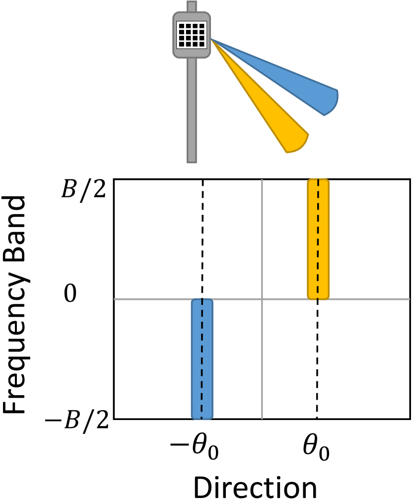
Figure 10: Desired frequency-space beam response for 2 users at directions $-\theta_{0}$ and $\theta_{0}$.

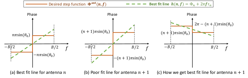
Figure 11: Sketch of proof: We show the phase response for each antenna is a step function with a variable step size that depends on the antenna index, $n$. (a) The objective is to fit a line to this step function in such a way that the error in the line fitting is minimized. (b) we show that as the antenna index increases to say, $n+1$, the step size of the step function also increases linearly with the antenna index. An increase in step-size leads to higher errors in line fitting. (c) We address this issue by reducing the step size by $2\pi$, which will not change the desired phase response but will help to reduce the error.

-A1 Simple two-beam case

Here we derive what set of delays and phases per antenna would give us the beamforming gain pattern with the desired beam-bandwidth and beam direction for the two-beam case. We consider a simple case of two beams with equal beam-bandwidth of $B/2$ each, where $B$ is the total system bandwidth. We assume the two beams are directed along $(-\theta_{0},\theta_{0})$ respectively, as shown in Figure 11. We will later discuss a general case with arbitrary beam-bandwidth and beam directions.

$\blacksquare$ Theorem 1.

(2-beam case) The closed-form expression for the set of delays $\tau_{n}$ and phases $\Phi_{n}$ for each antenna $n$ ($n=0,1,\ldots,N-1$) that would generate a given two-beam response with equal beam-bandwidth $B/2$ and angles $\pm\theta_{0}$ respectively is as follow:

$$\tau_{n}=\left(\frac{3}{2B}n\sin(\theta_{0})+\frac{3}{4B}\right)\;\;\;\text{mod }\frac{3}{2B}$$ (11)

$$\Phi_{n}=\text{round}(n\sin(\theta_{0}))\pi\;\;\;\text{mod }2\pi$$ (12)

We emphasize key takeaways from these expressions before jumping into their proof. Note that the delay values are bounded within a range of $\frac{3}{2B}$ independent of the number of antennas. Within this range, the delay values will monotonically increase or decrease with antenna index $n$, but for large $n$, the delay wraps around with this range factor. This allows for a smaller range of delay values in the DPA hardware independent of the number of antennas.

We now provide proof for the delay and phase expression and throw more insights into the bounded nature of delay and phase values.

Proof for Theorem 1.

(2-beam case) We provide a derivation along with high-level intuition on obtaining a closed-form expression for the delay and phase values. We will first formulate the objective function as an NP-hard problem and then provide an alternate optimization strategy as a set of linear equations that best approximates the solution. We first define the beamforming gain function as a function of frequency $f$ and direction $\theta$ and then look for maximizing this function at the desired frequency-direction pairs. The beamforming gain is given by:

$$G(f,\theta)=\sum_{n=0}^{N-1}e^{j\Phi_{n}+j2\pi f\tau_{n}}e^{-jn\pi\sin(\theta)}$$ (13)

Now, the objective is to maximize the beamforming gain $\left\|G(f,\theta)\right\|^{2}$ at desired beam-bandwidth at given directions $\pm\theta_{0}$ as follows:

$$\begin{split}&\max_{\tau_{n},\Phi_{n}}\quad\left\|G(f,\theta)\right\|^{2}\\ &s.t.\quad\theta=\begin{cases}-\theta_{0}&f\in[\frac{-B}{2},0)\\ \theta_{0}&f\in[0,\frac{B}{2}]\end{cases}\end{split}$$ (14)

Notice that the direction and frequency have a non-linear relationship in the constraints. Specifically, the direction $\theta$ is a non-linear step function of frequency $f$, with a jump at frequency $f=0$. It jumps from the value $-\theta_{0}$ to $+\theta_{0}$ at this frequency. Because of this non-linear dependence of direction with frequency, the underlying optimization problem is NP-hard and cannot be solved optimally. We provide insight into the problem from a different angle and formulate a near-optimal optimization that can be solved to a closed-form expression.

To simplify the above optimization, We define two new functions $h(n,f)$ and $\Phi^{\text{ant}}(n,f)$ below to simplify the non-linear constraint and re-write the optimization problem as follows:

$$\begin{split}\max_{\tau_{n},\Phi_{n}}&\left\|\sum_{n=0}^{N-1}e^{jh(n,f)}e^{-j\Phi^{\text{ant}}(n,f)}\right\|^{2}\\ s.t.\quad&h(n,f)=\Phi_{n}+2\pi f\tau_{n}\\ \text{and}\quad&\Phi^{\text{ant}}(n,f)=\begin{cases}-n\pi\sin(\theta_{0})&f\in[\frac{-B}{2},0]\\ n\pi\sin(\theta_{0})&f\in(0,\frac{B}{2}]\\ \end{cases}\end{split}$$ (15)

where $h(n,f)$ is a function of variable phase $\Phi_{n}$ and delay $\tau_{n}$ at antenna $n$ and the function $\Phi^{\text{ant}}(n,f)$ represents the constraints from the desired frequency-direction response. Let’s see how these functions help us to simplify the optimization problem. Specifically, we apply triangle inequality to find an upper bound on the optimization variable and then maximize this upper bound. Triangle inequality states that the ‘norm-of-sum is upper bounded by sum-of-norms’, which we can apply to our optimization as:

$$\left\|\sum_{n=0}^{N-1}e^{jh(n,f)}e^{-j\Phi^{\text{ant}}(n,f)}\right\|\leq\sum_{n=0}^{N-1}\left\|e^{jh(n,f)}e^{-j\Phi^{\text{ant}}(n,f)}\right\|=N$$ (16)

So, the expression is maximized if each term in the sum is unity, i.e., $e^{jh(n,f)}e^{-j\Phi^{\text{ant}}(n,f)}=1$, or, in other words, the two exponential terms are equal, i.e., $h(n,f)=\Phi^{\text{ant}}(n,f)$ for each antenna and for each frequency. It is impossible to achieve this solution for all frequencies because the two functions $h$ and $\Phi^{\text{ant}}$ vary differently with frequency; $h$ is linear, while $\Phi_{\text{ant}}$ is a step function as shown in Figure 11(a). The only case when the optimal results are possible is when the step size of the step function $\Phi^{\text{ant}}$ is zero, i.e., the two beams align to the same angle. In this case, the step function is reduced to a line, and optimal $h$ can be obtained. However, this case only produces a single beam without any dependence on frequency. A natural question is how we can obtain general frequency-dependent multi-beams. We propose an optimization framework that can help to find a closed-form expression for delays and phases. Our optimization problem is formulated in a way that finds the line $h$ that best fits the given step function $\Phi^{\text{ant}}$. We achieve this by solving the following optimization problem on a per-antenna basis:

$$\begin{split}&\min_{\tau_{n},\Phi_{n}}||h(n,f)-\Phi^{\text{ant}}(n,f)||^{2}\\ \end{split}$$ (17)

We can visualize this optimization in Figure 11(a), where the line $h(n,f)$ is fit over the step function $\Phi^{\text{ant}}(n,f)$. The slope of the best-fit line gives the delay value, and the y-intercept gives the phase value. In this way, we can estimate both delay and phase values by solving for the best-fit line.

However, as antenna index $n$ increases, the error in line fitting also increases due to the linear increase in the step size with $n$, as shown in Figure 11(b). This could lead to high error for large antenna arrays and limit our solution to scale with antennas. We have an innovative and simple solution to address this issue. To address this issue, we utilize the concept of wrapping the phase of a signal by $2\pi$, i.e., adding an integer multiple of $2\pi$ to the phase does not change the signal. We use this idea to strategically add a phase of multiple of $2\pi$ to a specific set of frequencies in order to minimize the error in line fitting as shown in Figure 11(c). With this insight, we redefine the step function $\Phi^{\text{ant}}$ as:

$$\Phi^{\text{ant}}(n,f)=\begin{cases}k2\pi-n\pi\sin(\theta_{0})&f\in[\frac{-B}{2},0]\\ n\pi\sin(\theta_{0})&f\in(0,\frac{B}{2}]\\ \end{cases}$$ (18)

where $k$ is a constant integer. A natural question is how do we estimate this integer to minimize the error in line fitting? Our solution is a two-step process: we solve for the delays and phases as a function of $k$ and then find the optimal value of $k$ to minimize the error. We now describe how we solve for the best-fit line to estimate the per-antenna delay and phase values.

To solve for per-antenna delays and phases, we form a system of linear equations. We first discretize the frequency as $f=m\Delta f$ for $m\in[-M/2,M/2]$, where the bandwidth is $B=(M+1)\Delta f$. Note that there are $M$ frequency bins that can be a large number, i.e., $M\rightarrow\infty$ for creating a continuous frequency axis. We then formulate a set of linear equations for each frequency term to solve for the variable delay $\tau_{n}$ and phase $\Phi_{n}$ for each antenna $n$. Specifically, we have the following linear equations:

$$\Phi_{n}+2\pi m\Delta f\tau_{n}=\Phi^{\text{ant}}(n,m\Delta f)\;\forall m\in[-M/2,M/2]$$ (19)

We re-write the equations in a matrix form as follows:

$$Ax=b$$ (20)

where $x$ is a $2\times 1$ vector of variable phase and delay given by:

$$x=\begin{bmatrix}\Phi_{n}\\ 2\pi\Delta f\tau_{n}\end{bmatrix}$$ (21)

and the matrix $A$ and vector $b$ are constants given by:

$$A=\begin{bmatrix}1&\frac{-M}{2}\\ 1&\frac{-M}{2}+1\\ \vdots&\vdots\\ 1&\frac{M}{2}\end{bmatrix}$$ (22)

$$b=\begin{bmatrix}\underbrace{k2\pi-\phi\;\ldots\;k2\pi-\phi}_{M/2}\;\underbrace{\phi\ldots\phi}_{M/2+1}\end{bmatrix}^{T}$$ (23)

where $\phi=n\pi\sin(\theta_{0})$ is introduced for simplicity. Specifically, we add $k2\pi$ to the first half of the frequency subcarriers, and this is reflected in the value of $b$.

The solution can be obtained by solving a system of linear equations as follow:

$$x=(A^{T}A)^{-1}A^{T}b$$ (24)

We first solve for $(A^{T}A)^{-1}$ and $A^{T}b$ separately and then multiply them together to get $x$:

$$\begin{split}A^{T}A&=\begin{bmatrix}1&1&\ldots&1\\ \frac{-M}{2}&\frac{-M}{2}+1&\ldots&\frac{M}{2}\end{bmatrix}\begin{bmatrix}1&\frac{-M}{2}\\ 1&\frac{-M}{2}+1\\ \vdots&\vdots\\ 1&\frac{M}{2}\end{bmatrix}\\ &=\begin{bmatrix}M+1&0\\ 0&2\sum_{0}^{\frac{M}{2}}k^{2}\end{bmatrix}=\begin{bmatrix}M+1&0\\ 0&\frac{M(M+1)(M+2)}{12}\end{bmatrix}\end{split}$$ (25)

Taking the inverse of the above 2x2 matrix, we get

$$(A^{T}A)^{-1}=\begin{bmatrix}\frac{1}{M+1}&0\\ 0&\frac{12}{M(M+1)(M+2)}\end{bmatrix}$$ (26)

This solves for $A^{T}A$. Next, we obtain $A^{T}b$ as:

$$\begin{split}A^{T}b&=\begin{bmatrix}1&1&\ldots&1\\ \frac{-M}{2}&\frac{-M}{2}+1&\ldots&\frac{M}{2}\end{bmatrix}\\ &\times\begin{bmatrix}\underbrace{k2\pi-\phi\;\ldots\;k2\pi-\phi}_{M/2}\;\underbrace{\phi\ldots\phi}_{M/2+1}\end{bmatrix}^{T}\\ &=\begin{bmatrix}\phi+kM\pi\\ (2\phi-k2\pi)\sum_{1}^{M/2}m\end{bmatrix}\\ &=\begin{bmatrix}\phi+kM\pi\\ (\phi-k\pi)\frac{M(M+2)}{4}\end{bmatrix}\end{split}$$ (27)

This solves for $A^{T}b$. We now obtain the solution for unknown $x$ as follows:

$$\begin{split}x&=(A^{T}A)^{-1}A^{T}b\\ &=\begin{bmatrix}\frac{1}{M+1}&0\\ 0&\frac{12}{M(M+1)(M+2)}\end{bmatrix}A^{T}b\\ &=\begin{bmatrix}A^{T}b[1]\frac{1}{M+1}\\ A^{T}b[2]\frac{12}{(M(M+1)(M+2))}\end{bmatrix}\end{split}$$ (28)

Finally, using the definition of $x$ from (21), we get the solution for the per antenna phase and delay. The phase is given by $x[1]$ and delay is given by x[2] as follows:

$$\begin{split}\Phi_{n}&=\lim_{M\rightarrow\infty}x[1]=\lim_{M\rightarrow\infty}A^{T}b[1]\frac{1}{M+1}\\ &=\lim_{M\rightarrow\infty}\frac{\phi+kM\pi}{M+1}\\ &=k\pi\end{split}$$ (29)

where the approximation is taken for a large number of frequency bins, i.e., $M\rightarrow\infty$. Similarly, we get the expression for the delay:

$$\begin{split}\tau^{\prime}_{n}&=\frac{x[2]}{2\pi\Delta f}=A^{T}b[2]\frac{12}{M(M+1)(M+2)}\frac{1}{2\pi\Delta f}\\ &=(\phi-k\pi)\frac{M(M+2)}{4}\frac{12}{M(M+1)(M+2)}\frac{1}{2\pi\Delta f}\\ &=\frac{3(\phi-k\pi)}{2\pi\Delta f(M+1)}\\ &=\frac{3(n\sin(\theta_{0})}{2B}-\frac{3k}{2B}\\ &=\frac{3}{2B}(n\sin(\theta_{0})-k)\end{split}$$ (30)

This gives a closed-form expression of delay. Note that the expression for delay and phase both depend on the unknown constant integer $k$. So, how do we solve for $k$ to obtain a generalized formula for delay and phases? Out of many possible solutions, because of the presence of a random integer $k$, we need to choose the value of $k$ that minimizes the error in line fitting. To solve for $k$, we make an observation that the step size of the step function is part of the exponential and therefore is bounded by $2\pi$. Let’s find the condition when the step size is bounded between $-\pi$ and $\pi$ as follows:

$$\begin{split}&-\pi<\phi-(-\phi+k2\pi)\leq\pi\\ \Rightarrow\;\;&\pi<2\phi-k2\pi\leq\pi\\ \Rightarrow\;\;&\pi<2n\pi\sin(\theta_{0})-k2\pi\leq\pi\\ \Rightarrow\;\;&\frac{1}{2}<n\sin(\theta_{0})-k\leq\frac{1}{2}\\ \Rightarrow\;\;&\sin(\theta_{0})-\frac{1}{2}<k\leq\sin(\theta_{0})+\frac{1}{2}\\ \Rightarrow\;\;&k=\text{round}(n\sin(\theta_{0}))\\ \end{split}$$ (31)

Since $k$ is an integer, the only possible value of $k$ is given by $\text{round}(n\sin(\theta_{0}))$. This gives us a unique solution for the integer constant $k$. Putting the in the expression of phase and delay, we get the required phase:

$$\Phi_{n}=\text{round}(n\sin(\theta_{0}))\pi$$ (32)

Similarly, we obtain the final expression of delay as:

$$\begin{split}\tau^{\prime}_{n}&=\frac{3}{2B}(n\sin(\theta_{0})-\text{round}(n\sin(\theta_{0})))\end{split}$$ (33)

We notice the above expression of delay varies in the range of $\frac{-3}{4B}$ to $\frac{3}{4B}$, resulting in a total range of $\frac{3}{2B}$. Since negative delays are not possible to generate in a causal system, we can add a constant delay to all antennas to make delays positive. The minimum constant delay factor that we can add without compromising on the performance is $\frac{3}{4B}$. After adding this factor and simplifying the delay expression, we get the following:

$$\begin{split}\tau_{n}&=\tau^{\prime}_{n}+\frac{3}{4B}\\ &=\frac{3}{2B}(n\sin(\theta_{0})-\text{round}(n\sin(\theta_{0})))+\frac{3}{4B}\\ &=\left(\frac{3}{2B}n\sin(\theta_{0})+\frac{3}{4B}\right)\;\;\;\text{mod }\frac{3}{2B}\end{split}$$ (34)

where the last step is a simplification of the round function into a modulo function for ease of understanding and emphasizing that the range of values of delays is independent of the number of antennas. The delay range is $\frac{3}{2B}$ for two beam case which depends inverse This is how we estimate the final expression of optimal phase $\Phi_{n}$ and delay $\tau_{n}$ in (12) and (11), respectively.

$\Box$

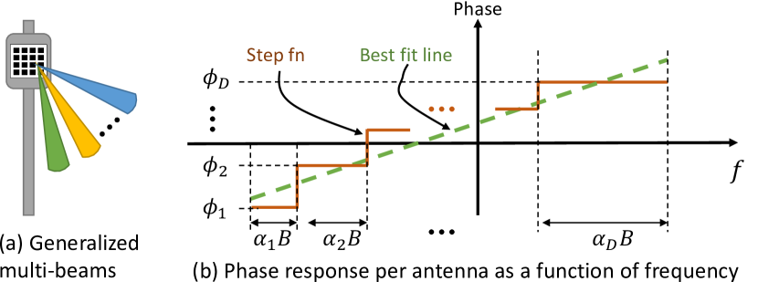
Figure 12: Generalized setting for multi-beams with an arbitrary number of beams $D$, beam angles, and beam-bandwidths. The beam angles contributes to $\phi_{d}$, and the beam-bandwidth is defined as $\alpha_{d}B$ for system bandwidth $B$ and fraction $\alpha_{d}<1$ for beam index $d\leq D$.

-A2 Generalization to an arbitrary number of beams, beam directions, and beam-bandwidth

We now generalize the beamforming response to an arbitrary number of beams with arbitrary beam directions and arbitrary beam-bandwidths as shown in Fig. 12.

$\blacksquare$ Theorem 2.

(Generalized case): Let there are $D$ beam directions with beam angles $\theta_{d}$ and beam-bandwidth $\alpha_{d}B$ for $\sum_{d}\alpha_{d}=1$. We define $\phi_{d}=n\pi\sin(\theta_{d})$ for simplicity. The per-antenna phases and delays in realizing such a generalized beamforming response is given by:

$$\Phi_{n}=\sum_{d=1}^{D}\alpha_{d}(\phi_{d}+2k_{d}\pi)$$ (35)

$$\tau_{n}=\sum_{d=1}^{D}\frac{3}{\pi B}(\phi_{d}+2\pi k_{d})\alpha_{d}(\sum_{\ell=1}^{d}2\alpha_{\ell}-\alpha_{d}-1)$$ (36)

where,

$$\phi_{d}=n\pi\sin(\theta_{d})$$ (37)

and the constant integer $k_{d}$ for beam $d$ and antenna $n$ is:

$$k_{d}=\begin{cases}&0\quad d=1\\ &k_{d-1}\!+\!\text{round}(\frac{n\sin(\theta_{d-1})-n\sin(\theta_{d})}{2})\;\;d\geq 2\end{cases}$$ (38)

Before we provide a derivation for the generalized delay and phase expression, we first verify the expression for the two-beam case by putting $D=2$ in the above expression. We would obtain a generic expression with arbitrary beam-bandwidth and arbitrary beam directions and then simplify it to the case of equal beam-bandwidth and symmetric direction similar to the previous analysis.

$\blacksquare$ Corollary 1.

(Generalized two-beam case) For two beams with beam directions $\theta_{1}$ and $\theta_{2}$ and the beam-bandwidths $\alpha B$ and $(1-\alpha)B$ respectively, such that the bandwidth fraction $0\leq\alpha\leq 1$, the corresponding delays and phases that generate this two-beam response is given by:

$$\Phi_{n}=\alpha\phi_{1}+(1-\alpha)(\phi_{2}+2k_{2}\pi)$$ (39)

$$\tau_{n}=\frac{3}{\pi B}[(-\phi_{1}+\phi_{2}+2\pi k_{2})\alpha(1-\alpha)]$$ (40)

for $\phi_{1}=n\pi\sin(\theta_{1})$ and $\phi_{2}=n\pi\sin(\theta_{2})$, and the constant integer $k_{2}$ defined as

$$k_{2}=\text{round}(\frac{n\sin(\theta_{1})-n\sin(\theta_{2})}{2})$$ (41)

Proof of Corollary 1.

We prove the corollary for the two-beam case by putting the number of beams $D=2$ in the generalized expressions and further simplify them with $\alpha_{1}=\alpha$ and $\alpha_{2}=1-\alpha$. Also, note that $k_{1}=0$, by definition. We now simplify the phase as follows:

$$\begin{split}\Phi_{n}&=\alpha_{1}(\phi_{1}+2k_{1}\pi)+\alpha_{2}(\phi_{2}+2k_{2}\pi)\\ &=\alpha\phi_{1}+(1-\alpha)(\phi_{2}+2k_{2}\pi)\\ \end{split}$$ (42)

and delay

$$\begin{split}\tau_{n}&=\frac{3}{\pi B}[(\phi_{1}+2\pi k_{1})\alpha_{1}(\alpha_{1}-1)\\ &\quad+(\phi_{2}+2\pi k_{2})\alpha_{2}(2\alpha_{1}+\alpha_{2}-1)]\\ &=\frac{3}{\pi B}[(\phi_{1})\alpha(\alpha-1)+(\phi_{2}+2\pi k_{2})(1-\alpha)(\alpha)]\\ &=\frac{3}{\pi B}[(-\phi_{1}+\phi_{2}+2\pi k_{2})\alpha(1-\alpha)]\\ \end{split}$$ (43)

This proves the corollary. $\Box$

We will now verify the delays and phases for the special case of equal beam-bandwidth, i.e., $\alpha=1/2$ and symmetric angles, i.e., $\phi_{1}=-n\pi\sin(\theta_{0})$ and $\phi_{2}=n\pi\sin(\theta_{0})$. In this case, we get $k_{2}=-\text{round}(n\sin(\theta_{0}))$ and a simplified phase as:

$$\begin{split}\Phi_{n}&=\alpha\phi_{1}+(1-\alpha)(\phi_{2}+2k_{2}\pi)\\ &=\phi_{1}/2+\phi_{2}/2+k_{2}\pi\\ &=k_{2}\pi\\ &=-\text{round}(n\sin(\theta_{0}))\pi\\ &=\text{round}(n\sin(\theta_{0}))\pi\end{split}$$ (44)

which is an integer multiple of $\pi$, where the integer multiple is given by $\text{round}(n\sin(\theta_{0}))$. This expression is the same as what we derived earlier in (32). We now get delay expression as:

$$\begin{split}\tau_{n}&=\frac{3}{\pi B}[(-\phi_{1}+\phi_{2}+2\pi k_{2})\alpha(1-\alpha)]\\ &=\frac{3}{\pi B}[(n\pi\sin(\theta_{0})+n\pi\sin(\theta_{0})+2\pi k_{2})\alpha(1-\alpha)]\\ &=\frac{3}{B}[(2n\sin(\theta_{0})+2k_{2})\alpha(1-\alpha)]\\ &=\frac{3}{2B}(n\sin(\theta_{0})+k_{2})\\ &=\frac{3}{2B}(n\sin(\theta_{0})-\text{round}(n\sin(\theta_{0})))\\ \end{split}$$ (45)

This delay expression is the same as what we have derived earlier for the simple 2-beam case in (33). This validates the generalized multi-beam expressions for two beams. We now prove the generalized expression for an arbitrary number of beams, beam directions, and beam-bandwidths.

Proof of Theorem 2.

(Generalized case) We follow the same formulation as before as a set of linear equations with a new set of constraints for the generalized case. We notice that the constant matrix $A$ doesn’t change for the generalized case, and only the constant vector $b$ is modified. We would solve for delays and phases similar to the simple 2-beam case using pseudo-inverse (Recall $x=(A^{T}A)^{-1}A^{T}b$).

We start with a generic expression for vector $b$ as:

$$b=\begin{bmatrix}\underbrace{\phi_{1}+k_{1}2\pi\ldots,}_{\alpha_{1}M}\underbrace{\;\ldots\;}_{\ldots}\underbrace{,\ldots\phi_{D}+k_{D}2\pi}_{(\alpha_{D})M}\end{bmatrix}^{T}$$ (46)

Therefore, solution for $A^{T}b$ is now:

$$\begin{split}A^{T}b&=\begin{bmatrix}1&1&\ldots&1\\ \frac{-M}{2}&\frac{-M}{2}+1&\ldots&\frac{M}{2}\end{bmatrix}b\end{split}$$ (47)

We first solve for phase. Since the matrix $A$ is unchanged, we directly apply $(A^{T}A)^{-1}$ from the two-beam case (29) and solve for the per-antenna phase as follows:

$$\begin{split}\Phi_{n}&=\lim_{M\rightarrow\infty}A^{T}b[1]\frac{1}{M+1}\\ &=\lim_{M\rightarrow\infty}\frac{\sum_{d=1}^{D}\alpha_{d}M(\phi_{d}+2k_{d}\pi)}{M+1}\\ &=\sum_{d=1}^{D}\alpha_{d}(\phi_{d}+2k_{d}\pi)\end{split}$$ (48)

This proves the expression of phase. We now solve for the delay in a similar way as we solved for the two-beam case in (30) as follows:

$$\begin{split}\tau_{n}&=\lim_{M\rightarrow\infty}A^{T}b[2]\frac{12}{M(M+1)(M+2)}\frac{1}{2\pi\Delta f}\\ &=\lim_{M\rightarrow\infty}A^{T}b[2]\frac{12}{M(M+2)}\frac{1}{2\pi B}\\ &=\lim_{M\rightarrow\infty}\bigl{[}(\phi_{1}+k_{1}2\pi)(-\sum_{m=0}^{M/2}m+\sum_{m=0}^{\alpha_{1}M-M/2}m)\\ &\quad\quad+(\phi_{2}+k_{2}2\pi)(-\sum_{m=0}^{\alpha_{1}M-M/2}m+\sum_{m=0}^{(\alpha_{1}+\alpha_{2})M-M/2}m)\\ &\quad\cdots+(\phi_{D}+k_{D}2\pi)(\sum_{m=0}^{\sum_{\ell=1}^{D}\alpha_{\ell}M-M/2}\!\!\!\!\!m-\sum_{m=0}^{\sum_{\ell=1}^{D-1}\alpha_{\ell}M-M/2}\!\!\!\!\!m)\bigr{]}\\ &\quad\quad\times\frac{12}{M(M+2)}\frac{1}{2\pi B}\\ \end{split}$$ (49)

where we put the expression for $B=(M+1)\Delta f$ for simplification. Still, the above expression is complex and messy, which we intend to write in a simplified closed-form solution. Our idea to simplify the above expression is that since there is a $M^{2}$ term in the denominator, we only collect the $M^{2}$ terms from the numerator and ignore other constant or linear terms. This is because we are interested in the case when the number of frequency bins is very high, i.e., $\lim_{M\rightarrow\infty}$. This leads to a simplified expression as follows:

$$\begin{split}\tau_{n}&=\frac{3}{\pi B}\bigl{[}(\phi_{1}+k_{1}2\pi)(-(1/2)^{2}+(\alpha_{1}-1/2)^{2})\\ &\quad\quad+(\phi_{2}+k_{2}2\pi)(-(\alpha_{1}-1/2)^{2}+(\alpha_{1}+\alpha_{2}-1/2)^{2})\\ &\quad\quad\cdots(\phi_{D}+k_{D}2\pi)((\sum_{\ell=1}^{D}\alpha_{\ell}-1/2)^{2}-(\sum_{\ell=1}^{D-1}\alpha_{\ell}-1/2)^{2})\bigr{]}\\ &=\frac{3}{\pi B}\bigl{[}(\phi_{1}+k_{1}2\pi)(\alpha_{1}(\alpha_{1}-1))\\ &\quad\quad+(\phi_{2}+k_{2}2\pi)(\alpha_{2}(2\alpha_{1}+\alpha_{2}-1))\\ &\quad\quad\cdots(\phi_{D}+k_{D}2\pi)(\alpha_{D}(\sum_{\ell=1}^{D-1}2\alpha_{\ell}+\alpha_{D}-1))\bigr{]}\\ \end{split}$$ (50)

This proves the generalized expression for phases and delays in (35) and (36), respectively, for an arbitrary number of beams, beam directions, and beam-bandwidth. $\Box$

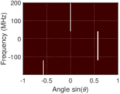
(a) Desired F-S response

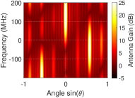
(b) FSDA F-S response

(c) Math F-S response

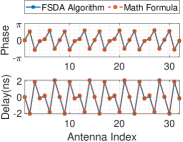
(d) Phases and Delays

Figure 13: Generalized 3-beam case: Comparing the Frequency-Space (F-S) beamforming response of FSDA algorithm and Maths.

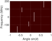
(a) Desired F-S response

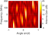
(b) FSDA F-S response

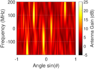
(c) Math F-S response

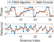
(d) Phases and Delays

Figure 14: Generalized 5-beam case: Comparing the Frequency-Space (F-S) beamforming response of FSDA algorithm and Maths.

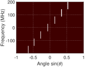
(a) Desired F-S response

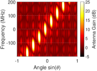
(b) FSDA F-S response

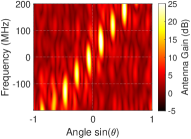
(c) Math F-S response

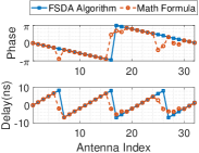
(d) Phases and Delays

Figure 15: Uniform 7-beam case: Comparing the Frequency-Space (F-S) beamforming response of FSDA algorithm and Maths.

We now discuss insights into how we obtain the expression for the unknown integer constant $k_{d}$ to bind the error in line fitting. Recall in the two-beam system, we have seen that by strategically adding an integer multiple of $2\pi$ to the phase of one beam, we can reduce the error in line fitting without changing the actual value of the phase. This is due to the concept of phase wrapping, where adding $2\pi$ to a phase value results in the same point on the complex plane.

To generalize this insight for an arbitrary number of beams, we need to ensure that the phase difference between any two consecutive beams is less than $\pi$. Because if the phase difference goes more than $\pi$, then we can always add $2\pi$ to the phase of one of the two consecutive beams to make the phase difference less than $\pi$. By doing this, we can ensure that the step size doesn’t grow high for a large antenna index, thus minimizing the error in line fitting. To obtain the expression for the integer constant $k_{d}$ for each beam $d$, we start by fixing the phase of the first beam and then adjust the phase of the second beam with respect to the first beam and follow this process to all consecutive antennas: adjust the phase of $d$th beam with respect to the $d-1$th beam. This ensures that no two consecutive beams have a phase difference greater than $\pi$. This results in the final expression for $k_{d}$ in (38), which expresses the integer constant multiple of $2\pi$ that is added to the phase of each beam to achieve the desired bound on the phase difference. This bound on phase difference leads to a bound on the error in line fitting, resulting in an accurate line fitting for generalized multi-beam systems.

-B Evaluation of Mathematical Multi-beam patterns

Here we provide an extensive evaluation for mmFlexible under different scenarios. We compare the beamforming patterns that are produced by Mathematical expression vs FSDA algorithm. We also show the impact of delay and phase quantization to show the practical performance of mmFlexible.

$\blacksquare$ Comparison of Maths expression vs. FSDA algorithm: We present several examples of joint frequency-space beamforming using the DPA architecture. We utilize a 32-element linear antenna array with programmable phase and delay elements per antenna in various scenarios, including three-beam, five-beam, and seven-beam configurations as shown in Figure 13, 14, and  15 respectively. In, Figure 13(a), we show a desired frequency-space (F-S) image that illustrates high intensity at the desired frequency-direction pairs, where we want high array gain. We then show two F-S images that were obtained through DPA after programming them using the FSDA algorithm and a mathematical expression in Figure 13(b) and (c), respectively. Additionally, we present the set of delays and phase values obtained from the FSDA algorithm and mathematical expression at each of the 32 antennas in Figure 13(d).

1. DPA can reasonably achieve the desired multi-beam patterns with an arbitrary number of beams, beam directions and beam bandwidths. We observe that the antenna gain is high in the desired frequency-direction pairs and low elsewhere, as expected. This verifies that the linear approximation of the non-linear per-antenna phase profile is fairly accurate. However, at the edges of each beam, there may be a gradual transition instead of a sharp one. This can be seen at the boundary of the frequency band supported by each beam, but it only occurs along the frequency band and not in the angular domain. The beams remain sharp in the intended directions and do not spread to other unwanted angular directions.

2. We compared two F-S images created by the FSDA algorithm and a mathematical expression and found that the patterns produced by the FSDA algorithm are more precise and sharp. For example, the FSDA can create small beam bandwidths, while the mathematical patterns have wider bandwidths. The difference in the final F-S images produced by each method can be attributed to small variations in the set of delays and phases obtained by the FSDA and the mathematical approach, which we observed in 15(d). The difference in the FSDA and mathematical approach is caused by the heuristic method of obtaining the integer constant $k_{d}$ used to scale the phase profile of beam $d$, which reduces the error in line fitting. The mathematical approach is more conservative, as it prefers solutions with shorter delays over longer delays obtained by the FSDA for the same desired F-S response. However, the difference in the patterns obtained from both approaches is small, and both methods demonstrate the ability to create frequency-dependent multi-beam patterns.

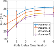
(a) Delay Quantization

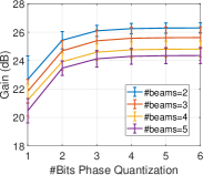
(b) Phase Quantization

Figure 16: Effect of delay and phase quantization in overall array gain of 16 antennae DPA.

$\blacksquare$ Effect of phase and delay quantization: We are now investigating the effect of quantization on the performance of the mmFlexible system. The DPA antenna array hardware must be designed with a certain level of quantization in the values of delays and phases. The more quantization bits used, the better the array’s performance will be, but this also increases the complexity of the hardware design. This creates a trade-off between the number of quantization bits and the gain performance of the array. We have shown in Figure 16 that the array gain improves as the number of quantization bits is increased from 1 to 6 for both delay and phase quantization. However, the improvement in the array gain becomes small for higher numbers of bits and reaches a saturation point. Specifically, the array gain improves by less than 1 dB when the quantization is increased from 3 bits. Therefore, practical mmFlexible hardware can be designed with a minimum of 3-bit quantization in phase/delay while maintaining high performance.

-C Conclusion for Appendix

In this appendix, we presented a detailed mathematical analysis of the delay-phased array (DPA) and derived a closed-form mathematical expression for delay and phase values. We proposed an innovative approach for representing the per-antenna phase profile as a function of frequency and demonstrated that an ideal phase profile is in the form of a step function with the number of steps equal to the number of beams and the step size and width dependent on the beam directions and beam-bandwidth, respectively. We emphasized the challenge of realizing this non-linear phase profile using analog hardware, as it does not provide precise control over each frequency component in the signal. To overcome this limitation, we developed an approximate near-optimal method that utilizes a line-fitting method to derive the best-fit line for the given step function. The slope of the best-fit line gives the delay estimate, while the y-intercept gives the phase estimate. This method enables the derivation of delay and phase values in closed form and provides a deeper understanding of their behavior.

In particular, we showed that the delay values are always bounded within a small range that is independent of the number of antennas, similar to how the phase is bounded by $2\pi$. This allows for the creation of practical hardware with shorter delay lines, in contrast to traditional Rainbow-link architectures [1], which require long delay lines. We also demonstrated the application of DPA in flexible directional frequency multiplexing, where frequency-dependent multi-beam patterns can be used to extend mmWave connectivity to IoT and URLLC applications by concurrently serving many devices with a small chunk of bandwidth while maintaining a directional link with all devices. Additionally, it can aid in concurrent control and communication by creating multiple pencil beams, with one dedicated beam carrying beam scan control messages and the other beams carrying communication data toward the direction of an active user.

References

- [1] R. Li, H. Yan, and D. Cabric, “Rainbow-link: Beam-alignment-free and grant-free mmw multiple access using true-time-delay array,” IEEE Journal on Selected Areas in Communications, 2022.
- [2] H. Yan, V. Boljanovic, and D. Cabric, “Wideband millimeter-wave beam training with true-time-delay array architecture,” in 2019 53rd Asilomar Conference on Signals, Systems, and Computers. IEEE, 2019, pp. 1447–1452.
- [3] V. Boljanovic, H. Yan, C.-C. Lin, S. Mohapatra, D. Heo, S. Gupta, and D. Cabric, “Fast beam training with true-time-delay arrays in wideband millimeter-wave systems,” IEEE Transactions on Circuits and Systems I: Regular Papers, vol. 68, no. 4, pp. 1727–1739, 2021.
- [4] Y. Ghasempour, R. Shrestha, A. Charous, E. Knightly, and D. M. Mittleman, “Single-shot link discovery for terahertz wireless networks,” Nature communications, vol. 11, no. 1, pp. 1–6, 2020.
- [5] E. Ghaderi, A. S. Ramani, A. A. Rahimi, D. Heo, S. Shekhar, and S. Gupta, “An integrated discrete-time delay-compensating technique for large-array beamformers,” IEEE Transactions on Circuits and Systems I: Regular Papers, vol. 66, no. 9, pp. 3296–3306, 2019.
- [6] V. Boljanovic, H. Yan, C.-C. Lin, S. Mohapatra, D. Heo, S. Gupta, and D. Cabric, “True-time-delay arrays for fast beam training in wideband millimeter-wave systems,” arXiv preprint arXiv:2007.08713, 2020.
- [7] A. R. Qualcomm, “Augmented and virtual reality: the first wave of 5g killer apps,” https://www.qualcomm.com/content/dam/qcomm-martech/dm-assets/documents/cr-qcom-140.pdf, 2017.
- [8] G. Pocovi, H. Shariatmadari, G. Berardinelli, K. Pedersen, J. Steiner, and Z. Li, “Achieving ultra-reliable low-latency communications: Challenges and envisioned system enhancements,” IEEE Network, vol. 32, no. 2, pp. 8–15, 2018.
- [9] “Speech and multimedia Transmission Quality (STQ); QoS parameters and test scenarios for assessing network capabilities in 5G performance measurements,” 3rd Generation Partnership Project (3GPP), TR ETSI TR 103 702 V1.1.1 , 2020-11. [Online]. Available: http://www.etsi.org/deliver/etsi˙tr/138900˙138999/138901/14.00.00˙60/tr˙138901v140000p.pdf
- [10] S. Mangiante, G. Klas, A. Navon, Z. GuanHua, J. Ran, and M. D. Silva, “Vr is on the edge: How to deliver 360 videos in mobile networks,” in Proceedings of the Workshop on Virtual Reality and Augmented Reality Network, 2017, pp. 30–35.
- [11] J. Benesty, I. Cohen, and J. Chen, Array Processing. Springer, 2019.
- [12] A. Nagulu, A. Gaonkar, S. Ahasan, S. Garikapati, T. Chen, G. Zussman, and H. Krishnaswamy, “A full-duplex receiver with true-time-delay cancelers based on switched-capacitor-networks operating beyond the delay–bandwidth limit,” IEEE Journal of Solid-State Circuits, vol. 56, no. 5, pp. 1398–1411, 2021.
- [13] E. Ghaderi and S. Gupta, “A four-element 500-mhz 40-mw 6-bit adc-enabled time-domain spatial signal processor,” IEEE Journal of Solid-State Circuits, vol. 56, no. 6, pp. 1784–1794, 2020.
- [14] I. K. Jain, R. Subbaraman, T. H. Sadarahalli, X. Shao, H.-W. Lin, and D. Bharadia, “mmobile: Building a mmwave testbed to evaluate and address mobility effects,” in Proceedings of the 4th ACM Workshop on Millimeter-Wave Networks and Sensing Systems, 2020, pp. 1–6.
- [15] D. Caudill, J. Chuang, S. Y. Jun, C. Gentile, and N. Golmie, “Real-time mmwave channel sounding through switched beamforming with 3-d dual-polarized phased-array antennas,” IEEE Transactions on Microwave Theory and Techniques, vol. 69, no. 11, pp. 5021–5032, 2021.
- [16] J. Palacios, “Adaptive Codebook Optimization for Beam Training on Off-the-Shelf IEEE 802.11ad Devices,” in Proceedings of the 24rd Annual International Conference on Mobile Computing and Networking. ACM, 2018.
- [17] M. Giordani, M. Polese, A. Roy, D. Castor, and M. Zorzi, “A tutorial on beam management for 3GPP NR at mmWave frequencies,” IEEE Communications Surveys & Tutorials, vol. 21, no. 1, pp. 173–196, 2018.
- [18] alvarovalcarce, “Nokia wireless suite - github reference,” https://github.com/nokia/wireless-suite (2020/11/12).
- [19] I. K. Jain, R. Kumar, and S. S. Panwar, “The impact of mobile blockers on millimeter wave cellular systems,” IEEE Journal on Selected Areas in Communications, vol. 37, no. 4, pp. 854–868, 2019.
- [20] “5G; Study on channel model for frequencies from 0.5 to 100 GHz,” 3rd Generation Partnership Project (3GPP), TR 138 901 V14.0.0, 2017-05. [Online]. Available: http://www.etsi.org/deliver/etsi˙tr/138900˙138999/138901/14.00.00˙60/tr˙138901v140000p.pdf
- [21] I. K. Jain, R. Subbaraman, and D. Bharadia, “Two beams are better than one: towards reliable and high throughput mmwave links,” in Proceedings of the 2021 ACM SIGCOMM 2021 Conference, 2021, pp. 488–502.
- [22] I. Aykin, B. Akgun, and M. Krunz, “Multi-beam transmissions for blockage resilience and reliability in millimeter-wave systems,” IEEE Journal on Selected Areas in Communications, vol. 37, no. 12, pp. 2772–2785, 2019.
- [23] J. A. Zhang, X. Huang, Y. J. Guo, J. Yuan, and R. W. Heath, “Multibeam for joint communication and radar sensing using steerable analog antenna arrays,” IEEE Transactions on Vehicular Technology, vol. 68, no. 1, pp. 671–685, 2018.
- [24] H. Hassanieh, O. Abari, M. Rodriguez, M. Abdelghany, D. Katabi, and P. Indyk, “Fast millimeter wave beam alignment,” in Proceedings of the 2018 Conference of the ACM Special Interest Group on Data Communication. ACM, 2018, pp. 432–445.
- [25] D. Zhu, J. Choi, Q. Cheng, W. Xiao, and R. W. Heath, “High-resolution angle tracking for mobile wideband millimeter-wave systems with antenna array calibration,” IEEE Transactions on Wireless Communications, vol. 17, no. 11, pp. 7173–7189, 2018.
- [26] R. Rotman, M. Tur, and L. Yaron, “True time delay in phased arrays,” Proceedings of the IEEE, vol. 104, no. 3, pp. 504–518, 2016.
- [27] S. K. Garakoui, E. A. Klumperink, B. Nauta, and F. E. van Vliet, “Compact cascadable gm-c all-pass true time delay cell with reduced delay variation over frequency,” IEEE journal of solid-state circuits, vol. 50, no. 3, pp. 693–703, 2015.
- [28] A. Wadaskar, V. Boljanovic, H. Yan, and D. Cabric, “3D Rainbow Beam Design for Fast Beam Training with True-Time-Delay Arrays in Wideband Millimeter-Wave Systems,” in 2021 55th Asilomar Conference on Signals, Systems, and Computers. IEEE, 2021, pp. 85–92.
- [29] V. Boljanovic and D. Cabric, “Compressive estimation of wideband mmw channel using analog true-time-delay array,” in 2021 IEEE Workshop on Signal Processing Systems (SiPS). IEEE, 2021, pp. 170–175.
- [30] J. Tan and L. Dai, “Wideband beam tracking in thz massive mimo systems,” IEEE Journal on Selected Areas in Communications, vol. 39, no. 6, pp. 1693–1710, 2021.
- [31] ——, “Delay-phase precoding for thz massive mimo with beam split,” in 2019 IEEE Global Communications Conference (GLOBECOM). IEEE, 2019, pp. 1–6.
- [32] V. V. Ratnam, J. Mo, A. Alammouri, B. L. Ng, J. Zhang, and A. F. Molisch, “Joint phase-time arrays: A paradigm for frequency-dependent analog beamforming in 6g,” IEEE Access, vol. 10, pp. 73 364–73 377, 2022.
- [33] R. Garg, G. Sharma, A. Binaie, S. Jain, S. Ahasan, A. Dascurcu, H. Krishnaswamy, and A. S. Natarajan, “A 28-ghz beam-space mimo rx with spatial filtering and frequency-division multiplexing-based single-wire if interface,” IEEE Journal of Solid-State Circuits, 2020.
- [34] M.-K. Cho, I. Song, and J. D. Cressler, “A true time delay-based sige bi-directional t/r chipset for large-scale wideband timed array antennas,” in 2018 IEEE Radio Frequency Integrated Circuits Symposium (RFIC). IEEE, 2018, pp. 272–275.
- [35] F. Hu and K. Mouthaan, “A 1–20 ghz 400 ps true-time delay with small delay error in 0.13 m cmos for broadband phased array antennas,” in 2015 IEEE MTT-S International Microwave Symposium. IEEE, 2015, pp. 1–3.
- [36] L.-H. Shen and K.-T. Feng, “Mobility-aware subband and beam resource allocation schemes for millimeter wave wireless networks,” IEEE Transactions on Vehicular Technology, vol. 69, no. 10, pp. 11 893–11 908, 2020.
- [37] W. Zhang, Y. Wei, S. Wu, W. Meng, and W. Xiang, “Joint beam and resource allocation in 5g mmwave small cell systems,” IEEE Transactions on Vehicular Technology, vol. 68, no. 10, pp. 10 272–10 277, 2019.