Divide and Conquer Dynamic Programming: An Almost Linear Time Change Point Detection Methodology in High Dimensions

Abstract

We develop a novel, general and computationally efficient framework, called Divide and Conquer Dynamic Programming (DCDP), for localizing change points in time series data with high-dimensional features. DCDP deploys a class of greedy algorithms that are applicable to a broad variety of high-dimensional statistical models and can enjoy almost linear computational complexity. We investigate the performance of DCDP in three commonly studied change point settings in high dimensions: the mean model, the Gaussian graphical model, and the linear regression model. In all three cases, we derive non-asymptotic bounds for the accuracy of the DCDP change point estimators. We demonstrate that the DCDP procedures consistently estimate the change points with sharp, and in some cases, optimal rates while incurring significantly smaller computational costs than the best available algorithms. Our findings are supported by extensive numerical experiments on both synthetic and real data.

1 Introduction

Change point analysis is a well-established topic in statistics that is concerned with identifying abrupt changes in the data, typically observed as a time series, that are due to structural changes in the underlying distribution. Initially introduced in the 1940s (Wald,, 1945; Page,, 1954), change point analysis has been the subject of a rich statistical literature and has produced a host of well-established methods for statistical inference. Despite their popularity, most existing change point methods available to practitioners are ill-suited or computationally costly to handle high-dimensional complex data. In this paper, we develop a general and flexible framework for high-dimensional change point analysis that enjoys very favorable statistical and computational properties.

We adopt a standard offline change point analysis set-up, whereby we observe a sequence $\{\mathbf{Z}_{i}\}_{i\in[n]}$ of independent data points, where $[n]:=\{1,\ldots,n\}$. We assume that each $\mathbf{Z}_{i}$ follows a high-dimensional parametric distribution $\mathbb{P}_{{\bm{\theta}}^{*}_{i}}$ specified by an unknown parameter ${\bm{\theta}}^{*}_{i}$, and that sequence of parameters $\{{\bm{\theta}}_{i}\}_{i\in[n]}$ is piece-wise constant over time. For example, in the mean change point model (see  Section 3.1 below), ${\mathbb{E}}(\mathbf{Z}_{i})={\bm{\theta}}^{*}_{i}\in\mathbb{R}^{p}$, where ${\bm{\theta}}^{*}_{i}$ is a vector in $\mathbb{R}^{p}$. In the regression change point model (see  Section 3.2), $\mathbf{Z}_{i}=(\mathbf{X}_{i},y_{i})\in\mathbb{R}^{p}\times\mathbb{R}$ satisfying ${\mathbb{E}}(y_{i}|\mathbf{X}_{i})=\mathbf{X}_{i}^{\top}{\bm{\theta}}^{*}_{i}$ where ${\bm{\theta}}^{*}_{i}$ is a vector of regression parameters.

We postulate that there exists an unknown sub-sequence of change points $1=\eta_{0}<\eta_{1}<\eta_{2}<\ldots<\eta_{K}<\eta_{K+1}=n+1$ such that ${\bm{\theta}}^{*}_{i}\neq{\bm{\theta}}^{*}_{i-1}$ if and only if $i\in\{\eta_{k}\}_{k\in[K]}$. For each $k\in[K]=\{1,\ldots,K\}$, define the local spacing parameter and local jump size parameter as

$$\Delta_{k}=\eta_{k}-\eta_{k-1}\quad\text{and}\quad\kappa_{k}:=\|{\bm{\theta}}^{*}_{\eta_{k}}-{\bm{\theta}}^{*}_{\eta_{k}-1}\|$$ (1.1)

respectively, where $\|\cdot\|$ is some appropriate norm that is problem specific. Throughout the paper, we will allow the parameters of the data generating distributions, the spacing and jump sizes to change with $n$, though we will require $K$ to be bounded. Our goal is to estimate the number and locations of the change points sequence $\{\eta_{k}\}_{k\in[K]}$. We will deem any estimator $\{\widehat{\eta}_{k}\}_{k\in[\widehat{K}]}$ of the change point sequence consistent if, with probability tending to $1$ as $n\rightarrow\infty$,

$$\widehat{K}=K\quad\text{and}\quad\max_{k\in[K]}|\widehat{\eta}_{k}-\eta_{k}|=o(\Delta_{\min}),$$ (1.2)

where $\Delta_{\min}=\min_{k\in[K]}\Delta_{k}$.

Recent years have witnessed significant advances in the fields of high-dimensional change point analysis, both in terms of methodological developments and theoretical advances. Most change point estimators for high-dimensional problems can be divided into two main categories: those based on variants of the binary segmentation algorithm and those relying on the penalized likelihood. See below for a brief summary of the relevant literature.

In this paper, we aim to develop a comprehensive framework for estimating change points in high-dimensional models using an $\ell_{0}$-penalized likelihood approach. While $\ell_{0}$-based change point algorithms have demonstrated excellent – in fact, often optimal – localization rates, their computational costs remain a significant challenge. Indeed, optimizing the $\ell_{0}$-penalized objective function using a dynamic programming (DP) approach requires quadratic time complexity (Friedrich et al.,, 2008) and, therefore, is often impractical.

To overcome this computational bottleneck, we propose a novel class of algorithms for high-dimensional multiple change point estimation problems called divide and conquer dynamic programming (DCDP) - see Algorithm 1. The DCDP framework is very versatile and can be applied to a wide range of high-dimensional change point problems. At the same time, it yields a substantial reduction in computational complexity compared to the vanilla DP. In particular, when the minimal spacing $\Delta_{\min}$ between consecutive change points is of order $n$, DCDP exhibits almost linear time complexity.

Moreover, the DCDP algorithm retains a high degree of statistical accuracy. Indeed, we show that DCDP delivers minimax optimal localization error rates for change point localization in the sparse high-dimensional mean model, the Gaussian graphical model and the sparse linear regression model. To the best of our knowledge, DCDP is the first near-linear time procedure that can provide optimal statistical guarantees in these three different models. See Remark 3 and Remark 4 for more detailed discussions on optimality.

Structure of the paper. Below we provide a selective review of the recent relevant literature on high-dimensional change point analysis. In Section 2, we describe the DCDP framework. In Section 3, we provide detailed theoretical studies to demonstrate that DCDP achieves minimax optimal localization errors in the three models. In Section 4, we conduct extensive numerical experiments on synthetic and real data to illustrate the superior numerical performance of DCDP compared to existing procedures.

Relevant litearture. Binary Segmentation(BS) is a greedy iterative approach that breaks the multiple-change-point problem down into a sequence of single change-point sub-problems. Originally introduced by (Scott and Knott,, 1974) to handle the case of one change point, the BS algorithm was later shown by (Venkatraman,, 1992) to be effective also in the multiple-change-point senerios. Modern computationally efficient variants of the original BS algorithms include wild-binary segmentation of (Fryzlewicz,, 2014) and Seeded Binary Segmentation (SBS) algorithm of (Kovács et al.,, 2020). Binary Segmentation procedures have been designed for various change point problems, including high-dimensional mean models (Eichinger and Kirch,, 2018; Wang and Samworth,, 2018), graphical models (Londschien et al.,, 2021), covariance models (Wang et al., 2021b, ), network models (Wang et al., 2021a, ), functional models (Madrid Padilla et al.,, 2022) and many more.

Penalized likelihood-based approaches are also popular in the change point literature. Broadly, these approaches segment the time series by maximizing a likelihood function with an appropriate penalty to avoid over-segmentation. (Yao and Au,, 1989) showed that $\ell_{0}$-penalized likelihood-based methods yield consistent estimators of change points. Relaxing the $\ell_{0}$-penalty to the $\ell_{1}$-penalty results in the Fused Lasso algorithm, whose theoretical and computational properties have been analyzed by many, including (Lin et al.,, 2017) for the mean setting and by (Qian and Su,, 2016) for the linear regression setting. More recently, (Bai and Safikhani,, 2022) proposed a unified framework to analyze Fused-Lasso-based change point estimators in linear models.

Few recent notable contributions in the literature have focused on designing unified methodological frameworks for offline change point analysis. (Pilliat et al.,, 2020) developed a general approach based on local two-sample tests to detect changes in means, but their approach can only consistently estimate the number of change points and the localization accuracy of the estimators is unspecified. (Londschien et al.,, 2022) proposed a novel multivariate nonparametric multiple change point detection method based on the likelihood ratio tests. (Bai and Safikhani,, 2022) studied a general framework based on the Fused Lasso to deal with change points in mean and linear regression models, but their detection boundary is sub-optimal and it is computationally demanding to numerically optimize the Fused Lasso objective function for high-dimensional time series. Until now, a unified framework for offline change point localization with optimal statistical guarantees and low computational complexity is still missing in the literature.

Notation. For $n\in\mathbb{Z}^{+}$, denote $[n]:=\{1,\cdots,n\}$. For a vector $\mathbf{v}\in\mathbb{R}^{p}$, denote the $i$-th entry as $v_{i}$, and similarly, for a matrxi $\mathbf{A}\in\mathbb{R}^{m\times n}$, we use $A_{ij}$ to denote its element at the $i$-th row and $j$-th column. We use $\mathbb{S}^{p}_{+}$ to denote the cone of positive semidefinite matrices in $\mathbb{R}^{p\times p}$. For two real numbers $a,b$, we denote $a\vee b:=\max\{a,b\}$.

$\|\cdot\|_{1},\|\cdot\|_{2}$ refer to the $\ell_{1}$ and $\ell_{2}$ norm of vectors, i.e., $\|\mathbf{v}\|_{1}=\sum_{i\in[p]}|v_{i}|$ and $\|\mathbf{v}\|_{2}=(\sum_{i\in[p]}v_{i}^{2})^{1/2}$. For a square matrix $A\in\mathbb{R}^{n\times n}$, we use $\|\mathbf{A}\|_{F}$ to denote its Frobenius norm, ${\rm Tr}(\mathbf{A})=\sum_{i\in[n]}A_{ii}$ to denote its trace, and $|\mathbf{A}|$ to denote its determinant. For a random variable $X\in\mathbb{R}$, we denote $\|X\|_{\psi_{2}}$ as the subgaussian norm (Vershynin,, 2018): $\|X\|_{\psi_{2}}:=\inf\{t>0:\mathbb{E}\psi_{2}(|X|/t)\leq 1\}$ where $\psi_{2}(t)=e^{t^{2}}-1$.

For asymptotics, we denote $x_{n}\lesssim y_{n}$ or $x_{n}=O(y_{n})$ if $\forall n$, $x_{n}\leq c_{1}y_{n}$ for some universal constant $c_{1}>0$. $a_{n}=o(b_{n})$ means $a_{n}/b_{n}\rightarrow 0$ as $n\rightarrow\infty$, and $X_{n}=o_{p}(Y_{n})$ if $X_{n}/Y_{n}\rightarrow 0$ in probability. We call a positive sequence $\{a_{n}\}_{n\in\mathbb{Z}^{+}}$ a diverging sequence if $a_{n}\rightarrow\infty$ as $n\rightarrow\infty$.

2 Methodology

In this section, we introduce the DCDP framework and analyze its computational complexity. We assume that we observe a time series of independent data $\{\mathbf{Z}_{i}\}_{i\in[n]}$ sampled from the unknown sequence of distributions $\{\mathbb{P}_{{\bm{\theta}}_{i}^{*}}\}_{i\in[n]}$. For a time interval $\mathcal{I}\subset[1,n]$ comprised of integers, let $\mathcal{F}({\bm{\theta}},\mathcal{I})$ denote the value of an appropriately chosen goodness-of-fit function of the subset $\{\mathbf{Z}_{i}\}_{i\in\mathcal{I}}$, and for a fixed and common value of the parameter ${\bm{\theta}}$. The choice of the goodness-of-fit function is problem dependent.

Next, we use $\widehat{{\bm{\theta}}}_{\mathcal{I}}$ to denote the penalized or unpenalized maximum likelihood estimator of ${\bm{\theta}}^{*}$ within the interval $\mathcal{I}$. Intuitively, $\mathcal{F}(\widehat{\bm{\theta}}_{\mathcal{I}},\mathcal{I})$ can be considered a local statistic to test for the existence of one or more change points in $\mathcal{I}$.

DCDP is a two-stage algorithm that entails a divide step and an conquer step; see Algorithm 1 for details. In the divide step, described in Algorithm 2, DCDP first computes preliminary estimates of the change point locations by running DDP, a dynamic programming algorithm over a uniformly-spaced grid of time points $\{s_{i}=\lfloor i\cdot n/(\mathcal{Q}+1)\rfloor\}_{i\in[\mathcal{Q}]}$. (DDP can also take as input a random collection of time points, but there are no computational or statistical advantages in randomizing this choice). In the subsequent conquer step, detailed in Algorithm 3, the localization accuracy of the initial estimates is improved using a penalized local refinement (PLR) methodology.

Computational complexity of DCDP. The DCDP procedure achieves substantial computational gains by using a coarse, regular grid of time points $\{s_{i}\}_{i\in\mathcal{Q}}\subset[n]$ during the divide step. Additionally, the PLR procedure in the conquer step is a local algorithm and is easily parallelizable. The number of grid points $\mathcal{Q}$ to be given as input to DDP in the divide step should be chosen to be of smaller order than the length of the time course $n$, but large enough to identify the number and the approximate positions of the true change points.

Algorithm 1 Divide and Conquer Dynamic Programming. DCDP $(\{\mathbf{Z}_{i}\}_{i\in[n]},\gamma,\zeta,\mathcal{Q})$

Input: Data $\{\mathbf{Z}_{i}\}_{i\in[n]}$, tuning parameters $\gamma,\zeta,\mathcal{Q}>0$.

Set grid points $s_{i}=\lfloor\frac{i\cdot n}{\mathcal{Q}+1}\rfloor$ for $i\in[\mathcal{Q}]$. (Divide Step) Compute the proxy estimators $\{\widehat{\eta}_{k}\}_{k\in[\widehat{K}]}$ using DDP $(\{\mathbf{Z}_{i}\}_{i\in[n]},\{s_{i}\}_{i\in[\mathcal{Q}]},\gamma)$ in Algorithm 2. (Conquer Step) Compute the final estimators $\{\widetilde{\eta}_{k}\}_{k\in[\widehat{K}]}$ using ${\rm PLR}(\{\widehat{\eta}_{k}\}_{k\in[\widehat{K}]},\zeta)$ in Algorithm 3. Output: The change point estimators $\{\widetilde{\eta}_{k}\}_{k\in[\widehat{K}]}$.

Algorithm 2 Divided Dynamic Programming DDP $(\{\mathbf{Z}_{i}\}_{i\in[n]},\{s_{i}\}_{i\in[\mathcal{Q}]},\gamma)$: the divide step.

Input: Data $\{\mathbf{Z}_{i}\}_{i\in[n]}$, ordered integers $\{s_{i}\}_{i\in[{\mathcal{Q}}]}\subset(0,n)$, tuning parameter $\gamma>0$.

Set $\widehat{\mathcal{P}}=\emptyset$, $\mathfrak{p}=\underbrace{(-1,\ldots,-1)}_{n}$, ${\bm{B}}=\underbrace{(\gamma,\infty,\ldots,\infty)}_{n}$.
for $r$ in $\{s_{i}\}_{i\in[{\mathcal{Q}}]}$ do

       for $l$ in $\{s_{i}\}_{i\in[{\mathcal{Q}}]}$, $l<r$ do

             $\mathcal{I}\leftarrow[l,r]\cap\{1,\ldots,n\}$;
compute $\widehat{{\bm{\theta}}}_{\mathcal{I}}$ and $\mathcal{F}(\widehat{{\bm{\theta}}}_{\mathcal{I}},\mathcal{I})$ based on $\{\mathbf{Z}_{i}\}_{i\in{\mathcal{I}}}$ ; $b\leftarrow B_{l}+\gamma+\mathcal{F}(\widehat{{\bm{\theta}}}_{\mathcal{I}},\mathcal{I});$ if $b<B_{r}$ then

                   $B_{r}\leftarrow b$;
$\mathfrak{p}_{r}\leftarrow l$.

            

      

To compute $\mathfrak{p}\in\mathbb{N}^{n}$, set $k\leftarrow n$. while $k>1$ do

       $h\leftarrow\mathfrak{p}_{k}$;
$\widehat{\mathcal{P}}\leftarrow\widehat{\mathcal{P}}\ \cup\ \{h\}$;
$k\leftarrow h$.

Output: The set of estimated change points $\widehat{\mathcal{P}}$.

Algorithm 3 Penalized Local Refinement ${\rm PLR}(\{\widehat{\eta}_{k}\}_{k\in[\widehat{K}]},\zeta)$: the conquer step.

Input: Data $\{\mathbf{Z}_{i}\}_{i\in[n]}$, estimated change points $\{\widehat{\eta}_{k}\}_{k\in[\widehat{K}]}$ from Algorithm 2, tuning parameter $\zeta>0$.

Let $(\widehat{\eta}_{0},\widehat{\eta}_{\widehat{K}+1})\leftarrow(0,n)$.

for $k=1,\ldots,\widehat{K}$ do

       $(s_{k},e_{k})\leftarrow(\frac{2}{3}\widehat{\eta}_{k-1}+\frac{1}{3}\widehat{\eta}_{k},\ \ \frac{1}{3}\widehat{\eta}_{k}+\frac{2}{3}\widehat{\eta}_{k+1})$

$$\bigg{(}\check{\eta}_{k},\widehat{{\bm{\theta}}}^{(1)}, \widehat{{\bm{\theta}}}^{(2)}\bigg{)}\leftarrow\operatornamewithlimits{arg\,min}_{\eta,{\bm{\theta}}^{(1)},{\bm{\theta}}^{(2)}}\{\mathcal{F}({\bm{\theta}}^{(1)},[s_{k},\eta))+$$

$$\mathcal{F}({\bm{\theta}}^{(2)},[\eta,e_{k}))+\zeta R({\bm{\theta}}^{(1)},{\bm{\theta}}^{(2)},\eta;s_{k},e_{k})\}$$

$$\widetilde{\eta}_{k}\leftarrow\operatornamewithlimits{arg\,min}_{\begin{subarray}{c}\eta\end{subarray}}\left\{\mathcal{F}(\widehat{\bm{\theta}}^{(1)},[s_{k},\eta))+\mathcal{F}(\widehat{\bm{\theta}}^{(2)},[\eta,e_{k}))\right\}$$

Output: The refined estimators $\{\widetilde{\eta}_{k}\}_{k\in[\widehat{K}]}$.

In detail, let $\mathcal{C}_{1}(|\mathcal{I}|,p)$ denote the time complexity of computing the goodness-of-fit function $\mathcal{F}(\widehat{\theta}_{\mathcal{I}},\mathcal{I})$. Naively, the time complexity of Algorithm 2 is $O(\mathcal{Q}^{2}\cdot\mathcal{C}_{1}(n,p))$, where ${\mathcal{Q}}$ is the size of the grid $\{s_{i}\}_{i\in[\mathcal{Q}]}$ in Algorithm 2. With the memorization technique proposed in (Xu et al.,, 2022), we show in Lemma B.1 that the complexity of the divide step can be reduced to $O(n\mathcal{Q}\cdot\mathcal{C}_{2}(p))$, and in Lemma F.1 that the conquer step can be computed with time complexity $O(n\cdot\mathcal{C}_{2}(p))$, where $\mathcal{C}_{2}(p)$ is independent of $n$. Furthermore, as shown later in Section 3 and Appendix B, setting $\mathcal{Q}=\frac{4n}{\Delta_{\min}}\log^{2}(n)$ ensures consistency of Algorithm 2. Therefore, the complexity of DCDP is

$$O\left(\frac{n^{2}}{\Delta_{\min}}\cdot\log^{2}(n)\cdot\mathcal{C}_{2}(p)\right).$$

When $\Delta_{\min}$ is of the same order as $n$, the complexity of DCDP becomes $O(n\log^{2}(n)\cdot\mathcal{C}_{2}(p))$. To the best of our knowledge, DCDP is the first multiple-change-point detection algorithm that can provably achieve near-linear time complexity in the three models presented in Section 3.

Statistical accuracy. As we will show below, though the DDP procedure in the divide step may already be sufficiently accurate to deliver consistent estimates as defined in (1.2), its error rate is suboptimal. Sharper, even optimal, localization errors can be achieved through the PLR algorithm in the conquer step (see Algorithm 3). The PLR procedure takes as input the preliminary change points estimates from the divide step, and provably reduces their localization errors – for some of the models considered in the next section, down to the minimax optimal rates. The effectiveness of local refinement methods to enhance the precision of initial change point estimates has been well-documented in the recent literature on change point analysis (Rinaldo et al.,, 2021; Li et al.,, 2022). In Algorithm 3, the additional penalty function $R({\bm{\theta}}^{(1)},{\bm{\theta}}^{(2)},\eta;s,e)$ in Algorithm 3 is introduced to ensure numerical stability of the parameter estimates in high dimensions and, possibly, to reproduce desired structural properties, such as sparsity. Its choice is, therefore, problem specific. For example, in the sparse mean and linear change point model in Section 3.1, ${\bm{\theta}}^{(1)},{\bm{\theta}}^{(2)}\in\mathbb{R}^{p}$ and we consider the group lasso penalty function

$$R(\cdot)=\sum_{i\in[p]}\mathchoice{{\hbox{$\displaystyle\sqrt{(\eta-s)({\bm{\theta}}^{(1)})_{i}^{2}+(e-\eta)({\bm{\theta}}^{(2)})_{i}^{2}\,}$}\lower 0.4pt\hbox{\vrule height=9.30444pt,depth=-7.44359pt}}}{{\hbox{$\textstyle\sqrt{(\eta-s)({\bm{\theta}}^{(1)})_{i}^{2}+(e-\eta)({\bm{\theta}}^{(2)})_{i}^{2}\,}$}\lower 0.4pt\hbox{\vrule height=9.30444pt,depth=-7.44359pt}}}{{\hbox{$\scriptstyle\sqrt{(\eta-s)({\bm{\theta}}^{(1)})_{i}^{2}+(e-\eta)({\bm{\theta}}^{(2)})_{i}^{2}\,}$}\lower 0.4pt\hbox{\vrule height=6.53888pt,depth=-5.23112pt}}}{{\hbox{$\scriptscriptstyle\sqrt{(\eta-s)({\bm{\theta}}^{(1)})_{i}^{2}+(e-\eta)({\bm{\theta}}^{(2)})_{i}^{2}\,}$}\lower 0.4pt\hbox{\vrule height=5.03888pt,depth=-4.03113pt}}}.$$ (2.1)

Remark 1 (Penalization).

In Algorithm 2, $\gamma$ is a tuning parameter to control the number of selected change points and to avoid false discoveries. In Algorithm 3, the tuning parameter $\zeta$ is used to modulate the impact of the penalty function $R$. We derive theoretically valid choices of tuning parameters in Section 3, and provide practical guidance on how to select them in a data-driven way in Section 4.

3 Main Results

We investigate the theoretical performance of DCDP in three different high-dimensional change point models. For each of the models examined, we first derive localization rates for the DDP algorithm in the divide step and find that, though they imply consistency, they are worse than the corresponding rates afforded by the computationally costly vanilla DP algorithm (Wang et al.,, 2020; Rinaldo et al.,, 2021). This suboptimal performance reflects the trade-off between computation efficiency and statistical accuracy and should not come as a surprise. Next, we demonstrate that, by using the PLR algorithm in the conquer step, the estimation accuracy increases and the final localization rates become comparable to the (often minimax) optimal rates.

Throughout the section, we will consider the following high-dimensional offline change point analysis framework of reference.

Assumption 3.1.

We observe independent data points $\{\mathbf{Z}_{i}\}_{i\in[n]}$ such that, for each $i$, $\mathbf{Z}_{i}$ is a draw from a parametric distribution $\mathbb{P}_{{\bm{\theta}}^{*}_{i}}$ specified by an unknown parameter vector ${\bm{\theta}}^{*}_{i}$. There exists an unknown collection of change points $1=\eta_{0}<\eta_{1}<\eta_{2}<\ldots<\eta_{K}<\eta_{K+1}=n+1$ such that ${\bm{\theta}}^{*}_{i}\neq{\bm{\theta}}^{*}_{i-1}$ if and only if $i\in\{\eta_{k}\}_{k\in[K]}$. For each change point $\eta_{k}$, we will let $\kappa_{k}=\|{\bm{\theta}}^{*}_{\eta_{k}}-{\bm{\theta}}_{\eta_{k}-1}^{*}\|$ be the size of the corresponding change, where $\|\cdot\|$ is an appropriate norm (to be specified, depending on the model). For simplicity, we further assume that the magnitudes of the changes are of the same order: there exists a $\kappa>0$ such that $\kappa_{k}\asymp\kappa$ for all $k\in[K]$. We denote the spacing between $\eta_{k}$ and $\eta_{k-1}$ with $\Delta_{k}=\eta_{k}-\eta_{k-1}$ and let $\Delta_{\min}=\min_{k\in[K]}\Delta_{k}$ denote the minimal spacing. All the model parameters are allowed to change with $n$, with the exception of $K$.

3.1 Changes in means

Change point detection and localization of a piece-wise constant mean signal is arguably the most traditional and well-studied change point model. Initially developed in the 1940s for univariate data, the model has recently been generalized under various high-dimensional settings and thoroughly investigated: see, e.g., (Wang and Samworth,, 2018; Chao,, 2019; Pilliat et al.,, 2020; Bai and Safikhani,, 2022). Below, we show that, for this model, DCDP achieves the sharp detection boundary and delivers the minimax optimal localization error rate.

Assumption 3.2 (Mean model).

Suppose that for each $i\in[n]$, $\mathbf{Z}_{i}=\mathbf{X}_{i}$ satisfies the mean model $\mathbf{X}_{i}={\bm{\mu}}_{i}^{*}+{\bm{\epsilon}}_{i}\in\mathbb{R}^{p}$ and Assumption 3.1 holds with ${\bm{\theta}}^{*}_{i}={\bm{\mu}}^{*}_{i}$ and $\|\cdot\|=\|\cdot\|_{2}$.

(a) The measurement errors $\{{\bm{\epsilon}}_{i}\}_{i\in[n]}$ are independent mean-zero random vectors with independent subgaussian entries such that $0<\sigma_{\epsilon}=\sup_{i\in[n]}\sup_{j\in[p]}\|({\bm{\epsilon}}_{i})_{j}\|_{\psi_{2}}<\infty$.

(b) For each $i\in[n]$, there exists a collection of subsets $S_{i}\subset[p]$, such that $({\bm{\mu}}^{*}_{i})_{j}=0\text{ if }j\not\in S_{i}.$ In addition, the cardinality of the support satisfies $|S_{i}|\leq\mathfrak{s}$.

Conditions (a) and (b) above are standard assumptions for the high-dimensional linear regression time series models (Basu and Michailidis,, 2015; Bai and Safikhani,, 2022). In our first result, we establish consistency of the divide step. The proof of the following theorem is in Appendix C.

Theorem 3.3.

Suppose that Assumption 3.2 holds and that

$$\Delta_{\min}\kappa^{2}\geq\mathcal{B}_{n}\sigma_{\epsilon}^{2}{\mathfrak{s}}\log(p\vee n),$$ (3.1)

for some slowly diverging sequence $\{\mathcal{B}_{n}\}_{n\in\mathbb{Z}^{+}}$. For sufficiently large constants $C_{\gamma}$ and $C_{\mathcal{F}}$, let $\{\widehat{\eta}_{k}\}_{k\in[\widehat{K}]}$ denote the output of Algorithm 2 with $\mathcal{Q}=\frac{4n}{\Delta_{\min}}\log^{2}(n)$,

$$\mathcal{F}(\widehat{{\bm{\mu}}}_{\mathcal{I}},{\mathcal{I}}):=\begin{cases}\sum_{i\in{\mathcal{I}}}\|\mathbf{X}_{i}-\widehat{\bm{\mu}}_{\mathcal{I}}\|_{2}^{2}&\text{if }|{\mathcal{I}}|\geq C_{\mathcal{F}}{\mathfrak{s}}\log(p\vee n),\\ 0&\text{otherwise},\end{cases}$$

and $\gamma=C_{\gamma}\mathcal{B}_{n}^{-1/2}\Delta_{\min}\kappa^{2}$. Here

$$\widehat{{\bm{\mu}}}_{{\mathcal{I}}}=\operatornamewithlimits{arg\,min}_{{\bm{\mu}}\in\mathbb{R}^{p}}\|\mathbf{X}_{i}-{\bm{\mu}}\|_{2}^{2}+\lambda\mathchoice{{\hbox{$\displaystyle\sqrt{|{\mathcal{I}}|\,}$}\lower 0.4pt\hbox{\vrule height=7.5pt,depth=-6.00003pt}}}{{\hbox{$\textstyle\sqrt{|{\mathcal{I}}|\,}$}\lower 0.4pt\hbox{\vrule height=7.5pt,depth=-6.00003pt}}}{{\hbox{$\scriptstyle\sqrt{|{\mathcal{I}}|\,}$}\lower 0.4pt\hbox{\vrule height=5.25pt,depth=-4.20003pt}}}{{\hbox{$\scriptscriptstyle\sqrt{|{\mathcal{I}}|\,}$}\lower 0.4pt\hbox{\vrule height=3.75pt,depth=-3.00002pt}}}\|{\bm{\mu}}\|_{1},$$ (3.2)

with $\lambda=C_{\lambda}\mathchoice{{\hbox{$\displaystyle\sqrt{\log(p\vee n)\,}$}\lower 0.4pt\hbox{\vrule height=7.5pt,depth=-6.00003pt}}}{{\hbox{$\textstyle\sqrt{\log(p\vee n)\,}$}\lower 0.4pt\hbox{\vrule height=7.5pt,depth=-6.00003pt}}}{{\hbox{$\scriptstyle\sqrt{\log(p\vee n)\,}$}\lower 0.4pt\hbox{\vrule height=5.25pt,depth=-4.20003pt}}}{{\hbox{$\scriptscriptstyle\sqrt{\log(p\vee n)\,}$}\lower 0.4pt\hbox{\vrule height=3.75pt,depth=-3.00002pt}}}$ and $C_{\lambda}$ a sufficiently large constant. Then, with probability $1-n^{-3}$, $\widehat{K}=K$ and

$$\max_{k\in[K]}|\eta_{k}-\widehat{\eta}_{k}|\lesssim\frac{\sigma_{\epsilon}^{2}\log(p\vee n)}{\kappa^{2}}+\mathcal{B}_{n}^{-1/2}\Delta_{\min}.$$

The signal-to-noise-ratio (SNR) condition (3.1) assumed in Theorem 3.3 is frequently used in the change point detection literature (Bai and Safikhani,, 2022; Wang and Samworth,, 2018). Recently, (Pilliat et al.,, 2020) showed that, if ${\mathfrak{s}}\leq\mathchoice{{\hbox{$\displaystyle\sqrt{p\,}$}\lower 0.4pt\hbox{\vrule height=4.30554pt,depth=-3.44446pt}}}{{\hbox{$\textstyle\sqrt{p\,}$}\lower 0.4pt\hbox{\vrule height=4.30554pt,depth=-3.44446pt}}}{{\hbox{$\scriptstyle\sqrt{p\,}$}\lower 0.4pt\hbox{\vrule height=3.01389pt,depth=-2.41113pt}}}{{\hbox{$\scriptscriptstyle\sqrt{p\,}$}\lower 0.4pt\hbox{\vrule height=2.15277pt,depth=-1.72223pt}}}$, condition (3.1) is indeed necessary, in the sense that if

$$\frac{\Delta_{\min}\kappa^{2}}{\sigma_{\epsilon}^{2}{\mathfrak{s}}\log(p\vee n)}=o(1),$$

then there exists a setting for which no change point estimator is consistent. The localization error of DCDP estimator $\{\widehat{\eta}_{k}\}_{k\in[\widehat{K}]}$ returned by Algorithm 2 satisfies

$$\frac{\max_{k\in[K]}|\eta_{k}-\widehat{\eta}_{k}|}{\Delta_{\min}}\lesssim\frac{\sigma_{\epsilon}^{2}\log(p\vee n)}{\Delta_{\min}\kappa^{2}}+\mathcal{B}_{n}^{-1/2},$$

with high probability. Thus, using (3.1), it follows that the resulting estimator is consistent:

$$\frac{\max_{k\in[K]}|\eta_{k}-\widehat{\eta}_{k}|}{\Delta_{\min}}\lesssim\mathcal{B}_{n}^{-1}+\mathcal{B}_{n}^{-1/2}=o_{p}(1).$$

Remark 2 (Grid size).

In Theorem 3.3 and in all the results of this section, we choose a value for the grid size $\mathcal{Q}$ that, while coarse, ensures consistency. Any finer grid can yield the same error rate, at an additional computational cost.

Compared to the localization error of the vanilla DP, the localization error of Divided DP Algorithm 2 picks up an additional term ${\mathcal{B}_{n}^{-1/2}\Delta_{\min}}$. As remarked above, this is to be expected, as Algorithm 2 only deploys a subset of the data indices. Starting with the coarse (but still consistent) preliminary estimators from the divide step Algorithm 2, the local refinement algorithm Algorithm 3 further improves its accuracy and, in fact, yields an optimal error rate.

Theorem 3.4.

Let $\{\mathcal{B}_{n}\}_{n\in\mathbb{Z}^{+}}$ be any slowly diverging sequence and suppose that $\Delta_{\min}\kappa^{2}\geq\mathcal{B}_{n}\sigma_{\epsilon}^{2}\mathfrak{s}^{2}\log^{3}(p\vee n)$. Let $\{\widetilde{\eta}_{k}\}_{k\in[\widehat{K}]}$ be the output of Algorithm 3 with $\zeta=C_{\zeta}\mathchoice{{\hbox{$\displaystyle\sqrt{\log(p\vee n)\,}$}\lower 0.4pt\hbox{\vrule height=7.5pt,depth=-6.00003pt}}}{{\hbox{$\textstyle\sqrt{\log(p\vee n)\,}$}\lower 0.4pt\hbox{\vrule height=7.5pt,depth=-6.00003pt}}}{{\hbox{$\scriptstyle\sqrt{\log(p\vee n)\,}$}\lower 0.4pt\hbox{\vrule height=5.25pt,depth=-4.20003pt}}}{{\hbox{$\scriptscriptstyle\sqrt{\log(p\vee n)\,}$}\lower 0.4pt\hbox{\vrule height=3.75pt,depth=-3.00002pt}}}$ for sufficiently large constant $C_{\zeta}$ and $R(\theta^{(1)},\theta^{(2)},\eta;s,e)$ be specified in (2.1). Then under Assumption 3.2, for any $\alpha\in(0,1)$, with probability at least $1-(\alpha\vee n^{-1})$ it holds that $\widehat{K}=K$ and

$$\max_{k\in[K]}|\eta_{k}-\widetilde{\eta}_{k}|\lesssim{\frac{\sigma_{\epsilon}^{2}}{\kappa^{2}}(1+\log({1}/{\alpha})}).$$ (3.3)

The proof of Theorem 3.4 can be found in Section F.3.

Remark 3.

The localization error bound (3.3) is the tightest in the literature. It improves the existing bounds by (Wang and Samworth,, 2018) and (Bai and Safikhani,, 2022) by a factor of ${\mathfrak{s}}\log(p)$. It also matches the lower bound established in (Wang and Samworth,, 2018), showing that $O_{p}(1/\kappa^{2})$ is the optimal error order and can not be further improved.

3.2 Changes in regression coefficients

We now consider the more complex high-dimensional regression change point model in which the regression coefficients are sparse and change in a piecewise constant manner. Recently, various approaches and methods have been proposed to address this challenging scenario; see, in particular, (Rinaldo et al.,, 2021; Wang et al., 2021c, ; Bai and Safikhani,, 2022; Xu et al.,, 2022). Below, we will show that DCDP yields optimal localization errors also for this class of change point models.

Assumption 3.5 (High-dimensional linear model).

Let the observed data $\{\mathbf{X}_{i},y_{i}\}_{i\in[n]}\subset\mathbb{R}^{p}\times\mathbb{R}$ be such that $y_{i}=\mathbf{X}_{i}^{\top}{\bm{\beta}}^{*}_{i}+\epsilon_{i}$ and let Assumption 3.1 hold with ${\bm{\theta}}^{*}_{i}={\bm{\beta}}^{*}_{i}\in\mathbb{R}^{p}$ and $\|\cdot\|=\|\cdot\|_{2}$. In addition,

(a) Suppose that $\{\mathbf{X}_{i}\}_{i\in[n]}\overset{i.i.d.}{\sim}N_{p}(0,{\bm{\Sigma}})$ and that the minimal and the maximal eigenvalues of ${\bm{\Sigma}}$ satisfy $\Lambda_{\min}({\bm{\Sigma}})\geq c_{X}$ and $\Lambda_{\max}({\bm{\Sigma}})\leq C_{X}$, with universal constants $c_{X},C_{X}\in(0,\infty)$. In addition, suppose that $\{\epsilon_{i}\}_{i\in[n]}\overset{i.i.d.}{\sim}N(0,\sigma^{2}_{\epsilon})$ and is independent of $\{\mathbf{X}_{i}\}_{i\in[n]}$.

(b) For each $i\in[n]$, there exists a collection of indices $S_{i}\subset[p]$, such that $({\bm{\beta}}^{*}_{i})_{j}=0\text{ if }j\not\in S_{i}.$ In addition, the cardinality of the support satisfies $|S_{i}|\leq\mathfrak{s}$.

We note that Assumption 3.5 (a) and (b) are standard assumptions for Lasso estimators. Similarly to the case of the mean change point model, we first analyze the performance of the divide step of DCDP and find it to be consistent, albeit at a sub-optimal rate.

Theorem 3.6.

Suppose Assumption 3.5 holds and that

$$\Delta_{\min}\kappa^{2}\geq\mathcal{B}_{n}\sigma_{\epsilon}^{2}\mathfrak{s}\log(p\vee n)$$ (3.4)

for some diverging sequence $\{\mathcal{B}_{n}\}_{n\in\mathbb{Z}^{+}}$. Let $\{\widehat{\eta}_{k}\}_{k\in[\widehat{K}]}$ be the output of Algorithm 2 with $\mathcal{Q}=\frac{4n}{\Delta_{\min}}\log^{2}(n)$, $\gamma=C_{\gamma}\mathcal{B}_{n}^{-1/2}\Delta_{\min}\kappa^{2}$ and

$$\mathcal{F}(\widehat{\beta}_{{\mathcal{I}}},\mathcal{I}):=\begin{cases}0\quad\quad\quad\ \text{if }|\mathcal{I}|<C_{\mathcal{F}}{\mathfrak{s}}\log(p\vee n);\\ \sum_{i\in\mathcal{I}}(y_{i}-\mathbf{X}_{i}^{\top}\widehat{\bm{\beta}}_{\mathcal{I}})^{2}\quad\text{otherwise,}\end{cases}$$

for sufficiently large constants $C_{\gamma}$ and $C_{\mathcal{F}}$ and $\widehat{{\bm{\beta}}}_{{\mathcal{I}}}$ given by

$$\widehat{{\bm{\beta}}}_{{\mathcal{I}}}=\operatornamewithlimits{arg\,min}_{{\bm{\beta}}\in\mathbb{R}^{p}}(y_{i}-\mathbf{X}_{i}^{\top}{\bm{\beta}})^{2}+\lambda\mathchoice{{\hbox{$\displaystyle\sqrt{|{\mathcal{I}}|\,}$}\lower 0.4pt\hbox{\vrule height=7.5pt,depth=-6.00003pt}}}{{\hbox{$\textstyle\sqrt{|{\mathcal{I}}|\,}$}\lower 0.4pt\hbox{\vrule height=7.5pt,depth=-6.00003pt}}}{{\hbox{$\scriptstyle\sqrt{|{\mathcal{I}}|\,}$}\lower 0.4pt\hbox{\vrule height=5.25pt,depth=-4.20003pt}}}{{\hbox{$\scriptscriptstyle\sqrt{|{\mathcal{I}}|\,}$}\lower 0.4pt\hbox{\vrule height=3.75pt,depth=-3.00002pt}}}\|{\bm{\beta}}\|_{1},$$ (3.5)

with $\lambda=C_{\lambda}\mathchoice{{\hbox{$\displaystyle\sqrt{\log(p\vee n)\,}$}\lower 0.4pt\hbox{\vrule height=7.5pt,depth=-6.00003pt}}}{{\hbox{$\textstyle\sqrt{\log(p\vee n)\,}$}\lower 0.4pt\hbox{\vrule height=7.5pt,depth=-6.00003pt}}}{{\hbox{$\scriptstyle\sqrt{\log(p\vee n)\,}$}\lower 0.4pt\hbox{\vrule height=5.25pt,depth=-4.20003pt}}}{{\hbox{$\scriptscriptstyle\sqrt{\log(p\vee n)\,}$}\lower 0.4pt\hbox{\vrule height=3.75pt,depth=-3.00002pt}}}$, for $C_{\lambda}$ a sufficiently large constant. Then, with probability $1-n^{-3}$, $\widehat{K}=K$ and that

$$\max_{k\in[K]}|\eta_{k}-\widehat{\eta}_{k}|\lesssim\frac{\sigma_{\epsilon}^{2}\mathfrak{s}\log(p\vee n)}{\kappa^{2}}+{\mathcal{B}_{n}^{-1/2}\Delta_{\min}}.$$

The proof of Theorem 3.6 is deferred to Appendix D. It is immediate to verify that, under the SNR condition (3.4) and given the choice of $\gamma$, estimators satisfy that $\max_{k\in[K]}|\eta_{k}-\widehat{\eta}_{k}|=o_{p}(\Delta_{\min})$ and are therefore consistent.

With a slightly stronger SNR condition than (3.4), statistically optimal change point estimators can be obtained in the conquer step.

Theorem 3.7.

Let $\{\mathcal{B}_{n}\}_{n\in\mathbb{Z}^{+}}$ be any slowly diverging sequence and suppose that $\Delta_{\min}\kappa^{2}\geq\mathcal{B}_{n}\sigma_{\epsilon}^{2}\mathfrak{s}^{2}\log^{3}(p\vee n)$. Let $\{\widetilde{\eta}_{k}\}_{k\in[\widehat{K}]}$ be the output of Algorithm 3 with $\zeta=C_{\zeta}\mathchoice{{\hbox{$\displaystyle\sqrt{\log(p\vee n)\,}$}\lower 0.4pt\hbox{\vrule height=7.5pt,depth=-6.00003pt}}}{{\hbox{$\textstyle\sqrt{\log(p\vee n)\,}$}\lower 0.4pt\hbox{\vrule height=7.5pt,depth=-6.00003pt}}}{{\hbox{$\scriptstyle\sqrt{\log(p\vee n)\,}$}\lower 0.4pt\hbox{\vrule height=5.25pt,depth=-4.20003pt}}}{{\hbox{$\scriptscriptstyle\sqrt{\log(p\vee n)\,}$}\lower 0.4pt\hbox{\vrule height=3.75pt,depth=-3.00002pt}}}$ for sufficiently large constant $C_{\zeta}$ and $R({\bm{\theta}}^{(1)},{\bm{\theta}}^{(2)},\eta)$ specified in (2.1) Then under Assumption 3.5, for any $\alpha\in(0,1)$, with probability at least $1-(\alpha\vee n^{-1})$, it holds that $\widehat{K}=K$ and

$$\max_{k\in[K]}|\eta_{k}-\widetilde{\eta}_{k}|\lesssim(1+\frac{\sigma_{\epsilon}^{2}}{\kappa^{2}}\log^{2}({1}/{\alpha})).$$ (3.6)

The proof of Theorem 3.7 can be found in Section F.4.

Remark 4.

The localization error (3.6) matches the existing lower bound established in (Rinaldo et al.,, 2021) and, therefore, it is rate minimax optimal. To the best of our knowledge, the only other existing change point algorithm that can achieve optimal localization errors in the high-dimensional linear regression setting is the one developed in (Xu et al.,, 2022), which allows for dependent observations. However, the approach by (Xu et al.,, 2022) requires quadratic time complexity. It is worth mentioning that both (Rinaldo et al.,, 2021) and (Xu et al.,, 2022) also assume the SNR condition we use in Theorem 3.6 and Theorem 3.7.

3.3 Changes in precision matrices

For our third and final example, we specialize the general change point framework of Assumption 3.1 to the case of Gaussian graphical models, in which the distributional changes are induced by a sequence of temporally piece-wise constant precision matrices, with the magnitude of the changes measured in Frobenius norm.

Assumption 3.8 (Gaussian graphical model).

Suppose for each $i\in[n]$, $\mathbf{X}_{i}$ is a mean-zero Gaussian vector in $\mathbb{R}^{p}$ with covariance matrix ${\bm{\Sigma}}^{*}_{i}=\mathbb{E}[\mathbf{X}_{i}\mathbf{X}_{i}^{\top}]$, and Assumption 3.1 holds with ${\bm{\theta}}^{*}_{i}=({\bm{\Sigma}}_{i}^{*})^{-1}$ with $\|\cdot\|=\|\cdot\|_{F}$. Assume that for each $i\in[n]$, the minimal and maximal eigenvalues of ${\bm{\Sigma}}_{i}^{*}$ satisfy $\Lambda_{\min}({\bm{\Sigma}}_{i}^{*})\geq c_{X}$ and $\Lambda_{\max}({\bm{\Sigma}}_{i}^{*})\leq C_{X}$, with universal constants $c_{X},C_{X}\in(0,\infty)$.

Several contributions in he recent literature address the problem of detecting change points in precision matrices; see, e.g., (Gibberd and Roy,, 2017; Gibberd and Nelson,, 2017; Bybee and Atchadé,, 2018; Keshavarz et al.,, 2020; Londschien et al.,, 2021; Liu et al.,, 2021; Bai and Safikhani,, 2022). Most of these studies focus on estimating a single change point. To the best of our knowledge, only (Bai and Safikhani,, 2022) has provided theoretical guarantees for the multiple-change-point setting assuming sparse changes in the precision matrices. Below, we show that the divide step of the DCDP procedure is able to detect multiple change points in the precision matrices in the dense regime.

Theorem 3.9.

Suppose Assumption 3.8 holds and that

$$\Delta_{\min}\kappa^{2}\geq\mathcal{B}_{n}p^{2}\log(n\vee p)$$ (3.7)

for some slowly diverging sequence $\{\mathcal{B}_{n}\}_{n\in\mathbb{Z}^{+}}$. Let $\{\widehat{\eta}_{k}\}_{k\in[\widehat{K}]}$ be the output of Algorithm 2 with $\mathcal{Q}=\frac{4n}{\Delta_{\min}}\log^{2}(n)$, $\gamma=C_{\gamma}\mathcal{B}_{n}^{-1/2}\Delta_{\min}\kappa^{2}$ and

$$\mathcal{F}(\widehat{{\bm{\Omega}}}_{\mathcal{I}},{\mathcal{I}})=\begin{cases}0\quad\quad\quad\quad\quad\quad\quad\text{ if }|{\mathcal{I}}|<C_{\mathcal{F}}p\log(p\vee n);\\ \sum_{i\in{\mathcal{I}}}{\rm Tr}[\widehat{{\bm{\Omega}}}_{\mathcal{I}}^{\top}\mathbf{X}_{i}\mathbf{X}_{i}^{\top}]-|{\mathcal{I}}|\log|\widehat{{\bm{\Omega}}}_{\mathcal{I}}|\ \text{otherwise}.\end{cases}$$

for sufficiently large constants $C_{\gamma}$ and $C_{\mathcal{F}}$. Here $\widehat{{\bm{\Omega}}}_{{\mathcal{I}}}$ is

$$\widehat{{\bm{\Omega}}}_{{\mathcal{I}}}=\operatornamewithlimits{arg\,min}_{{\bm{\Omega}}\in\mathbb{S}^{p}_{+}}\sum_{i\in{\mathcal{I}}}{\rm Tr}[{{\bm{\Omega}}}^{\top}\mathbf{X}_{i}\mathbf{X}_{i}^{\top}]-|{\mathcal{I}}|\log|{\bm{\Omega}}|.$$ (3.8)

Then with probability at least $1-n^{-3}$, $\widehat{K}=K$ and that

$$\max_{k\in[K]}|\eta_{k}-\widehat{\eta}_{k}|\lesssim\frac{p^{2}\log(p\vee n)}{\kappa^{2}}+\mathcal{B}_{n}^{-\frac{1}{2}}{\Delta_{\min}}.$$ (3.9)

The proof of Theorem 3.9 is deferred to Appendix E.

Under the assumption of the theorem, the localization rate (3.9) implies consistency, as defined in (1.2); indeed, it is easy to see that $\max_{k\in[K]}|\eta_{k}-\widehat{\eta}_{k}|=o_{p}(\Delta_{\min}).$

An analogous condition to Condition (3.7) is used in (Bai and Safikhani,, 2022) under the slightly different settings of sparse changes. More precisely, the authors there requires that $\Delta_{\min}\kappa^{2}\geq\mathcal{B}_{n}d\log(n\vee p)$, where $d$ is the maximal number of nonzero entries in the precision matrices. When applied to our dense settings, their SNR condition matches (3.7).

Under a slightly stronger SNR condition, we further obtain that the local refinement algorithm in the conquer step improves the localization rate to match the sharpest rate known for this problem.

Theorem 3.10.

Let $\mathcal{B}_{n}$ be an arbitrary slowly diverging sequence and suppose $\Delta_{\min}\kappa^{2}\geq\mathcal{B}_{n}p^{4}\log^{2}(n\vee p)$. Let $\{\widetilde{\eta}_{k}\}_{k\in[\widehat{K}]}$ be the output of Algorithm 3 with $R(\theta^{(1)},\theta^{(2)},\eta)=0$. Then under Assumption 3.8, it holds that with probability at least $1-n^{-1}$

$$\max_{k\in{[K]}}|\eta_{k}-\widetilde{\eta}_{k}|\lesssim\frac{1}{\kappa^{2}}\log(n).$$ (3.10)

The proof of Theorem 3.10 is in Section F.5. The localization error bound obtained for DCDP in Theorem 3.10 matches the sharpest error bounds obtained for the precision matrices change point model (Liu et al.,, 2021; Bai and Safikhani,, 2022) and does not require the precision matrices to be sparse. To the best of our knowledge, DCDP is the first linear time algorithm that can optimally estimate multiple change points in the precision matrices in high dimensions.

4 Numerical Experiments

We evaluate the numerical performance of DCDP through examples of synthetic and real data. The tuning parameters $\gamma$ and $\zeta$ of DCDP are chosen using cross-validation. The implementations of our numerical experiments are available online . More details, including the implementation for cross-validation and additional numerical results, can be found in Appendix A due to space constraints.

4.1 Time complexity and accuracy of DCDP

We generate i.i.d. Gaussian random variables $\{y_{i}\}_{i\in[n]}\subset\mathbb{R}$ with $y_{i}=\mu^{*}_{i}+\epsilon_{i}$ and $\sigma_{\epsilon}=1$. We set $n=4\Delta$ where $\Delta$ will be specified in each setting. The three population change points of $\{\mu^{*}_{i}\}_{i\in[n]}$ are set to be $\mu_{\eta_{0}}^{*}=0$, $\mu_{\eta_{1}}^{*}=\delta$, $\mu_{\eta_{2}}^{*}=0$, $\mu_{\eta_{3}}^{*}=\delta$, where $\eta_{k}=k\Delta+\delta_{k}$ with $\delta_{k}\sim{\rm Unif[-\frac{3}{10}\Delta,\frac{3}{10}\Delta]}$ for $k=1,2,3$. We use the Hausdorff distance $H(\{\widehat{\eta}_{k}\}_{k\in[\widehat{K}]},\{\eta_{k}\}_{k\in[K]})$ to quantify the difference between the estimators and the true change points.

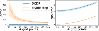
Figure 1: Average localization error and average run time versus the number of grid points $\mathcal{Q}$ over 100 trials. The shaded area indicates the upper and lower 0.1 quantiles of the corresponding quantities.

In the first set of experiments, we set $\Delta=5000,\delta=5$ and vary $\mathcal{Q}$ from $25$ to $200$, and summarize results in Figure 1. The left plot of the figure shows that while the localization errors of the divide step are sensitive to the choice of $\mathcal{Q}$, the additional conquer step (Algorithm 3) greatly improves the numerical accuracy of the final estimators of DCDP. The right plot of the figure demonstrates that the time complexity of DCDP is quadratic in $\mathcal{Q}$, which is in line with the complexity analysis presented in Section 2.

In the second set of experiments, we fix $\mathcal{Q}=100.\delta=5$ and let $\Delta$ range from 1000 to 6000. The results are summarized in Figure 2. The left plot of the figure shows that while the localization errors of the dive step change with $\Delta$, the accuracy of DCDP is consistently small for all the different values of $\Delta$. The right plot of the figure shows that the time complexity is linear in $n$, and this observation matches the findings presented in Section 2.

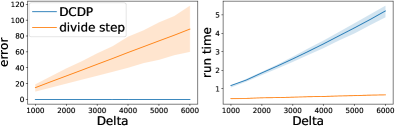
Figure 2: Average localization error and average run time v.s. $\Delta$ over 100 trials.

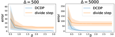
Figure 3: Localization error when varying $\delta$, the magnitude of nonzero signals.

Next, we fix $\mathcal{Q}=100$ and $\Delta\in\{500,5000\}$ and vary $\delta$, the strength of signals, to illustrate the performance of DCDP under different SNR levels. The results are summarized in Figure 3. More discussions on the accuracy under small $\delta$ are included in Section A.2.

4.2 Numerical performance of DCDP

Below we report the outcome of various simulation studies in which we compare the numerical performance of DCDP with that of several other state-of-the-art methods, for each of the three models presented in Section 3.

In the following experiments, for each specific $\Delta$ we set the total number of observations $n=(K+1)\Delta$ and the locations of true change points $\eta_{k}=k\Delta+\delta_{k}$, where $\delta_{k}$ is a random variable sampled from the uniform distribution ${\rm Unif}[-\frac{3}{10}\Delta,\frac{3}{10}\Delta]$. In each setting, we conduct 100 trials and report the average execution time, the average Hausdorff distance between true and estimated change points, and the frequency of cases in which $\widehat{K}=K$, for each method.

The mean model
We set $K=3$ and, for $k=0,\cdots,K$ and $\delta\in\{1,5\}$, we assume a population mean vector of the form

$${\bm{\mu}}^{*}_{\eta_{k}}=(\underbrace{0,\ldots,0}_{5k},\underbrace{\delta,\ldots,\delta}_{5},\underbrace{0,\ldots,0}_{p-5k-5})^{\top}\in\mathbb{R}^{p}.$$

We compare DCDP with Change-Forest (CF) (Londschien et al.,, 2022), Block-wise Fused Lasso (BFL) (Bai and Safikhani,, 2022), and Inspect (Wang and Samworth,, 2018). The results are summarized in Table 1. On average, DCDP outputs the most accurate change point estimators while remaining computationally efficient.

Method	$H(\hat{{\bm{\eta}}},{\bm{\eta}})$	Time	$\widehat{\mathbb{P}}[\widehat{K}=K]$
$n=200,p=100,K=3,\delta=5$
DCDP	0.00 (0.00)	0.6s (0.0)	1.00
Inspect	0.40 (3.50)	0.0s (0.0)	0.91
CF	1.84 (6.27)	0.8s (0.2)	0.90
BFL	47.84 (6.69)	1.4s (0.2)	0.00
$n=200,p=100,K=3,\delta=1$
DCDP	0.83 (0.87)	0.8s (0.2)	1.00
Inspect	2.65 (5.16)	0.0s (0.0)	0.86
CF	6.29 (9.57)	1.1s (0.3)	0.78
BFL	47.19 (6.48)	1.1s (0.2)	0.00

Table 1: Numerical comparison of different methods in the high-dimensional mean shift models. The numbers in the cells indicate the averages over 100 trials and the numbers in the brackets indicate the corresponding standard errors.

The linear regression model

We set $K=3$ and, for $k=0,\cdots,K$, assume population regression coefficients of the form

$${\bm{\beta}}^{*}_{\eta_{k}}=(\underbrace{0,\ldots,0}_{5k},\underbrace{\delta,\ldots,\delta}_{5},\underbrace{0,\ldots,0}_{p-5k-5})^{\top}\in\mathbb{R}^{p},$$

where $\delta\in\{1,5\}$.

We compare the numerical performance of DCDP with Variance-Projected Wild Binary Segmentation (VPBS) (Wang et al., 2021c, ) and vanilla Dynamic Programming (DP) (Rinaldo et al.,, 2021). The results are summarized in Table 2. On average, DCDP is the most efficient algorithm with compelling numerical accuracy.

Method	$H(\hat{{\bm{\eta}}},{\bm{\eta}})$	Time	$\widehat{\mathbb{P}}[\widehat{K}=K]$
$n=200,p=100,K=3,\delta=5$
DCDP	0.13 (0.39)	18.4s (1.1)	1.00
DP	0.01 (0.10)	220.3s (16.8)	0.98
VPWBS	15.44 (17.99)	120.1s (13.1)	0.70
$n=200,p=100,K=3,\delta=1$
DCDP	1.45 (8.59)	8.8s (0.7)	0.98
DP	0.22 (2.00)	84.4s (5.7)	0.99
VPWBS	11.54 (11.23)	120.4s (14.5)	0.65

Table 2: Numerical comparison of different methods in the high-dimensional regression coefficient shift models.

The Gaussian graphical model
We set $K=3$ and the population covariance matrix matrices as ${\bm{\Sigma}}^{*}_{\eta_{0}}={\bm{\Sigma}}^{*}_{\eta_{2}}={\bm{I}}_{p}$ and ${\bm{\Sigma}}^{*}_{\eta_{1}}={\bm{\Sigma}}^{*}_{\eta_{3}}$ where

$$({\bm{\Sigma}}^{*}_{\eta_{1}})_{ij}=({\bm{\Sigma}}^{*}_{\eta_{3}})_{ij}=\begin{cases}\delta_{1},&i=j;\\ \delta_{2},&|i-j|=1;\\ 0,&\text{otherwise},\end{cases}$$

with $\delta_{1}=5,\delta_{2}=0.3$.

We compare the numerical performance of DCDP with Change-Forest (CF) (Londschien et al.,, 2022) and Block-wise Fused Lasso (BFL) (Bai and Safikhani,, 2022). Note that the BFL algorithm produces empty set in all trials, so we only report DCDP and CF in Table 3. It can be seen that on average DCDP outputs the most accurate change point estimates and is highly computationally efficient.

Method	$H(\hat{{\bm{\eta}}},{\bm{\eta}})$	Time	$\widehat{\mathbb{P}}[\widehat{K}=K]$
$n=400,p=10,K=3,\delta_{1}=5,\delta_{2}=0.3$
DCDP	0.42 (0.64)	0.5s (0.0)	1.00
CF	5.54 (14.71)	0.6s (0.1)	0.88
$n=400,p=20,K=3,\delta_{1}=5,\delta_{2}=0.3$
DCDP	0.66 (4.37)	0.9s (0.3)	1.00
CF	7.37 (18.76)	1.0s (0.0)	0.85

Table 3: Numerical comparison of different methods in the precision matrix shift models.

4.3 Real data analysis

In this section, we apply DCDP to three popular real data examples and compare it with state-of-the-art methods.

Bladder tumor micro-array data. This dataset contains the micro-array records of 43 patients with bladder tumor, collected and studied by (Stransky et al.,, 2006). The result is visualized in Figure 4, where we only show the data of 10 patients for the ease of presentation and reading. While there is no accurate ground truth of locations of change points, the 37 change points spotted by DCDP align well with previous research (James and Matteson,, 2015; Wang and Samworth,, 2018). Figure 4 provides virtual support for the findings by DCDP.

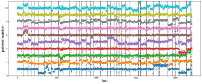
Figure 4: Estimated change points in the micro-array data. The result is based on the data of all 43 patients, while only the data of 10 patients is presented. The estimated change points are indicated by dashed vertical lines.

Dow Jones industrial average index. We apply DCDP to the weekly log return of the 29 companies composing the Dow Jones Industrial Average(DJIA) from April, 1990 to January, 2012, to detect changes in the covariance structure. We use the version of the data provided in (James and Matteson,, 2015). Two change points at September 22, 2008 and May 4, 2009 are detected, which correspond to the months during which the market was impacted by the financial crisis in 2008. The estimates by DCDP match well with previous research (James and Matteson,, 2015) on this data.

To give a virtual evaluation on estimated change points, in Figure 5 we show the estimated precision matrices on the three segments of the data split by the estimated change points.

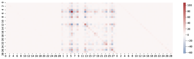
Figure 5: Estimated change points in the DJIA data.

FRED data. We also apply DCDP to Federal Reserve Economic Database (FRED) data. We use the subset of monthly data spanning from January 2000 to December 2019, which consists of $n=240$ samples. The original data has 128 features. We use the R package fbi(Yankang, Bennie) to transform the raw data to be stationary and remove outliers, as is suggested by the data collector (McCracken and Ng,, 2016). After preprocessing, there are 118 features, including the date.

We use logarithm of the monthly growth rate of the US industrial production index (named as INDPRO in the FRED data set) as the response variable, and other 116 macroeconomic variables as predictors. Previous research (Wang and Zhao,, 2022; Xu et al.,, 2022) suggests that there exist change points in the association between INDPRO and predictors.

DCDP spots a change point at January 2008, which is consistent with previous research on this data (Wang and Zhao,, 2022; Xu et al.,, 2022).

5 Discussion

In this paper, we propose a novel framework called DCDP for offline change point detection that can efficiently localize multiple change points for a broad range of high-dimensional models. DCDP improves the computational efficiency of vanilla dynamic programming while preserving the accuracy of change point estimation. DCDP serves as a unified methodology for a large family of change point models and theoretical guarantees for the localization errors of DCDP under three specific models are established. Extensive numerical experiments are conducted to compare the performance of DCDP with other popular methods to support our theoretical findings.

There are two main limitations in this paper. First, although the methodology itself is model-agnostic, we only consider linear-type models in the theoretical analysis. Thus, an important future direction is to generalize the theoretical analysis to other models like non-parametric families or artificial neural networks. Moreover, in our theoretical results, the sharpest localization error rates require stronger SNR conditions, as is discussed in Appendix F. Since there is no existing work in the literature achieving the same error rate with weaker assumptions, weakening the SNR conditions for the sharp error rate will be another important direction for future work.

Acknowledgments

We would like to thank the anonymous reviewers for their feedback which greatly helped improve our exposition. Wanshan Li and Alessandro Rinaldo acknowledge partial support from NSF grant DMS-EPSRC 2015489.

Appendix

The appendix contains seven parts. The first five parts present the proof of main results in Section 3 and the last two parts show some additional results of experiments on synthetic and real data. In detail,

1. Appendix A contains supplementary materials to numerical experiments in Section 4.

2. Appendix B contains key properties that make the proof of DCDP different from that of the vanilla DP. The computation complexity of the divide step is discussed in Lemma B.1.

3. Appendix C contains proof of Theorem 3.3 for the divide step under the mean model in Section 3.1.

4. Appendix D contains proof of Theorem 3.6 for the divide step under the linear model in Section 3.2.

5. Appendix E contains proof of Theorem 3.9 for the divide step under the Gaussian graphical model in Section 3.3.

6. Appendix F contains proof of Theorem 3.4, 3.7, 3.10 for the conquer step.

Appendix A Additional Experiments

This section serves as a supplement to Section 4. In Section A.1, we discuss the selection of $\gamma$. In Section A.3, we present full results of numerical experiments in Section 4.2.

A.1 Selection of $\gamma$

In the theory of DCDP, we need $\gamma=C_{\gamma}\mathcal{B}_{n}^{-1/2}\Delta_{\min}\kappa^{2}$, which involves unknown population parameter $\Delta_{\min}$ and $\kappa^{2}$. It is common in the change point literature and even broader literature that theoretically best tuning parameters involve unknown quantities, and a typical practical solution is to perform cross validation to select the best tuning parameter from a list of candidates.

Suppose we have data $\{\mathbf{Z}_{i}\}_{i\in[n]}$ with $\mathbf{Z}_{i}\sim\mathbb{P}_{{\bm{\theta}}_{i}}$. Without loss of generality, suppose $n=2m$ for some $m\in\mathbb{Z}^{+}$. We split the data by indices, such that data with odd indices $\{\mathbf{Z}_{2i-1}\}_{i\in[m]}$ is the training set and data with even indices $\{\mathbf{Z}_{2i}\}_{i\in[m]}$ is the test set. This is a common way to conduct cross validation in the change point literature. Given a set of candidate parameters $G=\{(\gamma_{i},\zeta_{i})\}_{i\in[l]}$, for each $i\in[l]$, the CV has three steps:

1. Run DCDP on $\{\mathbf{Z}_{2i-1}\}_{i\in\mathcal{I}_{k}}$ with $(\gamma_{i},\zeta_{i})$ to get a segmentation $\widetilde{P}=\{\mathcal{I}_{k}\}_{k\in[\widehat{K}+1]}$ of $[1,m]$ where $\mathcal{I}_{k}=[\widetilde{\eta}_{k-1},\widetilde{\eta}_{k})$.

2. Calculate $\{\widehat{{\bm{\theta}}}_{k}\}_{k\in[\widehat{K}+1]}$ from $\{\{\mathbf{Z}_{2i-1}\}_{i\in\mathcal{I}_{k}}\}_{k\in[\widehat{K}+1]}$ and

   $$R_{i}=\sum_{k\in[\widehat{K}+1]}\mathcal{F}(\widehat{{\bm{\theta}}}_{k},\mathcal{I}_{k})$$

   from $\{\{\mathbf{Z}_{2i}\}_{i\in\mathcal{I}_{k}}\}_{k\in[\widehat{K}+1]}$.

3. Select $(\gamma_{i_{cv}},\zeta_{i_{cv}})$ with the index $i_{cv}=\operatornamewithlimits{arg\,min}_{i\in[l]}R_{i}$.

A.2 Impact of SNR

In Section 4.1, we illustrate the performance of DCDP with varying SNR levels. As is shown in Figure 3, the localization error gets larger when $\delta$, the signal strength, becomes smaller. In this section, we show that the localization errors of DCDP for small $\delta$ are in fact reasonably good. The data generating mechanism is the same as in Section 4.1.

We set $\Delta=500$. In the left panel of Figure 6, we set $n=2\Delta$ and allow the estimator to know that there is a single change point, which is the simplest setting of change point detection. In this setting, the optimal estimator is to simply pick the extreme point of the CUSUM statistic. It can be seen that with similar SNR, the localization error of DCDP under the (much more difficult) multiple change point setting is only twice of the error of the most powerful method in the simplest case. This demonstrate that DCDP performs well in low SNR scenarios.

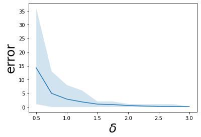
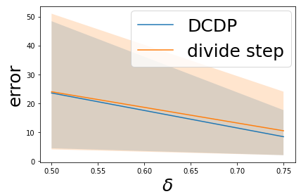
Figure 6: Left: localization error of the extreme point of the CUSUM statistic when $n=2\Delta$ and it is known that there is only one change point; right: localization error of DCDP when $\mathcal{Q}=n$ under $n=4\Delta$ and $\delta\in\{0.50,0.75\}$.

In the right panel of Figure 6, we set $n=4\Delta$ (i.e., there are 3 change points) and let $\mathcal{Q}=n$, $\delta\in\{0.50,0.75\}$. In this setting, the "divide step" corresponds to the vanilla DP and "DCDP" corresponds to vanilla DP + local refinement. Theoretically, this would lead to more accurate estimates, but with a much higher computational price. However, comparing the resulted errors with those in Figure 3, it can be seen that the improvement on the localization error against that of $\mathcal{Q}=100$ is fairly small, while the actual run time is more than 200 times longer. This demonstrates that DCDP is efficient and accurate, even when the SNR is low.

A.3 More results on comparisons

In this section we present full results of comparisons between DCDP and other methods in Table 4, Table 5, and Table 6, as a supplement to Section 4.2. Among all involved methods, DCDP is implemented in Python, ChangeForest is implemented in Rust and provides Python API, Inspect, Variance-Projected WBS, vanilla DP, and Block-Fused-Lasso are implemented in R based on Rcpp. For fair comparison, we first generate data in Python and then load the data in R for R-based methods. All experiments for DCDP and ChangeForest are run on a virtual machine of Google Colab with Intel(R) Xeon(R) CPU of 2 cores 2.30 GHz and 12GB RAM (one setting at a time). All other experiments are run on a personal computer with Intel Core i7 8850H CPU of 6 cores 2.60GHz and 64GB RAM (one setting at a time). Notice that programs implemented by Rcpp is usually faster than Python, and the machine to run Rcpp-based methods has better parameters than the virtual machine to run DCDP and ChangeForest, the comparison of execution time would not be unfair against Rcpp-based methods.

Table 4 shows full results of the comparison under the mean shift model.

Setting	Method	$H(\hat{\eta},\eta)$	Time	$\hat{K}<K$	$\hat{K}=K$	$\hat{K}>K$
$n=200,p=20,K=3,\delta=5$	DCDP	0.00 (0.00)	0.7s (0.2)	0	100	0
	Inspect	0.54 (4.46)	0.0s (0.0)	0	96	4
	CF	3.59 (10.10)	0.3s (0.0)	0	84	16
	BFL	42.56 (6.95)	3.5s (0.6)	100	0	0
$n=200,p=20,K=3,\delta=1$	DCDP	0.51 (0.77)	0.7s (0.2)	0	100	0
	Inspect	3.13 (5.50)	0.0s (0.0)	0	67	33
	CF	4.38 (10.13)	0.4s (0.1)	0	81	19
	BFL	43.30 (8.25)	2.9s (0.6)	100	0	0
$n=200,p=20,K=3,\delta=0.5$	DCDP	8.30 (12.90)	0.4s (0.0)	8	90	2
	Inspect	6.85 (7.53)	0.0s (0.0)	0	78	22
	CF	7.15 (9.57)	0.4s (0.1)	1	78	21
	BFL	54.48 (20.98)	2.8s (1.1)	100	0	0
$n=200,p=100,K=3,\delta=5$	DCDP	0.0 (0.0)	0.6s (0.0)	0	100	0
	Inspect	0.40 (3.50)	0.0s (0.0)	0	91	9
	CF	2.85 (7.50)	0.8s (0.2)	0	85	15
	BFL	47.80 (6.66)	1.5s (0.3)	100	0	0
$n=200,p=100,K=3,\delta=1$	DCDP	0.83 (0.87)	0.8s (0.2)	0	100	0
	Inspect	2.65 (5.16)	0.0s (0.0)	0	86	14
	CF	3.28 (7.01)	1.3s (0.1)	0	85	15
	BFL	47.59 (6.08)	1.1s (0.2)	100	0	0
$n=800,p=100,K=3,\delta=0.5$	DCDP	9.36 (29.96)	2.1s (0.3)	3	97	0
	Inspect	12.55 (22.14)	0.1s (0.0)	0	77	23
	CF	14.73 (30.50)	5.5s (0.3)	0	82	18
	BFL	80.10 (137.33)	15.7s (3.8)	28	71	1

Table 4: Comparison of DCDP and other methods under the mean model with different simulation settings. 100 trials are conducted in each setting. For the localization error and running time (in seconds), the average over 100 trials is shown with standard error in the bracket. The three columns on the right record the number of trials in which $\hat{K}<K$, $\hat{K}=K$, and $\hat{K}>K$ respectively.

Table 5 shows full results of the comparison under the linear regression coefficient shift model.

Setting	Method	$H(\hat{\eta},\eta)$	Time	$\hat{K}<K$	$\hat{K}=K$	$\hat{K}>K$
$n=200,p=20,K=3,\delta=5$	DCDP	0.03 (0.17)	5.1s (0.3)	0	100	0
	DP	0.04 (0.20)	17.0s (0.5)	0	100	0
	VPWBS	7.69 (15.53)	28.4s (3.5)	1	71	28
	BFL	84.45 (15.33)	4.2s (0.7)	100	0	0
$n=200,p=20,K=3,\delta=1$	DCDP	0.94 (5.17)	2.3s (0.2)	2	98	0
	DP	0.05 (0.22)	12.8s (0.5)	0	100	0
	VPWBS	11.71 (19.82)	30.4s (2.2)	21	73	6
	BFL	43.31 (8.82)	3.1s (0.8)	100	0	0
$n=200,p=100,K=3,\delta=5$	DCDP	0.13 (0.39)	18.4s (1.1)	0	100	0
	DP	0.01 (0.10)	220.3s (16.8)	0	98	2
	VPWBS	15.44 (17.99)	120.1s (13.1)	18	70	12
	BFL	47.84 (6.69)	1.4s (0.2)	100	0	0
$n=200,p=100,K=3,\delta=1$	DCDP	1.45 (8.59)	8.8s (0.7)	2	98	0
	DP	0.22 (2.00)	84.4s (5.7)	0	99	1
	VPWBS	11.54 (11.23)	120.4s (14.5)	3	65	32
	BFL	47.19 (6.48)	1.1s (0.2)	100	0	0

Table 5: Comparison of DCDP and other methods under the linear model with different simulation settings. 100 trials are conducted in each setting. For the localization error and running time (in seconds), the average over 100 trials is shown with standard error in the bracket. The three columns on the right record the number of trials in which $\hat{K}<K$, $\hat{K}=K$, and $\hat{K}>K$ respectively.

Table 6 shows full results of the comparison under the precision shift model. In Table 6, we didn’t present the results of BFL because it produces empty set in all trials, for some unknown reason. We tried to fine tune the parameters in BFL, but didn’t manage to produce nonempty sets, probably because the precision matrices under our setting are not sparse enough for BFL to perform well.

Setting	Method	$H(\hat{\eta},\eta)$	Time	$\hat{K}<K$	$\hat{K}=K$	$\hat{K}>K$
$n=2000,p=5,K=3,\delta_{1}=2,\delta_{2}=0.3$	DCDP	5.16 (6.52)	0.7s (0.3)	0	100	0
	CF	58.25 (151.74)	1.8s (0.3)	2	69	29
$n=2000,p=10,K=3,\delta_{1}=5,\delta_{2}=0.3$	DCDP	0.27 (0.49)	0.7s (0.1)	0	100	0
	CF	42.5 (137.92)	2.9s (0.2)	0	84	16
$n=2000,p=20,K=3,\delta_{1}=5,\delta_{2}=0.3$	DCDP	0.03 (0.17)	1.2s (0.2)	0	100	0
	CF	27.68 (97.20)	4.8s (0.4)	0	86	14
$n=400,p=10,K=3,\delta_{1}=5,\delta_{2}=0.3$	DCDP	0.42 (0.64)	0.5s (0.0)	0	100	0
	CF	5.54 (14.71)	0.6s (0.1)	0	88	12
$n=400,p=20,K=3,\delta_{1}=5,\delta_{2}=0.3$	DCDP	0.66 (4.37)	0.9s (0.3)	0	100	0
	CF	7.37 (18.76)	1.0s (0.0)	0	85	15

Table 6: Comparison of DCDP and other methods under the covariance model with different simulation settings. 100 trials are conducted in each setting. For the localization error and running time (in seconds), the average over 100 trials is shown with standard error in the bracket. The three columns on the right record the number of trials in which $\hat{K}<K$, $\hat{K}=K$, and $\hat{K}>K$ respectively.

Appendix B Fundamental lemma

In the proof of localization error of the vanilla dynamic programming, we frequently compare the goodness-of-fit function $\mathcal{F}(\widehat{\theta}_{\mathcal{I}},\mathcal{I})$ over an interval $\mathcal{I}=(s,e]$ with

$$\mathcal{F}(\widehat{\theta}_{(s,\eta_{i+1}]},(s,\eta_{i+1}])+\cdots+\mathcal{F}(\widehat{\theta}_{(\eta_{i+m},e]},(\eta_{i+m},e])+m\gamma$$ (B.1)

where $\{\eta_{i+j}\}_{j\in[m]}=\{\eta_{\ell}\}_{\ell\in[K]}\cap\mathcal{I}$ is the collection of true change points within interval $\mathcal{I}$ and $\gamma$ is the penalty tuning parameter of the DP.

However, for DCDP, we only search over the rough grid $\{s_{i}=\lfloor\frac{i\cdot n}{\mathcal{Q}+1}\rfloor\}_{i\in[\mathcal{Q}]}$ that may or may not contain any true change points. Therefore, we need to a) guarantee the existence of some reference points (contained in $\{s_{i}\}_{i\in[\mathcal{Q}]}$) that are close enough to true change points, and b) quantify the deviation of the goodness-of-fit function evaluated at the reference points compared to that evaluated at the true change points.

Reference points.

The grid is given by points $s_{q}=\lfloor\frac{q\cdot n}{\mathcal{Q}+1}\rfloor$ for $q\in[{\mathcal{Q}}]$. Let $\{\eta_{k}\}_{k\in[K]}$ be the collection of change points and denote

$$\mathcal{L}_{k}(\delta):=\bigg{\{}\{s_{q}\}_{q\in[{\mathcal{Q}}]}\bigcap[\eta_{k}-\delta,\eta_{k}]\not=\emptyset\bigg{\}},\quad\text{and}\quad\mathcal{R}_{k}(\delta):=\bigg{\{}\{s_{q}\}_{q\in[{\mathcal{Q}}]}\bigcap[\eta_{k},\eta_{k}+\delta]\not=\emptyset\bigg{\}}.$$

Intuitively, if $s_{q}\in[\eta_{k}-\delta,\eta_{k}]$ and $s_{q^{\prime}}\in[\eta_{k},\eta_{k}+\delta]$ , then $s_{q},s_{q^{\prime}}$ can serve as reference points of the true change point $\eta_{k}$. Denote

$$\mathcal{L}(\delta):=\bigcap_{k=1}^{K}\mathcal{L}_{k}\big{(}\delta\big{)}\quad\text{and}\quad\mathcal{R}(\delta):=\bigcap_{k=1}^{K}\mathcal{R}_{k}\big{(}\delta\big{)}.$$ (B.2)

Then it is straightforward to see that both events $\mathcal{L}(\delta)$ and $\mathcal{R}(\delta)$ will hold as long as $\min_{q\in[\mathcal{Q}+1]}|s_{q}-s_{q-1}|<\frac{\delta}{2}$, which is guaranteed if $\mathcal{Q}>3\frac{n}{\delta}$. For the proofs in Appendix C, Appendix D, and Appendix E, we require that $\mathcal{L}(\mathcal{B}_{n}^{-1}\Delta_{\min})$ and $\mathcal{R}(\mathcal{B}_{n}^{-1}\Delta_{\min})$ hold. Therefore, for the theoretical results in Section 3 to hold, $\mathcal{Q}$ should satisfy that

$$\mathcal{Q}>\frac{3n}{\Delta_{\min}}\mathcal{B}_{n}.$$

Since in our paper, $\{\mathcal{B}_{n}\}_{n\in\mathcal{Z}^{+}}$ is a slowly diverging sequence, we can take it as $\mathcal{B}_{n}=\log(n)$ and then it suffices to take $\mathcal{Q}=\frac{4n}{\Delta_{\min}}\log^{2}(n)$.

Under the fixed-$K$ setting of paper and when $\{\Delta_{k}\}_{k\in[K]}$ are of the same order, the existence of reference points will be guaranteed as long as $\mathcal{Q}>4\log^{2}(n)$.

Goodness-of-fit.

The deviation of goodness-of-fit functions at reference points are different from the one that occurs in the proof of the vanilla DP, because the fitted parameters would have some bias since reference points may not locate at true change points. For different models, the deviation of the goodness-of-fit has different orders. We need to analyze each model separately. The deviations are described in Lemma C.4, Lemma D.4, and Lemma E.4.

Complexity analysis.

In Lemma B.1 we analyze the complexity of the divide step.

Lemma B.1 (Complexity of the divide step).

Under all three models in Section 3, with a memorization technique, the computation complexity of Algorithm 2 would be $O(n\mathcal{Q}\cdot\mathcal{C}_{2}(p))$.

Proof.

For generality, suppose $\{s_{i}\}_{i\in[\mathcal{Q}]}$ is an arbitrary grid of integers over $(0,n)$, i.e., $0<s_{1}<s_{2}<\cdots<s_{\mathcal{Q}}<n$, and denote $s_{0}=0$, $s_{\mathcal{Q}+1}=n$, $\delta_{i}=s_{i}-s_{i-1}$ for $i\in[\mathcal{Q}+1]$.

Under the three models in Section 3, calculating $\widehat{\theta}_{\mathcal{I}}$ only involves summations like $\sum_{i\in\mathcal{I}}X_{i}$, $\sum_{i\in\mathcal{I}}X_{i}X_{i}^{\top}$, $\sum_{i\in\mathcal{I}}X_{i}y_{i}$. In $l$-th step ($l\geq 1$) of the inner loop of Algorithm 2 at the right end point $s_{r}$, it suffices to remove $\delta_{l}$ terms from the summation. Thus, the complexity for the inner loop at $s_{r}$ would be $O(s_{r}\cdot\mathcal{C}_{2}(p))$, and the total complexity would be

$$\sum_{r\in[\mathcal{Q}]}O(s_{r}\cdot\mathcal{C}_{2}(p))=O(n\mathcal{Q}\cdot\mathcal{C}_{2}(p)).$$

∎

Appendix C Mean model

In this section we show the proof of Theorem 3.3. Throughout this section, for any generic interval ${\mathcal{I}}\subset[1,n]$, denote $\mu^{*}_{{\mathcal{I}}}=\frac{1}{|{\mathcal{I}}|}\sum_{i\in{\mathcal{I}}}\mu^{*}_{i}$ and

$$\widehat{\mu}_{\mathcal{I}}=\operatornamewithlimits{arg\,min}_{\mu\in\mathbb{R}^{p}}\frac{1}{|\mathcal{I}|}\sum_{i\in\mathcal{I}}\|X_{i}-\mu\|_{2}^{2}+\frac{\lambda}{\mathchoice{{\hbox{$\displaystyle\sqrt{|\mathcal{I}|\,}$}\lower 0.4pt\hbox{\vrule height=7.5pt,depth=-6.00003pt}}}{{\hbox{$\textstyle\sqrt{|\mathcal{I}|\,}$}\lower 0.4pt\hbox{\vrule height=7.5pt,depth=-6.00003pt}}}{{\hbox{$\scriptstyle\sqrt{|\mathcal{I}|\,}$}\lower 0.4pt\hbox{\vrule height=5.25pt,depth=-4.20003pt}}}{{\hbox{$\scriptscriptstyle\sqrt{|\mathcal{I}|\,}$}\lower 0.4pt\hbox{\vrule height=3.75pt,depth=-3.00002pt}}}}\|\mu\|_{1}.$$

Also, unless specially mentioned, in this section, we set the goodness-of-fit function $\mathcal{F}({\mathcal{I}})$ in Algorithm 1 to be

$$\mathcal{F}({\mathcal{I}}):=\begin{cases}\sum_{i\in{\mathcal{I}}}\|X_{i}-\widehat{\mu}_{\mathcal{I}}\|_{2}^{2},&\text{ when }|{\mathcal{I}}|\geq C_{\mathcal{F}}\sigma_{\epsilon}^{2}{\mathfrak{s}}\log(n\vee p),\\ 0,&\text{otherwise},\end{cases}.$$ (C.1)

where $C_{\mathcal{F}}$ is a universal constant.

Assumptions.

For the ease of presentation, we combine the SNR condition we will use throughout this section and Assumption 3.2 into a single assumption.

Assumption C.1 (Mean model).

Suppose that Assumption 3.2 holds. In addition, suppose that $\Delta_{\min}\kappa^{2}\geq\mathcal{B}_{n}\mathfrak{s}\log(n\vee p)$ as is assumed in Theorem 3.3.

Proof of Theorem 3.3.

By Proposition C.2, $K\leq|\widehat{\mathcal{P}}|\leq 3K$. This combined with Proposition C.3 completes the proof. ∎

Proposition C.2.

Suppose Assumption C.1 holds. Let $\widehat{\mathcal{P}}$ denote the output of Algorithm 1. Then with probability at least $1-Cn^{-3}$, the following conditions hold.

• For each interval ${\mathcal{I}}=(s,e]\in\widehat{\mathcal{P}}$ containing one and only one true change point $\eta_{k}$, it must be the case that

  $$\min\{\eta_{k}-s,e-\eta_{k}\}\lesssim\sigma_{\epsilon}^{2}\bigg{(}\frac{{\mathfrak{s}}\log(n\vee p)+\gamma}{\kappa_{k}^{2}}\bigg{)}+{\mathcal{B}_{n}^{-1}\Delta_{\min}}.$$

• For each interval ${\mathcal{I}}=(s,e]\in\widehat{\mathcal{P}}$ containing exactly two true change points, say $\eta_{k}<\eta_{k+1}$, it must be the case that

  $$\eta_{k}-s\lesssim{\mathcal{B}_{n}^{-1/2}\Delta_{\min}}\quad\text{and}\quad e-\eta_{k+1}\lesssim{\mathcal{B}_{n}^{-1/2}\Delta_{\min}}.$$

• No interval ${\mathcal{I}}\in\widehat{\mathcal{P}}$ contains strictly more than two true change points.

• For all consecutive intervals ${\mathcal{I}}_{1}$ and ${\mathcal{I}}_{2}$ in $\widehat{\mathcal{P}}$, the interval ${\mathcal{I}}_{1}\cup{\mathcal{I}}_{2}$ contains at least one true change point.

Proof.

The four cases are proved in Lemma C.7, Lemma C.8, Lemma C.9, and Lemma C.10, respectively. ∎

Proposition C.3.

Suppose Assumption C.1 holds. Let $\widehat{\mathcal{P}}$ be the output of Algorithm 1. Suppose $\gamma\geq C_{\gamma}K{\mathcal{B}_{n}^{-1}\Delta_{\min}}\kappa^{2}$ for sufficiently large constant $C_{\gamma}$. Then with probability at least $1-Cn^{-3}$, $|\widehat{\mathcal{P}}|=K$.

Proof of Proposition C.3.

Denote $\mathfrak{G}^{*}_{n}=\sum_{i=1}^{n}\|X_{i}-\mu^{*}_{i}\|_{2}^{2}$. Given any collection $\{t_{1},\ldots,t_{m}\}$, where $t_{1}<\cdots<t_{m}$, and $t_{0}=0$, $t_{m+1}=n$, let

$${\mathfrak{G}}_{n}(t_{1},\ldots,t_{m})=\sum_{k=1}^{m}\mathcal{F}(\widehat{\mu}_{(t_{k},t_{k+1}]},(t_{k},t_{k+1}]).$$ (C.2)

For any collection of time points, when defining (C.2), the time points are sorted in an increasing order.

Let $\{\widehat{\eta}_{k}\}_{k=1}^{\widehat{K}}$ denote the change points induced by $\widehat{\mathcal{P}}$. Suppose we can justify that

$${\mathfrak{G}}^{*}_{n}+K\gamma\geq {\mathfrak{G}}_{n}(s_{1},\ldots,s_{K})+K\gamma-C_{1}(K+1)\sigma_{\epsilon}^{2}{\mathfrak{s}}\log(n\vee p)-C_{1}\sum_{k\in[K]}\kappa_{k}^{2}{\mathcal{B}_{n}^{-1}\Delta_{\min}}$$ (C.3)

$$\geq {\mathfrak{G}}_{n}(\widehat{\eta}_{1},\ldots,\widehat{\eta}_{\widehat{K}})+\widehat{K}\gamma-C_{1}(K+1)\sigma_{\epsilon}^{2}{\mathfrak{s}}\log(n\vee p)-C_{1}\sum_{k\in[K]}\kappa_{k}^{2}{\mathcal{B}_{n}^{-1}\Delta_{\min}}$$ (C.4)

$$\geq {\mathfrak{G}}_{n}(\widehat{\eta}_{1},\ldots,\widehat{\eta}_{\widehat{K}},\eta_{1},\ldots,\eta_{K})+\widehat{K}\gamma-2C_{1}(K+1)\sigma_{\epsilon}^{2}{\mathfrak{s}}\log(n\vee p)-C_{1}\sum_{k\in[K]}\kappa_{k}^{2}{\mathcal{B}_{n}^{-1}\Delta_{\min}}$$ (C.5)

and that

$${\mathfrak{G}}^{*}_{n}-{\mathfrak{G}}_{n}(\widehat{\eta}_{1},\ldots,\widehat{\eta}_{\widehat{K}},\eta_{1},\ldots,\eta_{K})\leq C_{2}(K+\widehat{K}+2)\sigma_{\epsilon}^{2}{\mathfrak{s}}\log(n\vee p).$$ (C.6)

Then it must hold that $|\mathcal{P}|=K$, as otherwise if $\widehat{K}\geq K+1$, then

$$C_{2}(K+\widehat{K}+2)\sigma_{\epsilon}^{2}{\mathfrak{s}}\log(n\vee p) \geq{\mathfrak{G}}^{*}_{n}-{\mathfrak{G}}_{n}(\widehat{\eta}_{1},\ldots,\widehat{\eta}_{\widehat{K}},\eta_{1},\ldots,\eta_{K})$$

$$\geq(\widehat{K}-K)\gamma-2C_{1}(K+1)\sigma_{\epsilon}^{2}{\mathfrak{s}}\log(n\vee p)-2C_{1}\sum_{k\in[K]}\kappa_{k}^{2}{\mathcal{B}_{n}^{-1}\Delta_{\min}}.$$

Therefore due to the assumption that $|\widehat{p}|=\widehat{K}\leq 3K$, it holds that

$$[C_{2}(4K+2)+2C_{1}(K+1)]\sigma_{\epsilon}^{2}{\mathfrak{s}}\log(n\vee p)+2C_{1}\sum_{k\in[K]}\kappa_{k}^{2}{\mathcal{B}_{n}^{-1}\Delta_{\min}}\geq(\widehat{K}-K)\gamma\geq\gamma,$$ (C.7)

Note that (C.7) contradicts the choice of $\gamma$.

Step 1. Note that (C.3) is implied by

$$\left|{\mathfrak{G}}^{*}_{n}-{\mathfrak{G}}_{n}(s_{1},\ldots,s_{K})\right|\leq C_{3}(K+1)\sigma_{\epsilon}^{2}{\mathfrak{s}}\log(n\vee p)+C_{3}\sum_{k\in[K]}\kappa_{k}^{2}{\mathcal{B}_{n}^{-1}\Delta_{\min}},$$ (C.8)

which is an immediate consequence of Lemma C.4.  

Step 2. Since $\{\widehat{\eta}_{k}\}_{k=1}^{\widehat{K}}$ are the change points induced by $\widehat{\mathcal{P}}$, (C.4) holds because $\widehat{\mathcal{P}}$ is a minimizer.
Step 3. For every ${\mathcal{I}}=(s,e]\in\widehat{p}$, by Proposition C.2, we know that ${\mathcal{I}}$ contains at most two change points. We only show the proof for the two-change-points case as the other case is easier. Denote

$${\mathcal{I}}=(s,\eta_{q}]\cup(\eta_{q},\eta_{q+1}]\cup(\eta_{q+1},e]={\mathcal{J}}_{1}\cup{\mathcal{J}}_{2}\cup{\mathcal{J}}_{3},$$ (C.9)

where $\{\eta_{q},\eta_{q+1}\}={\mathcal{I}}\,\cap\,\{\eta_{k}\}_{k=1}^{K}$.

For each $m=1,2,3$, if $|{\mathcal{J}}_{m}|\geq C_{\mathcal{F}}\sigma_{\epsilon}^{2}{\mathfrak{s}}\log(n\vee p)$, then by Lemma C.4, it holds that

$$\sum_{i\in{\mathcal{J}}_{m}}\|y_{i}-\widehat{\mu}_{{\mathcal{J}}_{m}}\|_{2}^{2}\leq\sum_{i\in{\mathcal{J}}_{m}}\|y_{i}-\mu^{*}_{i}\|_{2}^{2}+C\sigma_{\epsilon}^{2}{\mathfrak{s}}\log(n\vee p).$$

Thus, we have

$$\mathcal{F}(\widehat{\mu}_{{\mathcal{J}}_{m}},{\mathcal{J}}_{m})\leq\mathcal{F}(\mu^{*}_{{\mathcal{J}}_{m}},{\mathcal{J}}_{m})+C\sigma_{\epsilon}^{2}{\mathfrak{s}}\log(n\vee p).$$ (C.10)

On the other hand, by Lemma C.6, we have

$$\mathcal{F}(\widehat{\mu}_{{\mathcal{I}}},{\mathcal{J}}_{m})\geq\mathcal{F}(\mu^{*}_{{\mathcal{J}}_{m}},{\mathcal{J}}_{m})-C\sigma_{\epsilon}^{2}{\mathfrak{s}}\log(n\vee p).$$

Therefore the last two inequalities above imply that

$$\mathcal{F}(\widehat{\mu}_{\mathcal{I}},{\mathcal{I}})\geq \sum_{m=1}^{3}\mathcal{F}(\widehat{\mu}_{\mathcal{I}},{\mathcal{J}}_{m})$$

$$\geq \sum_{m=1}^{3}\mathcal{F}(\widehat{\mu}_{{\mathcal{J}}_{m}},{\mathcal{J}}_{m})-6C\sigma_{\epsilon}^{2}{\mathfrak{s}}\log(n\vee p).$$ (C.11)

Note that (C.5) is an immediate consequence of (C.11).

Step 4. Finally, to show (C.6), let $\widetilde{\mathcal{P}}$ denote the partition induced by $\{\widehat{\eta}_{1},\ldots,\widehat{\eta}_{\widehat{K}},\eta_{1},\ldots,\eta_{K}\}$. Then $|\widetilde{\mathcal{P}}|\leq K+\widehat{K}+2$ and that $\mu^{*}_{i}$ is unchanged in every interval ${\mathcal{I}}\in\widetilde{\mathcal{P}}$. So Equation C.6 is an immediate consequence of Lemma C.4. ∎

C.1 Fundamental lemmas

Lemma C.4 (Deviation, mean model).

Let $\mathcal{I}=(s,e]\subset(0,n]$ be any generic interval and

$$\widehat{\mu}_{\mathcal{I}}=\operatornamewithlimits{arg\,min}_{\mu}\frac{1}{|\mathcal{I}|}\sum_{i\in\mathcal{I}}\|X_{i}-\mu\|_{2}^{2}+\frac{\lambda}{\mathchoice{{\hbox{$\displaystyle\sqrt{|\mathcal{I}|\,}$}\lower 0.4pt\hbox{\vrule height=7.5pt,depth=-6.00003pt}}}{{\hbox{$\textstyle\sqrt{|\mathcal{I}|\,}$}\lower 0.4pt\hbox{\vrule height=7.5pt,depth=-6.00003pt}}}{{\hbox{$\scriptstyle\sqrt{|\mathcal{I}|\,}$}\lower 0.4pt\hbox{\vrule height=5.25pt,depth=-4.20003pt}}}{{\hbox{$\scriptscriptstyle\sqrt{|\mathcal{I}|\,}$}\lower 0.4pt\hbox{\vrule height=3.75pt,depth=-3.00002pt}}}}\|\mu\|_{1}.$$

a. If ${\mathcal{I}}$ contains no change points, then it holds that

$$\mathbb{P}\bigg{(}\bigg{|}\sum_{i\in{\mathcal{I}}}\|X_{i}-\widehat{\mu}_{\mathcal{I}}\|_{2}^{2}-\sum_{i\in{\mathcal{I}}}\|X_{i}-\mu^{*}_{i}\|_{2}^{2}\bigg{|}\geq C\sigma_{\epsilon}^{2}\mathfrak{s}\log(n\vee p)\bigg{)}\leq(n\vee p)^{-3}.$$

b. Suppose that the interval ${\mathcal{I}}$ contains one and only one change point $\eta_{k}$. Denote

$$\mathcal{J}=(s,\eta_{k}]\quad\text{and}\quad\mathcal{J}^{\prime}=(\eta_{k},e].$$

Then it holds that

$$\mathbb{P}\bigg{(}\bigg{|}\sum_{i\in{\mathcal{I}}}\|X_{i}-\widehat{\mu}_{\mathcal{I}}\|^{2}-\sum_{i\in{\mathcal{I}}}\|X_{i}-\mu^{*}_{i}\|^{2}\bigg{|}\geq 2\frac{|{\mathcal{J}}||{\mathcal{J}}^{\prime}|}{|{\mathcal{I}}|}\kappa_{k}^{2}+C\sigma_{\epsilon}^{2}\mathfrak{s}\log(n\vee p)\bigg{)}\leq(n\vee p)^{-3}.$$

Proof.

We show b as a immediately follows from b with $|{\mathcal{J}}^{\prime}|=0$. Denote

$$\mathcal{J}=(s,\eta_{k}]\quad\text{and}\quad\mathcal{J}^{\prime}=(\eta_{k},e].$$

Denote $\mu_{\mathcal{I}}=\frac{1}{|{\mathcal{I}}|}\sum_{i\in{\mathcal{I}}}\mu^{*}_{i}$. The it holds that

$$\begin{split}&\sum_{i\in{\mathcal{I}}}\|X_{i}-\widehat{\mu}_{\mathcal{I}}\|_{2}^{2}-\sum_{i\in{\mathcal{I}}}\|X_{i}-\mu^{*}_{i}\|_{2}^{2}\\ =&\sum_{i\in{\mathcal{I}}}\|\widehat{\mu}_{\mathcal{I}}-\mu^{*}_{i}\|_{2}^{2}-2\sum_{i\in{\mathcal{I}}}\epsilon_{i}^{\top}(\widehat{\mu}_{\mathcal{I}}-\mu^{*}_{i})\\ \leq&2\sum_{i\in{\mathcal{I}}}\|\widehat{\mu}_{\mathcal{I}}-\mu^{*}_{\mathcal{I}}\|_{2}^{2}+2\sum_{i\in{\mathcal{I}}}\|\mu^{*}_{\mathcal{I}}-\mu^{*}_{i}\|_{2}^{2}-2\sum_{i\in{\mathcal{I}}}\epsilon_{i}^{\top}(\widehat{\mu}_{\mathcal{I}}-\mu^{*}_{\mathcal{I}})-2\sum_{i\in{\mathcal{I}}}\epsilon_{i}^{\top}(\mu^{*}_{\mathcal{I}}-\mu^{*}_{i}).\end{split}$$

Observe that

$$\mathbb{P}\bigg{(}\|\sum_{i\in{\mathcal{I}}}\epsilon_{i}\|_{\infty}\geq C\sigma_{\epsilon}\mathchoice{{\hbox{$\displaystyle\sqrt{\log(n\vee p)|{\mathcal{I}}|\,}$}\lower 0.4pt\hbox{\vrule height=7.5pt,depth=-6.00003pt}}}{{\hbox{$\textstyle\sqrt{\log(n\vee p)|{\mathcal{I}}|\,}$}\lower 0.4pt\hbox{\vrule height=7.5pt,depth=-6.00003pt}}}{{\hbox{$\scriptstyle\sqrt{\log(n\vee p)|{\mathcal{I}}|\,}$}\lower 0.4pt\hbox{\vrule height=5.25pt,depth=-4.20003pt}}}{{\hbox{$\scriptscriptstyle\sqrt{\log(n\vee p)|{\mathcal{I}}|\,}$}\lower 0.4pt\hbox{\vrule height=3.75pt,depth=-3.00002pt}}}\bigg{)}\leq(n\vee p)^{-5}$$

Suppose this good event holds.

Step 1. By the event and Lemma C.5, we have

$$\begin{split}\sum_{i\in{\mathcal{I}}}\|\widehat{\mu}_{\mathcal{I}}-\mu^{*}_{\mathcal{I}}\|_{2}^{2}&\leq C\sigma_{\epsilon}^{2}{\mathfrak{s}}\log(n\vee p),\\ |2\sum_{i\in{\mathcal{I}}}\epsilon_{i}^{\top}(\widehat{\mu}_{\mathcal{I}}-\mu^{*}_{\mathcal{I}})|&\leq|{\mathcal{I}}|\|\sum_{i\in{\mathcal{I}}}\epsilon_{i}\|_{\infty}\|\widehat{\mu}_{\mathcal{I}}-\mu^{*}_{\mathcal{I}}\|_{1}\leq C\sigma_{\epsilon}^{2}{\mathfrak{s}}\log(n\vee p).\end{split}$$

Step 2. Notice that

$$\sum_{i\in{\mathcal{I}}}\|\mu^{*}_{\mathcal{I}}-\mu^{*}_{i}\|^{2}= \sum_{i\in{\mathcal{I}}}\|\frac{|{\mathcal{J}}|\mu^{*}_{\mathcal{J}}+|{\mathcal{J}}^{\prime}|\mu^{*}_{{\mathcal{J}}^{\prime}}}{|{\mathcal{I}}|}-\mu^{*}_{i}\|_{2}^{2}$$

$$= \sum_{i\in{\mathcal{J}}}\|\frac{|{\mathcal{J}}^{\prime}|(\mu^{*}_{\mathcal{J}}-\mu^{*}_{{\mathcal{J}}^{\prime}})}{|{\mathcal{I}}|}\|_{2}^{2}+\sum_{i\in{\mathcal{J}}^{\prime}}\|\frac{|{\mathcal{J}}|(\mu^{*}_{\mathcal{J}}-\mu^{*}_{{\mathcal{J}}^{\prime}})}{|{\mathcal{I}}|}\|_{2}^{2}$$

$$= \frac{|{\mathcal{J}}||{\mathcal{J}}^{\prime}|}{|{\mathcal{I}}|}\|\mu^{*}_{\mathcal{J}}-\mu^{*}_{{\mathcal{J}}^{\prime}}\|_{2}^{2}=\frac{|{\mathcal{J}}||{\mathcal{J}}^{\prime}|}{|{\mathcal{I}}|}\kappa_{k}^{2}.$$

Meanwhile, it holds that

$$\sum_{i\in{\mathcal{I}}}\epsilon_{i}^{\top}(\mu^{*}_{\mathcal{I}}-\mu^{*}_{i})= \sum_{i\in{\mathcal{I}}}\epsilon_{i}^{\top}\bigg{(}\frac{|{\mathcal{J}}|\mu^{*}_{\mathcal{J}}+|{\mathcal{J}}^{\prime}|\mu^{*}_{{\mathcal{J}}^{\prime}}}{|{\mathcal{I}}|}-\mu^{*}_{i}\bigg{)}$$

$$= \frac{|{\mathcal{J}}^{\prime}|}{|{\mathcal{I}}|}\sum_{i\in{\mathcal{J}}}\epsilon_{i}^{\top}(\mu^{*}_{{\mathcal{J}}^{\prime}}-\mu^{*}_{\mathcal{J}})+\frac{|{\mathcal{J}}|}{|{\mathcal{I}}|}\sum_{i\in{\mathcal{J}}^{\prime}}\epsilon_{i}^{\top}(\mu^{*}_{{\mathcal{J}}}-\mu^{*}_{{\mathcal{J}}^{\prime}})$$

$$\leq C_{2}\sigma_{\epsilon}\mathchoice{{\hbox{$\displaystyle\sqrt{\frac{|{\mathcal{J}}||{\mathcal{J}}^{\prime}|}{|{\mathcal{I}}|}\kappa_{k}^{2}\log(n\vee p)\,}$}\lower 0.4pt\hbox{\vrule height=15.88887pt,depth=-12.71115pt}}}{{\hbox{$\textstyle\sqrt{\frac{|{\mathcal{J}}||{\mathcal{J}}^{\prime}|}{|{\mathcal{I}}|}\kappa_{k}^{2}\log(n\vee p)\,}$}\lower 0.4pt\hbox{\vrule height=11.14444pt,depth=-8.91559pt}}}{{\hbox{$\scriptstyle\sqrt{\frac{|{\mathcal{J}}||{\mathcal{J}}^{\prime}|}{|{\mathcal{I}}|}\kappa_{k}^{2}\log(n\vee p)\,}$}\lower 0.4pt\hbox{\vrule height=8.27777pt,depth=-6.62225pt}}}{{\hbox{$\scriptscriptstyle\sqrt{\frac{|{\mathcal{J}}||{\mathcal{J}}^{\prime}|}{|{\mathcal{I}}|}\kappa_{k}^{2}\log(n\vee p)\,}$}\lower 0.4pt\hbox{\vrule height=8.27777pt,depth=-6.62225pt}}}\leq\frac{|{\mathcal{J}}||{\mathcal{J}}^{\prime}|}{|{\mathcal{I}}|}\kappa_{k}^{2}+C\sigma_{\epsilon}^{2}\log(n\vee p),$$

where the first inequality follows from the fact that the variance is upper bounded by

$$\sum_{i\in{\mathcal{J}}}\sigma_{\epsilon}^{2}\frac{|{\mathcal{J}}^{\prime}|^{2}}{|{\mathcal{I}}|^{2}}\|\mu^{*}_{\mathcal{J}}-\mu^{*}_{{\mathcal{J}}^{\prime}}\|_{2}^{2}+\sum_{i\in{\mathcal{J}}^{\prime}}\sigma_{\epsilon}^{2}\frac{|{\mathcal{J}}|^{2}}{|{\mathcal{I}}|^{2}}\|\mu^{*}_{\mathcal{J}}-\mu^{*}_{{\mathcal{J}}^{\prime}}\|_{2}^{2}=\frac{|{\mathcal{J}}||{\mathcal{J}}^{\prime}|}{|{\mathcal{I}}|}\sigma_{\epsilon}^{2}\kappa_{k}^{2}.$$

∎

Lemma C.5.

For any interval $\mathcal{I}\subset[1,n]$ with $|\mathcal{I}|\geq C_{0}\mathfrak{s}\log(n\vee p)$ that contains finitely many change points. Let

$$\widehat{\mu}_{\mathcal{I}}:=\operatornamewithlimits{arg\,min}_{\mu\in\mathbb{R}^{p}}\frac{1}{|\mathcal{I}|}\sum_{i\in{\mathcal{I}}}\|X_{i}-\mu\|_{2}^{2}+\frac{\lambda}{\mathchoice{{\hbox{$\displaystyle\sqrt{|\mathcal{I}|\,}$}\lower 0.4pt\hbox{\vrule height=7.5pt,depth=-6.00003pt}}}{{\hbox{$\textstyle\sqrt{|\mathcal{I}|\,}$}\lower 0.4pt\hbox{\vrule height=7.5pt,depth=-6.00003pt}}}{{\hbox{$\scriptstyle\sqrt{|\mathcal{I}|\,}$}\lower 0.4pt\hbox{\vrule height=5.25pt,depth=-4.20003pt}}}{{\hbox{$\scriptscriptstyle\sqrt{|\mathcal{I}|\,}$}\lower 0.4pt\hbox{\vrule height=3.75pt,depth=-3.00002pt}}}}\|\mu\|_{1},$$

for $\lambda=C_{\lambda}\sigma_{\epsilon}\mathchoice{{\hbox{$\displaystyle\sqrt{\log(n\vee p)\,}$}\lower 0.4pt\hbox{\vrule height=7.5pt,depth=-6.00003pt}}}{{\hbox{$\textstyle\sqrt{\log(n\vee p)\,}$}\lower 0.4pt\hbox{\vrule height=7.5pt,depth=-6.00003pt}}}{{\hbox{$\scriptstyle\sqrt{\log(n\vee p)\,}$}\lower 0.4pt\hbox{\vrule height=5.25pt,depth=-4.20003pt}}}{{\hbox{$\scriptscriptstyle\sqrt{\log(n\vee p)\,}$}\lower 0.4pt\hbox{\vrule height=3.75pt,depth=-3.00002pt}}}$ for sufficiently large constant $C_{\lambda}$. Then it holds with probability at least $1-(n\vee p)^{-5}$ that

$$\begin{split}\|\widehat{\mu}_{{\mathcal{I}}}-\mu^{*}_{{\mathcal{I}}}\|_{2}^{2}&\leq\frac{C\sigma_{\epsilon}^{2}{\mathfrak{s}}\log(n\vee p)}{{\mathcal{I}}}\\ \left\|\widehat{\mu}_{{\mathcal{I}}}-\mu^{*}_{{\mathcal{I}}}\right\|_{1}&\leq C\sigma_{\epsilon}{\mathfrak{s}}\mathchoice{{\hbox{$\displaystyle\sqrt{\frac{\log(n\vee p)}{|{\mathcal{I}}|}\,}$}\lower 0.4pt\hbox{\vrule height=15.0pt,depth=-12.00005pt}}}{{\hbox{$\textstyle\sqrt{\frac{\log(n\vee p)}{|{\mathcal{I}}|}\,}$}\lower 0.4pt\hbox{\vrule height=10.5pt,depth=-8.40004pt}}}{{\hbox{$\scriptstyle\sqrt{\frac{\log(n\vee p)}{|{\mathcal{I}}|}\,}$}\lower 0.4pt\hbox{\vrule height=7.5pt,depth=-6.00003pt}}}{{\hbox{$\scriptscriptstyle\sqrt{\frac{\log(n\vee p)}{|{\mathcal{I}}|}\,}$}\lower 0.4pt\hbox{\vrule height=7.5pt,depth=-6.00003pt}}}\\ \|\left(\widehat{\mu}_{{\mathcal{I}}}-\mu^{*}_{{\mathcal{I}}}\right)_{S^{c}}\|_{1}&\leq 3\|\left(\widehat{\mu}_{{\mathcal{I}}}-\mu^{*}_{{\mathcal{I}}}\right)_{S}\|_{1},\end{split}$$ (C.12)

where $\mu^{*}_{\mathcal{I}}=\frac{1}{|{\mathcal{I}}|}\sum_{i\in{\mathcal{I}}}\mu^{*}_{i}$.

Proof.

By definition, we have $L(\widehat{\mu}_{{\mathcal{I}}},{\mathcal{I}})\leq L({\mu}_{{\mathcal{I}}},{\mathcal{I}})$, that is

$$\sum_{i\in{\mathcal{I}}}\|Y_{i}-\widehat{\mu}_{{\mathcal{I}}}\|_{2}^{2}+\lambda\mathchoice{{\hbox{$\displaystyle\sqrt{|{\mathcal{I}}|\,}$}\lower 0.4pt\hbox{\vrule height=7.5pt,depth=-6.00003pt}}}{{\hbox{$\textstyle\sqrt{|{\mathcal{I}}|\,}$}\lower 0.4pt\hbox{\vrule height=7.5pt,depth=-6.00003pt}}}{{\hbox{$\scriptstyle\sqrt{|{\mathcal{I}}|\,}$}\lower 0.4pt\hbox{\vrule height=5.25pt,depth=-4.20003pt}}}{{\hbox{$\scriptscriptstyle\sqrt{|{\mathcal{I}}|\,}$}\lower 0.4pt\hbox{\vrule height=3.75pt,depth=-3.00002pt}}}\|\widehat{\mu}_{{\mathcal{I}}}\|_{1}\leq\sum_{i\in{\mathcal{I}}}\|Y_{i}-{\mu}^{*}_{{\mathcal{I}}}\|_{2}^{2}+\lambda\mathchoice{{\hbox{$\displaystyle\sqrt{|{\mathcal{I}}|\,}$}\lower 0.4pt\hbox{\vrule height=7.5pt,depth=-6.00003pt}}}{{\hbox{$\textstyle\sqrt{|{\mathcal{I}}|\,}$}\lower 0.4pt\hbox{\vrule height=7.5pt,depth=-6.00003pt}}}{{\hbox{$\scriptstyle\sqrt{|{\mathcal{I}}|\,}$}\lower 0.4pt\hbox{\vrule height=5.25pt,depth=-4.20003pt}}}{{\hbox{$\scriptscriptstyle\sqrt{|{\mathcal{I}}|\,}$}\lower 0.4pt\hbox{\vrule height=3.75pt,depth=-3.00002pt}}}\|{\mu}^{*}_{{\mathcal{I}}}\|_{1}$$

$$\Rightarrow \sum_{i\in{\mathcal{I}}}(\widehat{\mu}_{{\mathcal{I}}}-\mu^{*}_{{\mathcal{I}}})^{\top}(2Y_{i}-\mu^{*}_{{\mathcal{I}}}-\widehat{\mu}_{{\mathcal{I}}})+\lambda\mathchoice{{\hbox{$\displaystyle\sqrt{|{\mathcal{I}}|\,}$}\lower 0.4pt\hbox{\vrule height=7.5pt,depth=-6.00003pt}}}{{\hbox{$\textstyle\sqrt{|{\mathcal{I}}|\,}$}\lower 0.4pt\hbox{\vrule height=7.5pt,depth=-6.00003pt}}}{{\hbox{$\scriptstyle\sqrt{|{\mathcal{I}}|\,}$}\lower 0.4pt\hbox{\vrule height=5.25pt,depth=-4.20003pt}}}{{\hbox{$\scriptscriptstyle\sqrt{|{\mathcal{I}}|\,}$}\lower 0.4pt\hbox{\vrule height=3.75pt,depth=-3.00002pt}}}[\|{\mu}^{*}_{{\mathcal{I}}}\|_{1}-\|\widehat{\mu}_{{\mathcal{I}}}\|_{1}]\geq 0$$

$$\Rightarrow (\widehat{\mu}_{{\mathcal{I}}}-\mu^{*}_{{\mathcal{I}}})^{\top}(\sum_{i\in{\mathcal{I}}}\epsilon_{i})+2(\widehat{\mu}_{{\mathcal{I}}}-\mu^{*}_{{\mathcal{I}}})^{\top}\sum_{i\in{\mathcal{I}}}(\mu^{*}_{i}-\mu^{*}_{{\mathcal{I}}})-|{\mathcal{I}}|\sum_{i\in{\mathcal{I}}}\|\widehat{\mu}_{{\mathcal{I}}}-\mu^{*}_{{\mathcal{I}}}\|_{2}^{2}+\lambda\mathchoice{{\hbox{$\displaystyle\sqrt{|{\mathcal{I}}|\,}$}\lower 0.4pt\hbox{\vrule height=7.5pt,depth=-6.00003pt}}}{{\hbox{$\textstyle\sqrt{|{\mathcal{I}}|\,}$}\lower 0.4pt\hbox{\vrule height=7.5pt,depth=-6.00003pt}}}{{\hbox{$\scriptstyle\sqrt{|{\mathcal{I}}|\,}$}\lower 0.4pt\hbox{\vrule height=5.25pt,depth=-4.20003pt}}}{{\hbox{$\scriptscriptstyle\sqrt{|{\mathcal{I}}|\,}$}\lower 0.4pt\hbox{\vrule height=3.75pt,depth=-3.00002pt}}}[\|{\mu}^{*}_{{\mathcal{I}}}\|_{1}-\|\widehat{\mu}_{{\mathcal{I}}}\|_{1}]\geq 0$$

$$\Rightarrow \|\widehat{\mu}_{{\mathcal{I}}}-\mu^{*}_{{\mathcal{I}}}\|_{1}\|2\sum_{i\in{\mathcal{I}}}\epsilon_{i}\|_{\infty}+\lambda\mathchoice{{\hbox{$\displaystyle\sqrt{|{\mathcal{I}}|\,}$}\lower 0.4pt\hbox{\vrule height=7.5pt,depth=-6.00003pt}}}{{\hbox{$\textstyle\sqrt{|{\mathcal{I}}|\,}$}\lower 0.4pt\hbox{\vrule height=7.5pt,depth=-6.00003pt}}}{{\hbox{$\scriptstyle\sqrt{|{\mathcal{I}}|\,}$}\lower 0.4pt\hbox{\vrule height=5.25pt,depth=-4.20003pt}}}{{\hbox{$\scriptscriptstyle\sqrt{|{\mathcal{I}}|\,}$}\lower 0.4pt\hbox{\vrule height=3.75pt,depth=-3.00002pt}}}[\|{\mu}^{*}_{{\mathcal{I}}}\|_{1}-\|\widehat{\mu}_{{\mathcal{I}}}\|_{1}]\geq|{\mathcal{I}}|\sum_{i\in{\mathcal{I}}}\|\widehat{\mu}_{{\mathcal{I}}}-\mu^{*}_{{\mathcal{I}}}\|_{2}^{2}.$$ (C.13)

By a union bound, we know that for some universal constant $C>0$, with probability at least $1-(n\vee p)^{-5}$,

$$\|\sum_{i\in{\mathcal{I}}}\epsilon_{i}\|_{\infty}\leq C\sigma_{\epsilon}\mathchoice{{\hbox{$\displaystyle\sqrt{|{\mathcal{I}}|\log(n\vee p)\,}$}\lower 0.4pt\hbox{\vrule height=7.5pt,depth=-6.00003pt}}}{{\hbox{$\textstyle\sqrt{|{\mathcal{I}}|\log(n\vee p)\,}$}\lower 0.4pt\hbox{\vrule height=7.5pt,depth=-6.00003pt}}}{{\hbox{$\scriptstyle\sqrt{|{\mathcal{I}}|\log(n\vee p)\,}$}\lower 0.4pt\hbox{\vrule height=5.25pt,depth=-4.20003pt}}}{{\hbox{$\scriptscriptstyle\sqrt{|{\mathcal{I}}|\log(n\vee p)\,}$}\lower 0.4pt\hbox{\vrule height=3.75pt,depth=-3.00002pt}}}\leq\frac{\lambda}{4}\mathchoice{{\hbox{$\displaystyle\sqrt{|{\mathcal{I}}|\,}$}\lower 0.4pt\hbox{\vrule height=7.5pt,depth=-6.00003pt}}}{{\hbox{$\textstyle\sqrt{|{\mathcal{I}}|\,}$}\lower 0.4pt\hbox{\vrule height=7.5pt,depth=-6.00003pt}}}{{\hbox{$\scriptstyle\sqrt{|{\mathcal{I}}|\,}$}\lower 0.4pt\hbox{\vrule height=5.25pt,depth=-4.20003pt}}}{{\hbox{$\scriptscriptstyle\sqrt{|{\mathcal{I}}|\,}$}\lower 0.4pt\hbox{\vrule height=3.75pt,depth=-3.00002pt}}},$$

as long as $C_{\lambda}$ is sufficiently large. Therefore, based on the sparsity assumption in Assumption C.1, it holds that

$$\frac{\lambda}{2}\|\widehat{\mu}_{{\mathcal{I}}}-\mu^{*}_{{\mathcal{I}}}\|_{1}+\lambda[\|{\mu}^{*}_{{\mathcal{I}}}\|_{1}-\|\widehat{\mu}_{{\mathcal{I}}}\|_{1}]\geq 0$$

$$\Rightarrow \frac{\lambda}{2}\|\widehat{\mu}_{{\mathcal{I}}}-\mu^{*}_{{\mathcal{I}}}\|_{1}+\lambda[\|({\mu}^{*}_{{\mathcal{I}}})_{S}\|_{1}-\|(\widehat{\mu}_{{\mathcal{I}}})_{S}\|_{1}]\geq\lambda\|(\widehat{\mu}_{{\mathcal{I}}})_{S^{c}}\|_{1}$$

$$\Rightarrow \frac{\lambda}{2}\|\widehat{\mu}_{{\mathcal{I}}}-\mu^{*}_{{\mathcal{I}}}\|_{1}+\lambda\|({\mu}^{*}_{{\mathcal{I}}}-\widehat{\mu}_{{\mathcal{I}}})_{S}\|_{1}\geq\lambda\|(\mu^{*}_{{\mathcal{I}}}-\widehat{\mu}_{{\mathcal{I}}})_{S^{c}}\|_{1}$$

$$\Rightarrow 3\|({\mu}^{*}_{{\mathcal{I}}}-\widehat{\mu}_{{\mathcal{I}}})_{S}\|_{1}\geq\|({\mu}^{*}_{{\mathcal{I}}}-\widehat{\mu}_{{\mathcal{I}}})_{S^{c}}\|_{1}.$$

Now from Equation C.13 we can get

$$|{\mathcal{I}}|\|\widehat{\mu}_{{\mathcal{I}}}-\mu^{*}_{{\mathcal{I}}}\|_{2}^{2}\leq \frac{3\lambda}{2}\mathchoice{{\hbox{$\displaystyle\sqrt{|{\mathcal{I}}|\,}$}\lower 0.4pt\hbox{\vrule height=7.5pt,depth=-6.00003pt}}}{{\hbox{$\textstyle\sqrt{|{\mathcal{I}}|\,}$}\lower 0.4pt\hbox{\vrule height=7.5pt,depth=-6.00003pt}}}{{\hbox{$\scriptstyle\sqrt{|{\mathcal{I}}|\,}$}\lower 0.4pt\hbox{\vrule height=5.25pt,depth=-4.20003pt}}}{{\hbox{$\scriptscriptstyle\sqrt{|{\mathcal{I}}|\,}$}\lower 0.4pt\hbox{\vrule height=3.75pt,depth=-3.00002pt}}}\|\widehat{\mu}_{{\mathcal{I}}}-\mu^{*}_{{\mathcal{I}}}\|_{1}$$

$$\leq \frac{12\lambda}{2}\mathchoice{{\hbox{$\displaystyle\sqrt{|{\mathcal{I}}|\,}$}\lower 0.4pt\hbox{\vrule height=7.5pt,depth=-6.00003pt}}}{{\hbox{$\textstyle\sqrt{|{\mathcal{I}}|\,}$}\lower 0.4pt\hbox{\vrule height=7.5pt,depth=-6.00003pt}}}{{\hbox{$\scriptstyle\sqrt{|{\mathcal{I}}|\,}$}\lower 0.4pt\hbox{\vrule height=5.25pt,depth=-4.20003pt}}}{{\hbox{$\scriptscriptstyle\sqrt{|{\mathcal{I}}|\,}$}\lower 0.4pt\hbox{\vrule height=3.75pt,depth=-3.00002pt}}}\|(\widehat{\mu}_{{\mathcal{I}}}-\mu^{*}_{{\mathcal{I}}})_{S}\|_{1}$$

$$\leq 6\lambda\mathchoice{{\hbox{$\displaystyle\sqrt{{\mathfrak{s}}\,}$}\lower 0.4pt\hbox{\vrule height=4.30554pt,depth=-3.44446pt}}}{{\hbox{$\textstyle\sqrt{{\mathfrak{s}}\,}$}\lower 0.4pt\hbox{\vrule height=4.30554pt,depth=-3.44446pt}}}{{\hbox{$\scriptstyle\sqrt{{\mathfrak{s}}\,}$}\lower 0.4pt\hbox{\vrule height=3.01389pt,depth=-2.41113pt}}}{{\hbox{$\scriptscriptstyle\sqrt{{\mathfrak{s}}\,}$}\lower 0.4pt\hbox{\vrule height=2.15277pt,depth=-1.72223pt}}}\mathchoice{{\hbox{$\displaystyle\sqrt{|{\mathcal{I}}|\,}$}\lower 0.4pt\hbox{\vrule height=7.5pt,depth=-6.00003pt}}}{{\hbox{$\textstyle\sqrt{|{\mathcal{I}}|\,}$}\lower 0.4pt\hbox{\vrule height=7.5pt,depth=-6.00003pt}}}{{\hbox{$\scriptstyle\sqrt{|{\mathcal{I}}|\,}$}\lower 0.4pt\hbox{\vrule height=5.25pt,depth=-4.20003pt}}}{{\hbox{$\scriptscriptstyle\sqrt{|{\mathcal{I}}|\,}$}\lower 0.4pt\hbox{\vrule height=3.75pt,depth=-3.00002pt}}}\|(\widehat{\mu}_{{\mathcal{I}}}-\mu^{*}_{{\mathcal{I}}})_{S}\|_{2}$$

$$\leq 6\lambda\mathchoice{{\hbox{$\displaystyle\sqrt{{\mathfrak{s}}\,}$}\lower 0.4pt\hbox{\vrule height=4.30554pt,depth=-3.44446pt}}}{{\hbox{$\textstyle\sqrt{{\mathfrak{s}}\,}$}\lower 0.4pt\hbox{\vrule height=4.30554pt,depth=-3.44446pt}}}{{\hbox{$\scriptstyle\sqrt{{\mathfrak{s}}\,}$}\lower 0.4pt\hbox{\vrule height=3.01389pt,depth=-2.41113pt}}}{{\hbox{$\scriptscriptstyle\sqrt{{\mathfrak{s}}\,}$}\lower 0.4pt\hbox{\vrule height=2.15277pt,depth=-1.72223pt}}}\mathchoice{{\hbox{$\displaystyle\sqrt{|{\mathcal{I}}|\,}$}\lower 0.4pt\hbox{\vrule height=7.5pt,depth=-6.00003pt}}}{{\hbox{$\textstyle\sqrt{|{\mathcal{I}}|\,}$}\lower 0.4pt\hbox{\vrule height=7.5pt,depth=-6.00003pt}}}{{\hbox{$\scriptstyle\sqrt{|{\mathcal{I}}|\,}$}\lower 0.4pt\hbox{\vrule height=5.25pt,depth=-4.20003pt}}}{{\hbox{$\scriptscriptstyle\sqrt{|{\mathcal{I}}|\,}$}\lower 0.4pt\hbox{\vrule height=3.75pt,depth=-3.00002pt}}}\|\widehat{\mu}_{{\mathcal{I}}}-\mu^{*}_{{\mathcal{I}}}\|_{2},$$

which implies that

$$\|\widehat{\mu}_{{\mathcal{I}}}-\mu^{*}_{{\mathcal{I}}}\|_{2}\leq 6C_{\lambda}\sigma_{\epsilon}\mathchoice{{\hbox{$\displaystyle\sqrt{\frac{{\mathfrak{s}}\log(n\vee p)}{|{\mathcal{I}}|}\,}$}\lower 0.4pt\hbox{\vrule height=15.0pt,depth=-12.00005pt}}}{{\hbox{$\textstyle\sqrt{\frac{{\mathfrak{s}}\log(n\vee p)}{|{\mathcal{I}}|}\,}$}\lower 0.4pt\hbox{\vrule height=10.5pt,depth=-8.40004pt}}}{{\hbox{$\scriptstyle\sqrt{\frac{{\mathfrak{s}}\log(n\vee p)}{|{\mathcal{I}}|}\,}$}\lower 0.4pt\hbox{\vrule height=7.5pt,depth=-6.00003pt}}}{{\hbox{$\scriptscriptstyle\sqrt{\frac{{\mathfrak{s}}\log(n\vee p)}{|{\mathcal{I}}|}\,}$}\lower 0.4pt\hbox{\vrule height=7.5pt,depth=-6.00003pt}}}.$$

The other inequality follows accordingly. ∎

C.2 Technical lemmas

Throughout this section, let $\widehat{\mathcal{P}}$ denote the output of Algorithm 1.

Lemma C.6 (No change point).

Let ${\mathcal{I}}\subset[1,\ldots,n]$ be any interval that contains no change point. Then for any interval ${\mathcal{J}}\supset{\mathcal{I}}$, it holds with probability at least $1-(n\vee p)^{-5}$ that

$$\mathcal{F}(\mu^{*}_{{\mathcal{I}}},{\mathcal{I}})\leq\mathcal{F}(\widehat{\mu}_{\mathcal{J}},{\mathcal{I}})+C\sigma_{\epsilon}^{2}{\mathfrak{s}}\log(n\vee p).$$

Proof.

Case 1. If $|{\mathcal{I}}|<C_{\mathcal{F}}\sigma_{\epsilon}{\mathfrak{s}}\log(n\vee p)$, then by definition, we have $\mathcal{F}(\mu^{*}_{{\mathcal{I}}},{\mathcal{I}})=\mathcal{F}(\widehat{\mu}^{*}_{{\mathcal{J}}},{\mathcal{I}})=0$ and the inequality holds.

Case 2. If $|{\mathcal{I}}|\geq C_{\mathcal{F}}\sigma_{\epsilon}{\mathfrak{s}}\log(n\vee p)$, then take difference and we can get

$$\sum_{i\in{\mathcal{I}}}\|X_{i}-\mu^{*}_{i}\|_{2}^{2}-\sum_{i\in{\mathcal{I}}}\|X_{i}-\widehat{\mu}_{\mathcal{J}}\|_{2}^{2}$$

$$= 2(\widehat{\mu}_{{\mathcal{J}}}-\mu^{*}_{{\mathcal{I}}})^{\top}\sum_{i\in{\mathcal{I}}}\epsilon_{i}-|{\mathcal{I}}|\|\mu^{*}_{{\mathcal{I}}}-\widehat{\mu}_{{\mathcal{J}}}\|_{2}^{2}$$

$$\leq 2(\|(\widehat{\mu}_{{\mathcal{J}}}-\mu^{*}_{{\mathcal{I}}})_{S}\|_{1}+\|(\widehat{\mu}_{{\mathcal{J}}}-\mu^{*}_{{\mathcal{I}}})_{S^{c}}\|_{1})\|\sum_{i\in{\mathcal{I}}}\epsilon_{i}\|_{\infty}-|{\mathcal{I}}|\|\mu^{*}_{{\mathcal{I}}}-\widehat{\mu}_{{\mathcal{J}}}\|_{2}^{2}$$

$$\leq c_{1}\|\widehat{\mu}_{{\mathcal{J}}}-\mu^{*}_{{\mathcal{I}}}\|_{2}\sigma_{\epsilon}\mathchoice{{\hbox{$\displaystyle\sqrt{{\mathfrak{s}}|{\mathcal{I}}|\log(n\vee p)\,}$}\lower 0.4pt\hbox{\vrule height=7.5pt,depth=-6.00003pt}}}{{\hbox{$\textstyle\sqrt{{\mathfrak{s}}|{\mathcal{I}}|\log(n\vee p)\,}$}\lower 0.4pt\hbox{\vrule height=7.5pt,depth=-6.00003pt}}}{{\hbox{$\scriptstyle\sqrt{{\mathfrak{s}}|{\mathcal{I}}|\log(n\vee p)\,}$}\lower 0.4pt\hbox{\vrule height=5.25pt,depth=-4.20003pt}}}{{\hbox{$\scriptscriptstyle\sqrt{{\mathfrak{s}}|{\mathcal{I}}|\log(n\vee p)\,}$}\lower 0.4pt\hbox{\vrule height=3.75pt,depth=-3.00002pt}}}+c_{2}\sigma_{\epsilon}{\mathfrak{s}}\mathchoice{{\hbox{$\displaystyle\sqrt{\frac{\log(n\vee p)}{|{\mathcal{I}}|}\,}$}\lower 0.4pt\hbox{\vrule height=15.0pt,depth=-12.00005pt}}}{{\hbox{$\textstyle\sqrt{\frac{\log(n\vee p)}{|{\mathcal{I}}|}\,}$}\lower 0.4pt\hbox{\vrule height=10.5pt,depth=-8.40004pt}}}{{\hbox{$\scriptstyle\sqrt{\frac{\log(n\vee p)}{|{\mathcal{I}}|}\,}$}\lower 0.4pt\hbox{\vrule height=7.5pt,depth=-6.00003pt}}}{{\hbox{$\scriptscriptstyle\sqrt{\frac{\log(n\vee p)}{|{\mathcal{I}}|}\,}$}\lower 0.4pt\hbox{\vrule height=7.5pt,depth=-6.00003pt}}}\cdot c_{1}\sigma_{\epsilon}\mathchoice{{\hbox{$\displaystyle\sqrt{|{\mathcal{I}}|\log(n\vee p)\,}$}\lower 0.4pt\hbox{\vrule height=7.5pt,depth=-6.00003pt}}}{{\hbox{$\textstyle\sqrt{|{\mathcal{I}}|\log(n\vee p)\,}$}\lower 0.4pt\hbox{\vrule height=7.5pt,depth=-6.00003pt}}}{{\hbox{$\scriptstyle\sqrt{|{\mathcal{I}}|\log(n\vee p)\,}$}\lower 0.4pt\hbox{\vrule height=5.25pt,depth=-4.20003pt}}}{{\hbox{$\scriptscriptstyle\sqrt{|{\mathcal{I}}|\log(n\vee p)\,}$}\lower 0.4pt\hbox{\vrule height=3.75pt,depth=-3.00002pt}}}-|{\mathcal{I}}|\|\mu^{*}_{{\mathcal{I}}}-\widehat{\mu}_{{\mathcal{J}}}\|_{2}^{2}$$

$$\leq \frac{1}{2}|{\mathcal{I}}|\|\mu^{*}_{{\mathcal{I}}}-\widehat{\mu}_{{\mathcal{J}}}\|_{2}^{2}+2c_{1}^{2}\sigma_{\epsilon}^{2}{\mathfrak{s}}\log(n\vee p)+c_{2}\sigma_{\epsilon}^{2}{\mathfrak{s}}\log(n\vee p)-|{\mathcal{I}}|\|\mu^{*}_{{\mathcal{I}}}-\widehat{\mu}_{{\mathcal{J}}}\|_{2}^{2}$$

$$\leq C\sigma_{\epsilon}^{2}{\mathfrak{s}}\log(n\vee p),$$

where in the second inequality we use the definition of the index set $S$ and Lemma C.5. ∎

Lemma C.7 (Single change point).

Suppose the good events $\mathcal{L}({\mathcal{B}_{n}^{-1}\Delta_{\min}})$ and $\mathcal{R}({\mathcal{B}_{n}^{-1}\Delta_{\min}})$ defined in Equation B.2 hold. Let ${\mathcal{I}}=(s,e]\in\mathcal{\widehat{P}}$ be such that ${\mathcal{I}}$ contains exactly one change point $\eta_{k}$. Then with probability at least $1-(n\vee p)^{-3}$, it holds that

$$\min\{\eta_{k}-s,e-\eta_{k}\}\lesssim\sigma_{\epsilon}^{2}\bigg{(}\frac{{\mathfrak{s}}\log(n\vee p)+\gamma}{\kappa_{k}^{2}}\bigg{)}+{\mathcal{B}_{n}^{-1}\Delta_{\min}}.$$

Proof.

If either $\eta_{k}-s\leq{\mathcal{B}_{n}^{-1}\Delta_{\min}}$ or $e-\eta_{k}\leq{\mathcal{B}_{n}^{-1}\Delta_{\min}}$, then there is nothing to show. So assume that

$$\eta_{k}-s>{\mathcal{B}_{n}^{-1}\Delta_{\min}}\quad\text{and}\quad e-\eta_{k}>{\mathcal{B}_{n}^{-1}\Delta_{\min}}.$$

By event $\mathcal{R}({\mathcal{B}_{n}^{-1}\Delta_{\min}})$, there exists $s_{u}\in\{s_{q}\}_{q=1}^{\mathcal{Q}}$ such that

$$0\leq s_{u}-\eta_{k}\leq{\mathcal{B}_{n}^{-1}\Delta_{\min}}.$$

So

$$\eta_{k}\leq s_{u}\leq e.$$

Denote

$${\mathcal{I}}_{1}=(s,s_{u}]\quad\text{and}\quad{\mathcal{I}}_{2}=(s_{u},e].$$

Since $s,e,s_{u}\in\{s_{q}\}_{q=1}^{\mathcal{Q}}$, it follows that

$$\sum_{i\in{\mathcal{I}}}\|X_{i}-\widehat{\mu}_{\mathcal{I}}\|_{2}^{2}\leq \sum_{i\in{\mathcal{I}}_{1}}\|X_{i}-\widehat{\mu}_{{\mathcal{I}}_{1}}\|_{2}^{2}+\sum_{i\in{\mathcal{I}}_{2}}\|X_{i}-\widehat{\mu}_{{\mathcal{I}}_{2}}\|_{2}^{2}+\gamma$$

$$\leq \sum_{i\in{\mathcal{I}}_{1}}\|X_{i}-\mu^{*}_{i}\|_{2}^{2}+C_{1}\big{(}\sigma_{\epsilon}^{2}{\mathfrak{s}}\log(n\vee p)+(s_{u}-\eta_{k})\kappa_{k}^{2}\big{)}$$

$$+\sum_{i\in{\mathcal{I}}_{1}}\|X_{i}-\mu^{*}_{i}\|_{2}^{2}+C_{1}\sigma_{\epsilon}^{2}{\mathfrak{s}}\log(n\vee p)+\gamma$$

$$= \sum_{i\in{\mathcal{I}}}\|X_{i}-\mu^{*}_{i}\|_{2}^{2}+C_{2}\big{(}\sigma_{\epsilon}^{2}{\mathfrak{s}}\log(n\vee p)+(s_{u}-\eta_{k})\kappa_{k}^{2}\big{)}+\gamma$$

$$\leq \sum_{i\in{\mathcal{I}}}\|X_{i}-\mu^{*}_{i}\|_{2}^{2}+C_{2}\big{(}\sigma_{\epsilon}^{2}{\mathfrak{s}}\log(n\vee p)+{\mathcal{B}_{n}^{-1}\Delta_{\min}}\kappa_{k}^{2}\big{)}+\gamma,$$ (C.14)

where the first inequality follows from the fact that ${\mathcal{I}}=(s,e]\in\widehat{\mathcal{P}}$ and so it is the local minimizer, the second inequality follows from Lemma C.4 a and b and the observation that

$$\eta_{k}-s>{\mathcal{B}_{n}^{-1}\Delta_{\min}}\geq s_{u}-\eta_{k}$$

Denote

$${\mathcal{J}}_{1}=(s,\eta_{k}]\quad\text{and}\quad{\mathcal{J}}_{2}=(\eta_{k},e].$$

Equation C.14 gives

$$\sum_{i\in{\mathcal{J}}_{1}}\|X_{i}-\widehat{\mu}_{\mathcal{I}}\|_{2}^{2}+\sum_{i\in{\mathcal{J}}_{2}}\|X_{i}-\widehat{\mu}_{\mathcal{I}}\|_{2}^{2}\leq\sum_{i\in{\mathcal{J}}_{1}}\|X_{i}-\mu^{*}_{{\mathcal{J}}_{1}}\|_{2}^{2}+\sum_{i\in{\mathcal{J}}_{2}}\|X_{i}-\mu^{*}_{{\mathcal{J}}_{2}}\|_{2}^{2}+C_{2}\big{(}\sigma_{\epsilon}^{2}{\mathfrak{s}}\log(n\vee p)+{\mathcal{B}_{n}^{-1}\Delta_{\min}}\kappa_{k}^{2}\big{)}+\gamma,$$

which leads to

$$\sum_{i\in{\mathcal{J}}_{1}}\|\widehat{\mu}_{\mathcal{I}}-\mu^{*}_{{\mathcal{J}}_{1}}\|_{2}^{2}+\sum_{i\in{\mathcal{J}}_{2}}\|\widehat{\mu}_{\mathcal{I}}-\mu^{*}_{{\mathcal{J}}_{2}}\|_{2}^{2}$$

$$\leq 2\sum_{i\in{\mathcal{J}}_{1}}\epsilon_{i}^{\top}(\widehat{\mu}_{\mathcal{I}}-\mu^{*}_{{\mathcal{J}}_{1}})+2\sum_{i\in{\mathcal{J}}_{2}}\epsilon_{i}^{\top}(\widehat{\mu}_{\mathcal{I}}-\mu^{*}_{{\mathcal{J}}_{2}})+C_{2}\big{(}\sigma_{\epsilon}^{2}{\mathfrak{s}}\log(n\vee p)+\kappa_{k}^{2}{\mathcal{B}_{n}^{-1}\Delta_{\min}}\big{)}+\gamma$$

$$\leq 2\sigma_{\epsilon}\sum_{j=1,2}\|\widehat{\mu}_{\mathcal{I}}-\mu^{*}_{{\mathcal{J}}_{j}}\|_{2}\mathchoice{{\hbox{$\displaystyle\sqrt{|{\mathcal{J}}_{j}|\log(n\vee p)\,}$}\lower 0.4pt\hbox{\vrule height=7.5pt,depth=-6.00003pt}}}{{\hbox{$\textstyle\sqrt{|{\mathcal{J}}_{j}|\log(n\vee p)\,}$}\lower 0.4pt\hbox{\vrule height=7.5pt,depth=-6.00003pt}}}{{\hbox{$\scriptstyle\sqrt{|{\mathcal{J}}_{j}|\log(n\vee p)\,}$}\lower 0.4pt\hbox{\vrule height=5.25pt,depth=-4.20003pt}}}{{\hbox{$\scriptscriptstyle\sqrt{|{\mathcal{J}}_{j}|\log(n\vee p)\,}$}\lower 0.4pt\hbox{\vrule height=3.75pt,depth=-3.00002pt}}}+C_{2}\big{(}\sigma_{\epsilon}^{2}{\mathfrak{s}}\log(n\vee p)+\kappa_{k}^{2}{\mathcal{B}_{n}^{-1}\Delta_{\min}}\big{)}+\gamma$$

$$\leq \frac{1}{2}\sum_{j=1,2}|{\mathcal{J}}_{j}|\|\widehat{\mu}_{\mathcal{I}}-\mu^{*}_{{\mathcal{J}}_{j}}\|_{2}^{2}+C_{3}\big{(}\sigma_{\epsilon}^{2}{\mathfrak{s}}\log(n\vee p)+\kappa_{k}^{2}{\mathcal{B}_{n}^{-1}\Delta_{\min}}\big{)}+\gamma,$$

where the second inequality holds because the Orlicz norm $\|\cdot\|_{\psi_{2}}$ of $\sum_{i\in{\mathcal{J}}_{1}}\epsilon_{i}^{\top}(\mu_{\mathcal{I}}-\mu^{*}_{{\mathcal{J}}_{1}})$ is upper bounded by $|{\mathcal{J}}_{1}|\sigma^{2}_{\epsilon}\|\mu_{\mathcal{I}}-\mu^{*}_{{\mathcal{J}}_{1}}\|_{2}^{2}$.

It follows that

$$|{\mathcal{J}}_{1}|\|\widehat{\mu}_{\mathcal{I}}-\mu^{*}_{{\mathcal{J}}_{1}}\|_{2}^{2}+|{\mathcal{J}}_{2}|\|\widehat{\mu}_{\mathcal{I}}-\mu^{*}_{{\mathcal{J}}_{2}}\|_{2}^{2}=\sum_{i\in{\mathcal{J}}_{1}}\|\widehat{\mu}_{\mathcal{I}}-\mu^{*}_{{\mathcal{J}}_{1}}\|_{2}^{2}+\sum_{i\in{\mathcal{J}}_{2}}\|\widehat{\mu}_{\mathcal{I}}-\mu^{*}_{{\mathcal{J}}_{2}}\|_{2}^{2}\leq C_{4}\big{(}\sigma_{\epsilon}^{2}{\mathfrak{s}}\log(n\vee p)+{\mathcal{B}_{n}^{-1}\Delta_{\min}}\kappa_{k}^{2}\big{)}+2\gamma.$$

Note that

$$\inf_{a\in\mathbb{R}}|{\mathcal{J}}_{1}|\|a-\mu^{*}_{{\mathcal{J}}_{1}}\|_{2}^{2}+|{\mathcal{J}}_{2}|\|a-\mu^{*}_{{\mathcal{J}}_{2}}\|^{2}=\kappa_{k}^{2}\frac{|{\mathcal{J}}_{1}||{\mathcal{J}}_{2}|}{|{\mathcal{I}}|}\geq\frac{\kappa_{k}^{2}}{2}\min\{|{\mathcal{J}}_{1}|,|{\mathcal{J}}_{2}|\}.$$

This leads to

$$\frac{\kappa_{k}^{2}}{2}\min\{|{\mathcal{J}}_{1}|,|{\mathcal{J}}_{2}|\}\leq C_{4}\big{(}\sigma_{\epsilon}^{2}{\mathfrak{s}}\log(n\vee p)+{\mathcal{B}_{n}^{-1}\Delta_{\min}}\kappa_{k}^{2}+\gamma\big{)},$$

which is

$$\min\{|{\mathcal{J}}_{1}|,|{\mathcal{J}}_{2}|\}\leq C_{5}\bigg{(}\frac{\sigma_{\epsilon}^{2}{\mathfrak{s}}\log(n\vee p)+\gamma}{\kappa_{k}^{2}}+{\mathcal{B}_{n}^{-1}\Delta_{\min}}\bigg{)}.$$

∎

Lemma C.8 (Two change points).

Suppose the good events $\mathcal{L}({\mathcal{B}_{n}^{-1}\Delta_{\min}})$ and $\mathcal{R}({\mathcal{B}_{n}^{-1}\Delta_{\min}})$ defined in Equation B.2 hold. Let ${\mathcal{I}}=(s,e]\in\mathcal{\widehat{P}}$ be an interval that contains exactly two change points $\eta_{k},\eta_{k+1}$. Suppose in addition that

$$\Delta_{\min}\kappa^{2}\geq C{\mathcal{B}_{n}}^{1/2}\big{(}\sigma_{\epsilon}^{2}{\mathfrak{s}}\log(n\vee p)+\gamma)$$ (C.15)

for sufficiently large constant $C$. Then with probability at least $1-(n\vee p)^{-3}$, it holds that

$$\eta_{k}-s\lesssim{\mathcal{B}_{n}^{-1/2}\Delta_{\min}}\quad\text{and}\quad e-\eta_{k+1}\lesssim{\mathcal{B}_{n}^{-1/2}\Delta_{\min}}.$$

Proof.

Since the events $\mathcal{L}({\mathcal{B}_{n}^{-1}\Delta_{\min}})$ and $\mathcal{R}({\mathcal{B}_{n}^{-1}\Delta_{\min}})$ hold, let $s_{u},s_{v}$ be such that $\eta_{k}\leq s_{u}\leq s_{v}\leq\eta_{k+1}$ and that

$$0\leq s_{u}-\eta_{k}\leq{\mathcal{B}_{n}^{-1}\Delta_{\min}},\quad 0\leq\eta_{k+1}-s_{v}\leq{\mathcal{B}_{n}^{-1}\Delta_{\min}}.$$

Denote

$$\mathcal{I}_{1}=(s,s_{u}],\quad{\mathcal{I}}_{2}=(s_{u},s_{v}]\quad\text{and}\quad{\mathcal{I}}_{3}=(s_{v},e].$$

In addition, denote

$${\mathcal{J}}_{1}=(s,\eta_{k}],\quad{\mathcal{J}}_{2}=(\eta_{k},\eta_{k}+\frac{\eta_{k+1}-\eta_{k}}{2}],\quad{\mathcal{J}}_{3}=(\eta_{k}+\frac{\eta_{k+1}-\eta_{k}}{2},\eta_{k+1}]\quad\text{and}\quad{\mathcal{J}}_{4}=(\eta_{k+1},e].$$

Since $s,e,s_{u},s_{v}\in\{s_{q}\}_{q=1}^{\mathcal{Q}}$, then it follows from the definition of $\widehat{\mathcal{P}}$ that

$$\sum_{i\in{\mathcal{I}}}\|X_{i}-\widehat{\mu}_{\mathcal{I}}\|_{2}^{2}$$

$$\leq \sum_{i\in{\mathcal{I}}_{1}}\|X_{i}-\widehat{\mu}_{{\mathcal{I}}_{1}}\|_{2}^{2}+\sum_{i\in{\mathcal{I}}_{2}}\|X_{i}-\widehat{\mu}_{{\mathcal{I}}_{2}}\|_{2}^{2}+\sum_{i\in{\mathcal{I}}_{3}}\|X_{i}-\widehat{\mu}_{{\mathcal{I}}_{3}}\|_{2}^{2}+2\gamma$$

$$\leq \sum_{i\in{\mathcal{I}}_{1}}\|X_{i}-\mu^{*}_{i}\|_{2}^{2}+C_{1}\bigg{(}\sigma_{\epsilon}^{2}{\mathfrak{s}}\log(n\vee p)+\frac{|{\mathcal{J}}_{1}|(s_{u}-\eta_{k})}{|{\mathcal{J}}_{1}|+(s_{u}-\eta_{k})}\kappa_{k}^{2}\bigg{)}+\sum_{i\in{\mathcal{I}}_{2}}\|X_{i}-\mu^{*}_{i}\|_{2}^{2}+C_{1}\sigma_{\epsilon}^{2}{\mathfrak{s}}\log(n\vee p)$$

$$+ \sum_{i\in{\mathcal{I}}_{3}}\|X_{i}-\mu^{*}_{i}\|_{2}^{2}+C_{1}\bigg{(}\sigma_{\epsilon}^{2}{\mathfrak{s}}\log(n\vee p)+\frac{|{\mathcal{J}}_{4}|(\eta_{k+1}-s_{v})}{|{\mathcal{J}}_{4}|+(\eta_{k+1}-s_{v})}\kappa_{k+1}^{2}\bigg{)}+2\gamma$$

$$\leq \sum_{i\in{\mathcal{I}}}\|X_{i}-\mu^{*}_{i}\|_{2}^{2}+C_{1}^{\prime}\bigg{(}\sigma_{\epsilon}^{2}{\mathfrak{s}}\log(n\vee p)+\frac{|{\mathcal{J}}_{1}|(s_{u}-\eta_{k})}{|{\mathcal{J}}_{1}|+(s_{u}-\eta_{k})}\kappa_{k}^{2}+\frac{|{\mathcal{J}}_{4}|(\eta_{k+1}-s_{v})}{|{\mathcal{J}}_{4}|+(\eta_{k+1}-s_{v})}\kappa_{k+1}^{2}\bigg{)}+2\gamma$$ (C.16)

where the first inequality follows from the fact that ${\mathcal{I}}=(s,e]\in\widehat{\mathcal{P}}$, the second inequality follows from Lemma C.4 a and b. Equation C.16 gives

$$\sum_{i\in{\mathcal{J}}_{1}}\|X_{i}-\widehat{\mu}_{\mathcal{I}}\|_{2}^{2}+\sum_{i\in{\mathcal{J}}_{2}}\|X_{i}-\widehat{\mu}_{\mathcal{I}}\|_{2}^{2}+\sum_{i\in{\mathcal{J}}_{3}}\|X_{i}-\widehat{\mu}_{\mathcal{I}}\|_{2}^{2}+\sum_{i\in{\mathcal{J}}_{4}}\|X_{i}-\widehat{\mu}_{\mathcal{I}}\|_{2}^{2}$$

$$\leq \sum_{i\in{\mathcal{J}}_{1}}\|X_{i}-\mu^{*}_{{\mathcal{J}}_{1}}\|_{2}^{2}+\sum_{i\in{\mathcal{J}}_{2}}\|X_{i}-\mu^{*}_{{\mathcal{J}}_{2}}\|_{2}^{2}+\sum_{i\in{\mathcal{J}}_{3}}\|X_{i}-\mu^{*}_{{\mathcal{J}}_{3}}\|_{2}^{2}+\sum_{i\in{\mathcal{J}}_{4}}\|X_{i}-\mu^{*}_{{\mathcal{J}}_{4}}\|_{2}^{2}$$

$$+ C_{1}^{\prime}\bigg{(}\sigma_{\epsilon}^{2}{\mathfrak{s}}\log(n\vee p)+\frac{|{\mathcal{J}}_{1}|(s_{u}-\eta_{k})}{|{\mathcal{J}}_{1}|+(s_{u}-\eta_{k})}\kappa_{k}^{2}+\frac{|{\mathcal{J}}_{4}|(\eta_{k+1}-s_{v})}{|{\mathcal{J}}_{4}|+(\eta_{k+1}-s_{v})}\kappa_{k+1}^{2}\bigg{)}+2\gamma.$$ (C.17)

Note that for $\ell\in\{1,2,3,4\}$,

$$\sum_{i\in{\mathcal{J}}_{\ell}}\|X_{i}-\widehat{\mu}_{\mathcal{I}}\|_{2}^{2}-\sum_{i\in{\mathcal{J}}_{\ell}}\|X_{i}-\mu^{*}_{{\mathcal{J}}_{\ell}}\|_{2}^{2}-\sum_{i\in{\mathcal{J}}_{\ell}}\|\widehat{\mu}_{\mathcal{I}}-\mu^{*}_{{\mathcal{J}}_{\ell}}\|_{2}^{2}$$

$$= 2\sum_{i\in{\mathcal{J}}_{\ell}}\epsilon_{i}^{\top}(\mu^{*}_{{\mathcal{J}}_{\ell}}-\widehat{\mu}_{\mathcal{I}})$$

$$\geq -C\sigma_{\epsilon}\|\widehat{\mu}_{\mathcal{I}}-\mu^{*}_{{\mathcal{J}}_{\ell}}\|_{2}\mathchoice{{\hbox{$\displaystyle\sqrt{|{\mathcal{J}}_{\ell}|\log(n\vee p)\,}$}\lower 0.4pt\hbox{\vrule height=7.5pt,depth=-6.00003pt}}}{{\hbox{$\textstyle\sqrt{|{\mathcal{J}}_{\ell}|\log(n\vee p)\,}$}\lower 0.4pt\hbox{\vrule height=7.5pt,depth=-6.00003pt}}}{{\hbox{$\scriptstyle\sqrt{|{\mathcal{J}}_{\ell}|\log(n\vee p)\,}$}\lower 0.4pt\hbox{\vrule height=5.25pt,depth=-4.20003pt}}}{{\hbox{$\scriptscriptstyle\sqrt{|{\mathcal{J}}_{\ell}|\log(n\vee p)\,}$}\lower 0.4pt\hbox{\vrule height=3.75pt,depth=-3.00002pt}}}$$

$$\geq -\frac{1}{2}|{\mathcal{J}}_{\ell}|\|\widehat{\mu}_{\mathcal{I}}-\mu^{*}_{{\mathcal{J}}_{\ell}}\|_{2}^{2}-C^{\prime}\sigma_{\epsilon}^{2}{\mathfrak{s}}\log(n\vee p).$$

which gives

$$\sum_{i\in{\mathcal{J}}_{\ell}}\|X_{i}-\widehat{\mu}_{\mathcal{I}}\|_{2}^{2}-\sum_{i\in{\mathcal{J}}_{\ell}}\|X_{i}-\mu^{*}_{{\mathcal{J}}_{\ell}}\|_{2}^{2}\geq\frac{1}{2}\sum_{i\in{\mathcal{J}}_{\ell}}\|\widehat{\mu}_{\mathcal{I}}-\mu^{*}_{{\mathcal{J}}_{\ell}}\|_{2}^{2}-C_{2}\sigma_{\epsilon}^{2}{\mathfrak{s}}\log(n\vee p).$$ (C.18)

Equation C.17 and Equation C.18 together implies that

$$\sum_{l=1}^{4}|{\mathcal{J}}_{l}|(\widehat{\mu}_{\mathcal{I}}-\mu^{*}_{{\mathcal{J}}_{\ell}})^{2}\leq C_{3}\bigg{(}\sigma_{\epsilon}^{2}{\mathfrak{s}}\log(n\vee p)+\frac{|{\mathcal{J}}_{1}|(s_{u}-\eta_{k})}{|{\mathcal{J}}_{1}|+(s_{u}-\eta_{k})}\kappa_{k}^{2}+\frac{|{\mathcal{J}}_{4}|(\eta_{k+1}-s_{v})}{|{\mathcal{J}}_{4}|+(\eta_{k+1}-s_{v})}\kappa_{k+1}^{2}\bigg{)}+4\gamma.$$ (C.19)

Note that

$$\inf_{a\in\mathbb{R}}|{\mathcal{J}}_{1}|(a-\mu^{*}_{{\mathcal{J}}_{1}})^{2}+|{\mathcal{J}}_{2}|(a-\mu^{*}_{{\mathcal{J}}_{2}})^{2}= \frac{|{\mathcal{J}}_{1}||{\mathcal{J}}_{2}|}{|{\mathcal{J}}_{1}|+|{\mathcal{J}}_{2}|}\kappa_{k}^{2}.$$ (C.20)

Similarly

$$\inf_{a\in\mathbb{R}}|{\mathcal{J}}_{3}|(a-\mu^{*}_{{\mathcal{J}}_{3}})^{2}+|{\mathcal{J}}_{4}|(a-\mu^{*}_{{\mathcal{J}}_{4}})^{2}=\frac{|{\mathcal{J}}_{3}||{\mathcal{J}}_{4}|}{|{\mathcal{J}}_{3}|+|{\mathcal{J}}_{4}|}\kappa_{k+1}^{2},$$ (C.21)

Equation C.19 together with Equation C.20 and Equation C.21 leads to

$$\frac{|{\mathcal{J}}_{1}||{\mathcal{J}}_{2}|}{|{\mathcal{J}}_{1}|+|{\mathcal{J}}_{2}|}\kappa_{k}^{2}+\frac{|{\mathcal{J}}_{3}||{\mathcal{J}}_{4}|}{|{\mathcal{J}}_{3}|+|{\mathcal{J}}_{4}|}\kappa_{k+1}^{2}\leq C_{3}\bigg{(}\sigma_{\epsilon}^{2}{\mathfrak{s}}\log(n\vee p)+\frac{|{\mathcal{J}}_{1}|(s_{u}-\eta_{k})}{|{\mathcal{J}}_{1}|+(s_{u}-\eta_{k})}\kappa_{k}^{2}+\frac{|{\mathcal{J}}_{4}|(\eta_{k+1}-s_{v})}{|{\mathcal{J}}_{4}|+(\eta_{k+1}-s_{v})}\kappa_{k+1}^{2}\bigg{)}+4\gamma.$$ (C.22)

Note that

$$0\leq s_{u}-\eta_{k}\leq{\mathcal{B}_{n}^{-1}\Delta_{\min}}\quad\text{and}\quad 0\leq\eta_{k+1}-s_{v}\leq{\mathcal{B}_{n}^{-1}\Delta_{\min}},$$

and so there are four possible cases.

case a. If

$$|{\mathcal{J}}_{1}|\leq{\mathcal{B}_{n}^{-1/2}\Delta_{\min}}\quad\text{and}\quad|{\mathcal{J}}_{4}|\leq{\mathcal{B}_{n}^{-1/2}\Delta_{\min}},$$

then the desired result follows immediately.

case b. $|{\mathcal{J}}_{1}|>{\mathcal{B}_{n}^{-1/2}\Delta_{\min}}$ and $|{\mathcal{J}}_{4}|\leq{\mathcal{B}_{n}^{-1/2}\Delta_{\min}}$. Then since $|{\mathcal{J}}_{2}|\geq\Delta_{\min}/2$, it holds that

$$\frac{|{\mathcal{J}}_{1}||{\mathcal{J}}_{2}|}{|{\mathcal{J}}_{1}|+|{\mathcal{J}}_{2}|}\geq\frac{1}{2}\min\{|{\mathcal{J}}_{1}|,|{\mathcal{J}}_{2}|\}\geq\frac{1}{2}{\mathcal{B}_{n}^{-1/2}\Delta_{\min}}.$$

In addition,

$$\frac{|{\mathcal{J}}_{1}|(s_{u}-\eta_{k})}{|{\mathcal{J}}_{1}|+(s_{u}-\eta_{k})}\leq s_{u}-\eta_{k}\leq{\mathcal{B}_{n}^{-1}\Delta_{\min}}\quad\text{and}\quad\frac{|{\mathcal{J}}_{4}|(\eta_{k+1}-s_{v})}{|{\mathcal{J}}_{4}|+(\eta_{k+1}-s_{v})}\leq\eta_{k+1}-s_{v}\leq{\mathcal{B}_{n}^{-1}\Delta_{\min}}.$$

So Equation C.22 leads to

$$\frac{1}{2}{\mathcal{B}_{n}^{-1/2}\Delta_{\min}}\kappa_{k}^{2}+\frac{|{\mathcal{J}}_{3}||{\mathcal{J}}_{4}|}{|{\mathcal{J}}_{3}|+|{\mathcal{J}}_{4}|}\kappa_{k+1}^{2}\leq C_{3}\bigg{(}\sigma_{\epsilon}^{2}{\mathfrak{s}}\log(n\vee p)+{\mathcal{B}_{n}^{-1}\Delta_{\min}}\kappa_{k}^{2}+{\mathcal{B}_{n}^{-1}\Delta_{\min}}\kappa_{k+1}^{2}\bigg{)}+4\gamma.$$ (C.23)

Since $\kappa_{k}\asymp\kappa$ and $\kappa_{k+1}\asymp\kappa$, Equation C.23 gives

$$\frac{1}{2}{\mathcal{B}_{n}^{-1/2}\Delta_{\min}}\kappa^{2}\leq C_{4}\bigg{(}\sigma_{\epsilon}^{2}{\mathfrak{s}}\log(n\vee p)+{\mathcal{B}_{n}^{-1}\Delta_{\min}}\kappa^{2}+{\mathcal{B}_{n}^{-1}\Delta_{\min}}\kappa^{2}\bigg{)}+4\gamma.$$

Since ${\mathcal{B}_{n}}$ is a diverging sequence, the above display gives

$$\Delta_{\min}\kappa^{2}\leq C_{5}{\mathcal{B}_{n}}^{1/2}(\log(n\vee p)+\gamma).$$

This contradicts Equation C.15.

case c. $|{\mathcal{J}}_{1}|\leq{\mathcal{B}_{n}^{-1/2}\Delta_{\min}}$ and $|{\mathcal{J}}_{4}|>{\mathcal{B}_{n}^{-1/2}\Delta_{\min}}$. Then the same argument as that in case b leads to the same contradiction.

case d. $|{\mathcal{J}}_{1}|>{\mathcal{B}_{n}^{-1/2}\Delta_{\min}}$ and $|{\mathcal{J}}_{4}|>{\mathcal{B}_{n}^{-1/2}\Delta_{\min}}$. Then since $|{\mathcal{J}}_{2}|\geq\Delta_{\min}/2,|{\mathcal{J}}_{4}|\geq\Delta_{\min}/2$, it holds that

$$\frac{|{\mathcal{J}}_{1}||{\mathcal{J}}_{2}|}{|{\mathcal{J}}_{1}|+|{\mathcal{J}}_{2}|}\geq\frac{1}{2}\min\{|{\mathcal{J}}_{1}|,|{\mathcal{J}}_{2}|\}\geq\frac{1}{2}{\mathcal{B}_{n}^{-1/2}\Delta_{\min}}\quad\text{and}\quad\frac{|{\mathcal{J}}_{3}||{\mathcal{J}}_{4}|}{|{\mathcal{J}}_{3}|+|{\mathcal{J}}_{4}|}\geq\frac{1}{2}\min\{|{\mathcal{J}}_{3}|,|{\mathcal{J}}_{4}|\}\geq\frac{1}{2}{\mathcal{B}_{n}^{-1/2}\Delta_{\min}}$$

In addition,

$$\frac{|{\mathcal{J}}_{4}|(\eta_{k+1}-s_{v})}{|{\mathcal{J}}_{4}|+(\eta_{k+1}-s_{v})}\leq\eta_{k+1}-s_{v}\leq{\mathcal{B}_{n}^{-1}\Delta_{\min}}\quad\frac{|{\mathcal{J}}_{1}|(s_{u}-\eta_{k})}{|{\mathcal{J}}_{1}|+(s_{u}-\eta_{k})}\leq s_{u}-\eta_{k}\leq{\mathcal{B}_{n}^{-1}\Delta_{\min}}.$$

So Equation C.22 leads to

$$\frac{1}{2}{\mathcal{B}_{n}^{-1/2}\Delta_{\min}}\kappa_{k}^{2}+\frac{1}{2}{\mathcal{B}_{n}^{-1/2}\Delta_{\min}}\kappa_{k+1}^{2}\leq C_{6}\bigg{(}\sigma_{\epsilon}^{2}{\mathfrak{s}}\log(n\vee p)+{\mathcal{B}_{n}^{-1}\Delta_{\min}}\kappa_{k}^{2}+{\mathcal{B}_{n}^{-1}\Delta_{\min}}\kappa_{k+1}^{2}\bigg{)}+4\gamma.$$ (C.24)

Note that ${\mathcal{B}_{n}}$ is a diverging sequence. So the above display gives

$$\Delta_{\min}\big{(}\kappa_{k}^{2}+\kappa_{k+1}^{2}\big{)}\leq C_{7}{\mathcal{B}_{n}}^{1/2}(\sigma_{\epsilon}^{2}{\mathfrak{s}}\log(n\vee p)+\gamma)$$

Since $\kappa_{k}\asymp\kappa$ and $\kappa_{k+1}\asymp\kappa$. This contradicts Equation C.15. ∎

Lemma C.9 (Three or more change points).

Suppose the good events $\mathcal{L}({\mathcal{B}_{n}^{-1}\Delta_{\min}})$ and $\mathcal{R}({\mathcal{B}_{n}^{-1}\Delta_{\min}})$ defined in Equation B.2 hold. Suppose in addition that

$$\Delta\kappa^{2}\geq C\big{(}\sigma_{\epsilon}^{2}{\mathfrak{s}}\log(n\vee p)+\gamma)$$ (C.25)

for sufficiently large constant $C$. Then with probability at least $1-(n\vee p)^{-3}$, there is no interval $\widehat{\mathcal{P}}$ containing three or more true change points.

Proof.

For contradiction, suppose ${\mathcal{I}}=(s,e]\in\mathcal{\widehat{P}}$ be such that $\{\eta_{1},\ldots,\eta_{M}\}\subset{\mathcal{I}}$ with $M\geq 3$. Throughout the proof, $M$ is assumed to be a parameter that can potentially change with $n$. Since the events $\mathcal{L}({\mathcal{B}_{n}^{-1}\Delta_{\min}})$ and $\mathcal{R}({\mathcal{B}_{n}^{-1}\Delta_{\min}})$ hold, by relabeling $\{s_{q}\}_{q=1}^{\mathcal{Q}}$ if necessary, let $\{s_{m}\}_{m=1}^{M}$ be such that

$$0\leq s_{m}-\eta_{m}\leq{\mathcal{B}_{n}^{-1}\Delta_{\min}}\quad\text{for}\quad 1\leq m\leq M-1$$

and that

$$0\leq\eta_{M}-s_{M}\leq{\mathcal{B}_{n}^{-1}\Delta_{\min}}.$$

Note that these choices ensure that $\{s_{m}\}_{m=1}^{M}\subset{\mathcal{I}}.$

Step 1. Denote

$$\mathcal{I}_{1}=(s,s_{1}],\quad{\mathcal{I}}_{m}=(s_{m-1},s_{m}]\text{ for }2\leq m\leq M\quad\text{and}\quad{\mathcal{I}}_{M+1}=(s_{M},e].$$

Then since $s,e,\{s_{m}\}_{m=1}^{M}\subset\{s_{q}\}_{q=1}^{\mathcal{Q}}$, it follows that

$$\sum_{i\in{\mathcal{I}}}\|X_{i}-\widehat{\mu}_{\mathcal{I}}\|_{2}^{2}$$

$$\leq \sum_{m=1}^{M+1}\sum_{i\in{\mathcal{I}}_{m}}\|X_{i}-\widehat{y}_{{\mathcal{I}}_{m}}\|_{2}^{2}+M\gamma$$

$$\leq \sum_{i\in{\mathcal{I}}_{1}}\|X_{i}-\mu^{*}_{i}\|_{2}^{2}+C_{1}\bigg{(}\sigma_{\epsilon}^{2}{\mathfrak{s}}\log(n\vee p)+\frac{(\eta_{1}-s)(s_{1}-\eta_{1})}{s_{1}-s}\kappa_{1}^{2}\bigg{)}$$ (C.26)

$$+ \sum_{m=2}^{M-1}\sum_{i\in{\mathcal{I}}_{m}}\|X_{i}-\mu^{*}_{i}\|_{2}^{2}+C_{1}\bigg{(}\sigma_{\epsilon}^{2}{\mathfrak{s}}\log(n\vee p)+\frac{(\eta_{m}-s_{m-1})(s_{m}-\eta_{m})}{s_{m}-s_{m-1}}\kappa_{m}^{2}\bigg{)}$$ (C.27)

$$+ C_{1}\sigma_{\epsilon}^{2}{\mathfrak{s}}\log(n\vee p)$$ (C.28)

$$+ \sum_{i\in{\mathcal{I}}_{M+1}}\|X_{i}-\mu^{*}_{i}\|_{2}^{2}+C_{1}\bigg{(}\sigma_{\epsilon}^{2}{\mathfrak{s}}\log(n\vee p)+\frac{(\eta_{M}-s_{M})(e-\eta_{M})}{e-s_{M}}\kappa_{M}^{2}\bigg{)}+M\gamma,$$ (C.29)

where Equations (C.26), (C.27) (C.28) and (C.29) follow from Lemma C.4 and in particular, Equation C.28 corresponds to the interval ${\mathcal{I}}_{M}=(s_{M-1},s_{M}]$ which by assumption containing no change points. Note that

$$\frac{(\eta_{1}-s)(s_{1}-\eta_{1})}{s_{1}-s}\leq s_{1}-\eta_{1}\leq{\mathcal{B}_{n}^{-1}\Delta_{\min}},$$

$$\frac{(\eta_{m}-s_{m-1})(s_{m}-\eta_{m})}{s_{m}-s_{m-1}}\leq s_{m}-\eta_{m}\leq{\mathcal{B}_{n}^{-1}\Delta_{\min}},\ \text{ and }$$

$$\frac{(\eta_{M}-s_{M})(e-\eta_{M})}{e-s_{M}}\leq\eta_{M}-s_{m}\leq{\mathcal{B}_{n}^{-1}\Delta_{\min}}$$

and that $\kappa_{k}\asymp\kappa$ for all $1\leq k\leq K$. Therefore

$$\sum_{i\in{\mathcal{I}}}\|X_{i}-\widehat{\mu}_{\mathcal{I}}\|_{2}^{2}\leq\sum_{i\in{\mathcal{I}}}\|X_{i}-\mu^{*}_{i}\|_{2}^{2}+C_{2}\bigg{(}M\sigma_{\epsilon}^{2}{\mathfrak{s}}\log(n\vee p)+M{\mathcal{B}_{n}^{-1}\Delta_{\min}}\kappa^{2}+M\gamma\bigg{)},$$ (C.30)

where $C_{2}$ is some large constant independent of $M$.

Step 2. Let

$${\mathcal{J}}_{1}=(s,\eta_{1}],\ {\mathcal{J}}_{m}=(\eta_{m-1},\eta_{m}]\text{ for }2\leq m\leq M,\ {\mathcal{J}}_{M+1}=(\eta_{M},e].$$

Note that $\mu^{*}_{i}$ is unchanged in any of $\{{\mathcal{J}}_{m}\}_{m=0}^{M+1}$. So for $1\leq m\leq M+1$,

$$\sum_{i\in{\mathcal{J}}_{m}}\|X_{i}-\widehat{\mu}_{\mathcal{I}}\|_{2}^{2}-\sum_{i\in{\mathcal{J}}_{m}}\|X_{i}-\mu^{*}_{{\mathcal{J}}_{m}}\|_{2}^{2}-\sum_{i\in{\mathcal{J}}_{m}}\|\widehat{\mu}_{\mathcal{I}}-\mu^{*}_{{\mathcal{J}}_{m}}\|_{2}^{2}$$

$$= 2\sum_{i\in{\mathcal{J}}_{m}}\epsilon_{i}^{\top}(\mu^{*}_{{\mathcal{J}}_{m}}-\widehat{\mu}_{\mathcal{I}})$$

$$\geq -C\sigma_{\epsilon}\|\widehat{\mu}_{\mathcal{I}}-\mu^{*}_{{\mathcal{J}}_{m}}\|_{2}\mathchoice{{\hbox{$\displaystyle\sqrt{|{\mathcal{J}}_{m}|\log(n\vee p)\,}$}\lower 0.4pt\hbox{\vrule height=7.5pt,depth=-6.00003pt}}}{{\hbox{$\textstyle\sqrt{|{\mathcal{J}}_{m}|\log(n\vee p)\,}$}\lower 0.4pt\hbox{\vrule height=7.5pt,depth=-6.00003pt}}}{{\hbox{$\scriptstyle\sqrt{|{\mathcal{J}}_{m}|\log(n\vee p)\,}$}\lower 0.4pt\hbox{\vrule height=5.25pt,depth=-4.20003pt}}}{{\hbox{$\scriptscriptstyle\sqrt{|{\mathcal{J}}_{m}|\log(n\vee p)\,}$}\lower 0.4pt\hbox{\vrule height=3.75pt,depth=-3.00002pt}}}$$

$$\geq -C_{3}\sigma_{\epsilon}^{2}{\mathfrak{s}}\log(n\vee p)-\frac{1}{2}|{\mathcal{J}}_{m}|\|\widehat{\mu}_{\mathcal{I}}-\mu^{*}_{{\mathcal{J}}_{m}}\|_{2}^{2}$$

which gives

$$\sum_{i\in{\mathcal{J}}_{m}}\|X_{i}-\widehat{\mu}_{\mathcal{I}}\|_{2}^{2}-\sum_{i\in{\mathcal{J}}_{m}}\|X_{i}-\mu^{*}_{{\mathcal{J}}_{m}}\|_{2}^{2}\geq\frac{1}{2}\sum_{i\in{\mathcal{J}}_{m}}\|\widehat{\mu}_{\mathcal{I}}-\mu^{*}_{{\mathcal{J}}_{m}}\|_{2}^{2}-C_{3}\sigma_{\epsilon}^{2}{\mathfrak{s}}\log(n\vee p).$$ (C.31)

Therefore

$$\sum_{m=1}^{M+1}|{\mathcal{J}}_{m}|\|\widehat{\mu}_{\mathcal{I}}-\mu^{*}_{{\mathcal{J}}_{m}}\|_{2}^{2}=\sum_{m=1}^{M+1}\sum_{i\in{\mathcal{J}}_{m}}\|\widehat{\mu}_{\mathcal{I}}-\mu^{*}_{{\mathcal{J}}_{m}}\|_{2}^{2}\leq C_{4}M\bigg{(}\sigma_{\epsilon}^{2}{\mathfrak{s}}\log(n\vee p)+{\mathcal{B}_{n}^{-1}\Delta_{\min}}\kappa^{2}+\gamma\bigg{)},$$ (C.32)

where the equality follows from the fact that $\mu^{*}_{i}$ is unchanged in any of $\{{\mathcal{J}}_{m}\}_{m=0}^{M+1}$, and the inequality follows from Equation C.30 and Equation C.31.

Step 3. For any $m\in\{2,\ldots,M\}$, it holds that

$$\inf_{a\in\mathbb{R}}|{\mathcal{J}}_{m-1}|\|a-\mu^{*}_{{\mathcal{J}}_{m-1}}\|_{2}^{2}+|{\mathcal{J}}_{m}|\|a-\mu^{*}_{{\mathcal{J}}_{m}}\|_{2}^{2}= \frac{|{\mathcal{J}}_{m-1}||{\mathcal{J}}_{m}|}{|{\mathcal{J}}_{m-1}|+|{\mathcal{J}}_{m}|}\kappa_{m}^{2}\geq\frac{1}{2}\Delta_{\min}\kappa^{2},$$ (C.33)

where the last inequality follows from the assumptions that $\eta_{k}-\eta_{k-1}\geq\Delta_{\min}$ and $\kappa_{k}\asymp\kappa$ for all $1\leq k\leq K$. So

$$2\sum_{m=1}^{M}|{\mathcal{J}}_{m}|\|\widehat{\mu}_{\mathcal{I}}-\mu^{*}_{{\mathcal{J}}_{m}}\|_{2}^{2}$$

$$\geq \sum_{m=2}^{M}\bigg{(}|{\mathcal{J}}_{m-1}|\|\widehat{\mu}_{\mathcal{I}}-\mu^{*}_{{\mathcal{J}}_{m-1}}\|_{2}^{2}+|{\mathcal{J}}_{m}|\|\widehat{\mu}_{\mathcal{I}}-\mu^{*}_{{\mathcal{J}}_{m}}\|_{2}^{2}\bigg{)}$$

$$\geq (M-1)\frac{1}{2}\Delta_{\min}\kappa^{2}\geq\frac{M}{4}\Delta_{\min}\kappa^{2},$$ (C.34)

where the second inequality follows from Equation C.33 and the last inequality follows from $M\geq 3$. Equation C.32 and Equation C.34 together imply that

$$\frac{M}{4}\Delta_{\min}\kappa^{2}\leq 2C_{4}M\bigg{(}\sigma_{\epsilon}^{2}{\mathfrak{s}}\log(n\vee p)+{\mathcal{B}_{n}^{-1}\Delta_{\min}}\kappa^{2}+\gamma\bigg{)}.$$ (C.35)

Since ${\mathcal{B}_{n}}\to\infty$, it follows that for sufficiently large $n$, Equation C.35 gives

$$\Delta_{\min}\kappa^{2}\leq C_{5}\big{(}\sigma_{\epsilon}^{2}{\mathfrak{s}}\log(n\vee p)+\gamma),$$

which contradicts Equation C.25. ∎

Lemma C.10 (Two consecutive intervals).

Suppose $\gamma\geq C_{\gamma}K{\mathcal{B}_{n}^{-1}\Delta_{\min}}\kappa^{2}$ for sufficiently large constant $C_{\gamma}$. With probability at least $1-(n\vee p)^{-3}$, there are no two consecutive intervals ${\mathcal{I}}_{1}=(s,t]\in\widehat{\mathcal{P}}$, ${\mathcal{I}}_{2}=(t,e]\in\widehat{\mathcal{P}}$ such that ${\mathcal{I}}_{1}\cup{\mathcal{I}}_{2}$ contains no change points.

Proof.

For contradiction, suppose that

$${\mathcal{I}}:={\mathcal{I}}_{1}\cup{\mathcal{I}}_{2}$$

contains no change points. Since $s,t,e\in\{s_{q}\}_{q=1}^{\mathcal{Q}}$, it follows that

$$\sum_{i\in{\mathcal{I}}_{1}}\|X_{i}-\widehat{\mu}_{{\mathcal{I}}_{1}}\|^{2}+\sum_{i\in{\mathcal{I}}_{2}}\|X_{i}-\widehat{\mu}_{{\mathcal{I}}_{2}}\|_{2}^{2}+\gamma\leq\sum_{i\in{\mathcal{I}}}\|X_{i}-\widehat{\mu}_{{\mathcal{I}}}\|_{2}^{2}.$$

By Lemma C.4, it follows that

$$\sum_{i\in{\mathcal{I}}_{1}}\|X_{i}-\mu^{*}_{i}\|_{2}^{2}\leq C_{1}\sigma_{\epsilon}^{2}{\mathfrak{s}}\log(n\vee p)+\sum_{i\in{\mathcal{I}}_{1}}\|X_{i}-\widehat{\mu}_{{\mathcal{I}}_{1}}\|_{2}^{2},$$

$$\sum_{i\in{\mathcal{I}}_{2}}\|X_{i}-\mu^{*}_{i}\|_{2}^{2}\leq C_{1}\sigma_{\epsilon}^{2}{\mathfrak{s}}\log(n\vee p)+\sum_{i\in{\mathcal{I}}_{2}}\|X_{i}-\widehat{\mu}_{{\mathcal{I}}_{2}}\|_{2}^{2}$$

$$\sum_{i\in{\mathcal{I}}}\|X_{i}-\widehat{\mu}_{{\mathcal{I}}}\|_{2}^{2}\leq C_{1}\sigma_{\epsilon}^{2}{\mathfrak{s}}\log(n\vee p)+\sum_{i\in{\mathcal{I}}}\|X_{i}-\mu_{i}^{*}\|_{2}^{2}.$$

So

$$\sum_{i\in{\mathcal{I}}_{1}}\|X_{i}-\mu^{*}_{i}\|_{2}^{2}+\sum_{i\in{\mathcal{I}}_{2}}\|X_{i}-\mu^{*}_{i}\|_{2}^{2}-2C_{1}\sigma_{\epsilon}^{2}{\mathfrak{s}}\log(n\vee p)+\gamma\leq\sum_{i\in{\mathcal{I}}}\|X_{i}-\mu^{*}_{i}\|_{2}^{2}+C_{1}\sigma_{\epsilon}^{2}{\mathfrak{s}}\log(n\vee p).$$

Since $\mu^{*}_{i}$ is unchanged when $i\in{\mathcal{I}}$, it follows that

$$\gamma\leq 3C_{1}\sigma_{\epsilon}^{2}{\mathfrak{s}}\log(n\vee p).$$

This is a contradiction when $C_{\gamma}>3C_{1}.$ ∎

Appendix D Linear model

In this section we show the proof of Theorem 3.6. Throughout this section, for any generic interval ${\mathcal{I}}\subset[1,n]$, denote $\beta^{*}_{{\mathcal{I}}}=\frac{1}{|{\mathcal{I}}|}\sum_{i\in{\mathcal{I}}}\beta^{*}_{i}$ and

$$\widehat{\beta}_{\mathcal{I}}=\operatornamewithlimits{arg\,min}_{\beta\in\mathbb{R}^{p}}\frac{1}{|\mathcal{I}|}\sum_{i\in\mathcal{I}}(y_{i}-X_{i}^{\top}\beta)^{2}+\frac{\lambda}{\mathchoice{{\hbox{$\displaystyle\sqrt{|\mathcal{I}|\,}$}\lower 0.4pt\hbox{\vrule height=7.5pt,depth=-6.00003pt}}}{{\hbox{$\textstyle\sqrt{|\mathcal{I}|\,}$}\lower 0.4pt\hbox{\vrule height=7.5pt,depth=-6.00003pt}}}{{\hbox{$\scriptstyle\sqrt{|\mathcal{I}|\,}$}\lower 0.4pt\hbox{\vrule height=5.25pt,depth=-4.20003pt}}}{{\hbox{$\scriptscriptstyle\sqrt{|\mathcal{I}|\,}$}\lower 0.4pt\hbox{\vrule height=3.75pt,depth=-3.00002pt}}}}\|\beta\|_{1}.$$

Also, unless specified otherwise, for the output of Algorithm 1, we always set the goodness-of-fit function $\mathcal{F}(\cdot,\cdot)$ to be

$$\mathcal{F}(\beta,{\mathcal{I}}):=\begin{cases}\sum_{i\in{\mathcal{I}}}(y_{i}-X_{i}^{\top}\beta)^{2}&\text{if }|{\mathcal{I}}|\geq C_{\mathcal{F}}{\mathfrak{s}}\log(n\vee p),\\ 0&\text{otherwise,}\end{cases}$$ (D.1)

where $C_{\mathcal{F}}$ is a universal constant which is larger than $C_{s}$, the constant in sample size in Lemma D.5 and Lemma D.16.

Assumptions.

For the ease of presentation, we combine the SNR condition we will use throughout this section and Assumption 3.5 into a single assumption.

Assumption D.1 (Linear model).

Suppose that Assumption 3.5 holds. In addition, suppose that $\Delta_{\min}\kappa^{2}\geq\mathcal{B}_{n}\mathfrak{s}\log(n\vee p)$ as is assumed in Theorem 3.6.

Proof of Theorem 3.6.

By Proposition D.2, $K\leq|\widehat{\mathcal{P}}|\leq 3K$. This combined with Proposition D.3 completes the proof. ∎

Proposition D.2.

Suppose Assumption D.1 holds. Let $\widehat{\mathcal{P}}$ denote the output of Algorithm 1 with $\gamma=C_{\gamma}K{\mathcal{B}_{n}^{-1}\Delta_{\min}}\kappa^{2}$. Then with probability at least $1-n^{-3}$, the following properties hold.

• For each interval ${\mathcal{I}}=(s,e]\in\widehat{\mathcal{P}}$ containing one and only one true change point $\eta_{k}$, it must be the case that

  $$\min\{\eta_{k}-s,e-\eta_{k}\}\lesssim\frac{\sigma_{\epsilon}^{2}\vee 1}{\kappa^{2}}\bigg{(}{\mathfrak{s}}\log(n\vee p)+\gamma\bigg{)}+{\mathcal{B}_{n}^{-1}\Delta_{\min}}.$$

• For each interval ${\mathcal{I}}=(s,e]\in\widehat{\mathcal{P}}$ containing exactly two true change points, say $\eta_{k}<\eta_{k+1}$, it must be the case that

  $$\eta_{k}-s\lesssim\frac{\sigma_{\epsilon}^{2}\vee 1}{\kappa^{2}}\bigg{(}{\mathfrak{s}}\log(n\vee p)+\gamma\bigg{)}+{\mathcal{B}_{n}^{-1}\Delta_{\min}}\ \text{and}\ e-\eta_{k+1}\leq C\frac{\sigma_{\epsilon}^{2}\vee 1}{\kappa^{2}}\bigg{(}{\mathfrak{s}}\log(n\vee p)+\gamma\bigg{)}+{\mathcal{B}_{n}^{-1}\Delta_{\min}}.$$

• No interval ${\mathcal{I}}\in\widehat{\mathcal{P}}$ contains strictly more than two true change points; and

• For all consecutive intervals ${\mathcal{I}}_{1}$ and ${\mathcal{I}}_{2}$ in $\widehat{\mathcal{P}}$, the interval ${\mathcal{I}}_{1}\cup{\mathcal{I}}_{2}$ contains at least one true change point.

Proof.

The four cases are proved in Lemma D.7, Lemma D.8, Lemma D.9, and Lemma D.10 respectively. ∎

Proposition D.3.

Suppose Assumption D.1 holds. Let $\widehat{\mathcal{P}}$ denote the output of Algorithm 1. Suppose $\gamma\geq C_{\gamma}K{\mathcal{B}_{n}^{-1}\Delta_{\min}}\kappa^{2}$ for sufficiently large constant $C_{\gamma}$. Then with probability at least $1-Cn^{-3}$, $|\widehat{\mathcal{P}}|=K$.

Proof of Proposition D.3.

Denote $\mathfrak{G}^{*}_{n}=\sum_{i=1}^{n}(y_{i}-X_{i}^{\top}\beta^{*}_{i})^{2}$. Given any collection $\{t_{1},\ldots,t_{m}\}$, where $t_{1}<\cdots<t_{m}$, and $t_{0}=0$, $t_{m+1}=n$, let

$${\mathfrak{G}}_{n}(t_{1},\ldots,t_{m})=\sum_{k=1}^{m}\sum_{i=t_{k}+1}^{t_{k+1}}\mathcal{F}(\widehat{\beta}_{(t_{k},t_{k+1}]},(t_{k},t_{k+1}]).$$ (D.2)

For any collection of time points, when defining (D.2), the time points are sorted in an increasing order.

Let $\{\widehat{\eta}_{k}\}_{k=1}^{\widehat{K}}$ denote the change points induced by $\widehat{\mathcal{P}}$. Suppose we can justify that

$${\mathfrak{G}}^{*}_{n}+K\gamma\geq {\mathfrak{G}}_{n}(s_{1},\ldots,s_{K})+K\gamma-C_{1}(K+1){\mathfrak{s}}\log(n\vee p)-C_{1}\sum_{k\in[K]}\kappa_{k}^{2}{\mathcal{B}_{n}^{-1}\Delta_{\min}}$$ (D.3)

$$\geq {\mathfrak{G}}_{n}(\widehat{\eta}_{1},\ldots,\widehat{\eta}_{\widehat{K}})+\widehat{K}\gamma-C_{1}(K+1){\mathfrak{s}}\log(n\vee p)-C_{1}\sum_{k\in[K]}\kappa_{k}^{2}{\mathcal{B}_{n}^{-1}\Delta_{\min}}$$ (D.4)

$$\geq {\mathfrak{G}}_{n}(\widehat{\eta}_{1},\ldots,\widehat{\eta}_{\widehat{K}},\eta_{1},\ldots,\eta_{K})+\widehat{K}\gamma-C_{1}(K+1){\mathfrak{s}}\log(n\vee p)-C_{1}\sum_{k\in[K]}\kappa_{k}^{2}{\mathcal{B}_{n}^{-1}\Delta_{\min}}$$ (D.5)

and that

$${\mathfrak{G}}^{*}_{n}-{\mathfrak{G}}_{n}(\widehat{\eta}_{1},\ldots,\widehat{\eta}_{\widehat{K}},\eta_{1},\ldots,\eta_{K})\leq C_{2}(K+\widehat{K}+2){\mathfrak{s}}\log(n\vee p).$$ (D.6)

Then it must hold that $|\widehat{p}|=K$, as otherwise if $\widehat{K}\geq K+1$, then

$$C_{2}(K+\widehat{K}+2){\mathfrak{s}}\log(n\vee p) \geq{\mathfrak{G}}^{*}_{n}-{\mathfrak{G}}_{n}(\widehat{\eta}_{1},\ldots,\widehat{\eta}_{\widehat{K}},\eta_{1},\ldots,\eta_{K})$$

$$\geq(\widehat{K}-K)\gamma-C_{1}(K+1){\mathfrak{s}}\log(n\vee p)-C_{1}\sum_{k\in[K]}\kappa_{k}^{2}{\mathcal{B}_{n}^{-1}\Delta_{\min}}.$$

Therefore due to the assumption that $|\widehat{p}|=\widehat{K}\leq 3K$, it holds that

$$C_{2}(4K+2){\mathfrak{s}}\log(n\vee p)+C_{1}(K+1){\mathfrak{s}}\log(n\vee p)+C_{1}\sum_{k\in[K]}\kappa_{k}^{2}{\mathcal{B}_{n}^{-1}\Delta_{\min}}\geq(\widehat{K}-K)\gamma\geq\gamma,$$ (D.7)

Note that (D.7) contradicts the choice of $\gamma$.

Step 1. Note that (D.3) is implied by

$$\left|{\mathfrak{G}}^{*}_{n}-{\mathfrak{G}}_{n}(s_{1},\ldots,s_{K})\right|\leq C_{3}(K+1)\lambda^{2}+C_{3}\sum_{k\in[K]}\kappa_{k}^{2}{\mathcal{B}_{n}^{-1}\Delta_{\min}},$$ (D.8)

which is an immediate consequence of Lemma D.4.  

Step 2. Since $\{\widehat{\eta}_{k}\}_{k=1}^{\widehat{K}}$ are the change points induced by $\widehat{\mathcal{P}}$, (D.4) holds because $\widehat{p}$ is a minimizer.

Step 3. For every ${\mathcal{I}}=(s,e]\in\widehat{p}$, by Proposition D.2, we know that with probability at least $1-(n\vee p)^{-5}$, ${\mathcal{I}}$ contains at most two change points. We only show the proof for the two-change-point case as the other case is easier. Denote

$${\mathcal{I}}=(s,\eta_{q}]\cup(\eta_{q},\eta_{q+1}]\cup(\eta_{q+1},e]={\mathcal{J}}_{1}\cup{\mathcal{J}}_{2}\cup{\mathcal{J}}_{3},$$ (D.9)

where $\{\eta_{q},\eta_{q+1}\}={\mathcal{I}}\,\cap\,\{\eta_{k}\}_{k=1}^{K}$.

For each $m\in\{1,2,3\}$, by Lemma D.4, it holds that

$$\sum_{i\in{\mathcal{J}}_{m}}(y_{i}-X_{i}^{\top}\widehat{\beta}_{{\mathcal{J}}_{m}})^{2}\leq\sum_{i\in{\mathcal{J}}_{m}}(y_{i}-X_{i}^{\top}\beta^{*}_{i})^{2}+C\sigma_{\epsilon}^{2}{\mathfrak{s}}\log(n\vee p).$$ (D.10)

By Lemma D.6, we have

$$\sum_{i\in{\mathcal{J}}_{m}}(y_{i}-X_{i}^{\top}\widehat{\beta}_{\mathcal{I}})^{2}\geq\sum_{i\in{\mathcal{J}}_{m}}(y_{i}-X_{i}^{\top}\beta_{i}^{*})^{2}-C\sigma_{\epsilon}^{2}{\mathfrak{s}}\log(n\vee p).$$ (D.11)

Therefore the above inequality implies that

$$\sum_{i\in{\mathcal{I}}}(y_{i}-X_{i}^{*}\widehat{\beta}_{\mathcal{I}})^{2}\geq\sum_{m=1}^{3}\sum_{i\in{\mathcal{J}}_{m}}(y_{i}-X_{i}^{\top}\widehat{\beta}_{{\mathcal{J}}_{m}})^{2}-C\sigma_{\epsilon}^{2}{\mathfrak{s}}\log(n\vee p).$$ (D.12)

Note that (D.5) is an immediate consequence of (D.12).

Step 4. Finally, to show (D.6), let $\widetilde{\mathcal{P}}$ denote the partition induced by $\{\widehat{\eta}_{1},\ldots,\widehat{\eta}_{\widehat{K}},\eta_{1},\ldots,\eta_{K}\}$. Then $|\widetilde{\mathcal{P}}|\leq K+\widehat{K}+2$ and that $\beta^{*}_{i}$ is unchanged in every interval ${\mathcal{I}}\in\widetilde{\mathcal{P}}$. So Equation D.6 is an immediate consequence of Lemma D.4. ∎

D.1 Fundamental lemmas

Lemma D.4.

Let $\mathcal{I}=(s,e]$ be any generic interval.
a. If ${\mathcal{I}}$ contains no change points and that $|{\mathcal{I}}|\geq C_{s}{\mathfrak{s}}\log(n\vee p)$ where $C_{s}$ is the universal constant in Lemma D.5. Then it holds that

$$\mathbb{P}\bigg{(}\bigg{|}\sum_{i\in{\mathcal{I}}}(y_{i}-X_{i}^{\top}\widehat{\beta}_{\mathcal{I}})^{2}-\sum_{i\in{\mathcal{I}}}(y_{i}-X_{i}^{\top}\beta^{*}_{\mathcal{I}})^{2}\bigg{|}\geq C{\mathfrak{s}}\log(n\vee p)\bigg{)}\leq n^{-4}.$$

b. Suppose that the interval ${\mathcal{I}}=(s,e]$ contains one and only change point $\eta_{k}$ and that $|{\mathcal{I}}|\geq C_{s}{\mathfrak{s}}\log(n\vee p)$. Denote $\widehat{\mu}_{\mathcal{I}}=\frac{1}{|{\mathcal{I}}|}\sum_{i\in{\mathcal{I}}}y_{i}$ and

$$\mathcal{J}=(s,\eta_{k}]\quad\text{and}\quad\mathcal{J}^{\prime}=(\eta_{k},e].$$

Then it holds that

$$\mathbb{P}\bigg{(}\bigg{|}\sum_{i\in{\mathcal{I}}}(y_{i}-X_{i}^{\top}\widehat{\beta}_{\mathcal{I}})^{2}-\sum_{i\in{\mathcal{I}}}(y_{i}-X_{i}^{\top}\beta^{*}_{i})^{2}\bigg{|}\geq C\bigg{\{}\frac{|{\mathcal{J}}||{\mathcal{J}}^{\prime}|}{|{\mathcal{I}}|}\kappa_{k}^{2}+{\mathfrak{s}}\log(n\vee p)\bigg{\}}\bigg{)}\leq n^{-4}.$$

Proof.

We show b as a immediatelly follows from b with $|{\mathcal{J}}^{\prime}|=0$. Denote

$$\mathcal{J}=(s,\eta_{k}]\quad\text{and}\quad\mathcal{J}^{\prime}=(\eta_{k},e].$$

Denote $\beta_{\mathcal{I}}^{*}=\frac{1}{|{\mathcal{I}}|}\sum_{i\in{\mathcal{I}}}\beta^{*}_{i}$. Note that

$$\bigg{|}\sum_{i\in{\mathcal{I}}}(y_{i}-X_{i}^{\top}\widehat{\beta}_{\mathcal{I}})^{2}-\sum_{i\in{\mathcal{I}}}(y_{i}-X_{i}^{\top}\beta^{*}_{i})^{2}\bigg{|}= \bigg{|}\sum_{i\in{\mathcal{I}}}\big{\{}X_{i}^{\top}(\widehat{\beta}_{\mathcal{I}}-\beta^{*}_{i})\big{\}}^{2}-2\sum_{i\in{\mathcal{I}}}\epsilon_{i}X_{i}^{\top}(\widehat{\beta}_{\mathcal{I}}-\beta^{*}_{i})\bigg{|}$$

$$\leq 2\sum_{i\in{\mathcal{I}}}\big{\{}X_{i}^{\top}(\widehat{\beta}_{\mathcal{I}}-\beta^{*}_{\mathcal{I}})\big{\}}^{2}$$ (D.13)

$$+ 2\sum_{i\in{\mathcal{I}}}\big{\{}X_{i}^{\top}(\beta^{*}_{\mathcal{I}}-\beta^{*}_{i})\big{\}}^{2}$$ (D.14)

$$+ 2\bigg{|}\sum_{i\in{\mathcal{I}}}\epsilon_{i}X_{i}^{\top}(\widehat{\beta}_{\mathcal{I}}-\beta^{*}_{\mathcal{I}})\bigg{|}$$ (D.15)

$$+ 2\bigg{|}\sum_{i\in{\mathcal{I}}}\epsilon_{i}X_{i}^{\top}(\beta^{*}_{\mathcal{I}}-\beta^{*}_{i})\bigg{|}.$$ (D.16)

Suppose all the good events in Lemma D.5 holds.

Step 1. By Lemma D.5, $\widehat{\beta}_{\mathcal{I}}-\beta^{*}_{\mathcal{I}}$ satisfies the cone condition that

$$\|(\widehat{\beta}_{\mathcal{I}}-\beta^{*}_{\mathcal{I}})_{S^{c}}\|_{1}\leq 3\|(\widehat{\beta}_{\mathcal{I}}-\beta^{*}_{\mathcal{I}})_{S}\|_{1}.$$

It follows from Lemma D.14 that with probability at least $1-n^{-5}$,

$$\bigg{|}\frac{1}{|{\mathcal{I}}|}\sum_{i\in{\mathcal{I}}}\big{\{}X_{i}^{\top}(\widehat{\beta}_{\mathcal{I}}-\beta^{*}_{\mathcal{I}})\big{\}}^{2}-(\widehat{\beta}_{\mathcal{I}}-\beta^{*}_{\mathcal{I}})^{\top}\Sigma(\widehat{\beta}_{\mathcal{I}}-\beta^{*}_{\mathcal{I}})\bigg{|}\leq C_{1}\mathchoice{{\hbox{$\displaystyle\sqrt{\frac{{\mathfrak{s}}\log(n\vee p)}{|{\mathcal{I}}|}\,}$}\lower 0.4pt\hbox{\vrule height=15.0pt,depth=-12.00005pt}}}{{\hbox{$\textstyle\sqrt{\frac{{\mathfrak{s}}\log(n\vee p)}{|{\mathcal{I}}|}\,}$}\lower 0.4pt\hbox{\vrule height=10.5pt,depth=-8.40004pt}}}{{\hbox{$\scriptstyle\sqrt{\frac{{\mathfrak{s}}\log(n\vee p)}{|{\mathcal{I}}|}\,}$}\lower 0.4pt\hbox{\vrule height=7.5pt,depth=-6.00003pt}}}{{\hbox{$\scriptscriptstyle\sqrt{\frac{{\mathfrak{s}}\log(n\vee p)}{|{\mathcal{I}}|}\,}$}\lower 0.4pt\hbox{\vrule height=7.5pt,depth=-6.00003pt}}}\|\widehat{\beta}_{\mathcal{I}}-\beta^{*}_{\mathcal{I}}\|_{2}^{2}.$$

The above display gives

$$\bigg{|}\frac{1}{|{\mathcal{I}}|}\sum_{i\in{\mathcal{I}}}\big{\{}X_{i}^{\top}(\widehat{\beta}_{\mathcal{I}}-\beta^{*}_{\mathcal{I}})\big{\}}^{2}\bigg{|}\leq \|\Sigma\|_{\text{op}}\|\widehat{\beta}_{\mathcal{I}}-\beta^{*}_{\mathcal{I}}\|_{2}^{2}+C_{1}\mathchoice{{\hbox{$\displaystyle\sqrt{\frac{{\mathfrak{s}}\log(n\vee p)}{|{\mathcal{I}}|}\,}$}\lower 0.4pt\hbox{\vrule height=15.0pt,depth=-12.00005pt}}}{{\hbox{$\textstyle\sqrt{\frac{{\mathfrak{s}}\log(n\vee p)}{|{\mathcal{I}}|}\,}$}\lower 0.4pt\hbox{\vrule height=10.5pt,depth=-8.40004pt}}}{{\hbox{$\scriptstyle\sqrt{\frac{{\mathfrak{s}}\log(n\vee p)}{|{\mathcal{I}}|}\,}$}\lower 0.4pt\hbox{\vrule height=7.5pt,depth=-6.00003pt}}}{{\hbox{$\scriptscriptstyle\sqrt{\frac{{\mathfrak{s}}\log(n\vee p)}{|{\mathcal{I}}|}\,}$}\lower 0.4pt\hbox{\vrule height=7.5pt,depth=-6.00003pt}}}\|\widehat{\beta}_{\mathcal{I}}-\beta^{*}_{\mathcal{I}}\|_{2}^{2}$$

$$\leq C_{x}\|\widehat{\beta}_{\mathcal{I}}-\beta^{*}_{\mathcal{I}}\|_{2}^{2}+C_{1}\mathchoice{{\hbox{$\displaystyle\sqrt{\frac{{\mathfrak{s}}\log(n\vee p)}{C_{\zeta}{\mathfrak{s}}\log(n\vee p)}\,}$}\lower 0.4pt\hbox{\vrule height=15.26666pt,depth=-12.21338pt}}}{{\hbox{$\textstyle\sqrt{\frac{{\mathfrak{s}}\log(n\vee p)}{C_{\zeta}{\mathfrak{s}}\log(n\vee p)}\,}$}\lower 0.4pt\hbox{\vrule height=10.70833pt,depth=-8.5667pt}}}{{\hbox{$\scriptstyle\sqrt{\frac{{\mathfrak{s}}\log(n\vee p)}{C_{\zeta}{\mathfrak{s}}\log(n\vee p)}\,}$}\lower 0.4pt\hbox{\vrule height=7.95833pt,depth=-6.3667pt}}}{{\hbox{$\scriptscriptstyle\sqrt{\frac{{\mathfrak{s}}\log(n\vee p)}{C_{\zeta}{\mathfrak{s}}\log(n\vee p)}\,}$}\lower 0.4pt\hbox{\vrule height=7.95833pt,depth=-6.3667pt}}}\|\widehat{\beta}_{\mathcal{I}}-\beta^{*}_{\mathcal{I}}\|_{2}^{2}$$

$$\leq \frac{C_{2}{\mathfrak{s}}\log(n\vee p)}{|{\mathcal{I}}|}$$

where the second inequality follows from the assumption that $|{\mathcal{I}}|\geq C_{\zeta}{\mathfrak{s}}\log(n\vee p)$ and the last inequality follows from Equation D.17 in Lemma D.5. This gives

$$\bigg{|}\sum_{i\in{\mathcal{I}}}\big{\{}X_{i}^{\top}(\widehat{\beta}_{\mathcal{I}}-\beta^{*}_{\mathcal{I}})\big{\}}^{2}\bigg{|}\leq 2C_{2}{\mathfrak{s}}\log(n\vee p).$$

Step 2. Observe that $X_{i}^{\top}(\beta_{\mathcal{I}}^{*}-\beta^{*}_{i})$ is Gaussian with mean $0$ and variance

$$\omega_{i}^{2}=(\beta_{\mathcal{I}}^{*}-\beta^{*}_{i})^{\top}\Sigma(\beta_{\mathcal{I}}^{*}-\beta^{*}_{i}).$$

Since

$$\beta_{\mathcal{I}}^{*}=\frac{|{\mathcal{J}}|\beta^{*}_{\mathcal{J}}+|{\mathcal{J}}^{\prime}|\beta^{*}_{{\mathcal{J}}^{\prime}}}{|{\mathcal{I}}|},$$

it follows that

$$\omega_{i}^{2}=\begin{cases}\bigg{(}\frac{|{\mathcal{J}}^{\prime}|(\beta^{*}_{\mathcal{J}}-\beta^{*}_{{\mathcal{J}}^{\prime}})}{|{\mathcal{I}}|}\bigg{)}^{\top}\Sigma\bigg{(}\frac{|{\mathcal{J}}^{\prime}|(\beta^{*}_{\mathcal{J}}-\beta^{*}_{{\mathcal{J}}^{\prime}})}{|{\mathcal{I}}|}\bigg{)}\leq\frac{|{\mathcal{J}}^{\prime}|^{2}\kappa_{k}^{2}}{|{\mathcal{I}}|^{2}}&\text{when }i\in{\mathcal{J}},\\ \bigg{(}\frac{|{\mathcal{J}}|(\beta^{*}_{{\mathcal{J}}^{\prime}}-\beta^{*}_{\mathcal{J}})}{|{\mathcal{I}}|}\bigg{)}^{\top}\Sigma\bigg{(}\frac{|{\mathcal{J}}^{\prime}|(\beta^{*}_{{\mathcal{J}}^{\prime}}-\beta^{*}_{\mathcal{J}})}{|{\mathcal{I}}|}\bigg{)}\leq\frac{|{\mathcal{J}}|^{2}\kappa_{k}^{2}}{|{\mathcal{I}}|^{2}}&\text{when }i\in{\mathcal{J}}^{\prime}.\end{cases}$$

Consequently, $\{X_{i}^{\top}(\beta_{\mathcal{I}}^{*}-\beta^{*}_{i})\}^{2}$ is sub-Exponential with parameter $\omega_{i}^{2}$. By standard sub-Exponential tail bounds, it follows that

$$\mathbb{P}\bigg{(}\bigg{|}\sum_{i\in{\mathcal{I}}}\{X_{i}^{\top}(\beta_{\mathcal{I}}^{*}-\beta^{*}_{i})\}^{2}-{\mathbb{E}}{\sum_{i\in{\mathcal{I}}}\{X_{i}^{\top}(\beta_{\mathcal{I}}^{*}-\beta^{*}_{i})\}^{2}}\bigg{|}\geq C_{3}\tau\bigg{)}$$

$$\leq \exp\bigg{(}-c\min\bigg{\{}\frac{\tau^{2}}{\sum_{i\in{\mathcal{I}}}\omega_{i}^{4}},\frac{\tau}{\max_{i\in{\mathcal{I}}}\omega_{i}^{2}}\bigg{\}}\bigg{)}$$

$$\leq \exp\bigg{(}-c^{\prime}\min\bigg{\{}\frac{\tau^{2}}{\sum_{i\in{\mathcal{I}}}\omega_{i}^{2}},\frac{\tau}{\max_{i\in{\mathcal{I}}}|\omega_{i}|}\bigg{\}}\bigg{)}$$

$$\leq \exp\bigg{(}-c^{\prime\prime}\min\bigg{\{}\tau^{2}\bigg{(}\frac{|{\mathcal{I}}|}{|{\mathcal{J}}^{\prime}||{\mathcal{J}}|}\kappa_{k}^{-2}\bigg{)},\tau\frac{|{\mathcal{I}}|}{\max\{|{\mathcal{J}}|,|{\mathcal{J}}^{\prime}|\}}\kappa_{k}^{-1}\bigg{\}}\bigg{)},$$

where the second inequality follows from the observation that

$$\omega_{i}^{2}\leq\kappa_{k}|\omega_{i}|\leq C_{\kappa}|\omega_{i}|\text{ for all }i\in{\mathcal{I}},$$

and the last inequality follows from the observation that

$$\sum_{i\in{\mathcal{I}}}\omega_{i}^{2}\leq C_{x}|{\mathcal{J}}|\frac{|{\mathcal{J}}^{\prime}|^{2}\kappa_{k}^{2}}{|{\mathcal{I}}|^{2}}+C_{x}|{\mathcal{J}}^{\prime}|\frac{|{\mathcal{J}}|^{2}\kappa_{k}^{2}}{|{\mathcal{I}}|^{2}}=C_{x}\frac{|{\mathcal{J}}^{\prime}||{\mathcal{J}}|}{|{\mathcal{I}}|}\kappa_{k}^{2}.$$

So there exists a sufficiently large constant $C_{4}$ such that with probability at least $1-n^{-5}$,

$$\bigg{|}\sum_{i\in{\mathcal{I}}}\{X_{i}^{\top}(\beta_{\mathcal{I}}^{*}-\beta^{*}_{i})\}^{2}-{\mathbb{E}}{\sum_{i\in{\mathcal{I}}}\{X_{i}^{\top}(\beta_{\mathcal{I}}^{*}-\beta^{*}_{i})\}^{2}}\bigg{|}$$

$$\leq C_{4}\bigg{\{}\mathchoice{{\hbox{$\displaystyle\sqrt{\frac{|{\mathcal{J}}^{\prime}||{\mathcal{J}}|}{|{\mathcal{I}}|}\log(n)\kappa_{k}^{2}\,}$}\lower 0.4pt\hbox{\vrule height=15.88887pt,depth=-12.71115pt}}}{{\hbox{$\textstyle\sqrt{\frac{|{\mathcal{J}}^{\prime}||{\mathcal{J}}|}{|{\mathcal{I}}|}\log(n)\kappa_{k}^{2}\,}$}\lower 0.4pt\hbox{\vrule height=11.14444pt,depth=-8.91559pt}}}{{\hbox{$\scriptstyle\sqrt{\frac{|{\mathcal{J}}^{\prime}||{\mathcal{J}}|}{|{\mathcal{I}}|}\log(n)\kappa_{k}^{2}\,}$}\lower 0.4pt\hbox{\vrule height=8.27777pt,depth=-6.62225pt}}}{{\hbox{$\scriptscriptstyle\sqrt{\frac{|{\mathcal{J}}^{\prime}||{\mathcal{J}}|}{|{\mathcal{I}}|}\log(n)\kappa_{k}^{2}\,}$}\lower 0.4pt\hbox{\vrule height=8.27777pt,depth=-6.62225pt}}}+\log(n)\frac{\max\{|{\mathcal{J}}|,|{\mathcal{J}}^{\prime}|\}}{|{\mathcal{I}}|}\kappa_{k}\bigg{\}}$$

$$\leq C_{4}^{\prime}\bigg{\{}\frac{|{\mathcal{J}}^{\prime}||{\mathcal{J}}|}{|{\mathcal{I}}|}\kappa_{k}^{2}+\log(n)+\log(n)\frac{\max\{|{\mathcal{J}}|,|{\mathcal{J}}^{\prime}|\}}{|{\mathcal{I}}|}\kappa_{k}\bigg{\}}$$

$$\leq C_{5}\bigg{\{}\frac{|{\mathcal{J}}^{\prime}||{\mathcal{J}}|}{|{\mathcal{I}}|}\kappa_{k}^{2}+\log(n)\bigg{\}}$$

where $\kappa_{k}\asymp\kappa\leq C_{\kappa}$ is used in the last inequality. Since ${\mathbb{E}}{\sum_{i\in{\mathcal{I}}}\{X_{i}^{\top}(\beta_{\mathcal{I}}^{*}-\beta^{*}_{i})\}^{2}}=\sum_{i\in{\mathcal{I}}}\omega_{i}^{2}\leq C_{x}\frac{|{\mathcal{J}}^{\prime}||{\mathcal{J}}|}{|{\mathcal{I}}|}\kappa_{k}^{2}$, it follows that

$$\mathbb{P}\bigg{(}\bigg{|}\sum_{i\in{\mathcal{I}}}\{X_{i}^{\top}(\beta_{\mathcal{I}}^{*}-\beta^{*}_{i})\}^{2}\bigg{|}\leq(C_{5}+C_{x})\frac{|{\mathcal{J}}^{\prime}||{\mathcal{J}}|}{|{\mathcal{I}}|}\kappa_{k}^{2}+C_{5}\log(n)\bigg{)}\geq 1-n^{-5}.$$

Step 3. For Equation D.15, it follows that with probability at least $1-2n^{-4}$

$$\frac{1}{|{\mathcal{I}}|}\sum_{i\in{\mathcal{I}}}\epsilon_{i}X_{i}^{\top}(\widehat{\beta}_{\mathcal{I}}-\beta^{*}_{\mathcal{I}})\leq C_{6}\mathchoice{{\hbox{$\displaystyle\sqrt{\frac{\log(n\vee p)}{|{\mathcal{I}}|}\,}$}\lower 0.4pt\hbox{\vrule height=15.0pt,depth=-12.00005pt}}}{{\hbox{$\textstyle\sqrt{\frac{\log(n\vee p)}{|{\mathcal{I}}|}\,}$}\lower 0.4pt\hbox{\vrule height=10.5pt,depth=-8.40004pt}}}{{\hbox{$\scriptstyle\sqrt{\frac{\log(n\vee p)}{|{\mathcal{I}}|}\,}$}\lower 0.4pt\hbox{\vrule height=7.5pt,depth=-6.00003pt}}}{{\hbox{$\scriptscriptstyle\sqrt{\frac{\log(n\vee p)}{|{\mathcal{I}}|}\,}$}\lower 0.4pt\hbox{\vrule height=7.5pt,depth=-6.00003pt}}}\|\widehat{\beta}_{\mathcal{I}}-\beta^{*}_{\mathcal{I}}\|_{1}\leq C_{7}\frac{{\mathfrak{s}}\log(n\vee p)}{|{\mathcal{I}}|}$$

where the first inequality is a consequence of Equation D.61, the second inequality follows from Equation D.19 in Lemma D.5.  

Step 4. From Step 2, we have that $X_{i}^{\top}(\beta_{\mathcal{I}}^{*}-\beta^{*}_{i})$ is Gaussian with mean $0$ and variance

$$\omega_{i}^{2}=\begin{cases}\bigg{(}\frac{|{\mathcal{J}}^{\prime}|(\beta^{*}_{\mathcal{J}}-\beta^{*}_{{\mathcal{J}}^{\prime}})}{|{\mathcal{I}}|}\bigg{)}^{\top}\Sigma\bigg{(}\frac{|{\mathcal{J}}^{\prime}|(\beta^{*}_{\mathcal{J}}-\beta^{*}_{{\mathcal{J}}^{\prime}})}{|{\mathcal{I}}|}\bigg{)}\leq\frac{|{\mathcal{J}}^{\prime}|^{2}\kappa_{k}^{2}}{|{\mathcal{I}}|^{2}}&\text{when }i\in{\mathcal{J}},\\ \bigg{(}\frac{|{\mathcal{J}}|(\beta^{*}_{{\mathcal{J}}^{\prime}}-\beta^{*}_{\mathcal{J}})}{|{\mathcal{I}}|}\bigg{)}^{\top}\Sigma\bigg{(}\frac{|{\mathcal{J}}^{\prime}|(\beta^{*}_{{\mathcal{J}}^{\prime}}-\beta^{*}_{\mathcal{J}})}{|{\mathcal{I}}|}\bigg{)}\leq\frac{|{\mathcal{J}}|^{2}\kappa_{k}^{2}}{|{\mathcal{I}}|^{2}}&\text{when }i\in{\mathcal{J}}^{\prime}.\end{cases}$$

Consequently, $\epsilon_{i}X_{i}^{\top}(\beta_{\mathcal{I}}^{*}-\beta^{*}_{i})$ is centered sub-Exponential with parameter $\omega_{i}\sigma_{\epsilon}$. By standard sub-Exponential tail bounds, it follows that

$$\mathbb{P}\bigg{(}\bigg{|}\sum_{i\in{\mathcal{I}}}\epsilon_{i}X_{i}^{\top}(\beta_{\mathcal{I}}^{*}-\beta^{*}_{i})\bigg{|}\geq C_{8}\tau\bigg{)}$$

$$\leq \exp\bigg{(}-c\min\bigg{\{}\frac{\tau^{2}}{\sum_{i\in{\mathcal{I}}}\omega_{i}^{2}},\frac{\tau}{\max_{i\in{\mathcal{I}}}|\omega_{i}|}\bigg{\}}\bigg{)}$$

$$\leq \exp\bigg{(}-c^{\prime}\min\bigg{\{}\tau^{2}\bigg{(}\frac{|{\mathcal{I}}|}{|{\mathcal{J}}^{\prime}||{\mathcal{J}}|}\kappa_{k}^{-2}\bigg{)},\tau\frac{|{\mathcal{I}}|}{\max\{|{\mathcal{J}}|,|{\mathcal{J}}^{\prime}|\}}\kappa_{k}^{-1}\bigg{\}}\bigg{)},$$

where the last inequality follows from the observation that

$$\sum_{i\in{\mathcal{I}}}\omega_{i}^{2}\leq C_{x}|{\mathcal{J}}|\frac{|{\mathcal{J}}^{\prime}|^{2}\kappa_{k}^{2}}{|{\mathcal{I}}|^{2}}+C_{x}|{\mathcal{J}}^{\prime}|\frac{|{\mathcal{J}}|^{2}\kappa_{k}^{2}}{|{\mathcal{I}}|^{2}}=C_{x}\frac{|{\mathcal{J}}^{\prime}||{\mathcal{J}}|}{|{\mathcal{I}}|}\kappa_{k}^{2}.$$

So there exists a sufficiently large constant $C_{9}$ such that with probability at least $1-n^{-5}$,

$$\bigg{|}\sum_{i\in{\mathcal{I}}}\epsilon_{i}X_{i}^{\top}(\beta_{\mathcal{I}}^{*}-\beta^{*}_{i})\bigg{|}$$

$$\leq C_{9}\bigg{\{}\mathchoice{{\hbox{$\displaystyle\sqrt{\frac{|{\mathcal{J}}^{\prime}||{\mathcal{J}}|}{|{\mathcal{I}}|}\log(n)\kappa_{k}^{2}\,}$}\lower 0.4pt\hbox{\vrule height=15.88887pt,depth=-12.71115pt}}}{{\hbox{$\textstyle\sqrt{\frac{|{\mathcal{J}}^{\prime}||{\mathcal{J}}|}{|{\mathcal{I}}|}\log(n)\kappa_{k}^{2}\,}$}\lower 0.4pt\hbox{\vrule height=11.14444pt,depth=-8.91559pt}}}{{\hbox{$\scriptstyle\sqrt{\frac{|{\mathcal{J}}^{\prime}||{\mathcal{J}}|}{|{\mathcal{I}}|}\log(n)\kappa_{k}^{2}\,}$}\lower 0.4pt\hbox{\vrule height=8.27777pt,depth=-6.62225pt}}}{{\hbox{$\scriptscriptstyle\sqrt{\frac{|{\mathcal{J}}^{\prime}||{\mathcal{J}}|}{|{\mathcal{I}}|}\log(n)\kappa_{k}^{2}\,}$}\lower 0.4pt\hbox{\vrule height=8.27777pt,depth=-6.62225pt}}}+\log(n)\frac{\max\{|{\mathcal{J}}|,|{\mathcal{J}}^{\prime}|\}}{|{\mathcal{I}}|}\kappa_{k}\bigg{\}}$$

$$\leq C_{9}^{\prime}\bigg{\{}\frac{|{\mathcal{J}}^{\prime}||{\mathcal{J}}|}{|{\mathcal{I}}|}\kappa_{k}^{2}+\log(n)+\log(n)\frac{\max\{|{\mathcal{J}}|,|{\mathcal{J}}^{\prime}|\}}{|{\mathcal{I}}|}\kappa_{k}\bigg{\}}$$

$$\leq C_{9}\bigg{\{}\frac{|{\mathcal{J}}^{\prime}||{\mathcal{J}}|}{|{\mathcal{I}}|}\kappa_{k}^{2}+\log(n)\bigg{\}}$$

where $\kappa_{k}\asymp\kappa\leq C_{\kappa}$ is used in the last inequality. ∎

Lemma D.5.

Suppose Assumption D.1 holds. Let

$$\widehat{\beta}_{\mathcal{I}}=\arg\min_{\beta\in\mathbb{R}^{p}}\frac{1}{|\mathcal{I}|}\sum_{i\in\mathcal{I}}(y_{i}-X_{i}^{\top}\beta)^{2}+\lambda\|\beta\|_{1}$$

with $\lambda=C_{\lambda}(\sigma_{\epsilon}\vee 1)\mathchoice{{\hbox{$\displaystyle\sqrt{\log(n\vee p)\,}$}\lower 0.4pt\hbox{\vrule height=7.5pt,depth=-6.00003pt}}}{{\hbox{$\textstyle\sqrt{\log(n\vee p)\,}$}\lower 0.4pt\hbox{\vrule height=7.5pt,depth=-6.00003pt}}}{{\hbox{$\scriptstyle\sqrt{\log(n\vee p)\,}$}\lower 0.4pt\hbox{\vrule height=5.25pt,depth=-4.20003pt}}}{{\hbox{$\scriptscriptstyle\sqrt{\log(n\vee p)\,}$}\lower 0.4pt\hbox{\vrule height=3.75pt,depth=-3.00002pt}}}$ for some sufficiently large constant $C_{\lambda}$. There exists a sufficiently large constant $C_{s}$ such that for all $\mathcal{I}\subset(0,n]$ such that $|\mathcal{I}|\geq C_{s}{\mathfrak{s}}\log(n\vee p)$, it holds with probability at least $1-(n\vee p)^{-3}$ that

$$\|\widehat{\beta}_{\mathcal{I}}-\beta^{*}_{\mathcal{I}}\|_{2}^{2}\leq\frac{C(\sigma_{\epsilon}^{2}\vee 1){\mathfrak{s}}\log(n\vee p)}{|{\mathcal{I}}|};$$ (D.17)

$$\|\widehat{\beta}_{\mathcal{I}}-\beta^{*}_{\mathcal{I}}\|_{1}\leq C(\sigma_{\epsilon}\vee 1){\mathfrak{s}}\mathchoice{{\hbox{$\displaystyle\sqrt{\frac{\log(n\vee p)}{|{\mathcal{I}}|}\,}$}\lower 0.4pt\hbox{\vrule height=15.0pt,depth=-12.00005pt}}}{{\hbox{$\textstyle\sqrt{\frac{\log(n\vee p)}{|{\mathcal{I}}|}\,}$}\lower 0.4pt\hbox{\vrule height=10.5pt,depth=-8.40004pt}}}{{\hbox{$\scriptstyle\sqrt{\frac{\log(n\vee p)}{|{\mathcal{I}}|}\,}$}\lower 0.4pt\hbox{\vrule height=7.5pt,depth=-6.00003pt}}}{{\hbox{$\scriptscriptstyle\sqrt{\frac{\log(n\vee p)}{|{\mathcal{I}}|}\,}$}\lower 0.4pt\hbox{\vrule height=7.5pt,depth=-6.00003pt}}};$$ (D.18)

$$\|(\widehat{\beta}_{\mathcal{I}}-\beta^{*}_{\mathcal{I}})_{S^{c}}\|_{1}\leq 3\|(\widehat{\beta}_{\mathcal{I}}-\beta^{*}_{\mathcal{I}})_{S}\|_{1}.$$ (D.19)

where $\beta^{*}_{\mathcal{I}}=\frac{1}{|{\mathcal{I}}|}\sum_{i\in{\mathcal{I}}}\beta^{*}_{i}$.

Proof.

Denote $S=\bigcup_{k=1}^{K}S_{\eta_{k}+1}$. Since $K<\infty$, $|S|\asymp{\mathfrak{s}}.$ It follows from the definition of $\widehat{\beta}_{\mathcal{I}}$ that

$$\frac{1}{|{\mathcal{I}}|}\sum_{i\in I}(y_{i}-X_{i}^{\top}\widehat{\beta}_{\mathcal{I}})^{2}+\frac{\lambda}{\mathchoice{{\hbox{$\displaystyle\sqrt{|{\mathcal{I}}|\,}$}\lower 0.4pt\hbox{\vrule height=7.5pt,depth=-6.00003pt}}}{{\hbox{$\textstyle\sqrt{|{\mathcal{I}}|\,}$}\lower 0.4pt\hbox{\vrule height=7.5pt,depth=-6.00003pt}}}{{\hbox{$\scriptstyle\sqrt{|{\mathcal{I}}|\,}$}\lower 0.4pt\hbox{\vrule height=5.25pt,depth=-4.20003pt}}}{{\hbox{$\scriptscriptstyle\sqrt{|{\mathcal{I}}|\,}$}\lower 0.4pt\hbox{\vrule height=3.75pt,depth=-3.00002pt}}}}\|\widehat{\beta}_{\mathcal{I}}\|_{1}\leq\frac{1}{|{\mathcal{I}}|}\sum_{t\in{\mathcal{I}}}(y_{i}-X_{i}^{\top}\beta^{*}_{\mathcal{I}})^{2}+\frac{\lambda}{\mathchoice{{\hbox{$\displaystyle\sqrt{|{\mathcal{I}}|\,}$}\lower 0.4pt\hbox{\vrule height=7.5pt,depth=-6.00003pt}}}{{\hbox{$\textstyle\sqrt{|{\mathcal{I}}|\,}$}\lower 0.4pt\hbox{\vrule height=7.5pt,depth=-6.00003pt}}}{{\hbox{$\scriptstyle\sqrt{|{\mathcal{I}}|\,}$}\lower 0.4pt\hbox{\vrule height=5.25pt,depth=-4.20003pt}}}{{\hbox{$\scriptscriptstyle\sqrt{|{\mathcal{I}}|\,}$}\lower 0.4pt\hbox{\vrule height=3.75pt,depth=-3.00002pt}}}}\|\beta^{*}_{\mathcal{I}}\|_{1}.$$ (D.20)

This gives

$$\frac{1}{|{\mathcal{I}}|}\sum_{i\in{\mathcal{I}}}\bigl{\{}X_{i}^{\top}(\widehat{\beta}_{\mathcal{I}}-\beta^{*}_{\mathcal{I}})\bigr{\}}^{2}+\frac{2}{|{\mathcal{I}}|}\sum_{i\in{\mathcal{I}}}(y_{i}-X_{i}^{\top}\beta^{*}_{\mathcal{I}})X_{i}^{\top}(\beta^{*}_{\mathcal{I}}-\widehat{\beta}_{\mathcal{I}})+\frac{\lambda}{\mathchoice{{\hbox{$\displaystyle\sqrt{|{\mathcal{I}}|\,}$}\lower 0.4pt\hbox{\vrule height=7.5pt,depth=-6.00003pt}}}{{\hbox{$\textstyle\sqrt{|{\mathcal{I}}|\,}$}\lower 0.4pt\hbox{\vrule height=7.5pt,depth=-6.00003pt}}}{{\hbox{$\scriptstyle\sqrt{|{\mathcal{I}}|\,}$}\lower 0.4pt\hbox{\vrule height=5.25pt,depth=-4.20003pt}}}{{\hbox{$\scriptscriptstyle\sqrt{|{\mathcal{I}}|\,}$}\lower 0.4pt\hbox{\vrule height=3.75pt,depth=-3.00002pt}}}}\bigl{\|}\widehat{\beta}_{\mathcal{I}}\bigr{\|}_{1}\leq\frac{\lambda}{\mathchoice{{\hbox{$\displaystyle\sqrt{|{\mathcal{I}}|\,}$}\lower 0.4pt\hbox{\vrule height=7.5pt,depth=-6.00003pt}}}{{\hbox{$\textstyle\sqrt{|{\mathcal{I}}|\,}$}\lower 0.4pt\hbox{\vrule height=7.5pt,depth=-6.00003pt}}}{{\hbox{$\scriptstyle\sqrt{|{\mathcal{I}}|\,}$}\lower 0.4pt\hbox{\vrule height=5.25pt,depth=-4.20003pt}}}{{\hbox{$\scriptscriptstyle\sqrt{|{\mathcal{I}}|\,}$}\lower 0.4pt\hbox{\vrule height=3.75pt,depth=-3.00002pt}}}}\bigl{\|}\beta^{*}_{\mathcal{I}}\bigr{\|}_{1},$$

and therefore

$$\frac{1}{|{\mathcal{I}}|}\sum_{i\in{\mathcal{I}}}\bigl{\{}X_{i}^{\top}(\widehat{\beta}_{\mathcal{I}}-\beta^{*}_{\mathcal{I}})\bigr{\}}^{2}+\frac{\lambda}{\mathchoice{{\hbox{$\displaystyle\sqrt{|{\mathcal{I}}|\,}$}\lower 0.4pt\hbox{\vrule height=7.5pt,depth=-6.00003pt}}}{{\hbox{$\textstyle\sqrt{|{\mathcal{I}}|\,}$}\lower 0.4pt\hbox{\vrule height=7.5pt,depth=-6.00003pt}}}{{\hbox{$\scriptstyle\sqrt{|{\mathcal{I}}|\,}$}\lower 0.4pt\hbox{\vrule height=5.25pt,depth=-4.20003pt}}}{{\hbox{$\scriptscriptstyle\sqrt{|{\mathcal{I}}|\,}$}\lower 0.4pt\hbox{\vrule height=3.75pt,depth=-3.00002pt}}}}\bigl{\|}\widehat{\beta}_{\mathcal{I}}\bigr{\|}_{1}$$

$$\leq \frac{2}{|{\mathcal{I}}|}\sum_{i\in{\mathcal{I}}}\epsilon_{i}X_{i}^{\top}(\widehat{\beta}_{\mathcal{I}}-\beta^{*}_{\mathcal{I}})+2(\widehat{\beta}_{\mathcal{I}}-\beta^{*}_{\mathcal{I}})^{\top}\frac{1}{|{\mathcal{I}}|}\sum_{i\in{\mathcal{I}}}X_{i}X_{i}^{\top}(\beta^{*}_{i}-\beta^{*}_{\mathcal{I}})+\frac{\lambda}{\mathchoice{{\hbox{$\displaystyle\sqrt{|{\mathcal{I}}|\,}$}\lower 0.4pt\hbox{\vrule height=7.5pt,depth=-6.00003pt}}}{{\hbox{$\textstyle\sqrt{|{\mathcal{I}}|\,}$}\lower 0.4pt\hbox{\vrule height=7.5pt,depth=-6.00003pt}}}{{\hbox{$\scriptstyle\sqrt{|{\mathcal{I}}|\,}$}\lower 0.4pt\hbox{\vrule height=5.25pt,depth=-4.20003pt}}}{{\hbox{$\scriptscriptstyle\sqrt{|{\mathcal{I}}|\,}$}\lower 0.4pt\hbox{\vrule height=3.75pt,depth=-3.00002pt}}}}\bigl{\|}\beta^{*}_{\mathcal{I}}\bigr{\|}_{1}.$$ (D.21)

To bound $\left\|\sum_{i\in{\mathcal{I}}}X_{i}X_{i}^{\top}(\beta^{*}_{\mathcal{I}}-\beta^{*}_{i})\right\|_{\infty},$ note that for any $j\in\{1,\ldots,p\}$, the $j$-th entry of
$\sum_{i\in{\mathcal{I}}}X_{i}X_{i}^{\top}(\beta^{*}_{\mathcal{I}}-\beta_{i})$ satisfies

$$E\left\{\sum_{i\in{\mathcal{I}}}X_{i}(j)X_{i}^{\top}(\beta^{*}_{\mathcal{I}}-\beta^{*}_{i})\right\}=\sum_{i\in{\mathcal{I}}}E\{X_{i}(j)X_{i}^{\top}\}\{\beta^{*}_{\mathcal{I}}-\beta^{*}_{i}\}=\mathbb{E}\{X_{1}(j)X_{1}^{\top}\}\sum_{i\in{\mathcal{I}}}\{\beta^{*}_{\mathcal{I}}-\beta^{*}_{i}\}=0.$$

So $E\{\sum_{i\in{\mathcal{I}}}X_{i}X_{i}^{\top}(\beta^{*}_{\mathcal{I}}-\beta^{*}_{i})\}=0\in\mathbb{R}^{p}.$ By Lemma D.16b,

$$\bigg{|}(\beta^{*}_{i}-\beta^{*}_{\mathcal{I}})^{\top}\frac{1}{|{\mathcal{I}}|}\sum_{i\in{\mathcal{I}}}X_{t}X_{t}^{\top}(\widehat{\beta}_{\mathcal{I}}-\beta^{*}_{\mathcal{I}})\bigg{|}\leq C_{1}\big{(}\max_{1\leq i\leq n}\|\beta^{*}_{i}-\beta^{*}_{\mathcal{I}}\|_{2}\big{)}\mathchoice{{\hbox{$\displaystyle\sqrt{\frac{\log(n\vee p)}{|{\mathcal{I}}|}\,}$}\lower 0.4pt\hbox{\vrule height=15.0pt,depth=-12.00005pt}}}{{\hbox{$\textstyle\sqrt{\frac{\log(n\vee p)}{|{\mathcal{I}}|}\,}$}\lower 0.4pt\hbox{\vrule height=10.5pt,depth=-8.40004pt}}}{{\hbox{$\scriptstyle\sqrt{\frac{\log(n\vee p)}{|{\mathcal{I}}|}\,}$}\lower 0.4pt\hbox{\vrule height=7.5pt,depth=-6.00003pt}}}{{\hbox{$\scriptscriptstyle\sqrt{\frac{\log(n\vee p)}{|{\mathcal{I}}|}\,}$}\lower 0.4pt\hbox{\vrule height=7.5pt,depth=-6.00003pt}}}\|\widehat{\beta}_{\mathcal{I}}-\beta^{*}_{\mathcal{I}}\|_{1}$$

$$\leq C_{2}\mathchoice{{\hbox{$\displaystyle\sqrt{\frac{\log(n\vee p)}{|{\mathcal{I}}|}\,}$}\lower 0.4pt\hbox{\vrule height=15.0pt,depth=-12.00005pt}}}{{\hbox{$\textstyle\sqrt{\frac{\log(n\vee p)}{|{\mathcal{I}}|}\,}$}\lower 0.4pt\hbox{\vrule height=10.5pt,depth=-8.40004pt}}}{{\hbox{$\scriptstyle\sqrt{\frac{\log(n\vee p)}{|{\mathcal{I}}|}\,}$}\lower 0.4pt\hbox{\vrule height=7.5pt,depth=-6.00003pt}}}{{\hbox{$\scriptscriptstyle\sqrt{\frac{\log(n\vee p)}{|{\mathcal{I}}|}\,}$}\lower 0.4pt\hbox{\vrule height=7.5pt,depth=-6.00003pt}}}\|\widehat{\beta}_{\mathcal{I}}-\beta^{*}_{\mathcal{I}}\|_{1}$$

$$\leq \frac{\lambda}{8\mathchoice{{\hbox{$\displaystyle\sqrt{|{\mathcal{I}}|\,}$}\lower 0.4pt\hbox{\vrule height=7.5pt,depth=-6.00003pt}}}{{\hbox{$\textstyle\sqrt{|{\mathcal{I}}|\,}$}\lower 0.4pt\hbox{\vrule height=7.5pt,depth=-6.00003pt}}}{{\hbox{$\scriptstyle\sqrt{|{\mathcal{I}}|\,}$}\lower 0.4pt\hbox{\vrule height=5.25pt,depth=-4.20003pt}}}{{\hbox{$\scriptscriptstyle\sqrt{|{\mathcal{I}}|\,}$}\lower 0.4pt\hbox{\vrule height=3.75pt,depth=-3.00002pt}}}}\|\widehat{\beta}_{\mathcal{I}}-\beta^{*}_{\mathcal{I}}\|_{1}$$

where the second inequality follows from Lemma D.18 and the last inequality follows from $\lambda=C_{\lambda}\sigma_{\epsilon}\mathchoice{{\hbox{$\displaystyle\sqrt{\log(n\vee p)\,}$}\lower 0.4pt\hbox{\vrule height=7.5pt,depth=-6.00003pt}}}{{\hbox{$\textstyle\sqrt{\log(n\vee p)\,}$}\lower 0.4pt\hbox{\vrule height=7.5pt,depth=-6.00003pt}}}{{\hbox{$\scriptstyle\sqrt{\log(n\vee p)\,}$}\lower 0.4pt\hbox{\vrule height=5.25pt,depth=-4.20003pt}}}{{\hbox{$\scriptscriptstyle\sqrt{\log(n\vee p)\,}$}\lower 0.4pt\hbox{\vrule height=3.75pt,depth=-3.00002pt}}}$ with sufficiently large constant $C_{\lambda}$. In addition by Lemma D.16a,

$$\frac{2}{|{\mathcal{I}}|}\sum_{i\in{\mathcal{I}}}\epsilon_{i}X_{i}^{\top}(\widehat{\beta}_{\mathcal{I}}-\beta^{*}_{\mathcal{I}})\leq C\sigma_{\epsilon}\mathchoice{{\hbox{$\displaystyle\sqrt{\frac{\log(n\vee p)}{|{\mathcal{I}}|}\,}$}\lower 0.4pt\hbox{\vrule height=15.0pt,depth=-12.00005pt}}}{{\hbox{$\textstyle\sqrt{\frac{\log(n\vee p)}{|{\mathcal{I}}|}\,}$}\lower 0.4pt\hbox{\vrule height=10.5pt,depth=-8.40004pt}}}{{\hbox{$\scriptstyle\sqrt{\frac{\log(n\vee p)}{|{\mathcal{I}}|}\,}$}\lower 0.4pt\hbox{\vrule height=7.5pt,depth=-6.00003pt}}}{{\hbox{$\scriptscriptstyle\sqrt{\frac{\log(n\vee p)}{|{\mathcal{I}}|}\,}$}\lower 0.4pt\hbox{\vrule height=7.5pt,depth=-6.00003pt}}}\|\widehat{\beta}_{\mathcal{I}}-\beta^{*}_{\mathcal{I}}\|_{1}\leq\frac{\lambda}{8\mathchoice{{\hbox{$\displaystyle\sqrt{|{\mathcal{I}}|\,}$}\lower 0.4pt\hbox{\vrule height=7.5pt,depth=-6.00003pt}}}{{\hbox{$\textstyle\sqrt{|{\mathcal{I}}|\,}$}\lower 0.4pt\hbox{\vrule height=7.5pt,depth=-6.00003pt}}}{{\hbox{$\scriptstyle\sqrt{|{\mathcal{I}}|\,}$}\lower 0.4pt\hbox{\vrule height=5.25pt,depth=-4.20003pt}}}{{\hbox{$\scriptscriptstyle\sqrt{|{\mathcal{I}}|\,}$}\lower 0.4pt\hbox{\vrule height=3.75pt,depth=-3.00002pt}}}}\|\widehat{\beta}_{\mathcal{I}}-\beta^{*}_{\mathcal{I}}\|_{1}.$$

So (D.21) gives

$$\frac{1}{|{\mathcal{I}}|}\sum_{i\in{\mathcal{I}}}\bigl{\{}X_{i}^{\top}(\widehat{\beta}_{\mathcal{I}}-\beta^{*}_{\mathcal{I}})\bigr{\}}^{2}+\frac{\lambda}{\mathchoice{{\hbox{$\displaystyle\sqrt{|{\mathcal{I}}|\,}$}\lower 0.4pt\hbox{\vrule height=7.5pt,depth=-6.00003pt}}}{{\hbox{$\textstyle\sqrt{|{\mathcal{I}}|\,}$}\lower 0.4pt\hbox{\vrule height=7.5pt,depth=-6.00003pt}}}{{\hbox{$\scriptstyle\sqrt{|{\mathcal{I}}|\,}$}\lower 0.4pt\hbox{\vrule height=5.25pt,depth=-4.20003pt}}}{{\hbox{$\scriptscriptstyle\sqrt{|{\mathcal{I}}|\,}$}\lower 0.4pt\hbox{\vrule height=3.75pt,depth=-3.00002pt}}}}\bigl{\|}\widehat{\beta}_{\mathcal{I}}\bigr{\|}_{1}\leq\frac{\lambda}{4\mathchoice{{\hbox{$\displaystyle\sqrt{|{\mathcal{I}}|\,}$}\lower 0.4pt\hbox{\vrule height=7.5pt,depth=-6.00003pt}}}{{\hbox{$\textstyle\sqrt{|{\mathcal{I}}|\,}$}\lower 0.4pt\hbox{\vrule height=7.5pt,depth=-6.00003pt}}}{{\hbox{$\scriptstyle\sqrt{|{\mathcal{I}}|\,}$}\lower 0.4pt\hbox{\vrule height=5.25pt,depth=-4.20003pt}}}{{\hbox{$\scriptscriptstyle\sqrt{|{\mathcal{I}}|\,}$}\lower 0.4pt\hbox{\vrule height=3.75pt,depth=-3.00002pt}}}}\|\widehat{\beta}_{\mathcal{I}}-\beta^{*}_{\mathcal{I}}\|_{1}+\frac{\lambda}{\mathchoice{{\hbox{$\displaystyle\sqrt{|{\mathcal{I}}|\,}$}\lower 0.4pt\hbox{\vrule height=7.5pt,depth=-6.00003pt}}}{{\hbox{$\textstyle\sqrt{|{\mathcal{I}}|\,}$}\lower 0.4pt\hbox{\vrule height=7.5pt,depth=-6.00003pt}}}{{\hbox{$\scriptstyle\sqrt{|{\mathcal{I}}|\,}$}\lower 0.4pt\hbox{\vrule height=5.25pt,depth=-4.20003pt}}}{{\hbox{$\scriptscriptstyle\sqrt{|{\mathcal{I}}|\,}$}\lower 0.4pt\hbox{\vrule height=3.75pt,depth=-3.00002pt}}}}\bigl{\|}\beta^{*}_{\mathcal{I}}\bigr{\|}_{1}.$$

Let $\Theta=\widehat{\beta}_{\mathcal{I}}-\beta^{*}_{\mathcal{I}}$. The above inequality implies

$$\frac{1}{|{\mathcal{I}}|}\sum_{i\in{\mathcal{I}}}\left(X_{i}^{\top}\Theta\right)^{2}+\frac{\lambda}{2\mathchoice{{\hbox{$\displaystyle\sqrt{|{\mathcal{I}}|\,}$}\lower 0.4pt\hbox{\vrule height=7.5pt,depth=-6.00003pt}}}{{\hbox{$\textstyle\sqrt{|{\mathcal{I}}|\,}$}\lower 0.4pt\hbox{\vrule height=7.5pt,depth=-6.00003pt}}}{{\hbox{$\scriptstyle\sqrt{|{\mathcal{I}}|\,}$}\lower 0.4pt\hbox{\vrule height=5.25pt,depth=-4.20003pt}}}{{\hbox{$\scriptscriptstyle\sqrt{|{\mathcal{I}}|\,}$}\lower 0.4pt\hbox{\vrule height=3.75pt,depth=-3.00002pt}}}}\|(\widehat{\beta}_{\mathcal{I}})_{S^{c}}\|_{1}\leq \frac{3\lambda}{2\mathchoice{{\hbox{$\displaystyle\sqrt{|{\mathcal{I}}|\,}$}\lower 0.4pt\hbox{\vrule height=7.5pt,depth=-6.00003pt}}}{{\hbox{$\textstyle\sqrt{|{\mathcal{I}}|\,}$}\lower 0.4pt\hbox{\vrule height=7.5pt,depth=-6.00003pt}}}{{\hbox{$\scriptstyle\sqrt{|{\mathcal{I}}|\,}$}\lower 0.4pt\hbox{\vrule height=5.25pt,depth=-4.20003pt}}}{{\hbox{$\scriptscriptstyle\sqrt{|{\mathcal{I}}|\,}$}\lower 0.4pt\hbox{\vrule height=3.75pt,depth=-3.00002pt}}}}\|(\widehat{\beta}_{\mathcal{I}}-\beta^{*}_{\mathcal{I}})_{S}\|_{1},$$ (D.22)

which also implies that

$$\frac{\lambda}{2}\|\Theta_{S^{c}}\|_{1}=\frac{\lambda}{2}\|(\widehat{\beta}_{\mathcal{I}})_{S^{c}}\|_{1}\leq\frac{3\lambda}{2}\|(\widehat{\beta}_{\mathcal{I}}-\beta^{*}_{\mathcal{I}})_{S}\|_{1}=\frac{3\lambda}{2}\|\Theta_{S}\|_{1}.$$

The above inequality and Lemma D.14 imply that with probability at least $1-n^{-5}$,

$$\frac{1}{|{\mathcal{I}}|}\sum_{i\in{\mathcal{I}}}\left(X_{i}^{\top}\Theta\right)^{2}=\Theta^{\top}\widehat{\Sigma}_{\mathcal{I}}\Theta\geq\Theta^{\top}\Sigma\Theta-C_{3}\mathchoice{{\hbox{$\displaystyle\sqrt{\frac{{\mathfrak{s}}\log(n\vee p)}{|{\mathcal{I}}|}\,}$}\lower 0.4pt\hbox{\vrule height=15.0pt,depth=-12.00005pt}}}{{\hbox{$\textstyle\sqrt{\frac{{\mathfrak{s}}\log(n\vee p)}{|{\mathcal{I}}|}\,}$}\lower 0.4pt\hbox{\vrule height=10.5pt,depth=-8.40004pt}}}{{\hbox{$\scriptstyle\sqrt{\frac{{\mathfrak{s}}\log(n\vee p)}{|{\mathcal{I}}|}\,}$}\lower 0.4pt\hbox{\vrule height=7.5pt,depth=-6.00003pt}}}{{\hbox{$\scriptscriptstyle\sqrt{\frac{{\mathfrak{s}}\log(n\vee p)}{|{\mathcal{I}}|}\,}$}\lower 0.4pt\hbox{\vrule height=7.5pt,depth=-6.00003pt}}}\|\Theta\|_{2}^{2}\geq\frac{c_{x}}{2}\|\Theta\|_{2}^{2},$$

where the last inequality follows from the assumption that $|\mathcal{I}|\geq C_{s}{\mathfrak{s}}\log(n\vee p)$ for sufficiently large $C_{s}$. Therefore Equation D.22 gives

$$c^{\prime}\|\Theta\|_{2}^{2}+\frac{\lambda}{2\mathchoice{{\hbox{$\displaystyle\sqrt{|{\mathcal{I}}|\,}$}\lower 0.4pt\hbox{\vrule height=7.5pt,depth=-6.00003pt}}}{{\hbox{$\textstyle\sqrt{|{\mathcal{I}}|\,}$}\lower 0.4pt\hbox{\vrule height=7.5pt,depth=-6.00003pt}}}{{\hbox{$\scriptstyle\sqrt{|{\mathcal{I}}|\,}$}\lower 0.4pt\hbox{\vrule height=5.25pt,depth=-4.20003pt}}}{{\hbox{$\scriptscriptstyle\sqrt{|{\mathcal{I}}|\,}$}\lower 0.4pt\hbox{\vrule height=3.75pt,depth=-3.00002pt}}}}\|(\widehat{\beta}_{\mathcal{I}}-\beta^{*}_{\mathcal{I}})_{S^{c}}\|_{1}\leq\frac{3\lambda}{2\mathchoice{{\hbox{$\displaystyle\sqrt{|{\mathcal{I}}|\,}$}\lower 0.4pt\hbox{\vrule height=7.5pt,depth=-6.00003pt}}}{{\hbox{$\textstyle\sqrt{|{\mathcal{I}}|\,}$}\lower 0.4pt\hbox{\vrule height=7.5pt,depth=-6.00003pt}}}{{\hbox{$\scriptstyle\sqrt{|{\mathcal{I}}|\,}$}\lower 0.4pt\hbox{\vrule height=5.25pt,depth=-4.20003pt}}}{{\hbox{$\scriptscriptstyle\sqrt{|{\mathcal{I}}|\,}$}\lower 0.4pt\hbox{\vrule height=3.75pt,depth=-3.00002pt}}}}\|\Theta_{S}\|_{1}\leq\frac{3\lambda\mathchoice{{\hbox{$\displaystyle\sqrt{{\mathfrak{s}}\,}$}\lower 0.4pt\hbox{\vrule height=4.30554pt,depth=-3.44446pt}}}{{\hbox{$\textstyle\sqrt{{\mathfrak{s}}\,}$}\lower 0.4pt\hbox{\vrule height=4.30554pt,depth=-3.44446pt}}}{{\hbox{$\scriptstyle\sqrt{{\mathfrak{s}}\,}$}\lower 0.4pt\hbox{\vrule height=3.01389pt,depth=-2.41113pt}}}{{\hbox{$\scriptscriptstyle\sqrt{{\mathfrak{s}}\,}$}\lower 0.4pt\hbox{\vrule height=2.15277pt,depth=-1.72223pt}}}}{2\mathchoice{{\hbox{$\displaystyle\sqrt{|{\mathcal{I}}|\,}$}\lower 0.4pt\hbox{\vrule height=7.5pt,depth=-6.00003pt}}}{{\hbox{$\textstyle\sqrt{|{\mathcal{I}}|\,}$}\lower 0.4pt\hbox{\vrule height=7.5pt,depth=-6.00003pt}}}{{\hbox{$\scriptstyle\sqrt{|{\mathcal{I}}|\,}$}\lower 0.4pt\hbox{\vrule height=5.25pt,depth=-4.20003pt}}}{{\hbox{$\scriptscriptstyle\sqrt{|{\mathcal{I}}|\,}$}\lower 0.4pt\hbox{\vrule height=3.75pt,depth=-3.00002pt}}}}\|\Theta\|_{2}$$ (D.23)

and so

$$\|\Theta\|_{2}\leq\frac{C\lambda\mathchoice{{\hbox{$\displaystyle\sqrt{{\mathfrak{s}}\,}$}\lower 0.4pt\hbox{\vrule height=4.30554pt,depth=-3.44446pt}}}{{\hbox{$\textstyle\sqrt{{\mathfrak{s}}\,}$}\lower 0.4pt\hbox{\vrule height=4.30554pt,depth=-3.44446pt}}}{{\hbox{$\scriptstyle\sqrt{{\mathfrak{s}}\,}$}\lower 0.4pt\hbox{\vrule height=3.01389pt,depth=-2.41113pt}}}{{\hbox{$\scriptscriptstyle\sqrt{{\mathfrak{s}}\,}$}\lower 0.4pt\hbox{\vrule height=2.15277pt,depth=-1.72223pt}}}}{\mathchoice{{\hbox{$\displaystyle\sqrt{|{\mathcal{I}}|\,}$}\lower 0.4pt\hbox{\vrule height=7.5pt,depth=-6.00003pt}}}{{\hbox{$\textstyle\sqrt{|{\mathcal{I}}|\,}$}\lower 0.4pt\hbox{\vrule height=7.5pt,depth=-6.00003pt}}}{{\hbox{$\scriptstyle\sqrt{|{\mathcal{I}}|\,}$}\lower 0.4pt\hbox{\vrule height=5.25pt,depth=-4.20003pt}}}{{\hbox{$\scriptscriptstyle\sqrt{|{\mathcal{I}}|\,}$}\lower 0.4pt\hbox{\vrule height=3.75pt,depth=-3.00002pt}}}}.$$

The above display gives

$$\|\Theta_{S}\|_{1}\leq\mathchoice{{\hbox{$\displaystyle\sqrt{{\mathfrak{s}}\,}$}\lower 0.4pt\hbox{\vrule height=4.30554pt,depth=-3.44446pt}}}{{\hbox{$\textstyle\sqrt{{\mathfrak{s}}\,}$}\lower 0.4pt\hbox{\vrule height=4.30554pt,depth=-3.44446pt}}}{{\hbox{$\scriptstyle\sqrt{{\mathfrak{s}}\,}$}\lower 0.4pt\hbox{\vrule height=3.01389pt,depth=-2.41113pt}}}{{\hbox{$\scriptscriptstyle\sqrt{{\mathfrak{s}}\,}$}\lower 0.4pt\hbox{\vrule height=2.15277pt,depth=-1.72223pt}}}\|\Theta_{S}\|_{2}\leq\frac{C\lambda{\mathfrak{s}}}{\mathchoice{{\hbox{$\displaystyle\sqrt{|{\mathcal{I}}|\,}$}\lower 0.4pt\hbox{\vrule height=7.5pt,depth=-6.00003pt}}}{{\hbox{$\textstyle\sqrt{|{\mathcal{I}}|\,}$}\lower 0.4pt\hbox{\vrule height=7.5pt,depth=-6.00003pt}}}{{\hbox{$\scriptstyle\sqrt{|{\mathcal{I}}|\,}$}\lower 0.4pt\hbox{\vrule height=5.25pt,depth=-4.20003pt}}}{{\hbox{$\scriptscriptstyle\sqrt{|{\mathcal{I}}|\,}$}\lower 0.4pt\hbox{\vrule height=3.75pt,depth=-3.00002pt}}}}.$$

Since $\|\Theta_{S^{c}}\|_{1}\leq 3\|\Theta_{S}\|_{1},$ it also holds that

$$\|\Theta\|_{1}=\|\Theta_{S}\|_{1}+\|\Theta_{S^{c}}\|_{1}\leq 4\|\Theta_{S}\|_{1}\leq\frac{4C\lambda{\mathfrak{s}}}{\mathchoice{{\hbox{$\displaystyle\sqrt{|{\mathcal{I}}|\,}$}\lower 0.4pt\hbox{\vrule height=7.5pt,depth=-6.00003pt}}}{{\hbox{$\textstyle\sqrt{|{\mathcal{I}}|\,}$}\lower 0.4pt\hbox{\vrule height=7.5pt,depth=-6.00003pt}}}{{\hbox{$\scriptstyle\sqrt{|{\mathcal{I}}|\,}$}\lower 0.4pt\hbox{\vrule height=5.25pt,depth=-4.20003pt}}}{{\hbox{$\scriptscriptstyle\sqrt{|{\mathcal{I}}|\,}$}\lower 0.4pt\hbox{\vrule height=3.75pt,depth=-3.00002pt}}}}.$$

∎

D.2 Technical lemmas

Throughout this section, let $\widehat{\mathcal{P}}$ denote the output of Algorithm 1.

Lemma D.6 (No change point).

Let ${\mathcal{I}}\subset[1,T]$ be any interval that contains no change point. Then under Assumption D.1, for any interval ${\mathcal{J}}\supset{\mathcal{I}}$, it holds with probability at least $1-(n\vee p)^{-5}$ that

$$\mathcal{F}(\beta^{*}_{{\mathcal{I}}},{\mathcal{I}})\leq\mathcal{F}(\widehat{\beta}_{\mathcal{J}},{\mathcal{I}})+C(\sigma_{\epsilon}^{2}\vee 1){\mathfrak{s}}\log(n\vee p).$$

Proof.

Case 1. If $|{\mathcal{I}}|<C_{\mathcal{F}}{\mathfrak{s}}\log(np)$, then by the definition of $\mathcal{F}(\beta,\mathcal{I})$, we have $\mathcal{F}(\beta^{*}_{{\mathcal{I}}},{\mathcal{I}})=\mathcal{F}(\widehat{\beta}_{\mathcal{J}},{\mathcal{I}})=0$ and the inequality holds automatically.

Case 2. If

$$|{\mathcal{I}}|\geq C_{\mathcal{F}}{\mathfrak{s}}\log(np),$$ (D.24)

then letting $\delta_{\mathcal{I}}=\beta^{*}_{\mathcal{I}}-\widehat{\beta}_{\mathcal{J}}$ and consider the high-probability event given in Lemma D.15, we have

$$\mathchoice{{\hbox{$\displaystyle\sqrt{\sum_{t\in{\mathcal{I}}}(X_{t}^{\top}\delta_{\mathcal{I}})^{2}\,}$}\lower 0.4pt\hbox{\vrule height=9.30444pt,depth=-7.44359pt}}}{{\hbox{$\textstyle\sqrt{\sum_{t\in{\mathcal{I}}}(X_{t}^{\top}\delta_{\mathcal{I}})^{2}\,}$}\lower 0.4pt\hbox{\vrule height=9.30444pt,depth=-7.44359pt}}}{{\hbox{$\scriptstyle\sqrt{\sum_{t\in{\mathcal{I}}}(X_{t}^{\top}\delta_{\mathcal{I}})^{2}\,}$}\lower 0.4pt\hbox{\vrule height=6.53888pt,depth=-5.23112pt}}}{{\hbox{$\scriptscriptstyle\sqrt{\sum_{t\in{\mathcal{I}}}(X_{t}^{\top}\delta_{\mathcal{I}})^{2}\,}$}\lower 0.4pt\hbox{\vrule height=5.03888pt,depth=-4.03113pt}}}\geq{c_{1}^{\prime}\mathchoice{{\hbox{$\displaystyle\sqrt{|{\mathcal{I}}|\,}$}\lower 0.4pt\hbox{\vrule height=7.5pt,depth=-6.00003pt}}}{{\hbox{$\textstyle\sqrt{|{\mathcal{I}}|\,}$}\lower 0.4pt\hbox{\vrule height=7.5pt,depth=-6.00003pt}}}{{\hbox{$\scriptstyle\sqrt{|{\mathcal{I}}|\,}$}\lower 0.4pt\hbox{\vrule height=5.25pt,depth=-4.20003pt}}}{{\hbox{$\scriptscriptstyle\sqrt{|{\mathcal{I}}|\,}$}\lower 0.4pt\hbox{\vrule height=3.75pt,depth=-3.00002pt}}}}\|\delta_{\mathcal{I}}\|_{2}-c_{2}^{\prime}\mathchoice{{\hbox{$\displaystyle\sqrt{\log(p)\,}$}\lower 0.4pt\hbox{\vrule height=7.5pt,depth=-6.00003pt}}}{{\hbox{$\textstyle\sqrt{\log(p)\,}$}\lower 0.4pt\hbox{\vrule height=7.5pt,depth=-6.00003pt}}}{{\hbox{$\scriptstyle\sqrt{\log(p)\,}$}\lower 0.4pt\hbox{\vrule height=5.25pt,depth=-4.20003pt}}}{{\hbox{$\scriptscriptstyle\sqrt{\log(p)\,}$}\lower 0.4pt\hbox{\vrule height=3.75pt,depth=-3.00002pt}}}\|\delta_{\mathcal{I}}\|_{1}$$

$$= {c_{1}^{\prime}\mathchoice{{\hbox{$\displaystyle\sqrt{|{\mathcal{I}}|\,}$}\lower 0.4pt\hbox{\vrule height=7.5pt,depth=-6.00003pt}}}{{\hbox{$\textstyle\sqrt{|{\mathcal{I}}|\,}$}\lower 0.4pt\hbox{\vrule height=7.5pt,depth=-6.00003pt}}}{{\hbox{$\scriptstyle\sqrt{|{\mathcal{I}}|\,}$}\lower 0.4pt\hbox{\vrule height=5.25pt,depth=-4.20003pt}}}{{\hbox{$\scriptscriptstyle\sqrt{|{\mathcal{I}}|\,}$}\lower 0.4pt\hbox{\vrule height=3.75pt,depth=-3.00002pt}}}}\|\delta_{\mathcal{I}}\|_{2}-c_{2}^{\prime}\mathchoice{{\hbox{$\displaystyle\sqrt{\log(p)\,}$}\lower 0.4pt\hbox{\vrule height=7.5pt,depth=-6.00003pt}}}{{\hbox{$\textstyle\sqrt{\log(p)\,}$}\lower 0.4pt\hbox{\vrule height=7.5pt,depth=-6.00003pt}}}{{\hbox{$\scriptstyle\sqrt{\log(p)\,}$}\lower 0.4pt\hbox{\vrule height=5.25pt,depth=-4.20003pt}}}{{\hbox{$\scriptscriptstyle\sqrt{\log(p)\,}$}\lower 0.4pt\hbox{\vrule height=3.75pt,depth=-3.00002pt}}}\|(\delta_{I})_{S}\|_{1}-c_{2}^{\prime}\mathchoice{{\hbox{$\displaystyle\sqrt{\log(p)\,}$}\lower 0.4pt\hbox{\vrule height=7.5pt,depth=-6.00003pt}}}{{\hbox{$\textstyle\sqrt{\log(p)\,}$}\lower 0.4pt\hbox{\vrule height=7.5pt,depth=-6.00003pt}}}{{\hbox{$\scriptstyle\sqrt{\log(p)\,}$}\lower 0.4pt\hbox{\vrule height=5.25pt,depth=-4.20003pt}}}{{\hbox{$\scriptscriptstyle\sqrt{\log(p)\,}$}\lower 0.4pt\hbox{\vrule height=3.75pt,depth=-3.00002pt}}}\|(\delta_{\mathcal{I}})_{S^{c}}\|_{1}$$

$$\geq c_{1}^{\prime}\mathchoice{{\hbox{$\displaystyle\sqrt{|{\mathcal{I}}|\,}$}\lower 0.4pt\hbox{\vrule height=7.5pt,depth=-6.00003pt}}}{{\hbox{$\textstyle\sqrt{|{\mathcal{I}}|\,}$}\lower 0.4pt\hbox{\vrule height=7.5pt,depth=-6.00003pt}}}{{\hbox{$\scriptstyle\sqrt{|{\mathcal{I}}|\,}$}\lower 0.4pt\hbox{\vrule height=5.25pt,depth=-4.20003pt}}}{{\hbox{$\scriptscriptstyle\sqrt{|{\mathcal{I}}|\,}$}\lower 0.4pt\hbox{\vrule height=3.75pt,depth=-3.00002pt}}}\|\delta_{\mathcal{I}}\|_{2}-c_{2}^{\prime}\mathchoice{{\hbox{$\displaystyle\sqrt{{\mathfrak{s}}\log(p)\,}$}\lower 0.4pt\hbox{\vrule height=7.5pt,depth=-6.00003pt}}}{{\hbox{$\textstyle\sqrt{{\mathfrak{s}}\log(p)\,}$}\lower 0.4pt\hbox{\vrule height=7.5pt,depth=-6.00003pt}}}{{\hbox{$\scriptstyle\sqrt{{\mathfrak{s}}\log(p)\,}$}\lower 0.4pt\hbox{\vrule height=5.25pt,depth=-4.20003pt}}}{{\hbox{$\scriptscriptstyle\sqrt{{\mathfrak{s}}\log(p)\,}$}\lower 0.4pt\hbox{\vrule height=3.75pt,depth=-3.00002pt}}}\|\delta_{\mathcal{I}}\|_{2}-c_{2}^{\prime}\mathchoice{{\hbox{$\displaystyle\sqrt{\log(p)\,}$}\lower 0.4pt\hbox{\vrule height=7.5pt,depth=-6.00003pt}}}{{\hbox{$\textstyle\sqrt{\log(p)\,}$}\lower 0.4pt\hbox{\vrule height=7.5pt,depth=-6.00003pt}}}{{\hbox{$\scriptstyle\sqrt{\log(p)\,}$}\lower 0.4pt\hbox{\vrule height=5.25pt,depth=-4.20003pt}}}{{\hbox{$\scriptscriptstyle\sqrt{\log(p)\,}$}\lower 0.4pt\hbox{\vrule height=3.75pt,depth=-3.00002pt}}}\|(\delta_{\mathcal{I}})_{S^{c}}\|_{1}$$

$$\geq \frac{c_{1}^{\prime}}{2}\mathchoice{{\hbox{$\displaystyle\sqrt{|{\mathcal{I}}|\,}$}\lower 0.4pt\hbox{\vrule height=7.5pt,depth=-6.00003pt}}}{{\hbox{$\textstyle\sqrt{|{\mathcal{I}}|\,}$}\lower 0.4pt\hbox{\vrule height=7.5pt,depth=-6.00003pt}}}{{\hbox{$\scriptstyle\sqrt{|{\mathcal{I}}|\,}$}\lower 0.4pt\hbox{\vrule height=5.25pt,depth=-4.20003pt}}}{{\hbox{$\scriptscriptstyle\sqrt{|{\mathcal{I}}|\,}$}\lower 0.4pt\hbox{\vrule height=3.75pt,depth=-3.00002pt}}}\|\delta_{\mathcal{I}}\|_{2}-c_{2}^{\prime}\mathchoice{{\hbox{$\displaystyle\sqrt{\log(p)\,}$}\lower 0.4pt\hbox{\vrule height=7.5pt,depth=-6.00003pt}}}{{\hbox{$\textstyle\sqrt{\log(p)\,}$}\lower 0.4pt\hbox{\vrule height=7.5pt,depth=-6.00003pt}}}{{\hbox{$\scriptstyle\sqrt{\log(p)\,}$}\lower 0.4pt\hbox{\vrule height=5.25pt,depth=-4.20003pt}}}{{\hbox{$\scriptscriptstyle\sqrt{\log(p)\,}$}\lower 0.4pt\hbox{\vrule height=3.75pt,depth=-3.00002pt}}}\|(\widehat{\beta}_{\mathcal{J}})_{S^{c}}\|_{1}\geq c_{1}\mathchoice{{\hbox{$\displaystyle\sqrt{|{\mathcal{I}}|\,}$}\lower 0.4pt\hbox{\vrule height=7.5pt,depth=-6.00003pt}}}{{\hbox{$\textstyle\sqrt{|{\mathcal{I}}|\,}$}\lower 0.4pt\hbox{\vrule height=7.5pt,depth=-6.00003pt}}}{{\hbox{$\scriptstyle\sqrt{|{\mathcal{I}}|\,}$}\lower 0.4pt\hbox{\vrule height=5.25pt,depth=-4.20003pt}}}{{\hbox{$\scriptscriptstyle\sqrt{|{\mathcal{I}}|\,}$}\lower 0.4pt\hbox{\vrule height=3.75pt,depth=-3.00002pt}}}\|\delta_{\mathcal{I}}\|_{2}-c_{2}\mathchoice{{\hbox{$\displaystyle\sqrt{\log(p)\,}$}\lower 0.4pt\hbox{\vrule height=7.5pt,depth=-6.00003pt}}}{{\hbox{$\textstyle\sqrt{\log(p)\,}$}\lower 0.4pt\hbox{\vrule height=7.5pt,depth=-6.00003pt}}}{{\hbox{$\scriptstyle\sqrt{\log(p)\,}$}\lower 0.4pt\hbox{\vrule height=5.25pt,depth=-4.20003pt}}}{{\hbox{$\scriptscriptstyle\sqrt{\log(p)\,}$}\lower 0.4pt\hbox{\vrule height=3.75pt,depth=-3.00002pt}}}\frac{{\mathfrak{s}}\lambda}{\mathchoice{{\hbox{$\displaystyle\sqrt{|{\mathcal{I}}|\,}$}\lower 0.4pt\hbox{\vrule height=7.5pt,depth=-6.00003pt}}}{{\hbox{$\textstyle\sqrt{|{\mathcal{I}}|\,}$}\lower 0.4pt\hbox{\vrule height=7.5pt,depth=-6.00003pt}}}{{\hbox{$\scriptstyle\sqrt{|{\mathcal{I}}|\,}$}\lower 0.4pt\hbox{\vrule height=5.25pt,depth=-4.20003pt}}}{{\hbox{$\scriptscriptstyle\sqrt{|{\mathcal{I}}|\,}$}\lower 0.4pt\hbox{\vrule height=3.75pt,depth=-3.00002pt}}}},$$ (D.25)

where the last inequality follows from Lemma D.5 and the assumption that $(\beta^{*}_{t})_{i}=0$, for all $t\in[T]$ and $i\in S^{c}$. Then by the fact that $(a-b)^{2}\geq\frac{1}{2}a^{2}-b^{2}$ for all $a,b\in\mathbb{R}$, it holds that

$$\sum_{t\in{\mathcal{I}}}(X_{t}^{\top}\delta_{\mathcal{I}})^{2}\geq\frac{c_{1}^{2}}{2}{|{\mathcal{I}}|}\|\delta_{\mathcal{I}}\|_{2}^{2}-\frac{c_{2}^{2}\lambda^{2}{\mathfrak{s}}^{2}\log(p)}{|{\mathcal{I}}|}.$$ (D.26)

Notice that

$$\sum_{t\in{\mathcal{I}}}(y_{t}-X_{t}^{\top}\beta^{*}_{\mathcal{I}})^{2}-\sum_{t\in{\mathcal{I}}}(y_{t}-X_{t}^{\top}\widehat{\beta}_{\mathcal{J}})^{2}=2\sum_{t\in{\mathcal{I}}}\epsilon_{t}X_{t}^{\top}\delta_{\mathcal{I}}-\sum_{t\in{\mathcal{I}}}(X_{t}^{\top}\delta_{\mathcal{I}})^{2}$$

$$\leq 2\|\sum_{t\in{\mathcal{I}}}X_{t}\epsilon_{t}\|_{\infty}\left(\mathchoice{{\hbox{$\displaystyle\sqrt{{\mathfrak{s}}\,}$}\lower 0.4pt\hbox{\vrule height=4.30554pt,depth=-3.44446pt}}}{{\hbox{$\textstyle\sqrt{{\mathfrak{s}}\,}$}\lower 0.4pt\hbox{\vrule height=4.30554pt,depth=-3.44446pt}}}{{\hbox{$\scriptstyle\sqrt{{\mathfrak{s}}\,}$}\lower 0.4pt\hbox{\vrule height=3.01389pt,depth=-2.41113pt}}}{{\hbox{$\scriptscriptstyle\sqrt{{\mathfrak{s}}\,}$}\lower 0.4pt\hbox{\vrule height=2.15277pt,depth=-1.72223pt}}}\|(\delta_{\mathcal{I}})_{S}\|_{2}+\|(\widehat{\beta}_{\mathcal{J}})_{S^{c}}\|_{1}\right)-\sum_{t\in{\mathcal{I}}}(X_{t}^{\top}\delta_{\mathcal{I}})^{2}.$$

Since for each $t$, $\epsilon_{t}$ is subgaussian with $\|\epsilon_{t}\|_{\psi_{2}}\leq\sigma_{\epsilon}$ and for each $i\in[p]$, $(X_{t})_{i}$ is subgaussian with $\|(X_{t})_{i}\|_{\psi_{2}}\leq C_{x}$, we know that $(X_{t})_{i}\epsilon_{t}$ is subexponential with $\|(X_{t})_{i}\epsilon_{t}\|_{\psi_{1}}\leq C_{x}\sigma_{\epsilon}$. Therefore, by Bernstein’s inequality (see, e.g., Theorem 2.8.1 in (Vershynin,, 2018)) and a union bound, for $\forall u\geq 0$ it holds that

$$\mathbb{P}(\|\sum_{t\in{\mathcal{I}}}X_{t}\epsilon_{t}\|_{\infty}>u)\leq 2p\exp(-c\min\{\frac{u^{2}}{|{\mathcal{I}}|C_{x}^{2}\sigma_{\epsilon}^{2}},\frac{u}{C_{x}\sigma_{\epsilon}}\}).$$

Take $u=cC_{x}\sigma_{\epsilon}\mathchoice{{\hbox{$\displaystyle\sqrt{|{\mathcal{I}}|\log(n\vee p)\,}$}\lower 0.4pt\hbox{\vrule height=7.5pt,depth=-6.00003pt}}}{{\hbox{$\textstyle\sqrt{|{\mathcal{I}}|\log(n\vee p)\,}$}\lower 0.4pt\hbox{\vrule height=7.5pt,depth=-6.00003pt}}}{{\hbox{$\scriptstyle\sqrt{|{\mathcal{I}}|\log(n\vee p)\,}$}\lower 0.4pt\hbox{\vrule height=5.25pt,depth=-4.20003pt}}}{{\hbox{$\scriptscriptstyle\sqrt{|{\mathcal{I}}|\log(n\vee p)\,}$}\lower 0.4pt\hbox{\vrule height=3.75pt,depth=-3.00002pt}}}$, then by the fact that $|{\mathcal{I}}|\geq C_{\mathcal{F}}{\mathfrak{s}}\log(n\vee p)$, it follows that with probability at least $1-(n\vee p)^{-7}$,

$$\|\sum_{t\in{\mathcal{I}}}X_{t}\epsilon_{t}\|_{\infty}\leq CC_{x}\sigma_{\epsilon}\mathchoice{{\hbox{$\displaystyle\sqrt{|{\mathcal{I}}|\log(n\vee p)\,}$}\lower 0.4pt\hbox{\vrule height=7.5pt,depth=-6.00003pt}}}{{\hbox{$\textstyle\sqrt{|{\mathcal{I}}|\log(n\vee p)\,}$}\lower 0.4pt\hbox{\vrule height=7.5pt,depth=-6.00003pt}}}{{\hbox{$\scriptstyle\sqrt{|{\mathcal{I}}|\log(n\vee p)\,}$}\lower 0.4pt\hbox{\vrule height=5.25pt,depth=-4.20003pt}}}{{\hbox{$\scriptscriptstyle\sqrt{|{\mathcal{I}}|\log(n\vee p)\,}$}\lower 0.4pt\hbox{\vrule height=3.75pt,depth=-3.00002pt}}}\leq\lambda\mathchoice{{\hbox{$\displaystyle\sqrt{|{\mathcal{I}}|\,}$}\lower 0.4pt\hbox{\vrule height=7.5pt,depth=-6.00003pt}}}{{\hbox{$\textstyle\sqrt{|{\mathcal{I}}|\,}$}\lower 0.4pt\hbox{\vrule height=7.5pt,depth=-6.00003pt}}}{{\hbox{$\scriptstyle\sqrt{|{\mathcal{I}}|\,}$}\lower 0.4pt\hbox{\vrule height=5.25pt,depth=-4.20003pt}}}{{\hbox{$\scriptscriptstyle\sqrt{|{\mathcal{I}}|\,}$}\lower 0.4pt\hbox{\vrule height=3.75pt,depth=-3.00002pt}}},$$

where we use the fact that $\lambda=C_{\lambda}(\sigma_{\epsilon}\vee 1)\mathchoice{{\hbox{$\displaystyle\sqrt{\log(n\vee p)\,}$}\lower 0.4pt\hbox{\vrule height=7.5pt,depth=-6.00003pt}}}{{\hbox{$\textstyle\sqrt{\log(n\vee p)\,}$}\lower 0.4pt\hbox{\vrule height=7.5pt,depth=-6.00003pt}}}{{\hbox{$\scriptstyle\sqrt{\log(n\vee p)\,}$}\lower 0.4pt\hbox{\vrule height=5.25pt,depth=-4.20003pt}}}{{\hbox{$\scriptscriptstyle\sqrt{\log(n\vee p)\,}$}\lower 0.4pt\hbox{\vrule height=3.75pt,depth=-3.00002pt}}}$. Therefore, we have

$$\sum_{t\in{\mathcal{I}}}(y_{t}-X_{t}^{\top}\beta^{*}_{\mathcal{I}})^{2}-\sum_{t\in{\mathcal{I}}}(y_{t}-X_{t}^{\top}\widehat{\beta}_{\mathcal{J}})^{2}$$

$$\leq 2\lambda\mathchoice{{\hbox{$\displaystyle\sqrt{|{\mathcal{I}}|{\mathfrak{s}}\,}$}\lower 0.4pt\hbox{\vrule height=7.5pt,depth=-6.00003pt}}}{{\hbox{$\textstyle\sqrt{|{\mathcal{I}}|{\mathfrak{s}}\,}$}\lower 0.4pt\hbox{\vrule height=7.5pt,depth=-6.00003pt}}}{{\hbox{$\scriptstyle\sqrt{|{\mathcal{I}}|{\mathfrak{s}}\,}$}\lower 0.4pt\hbox{\vrule height=5.25pt,depth=-4.20003pt}}}{{\hbox{$\scriptscriptstyle\sqrt{|{\mathcal{I}}|{\mathfrak{s}}\,}$}\lower 0.4pt\hbox{\vrule height=3.75pt,depth=-3.00002pt}}}\|\delta_{\mathcal{I}}\|_{2}+2\lambda\mathchoice{{\hbox{$\displaystyle\sqrt{|{\mathcal{I}}|\,}$}\lower 0.4pt\hbox{\vrule height=7.5pt,depth=-6.00003pt}}}{{\hbox{$\textstyle\sqrt{|{\mathcal{I}}|\,}$}\lower 0.4pt\hbox{\vrule height=7.5pt,depth=-6.00003pt}}}{{\hbox{$\scriptstyle\sqrt{|{\mathcal{I}}|\,}$}\lower 0.4pt\hbox{\vrule height=5.25pt,depth=-4.20003pt}}}{{\hbox{$\scriptscriptstyle\sqrt{|{\mathcal{I}}|\,}$}\lower 0.4pt\hbox{\vrule height=3.75pt,depth=-3.00002pt}}}\cdot\frac{\lambda{\mathfrak{s}}}{\mathchoice{{\hbox{$\displaystyle\sqrt{|{\mathcal{I}}|\,}$}\lower 0.4pt\hbox{\vrule height=7.5pt,depth=-6.00003pt}}}{{\hbox{$\textstyle\sqrt{|{\mathcal{I}}|\,}$}\lower 0.4pt\hbox{\vrule height=7.5pt,depth=-6.00003pt}}}{{\hbox{$\scriptstyle\sqrt{|{\mathcal{I}}|\,}$}\lower 0.4pt\hbox{\vrule height=5.25pt,depth=-4.20003pt}}}{{\hbox{$\scriptscriptstyle\sqrt{|{\mathcal{I}}|\,}$}\lower 0.4pt\hbox{\vrule height=3.75pt,depth=-3.00002pt}}}}-\frac{c_{1}^{2}|{\mathcal{I}}|}{2}\|\delta_{\mathcal{I}}\|_{2}^{2}+\frac{c_{2}^{2}\lambda^{2}{\mathfrak{s}}^{2}\log(p)}{|{\mathcal{I}}|}$$

$$\leq 2\lambda\mathchoice{{\hbox{$\displaystyle\sqrt{|{\mathcal{I}}|{\mathfrak{s}}\,}$}\lower 0.4pt\hbox{\vrule height=7.5pt,depth=-6.00003pt}}}{{\hbox{$\textstyle\sqrt{|{\mathcal{I}}|{\mathfrak{s}}\,}$}\lower 0.4pt\hbox{\vrule height=7.5pt,depth=-6.00003pt}}}{{\hbox{$\scriptstyle\sqrt{|{\mathcal{I}}|{\mathfrak{s}}\,}$}\lower 0.4pt\hbox{\vrule height=5.25pt,depth=-4.20003pt}}}{{\hbox{$\scriptscriptstyle\sqrt{|{\mathcal{I}}|{\mathfrak{s}}\,}$}\lower 0.4pt\hbox{\vrule height=3.75pt,depth=-3.00002pt}}}\|\delta_{\mathcal{I}}\|_{2}+{2\lambda^{2}{\mathfrak{s}}}-\frac{c_{1}^{2}|{\mathcal{I}}|}{2}\|\delta_{\mathcal{I}}\|_{2}^{2}+\frac{c_{2}^{2}\lambda^{2}{\mathfrak{s}}^{2}\log(p)}{|{\mathcal{I}}|}$$

$$\leq \frac{4}{c_{1}^{2}}\lambda^{2}{\mathfrak{s}}+\frac{c_{1}^{2}}{4}|{\mathcal{I}}|\|\delta_{\mathcal{I}}\|^{2}_{2}+{2\lambda^{2}{\mathfrak{s}}}-\frac{c_{1}^{2}}{2}|{\mathcal{I}}|\|\delta_{\mathcal{I}}\|^{2}_{2}+\frac{c_{2}^{2}\lambda^{2}{\mathfrak{s}}^{2}\log(p)}{C_{\mathcal{F}}{\mathfrak{s}}\log(n\vee p)}$$

$$\leq {c_{3}\lambda^{2}{\mathfrak{s}}}+{2\lambda^{2}{\mathfrak{s}}}+\frac{c_{2}^{2}\lambda^{2}{\mathfrak{s}}^{2}\log(p)}{C_{\mathcal{F}}{\mathfrak{s}}\log(n\vee p)}$$

$$\leq c_{4}\lambda^{2}{\mathfrak{s}}.$$

where the third inequality follows from $2ab\leq a^{2}+b^{2}$.

∎

Lemma D.7 (Single change point).

Suppose the good events $\mathcal{L}({\mathcal{B}_{n}^{-1}\Delta_{\min}})$ and $\mathcal{R}({\mathcal{B}_{n}^{-1}\Delta_{\min}})$ defined in Equation B.2 hold. Let ${\mathcal{I}}=(s,e]\in\mathcal{\widehat{P}}$ be such that ${\mathcal{I}}$ contains exactly one true change point $\eta_{k}$. Suppose $\gamma\geq C_{\gamma}K{\mathcal{B}_{n}^{-1}\Delta_{\min}}\kappa^{2}$. Then with probability at least $1-n^{-3}$, it holds that

$$\min\{\eta_{k}-s,e-\eta_{k}\}\lesssim\frac{\sigma_{\epsilon}^{2}\vee 1}{\kappa^{2}}\bigg{(}{\mathfrak{s}}\log(n\vee p)+\gamma\bigg{)}+{\mathcal{B}_{n}^{-1}\Delta_{\min}}.$$

Proof.

If either $\eta_{k}-s\leq C_{\mathcal{F}}{\mathfrak{s}}\log(n\vee p)$ or $e-\eta_{k}\leq C_{\mathcal{F}}{\mathfrak{s}}\log(n\vee p)$, then

$$\min\{\eta_{k}-s,e-\eta_{k}\}\leq C_{\mathcal{F}}{\mathfrak{s}}\log(n\vee p)$$

and there is nothing to show. So assume that

$$\eta_{k}-s>C_{\mathcal{F}}{\mathfrak{s}}\log(n\vee p)\quad\text{and}\quad e-\eta_{k}>C_{\mathcal{F}}{\mathfrak{s}}\log(n\vee p).$$

By event $\mathcal{R}({\mathcal{B}_{n}^{-1}\Delta_{\min}})$, there exists $s_{u}\in\{s_{q}\}_{q=1}^{\mathcal{Q}}$ such that

$$0\leq s_{u}-\eta_{k}\leq{\mathcal{B}_{n}^{-1}\Delta_{\min}}.$$

Step 1. Denote

$${\mathcal{I}}_{1}=(s,s_{u}]\quad\text{and}\quad{\mathcal{I}}_{2}=(s_{u},e].$$

Since $\eta_{k}-s\geq C_{\mathcal{F}}{\mathfrak{s}}\log(n\vee p),$ it follows that $|{\mathcal{I}}|\geq C_{\mathcal{F}}{\mathfrak{s}}\log(n\vee p)$ and $|{\mathcal{I}}_{1}|\geq C_{\mathcal{F}}{\mathfrak{s}}\log(n\vee p)$. Thus

$$\mathcal{F}({\mathcal{I}})=\sum_{i\in{\mathcal{I}}}(y_{i}-X_{i}^{\top}\widehat{\beta}_{\mathcal{I}})^{2}\quad\text{and}\quad\mathcal{F}({\mathcal{I}}_{1})=\sum_{i\in{{\mathcal{I}}_{1}}}(y_{i}-X_{i}^{\top}\widehat{\beta}_{{\mathcal{I}}_{1}})^{2}.$$

Since ${\mathcal{I}}\in\widehat{\mathcal{P}}$, it holds that

$$\mathcal{F}({\mathcal{I}})\leq\mathcal{F}({\mathcal{I}}_{1})+\mathcal{F}({\mathcal{I}}_{2})+\gamma.$$ (D.27)

Case a. Suppose $|{\mathcal{I}}_{2}|<C_{\mathcal{F}}{\mathfrak{s}}\log(n\vee p)$. It follows from Equation D.27 that

$$\sum_{i\in{\mathcal{I}}}(y_{i}-X_{i}^{\top}\widehat{\beta}_{\mathcal{I}})^{2}\leq \sum_{i\in{\mathcal{I}}_{1}}(y_{i}-X_{i}^{\top}\widehat{\beta}_{{\mathcal{I}}_{1}})^{2}+0+\gamma$$

$$\leq \sum_{i\in{\mathcal{I}}_{1}}(y_{i}-X_{i}^{\top}\beta^{*}_{i})^{2}+C_{1}\big{(}(s_{u}-\eta_{k})\kappa_{k}^{2}+{\mathfrak{s}}\log(n\vee p)\big{)}+\gamma$$

$$\leq \sum_{i\in{\mathcal{I}}_{1}}(y_{i}-X_{i}^{\top}\beta^{*}_{i})^{2}+C_{1}\big{(}{\mathcal{B}_{n}^{-1}\Delta_{\min}}\kappa_{k}^{2}+{\mathfrak{s}}\log(n\vee p)\big{)}+\gamma$$

$$\leq \sum_{i\in{\mathcal{I}}}(y_{i}-X_{i}^{\top}\beta^{*}_{i})^{2}+C_{1}\big{(}{\mathcal{B}_{n}^{-1}\Delta_{\min}}\kappa_{k}^{2}+{\mathfrak{s}}\log(n\vee p)\big{)}+\gamma,$$ (D.28)

where the first inequality follows from the fact that $\mathcal{F}({\mathcal{I}}_{2})=0$ when $|{\mathcal{I}}_{2}|<C_{\mathcal{F}}{\mathfrak{s}}\log(n\vee p)$, the second inequality follows from Lemma D.4 b, the third inequality follows from the assumption that $(s_{u}-\eta_{k})\leq{\mathcal{B}_{n}^{-1}\Delta_{\min}}$, and the inequality holds because $\sum_{i\in{\mathcal{I}}_{2}}(y_{i}-X_{i}^{\top}\beta^{*}_{i})^{2}\geq 0$.

Case b. Suppose $|{\mathcal{I}}_{2}|\geq C_{\mathcal{F}}{\mathfrak{s}}\log(n\vee p)$. It follows from Equation D.27 that

$$\sum_{i\in{\mathcal{I}}}(y_{i}-X_{i}^{\top}\widehat{\beta}_{\mathcal{I}})^{2}\leq \sum_{i\in{\mathcal{I}}_{1}}(y_{i}-X_{i}^{\top}\widehat{\beta}_{{\mathcal{I}}_{1}})^{2}+\sum_{i\in{\mathcal{I}}_{2}}(y_{i}-X_{i}^{\top}\widehat{\beta}_{{\mathcal{I}}_{2}})^{2}+\gamma$$

$$\leq \sum_{i\in{\mathcal{I}}_{1}}(y_{i}-X_{i}^{\top}\beta^{*}_{i})^{2}+C_{1}\big{(}(s_{u}-\eta_{k})\kappa_{k}^{2}+{\mathfrak{s}}\log(n\vee p)\big{)}$$

$$+ \sum_{i\in{\mathcal{I}}_{2}}(y_{i}-X_{i}^{\top}\beta^{*}_{i})^{2}+C_{1}{\mathfrak{s}}\log(n\vee p)+2\gamma$$

$$\leq \sum_{i\in{\mathcal{I}}}(y_{i}-X_{i}^{\top}\beta^{*}_{i})^{2}+C_{2}\big{(}{\mathcal{B}_{n}^{-1}\Delta_{\min}}\kappa_{k}^{2}+{\mathfrak{s}}\log(n\vee p)\big{)}+\gamma,$$ (D.29)

where the second inequality follows from Lemma D.4 a and b, and the third inequality follows from the assumption that $(s_{u}-\eta_{k})\leq{\mathcal{B}_{n}^{-1}\Delta_{\min}}$. Combing two cases leads to

$$\sum_{i\in{\mathcal{I}}}(y_{i}-X_{i}^{\top}\widehat{\beta}_{\mathcal{I}})^{2}\leq\sum_{i\in{\mathcal{I}}}(y_{i}-X_{i}^{\top}\beta^{*}_{i})^{2}+C_{2}\big{(}{\mathcal{B}_{n}^{-1}\Delta_{\min}}\kappa_{k}^{2}+{\mathfrak{s}}\log(n\vee p)\big{)}+\gamma.$$ (D.30)

Step 2. Denote

$${\mathcal{J}}_{1}=(s,\eta_{k}]\quad\text{and}\quad{\mathcal{J}}_{2}=(\eta_{k},e].$$

Equation C.14 gives

$$\sum_{i\in{\mathcal{J}}_{1}}(y_{i}-X_{i}^{\top}\widehat{\beta}_{\mathcal{I}})^{2}+\sum_{i\in{\mathcal{J}}_{2}}(y_{i}-X_{i}^{\top}\widehat{\beta}_{\mathcal{I}})^{2}$$

$$\leq \sum_{i\in{\mathcal{J}}_{1}}(y_{i}-X_{i}^{\top}\beta_{{\mathcal{J}}_{1}}^{*})^{2}+\sum_{i\in{\mathcal{J}}_{2}}(y_{i}-X_{i}^{\top}\beta_{{\mathcal{J}}_{1}}^{*})^{2}+C_{2}\big{(}{\mathcal{B}_{n}^{-1}\Delta_{\min}}\kappa_{k}^{2}+{\mathfrak{s}}\log(n\vee p)\big{)}+\gamma$$ (D.31)

The above display leads to

$$\sum_{i\in{\mathcal{J}}_{1}}\big{\{}X_{i}^{\top}(\widehat{\beta}_{\mathcal{I}}-\beta^{*}_{{\mathcal{J}}_{1}})\big{\}}^{2}+\sum_{i\in{\mathcal{J}}_{2}}\big{\{}X_{i}^{\top}(\widehat{\beta}_{\mathcal{I}}-\beta^{*}_{{\mathcal{J}}_{2}})\big{\}}^{2}$$

$$\leq 2\sum_{i\in{\mathcal{J}}_{1}}\epsilon_{i}X_{i}^{\top}(\widehat{\beta}_{\mathcal{I}}-\beta^{*}_{{\mathcal{J}}_{1}})+2\sum_{i\in{\mathcal{J}}_{2}}\epsilon_{i}X_{i}^{\top}(\widehat{\beta}_{\mathcal{I}}-\beta^{*}_{{\mathcal{J}}_{2}})+C_{2}\big{(}{\mathcal{B}_{n}^{-1}\Delta_{\min}}\kappa_{k}^{2}+{\mathfrak{s}}\log(n\vee p)\big{)}+\gamma$$

$$\leq C_{3}\mathchoice{{\hbox{$\displaystyle\sqrt{\log(n\vee p)|{\mathcal{J}}_{1}|\,}$}\lower 0.4pt\hbox{\vrule height=7.5pt,depth=-6.00003pt}}}{{\hbox{$\textstyle\sqrt{\log(n\vee p)|{\mathcal{J}}_{1}|\,}$}\lower 0.4pt\hbox{\vrule height=7.5pt,depth=-6.00003pt}}}{{\hbox{$\scriptstyle\sqrt{\log(n\vee p)|{\mathcal{J}}_{1}|\,}$}\lower 0.4pt\hbox{\vrule height=5.25pt,depth=-4.20003pt}}}{{\hbox{$\scriptscriptstyle\sqrt{\log(n\vee p)|{\mathcal{J}}_{1}|\,}$}\lower 0.4pt\hbox{\vrule height=3.75pt,depth=-3.00002pt}}}\|\widehat{\beta}_{\mathcal{I}}-\beta^{*}_{{\mathcal{J}}_{1}}\|_{1}+C_{3}\mathchoice{{\hbox{$\displaystyle\sqrt{\log(n\vee p)|{\mathcal{J}}_{2}|\,}$}\lower 0.4pt\hbox{\vrule height=7.5pt,depth=-6.00003pt}}}{{\hbox{$\textstyle\sqrt{\log(n\vee p)|{\mathcal{J}}_{2}|\,}$}\lower 0.4pt\hbox{\vrule height=7.5pt,depth=-6.00003pt}}}{{\hbox{$\scriptstyle\sqrt{\log(n\vee p)|{\mathcal{J}}_{2}|\,}$}\lower 0.4pt\hbox{\vrule height=5.25pt,depth=-4.20003pt}}}{{\hbox{$\scriptscriptstyle\sqrt{\log(n\vee p)|{\mathcal{J}}_{2}|\,}$}\lower 0.4pt\hbox{\vrule height=3.75pt,depth=-3.00002pt}}}\|\widehat{\beta}_{\mathcal{I}}-\beta^{*}_{{\mathcal{J}}_{2}}\|_{1}+C_{2}\big{(}{\mathcal{B}_{n}^{-1}\Delta_{\min}}\kappa_{k}^{2}+{\mathfrak{s}}\log(n\vee p)\big{)}+\gamma$$ (D.32)

where the last inequality follows from Lemma D.16 and that $|{\mathcal{J}}_{1}|\geq C_{\mathcal{F}}{\mathfrak{s}}\log(n\vee p)$ and $|{\mathcal{J}}_{2}|\geq C_{\mathcal{F}}{\mathfrak{s}}\log(n\vee p)$. Note that

$$\|(\widehat{\beta}_{\mathcal{I}}-\beta_{{\mathcal{J}}_{1}}^{*})_{S^{c}}\|_{1}=\|(\widehat{\beta}_{\mathcal{I}})_{S^{c}}\|_{1}=\|(\widehat{\beta}_{\mathcal{I}}-\beta_{\mathcal{I}}^{*})_{S^{c}}\|_{1}\leq 3\|(\widehat{\beta}_{\mathcal{I}}-\beta_{\mathcal{I}}^{*})_{S}\|_{1}\leq C_{5}{\mathfrak{s}}\mathchoice{{\hbox{$\displaystyle\sqrt{\frac{\log(n\vee p)}{|{\mathcal{I}}|}\,}$}\lower 0.4pt\hbox{\vrule height=15.0pt,depth=-12.00005pt}}}{{\hbox{$\textstyle\sqrt{\frac{\log(n\vee p)}{|{\mathcal{I}}|}\,}$}\lower 0.4pt\hbox{\vrule height=10.5pt,depth=-8.40004pt}}}{{\hbox{$\scriptstyle\sqrt{\frac{\log(n\vee p)}{|{\mathcal{I}}|}\,}$}\lower 0.4pt\hbox{\vrule height=7.5pt,depth=-6.00003pt}}}{{\hbox{$\scriptscriptstyle\sqrt{\frac{\log(n\vee p)}{|{\mathcal{I}}|}\,}$}\lower 0.4pt\hbox{\vrule height=7.5pt,depth=-6.00003pt}}},$$

where the last two inequalities follows from Lemma D.5. So

$$\|\widehat{\beta}_{\mathcal{I}}-\beta_{{\mathcal{J}}_{1}}^{*}\|_{1}=\|(\widehat{\beta}_{\mathcal{I}}-\beta_{{\mathcal{J}}_{1}}^{*})_{S}\|_{1}+\|(\widehat{\beta}_{\mathcal{I}}-\beta_{{\mathcal{J}}_{1}}^{*})_{S^{c}}\|_{1}\leq\mathchoice{{\hbox{$\displaystyle\sqrt{{\mathfrak{s}}\,}$}\lower 0.4pt\hbox{\vrule height=4.30554pt,depth=-3.44446pt}}}{{\hbox{$\textstyle\sqrt{{\mathfrak{s}}\,}$}\lower 0.4pt\hbox{\vrule height=4.30554pt,depth=-3.44446pt}}}{{\hbox{$\scriptstyle\sqrt{{\mathfrak{s}}\,}$}\lower 0.4pt\hbox{\vrule height=3.01389pt,depth=-2.41113pt}}}{{\hbox{$\scriptscriptstyle\sqrt{{\mathfrak{s}}\,}$}\lower 0.4pt\hbox{\vrule height=2.15277pt,depth=-1.72223pt}}}\|\widehat{\beta}_{\mathcal{I}}-\beta_{{\mathcal{J}}_{1}}^{*}\|_{2}+C_{5}{\mathfrak{s}}\mathchoice{{\hbox{$\displaystyle\sqrt{\frac{\log(n\vee p)}{|{\mathcal{I}}|}\,}$}\lower 0.4pt\hbox{\vrule height=15.0pt,depth=-12.00005pt}}}{{\hbox{$\textstyle\sqrt{\frac{\log(n\vee p)}{|{\mathcal{I}}|}\,}$}\lower 0.4pt\hbox{\vrule height=10.5pt,depth=-8.40004pt}}}{{\hbox{$\scriptstyle\sqrt{\frac{\log(n\vee p)}{|{\mathcal{I}}|}\,}$}\lower 0.4pt\hbox{\vrule height=7.5pt,depth=-6.00003pt}}}{{\hbox{$\scriptscriptstyle\sqrt{\frac{\log(n\vee p)}{|{\mathcal{I}}|}\,}$}\lower 0.4pt\hbox{\vrule height=7.5pt,depth=-6.00003pt}}}.$$ (D.33)

Therefore Equation D.32 gives

$$\sum_{i\in{\mathcal{J}}_{1}}\big{\{}X_{i}^{\top}(\widehat{\beta}_{\mathcal{I}}-\beta^{*}_{{\mathcal{J}}_{1}})\big{\}}^{2}+\sum_{i\in{\mathcal{J}}_{2}}\big{\{}X_{i}^{\top}(\widehat{\beta}_{\mathcal{I}}-\beta^{*}_{{\mathcal{J}}_{2}})\big{\}}^{2}$$

$$\leq C_{3}\mathchoice{{\hbox{$\displaystyle\sqrt{\log(n\vee p)|{\mathcal{J}}_{1}|\,}$}\lower 0.4pt\hbox{\vrule height=7.5pt,depth=-6.00003pt}}}{{\hbox{$\textstyle\sqrt{\log(n\vee p)|{\mathcal{J}}_{1}|\,}$}\lower 0.4pt\hbox{\vrule height=7.5pt,depth=-6.00003pt}}}{{\hbox{$\scriptstyle\sqrt{\log(n\vee p)|{\mathcal{J}}_{1}|\,}$}\lower 0.4pt\hbox{\vrule height=5.25pt,depth=-4.20003pt}}}{{\hbox{$\scriptscriptstyle\sqrt{\log(n\vee p)|{\mathcal{J}}_{1}|\,}$}\lower 0.4pt\hbox{\vrule height=3.75pt,depth=-3.00002pt}}}\bigg{(}\mathchoice{{\hbox{$\displaystyle\sqrt{{\mathfrak{s}}\,}$}\lower 0.4pt\hbox{\vrule height=4.30554pt,depth=-3.44446pt}}}{{\hbox{$\textstyle\sqrt{{\mathfrak{s}}\,}$}\lower 0.4pt\hbox{\vrule height=4.30554pt,depth=-3.44446pt}}}{{\hbox{$\scriptstyle\sqrt{{\mathfrak{s}}\,}$}\lower 0.4pt\hbox{\vrule height=3.01389pt,depth=-2.41113pt}}}{{\hbox{$\scriptscriptstyle\sqrt{{\mathfrak{s}}\,}$}\lower 0.4pt\hbox{\vrule height=2.15277pt,depth=-1.72223pt}}}\|\widehat{\beta}_{\mathcal{I}}-\beta_{{\mathcal{J}}_{1}}^{*}\|_{2}+C_{5}{\mathfrak{s}}\mathchoice{{\hbox{$\displaystyle\sqrt{\frac{\log(n\vee p)}{|{\mathcal{I}}|}\,}$}\lower 0.4pt\hbox{\vrule height=15.0pt,depth=-12.00005pt}}}{{\hbox{$\textstyle\sqrt{\frac{\log(n\vee p)}{|{\mathcal{I}}|}\,}$}\lower 0.4pt\hbox{\vrule height=10.5pt,depth=-8.40004pt}}}{{\hbox{$\scriptstyle\sqrt{\frac{\log(n\vee p)}{|{\mathcal{I}}|}\,}$}\lower 0.4pt\hbox{\vrule height=7.5pt,depth=-6.00003pt}}}{{\hbox{$\scriptscriptstyle\sqrt{\frac{\log(n\vee p)}{|{\mathcal{I}}|}\,}$}\lower 0.4pt\hbox{\vrule height=7.5pt,depth=-6.00003pt}}}\bigg{)}$$

$$+ C_{3}\mathchoice{{\hbox{$\displaystyle\sqrt{\log(n\vee p)|{\mathcal{J}}_{2}|\,}$}\lower 0.4pt\hbox{\vrule height=7.5pt,depth=-6.00003pt}}}{{\hbox{$\textstyle\sqrt{\log(n\vee p)|{\mathcal{J}}_{2}|\,}$}\lower 0.4pt\hbox{\vrule height=7.5pt,depth=-6.00003pt}}}{{\hbox{$\scriptstyle\sqrt{\log(n\vee p)|{\mathcal{J}}_{2}|\,}$}\lower 0.4pt\hbox{\vrule height=5.25pt,depth=-4.20003pt}}}{{\hbox{$\scriptscriptstyle\sqrt{\log(n\vee p)|{\mathcal{J}}_{2}|\,}$}\lower 0.4pt\hbox{\vrule height=3.75pt,depth=-3.00002pt}}}\bigg{(}\mathchoice{{\hbox{$\displaystyle\sqrt{{\mathfrak{s}}\,}$}\lower 0.4pt\hbox{\vrule height=4.30554pt,depth=-3.44446pt}}}{{\hbox{$\textstyle\sqrt{{\mathfrak{s}}\,}$}\lower 0.4pt\hbox{\vrule height=4.30554pt,depth=-3.44446pt}}}{{\hbox{$\scriptstyle\sqrt{{\mathfrak{s}}\,}$}\lower 0.4pt\hbox{\vrule height=3.01389pt,depth=-2.41113pt}}}{{\hbox{$\scriptscriptstyle\sqrt{{\mathfrak{s}}\,}$}\lower 0.4pt\hbox{\vrule height=2.15277pt,depth=-1.72223pt}}}\|\widehat{\beta}_{\mathcal{I}}-\beta_{{\mathcal{J}}_{2}}^{*}\|_{2}+C_{5}{\mathfrak{s}}\mathchoice{{\hbox{$\displaystyle\sqrt{\frac{\log(n\vee p)}{|{\mathcal{I}}|}\,}$}\lower 0.4pt\hbox{\vrule height=15.0pt,depth=-12.00005pt}}}{{\hbox{$\textstyle\sqrt{\frac{\log(n\vee p)}{|{\mathcal{I}}|}\,}$}\lower 0.4pt\hbox{\vrule height=10.5pt,depth=-8.40004pt}}}{{\hbox{$\scriptstyle\sqrt{\frac{\log(n\vee p)}{|{\mathcal{I}}|}\,}$}\lower 0.4pt\hbox{\vrule height=7.5pt,depth=-6.00003pt}}}{{\hbox{$\scriptscriptstyle\sqrt{\frac{\log(n\vee p)}{|{\mathcal{I}}|}\,}$}\lower 0.4pt\hbox{\vrule height=7.5pt,depth=-6.00003pt}}}\bigg{)}+2\gamma$$

$$\leq \frac{c_{x}|{\mathcal{J}}_{1}|}{64}\|\widehat{\beta}_{\mathcal{I}}-\beta_{{\mathcal{J}}_{1}}^{*}\|_{2}^{2}+\frac{c_{x}|{\mathcal{J}}_{2}|}{64}\|\widehat{\beta}_{\mathcal{I}}-\beta_{{\mathcal{J}}_{2}}^{*}\|_{2}^{2}+C_{5}^{\prime}{\mathfrak{s}}\log(n\vee p)$$

$$+ C_{2}\big{(}{\mathcal{B}_{n}^{-1}\Delta_{\min}}\kappa_{k}^{2}+{\mathfrak{s}}\log(n\vee p)\big{)}+2\gamma,$$ (D.34)

$|{\mathcal{J}}_{1}|\leq|{\mathcal{I}}|,|{\mathcal{J}}_{2}|\leq|{\mathcal{I}}|$ are used in the last inequality.

Step 3. Since $|{\mathcal{J}}_{1}|\geq C_{\mathcal{F}}{\mathfrak{s}}\log(n\vee p)$ and $|{\mathcal{J}}_{2}|\geq C_{\mathcal{F}}{\mathfrak{s}}\log(n\vee p)$, for $\ell=1,2$, it holds that

$$\sum_{i\in{\mathcal{J}}_{\ell}}\big{\{}X_{i}^{\top}(\widehat{\beta}_{\mathcal{I}}-\beta^{*}_{{\mathcal{J}}_{\ell}})\big{\}}^{2}$$

$$\geq \frac{c_{x}|{\mathcal{J}}_{\ell}|}{16}\|\widehat{\beta}_{\mathcal{I}}-\beta^{*}_{{\mathcal{J}}_{\ell}}\|_{2}^{2}-C_{6}\log(p)\|\widehat{\beta}_{\mathcal{I}}-\beta^{*}_{{\mathcal{J}}_{\ell}}\|_{1}^{2}$$

$$\geq \frac{c_{x}|{\mathcal{J}}_{\ell}|}{16}\|\widehat{\beta}_{\mathcal{I}}-\beta^{*}_{{\mathcal{J}}_{\ell}}\|_{2}^{2}-C_{6}^{\prime}{\mathfrak{s}}\log(p)\|\widehat{\beta}_{\mathcal{I}}-\beta^{*}_{{\mathcal{J}}_{\ell}}\|_{2}^{2}-C_{6}^{\prime}\frac{{\mathfrak{s}}^{2}\log(p)\log(n\vee p)}{|{\mathcal{I}}|}$$

$$\geq \frac{c_{x}|{\mathcal{J}}_{\ell}|}{32}\|\widehat{\beta}_{\mathcal{I}}-\beta^{*}_{{\mathcal{J}}_{\ell}}\|_{2}^{2}-C_{7}{\mathfrak{s}}\log(n\vee p),$$ (D.35)

where the first inequality follows from Lemma D.15, the second inequality follows from Equation D.33 and the last inequality follows from the observation that

$$|{\mathcal{I}}|\geq|{\mathcal{J}}_{\ell}|\geq C_{\mathcal{F}}{\mathfrak{s}}\log(n\vee p).$$

Equation D.34 and Equation D.35 together lead to

$$|{\mathcal{J}}_{1}|\|\widehat{\beta}_{\mathcal{I}}-\beta^{*}_{{\mathcal{J}}_{1}}\|_{2}^{2}+|{\mathcal{J}}_{2}|\|\widehat{\beta}_{\mathcal{I}}-\beta^{*}_{{\mathcal{J}}_{2}}\|_{2}^{2}\leq C_{8}({\mathfrak{s}}\log(n\vee p)+{\mathcal{B}_{n}^{-1}\Delta_{\min}}\kappa_{k}^{2}+\gamma).$$

Observe that

$$\inf_{\beta\in\mathbb{R}^{p}}|{\mathcal{J}}_{1}|\|\beta-\beta^{*}_{{\mathcal{J}}_{1}}\|_{2}^{2}+|{\mathcal{J}}_{2}|\|\beta-\beta^{*}_{{\mathcal{J}}_{2}}\|_{2}^{2}=\kappa_{k}^{2}\frac{|{\mathcal{J}}_{1}||{\mathcal{J}}_{2}|}{|{\mathcal{I}}|}\geq\frac{\kappa_{k}^{2}}{2}\min\{|{\mathcal{J}}_{1}|,|{\mathcal{J}}_{2}|\}.$$

This leads to

$$\frac{\kappa_{k}^{2}}{2}\min\{|{\mathcal{J}}_{1}|,|{\mathcal{J}}_{2}|\}\leq C_{8}({\mathfrak{s}}\log(n\vee p)+{\mathcal{B}_{n}^{-1}\Delta_{\min}}+\gamma).$$

Since $\kappa_{k}\asymp\kappa$, it follows that

$$\min\{|{\mathcal{J}}_{1}|,|{\mathcal{J}}_{2}|\}\leq C_{9}\bigg{(}\frac{{\mathfrak{s}}\log(n\vee p)+\gamma}{\kappa^{2}}+{\mathcal{B}_{n}^{-1}\Delta_{\min}}\bigg{)}.$$

∎

Lemma D.8 (Two change points).

Suppose the good events $\mathcal{L}({\mathcal{B}_{n}^{-1}\Delta_{\min}})$ and $\mathcal{R}({\mathcal{B}_{n}^{-1}\Delta_{\min}})$ in Equation B.2 hold. Let ${\mathcal{I}}=(s,e]\in\mathcal{\widehat{P}}$ be such that ${\mathcal{I}}$ contains exactly two change points $\eta_{k},\eta_{k+1}$. Suppose in addition that

$$\Delta_{\min}\kappa^{2}\geq C\big{(}\sigma_{\epsilon}^{2}{\mathfrak{s}}\log(n\vee p)+\gamma)$$ (D.36)

for sufficiently large constant $C$ and that $\gamma\geq C_{\gamma}\mathcal{B}_{n}^{-1}\Delta_{\min}\kappa^{2}$. Then with probability at least $1-n^{-3}$, it holds that

$$\eta_{k}-s\lesssim\frac{\sigma_{\epsilon}^{2}\vee 1}{\kappa^{2}}\bigg{(}{\mathfrak{s}}\log(n\vee p)+\gamma\bigg{)}+{\mathcal{B}_{n}^{-1}\Delta_{\min}}\quad\text{and}\quad e-\eta_{k+1}\lesssim\frac{\sigma_{\epsilon}^{2}\vee 1}{\kappa^{2}}\bigg{(}{\mathfrak{s}}\log(n\vee p)+\gamma\bigg{)}+{\mathcal{B}_{n}^{-1}\Delta_{\min}},$$

where $C_{0}\geq 1$ is some sufficiently large constant.

Proof.

By symmetry, it suffices to show that $\eta_{k}-s\lesssim\frac{\sigma_{\epsilon}^{2}\vee 1}{\kappa^{2}}\bigg{(}{\mathfrak{s}}\log(n\vee p)+\gamma\bigg{)}+{\mathcal{B}_{n}^{-1}\Delta_{\min}}$. If

$$\eta_{k}-s\leq C_{\mathcal{F}}{\mathfrak{s}}\log(n\vee p),$$

then the desired result follows immediately. So it suffices to assume that

$$\eta_{k}-s>C_{\mathcal{F}}{\mathfrak{s}}\log(n\vee p).$$

Since the events $\mathcal{L}({\mathcal{B}_{n}^{-1}\Delta_{\min}})$ and $\mathcal{R}({\mathcal{B}_{n}^{-1}\Delta_{\min}})$ hold, let $s_{u},s_{v}$ be such that $\eta_{k}\leq s_{u}\leq s_{v}\leq\eta_{k+1}$ and that

$$0\leq s_{u}-\eta_{k}\leq{\mathcal{B}_{n}^{-1}\Delta_{\min}},\quad 0\leq\eta_{k+1}-s_{v}\leq{\mathcal{B}_{n}^{-1}\Delta_{\min}}.$$

Step 1. Denote

$$\mathcal{I}_{1}=(s,s_{u}],\quad{\mathcal{I}}_{2}=(s_{u},s_{v}]\quad\text{and}\quad{\mathcal{I}}_{3}=(s_{v},e].$$

Since $|{\mathcal{I}}|\geq\eta_{k+1}-\eta_{k}\geq C_{\mathcal{F}}{\mathfrak{s}}\log(n\vee p)$,

$$\mathcal{F}({\mathcal{I}})=\sum_{i\in{\mathcal{I}}}(y_{i}-X_{i}^{\top}\widehat{\beta}_{\mathcal{I}})^{2}.$$

Since $|{\mathcal{I}}_{1}|\geq\eta_{k}-s\geq C_{\mathcal{F}}{\mathfrak{s}}\log(n\vee p),$ it follows that

$$\mathcal{F}({\mathcal{I}}_{1})=\sum_{i\in{\mathcal{I}}_{1}}(y_{i}-X_{i}^{\top}\widehat{\beta}_{{\mathcal{I}}_{1}})^{2}.$$

In addition since $|{\mathcal{I}}_{1}|\geq C_{\mathcal{F}}{\mathfrak{s}}\log(n\vee p)$, then

$$\mathcal{F}({\mathcal{I}}_{1})= \sum_{i\in{\mathcal{I}}_{1}}(y_{i}-X_{i}^{\top}\widehat{\beta}_{{\mathcal{I}}_{1}})^{2}$$

$$\leq \sum_{i\in{\mathcal{I}}_{1}}(y_{i}-X_{i}^{\top}\beta^{*}_{i})^{2}+C_{1}\bigg{\{}\frac{(\eta_{k}-s)(s_{u}-\eta_{k})}{(\eta_{k}-s)+(s_{u}-\eta_{k})}\kappa^{2}+{\mathfrak{s}}\log(n\vee p)\bigg{\}}$$

$$\leq \sum_{i\in{\mathcal{I}}_{1}}(y_{i}-X_{i}^{\top}\beta^{*}_{i})^{2}+C_{1}\bigg{\{}(s_{u}-\eta_{k})\kappa^{2}+{\mathfrak{s}}\log(n\vee p)\bigg{\}}$$

$$\leq \sum_{i\in{\mathcal{I}}_{1}}(y_{i}-X_{i}^{\top}\beta^{*}_{i})^{2}+C_{1}\bigg{\{}{\mathcal{B}_{n}^{-1}\Delta_{\min}}\kappa^{2}+{\mathfrak{s}}\log(n\vee p)\bigg{\}},$$

where the first inequality follows from Lemma D.4 and that $\kappa_{k}\asymp\kappa$. Similarly, since $|{\mathcal{I}}_{2}|\geq\Delta_{\min}/2\geq C_{\mathcal{F}}{\mathfrak{s}}\log(n\vee p),$ it follows that

$$\mathcal{F}({\mathcal{I}}_{2})=\sum_{i\in{\mathcal{I}}_{2}}(y_{i}-X_{i}^{\top}\widehat{\beta}_{{\mathcal{I}}_{2}})^{2}.$$

Since $|{\mathcal{I}}_{2}|\geq C_{\mathcal{F}}{\mathfrak{s}}\log(n\vee p)$ and ${\mathcal{I}}_{2}$ contains no change points, by Lemma D.4,

$$\mathcal{F}({\mathcal{I}}_{2})\leq\sum_{i\in{\mathcal{I}}_{2}}(y_{i}-X_{i}^{\top}\beta^{*}_{i})^{2}+C_{1}{\mathfrak{s}}\log(n\vee p).$$

Step 2. If $|{\mathcal{I}}_{3}|\geq C_{\mathcal{F}}{\mathfrak{s}}\log(n\vee p)$, then

$$\mathcal{F}({\mathcal{I}}_{3})= \sum_{i\in{\mathcal{I}}_{3}}(y_{i}-X_{i}^{\top}\widehat{\beta}_{{\mathcal{I}}_{3}})^{2}$$

$$\leq \sum_{i\in{\mathcal{I}}_{3}}(y_{i}-X_{i}^{\top}\beta^{*}_{i})^{2}+C_{1}\bigg{\{}\frac{(\eta_{k+1}-s_{v})(e-\eta_{k+1})}{(\eta_{k+1}-s_{v})+(e-\eta_{k+1})}\kappa^{2}+{\mathfrak{s}}\log(n\vee p)\bigg{\}}$$

$$\leq \sum_{i\in{\mathcal{I}}_{3}}(y_{i}-X_{i}^{\top}\beta^{*}_{i})^{2}+C_{1}\bigg{\{}(\eta_{k+1}-s_{v})\kappa^{2}+{\mathfrak{s}}\log(n\vee p)\bigg{\}}$$

$$\leq \sum_{i\in{\mathcal{I}}_{3}}(y_{i}-X_{i}^{\top}\beta^{*}_{i})^{2}+C_{1}\bigg{\{}{\mathcal{B}_{n}^{-1}\Delta_{\min}}\kappa^{2}+{\mathfrak{s}}\log(n\vee p)\bigg{\}},$$

where the first inequality follows from Lemma D.4b and that $\kappa_{k+1}\asymp\kappa$. If $|{\mathcal{I}}_{3}|<C_{\mathcal{F}}{\mathfrak{s}}\log(n\vee p)$, then $\mathcal{F}({\mathcal{I}}_{3})=0$. So both cases imply that

$$\mathcal{F}({\mathcal{I}}_{3})\leq\sum_{i\in{\mathcal{I}}_{3}}(y_{i}-X_{i}^{\top}\beta^{*}_{i})^{2}+C_{1}\bigg{\{}{\mathcal{B}_{n}^{-1}\Delta_{\min}}\kappa_{k}^{2}+{\mathfrak{s}}\log(n\vee p)\bigg{\}}.$$

Step 3. Since ${\mathcal{I}}\in\widehat{\mathcal{P}}$, we have

$$\mathcal{F}({\mathcal{I}})\leq\mathcal{F}({\mathcal{I}}_{1})+\mathcal{F}({\mathcal{I}}_{2})+\mathcal{F}({\mathcal{I}}_{3})+2\gamma.$$ (D.37)

The above display and the calculations in Step 1 and Step 2 implies that

$$\sum_{i\in{\mathcal{I}}}(y_{i}-X_{i}^{\top}\widehat{\beta}_{\mathcal{I}})^{2}\leq\sum_{i\in{\mathcal{I}}}(y_{i}-X_{i}^{\top}\beta_{i}^{*})^{2}+3C_{1}\bigg{\{}{\mathcal{B}_{n}^{-1}\Delta_{\min}}\kappa^{2}+{\mathfrak{s}}\log(n\vee p)\bigg{\}}+2\gamma.$$ (D.38)

Denote

$${\mathcal{J}}_{1}=(s,\eta_{k}],\quad{\mathcal{J}}_{2}=(\eta_{k},\eta_{k}+\eta_{k+1}]\quad\text{and}\quad{\mathcal{J}}_{3}=(\eta_{k+1},e].$$

Equation D.38 gives

$$\sum_{\ell=1}^{3}\sum_{i\in{\mathcal{J}}_{\ell}}(y_{i}-X_{i}^{\top}\widehat{\beta}_{\mathcal{I}})^{2}\leq \sum_{\ell=1}^{3}\sum_{i\in{\mathcal{J}}_{\ell}}(y_{i}-X_{i}^{\top}\beta^{*}_{{\mathcal{J}}_{\ell}})^{2}+3C_{1}\bigg{\{}{\mathcal{B}_{n}^{-1}\Delta_{\min}}\kappa^{2}+{\mathfrak{s}}\log(n\vee p)\bigg{\}}+2\gamma$$ (D.39)

Step 4. Note that for $\ell\in\{1,2,3\}$,

$$\|(\widehat{\beta}_{\mathcal{I}}-\beta_{{\mathcal{J}}_{\ell}}^{*})_{S^{c}}\|_{1}=\|(\widehat{\beta}_{\mathcal{I}})_{S^{c}}\|_{1}=\|(\widehat{\beta}_{\mathcal{I}}-\beta_{\mathcal{I}}^{*})_{S^{c}}\|_{1}\leq 3\|(\widehat{\beta}_{\mathcal{I}}-\beta_{\mathcal{I}}^{*})_{S}\|_{1}\leq C_{2}{\mathfrak{s}}\mathchoice{{\hbox{$\displaystyle\sqrt{\frac{\log(n\vee p)}{|{\mathcal{I}}|}\,}$}\lower 0.4pt\hbox{\vrule height=15.0pt,depth=-12.00005pt}}}{{\hbox{$\textstyle\sqrt{\frac{\log(n\vee p)}{|{\mathcal{I}}|}\,}$}\lower 0.4pt\hbox{\vrule height=10.5pt,depth=-8.40004pt}}}{{\hbox{$\scriptstyle\sqrt{\frac{\log(n\vee p)}{|{\mathcal{I}}|}\,}$}\lower 0.4pt\hbox{\vrule height=7.5pt,depth=-6.00003pt}}}{{\hbox{$\scriptscriptstyle\sqrt{\frac{\log(n\vee p)}{|{\mathcal{I}}|}\,}$}\lower 0.4pt\hbox{\vrule height=7.5pt,depth=-6.00003pt}}},$$

where the last two inequalities follows from Lemma D.5. So

$$\|\widehat{\beta}_{\mathcal{I}}-\beta_{{\mathcal{J}}_{\ell}}^{*}\|_{1}=\|(\widehat{\beta}_{\mathcal{I}}-\beta_{{\mathcal{J}}_{\ell}}^{*})_{S}\|_{1}+\|(\widehat{\beta}_{\mathcal{I}}-\beta_{{\mathcal{J}}_{\ell}}^{*})_{S^{c}}\|_{1}\leq\mathchoice{{\hbox{$\displaystyle\sqrt{{\mathfrak{s}}\,}$}\lower 0.4pt\hbox{\vrule height=4.30554pt,depth=-3.44446pt}}}{{\hbox{$\textstyle\sqrt{{\mathfrak{s}}\,}$}\lower 0.4pt\hbox{\vrule height=4.30554pt,depth=-3.44446pt}}}{{\hbox{$\scriptstyle\sqrt{{\mathfrak{s}}\,}$}\lower 0.4pt\hbox{\vrule height=3.01389pt,depth=-2.41113pt}}}{{\hbox{$\scriptscriptstyle\sqrt{{\mathfrak{s}}\,}$}\lower 0.4pt\hbox{\vrule height=2.15277pt,depth=-1.72223pt}}}\|\widehat{\beta}_{\mathcal{I}}-\beta_{{\mathcal{J}}_{\ell}}^{*}\|_{2}+C_{2}{\mathfrak{s}}\mathchoice{{\hbox{$\displaystyle\sqrt{\frac{\log(n\vee p)}{|{\mathcal{I}}|}\,}$}\lower 0.4pt\hbox{\vrule height=15.0pt,depth=-12.00005pt}}}{{\hbox{$\textstyle\sqrt{\frac{\log(n\vee p)}{|{\mathcal{I}}|}\,}$}\lower 0.4pt\hbox{\vrule height=10.5pt,depth=-8.40004pt}}}{{\hbox{$\scriptstyle\sqrt{\frac{\log(n\vee p)}{|{\mathcal{I}}|}\,}$}\lower 0.4pt\hbox{\vrule height=7.5pt,depth=-6.00003pt}}}{{\hbox{$\scriptscriptstyle\sqrt{\frac{\log(n\vee p)}{|{\mathcal{I}}|}\,}$}\lower 0.4pt\hbox{\vrule height=7.5pt,depth=-6.00003pt}}}.$$ (D.40)

Note that by assumptions,

$$|{\mathcal{J}}_{1}|\geq C_{\mathcal{F}}{\mathfrak{s}}\log(n\vee p)\quad\text{and}\quad|{\mathcal{J}}_{2}|\geq C_{\mathcal{F}}{\mathfrak{s}}\log(n\vee p).$$

So for $\ell\in\{1,2\}$, it holds that

$$\sum_{i\in{\mathcal{J}}_{\ell}}\big{\{}X_{i}^{\top}(\widehat{\beta}_{\mathcal{I}}-\beta^{*}_{{\mathcal{J}}_{\ell}})\big{\}}^{2}$$

$$\geq \frac{c_{x}|{\mathcal{J}}_{\ell}|}{16}\|\widehat{\beta}_{\mathcal{I}}-\beta^{*}_{{\mathcal{J}}_{\ell}}\|_{2}^{2}-C_{3}\log(p)\|\widehat{\beta}_{\mathcal{I}}-\beta^{*}_{{\mathcal{J}}_{\ell}}\|_{1}^{2}$$

$$\geq \frac{c_{x}|{\mathcal{J}}_{\ell}|}{16}\|\widehat{\beta}_{\mathcal{I}}-\beta^{*}_{{\mathcal{J}}_{\ell}}\|_{2}^{2}-C_{3}^{\prime}{\mathfrak{s}}\log(p)\|\widehat{\beta}_{\mathcal{I}}-\beta^{*}_{{\mathcal{J}}_{\ell}}\|_{2}^{2}-C_{3}^{\prime}\frac{{\mathfrak{s}}^{2}\log(p)\log(n\vee p)}{|{\mathcal{I}}|}$$

$$\geq \frac{c_{x}|{\mathcal{J}}_{\ell}|}{32}\|\widehat{\beta}_{\mathcal{I}}-\beta^{*}_{{\mathcal{J}}_{\ell}}\|_{2}^{2}-C_{4}{\mathfrak{s}}\log(n\vee p),$$ (D.41)

where the first inequality follows from Lemma D.15, the second inequality follows from Equation D.40 and the last inequality follows from the observation that

$$|{\mathcal{I}}|\geq|{\mathcal{J}}_{\ell}|\geq C_{\gamma}{\mathfrak{s}}\log(n\vee p).$$

So for $\ell\in\{1,2\}$,

$$\sum_{i\in{\mathcal{J}}_{\ell}}(y_{i}-X_{i}^{\top}\widehat{\beta}_{\mathcal{I}})^{2}-\sum_{i\in{\mathcal{J}}_{\ell}}(y_{i}-X_{i}^{\top}\beta^{*}_{{\mathcal{J}}_{\ell}})^{2}=\sum_{i\in{\mathcal{J}}_{\ell}}\big{\{}X_{i}^{\top}(\widehat{\beta}_{\mathcal{I}}-\beta^{*}_{{\mathcal{J}}_{4}})\big{\}}^{2}-2\sum_{i\in{\mathcal{J}}_{\ell}}\epsilon_{i}X_{i}^{\top}(\widehat{\beta}_{\mathcal{I}}-\beta^{*}_{{\mathcal{J}}_{\ell}})$$

$$\geq \sum_{i\in{\mathcal{J}}_{\ell}}\big{\{}X_{i}^{\top}(\widehat{\beta}_{\mathcal{I}}-\beta^{*}_{{\mathcal{J}}_{\ell}})\big{\}}^{2}-2\|\sum_{i\in{\mathcal{J}}_{\ell}}\epsilon_{i}X_{i}^{\top}\|_{\infty}\|\widehat{\beta}_{\mathcal{I}}-\beta^{*}_{{\mathcal{J}}_{\ell}}\|_{1}$$

$$\geq \sum_{i\in{\mathcal{J}}_{\ell}}\big{\{}X_{i}^{\top}(\widehat{\beta}_{\mathcal{I}}-\beta^{*}_{{\mathcal{J}}_{\ell}})\big{\}}^{2}-C_{5}\mathchoice{{\hbox{$\displaystyle\sqrt{\log(n\vee p)|{\mathcal{J}}_{\ell}|\,}$}\lower 0.4pt\hbox{\vrule height=7.5pt,depth=-6.00003pt}}}{{\hbox{$\textstyle\sqrt{\log(n\vee p)|{\mathcal{J}}_{\ell}|\,}$}\lower 0.4pt\hbox{\vrule height=7.5pt,depth=-6.00003pt}}}{{\hbox{$\scriptstyle\sqrt{\log(n\vee p)|{\mathcal{J}}_{\ell}|\,}$}\lower 0.4pt\hbox{\vrule height=5.25pt,depth=-4.20003pt}}}{{\hbox{$\scriptscriptstyle\sqrt{\log(n\vee p)|{\mathcal{J}}_{\ell}|\,}$}\lower 0.4pt\hbox{\vrule height=3.75pt,depth=-3.00002pt}}}\bigg{(}\mathchoice{{\hbox{$\displaystyle\sqrt{{\mathfrak{s}}\,}$}\lower 0.4pt\hbox{\vrule height=4.30554pt,depth=-3.44446pt}}}{{\hbox{$\textstyle\sqrt{{\mathfrak{s}}\,}$}\lower 0.4pt\hbox{\vrule height=4.30554pt,depth=-3.44446pt}}}{{\hbox{$\scriptstyle\sqrt{{\mathfrak{s}}\,}$}\lower 0.4pt\hbox{\vrule height=3.01389pt,depth=-2.41113pt}}}{{\hbox{$\scriptscriptstyle\sqrt{{\mathfrak{s}}\,}$}\lower 0.4pt\hbox{\vrule height=2.15277pt,depth=-1.72223pt}}}\|\widehat{\beta}_{\mathcal{I}}-\beta_{{\mathcal{J}}_{1}}^{*}\|_{2}+C_{2}{\mathfrak{s}}\mathchoice{{\hbox{$\displaystyle\sqrt{\frac{\log(n\vee p)}{|{\mathcal{I}}|}\,}$}\lower 0.4pt\hbox{\vrule height=15.0pt,depth=-12.00005pt}}}{{\hbox{$\textstyle\sqrt{\frac{\log(n\vee p)}{|{\mathcal{I}}|}\,}$}\lower 0.4pt\hbox{\vrule height=10.5pt,depth=-8.40004pt}}}{{\hbox{$\scriptstyle\sqrt{\frac{\log(n\vee p)}{|{\mathcal{I}}|}\,}$}\lower 0.4pt\hbox{\vrule height=7.5pt,depth=-6.00003pt}}}{{\hbox{$\scriptscriptstyle\sqrt{\frac{\log(n\vee p)}{|{\mathcal{I}}|}\,}$}\lower 0.4pt\hbox{\vrule height=7.5pt,depth=-6.00003pt}}}\bigg{)}$$

$$\geq \frac{c_{x}|{\mathcal{J}}_{\ell}|}{32}\|\widehat{\beta}_{\mathcal{I}}-\beta^{*}_{{\mathcal{J}}_{\ell}}\|_{2}^{2}-C_{4}{\mathfrak{s}}\log(n\vee p)-C_{5}\mathchoice{{\hbox{$\displaystyle\sqrt{\log(n\vee p)|{\mathcal{J}}_{\ell}|\,}$}\lower 0.4pt\hbox{\vrule height=7.5pt,depth=-6.00003pt}}}{{\hbox{$\textstyle\sqrt{\log(n\vee p)|{\mathcal{J}}_{\ell}|\,}$}\lower 0.4pt\hbox{\vrule height=7.5pt,depth=-6.00003pt}}}{{\hbox{$\scriptstyle\sqrt{\log(n\vee p)|{\mathcal{J}}_{\ell}|\,}$}\lower 0.4pt\hbox{\vrule height=5.25pt,depth=-4.20003pt}}}{{\hbox{$\scriptscriptstyle\sqrt{\log(n\vee p)|{\mathcal{J}}_{\ell}|\,}$}\lower 0.4pt\hbox{\vrule height=3.75pt,depth=-3.00002pt}}}\bigg{(}\mathchoice{{\hbox{$\displaystyle\sqrt{{\mathfrak{s}}\,}$}\lower 0.4pt\hbox{\vrule height=4.30554pt,depth=-3.44446pt}}}{{\hbox{$\textstyle\sqrt{{\mathfrak{s}}\,}$}\lower 0.4pt\hbox{\vrule height=4.30554pt,depth=-3.44446pt}}}{{\hbox{$\scriptstyle\sqrt{{\mathfrak{s}}\,}$}\lower 0.4pt\hbox{\vrule height=3.01389pt,depth=-2.41113pt}}}{{\hbox{$\scriptscriptstyle\sqrt{{\mathfrak{s}}\,}$}\lower 0.4pt\hbox{\vrule height=2.15277pt,depth=-1.72223pt}}}\|\widehat{\beta}_{\mathcal{I}}-\beta_{{\mathcal{J}}_{1}}^{*}\|_{2}+C_{2}{\mathfrak{s}}\mathchoice{{\hbox{$\displaystyle\sqrt{\frac{\log(n\vee p)}{|{\mathcal{I}}|}\,}$}\lower 0.4pt\hbox{\vrule height=15.0pt,depth=-12.00005pt}}}{{\hbox{$\textstyle\sqrt{\frac{\log(n\vee p)}{|{\mathcal{I}}|}\,}$}\lower 0.4pt\hbox{\vrule height=10.5pt,depth=-8.40004pt}}}{{\hbox{$\scriptstyle\sqrt{\frac{\log(n\vee p)}{|{\mathcal{I}}|}\,}$}\lower 0.4pt\hbox{\vrule height=7.5pt,depth=-6.00003pt}}}{{\hbox{$\scriptscriptstyle\sqrt{\frac{\log(n\vee p)}{|{\mathcal{I}}|}\,}$}\lower 0.4pt\hbox{\vrule height=7.5pt,depth=-6.00003pt}}}\bigg{)}$$

$$\geq \frac{c_{x}|{\mathcal{J}}_{\ell}|}{32}\|\widehat{\beta}_{\mathcal{I}}-\beta^{*}_{{\mathcal{J}}_{\ell}}\|_{2}^{2}-\frac{c_{x}|{\mathcal{J}}_{\ell}|}{64}\|\widehat{\beta}_{\mathcal{I}}-\beta^{*}_{{\mathcal{J}}_{\ell}}\|_{2}^{2}-C_{6}{\mathfrak{s}}\log(n\vee p)=\frac{c_{x}|{\mathcal{J}}_{\ell}|}{64}\|\widehat{\beta}_{\mathcal{I}}-\beta^{*}_{{\mathcal{J}}_{\ell}}\|_{2}^{2}-C_{6}{\mathfrak{s}}\log(n\vee p),$$

where the second inequality follows from the standard sub-Exponential tail bound and Equation D.40, the third inequality follows from Equation D.41, and the fourth inequality follows from ${\mathcal{J}}_{\ell}\subset{\mathcal{I}}$ and so $|{\mathcal{I}}|\geq|{\mathcal{J}}_{\ell}|$.

So for $\ell\in\{1,2\}$,

$$\sum_{i\in{\mathcal{J}}_{\ell}}(y_{i}-X_{i}^{\top}\widehat{\beta}_{\mathcal{I}})^{2}-\sum_{i\in{\mathcal{J}}_{\ell}}(y_{i}-X_{i}^{\top}\beta^{*}_{{\mathcal{J}}_{\ell}})^{2}\geq\frac{c_{x}|{\mathcal{J}}_{\ell}|}{64}\|\widehat{\beta}_{\mathcal{I}}-\beta^{*}_{{\mathcal{J}}_{\ell}}\|_{2}^{2}-C_{6}{\mathfrak{s}}\log(n\vee p).$$ (D.42)

Step 5. For ${\mathcal{J}}_{3}$, if $|{\mathcal{J}}_{3}|\geq C_{\mathcal{F}}{\mathfrak{s}}\log(n\vee p)$, following the same calculations as in Step 4,

$$\sum_{i\in{\mathcal{J}}_{3}}(y_{i}-X_{i}^{\top}\widehat{\beta}_{\mathcal{I}})^{2}-\sum_{i\in{\mathcal{J}}_{3}}(y_{i}-X_{i}^{\top}\beta^{*}_{{\mathcal{J}}_{3}})^{2}\geq\frac{c_{x}|{\mathcal{J}}_{3}|}{64}\|\widehat{\beta}_{\mathcal{I}}-\beta^{*}_{{\mathcal{J}}_{3}}\|_{2}^{2}-C_{6}{\mathfrak{s}}\log(n\vee p)\geq-C_{6}{\mathfrak{s}}\log(n\vee p).$$

If $|{\mathcal{J}}_{3}|<C_{\mathcal{F}}{\mathfrak{s}}\log(n\vee p)$, then

$$\sum_{i\in{\mathcal{J}}_{3}}(y_{i}-X_{i}^{\top}\widehat{\beta}_{\mathcal{I}})^{2}-\sum_{i\in{\mathcal{J}}_{3}}(y_{i}-X_{i}^{\top}\beta^{*}_{{\mathcal{J}}_{3}})^{2}=\sum_{i\in{\mathcal{J}}_{3}}\big{\{}X_{i}^{\top}(\widehat{\beta}_{\mathcal{I}}-\beta^{*}_{{\mathcal{J}}_{3}})\big{\}}^{2}-2\sum_{i\in{\mathcal{J}}_{3}}\epsilon_{i}X_{i}^{\top}(\widehat{\beta}_{\mathcal{I}}-\beta^{*}_{{\mathcal{J}}_{3}})$$

$$\geq \sum_{i\in{\mathcal{J}}_{3}}\big{\{}X_{i}^{\top}(\widehat{\beta}_{\mathcal{I}}-\beta^{*}_{{\mathcal{J}}_{3}})\big{\}}^{2}-\frac{1}{2}\sum_{i\in{\mathcal{J}}_{3}}\big{\{}X_{i}^{\top}(\widehat{\beta}_{\mathcal{I}}-\beta^{*}_{{\mathcal{J}}_{3}})\big{\}}^{2}-4\sum_{i\in{\mathcal{J}}_{3}}\epsilon_{i}^{2}$$

$$\geq \frac{1}{2}\sum_{i\in{\mathcal{J}}_{3}}\big{\{}X_{i}^{\top}(\widehat{\beta}_{\mathcal{I}}-\beta^{*}_{{\mathcal{J}}_{3}})\big{\}}^{2}-C_{7}\bigg{(}\mathchoice{{\hbox{$\displaystyle\sqrt{\gamma\log(n)\,}$}\lower 0.4pt\hbox{\vrule height=7.5pt,depth=-6.00003pt}}}{{\hbox{$\textstyle\sqrt{\gamma\log(n)\,}$}\lower 0.4pt\hbox{\vrule height=7.5pt,depth=-6.00003pt}}}{{\hbox{$\scriptstyle\sqrt{\gamma\log(n)\,}$}\lower 0.4pt\hbox{\vrule height=5.25pt,depth=-4.20003pt}}}{{\hbox{$\scriptscriptstyle\sqrt{\gamma\log(n)\,}$}\lower 0.4pt\hbox{\vrule height=3.75pt,depth=-3.00002pt}}}+\log(n)+\gamma\bigg{)}$$

$$\geq \frac{1}{2}\sum_{i\in{\mathcal{J}}_{3}}\big{\{}X_{i}^{\top}(\widehat{\beta}_{\mathcal{I}}-\beta^{*}_{{\mathcal{J}}_{3}})\big{\}}^{2}-C_{7}^{\prime}\bigg{(}\log(n)+\gamma\bigg{)}$$

$$\geq \frac{1}{2}\sum_{i\in{\mathcal{J}}_{3}}\big{\{}X_{i}^{\top}(\widehat{\beta}_{\mathcal{I}}-\beta^{*}_{{\mathcal{J}}_{3}})\big{\}}^{2}-C_{8}({\mathfrak{s}}\log(n\vee p)+\gamma)\geq-C_{8}({\mathfrak{s}}\log(n\vee p)+\gamma)$$ (D.43)

where the second inequality follows from the standard sub-exponential deviation bound.  

Step 6. Putting Equation D.39, (D.42) and (D.43) together, it follows that

$$\sum_{\ell=1}^{2}\frac{c_{x}|{\mathcal{J}}_{\ell}|}{64}\|\widehat{\beta}_{\mathcal{I}}-\beta^{*}_{{\mathcal{J}}_{\ell}}\|_{2}^{2}\leq C_{9}({\mathfrak{s}}\log(n\vee p)+{\mathcal{B}_{n}^{-1}\Delta_{\min}}\kappa^{2}+\gamma).$$

This leads to

$$|{\mathcal{J}}_{1}|\|\widehat{\beta}_{\mathcal{I}}-\beta^{*}_{{\mathcal{J}}_{1}}\|_{2}^{2}+|{\mathcal{J}}_{2}|\|\widehat{\beta}_{\mathcal{I}}-\beta^{*}_{{\mathcal{J}}_{2}}\|_{2}^{2}\leq C_{9}({\mathfrak{s}}\log(n\vee p)+{\mathcal{B}_{n}^{-1}\Delta_{\min}}\kappa^{2}+\gamma).$$

Observe that

$$\inf_{\beta\in\mathbb{R}^{p}}|{\mathcal{J}}_{1}|\|\beta-\beta^{*}_{{\mathcal{J}}_{1}}\|_{2}^{2}+|{\mathcal{J}}_{2}|\|\beta-\beta^{*}_{{\mathcal{J}}_{2}}\|_{2}^{2}=\kappa_{k}^{2}\frac{|{\mathcal{J}}_{1}||{\mathcal{J}}_{2}|}{|{\mathcal{J}}_{1}|+|{\mathcal{J}}_{2}|}\geq\frac{\kappa_{k}^{2}}{2}\min\{|{\mathcal{J}}_{1}|,|{\mathcal{J}}_{2}|\}\geq\frac{c\kappa^{2}}{2}\min\{|{\mathcal{J}}_{1}|,|{\mathcal{J}}_{2}|\}.$$

Thus

$$\kappa^{2}\min\{|{\mathcal{J}}_{1}|,|{\mathcal{J}}_{2}|\}\leq C_{10}({\mathfrak{s}}\log(n\vee p)+{\mathcal{B}_{n}^{-1}\Delta_{\min}}\kappa^{2}+\gamma),$$

which is

$$\min\{|{\mathcal{J}}_{1}|,|{\mathcal{J}}_{2}|\}\leq C_{5}\bigg{(}\frac{{\mathfrak{s}}\log(n\vee p)+\gamma}{\kappa^{2}}+{\mathcal{B}_{n}^{-1}\Delta_{\min}}+\frac{\gamma}{\kappa^{2}}\bigg{)}.$$

Since $|{\mathcal{J}}_{2}|\geq\Delta_{\min}\geq\frac{C({\mathfrak{s}}\log(n\vee p)+\gamma)}{\kappa^{2}}$ for sufficiently large constant $C$, it follows that

$$|{\mathcal{J}}_{2}|\geq\Delta_{\min}>C_{5}\bigg{(}\frac{{\mathfrak{s}}\log(n\vee p)+\gamma}{\kappa^{2}}+{\mathcal{B}_{n}^{-1}\Delta_{\min}}+\frac{\gamma}{\kappa^{2}}\bigg{)}.$$

So it holds that

$$|{\mathcal{J}}_{1}|\leq C_{5}\bigg{(}\frac{{\mathfrak{s}}\log(n\vee p)+\gamma}{\kappa^{2}}+{\mathcal{B}_{n}^{-1}\Delta_{\min}}\bigg{)}.$$

∎

Lemma D.9 (Three or more change points).

Suppose the good events $\mathcal{L}({\mathcal{B}_{n}^{-1}\Delta_{\min}})$ and $\mathcal{R}({\mathcal{B}_{n}^{-1}\Delta_{\min}})$ defined in Equation B.2 hold. Suppose in addition that

$$\Delta_{\min}\kappa^{2}\geq C\big{(}{\mathfrak{s}}\log(n\vee p)+\gamma)$$ (D.44)

for sufficiently large constant $C$. Then with probability at least $1-n^{-3}$, there is no intervals in $\widehat{\mathcal{P}}$ containing three or more true change points.

Proof.

For contradiction, suppose ${\mathcal{I}}=(s,e]\in\mathcal{\widehat{P}}$ be such that $\{\eta_{1},\ldots,\eta_{M}\}\subset{\mathcal{I}}$ with $M\geq 3$.

Since the events $\mathcal{L}({\mathcal{B}_{n}^{-1}\Delta_{\min}})$ and $\mathcal{R}({\mathcal{B}_{n}^{-1}\Delta_{\min}})$ hold, by relabeling $\{s_{q}\}_{q=1}^{\mathcal{Q}}$ if necessary, let $\{s_{m}\}_{m=1}^{M}$ be such that

$$0\leq s_{m}-\eta_{m}\leq{\mathcal{B}_{n}^{-1}\Delta_{\min}}\quad\text{for}\quad 1\leq m\leq M-1$$

and that

$$0\leq\eta_{M}-s_{M}\leq{\mathcal{B}_{n}^{-1}\Delta_{\min}}.$$

Note that these choices ensure that $\{s_{m}\}_{m=1}^{M}\subset{\mathcal{I}}.$  

Step 1. Denote

$$\mathcal{I}_{1}=(s,s_{1}],\quad{\mathcal{I}}_{m}=(s_{m-1},s_{m}]\text{ for }2\leq m\leq M\quad\text{and}\quad{\mathcal{I}}_{M+1}=(s_{M},e].$$

Then since $|{\mathcal{I}}|\geq\Delta_{\min}\geq C_{s}{\mathfrak{s}}\log(n\vee p)$, it follows that Since $|{\mathcal{I}}|\geq\eta_{k+1}-\eta_{k}\geq C_{s}{\mathfrak{s}}\log(n\vee p)$,

$$\mathcal{F}({\mathcal{I}})=\sum_{i\in{\mathcal{I}}}(y_{i}-X_{i}^{\top}\widehat{\beta}_{\mathcal{I}})^{2}.$$

Since $|{\mathcal{I}}_{m}|\geq\Delta_{\min}/2\geq C_{s}{\mathfrak{s}}\log(n\vee p)$ for all $2\leq m\leq M$, it follows from the same argument as Step 1 in the proof of Lemma D.8 that

$$\mathcal{F}({\mathcal{I}}_{m})= \sum_{i\in{\mathcal{I}}_{m}}(y_{i}-X_{i}^{\top}\widehat{\beta}_{{\mathcal{I}}_{m}})^{2}\leq\sum_{i\in{\mathcal{I}}_{m}}(y_{i}-X_{i}^{\top}\beta^{*}_{i})^{2}+C_{1}\bigg{\{}{\mathcal{B}_{n}^{-1}\Delta_{\min}}\kappa^{2}+{\mathfrak{s}}\log(n\vee p)\bigg{\}}\quad\text{for all }2\leq m\leq M.$$

Step 2. It follows from the same argument as Step 2 in the proof of Lemma D.8 that

$$\mathcal{F}({\mathcal{I}}_{1})\leq\sum_{i\in{\mathcal{I}}_{1}}(y_{i}-X_{i}^{\top}\beta^{*}_{i})^{2}+C_{1}\bigg{\{}{\mathcal{B}_{n}^{-1}\Delta_{\min}}\kappa^{2}+{\mathfrak{s}}\log(n\vee p)\bigg{\}},\text{ and}$$

$$\mathcal{F}({\mathcal{I}}_{M+1})\leq\sum_{i\in{\mathcal{I}}_{M+1}}(y_{i}-X_{i}^{\top}\beta^{*}_{i})^{2}+C_{1}\bigg{\{}{\mathcal{B}_{n}^{-1}\Delta_{\min}}\kappa^{2}+{\mathfrak{s}}\log(n\vee p)\bigg{\}}$$

Step 3. Since ${\mathcal{I}}\in\widehat{\mathcal{P}}$, we have

$$\mathcal{F}({\mathcal{I}})\leq\sum_{m=1}^{M+1}\mathcal{F}({\mathcal{I}}_{m})+M\gamma.$$ (D.45)

The above display and the calculations in Step 1 and Step 2 implies that

$$\sum_{i\in{\mathcal{I}}}(y_{i}-X_{i}^{\top}\widehat{\beta}_{\mathcal{I}})^{2}\leq\sum_{i\in{\mathcal{I}}}(y_{i}-X_{i}^{\top}\beta_{i}^{*})^{2}+(M+1)C_{1}\bigg{\{}{\mathcal{B}_{n}^{-1}\Delta_{\min}}\kappa^{2}+{\mathfrak{s}}\log(n\vee p)\bigg{\}}+M\gamma.$$ (D.46)

Denote

$${\mathcal{J}}_{1}=(s,\eta_{1}],\ {\mathcal{J}}_{m}=(\eta_{m-1},\eta_{m}]\quad\text{for}\quad 2\leq m\leq M,\ {\mathcal{J}}_{M+1}=(\eta_{M},e].$$

Equation D.46 gives

$$\sum_{m=1}^{M+1}\sum_{i\in{\mathcal{J}}_{m}}(y_{i}-X_{i}^{\top}\widehat{\beta}_{\mathcal{I}})^{2}\leq \sum_{m=1}^{M+1}\sum_{i\in{\mathcal{J}}_{m}}(y_{i}-X_{i}^{\top}\beta^{*}_{{\mathcal{J}}_{m}})^{2}+(M+1)C_{1}\bigg{\{}{\mathcal{B}_{n}^{-1}\Delta_{\min}}\kappa^{2}+{\mathfrak{s}}\log(n\vee p)\bigg{\}}+M\gamma$$ (D.47)

Step 4. Using the same argument as in the Step 4 in the proof of Lemma D.8, it follows that

$$\sum_{i\in{\mathcal{J}}_{m}}(y_{i}-X_{i}^{\top}\widehat{\beta}_{\mathcal{I}})^{2}-\sum_{i\in{\mathcal{J}}_{m}}(y_{i}-X_{i}^{\top}\beta^{*}_{{\mathcal{J}}_{m}})^{2}\geq\frac{c_{x}|{\mathcal{J}}_{m}|}{64}\|\widehat{\beta}_{\mathcal{I}}-\beta^{*}_{{\mathcal{J}}_{m}}\|_{2}^{2}-C_{2}{\mathfrak{s}}\log(n\vee p)\quad\text{for all}\ 2\leq m\leq M.$$ (D.48)

Step 5. Using the same argument as in the Step 4 in the proof of Lemma D.8, it follows that

$$\sum_{i\in{\mathcal{J}}_{1}}(y_{i}-X_{i}^{\top}\widehat{\beta}_{\mathcal{I}})^{2}-\sum_{i\in{\mathcal{J}}_{1}}(y_{i}-X_{i}^{\top}\beta^{*}_{{\mathcal{J}}_{1}})^{2}\geq-C_{3}({\mathfrak{s}}\log(n\vee p)+\gamma)\text{ and }$$ (D.49)

$$\sum_{i\in{\mathcal{J}}_{M+1}}(y_{i}-X_{i}^{\top}\widehat{\beta}_{\mathcal{I}})^{2}-\sum_{i\in{\mathcal{J}}_{M+1}}(y_{i}-X_{i}^{\top}\beta^{*}_{{\mathcal{J}}_{M+1}})^{2}\geq-C_{3}({\mathfrak{s}}\log(n\vee p)+\gamma)$$ (D.50)

Step 6. Putting Equation D.47, (D.48), (D.49) and (D.50), it follows that

$$\sum_{m=2}^{M}\frac{c_{x}|{\mathcal{J}}_{m}|}{64}\|\widehat{\beta}_{\mathcal{I}}-\beta^{*}_{{\mathcal{J}}_{m}}\|_{2}^{2}\leq C_{4}M({\mathfrak{s}}\log(n\vee p)+{\mathcal{B}_{n}^{-1}\Delta_{\min}}\kappa^{2}+\gamma).$$ (D.51)

For any $m\in\{2,\ldots,M\}$, it holds that

$$\inf_{\beta\in\mathbb{R}^{p}}|{\mathcal{J}}_{m-1}|\|\beta-\beta^{*}_{{\mathcal{J}}_{m-1}}\|^{2}+|{\mathcal{J}}_{m}|\|\beta-\beta^{*}_{{\mathcal{J}}_{m}}\|^{2}= \frac{|{\mathcal{J}}_{m-1}||{\mathcal{J}}_{m}|}{|{\mathcal{J}}_{m-1}|+|{\mathcal{J}}_{m}|}\kappa_{m}^{2}\geq\frac{1}{2}\Delta_{\min}\kappa^{2},$$ (D.52)

where the last inequality follows from the assumptions that $\eta_{k}-\eta_{k-1}\geq\Delta_{\min}$ and $\kappa_{k}\asymp\kappa$ for all $1\leq k\leq K$. So

$$2\sum_{m=1}^{M}|{\mathcal{J}}_{m}|\|\widehat{\beta}_{\mathcal{I}}-\beta^{*}_{{\mathcal{J}}_{m}}\|_{2}^{2}$$

$$\geq \sum_{m=2}^{M}\bigg{(}|{\mathcal{J}}_{m-1}\|\widehat{\beta}_{\mathcal{I}}-\beta^{*}_{{\mathcal{J}}_{m-1}}\|_{2}^{2}+|{\mathcal{J}}_{m}|\|\widehat{\beta}_{\mathcal{I}}-\beta^{*}_{{\mathcal{J}}_{m}}\|_{2}^{2}\bigg{)}$$

$$\geq (M-1)\frac{1}{2}\Delta_{\min}\kappa^{2}\geq\frac{M}{4}\Delta_{\min}\kappa^{2},$$ (D.53)

where the second inequality follows from Equation D.52 and the last inequality follows from $M\geq 3$. Equation D.51 and Equation D.53 together imply that

$$\frac{M}{4}\Delta_{\min}\kappa^{2}\leq 2C_{5}M\bigg{(}{\mathfrak{s}}\log(n\vee p)+{\mathcal{B}_{n}^{-1}\Delta_{\min}}\kappa^{2}+\gamma\bigg{)}.$$ (D.54)

Since ${\mathcal{B}_{n}}\to\infty$, it follows that for sufficiently large $n$, Equation D.54 gives

$$\Delta_{\min}\kappa^{2}\leq C_{5}\big{(}{\mathfrak{s}}\log(n\vee p)+\gamma),$$

which contradicts Equation D.44.

∎

Lemma D.10 (Two consecutive intervals).

Suppose $\gamma\geq C_{\gamma}{\mathfrak{s}}\log(n\vee p)$ for sufficiently large constant $C_{\gamma}$. With probability at least $1-n^{-3}$, there are no two consecutive intervals ${\mathcal{I}}_{1}=(s,t]\in\widehat{\mathcal{P}}$, ${\mathcal{I}}_{2}=(t,e]\in\widehat{\mathcal{P}}$ such that ${\mathcal{I}}_{1}\cup{\mathcal{I}}_{2}$ contains no change points.

Proof.

For contradiction, suppose that

$${\mathcal{I}}:={\mathcal{I}}_{1}\cup{\mathcal{I}}_{2}$$

contains no change points. For ${\mathcal{I}}_{1}$, note that if $|{\mathcal{I}}_{1}|\geq C_{\zeta}{\mathfrak{s}}\log(n\vee p)$, then by Lemma D.4 a, it follows that

$$\bigg{|}\mathcal{F}({\mathcal{I}}_{1})-\sum_{i\in{\mathcal{I}}_{1}}(y_{i}-X_{i}^{\top}\beta^{*}_{i})^{2}\bigg{|}=\bigg{|}\sum_{i\in{\mathcal{I}}_{1}}(y_{i}-X_{i}^{\top}\widehat{\beta}_{{\mathcal{I}}_{1}})^{2}-\sum_{i\in{\mathcal{I}}_{1}}(y_{i}-X_{i}^{\top}\beta_{i}^{*})^{2}\bigg{|}\leq C_{1}{\mathfrak{s}}\log(n\vee p).$$

If $|{\mathcal{I}}_{1}|<C_{\zeta}{\mathfrak{s}}\log(n\vee p)$, then

$$\bigg{|}\mathcal{F}({\mathcal{I}}_{1})-\sum_{i\in{\mathcal{I}}_{1}}(y_{i}-X_{i}^{\top}\beta^{*}_{i})^{2}\bigg{|}=\bigg{|}\sum_{i\in{\mathcal{I}}_{1}}(y_{i}-X_{i}^{\top}\beta^{*}_{i})^{2}\bigg{|}=\sum_{i\in{\mathcal{I}}_{1}}\epsilon_{i}^{2}$$

$$\leq |{\mathcal{I}}_{1}|E(\epsilon^{2}_{1})+C_{2}\mathchoice{{\hbox{$\displaystyle\sqrt{|{\mathcal{I}}_{1}|\log(n)\,}$}\lower 0.4pt\hbox{\vrule height=7.5pt,depth=-6.00003pt}}}{{\hbox{$\textstyle\sqrt{|{\mathcal{I}}_{1}|\log(n)\,}$}\lower 0.4pt\hbox{\vrule height=7.5pt,depth=-6.00003pt}}}{{\hbox{$\scriptstyle\sqrt{|{\mathcal{I}}_{1}|\log(n)\,}$}\lower 0.4pt\hbox{\vrule height=5.25pt,depth=-4.20003pt}}}{{\hbox{$\scriptscriptstyle\sqrt{|{\mathcal{I}}_{1}|\log(n)\,}$}\lower 0.4pt\hbox{\vrule height=3.75pt,depth=-3.00002pt}}}+\log(n)\leq C_{2}^{\prime}{\mathfrak{s}}\log(n\vee p).$$

So

$$\bigg{|}\mathcal{F}({\mathcal{I}}_{1})-\sum_{i\in{\mathcal{I}}_{1}}(y_{i}-X_{i}^{\top}\beta^{*}_{i})^{2}\bigg{|}\leq C_{3}{\mathfrak{s}}\log(n\vee p).$$

Similarly,

$$\bigg{|}\mathcal{F}({\mathcal{I}}_{2})-\sum_{i\in{\mathcal{I}}_{2}}(y_{i}-X_{i}^{\top}\beta^{*}_{i})^{2}\bigg{|}\leq C_{3}{\mathfrak{s}}\log(n\vee p),\quad\text{and}$$

$$\bigg{|}\mathcal{F}({\mathcal{I}})-\sum_{i\in{\mathcal{I}}}(y_{i}-X_{i}^{\top}\beta^{*}_{i})^{2}\bigg{|}\leq C_{3}{\mathfrak{s}}\log(n\vee p).$$

So

$$\sum_{i\in{\mathcal{I}}_{1}}(y_{i}-X_{i}^{\top}\beta_{i}^{*})^{2}+\sum_{i\in{\mathcal{I}}_{2}}(y_{i}-X_{i}^{\top}\beta_{i}^{*})^{2}-2C_{1}{\mathfrak{s}}\log(n\vee p)+\gamma\leq\sum_{i\in{\mathcal{I}}}(y_{i}-X_{i}^{\top}\beta_{i}^{*})^{2}+C_{1}{\mathfrak{s}}\log(n\vee p).$$

Since $\beta^{*}_{i}$ is unchanged when $i\in{\mathcal{I}}$, it follows that

$$\gamma\leq 3C_{1}{\mathfrak{s}}\log(n\vee p).$$

This is a contradiction when $C_{\gamma}>3C_{1}.$ ∎

Lemma D.11.

Let $\mathcal{S}$ be any linear subspace in $\mathbb{R}^{n}$ and $\mathcal{N}_{1/4}$ be a $1/4$-net of $\mathcal{S}\cap B(0,1)$, where $B(0,1)$ is the unit ball in $\mathbb{R}^{n}$. For any $u\in\mathbb{R}^{n}$, it holds that

$$\sup_{v\in\mathcal{S}\cap B(0,1)}\langle v,u\rangle\leq 2\sup_{v\in\mathcal{N}_{1/4}}\langle v,u\rangle,$$ (D.55)

where $\langle\cdot,\cdot\rangle$ denotes the inner product in $\mathbb{R}^{n}$.

Proof.

Due to the definition of $\mathcal{N}_{1/4}$, it holds that for any $v\in\mathcal{S}\cap B(0,1)$, there exists a $v_{k}\in\mathcal{N}_{1/4}$, such that $\|v-v_{k}\|_{2}<1/4$. Therefore,

$$\langle v,u\rangle=\langle v-v_{k}+v_{k},u\rangle=\langle x_{k},u\rangle+\langle v_{k},u\rangle\leq\frac{1}{4}\langle v,u\rangle+\frac{1}{4}\langle v^{\perp},u\rangle+\langle v_{k},u\rangle,$$

where the inequality follows from $x_{k}=v-v_{k}=\langle x_{k},v\rangle v+\langle x_{k},v^{\perp}\rangle v^{\perp}$. Then we have

$$\frac{3}{4}\langle v,u\rangle\leq\frac{1}{4}\langle v^{\perp},u\rangle+\langle v_{k},u\rangle.$$ (D.56)

It follows from the same argument that

$$\frac{3}{4}\langle v^{\perp},u\rangle\leq\frac{1}{4}\langle v,u\rangle+\langle v_{l},u\rangle,$$ (D.57)

where $v_{l}\in\mathcal{N}_{1/4}$ satisfies $\|v^{\perp}-v_{l}\|_{2}<1/4$. Combining the previous two equation displays yields

$$\langle v,u\rangle\leq 2\sup_{v\in\mathcal{N}_{1/4}}\langle v,u\rangle,$$ (D.58)

and the final claims holds. ∎

Lemma D.12 is an adaptation of Lemma 3 in (Wang et al., 2021c, ).

Lemma D.12.

Given any interval $I=(s,e]\subset\{1,\ldots,n\}$. Let $\mathcal{R}_{m}:=\{v\in\mathbb{R}^{(e-s)}|\|v\|_{2}=1,\sum_{t=1}^{e-s-1}\mathbf{1}\{v_{i}\neq v_{i+1}\}=m\}$. Then for data generated from Assumption D.1, it holds that for any $\delta>0$, $i\in\{1,\ldots,p\}$,

$$\mathbb{P}\left\{\sup_{v\in\mathcal{R}_{m}}\left|\sum_{t=s+1}^{e}v_{t}\epsilon_{t}(X_{t})_{i}\right|>\Delta_{\min}\right\}\leq C(e-s-1)^{m}9^{m+1}\exp\left\{-c\min\left\{\frac{\delta^{2}}{4C_{x}^{2}},\,\frac{\delta}{2C_{x}\|v\|_{\infty}}\right\}\right\}.$$ (D.59)

Proof.

For any $v\in\mathbb{R}^{(e-s)}$ satisfying $\sum_{t=1}^{e-s-1}\mathbbm{1}\{v_{i}\neq v_{i+1}\}=m$, it is determined by a vector in $\mathbb{R}^{m+1}$ and a choice of $m$ out of $(e-s-1)$ points. Therefore we have,

$$\mathbb{P}\left\{\sup_{\begin{subarray}{c}v\in\mathbb{R}^{(e-s)},\,\|v\|_{2}=1\\ \sum_{t=1}^{e-s-1}\mathbf{1}\{v_{i}\neq v_{i+1}\}=m\end{subarray}}\left|\sum_{t=s+1}^{e}v_{t}\epsilon_{t}(X_{t})_{i}\right|>\Delta_{\min}\right\}$$

$$\leq {(e-s-1)\choose m}9^{m+1}\sup_{v\in\mathcal{N}_{1/4}}\mathbb{P}\left\{\left|\sum_{t=s+1}^{e}v_{t}\epsilon_{t}(X_{t})_{i}\right|>\delta/2\right\}$$

$$\leq {(e-s-1)\choose m}9^{m+1}C\exp\left\{-c\min\left\{\frac{\delta^{2}}{4C_{x}^{2}},\,\frac{\delta}{2C_{x}\|v\|_{\infty}}\right\}\right\}$$

$$\leq C(e-s-1)^{m}9^{m+1}\exp\left\{-c\min\left\{\frac{\delta^{2}}{4C_{x}^{2}},\,\frac{\delta}{2C_{x}\|v\|_{\infty}}\right\}\right\}.$$

∎

D.3 Additional Technical Results

Lemma D.13.

Suppose $\{X_{i}\}_{1\leq i\leq n}\overset{i.i.d.}{\sim}N_{p}(0,\Sigma)$. Denote $\mathcal{C}_{S}:=\{v:\mathbb{R}^{p}:\|v_{S^{c}}\|_{1}\leq 3\|v_{S}\|_{1}\}$, where $|S|\leq{\mathfrak{s}}$. Then there exists constants $c$ and $C$ such that for all $\eta\leq 1$,

$$P\left(\sup_{v\in\mathcal{C}_{S},\|v\|_{2}=1}\left|v^{\top}(\widehat{\Sigma}-\Sigma)v\right|\geq C\eta\Lambda_{\max}(\Sigma)\right)\leq 2\exp(-cn\eta^{2}+2{\mathfrak{s}}\log(p)).$$ (D.60)

Proof.

This is a well known restricted eigenvalue property for Gaussian design. The proof can be found in (Basu and Michailidis,, 2015) or (Loh and Wainwright,, 2012). ∎

Lemma D.14.

Suppose $\{X_{i}\}_{1\leq i\leq n}\overset{i.i.d.}{\sim}N_{p}(0,\Sigma)$. Denote $\mathcal{C}_{S}:=\{v:\mathbb{R}^{p}:\|v_{S^{c}}\|_{1}\leq 3\|v_{S}\|_{1}\}$, where $|S|\leq{\mathfrak{s}}$. With probability at least $1-n^{-5}$, it holds that

$$\left|v^{\top}(\widehat{\Sigma}_{\mathcal{I}}-\Sigma)v\right|\leq C\mathchoice{{\hbox{$\displaystyle\sqrt{\frac{{\mathfrak{s}}\log(n\vee p)}{|{\mathcal{I}}|}\,}$}\lower 0.4pt\hbox{\vrule height=15.0pt,depth=-12.00005pt}}}{{\hbox{$\textstyle\sqrt{\frac{{\mathfrak{s}}\log(n\vee p)}{|{\mathcal{I}}|}\,}$}\lower 0.4pt\hbox{\vrule height=10.5pt,depth=-8.40004pt}}}{{\hbox{$\scriptstyle\sqrt{\frac{{\mathfrak{s}}\log(n\vee p)}{|{\mathcal{I}}|}\,}$}\lower 0.4pt\hbox{\vrule height=7.5pt,depth=-6.00003pt}}}{{\hbox{$\scriptscriptstyle\sqrt{\frac{{\mathfrak{s}}\log(n\vee p)}{|{\mathcal{I}}|}\,}$}\lower 0.4pt\hbox{\vrule height=7.5pt,depth=-6.00003pt}}}\|v\|_{2}^{2}$$

for all $v\in\mathcal{C}_{S}$ and all ${\mathcal{I}}\subset(0,n]$ such that $|{\mathcal{I}}|\geq C_{s}{\mathfrak{s}}\log(n\vee p)$, where $C_{s}$ is the constant in Lemma D.16 which is independent of $n,p$.

Proof.

For any ${\mathcal{I}}\subset(0,n]$ such that $|{\mathcal{I}}|\geq C_{s}{\mathfrak{s}}\log(n\vee p)$, by Lemma D.13, it holds that

$$P\left(\sup_{v\in\mathcal{C}_{S},\|v\|_{2}=1}\left|v^{\top}(\widehat{\Sigma}_{\mathcal{I}}-\Sigma)v\right|\geq C\eta\Lambda_{\max}(\Sigma)\right)\leq 2\exp(-c|{\mathcal{I}}|\eta^{2}+2{\mathfrak{s}}\log(p)).$$

Let $\eta=C_{1}\mathchoice{{\hbox{$\displaystyle\sqrt{\frac{{\mathfrak{s}}\log(n\vee p)}{|{\mathcal{I}}|}\,}$}\lower 0.4pt\hbox{\vrule height=15.0pt,depth=-12.00005pt}}}{{\hbox{$\textstyle\sqrt{\frac{{\mathfrak{s}}\log(n\vee p)}{|{\mathcal{I}}|}\,}$}\lower 0.4pt\hbox{\vrule height=10.5pt,depth=-8.40004pt}}}{{\hbox{$\scriptstyle\sqrt{\frac{{\mathfrak{s}}\log(n\vee p)}{|{\mathcal{I}}|}\,}$}\lower 0.4pt\hbox{\vrule height=7.5pt,depth=-6.00003pt}}}{{\hbox{$\scriptscriptstyle\sqrt{\frac{{\mathfrak{s}}\log(n\vee p)}{|{\mathcal{I}}|}\,}$}\lower 0.4pt\hbox{\vrule height=7.5pt,depth=-6.00003pt}}}$ for sufficiently large constant $C_{1}$. Note that $\eta<1$ if $|{\mathcal{I}}|>C_{1}^{2}{\mathfrak{s}}\log(n\vee p)$. Then with probability at least $(n\vee p)^{-7}$,

$$\sup_{v\in\mathcal{C}_{S},\|v\|_{2}=1}\left|v^{\top}(\widehat{\Sigma}_{\mathcal{I}}-\Sigma)v\right|\geq C_{2}\mathchoice{{\hbox{$\displaystyle\sqrt{\frac{s\log(n\vee p)}{|{\mathcal{I}}|}\,}$}\lower 0.4pt\hbox{\vrule height=15.0pt,depth=-12.00005pt}}}{{\hbox{$\textstyle\sqrt{\frac{s\log(n\vee p)}{|{\mathcal{I}}|}\,}$}\lower 0.4pt\hbox{\vrule height=10.5pt,depth=-8.40004pt}}}{{\hbox{$\scriptstyle\sqrt{\frac{s\log(n\vee p)}{|{\mathcal{I}}|}\,}$}\lower 0.4pt\hbox{\vrule height=7.5pt,depth=-6.00003pt}}}{{\hbox{$\scriptscriptstyle\sqrt{\frac{s\log(n\vee p)}{|{\mathcal{I}}|}\,}$}\lower 0.4pt\hbox{\vrule height=7.5pt,depth=-6.00003pt}}}.$$

Since there are at most $n^{2}$ many different choices of ${\mathcal{I}}\subset(0,n]$, the desired result follows from a union bound argument. ∎

Lemma D.15.

Under Assumption D.1, it holds that

$$\mathbb{P}\bigg{(}\sum_{t\in{\mathcal{I}}}(X_{t}^{\top}v)^{2}\geq\frac{c_{x}|{\mathcal{I}}|}{4}\|v\|_{2}^{2}-C_{2}\log(n\vee p)\|v\|_{1}^{2}\ \forall v\in\mathbb{R}^{p}\text{ and }\forall|{\mathcal{I}}|\geq C_{s}{\mathfrak{s}}\log(n\vee p)\bigg{)}\leq n^{-5}$$

where $C_{2}>0$ is an absolute constant only depending on $C_{x}$.

Proof.

By the well known restricted eigenvalue condition, for any ${\mathcal{I}}$, it holds that

$$\mathbb{P}\bigg{(}\sum_{t\in{\mathcal{I}}}(X_{t}^{\top}v)^{2}\geq\frac{c_{x}|{\mathcal{I}}|}{4}\|v\|_{2}^{2}-C_{2}\log(n\vee p)\|v\|_{1}^{2}\ \ \forall v\in\mathbb{R}^{p}\bigg{)}\leq C_{3}\exp(-c_{3}|{\mathcal{I}}|).$$

Since $|{\mathcal{I}}|\geq C_{s}{\mathfrak{s}}\log(n\vee p)$,

$$\mathbb{P}\bigg{(}\sum_{t\in{\mathcal{I}}}(X_{t}^{\top}v)^{2}\geq\frac{c_{x}|{\mathcal{I}}|}{4}\|v\|_{2}^{2}-C_{2}\log(n\vee p)\|v\|_{1}^{2}\ \ \forall v\in\mathbb{R}^{p}\bigg{)}\leq n^{-4}.$$

Since there are at most $n^{2}$ many subinterval ${\mathcal{I}}\subset(0,n]$, it follows from a union bound argument that

$$\mathbb{P}\bigg{(}\sum_{t\in{\mathcal{I}}}(X_{t}^{\top}v)^{2}\geq\frac{c_{x}|{\mathcal{I}}|}{4}\|v\|_{2}^{2}-C_{2}\log(n\vee p)\|v\|_{1}^{2}\ \ \forall v\in\mathbb{R}^{p}\text{ and }\forall|{\mathcal{I}}|\geq C_{s}{\mathfrak{s}}\log(n\vee p)\bigg{)}\leq n^{-2}.$$

∎

Lemma D.16.

Suppose Assumption D.1 holds. There exists a sufficient large constant $C_{s}$ such that the following conditions holds.

a. With probability at least $1-n^{-3}$, it holds that

$$\left|\frac{1}{|{\mathcal{I}}|}\sum_{i\in\mathcal{I}}\epsilon_{i}X_{i}^{\top}\beta\right|\leq C\sigma_{\epsilon}\mathchoice{{\hbox{$\displaystyle\sqrt{\frac{\log(n\vee p)}{|{\mathcal{I}}|}\,}$}\lower 0.4pt\hbox{\vrule height=15.0pt,depth=-12.00005pt}}}{{\hbox{$\textstyle\sqrt{\frac{\log(n\vee p)}{|{\mathcal{I}}|}\,}$}\lower 0.4pt\hbox{\vrule height=10.5pt,depth=-8.40004pt}}}{{\hbox{$\scriptstyle\sqrt{\frac{\log(n\vee p)}{|{\mathcal{I}}|}\,}$}\lower 0.4pt\hbox{\vrule height=7.5pt,depth=-6.00003pt}}}{{\hbox{$\scriptscriptstyle\sqrt{\frac{\log(n\vee p)}{|{\mathcal{I}}|}\,}$}\lower 0.4pt\hbox{\vrule height=7.5pt,depth=-6.00003pt}}}\|\beta\|_{1}$$ (D.61)

uniformly for all $\beta\in\mathbb{R}^{p}$ and all $\mathcal{I}\subset(0,n]$ such that $|{\mathcal{I}}|\geq C_{s}{\mathfrak{s}}\log(n\vee p)$,

b. Let $\{u_{i}\}_{i=1}^{n}\subset\mathbb{R}^{p}$ be a collection of deterministic vectors. Then with probability at least $1-n^{-3}$, it holds that

$$\left|\frac{1}{|{\mathcal{I}}|}\sum_{i\in{\mathcal{I}}}u^{\top}_{i}X_{i}X_{i}^{\top}\beta-\frac{1}{|{\mathcal{I}}|}\sum_{i\in\mathcal{I}}u^{\top}_{i}\Sigma\beta\right|\leq C\left(\max_{1\leq i\leq n}\|u_{i}\|_{2}\right)\mathchoice{{\hbox{$\displaystyle\sqrt{\frac{\log(n\vee p)}{|{\mathcal{I}}|}\,}$}\lower 0.4pt\hbox{\vrule height=15.0pt,depth=-12.00005pt}}}{{\hbox{$\textstyle\sqrt{\frac{\log(n\vee p)}{|{\mathcal{I}}|}\,}$}\lower 0.4pt\hbox{\vrule height=10.5pt,depth=-8.40004pt}}}{{\hbox{$\scriptstyle\sqrt{\frac{\log(n\vee p)}{|{\mathcal{I}}|}\,}$}\lower 0.4pt\hbox{\vrule height=7.5pt,depth=-6.00003pt}}}{{\hbox{$\scriptscriptstyle\sqrt{\frac{\log(n\vee p)}{|{\mathcal{I}}|}\,}$}\lower 0.4pt\hbox{\vrule height=7.5pt,depth=-6.00003pt}}}\|\beta\|_{1}$$ (D.62)

uniformly for all $\beta\in\mathbb{R}^{p}$ and all $\mathcal{I}\subset(0,n]$ such that $|{\mathcal{I}}|\geq C_{s}{\mathfrak{s}}\log(n\vee p)$.

Proof.

The justification of the (D.61) is similar and simpler than the justification of (D.62). For conciseness, only the justification of (D.62) is presented.

For any $\mathcal{I}\subset(0,n]$ such that $|{\mathcal{I}}|\geq C_{s}{\mathfrak{s}}\log(n\vee p)$, it holds that

$$\left|\frac{1}{|{\mathcal{I}}|}\sum_{i\in{\mathcal{I}}}u^{\top}_{i}X_{i}X_{i}^{\top}\beta-\frac{1}{|{\mathcal{I}}|}\sum_{i\in{\mathcal{I}}}u^{\top}_{i}\Sigma\beta\right|$$

$$= \left|\left(\frac{1}{|{\mathcal{I}}|}\sum_{i\in{\mathcal{I}}}u^{\top}_{i}X_{i}X_{i}^{\top}-\frac{1}{|{\mathcal{I}}|}\sum_{i\in{\mathcal{I}}}u^{\top}_{i}\Sigma\right)\beta\right|$$

$$\leq \max_{1\leq j\leq p}\left|\frac{1}{|{\mathcal{I}}|}\sum_{i\in{\mathcal{I}}}u^{\top}_{i}X_{i}X_{i,j}-\frac{1}{|{\mathcal{I}}|}\sum_{i\in{\mathcal{I}}}u^{\top}_{i}\Sigma(,j)\right|\|\beta\|_{1}.$$

Note that $E(u^{\top}_{i}X_{i}X_{i,j})=u^{\top}_{i}\Sigma(,j)$ and in addition,

$$u^{\top}_{i}X_{i}\sim N(0,u^{\top}_{i}\Sigma u_{i})\quad\text{ and }\quad X_{i,j}\sim N(0,\Sigma({j,j})).$$

So $u^{\top}_{i}X_{i}X_{i,j}$ is a sub-exponential random variable such that

$$u^{\top}_{i}X_{i}X_{i,j}\sim SE(u^{\top}_{i}\Sigma u_{i}\Sigma({j,j})).$$

As a result, for $\gamma<1$ and every $j$,

$$P\left(\left|\frac{1}{|{\mathcal{I}}|}\sum_{i\in{\mathcal{I}}}u^{\top}_{i}X_{i}X_{i,j}-u^{\top}\Sigma(,j)\right|\geq\gamma\mathchoice{{\hbox{$\displaystyle\sqrt{\max_{1\leq i\leq n}(u^{\top}_{i}\Sigma u_{i})\Sigma({j,j})\,}$}\lower 0.4pt\hbox{\vrule height=7.5pt,depth=-6.00003pt}}}{{\hbox{$\textstyle\sqrt{\max_{1\leq i\leq n}(u^{\top}_{i}\Sigma u_{i})\Sigma({j,j})\,}$}\lower 0.4pt\hbox{\vrule height=7.5pt,depth=-6.00003pt}}}{{\hbox{$\scriptstyle\sqrt{\max_{1\leq i\leq n}(u^{\top}_{i}\Sigma u_{i})\Sigma({j,j})\,}$}\lower 0.4pt\hbox{\vrule height=5.25pt,depth=-4.20003pt}}}{{\hbox{$\scriptscriptstyle\sqrt{\max_{1\leq i\leq n}(u^{\top}_{i}\Sigma u_{i})\Sigma({j,j})\,}$}\lower 0.4pt\hbox{\vrule height=3.75pt,depth=-3.00002pt}}}\right)\leq\exp(-c\gamma^{2}|{\mathcal{I}}|).$$

Since

$$\mathchoice{{\hbox{$\displaystyle\sqrt{u^{\top}_{i}\Sigma u_{i}\Sigma({j,j})\,}$}\lower 0.4pt\hbox{\vrule height=7.5pt,depth=-6.00003pt}}}{{\hbox{$\textstyle\sqrt{u^{\top}_{i}\Sigma u_{i}\Sigma({j,j})\,}$}\lower 0.4pt\hbox{\vrule height=7.5pt,depth=-6.00003pt}}}{{\hbox{$\scriptstyle\sqrt{u^{\top}_{i}\Sigma u_{i}\Sigma({j,j})\,}$}\lower 0.4pt\hbox{\vrule height=5.25pt,depth=-4.20003pt}}}{{\hbox{$\scriptscriptstyle\sqrt{u^{\top}_{i}\Sigma u_{i}\Sigma({j,j})\,}$}\lower 0.4pt\hbox{\vrule height=3.75pt,depth=-3.00002pt}}}\leq C_{x}\|u_{i}\|_{2},$$

by union bound,

$$\mathbb{P}\left(\max_{1\leq j\leq p}\left|\frac{1}{|{\mathcal{I}}|}\sum_{i\in{\mathcal{I}}}u^{\top}_{i}X_{i}X_{i,j}-\frac{1}{|{\mathcal{I}}|}\sum_{i\in{\mathcal{I}}}u^{\top}_{i}\Sigma(,j)\right|\geq\gamma C_{x}\left(\max_{1\leq i\leq n}\|u_{i}\|_{2}\right)\right)\leq p\exp(-c\gamma^{2}|{\mathcal{I}}|).$$

Let $\gamma=3\mathchoice{{\hbox{$\displaystyle\sqrt{\frac{\log(n\vee p)}{c|{\mathcal{I}}|}\,}$}\lower 0.4pt\hbox{\vrule height=15.0pt,depth=-12.00005pt}}}{{\hbox{$\textstyle\sqrt{\frac{\log(n\vee p)}{c|{\mathcal{I}}|}\,}$}\lower 0.4pt\hbox{\vrule height=10.5pt,depth=-8.40004pt}}}{{\hbox{$\scriptstyle\sqrt{\frac{\log(n\vee p)}{c|{\mathcal{I}}|}\,}$}\lower 0.4pt\hbox{\vrule height=7.5pt,depth=-6.00003pt}}}{{\hbox{$\scriptscriptstyle\sqrt{\frac{\log(n\vee p)}{c|{\mathcal{I}}|}\,}$}\lower 0.4pt\hbox{\vrule height=7.5pt,depth=-6.00003pt}}}$. Note that $\gamma<1$ if $|{\mathcal{I}}|\geq C_{s}{\mathfrak{s}}\log(n\vee p)$ for sufficiently large $C_{s}$. Therefore

$$\mathbb{P}\left(\max_{1\leq j\leq p}\left|\frac{1}{|{\mathcal{I}}|}\sum_{i\in{\mathcal{I}}}u^{\top}_{i}X_{i}X_{i,j}-\frac{1}{|{\mathcal{I}}|}\sum_{i\in{\mathcal{I}}}u^{\top}_{i}\Sigma(,j)\right|\geq C_{1}\mathchoice{{\hbox{$\displaystyle\sqrt{\frac{\log(n\vee p)}{|{\mathcal{I}}|}\,}$}\lower 0.4pt\hbox{\vrule height=15.0pt,depth=-12.00005pt}}}{{\hbox{$\textstyle\sqrt{\frac{\log(n\vee p)}{|{\mathcal{I}}|}\,}$}\lower 0.4pt\hbox{\vrule height=10.5pt,depth=-8.40004pt}}}{{\hbox{$\scriptstyle\sqrt{\frac{\log(n\vee p)}{|{\mathcal{I}}|}\,}$}\lower 0.4pt\hbox{\vrule height=7.5pt,depth=-6.00003pt}}}{{\hbox{$\scriptscriptstyle\sqrt{\frac{\log(n\vee p)}{|{\mathcal{I}}|}\,}$}\lower 0.4pt\hbox{\vrule height=7.5pt,depth=-6.00003pt}}}\left(\max_{1\leq i\leq n}\|u_{i}\|_{2}\right)\right)\leq p\exp(-9\log(n\vee p)).$$

Since there are at most $n^{2}$ many intervals ${\mathcal{I}}\subset(0,n]$, it follows that

$$\mathbb{P}\left(\max_{1\leq j\leq p}\left|\frac{1}{|{\mathcal{I}}|}\sum_{i\in{\mathcal{I}}}u^{\top}_{i}X_{i}X_{i,j}-\frac{1}{|{\mathcal{I}}|}\sum_{i\in{\mathcal{I}}}u^{\top}_{i}\Sigma(,j)\right|\geq C_{1}\mathchoice{{\hbox{$\displaystyle\sqrt{\frac{\log(n\vee p)}{|{\mathcal{I}}|}\,}$}\lower 0.4pt\hbox{\vrule height=15.0pt,depth=-12.00005pt}}}{{\hbox{$\textstyle\sqrt{\frac{\log(n\vee p)}{|{\mathcal{I}}|}\,}$}\lower 0.4pt\hbox{\vrule height=10.5pt,depth=-8.40004pt}}}{{\hbox{$\scriptstyle\sqrt{\frac{\log(n\vee p)}{|{\mathcal{I}}|}\,}$}\lower 0.4pt\hbox{\vrule height=7.5pt,depth=-6.00003pt}}}{{\hbox{$\scriptscriptstyle\sqrt{\frac{\log(n\vee p)}{|{\mathcal{I}}|}\,}$}\lower 0.4pt\hbox{\vrule height=7.5pt,depth=-6.00003pt}}}\left(\max_{1\leq i\leq n}\|u_{i}\|_{2}\right)\ \forall|{\mathcal{I}}|\geq C_{s}{\mathfrak{s}}\log(n\vee p)\right)$$

$$\leq pn^{2}\exp(-9\log(n\vee p))\leq n^{-3}.$$

This immediately gives (D.62). ∎

Lemma D.17.

Uder Assumption D.1, for any interval ${\mathcal{I}}\subset(0,n]$, for any

$$\lambda\geq\lambda_{1}:=C_{\lambda}\sigma_{\epsilon}\mathchoice{{\hbox{$\displaystyle\sqrt{\log(np)\,}$}\lower 0.4pt\hbox{\vrule height=7.5pt,depth=-6.00003pt}}}{{\hbox{$\textstyle\sqrt{\log(np)\,}$}\lower 0.4pt\hbox{\vrule height=7.5pt,depth=-6.00003pt}}}{{\hbox{$\scriptstyle\sqrt{\log(np)\,}$}\lower 0.4pt\hbox{\vrule height=5.25pt,depth=-4.20003pt}}}{{\hbox{$\scriptscriptstyle\sqrt{\log(np)\,}$}\lower 0.4pt\hbox{\vrule height=3.75pt,depth=-3.00002pt}}},$$ (D.63)

where $C_{\lambda}>0$ is a large enough absolute constant, it holds with probability at least $1-n^{-5}$ that

$$\|\sum_{i\in{\mathcal{I}}}\epsilon_{i}X_{i}\|_{\infty}\leq\lambda\mathchoice{{\hbox{$\displaystyle\sqrt{\max\{|{\mathcal{I}}|,\,\log(np)\}\,}$}\lower 0.4pt\hbox{\vrule height=7.5pt,depth=-6.00003pt}}}{{\hbox{$\textstyle\sqrt{\max\{|{\mathcal{I}}|,\,\log(np)\}\,}$}\lower 0.4pt\hbox{\vrule height=7.5pt,depth=-6.00003pt}}}{{\hbox{$\scriptstyle\sqrt{\max\{|{\mathcal{I}}|,\,\log(np)\}\,}$}\lower 0.4pt\hbox{\vrule height=7.5pt,depth=-6.00003pt}}}{{\hbox{$\scriptscriptstyle\sqrt{\max\{|{\mathcal{I}}|,\,\log(np)\}\,}$}\lower 0.4pt\hbox{\vrule height=7.5pt,depth=-6.00003pt}}}/8,$$ (D.64)

where $c_{3}>0$ is an absolute constant depending only on the distributions of covariants $\{X_{i}\}$ and $\{\epsilon_{i}\}$.

Proof.

Since $\epsilon_{i}$’s are sub-Gaussian random variables and $X_{i}$’s are sub-Gaussian random vectors, we have that $\epsilon_{i}X_{i}$’s are sub-Exponential random vectors with $\|\epsilon_{i}X_{i}\|_{\psi_{1}}\leq C_{x}\sigma_{\epsilon}$ (see e.g. Lemma 2.7.7 in Vershynin,, 2018). It then follows from Bernstein’s inequality (see e.g. Theorem 2.8.1 in Vershynin,, 2018) that for any $t>0$,

$$\mathbb{P}\left\{\|\sum_{i\in{\mathcal{I}}}\epsilon_{i}X_{i}\|_{\infty}>t\right\}\leq 2p\exp\left\{-c\min\left\{\frac{t^{2}}{|{\mathcal{I}}|C_{x}^{2}\sigma^{2}_{\epsilon}},\,\frac{t}{C_{x}\sigma_{\epsilon}}\right\}\right\}.$$ (D.65)

Taking

$$t=C_{\lambda}C_{x}/4\sigma_{\epsilon}\mathchoice{{\hbox{$\displaystyle\sqrt{\log(np)\,}$}\lower 0.4pt\hbox{\vrule height=7.5pt,depth=-6.00003pt}}}{{\hbox{$\textstyle\sqrt{\log(np)\,}$}\lower 0.4pt\hbox{\vrule height=7.5pt,depth=-6.00003pt}}}{{\hbox{$\scriptstyle\sqrt{\log(np)\,}$}\lower 0.4pt\hbox{\vrule height=5.25pt,depth=-4.20003pt}}}{{\hbox{$\scriptscriptstyle\sqrt{\log(np)\,}$}\lower 0.4pt\hbox{\vrule height=3.75pt,depth=-3.00002pt}}}\mathchoice{{\hbox{$\displaystyle\sqrt{\max\{|{\mathcal{I}}|,\,\log(np)\}\,}$}\lower 0.4pt\hbox{\vrule height=7.5pt,depth=-6.00003pt}}}{{\hbox{$\textstyle\sqrt{\max\{|{\mathcal{I}}|,\,\log(np)\}\,}$}\lower 0.4pt\hbox{\vrule height=7.5pt,depth=-6.00003pt}}}{{\hbox{$\scriptstyle\sqrt{\max\{|{\mathcal{I}}|,\,\log(np)\}\,}$}\lower 0.4pt\hbox{\vrule height=7.5pt,depth=-6.00003pt}}}{{\hbox{$\scriptscriptstyle\sqrt{\max\{|{\mathcal{I}}|,\,\log(np)\}\,}$}\lower 0.4pt\hbox{\vrule height=7.5pt,depth=-6.00003pt}}}$$ (D.66)

yields the conclusion. ∎

Lemma D.18.

Suppose Assumption D.1 holds. Let ${\mathcal{I}}\subset[1,n]$. Denote $\kappa=\min_{k\in\{1,\ldots,K\}}\kappa_{k},$ where $\{\kappa_{k}\}_{k=1}^{K}$ are defined in Assumption D.1. Then for any $i\in[T]$,

$$\|\beta^{*}_{\mathcal{I}}-\beta^{*}_{i}\|_{2}\leq C\kappa\leq CC_{\kappa},$$

for some absolute constant $C$ independent of $n$.

Proof.

It suffices to consider ${\mathcal{I}}=[1,n]$ and $\beta_{i}^{*}=\beta_{1}^{*}$ as the general case is similar. Observe that

$$\|\beta^{*}_{[1,n]}-\beta_{1}^{*}\|_{2}= \|\frac{1}{n}\sum_{i=1}^{n}\beta_{i}^{*}-\beta_{1}^{*}\|_{2}=\|\frac{1}{n}\sum_{k=0}^{K}\Delta_{k}\beta_{\eta_{k}+1}^{*}-\frac{1}{n}\sum_{k=0}^{K}\Delta_{k}\beta_{1}^{*}\|_{2}$$

$$\leq \frac{1}{n}\sum_{k=0}^{K}\left\|\Delta_{k}(\beta_{\eta_{k}+1}^{*}-\beta_{1}^{*})\right\|_{2}\leq\frac{1}{n}\sum_{k=0}^{K}\Delta_{k}(K+1)\kappa\leq(K+1)\kappa.$$

By Assumption D.1, both $\kappa$ and $K$ bounded above. ∎

Lemma D.19.

Let $t\in{\mathcal{I}}=(s,e]\subset[1,n]$. Denote $\kappa_{\max}=\max_{k\in\{1,\ldots,K\}}\kappa_{k},$ where $\{\kappa_{k}\}_{k=1}^{K}$ are defined in Assumption D.1. Then

$$\sup_{0<s<t<e\leq n}\|\beta_{(s,t]}^{*}-\beta_{(t,e]}^{*}\|_{2}\leq C\kappa\leq CC_{\kappa}.$$

for some absolute constant $C$ independent of $n$.

Proof.

It suffices to consider $(s,e]=(0,n]$, as the general case is similar. Suppose that $\eta_{q}<t\leq\eta_{q+1}$. Observe that

$$\|\beta^{*}_{(1,t]}-\beta^{*}_{(t,n]}\|_{2}$$

$$= \left\|\frac{1}{t}\sum_{i=1}^{t}\beta_{i}^{*}-\frac{1}{n-t}\sum_{i=t+1}^{n}\beta_{i}^{*}\right\|_{2}$$

$$= \left\|\frac{1}{t}\left(\sum_{k=0}^{q-1}\Delta_{k}\beta_{\eta_{k}+1}^{*}+(t-\eta_{q})\beta^{*}_{\eta_{q}+1}\right)-\frac{1}{n-t}\left(\sum_{k=q+1}^{K}\Delta_{k}\beta_{\eta_{k}+1}^{*}+(\eta_{q+1}-t)\beta^{*}_{\eta_{q}+1}\right)\right\|_{2}$$

$$= \left\|\frac{1}{t}\left(\sum_{k=0}^{q-1}\Delta_{k}(\beta^{*}_{\eta_{k}+1}-\beta^{*}_{\eta_{q}+1})\right)+\beta^{*}_{\eta_{q}+1}-\frac{1}{n-t}\left(\sum_{k=q+1}^{K}\Delta_{k}(\beta^{*}_{\eta_{k}+1}-\beta^{*}_{\eta_{q}+1})\right)-\beta^{*}_{\eta_{q}+1}\right\|_{2}$$

$$= \left\|\frac{1}{t}\left(\sum_{k=0}^{q-1}\Delta_{k}(\beta_{\eta_{k}+1}^{*}-\beta^{*}_{\eta_{q}+1})\right)-\frac{1}{n-t}\left(\sum_{k=q+1}^{K}\Delta_{k}(\beta_{\eta_{k}+1}^{*}-\beta_{\eta_{q}+1}^{*})\right)\right\|_{2}$$

$$\leq \frac{1}{t}\sum_{k=0}^{q-1}\Delta_{k}K\kappa+\frac{1}{n-t}\sum_{k=q+1}^{K}\Delta_{k}K\kappa\leq 2K\kappa.$$

∎

Appendix E Gaussian graphical model

In this section, we will present the proof of Theorem 3.9. Throughout this section, we use $\Sigma$ for covariance matrices and $\Omega$ for precision matrices. For any generic interval ${\mathcal{I}}\subset[1,n]$, denote $\Omega^{*}_{{\mathcal{I}}}=\frac{1}{|{\mathcal{I}}|}\sum_{i\in{\mathcal{I}}}\Omega^{*}_{i}$ and

$$\widehat{\Omega}_{{\mathcal{I}}}=\operatornamewithlimits{arg\,min}_{\Omega\in\mathbb{S}^{p}_{+}}\sum_{i\in{\mathcal{I}}}{\rm Tr}[{\Omega}^{\top}X_{i}X_{i}^{\top}]-|{\mathcal{I}}|\log|\Omega|.$$

Also, unless specially mentioned, in this section, we set the goodness-of-fit function $\mathcal{F}({\mathcal{I}})$ in Algorithm 1 to be

$$\mathcal{F}(\widehat{\Omega}_{\mathcal{I}},{\mathcal{I}})=\begin{cases}0&\text{ if }|{\mathcal{I}}|<C_{\mathcal{F}}p\log(p\vee n);\\ \sum_{i\in{\mathcal{I}}}{\rm Tr}[\widehat{\Omega}^{\top}X_{i}X_{i}^{\top}]-|{\mathcal{I}}|\log|\widehat{\Omega}|&\text{otherwise}.\end{cases}$$ (E.1)

where $C_{\mathcal{F}}$ is a universal constant.

Additional notations.

Before presenting more details on Gaussian graphical model, we introduce some additional notations while reviewing some notations we used in the main text. We use $\mathbb{S}^{p}_{+}$ to denote the cone of positive semidefinite matrices in $\mathbb{R}^{p\times p}$. For a matrix $A\in\mathbb{R}^{m\times n}$, we use $\|A\|_{F}:=\mathchoice{{\hbox{$\displaystyle\sqrt{\sum_{i\in[m]}\sum_{j\in[n]}A_{ij}^{2}\,}$}\lower 0.4pt\hbox{\vrule height=8.63776pt,depth=-6.91023pt}}}{{\hbox{$\textstyle\sqrt{\sum_{i\in[m]}\sum_{j\in[n]}A_{ij}^{2}\,}$}\lower 0.4pt\hbox{\vrule height=8.63776pt,depth=-6.91023pt}}}{{\hbox{$\scriptstyle\sqrt{\sum_{i\in[m]}\sum_{j\in[n]}A_{ij}^{2}\,}$}\lower 0.4pt\hbox{\vrule height=6.0722pt,depth=-4.85779pt}}}{{\hbox{$\scriptscriptstyle\sqrt{\sum_{i\in[m]}\sum_{j\in[n]}A_{ij}^{2}\,}$}\lower 0.4pt\hbox{\vrule height=4.70554pt,depth=-3.76445pt}}}$ to denote its Forbenius norm, $\|A\|_{op}=\sup_{v\in\mathbb{R}^{p}}\|Av\|_{2}/\|v\|_{2}$ as its operator norm, and ${\rm Tr}(A)=\sum_{i\in[m\wedge n]}A_{ii}$ to denote its trace. For a square matrix $A\in\mathbb{R}^{n\times n}$, denote its determinant by $|A|$. For two matrices $A,B\in\mathbb{R}^{p\times p}$, $A\preceq B$ means that $B-A\in\mathbb{S}_{+}^{p}$. For a random vector $X\in\mathbb{R}^{p}$, we denote $g_{X}$ as the subgaussian norm (Vershynin,, 2018): $g_{X}:=\sup\{\|v^{\top}X\|_{\psi_{2}}:v\in\mathbb{R}^{p},\|v\|_{2}=1\}$.

Assumptions.

For the ease of presentation, we combine the SNR condition we will use throughout this section and Assumption 3.8 into a single assumption. Besides, we would like to point out that although we assume that $\{X_{i}\}_{i\in[n]}$ are Gaussian vectors in Assumption 3.8, it is actually only compulsory for the proof of the conquer step. Throughout this section for the divide step, it suffices to assume that $\{X_{i}\}_{i\in[n]}$ are subgaussian vectors with bounded Orlicz norm $\sup_{i\in[n]}\|X_{i}\|_{\psi_{2}}\leq g_{X}<\infty$ where $g_{X}$ is some absolute constant. Thus, we keep $g_{X}$ in all results in this section, although when $\{X_{i}\}_{i\in[n]}$ are Gaussian it holds that $g_{X}=C_{X}$.

Assumption E.1 (Gaussian graphical model).

Suppose that Assumption E.1 holds. In addition, suppose that $\Delta_{\min}\kappa^{2}\geq\mathcal{B}_{n}p^{2}\log^{2}(n\vee p)$ as is assumed in Theorem 3.9.

Proposition E.2.

Suppose Assumption E.1 holds. Let $\widehat{\mathcal{P}}$ denote the output of Algorithm 2. Then with probability at least $1-Cn^{-3}$, the following conditions hold.

• For each interval ${\mathcal{I}}=(s,e]\in\widehat{\mathcal{P}}$ containing one and only one true change point $\eta_{k}$, it must be the case that

  $$\min\{\eta_{k}-s,e-\eta_{k}\}\lesssim C_{\gamma}g_{X}^{4}\frac{C_{X}^{2}}{c_{X}^{6}}\frac{p^{2}\log(n\vee p)}{\kappa_{k}^{2}}+g_{X}^{4}\frac{C_{X}^{6}}{c_{X}^{6}}{\mathcal{B}_{n}^{-1}\Delta_{\min}}.$$

• For each interval ${\mathcal{I}}=(s,e]\in\widehat{\mathcal{P}}$ containing exactly two true change points, say $\eta_{k}<\eta_{k+1}$, it must be the case that

  $$\eta_{k}-s\lesssim{\mathcal{B}_{n}^{-1/2}\Delta_{\min}}\quad\text{and}\quad e-\eta_{k+1}\lesssim{\mathcal{B}_{n}^{-1/2}\Delta_{\min}}.$$

• No interval ${\mathcal{I}}\in\widehat{\mathcal{P}}$ contains strictly more than two true change points; and

• For all consecutive intervals ${\mathcal{I}}_{1}$ and ${\mathcal{I}}_{2}$ in $\widehat{\mathcal{P}}$, the interval ${\mathcal{I}}_{1}\cup{\mathcal{I}}_{2}$ contains at least one true change point.

Proof.

The four cases are proved in Lemma E.8, Lemma E.9, Lemma E.10, and Lemma E.11, respectively. ∎

Proposition E.3.

Suppose Assumption E.1 holds. Let $\widehat{\mathcal{P}}$ be the output of Algorithm 2. Suppose $\gamma\geq C_{\gamma}K{\mathcal{B}_{n}^{-1}\Delta_{\min}}\kappa^{2}$ for sufficiently large constant $C_{\gamma}$. Then with probability at least $1-Cn^{-3}$, $|\widehat{\mathcal{P}}|=K$.

Proof of Proposition E.3.

Denote $\mathfrak{G}^{*}_{n}=\sum_{i=1}^{n}[{\rm Tr}[(\Omega_{i}^{*})^{\top}X_{i}X_{i}^{\top}]-\log|\Omega_{i}^{*}|]$. Given any collection $\{t_{1},\ldots,t_{m}\}$, where $t_{1}<\cdots<t_{m}$, and $t_{0}=0$, $t_{m+1}=n$, let

$${\mathfrak{G}}_{n}(t_{1},\ldots,t_{m})=\sum_{k=1}^{m}\sum_{i=t_{k}+1}^{t_{k+1}}\mathcal{F}(\widehat{\Omega}_{(t_{k},t_{k+1}]},(t_{k},t_{k+1}]).$$ (E.2)

For any collection of time points, when defining (E.2), the time points are sorted in an increasing order.

Let $\{\widehat{\eta}_{k}\}_{k=1}^{\widehat{K}}$ denote the change points induced by $\widehat{\mathcal{P}}$. Suppose we can justify that

$${\mathfrak{G}}^{*}_{n}+K\gamma\geq {\mathfrak{G}}_{n}(s_{1},\ldots,s_{K})+K\gamma-C(K+1)\frac{g_{X}^{2}}{c_{X}^{4}}\frac{p^{2}\log(n\vee p)}{\kappa^{2}}-C\sum_{k\in[K]}\kappa_{k}^{2}\mathcal{B}_{n}^{-1}\Delta_{\min}$$ (E.3)

$$\geq {\mathfrak{G}}_{n}(\widehat{\eta}_{1},\ldots,\widehat{\eta}_{\widehat{K}})+\widehat{K}\gamma-C_{1}^{\prime}(K+1)\frac{g_{X}^{2}}{c_{X}^{4}}\frac{p^{2}\log(n\vee p)}{\kappa^{2}}-C_{1}^{\prime}\sum_{k\in[K]}\kappa_{k}^{2}\mathcal{B}_{n}^{-1}\Delta_{\min}$$ (E.4)

$$\geq {\mathfrak{G}}_{n}(\widehat{\eta}_{1},\ldots,\widehat{\eta}_{\widehat{K}},\eta_{1},\ldots,\eta_{K})+\widehat{K}\gamma-C_{1}(K+1)\frac{g_{X}^{2}}{c_{X}^{4}}\frac{p^{2}\log(n\vee p)}{\kappa^{2}}-C_{1}\sum_{k\in[K]}\kappa_{k}^{2}\mathcal{B}_{n}^{-1}\Delta_{\min}$$ (E.5)

and that

$${\mathfrak{G}}^{*}_{n}-{\mathfrak{G}}_{n}(\widehat{\eta}_{1},\ldots,\widehat{\eta}_{\widehat{K}},\eta_{1},\ldots,\eta_{K})\leq C_{2}(K+\widehat{K}+2)\frac{g_{X}^{4}}{c_{X}^{2}}p^{2}\log(n\vee p).$$ (E.6)

Then it must hold that $|\widehat{\mathcal{P}}|=K$, as otherwise if $\widehat{K}\geq K+1$, then

$$C_{2}(K+\widehat{K}+2)\frac{g_{X}^{4}}{c_{X}^{2}}p^{2}\log(n\vee p) \geq{\mathfrak{G}}^{*}_{n}-{\mathfrak{G}}_{n}(\widehat{\eta}_{1},\ldots,\widehat{\eta}_{\widehat{K}},\eta_{1},\ldots,\eta_{K})$$

$$\geq(\widehat{K}-K)\gamma-C_{1}(K+1)\frac{g_{X}^{4}}{c_{X}^{2}}p^{2}\log(n\vee p).$$

Therefore due to the assumption that $|\widehat{\mathcal{P}}|=\widehat{K}\leq 3K$, it holds that

$$[C_{2}(4K+2)+C_{1}(K+1)]\frac{g_{X}^{4}}{c_{X}^{2}}p^{2}\log(n\vee p)\geq(\widehat{K}-K)\gamma\geq\gamma.$$ (E.7)

Note that (E.7) contradicts the choice of $\gamma$. Therefore, it remains to show Equation E.3 to Equation E.6.

Step 1. Equation E.3 holds because $\widehat{\Omega}_{{\mathcal{I}}}$ is (one of) the minimizer of $\mathcal{F}(\Omega,{\mathcal{I}})$ for any interval ${\mathcal{I}}$.

Step 2. Equation E.4 is guaranteed by the definition of $\widehat{\mathcal{P}}$.

Step 3. For every ${\mathcal{I}}=(s,e]\in\widehat{\mathcal{P}}$, by Proposition E.2, we know that ${\mathcal{I}}$ contains at most two change points. We only show the proof for the two-change-points case as the other case is easier. Denote

$${\mathcal{I}}=(s,\eta_{q}]\cup(\eta_{q},\eta_{q+1}]\cup(\eta_{q+1},e]={\mathcal{J}}_{1}\cup{\mathcal{J}}_{2}\cup{\mathcal{J}}_{3},$$ (E.8)

where $\{\eta_{q},\eta_{q+1}\}={\mathcal{I}}\,\cap\,\{\eta_{k}\}_{k=1}^{K}$.

For each $m=1,2,3$, by definition it holds that

$$\mathcal{F}(\widehat{\Omega}_{{\mathcal{J}}_{m}},{\mathcal{J}}_{m})\leq\mathcal{F}(\Omega^{*}_{{\mathcal{J}}_{m}},{\mathcal{J}}_{m}).$$ (E.9)

On the other hand, by Lemma E.7, we have

$$\mathcal{F}(\widehat{\Omega}_{{\mathcal{I}}},{\mathcal{J}}_{m})\geq\mathcal{F}(\Omega^{*}_{{\mathcal{J}}_{m}},{\mathcal{J}}_{m})-C\frac{g_{X}^{4}}{c_{X}^{2}}p^{2}\log(n\vee p).$$

Therefore the last two inequalities above imply that

$$\sum_{i\in{\mathcal{I}}}\mathcal{F}(\widehat{\Omega}_{\mathcal{I}},{\mathcal{I}})\geq \sum_{m=1}^{3}\sum_{i\in{\mathcal{J}}_{m}}\mathcal{F}(\widehat{\Omega}_{\mathcal{I}},{\mathcal{J}}_{m})$$

$$\geq \sum_{m=1}^{3}\sum_{i\in{\mathcal{J}}_{m}}\mathcal{F}(\widehat{\Omega}_{{\mathcal{J}}_{m}},{\mathcal{J}}_{m})-C\frac{g_{X}^{4}}{c_{X}^{2}}p^{2}\log(n\vee p).$$ (E.10)

Then (E.5) is an immediate consequence of (E.10).

Step 4. Finally, to show (E.6), let $\widetilde{\mathcal{P}}$ denote the partition induced by $\{\widehat{\eta}_{1},\ldots,\widehat{\eta}_{\widehat{K}},\eta_{1},\ldots,\eta_{K}\}$. Then $|\widetilde{\mathcal{P}}|\leq K+\widehat{K}+2$ and that $\Omega^{*}_{i}$ is unchanged in every interval ${\mathcal{I}}\in\widetilde{\mathcal{P}}$. So Equation E.6 is an immediate consequence of Lemma E.6. ∎

E.1 Fundamental lemmas

Lemma E.4 (Deviation, Gaussian graphical model).

Let $\mathcal{I}=(s,e]$ be any generic interval, and define the loss function $\mathcal{F}(\Omega,{\mathcal{I}})=\sum_{i\in{\mathcal{I}}}{\rm Tr}[\Omega^{\top}(X_{i}X_{i}^{\top})]-|{\mathcal{I}}|\log|\Omega|$. Define $\widehat{\Omega}_{{\mathcal{I}}}=\operatornamewithlimits{arg\,min}_{\Omega\in\mathbb{S}_{+}}L(\Omega,{\mathcal{I}})$ and $\mathcal{F}^{*}(\Omega^{*},{\mathcal{I}})=\sum_{i\in{\mathcal{I}}}[{\rm Tr}((\Omega_{i}^{*})^{\top}(X_{i}X_{i}^{\top}))-\log|\Omega_{i}^{*}|]$.

a. If ${\mathcal{I}}$ contains no change points. Then it holds that

$$\mathbb{P}\bigg{(}|\mathcal{F}(\widehat{\Omega}_{{\mathcal{I}}},{\mathcal{I}})-\mathcal{F}^{*}(\Omega^{*},{\mathcal{I}})|\geq C\frac{g_{X}^{4}}{c_{X}^{2}}p^{2}\log(n\vee p)\bigg{)}\leq(n\vee p)^{-3}.$$

b. Suppose that the interval ${\mathcal{I}}=(s,e]$ contains one and only one change point $\eta_{k}$. Denote

$$\mathcal{J}=(s,\eta_{k}]\quad\text{and}\quad\mathcal{J}^{\prime}=(\eta_{k},e].$$

Then it holds that

$$\mathbb{P}\bigg{(}|\mathcal{F}(\widehat{\Omega}_{{\mathcal{I}}},{\mathcal{I}})-\mathcal{F}^{*}({\mathcal{I}})|\geq\frac{C_{X}^{2}p}{c_{X}^{8}}\frac{|{\mathcal{J}}||{\mathcal{J}}^{\prime}|}{|{\mathcal{I}}|}\kappa_{k}^{2}+C\frac{g_{X}^{4}C_{X}^{2}}{c_{X}^{4}}p^{2}\log(n\vee p)\bigg{)}\leq(n\vee p)^{-3}.$$

Proof.

We show b as a immediately follows from b with $|{\mathcal{J}}^{\prime}|=0$. Denote

$$\mathcal{J}=(s,\eta_{k}]\quad\text{and}\quad\mathcal{J}^{\prime}=(\eta_{k},e].$$

Let $\widetilde{\Omega}_{{\mathcal{I}}}=(\frac{1}{|{\mathcal{I}}|}\sum_{i\in{\mathcal{I}}}\Sigma_{i}^{*})^{-1}$. Then by Taylor expansion and Lemma E.5, we have

$$|\mathcal{F}(\widehat{\Omega}_{{\mathcal{I}}},{\mathcal{I}})-\mathcal{F}(\widetilde{\Omega}_{{\mathcal{I}}},{\mathcal{I}})|$$

$$\leq |{\rm Tr}[(\widehat{\Omega}_{{\mathcal{I}}}-\widetilde{\Omega}_{{\mathcal{I}}})^{\top}(\sum_{i\in{\mathcal{I}}}X_{i}X_{i}^{\top}-|{\mathcal{I}}|\widetilde{\Omega}_{{\mathcal{I}}}^{-1})]|+\frac{C_{X}^{2}}{2}|{\mathcal{I}}|\|\widehat{\Omega}_{{\mathcal{I}}}-\widetilde{\Omega}_{{\mathcal{I}}}\|_{F}^{2}$$

$$\leq |{\mathcal{I}}|\|\widehat{\Omega}_{{\mathcal{I}}}-\widetilde{\Omega}_{{\mathcal{I}}}\|_{F}\|\widehat{\Sigma}_{{\mathcal{I}}}-\widetilde{\Omega}_{{\mathcal{I}}}^{-1}\|_{F}+\frac{C_{X}^{2}}{2}|{\mathcal{I}}|\|\widehat{\Omega}_{{\mathcal{I}}}-\widetilde{\Omega}_{{\mathcal{I}}}\|_{F}^{2}$$

$$\leq C\frac{g_{X}^{4}}{c_{X}^{2}}p^{2}\log(n\vee p)+C\frac{g_{X}^{4}C_{X}^{2}}{c_{X}^{4}}p^{2}\log(n\vee p)\leq C\frac{g_{X}^{4}C_{X}^{2}}{c_{X}^{4}}p^{2}\log(n\vee p).$$ (E.11)

On the other hand, it holds that

$$|\mathcal{F}(\widetilde{\Omega}_{{\mathcal{I}}},{\mathcal{I}})-\mathcal{F}^{*}(\Omega^{*},{\mathcal{I}})|$$

$$\leq |{\rm Tr}[(\widetilde{\Omega}_{{\mathcal{I}}}-{\Omega}_{{\mathcal{J}}})^{\top}(\sum_{i\in{\mathcal{J}}}X_{i}X_{i}^{\top}-|{\mathcal{J}}|\Omega_{{\mathcal{J}}}^{-1})]|+\frac{C_{X}^{2}}{2}|{\mathcal{J}}|\|\widetilde{\Omega}_{{\mathcal{I}}}-{\Omega}_{{\mathcal{J}}}\|_{F}^{2}$$

$$+|{\rm Tr}[(\widetilde{\Omega}_{{\mathcal{I}}}-{\Omega}_{{\mathcal{J}}^{\prime}})^{\top}(\sum_{i\in{\mathcal{J}}^{\prime}}X_{i}X_{i}^{\top}-|{\mathcal{J}}^{\prime}|\Omega_{{\mathcal{J}}^{\prime}}^{-1})]|+\frac{C_{X}^{2}}{2}|{\mathcal{J}}^{\prime}|\|\widetilde{\Omega}_{{\mathcal{I}}}-{\Omega}_{{\mathcal{J}}^{\prime}}\|_{F}^{2}.$$ (E.12)

To bound $\|\widetilde{\Omega}_{{\mathcal{I}}}-{\Omega}_{{\mathcal{J}}}\|_{F}$ and $\|\widetilde{\Omega}_{{\mathcal{I}}}-{\Omega}_{{\mathcal{J}}^{\prime}}\|_{F}$, notice that for two positive definite matrices $\Sigma_{1},\Sigma_{2}\in\mathbb{S}_{+}$ and two positive numbers $w_{1},w_{2}$ such that $w_{1}+w_{2}=1$, we have

$$\|(w_{1}\Sigma_{1}+w_{2}\Sigma_{2})^{-1}-\Sigma_{1}^{-1}\|_{F}$$

$$\leq \mathchoice{{\hbox{$\displaystyle\sqrt{p\,}$}\lower 0.4pt\hbox{\vrule height=4.30554pt,depth=-3.44446pt}}}{{\hbox{$\textstyle\sqrt{p\,}$}\lower 0.4pt\hbox{\vrule height=4.30554pt,depth=-3.44446pt}}}{{\hbox{$\scriptstyle\sqrt{p\,}$}\lower 0.4pt\hbox{\vrule height=3.01389pt,depth=-2.41113pt}}}{{\hbox{$\scriptscriptstyle\sqrt{p\,}$}\lower 0.4pt\hbox{\vrule height=2.15277pt,depth=-1.72223pt}}}\|(w_{1}\Sigma_{1}+w_{2}\Sigma_{2})^{-1}-\Sigma_{1}^{-1}\|_{op}$$

$$= \mathchoice{{\hbox{$\displaystyle\sqrt{p\,}$}\lower 0.4pt\hbox{\vrule height=4.30554pt,depth=-3.44446pt}}}{{\hbox{$\textstyle\sqrt{p\,}$}\lower 0.4pt\hbox{\vrule height=4.30554pt,depth=-3.44446pt}}}{{\hbox{$\scriptstyle\sqrt{p\,}$}\lower 0.4pt\hbox{\vrule height=3.01389pt,depth=-2.41113pt}}}{{\hbox{$\scriptscriptstyle\sqrt{p\,}$}\lower 0.4pt\hbox{\vrule height=2.15277pt,depth=-1.72223pt}}}\|(w_{1}\Sigma_{1}+w_{2}\Sigma_{2})^{-1}[\Sigma_{1}-(w_{1}\Sigma_{1}+w_{2}\Sigma_{2})]\Sigma_{1}^{-1}\|_{op}$$

$$\leq \mathchoice{{\hbox{$\displaystyle\sqrt{p\,}$}\lower 0.4pt\hbox{\vrule height=4.30554pt,depth=-3.44446pt}}}{{\hbox{$\textstyle\sqrt{p\,}$}\lower 0.4pt\hbox{\vrule height=4.30554pt,depth=-3.44446pt}}}{{\hbox{$\scriptstyle\sqrt{p\,}$}\lower 0.4pt\hbox{\vrule height=3.01389pt,depth=-2.41113pt}}}{{\hbox{$\scriptscriptstyle\sqrt{p\,}$}\lower 0.4pt\hbox{\vrule height=2.15277pt,depth=-1.72223pt}}}\|(w_{1}\Sigma_{1}+w_{2}\Sigma_{2})^{-1}\|_{op}\|\Sigma_{1}-(w_{1}\Sigma_{1}+w_{2}\Sigma_{2})\|_{op}\|\Sigma_{1}^{-1}\|_{op}$$

$$\leq \|(w_{1}\Sigma_{1}+w_{2}\Sigma_{2})^{-1}\|_{op}\|\Sigma_{1}^{-1}\|_{op}\cdot\mathchoice{{\hbox{$\displaystyle\sqrt{p\,}$}\lower 0.4pt\hbox{\vrule height=4.30554pt,depth=-3.44446pt}}}{{\hbox{$\textstyle\sqrt{p\,}$}\lower 0.4pt\hbox{\vrule height=4.30554pt,depth=-3.44446pt}}}{{\hbox{$\scriptstyle\sqrt{p\,}$}\lower 0.4pt\hbox{\vrule height=3.01389pt,depth=-2.41113pt}}}{{\hbox{$\scriptscriptstyle\sqrt{p\,}$}\lower 0.4pt\hbox{\vrule height=2.15277pt,depth=-1.72223pt}}}w_{2}\|\Sigma_{1}-\Sigma_{2}\|_{op}$$

$$\leq \|(w_{1}\Sigma_{1}+w_{2}\Sigma_{2})^{-1}\|_{op}\|\Sigma_{1}^{-1}\|_{op}\|\Sigma_{1}\|_{op}\|\Sigma_{2}\|_{op}\cdot\mathchoice{{\hbox{$\displaystyle\sqrt{p\,}$}\lower 0.4pt\hbox{\vrule height=4.30554pt,depth=-3.44446pt}}}{{\hbox{$\textstyle\sqrt{p\,}$}\lower 0.4pt\hbox{\vrule height=4.30554pt,depth=-3.44446pt}}}{{\hbox{$\scriptstyle\sqrt{p\,}$}\lower 0.4pt\hbox{\vrule height=3.01389pt,depth=-2.41113pt}}}{{\hbox{$\scriptscriptstyle\sqrt{p\,}$}\lower 0.4pt\hbox{\vrule height=2.15277pt,depth=-1.72223pt}}}w_{2}\|\Sigma_{1}^{-1}-\Sigma_{2}^{-1}\|_{op}.$$

Therefore, under Assumption E.1, it holds that

$$\|\widetilde{\Omega}_{{\mathcal{I}}}-{\Omega}_{{\mathcal{J}}}\|_{F}\leq\frac{C_{X}^{2}}{c_{X}^{2}}\frac{|{\mathcal{J}}^{\prime}|}{|{\mathcal{I}}|}\mathchoice{{\hbox{$\displaystyle\sqrt{p\,}$}\lower 0.4pt\hbox{\vrule height=4.30554pt,depth=-3.44446pt}}}{{\hbox{$\textstyle\sqrt{p\,}$}\lower 0.4pt\hbox{\vrule height=4.30554pt,depth=-3.44446pt}}}{{\hbox{$\scriptstyle\sqrt{p\,}$}\lower 0.4pt\hbox{\vrule height=3.01389pt,depth=-2.41113pt}}}{{\hbox{$\scriptscriptstyle\sqrt{p\,}$}\lower 0.4pt\hbox{\vrule height=2.15277pt,depth=-1.72223pt}}}\kappa_{k},\|\widetilde{\Omega}_{{\mathcal{I}}}-{\Omega}_{{\mathcal{J}}^{\prime}}\|_{F}\leq\frac{C_{X}^{2}}{c_{X}^{2}}\frac{|{\mathcal{J}}|}{|{\mathcal{I}}|}\mathchoice{{\hbox{$\displaystyle\sqrt{p\,}$}\lower 0.4pt\hbox{\vrule height=4.30554pt,depth=-3.44446pt}}}{{\hbox{$\textstyle\sqrt{p\,}$}\lower 0.4pt\hbox{\vrule height=4.30554pt,depth=-3.44446pt}}}{{\hbox{$\scriptstyle\sqrt{p\,}$}\lower 0.4pt\hbox{\vrule height=3.01389pt,depth=-2.41113pt}}}{{\hbox{$\scriptscriptstyle\sqrt{p\,}$}\lower 0.4pt\hbox{\vrule height=2.15277pt,depth=-1.72223pt}}}\kappa_{k},$$ (E.13)

where in the second inequality we use the fact that $2ab\leq a^{2}+b^{2}$. As a consequence, Equation E.12 can be bounded as

$$|\mathcal{F}(\widetilde{\Omega}_{{\mathcal{I}}},{\mathcal{I}})-\mathcal{F}^{*}(\Omega^{*},{\mathcal{I}})|$$

$$\leq C\frac{g_{X}^{2}p\mathchoice{{\hbox{$\displaystyle\sqrt{\log(n\vee p)\,}$}\lower 0.4pt\hbox{\vrule height=7.5pt,depth=-6.00003pt}}}{{\hbox{$\textstyle\sqrt{\log(n\vee p)\,}$}\lower 0.4pt\hbox{\vrule height=7.5pt,depth=-6.00003pt}}}{{\hbox{$\scriptstyle\sqrt{\log(n\vee p)\,}$}\lower 0.4pt\hbox{\vrule height=5.25pt,depth=-4.20003pt}}}{{\hbox{$\scriptscriptstyle\sqrt{\log(n\vee p)\,}$}\lower 0.4pt\hbox{\vrule height=3.75pt,depth=-3.00002pt}}}}{c_{X}^{2}C_{X}^{-2}}\kappa_{k}(\frac{|{\mathcal{J}}^{\prime}||{\mathcal{J}}|^{\frac{1}{2}}}{|{\mathcal{I}}|}+\frac{|{\mathcal{J}}^{\prime}|^{\frac{1}{2}}|{\mathcal{J}}|}{|{\mathcal{I}}|})+\frac{C_{X}^{6}p}{2c_{X}^{4}}\kappa_{k}^{2}(\frac{|{\mathcal{J}}||{\mathcal{J}}^{\prime}|^{2}}{|{\mathcal{I}}|^{2}}+\frac{|{\mathcal{J}}^{\prime}||{\mathcal{J}}|^{2}}{|{\mathcal{I}}|^{2}})$$

$$\leq C\frac{g_{X}^{4}p^{2}{\log(n\vee p)}}{C_{X}^{2}}+\frac{C_{X}^{6}p}{c_{X}^{4}}\frac{|{\mathcal{J}}||{\mathcal{J}}^{\prime}|}{|{\mathcal{I}}|}\kappa_{k}^{2}.$$ (E.14)

Combine Equation E.11 and Equation E.14 and we can get

$$\begin{split}|\mathcal{F}(\widehat{\Omega}_{{\mathcal{I}}},{\mathcal{I}})-\mathcal{F}^{*}(\Omega^{*},{\mathcal{I}})|\leq&|\mathcal{F}(\widehat{\Omega}_{{\mathcal{I}}},{\mathcal{I}})-\mathcal{F}({\Omega}_{{\mathcal{I}}},{\mathcal{I}})|+|\mathcal{F}({\Omega}_{{\mathcal{I}}},{\mathcal{I}})-\mathcal{F}^{*}({\mathcal{I}})|\\ \leq&C\frac{g_{X}^{4}C_{X}^{2}}{c_{X}^{4}}p^{2}\log(n\vee p)+\frac{C_{X}^{6}p}{c_{X}^{4}}\frac{|{\mathcal{J}}||{\mathcal{J}}^{\prime}|}{|{\mathcal{I}}|}\kappa_{k}^{2}.\end{split}$$

∎

Remark 5.

It can be seen later that the $p$ factor in the signal term $\frac{C_{X}^{6}p}{c_{X}^{4}}\frac{|{\mathcal{J}}||{\mathcal{J}}^{\prime}|}{|{\mathcal{I}}|}\kappa_{k}^{2}$ will require an additional $p$ factor in the number of points in the grid for DCDP, leading to an additional $p^{2}$ factor in the computation time.

This factor is hard to remove because it is rooted in the approximation error

$$\|(w_{1}\Sigma_{1}+w_{2}\Sigma_{2})^{-1}-\Sigma_{1}^{-1}\|_{F}.$$

We can try another slightly neater way of bounding this term. As is mentioned in (Željko Kereta and Klock,, 2021), for two matrices $\mathbf{G},\mathbf{H}\in\mathbb{R}^{d_{1}\times d_{2}}$, it holds that

$$\left\|\mathbf{H}^{\dagger}-\mathbf{G}^{\dagger}\right\|_{F}\leq\min\left\{\left\|\mathbf{H}^{\dagger}\right\|_{op}\left\|\mathbf{G}^{\dagger}(\mathbf{H}-\mathbf{G})\right\|_{F},\left\|\mathbf{G}^{\dagger}\right\|_{op}\left\|\mathbf{H}^{\dagger}(\mathbf{H}-\mathbf{G})\right\|_{op}\right\},$$

if $\operatorname{rank}(\mathbf{G})=\operatorname{rank}(\mathbf{H})=\min\left\{d_{1},d_{2}\right\}$. Therefore, we have

$$\|(w_{1}\Sigma_{1}+w_{2}\Sigma_{2})^{-1}-\Sigma_{1}^{-1}\|_{F}\leq \|(w_{1}\Sigma_{1}+w_{2}\Sigma_{2})^{-1}\|_{op}\|\Sigma_{1}^{-1}(w_{1}\Sigma_{1}+w_{2}\Sigma_{2}-\Sigma_{1})\|_{F}$$

$$\leq \|(w_{1}\Sigma_{1}+w_{2}\Sigma_{2})^{-1}\|_{op}\|\Sigma_{1}^{-1}\|w_{2}\|\Sigma_{2}-\Sigma_{1}\|_{F}.$$

However, to relate $\|\Sigma_{2}-\Sigma_{1}\|_{F}$ to $\|\Sigma_{2}^{-1}-\Sigma_{1}^{-1}\|_{F}$, we need to proceed in the following way:

$$\|\Sigma_{2}-\Sigma_{1}\|_{F}\leq \mathchoice{{\hbox{$\displaystyle\sqrt{p\,}$}\lower 0.4pt\hbox{\vrule height=4.30554pt,depth=-3.44446pt}}}{{\hbox{$\textstyle\sqrt{p\,}$}\lower 0.4pt\hbox{\vrule height=4.30554pt,depth=-3.44446pt}}}{{\hbox{$\scriptstyle\sqrt{p\,}$}\lower 0.4pt\hbox{\vrule height=3.01389pt,depth=-2.41113pt}}}{{\hbox{$\scriptscriptstyle\sqrt{p\,}$}\lower 0.4pt\hbox{\vrule height=2.15277pt,depth=-1.72223pt}}}\|\Sigma_{2}-\Sigma_{1}\|_{op}$$

$$\leq \|\Sigma_{1}\|_{op}\|\Sigma_{2}\|_{op}\cdot\mathchoice{{\hbox{$\displaystyle\sqrt{p\,}$}\lower 0.4pt\hbox{\vrule height=4.30554pt,depth=-3.44446pt}}}{{\hbox{$\textstyle\sqrt{p\,}$}\lower 0.4pt\hbox{\vrule height=4.30554pt,depth=-3.44446pt}}}{{\hbox{$\scriptstyle\sqrt{p\,}$}\lower 0.4pt\hbox{\vrule height=3.01389pt,depth=-2.41113pt}}}{{\hbox{$\scriptscriptstyle\sqrt{p\,}$}\lower 0.4pt\hbox{\vrule height=2.15277pt,depth=-1.72223pt}}}\|\Sigma_{2}^{-1}-\Sigma_{1}^{-1}\|_{op}$$

$$\leq \|\Sigma_{1}\|_{op}\|\Sigma_{2}\|_{op}\cdot\mathchoice{{\hbox{$\displaystyle\sqrt{p\,}$}\lower 0.4pt\hbox{\vrule height=4.30554pt,depth=-3.44446pt}}}{{\hbox{$\textstyle\sqrt{p\,}$}\lower 0.4pt\hbox{\vrule height=4.30554pt,depth=-3.44446pt}}}{{\hbox{$\scriptstyle\sqrt{p\,}$}\lower 0.4pt\hbox{\vrule height=3.01389pt,depth=-2.41113pt}}}{{\hbox{$\scriptscriptstyle\sqrt{p\,}$}\lower 0.4pt\hbox{\vrule height=2.15277pt,depth=-1.72223pt}}}\|\Sigma_{2}^{-1}-\Sigma_{1}^{-1}\|_{F},$$

which leads to the same bound in Lemma E.4.

Lemma E.5.

Let $\{X_{i}\}_{i\in[n]}$ be a sequence of subgaussian vectors in $\mathbb{R}^{p}$ with Orlicz norm upper bounded by $g_{X}<\infty$. Suppose $\mathbb{E}[X_{i}]=0$ and $\mathbb{E}[X_{i}X_{i}^{\top}]=\Sigma_{i}$ for $i\in[n]$. Consider the change point setting in Assumption E.1 and consider a generic interval ${\mathcal{I}}\subset[1,n]$. Let $\widehat{\Sigma}_{{\mathcal{I}}}=\frac{1}{|{\mathcal{I}}|}\sum_{i\in{\mathcal{I}}}X_{i}X_{i}^{\top}$ and $\Sigma_{{\mathcal{I}}}=\frac{1}{|{\mathcal{I}}|}\sum_{i\in{\mathcal{I}}}\Sigma^{*}_{i}$. Then for any $u>0$, it holds with probability at least $1-\exp(-u)$ that

$$\|\widehat{\Sigma}_{{\mathcal{I}}}-\Sigma_{{\mathcal{I}}}\|_{op}\lesssim g_{X}^{2}(\mathchoice{{\hbox{$\displaystyle\sqrt{\frac{p+u}{|\mathcal{I}|}\,}$}\lower 0.4pt\hbox{\vrule height=12.77777pt,depth=-10.22226pt}}}{{\hbox{$\textstyle\sqrt{\frac{p+u}{|\mathcal{I}|}\,}$}\lower 0.4pt\hbox{\vrule height=8.94443pt,depth=-7.15558pt}}}{{\hbox{$\scriptstyle\sqrt{\frac{p+u}{|\mathcal{I}|}\,}$}\lower 0.4pt\hbox{\vrule height=6.38887pt,depth=-5.11113pt}}}{{\hbox{$\scriptscriptstyle\sqrt{\frac{p+u}{|\mathcal{I}|}\,}$}\lower 0.4pt\hbox{\vrule height=6.38887pt,depth=-5.11113pt}}}\vee\frac{p+u}{|\mathcal{I}|}).$$ (E.15)

As a result, when $n\geq C_{s}p\log(n\vee p)$ for some universal constant $C_{s}>0$, it holds with probability at least $1-(n\vee p)^{-7}$ that

$$\|\widehat{\Sigma}_{{\mathcal{I}}}-\Sigma_{{\mathcal{I}}}\|_{op}\leq Cg_{X}^{2}\mathchoice{{\hbox{$\displaystyle\sqrt{\frac{p\log(n\vee p)}{|{\mathcal{I}}|}\,}$}\lower 0.4pt\hbox{\vrule height=15.0pt,depth=-12.00005pt}}}{{\hbox{$\textstyle\sqrt{\frac{p\log(n\vee p)}{|{\mathcal{I}}|}\,}$}\lower 0.4pt\hbox{\vrule height=10.5pt,depth=-8.40004pt}}}{{\hbox{$\scriptstyle\sqrt{\frac{p\log(n\vee p)}{|{\mathcal{I}}|}\,}$}\lower 0.4pt\hbox{\vrule height=7.5pt,depth=-6.00003pt}}}{{\hbox{$\scriptscriptstyle\sqrt{\frac{p\log(n\vee p)}{|{\mathcal{I}}|}\,}$}\lower 0.4pt\hbox{\vrule height=7.5pt,depth=-6.00003pt}}},$$ (E.16)

where $C$ is some universal constant that does not depend on $n,p,g_{X}$, and $C_{s}$. In addition let $\widehat{\Omega}_{{\mathcal{I}}}=\operatornamewithlimits{arg\,min}_{\Omega\in\mathbb{S}_{+}}L(\Omega,{\mathcal{I}})$ and $\widetilde{\Omega}_{{\mathcal{I}}}=(\frac{1}{|{\mathcal{I}}|}\sum_{i\in{\mathcal{I}}}\Sigma^{*}_{i})^{-1}$. if $|{\mathcal{I}}|\geq C_{s}p\log(n\vee p)g_{X}^{4}/c_{X}^{2}$ for sufficiently large constant $C_{s}>0$, then it holds with probability at least $1-(n\vee p)^{-7}$ that

$$\|\widehat{\Omega}_{{\mathcal{I}}}-\widetilde{\Omega}_{{\mathcal{I}}}\|_{op}\leq C\frac{g_{X}^{2}}{c_{X}^{2}}\mathchoice{{\hbox{$\displaystyle\sqrt{\frac{p\log(n\vee p)}{|{\mathcal{I}}|}\,}$}\lower 0.4pt\hbox{\vrule height=15.0pt,depth=-12.00005pt}}}{{\hbox{$\textstyle\sqrt{\frac{p\log(n\vee p)}{|{\mathcal{I}}|}\,}$}\lower 0.4pt\hbox{\vrule height=10.5pt,depth=-8.40004pt}}}{{\hbox{$\scriptstyle\sqrt{\frac{p\log(n\vee p)}{|{\mathcal{I}}|}\,}$}\lower 0.4pt\hbox{\vrule height=7.5pt,depth=-6.00003pt}}}{{\hbox{$\scriptscriptstyle\sqrt{\frac{p\log(n\vee p)}{|{\mathcal{I}}|}\,}$}\lower 0.4pt\hbox{\vrule height=7.5pt,depth=-6.00003pt}}}.$$ (E.17)

Proof.

If there is no change point in $\mathcal{I}$, then the two inequalities (E.15) and (E.16) are well-known results in the literature, see, e.g., (Željko Kereta and Klock,, 2021). Otherwise, suppose $\mathcal{I}$ is split by change points into $q$ subintervals $\mathcal{I}_{1},\cdots,\mathcal{I}_{q}$. By Assumption E.1, we know that $q\leq C$ for some constant $C<\infty$. Thus with probability at least $1-\exp(-u)$,

$$\|\widehat{\Sigma}_{{\mathcal{I}}}-\Sigma_{{\mathcal{I}}}\|_{op} \leq\|\frac{1}{|\mathcal{I}|}\sum_{k\in[q]}|\mathcal{I}_{k}|(\widehat{\Sigma}_{{\mathcal{I}}_{k}}-\Sigma_{{\mathcal{I}}_{k}})\|_{op}$$

$$\leq C_{1}g_{X}^{2}\frac{\mathchoice{{\hbox{$\displaystyle\sqrt{p+u\,}$}\lower 0.4pt\hbox{\vrule height=5.83333pt,depth=-4.66669pt}}}{{\hbox{$\textstyle\sqrt{p+u\,}$}\lower 0.4pt\hbox{\vrule height=5.83333pt,depth=-4.66669pt}}}{{\hbox{$\scriptstyle\sqrt{p+u\,}$}\lower 0.4pt\hbox{\vrule height=4.08333pt,depth=-3.26668pt}}}{{\hbox{$\scriptscriptstyle\sqrt{p+u\,}$}\lower 0.4pt\hbox{\vrule height=2.91666pt,depth=-2.33334pt}}}}{|\mathcal{I}|}\sum_{k\in[q]}\mathchoice{{\hbox{$\displaystyle\sqrt{|\mathcal{I}_{k}|\vee(p+u)\,}$}\lower 0.4pt\hbox{\vrule height=7.5pt,depth=-6.00003pt}}}{{\hbox{$\textstyle\sqrt{|\mathcal{I}_{k}|\vee(p+u)\,}$}\lower 0.4pt\hbox{\vrule height=7.5pt,depth=-6.00003pt}}}{{\hbox{$\scriptstyle\sqrt{|\mathcal{I}_{k}|\vee(p+u)\,}$}\lower 0.4pt\hbox{\vrule height=5.25pt,depth=-4.20003pt}}}{{\hbox{$\scriptscriptstyle\sqrt{|\mathcal{I}_{k}|\vee(p+u)\,}$}\lower 0.4pt\hbox{\vrule height=3.75pt,depth=-3.00002pt}}}$$

$$\leq C_{2}g_{X}^{2}\frac{\mathchoice{{\hbox{$\displaystyle\sqrt{p+u\,}$}\lower 0.4pt\hbox{\vrule height=5.83333pt,depth=-4.66669pt}}}{{\hbox{$\textstyle\sqrt{p+u\,}$}\lower 0.4pt\hbox{\vrule height=5.83333pt,depth=-4.66669pt}}}{{\hbox{$\scriptstyle\sqrt{p+u\,}$}\lower 0.4pt\hbox{\vrule height=4.08333pt,depth=-3.26668pt}}}{{\hbox{$\scriptscriptstyle\sqrt{p+u\,}$}\lower 0.4pt\hbox{\vrule height=2.91666pt,depth=-2.33334pt}}}}{|\mathcal{I}|}\max_{k\in[q]}{|\mathcal{I}_{k}|\vee(p+u)}$$

$$\leq C_{2}g_{X}^{2}\mathchoice{{\hbox{$\displaystyle\sqrt{\frac{{p+u}}{|\mathcal{I}|}\,}$}\lower 0.4pt\hbox{\vrule height=12.77777pt,depth=-10.22226pt}}}{{\hbox{$\textstyle\sqrt{\frac{{p+u}}{|\mathcal{I}|}\,}$}\lower 0.4pt\hbox{\vrule height=8.94443pt,depth=-7.15558pt}}}{{\hbox{$\scriptstyle\sqrt{\frac{{p+u}}{|\mathcal{I}|}\,}$}\lower 0.4pt\hbox{\vrule height=6.38887pt,depth=-5.11113pt}}}{{\hbox{$\scriptscriptstyle\sqrt{\frac{{p+u}}{|\mathcal{I}|}\,}$}\lower 0.4pt\hbox{\vrule height=6.38887pt,depth=-5.11113pt}}}(\mathchoice{{\hbox{$\displaystyle\sqrt{\frac{\max_{k\in[q]}{|\mathcal{I}_{k}|}}{|\mathcal{I}|}\,}$}\lower 0.4pt\hbox{\vrule height=16.0pt,depth=-12.80005pt}}}{{\hbox{$\textstyle\sqrt{\frac{\max_{k\in[q]}{|\mathcal{I}_{k}|}}{|\mathcal{I}|}\,}$}\lower 0.4pt\hbox{\vrule height=11.25pt,depth=-9.00005pt}}}{{\hbox{$\scriptstyle\sqrt{\frac{\max_{k\in[q]}{|\mathcal{I}_{k}|}}{|\mathcal{I}|}\,}$}\lower 0.4pt\hbox{\vrule height=8.75pt,depth=-7.00003pt}}}{{\hbox{$\scriptscriptstyle\sqrt{\frac{\max_{k\in[q]}{|\mathcal{I}_{k}|}}{|\mathcal{I}|}\,}$}\lower 0.4pt\hbox{\vrule height=8.75pt,depth=-7.00003pt}}}\vee\mathchoice{{\hbox{$\displaystyle\sqrt{\frac{{p+u}}{|\mathcal{I}|}\,}$}\lower 0.4pt\hbox{\vrule height=12.77777pt,depth=-10.22226pt}}}{{\hbox{$\textstyle\sqrt{\frac{{p+u}}{|\mathcal{I}|}\,}$}\lower 0.4pt\hbox{\vrule height=8.94443pt,depth=-7.15558pt}}}{{\hbox{$\scriptstyle\sqrt{\frac{{p+u}}{|\mathcal{I}|}\,}$}\lower 0.4pt\hbox{\vrule height=6.38887pt,depth=-5.11113pt}}}{{\hbox{$\scriptscriptstyle\sqrt{\frac{{p+u}}{|\mathcal{I}|}\,}$}\lower 0.4pt\hbox{\vrule height=6.38887pt,depth=-5.11113pt}}})\leq C_{2}g_{X}^{2}(\mathchoice{{\hbox{$\displaystyle\sqrt{\frac{{p+u}}{|\mathcal{I}|}\,}$}\lower 0.4pt\hbox{\vrule height=12.77777pt,depth=-10.22226pt}}}{{\hbox{$\textstyle\sqrt{\frac{{p+u}}{|\mathcal{I}|}\,}$}\lower 0.4pt\hbox{\vrule height=8.94443pt,depth=-7.15558pt}}}{{\hbox{$\scriptstyle\sqrt{\frac{{p+u}}{|\mathcal{I}|}\,}$}\lower 0.4pt\hbox{\vrule height=6.38887pt,depth=-5.11113pt}}}{{\hbox{$\scriptscriptstyle\sqrt{\frac{{p+u}}{|\mathcal{I}|}\,}$}\lower 0.4pt\hbox{\vrule height=6.38887pt,depth=-5.11113pt}}}\vee\frac{{p+u}}{|\mathcal{I}|}).$$

It is then straightforward to see that Equation E.16 holds with probability at least $1-(n\vee p)^{-7}$ when $n\geq C_{s}p\log(n\vee p)$ for some sufficiently large constant $C_{s}>0$.

For Equation E.17, first vanish the gradient of the loss function $L(\Omega,{\mathcal{I}})$ and we get

$$\widehat{\Omega}_{{\mathcal{I}}}=(\widehat{\Sigma}_{{\mathcal{I}}})^{\dagger}.$$

Then Equation E.17 is implied by Equation E.16 and the well-known property that

$$\left\|\mathbf{H}^{\dagger}-\mathbf{G}^{\dagger}\right\|_{op}\leq C\max\left\{\|\mathbf{G}^{\dagger}\|^{2}_{op},\|\mathbf{H}^{\dagger}\|^{2}_{op}\right\}\left\|\mathbf{H}-\mathbf{G}\right\|_{op},$$

for two matrices $G,H\in\mathbb{R}^{p\times p}$. ∎

E.2 Technical lemmas

Lemma E.6 (No change point).

For interval $\mathcal{I}$ containing no change point, it holds with probability at least $1-n^{-5}$ that

$$\mathcal{F}(\widehat{\Omega}_{{\mathcal{I}}},\mathcal{I})-\mathcal{F}({\Omega}^{*},\mathcal{I})\geq-g_{X}^{4}p^{2}\log(n\vee p)\max_{k\in[K+1]}\|\Omega^{*}_{\eta_{k}}\|_{op}^{2}.$$ (E.18)

Proof.

If ${\mathcal{I}}<C_{s}\frac{g_{X}^{4}}{c_{X}^{2}}p\log(n\vee p)$, then $\mathcal{F}(\widehat{\Omega}_{{\mathcal{I}}},\mathcal{I})=\mathcal{F}({\Omega}^{*},\mathcal{I})=0$ and the conclusion holds automatically. If ${\mathcal{I}}\geq C_{s}\frac{g_{X}^{4}}{c_{X}^{2}}p\log(n\vee p)$, then by Lemma E.5, it holds with probability at least $1-n^{-7}$ that

$$\mathcal{F}(\widehat{\Omega}_{{\mathcal{I}}},\mathcal{I})-\mathcal{F}({\Omega}^{*},\mathcal{I})\geq |\mathcal{I}|{\rm Tr}[(\widehat{\Omega}_{{\mathcal{I}}}-\Omega^{*})^{\top}(\widehat{\Sigma}_{{\mathcal{I}}}-\Sigma^{*})]+\frac{c|\mathcal{I}|}{2\|\Omega^{*}\|_{op}^{2}}\|\widehat{\Omega}_{{\mathcal{I}}}-\Omega^{*}\|_{F}^{2}.$$ (E.19)

$$\geq -|\mathcal{I}|\|\widehat{\Omega}_{{\mathcal{I}}}-\Omega^{*}\|_{F}\|\widehat{\Sigma}_{{\mathcal{I}}}-\Sigma^{*}\|_{F}$$ (E.20)

$$\geq -|\mathcal{I}|p\|\widehat{\Omega}_{{\mathcal{I}}}-\Omega^{*}\|_{op}\|\widehat{\Sigma}_{{\mathcal{I}}}-\Sigma^{*}\|_{op}$$ (E.21)

$$\geq -g_{X}^{4}p^{2}\log(n\vee p)\|\Omega^{*}\|_{op}^{2}.$$ (E.22)

∎

Lemma E.7.

Let ${\mathcal{I}}\subset[1,T]$ be any interval that contains no change point. Then for any interval ${\mathcal{J}}\supset{\mathcal{I}}$, it holds with probability at least $1-(n\vee p)^{-5}$ that

$$\mathcal{F}(\Omega^{*}_{{\mathcal{I}}},{\mathcal{I}})\leq\mathcal{F}(\widehat{\Omega}_{\mathcal{J}},{\mathcal{I}})+C\frac{g_{X}^{4}}{c_{X}^{2}}p^{2}\log(n\vee p).$$

Proof.

The conclusion is guaranteed by Lemma E.6 $\widehat{\Omega}_{{\mathcal{I}}}$ is the minimizer of $\mathcal{F}(\Omega,{\mathcal{I}})$. ∎

Lemma E.8 (Single change point).

Suppose the good events $\mathcal{L}({\mathcal{B}_{n}^{-1}\Delta_{\min}})$ and $\mathcal{R}({\mathcal{B}_{n}^{-1}\Delta_{\min}})$ defined in Equation B.2 hold. Let ${\mathcal{I}}=(s,e]\in\mathcal{\widehat{P}}$ be such that ${\mathcal{I}}$ contains exactly one change point $\eta_{k}$. Then with probability at least $1-(n\vee p)^{-3}$, it holds that

$$\min\{\eta_{k}-s,e-\eta_{k}\}\leq CC_{\gamma}g_{X}^{4}\frac{C_{X}^{2}}{c_{X}^{6}}\frac{p^{2}\log(n\vee p)}{\kappa_{k}^{2}}+Cg_{X}^{4}\frac{C_{X}^{6}}{c_{X}^{6}}{\mathcal{B}_{n}^{-1}\Delta_{\min}}.$$ (E.23)

Proof.

If either $\eta_{k}-s\leq{\mathcal{B}_{n}^{-1}\Delta_{\min}}$ or $e-\eta_{k}\leq{\mathcal{B}_{n}^{-1}\Delta_{\min}}$, then there is nothing to show. So assume that

$$\eta_{k}-s>{\mathcal{B}_{n}^{-1}\Delta_{\min}}\quad\text{and}\quad e-\eta_{k}>{\mathcal{B}_{n}^{-1}\Delta_{\min}}.$$

By event $\mathcal{R}(p^{-1}{\mathcal{B}_{n}^{-1}\Delta_{\min}})$, there exists $s_{u}\in\{s_{q}\}_{q=1}^{\mathcal{Q}}$ such that

$$0\leq s_{u}-\eta_{k}\leq p^{-1}{\mathcal{B}_{n}^{-1}\Delta_{\min}}.$$

So

$$\eta_{k}\leq s_{u}\leq e.$$

Denote

$${\mathcal{I}}_{1}=(s,s_{u}]\quad\text{and}\quad{\mathcal{I}}_{2}=(s_{u},e],$$

and $\mathcal{F}^{*}({\mathcal{J}})=\sum_{i\in{\mathcal{J}}}[{\rm Tr}((\Omega^{*}_{i})^{\top}X_{i}X_{i}^{\top})-\log|\Omega_{i}^{*}|]$. Since $s,e,s_{u}\in\{s_{q}\}_{q=1}^{\mathcal{Q}}$, by the definition of $\widehat{P}$ and $\widehat{\Omega}$, and Lemma E.4, it holds that

$$\mathcal{F}(\widehat{\Omega}_{{\mathcal{I}}},{\mathcal{I}})\leq \mathcal{F}(\widehat{\Omega}_{{\mathcal{I}}_{1}},{\mathcal{I}}_{1})+\mathcal{F}(\widehat{\Omega}_{{\mathcal{I}}_{2}},{\mathcal{I}}_{2})+\gamma$$

$$\leq \mathcal{F}^{*}({\mathcal{I}}_{1})+\frac{C_{X}^{6}p}{c_{X}^{4}}(s_{u}-\eta_{k})\kappa_{k}^{2}+C\frac{g_{X}^{4}C_{X}^{2}}{c_{X}^{4}}p^{2}\log(n\vee p)+\mathcal{F}^{*}({\mathcal{I}}_{2})+\gamma$$

$$\leq \mathcal{F}^{*}({\mathcal{I}})+\frac{C_{X}^{6}}{c_{X}^{4}}\mathcal{B}_{n}^{-1}\Delta\kappa_{k}^{2}+C\frac{g_{X}^{4}C_{X}^{2}}{c_{X}^{4}}p^{2}\log(n\vee p)+\gamma,$$ (E.24)

where the last inequality is due to $s_{u}-\eta_{k}\leq\mathcal{B}_{n}^{-1}\Delta$. Let

$$\widetilde{\gamma}=\frac{C_{X}^{6}}{c_{X}^{4}}\mathcal{B}_{n}^{-1}\Delta\kappa_{k}^{2}+C\frac{g_{X}^{4}C_{X}^{2}}{c_{X}^{4}}p^{2}\log(n\vee p)+\gamma.$$

Then by Taylor expansion and Lemma E.5 we have

$$\frac{c}{\max_{k\in[K]}\|\Omega_{{\mathcal{I}}_{k}}^{*}\|_{op}^{2}}\sum_{t\in\mathcal{I}}\|\widehat{\Omega}_{{\mathcal{I}}}-\Omega^{*}_{t}\|_{F}^{2} \leq\widetilde{\gamma}+\sum_{i=k-1}^{k}|{\mathcal{I}}_{i}|{\rm Tr}[(\Omega_{{\mathcal{I}}_{i}}^{*}-\widehat{\Omega}_{{\mathcal{I}}})^{\top}(\widehat{\Sigma}_{{\mathcal{I}}_{i}}-\Sigma^{*}_{{\mathcal{I}}_{i}})]$$

$$\leq\widetilde{\gamma}+\sum_{i=k-1}^{k}{|\mathcal{I}_{i}|}\|\widehat{\Sigma}_{{\mathcal{I}}_{i}}-\Sigma^{*}_{{\mathcal{I}}_{i}}\|_{F}\|\widehat{\Omega}_{{\mathcal{I}}}-\Omega^{*}_{{\mathcal{I}}_{i}}\|_{F}$$

$$\leq\widetilde{\gamma}+C_{1}g_{X}^{2}p\log^{\frac{1}{2}}(n\vee p)\left[\sum_{i=k-1}^{k}\mathchoice{{\hbox{$\displaystyle\sqrt{|\mathcal{I}_{i}|\,}$}\lower 0.4pt\hbox{\vrule height=7.5pt,depth=-6.00003pt}}}{{\hbox{$\textstyle\sqrt{|\mathcal{I}_{i}|\,}$}\lower 0.4pt\hbox{\vrule height=7.5pt,depth=-6.00003pt}}}{{\hbox{$\scriptstyle\sqrt{|\mathcal{I}_{i}|\,}$}\lower 0.4pt\hbox{\vrule height=5.25pt,depth=-4.20003pt}}}{{\hbox{$\scriptscriptstyle\sqrt{|\mathcal{I}_{i}|\,}$}\lower 0.4pt\hbox{\vrule height=3.75pt,depth=-3.00002pt}}}\|\widehat{\Omega}_{{\mathcal{I}}}-\Omega^{*}_{{\mathcal{I}}_{i}}\|_{F}\right]$$

$$\leq\widetilde{\gamma}+C_{1}g_{X}^{2}p\log^{\frac{1}{2}}(n\vee p)\mathchoice{{\hbox{$\displaystyle\sqrt{\sum_{t\in\mathcal{I}}\|\widehat{\Omega}_{{\mathcal{I}}}-\Omega^{*}_{t}\|_{F}^{2}\,}$}\lower 0.4pt\hbox{\vrule height=9.30444pt,depth=-7.44359pt}}}{{\hbox{$\textstyle\sqrt{\sum_{t\in\mathcal{I}}\|\widehat{\Omega}_{{\mathcal{I}}}-\Omega^{*}_{t}\|_{F}^{2}\,}$}\lower 0.4pt\hbox{\vrule height=9.30444pt,depth=-7.44359pt}}}{{\hbox{$\scriptstyle\sqrt{\sum_{t\in\mathcal{I}}\|\widehat{\Omega}_{{\mathcal{I}}}-\Omega^{*}_{t}\|_{F}^{2}\,}$}\lower 0.4pt\hbox{\vrule height=7.22223pt,depth=-5.77782pt}}}{{\hbox{$\scriptscriptstyle\sqrt{\sum_{t\in\mathcal{I}}\|\widehat{\Omega}_{{\mathcal{I}}}-\Omega^{*}_{t}\|_{F}^{2}\,}$}\lower 0.4pt\hbox{\vrule height=7.22223pt,depth=-5.77782pt}}}.$$ (E.25)

The inequality above implies that

$$\sum_{t\in\mathcal{I}}\|\widehat{\Omega}_{{\mathcal{I}}}-\Omega^{*}_{t}\|_{F}^{2}\leq\frac{2}{c}\max\|\Omega_{{\mathcal{I}}_{k}}^{*}\|_{op}^{2}\left[\widetilde{\gamma}+\max\|\Omega_{{\mathcal{I}}_{k}}^{*}\|_{op}^{2}\|X\|^{4}_{\psi_{2}}p^{2}\log(n\vee p)\right].$$ (E.26)

On the other hand,

$$\sum_{t\in\mathcal{I}}\|\widehat{\Omega}_{{\mathcal{I}}}-\Omega^{*}_{t}\|_{F}^{2}\geq\frac{|\mathcal{I}_{k-1}||\mathcal{I}_{k}|}{|\mathcal{I}|}\|\Omega^{*}_{{\mathcal{I}}_{k-1}}-\Omega^{*}_{{\mathcal{I}}_{k}}\|_{F}^{2},$$ (E.27)

which implies that

$$\min\{|\mathcal{I}_{k-1}|,|\mathcal{I}_{k}|\}\leq C_{2}C_{\gamma}g_{X}^{4}\frac{C_{X}^{2}}{c_{X}^{6}}\frac{p^{2}\log(n\vee p)}{\kappa_{k}^{2}}+C_{2}g_{X}^{4}\frac{C_{X}^{6}}{c_{X}^{6}}{\mathcal{B}_{n}^{-1}\Delta_{\min}}.$$ (E.28)

∎

Recall that we assume for $i\in[n]$, $c_{X}I_{p}\preceq\Sigma_{i}\preceq C_{X}I_{p}$ for some universal constants $c_{X}>0,C_{X}<\infty$.

Lemma E.9 (Two change points).

Suppose the good events $\mathcal{L}({\mathcal{B}_{n}^{-1}\Delta_{\min}})$ and $\mathcal{R}({\mathcal{B}_{n}^{-1}\Delta_{\min}})$ defined in Equation B.2 hold. Let ${\mathcal{I}}=(s,e]\in\mathcal{\widehat{P}}$ be an interval that contains exactly two change points $\eta_{k},\eta_{k+1}$. Suppose in addition that $\gamma\geq C_{\gamma}\frac{g_{X}^{4}}{c_{X}^{2}}p^{2}\log(n\vee p)$, and

$$\Delta_{\min}\kappa^{2}\geq\mathcal{B}_{n}\frac{g_{X}^{4}}{c_{X}^{4}}p^{2}\log(n\vee p),$$ (E.29)

then with probability at least $1-n^{-5}$ it holds that

$$\max\{\eta_{k}-s,e-\eta_{k+1}\}\leq{\mathcal{B}_{n}^{-1/2}\Delta_{\min}}.$$ (E.30)

Proof.

Since the events $\mathcal{L}({\mathcal{B}_{n}^{-1}\Delta_{\min}})$ and $\mathcal{R}({\mathcal{B}_{n}^{-1}\Delta_{\min}})$ hold, let $s_{u},s_{v}$ be such that $\eta_{k}\leq s_{u}\leq s_{v}\leq\eta_{k+1}$ and that

$$0\leq s_{u}-\eta_{k}\leq{\mathcal{B}_{n}^{-1}\Delta_{\min}},\quad 0\leq\eta_{k+1}-s_{v}\leq{\mathcal{B}_{n}^{-1}\Delta_{\min}}.$$

Denote

$$\mathcal{I}_{1}=(s,s_{u}],\quad{\mathcal{I}}_{2}=(s_{u},s_{v}]\quad\text{and}\quad{\mathcal{I}}_{3}=(s_{v},e].$$

In addition, denote

$${\mathcal{J}}_{1}=(s,\eta_{k}],\quad{\mathcal{J}}_{2}=(\eta_{k},\eta_{k}+\frac{\eta_{k+1}-\eta_{k}}{2}],\quad{\mathcal{J}}_{3}=(\eta_{k}+\frac{\eta_{k+1}-\eta_{k}}{2},\eta_{k+1}]\quad\text{and}\quad{\mathcal{J}}_{4}=(\eta_{k+1},e].$$

Since $s,e,s_{u},s_{v}\in\{s_{q}\}_{q=1}^{\mathcal{Q}}$, by the event $\mathcal{L}(p^{-1}{\mathcal{B}_{n}^{-1}\Delta_{\min}})$ and $\mathcal{R}(p^{-1}{\mathcal{B}_{n}^{-1}\Delta_{\min}})$, it holds with probability at least $1-n^{-3}$ that

$$0\leq s_{u}-\eta_{k}\leq p^{-1}{\mathcal{B}_{n}^{-1}\Delta_{\min}},\ 0\leq\eta_{k+1}-s_{v}\leq p^{-1}{\mathcal{B}_{n}^{-1}\Delta_{\min}}.$$

Denote

$${\mathcal{I}}_{1}=(s,\eta_{k}],{\mathcal{I}}_{2}=(\eta_{k},\eta_{k+1}],{\mathcal{I}}_{3}=(\eta_{k+1},e].$$

By the definition of DP and $\widehat{\Omega}_{{\mathcal{I}}}$, it holds that

$$\mathcal{F}(\widehat{\Omega}_{{\mathcal{I}}},{\mathcal{I}})\leq \sum_{i=1}^{3}\mathcal{F}(\widehat{\Omega}_{{\mathcal{I}}_{i}},{\mathcal{I}}_{i})+2\gamma$$ (E.31)

$$\leq \sum_{i=1}^{3}\mathcal{F}({\Omega}_{{\mathcal{I}}_{i}}^{*},{\mathcal{I}}_{i})+2\gamma+\frac{C_{X}^{6}p}{c_{X}^{4}}\frac{|{\mathcal{J}}_{1}|(s_{u}-\eta_{k})}{|{\mathcal{J}}_{1}|+s_{u}-\eta_{k}}\kappa_{k}^{2}+\frac{C_{X}^{6}p}{c_{X}^{4}}\frac{|{\mathcal{J}}_{4}|(\eta_{k+1}-s_{v})}{|{\mathcal{J}}_{4}|+\eta_{k+1}-s_{v}}\kappa_{k}^{2}+C\frac{g_{X}^{4}C_{X}^{2}}{c_{X}^{4}}p^{2}\log(n\vee p)$$ (E.32)

$$\leq \sum_{i=1}^{3}\mathcal{F}({\Omega}_{{\mathcal{I}}_{i}}^{*},{\mathcal{I}}_{i})+2\gamma+\frac{C_{X}^{6}}{c_{X}^{4}}{\mathcal{B}_{n}^{-1}\Delta_{\min}}\kappa_{k}^{2}+C\frac{g_{X}^{4}C_{X}^{2}}{c_{X}^{4}}p^{2}\log(n\vee p).$$ (E.33)

Let

$$\widetilde{\gamma}=2\frac{C_{X}^{6}}{c_{X}^{4}}\mathcal{B}_{n}^{-1}\Delta\kappa_{k}^{2}+C\frac{g_{X}^{4}C_{X}^{2}}{c_{X}^{4}}p^{2}\log(n\vee p)+2\gamma.$$

Then by Taylor expansion and Lemma E.5 we have

$$cc_{X}^{2}\sum_{t\in\mathcal{I}}\|\widehat{\Omega}_{{\mathcal{I}}}-\Omega^{*}_{t}\|_{F}^{2} \leq\widetilde{\gamma}+\sum_{i=1}^{3}|{\mathcal{I}}_{i}|{\rm Tr}[(\Omega_{{\mathcal{I}}_{i}}^{*}-\widehat{\Omega}_{{\mathcal{I}}})^{\top}(\widehat{\Sigma}_{{\mathcal{I}}_{i}}-\Sigma^{*}_{{\mathcal{I}}_{i}})]$$

$$\leq\widetilde{\gamma}+Cg_{X}^{2}p\log^{\frac{1}{2}}(n\vee p)\left[\sum_{i=1}^{3}\mathchoice{{\hbox{$\displaystyle\sqrt{|\mathcal{I}_{i}|\,}$}\lower 0.4pt\hbox{\vrule height=7.5pt,depth=-6.00003pt}}}{{\hbox{$\textstyle\sqrt{|\mathcal{I}_{i}|\,}$}\lower 0.4pt\hbox{\vrule height=7.5pt,depth=-6.00003pt}}}{{\hbox{$\scriptstyle\sqrt{|\mathcal{I}_{i}|\,}$}\lower 0.4pt\hbox{\vrule height=5.25pt,depth=-4.20003pt}}}{{\hbox{$\scriptscriptstyle\sqrt{|\mathcal{I}_{i}|\,}$}\lower 0.4pt\hbox{\vrule height=3.75pt,depth=-3.00002pt}}}\|\widehat{\Omega}_{{\mathcal{I}}}-\Omega^{*}_{i}\|_{F}\right]$$

$$\leq\widetilde{\gamma}+Cg_{X}^{2}p\log^{\frac{1}{2}}(n\vee p)\mathchoice{{\hbox{$\displaystyle\sqrt{\sum_{t\in\mathcal{I}}\|\widehat{\Omega}_{{\mathcal{I}}}-\Omega^{*}_{t}\|_{F}^{2}\,}$}\lower 0.4pt\hbox{\vrule height=9.30444pt,depth=-7.44359pt}}}{{\hbox{$\textstyle\sqrt{\sum_{t\in\mathcal{I}}\|\widehat{\Omega}_{{\mathcal{I}}}-\Omega^{*}_{t}\|_{F}^{2}\,}$}\lower 0.4pt\hbox{\vrule height=9.30444pt,depth=-7.44359pt}}}{{\hbox{$\scriptstyle\sqrt{\sum_{t\in\mathcal{I}}\|\widehat{\Omega}_{{\mathcal{I}}}-\Omega^{*}_{t}\|_{F}^{2}\,}$}\lower 0.4pt\hbox{\vrule height=7.22223pt,depth=-5.77782pt}}}{{\hbox{$\scriptscriptstyle\sqrt{\sum_{t\in\mathcal{I}}\|\widehat{\Omega}_{{\mathcal{I}}}-\Omega^{*}_{t}\|_{F}^{2}\,}$}\lower 0.4pt\hbox{\vrule height=7.22223pt,depth=-5.77782pt}}}.$$ (E.34)

The inequality above implies that

$$\sum_{t\in\mathcal{I}}\|\widehat{\Omega}_{{\mathcal{I}}}-\Omega^{*}_{t}\|_{F}^{2}\leq\frac{C_{1}}{c_{X}^{2}}\left[\widetilde{\gamma}+\frac{1}{c_{X}^{2}}\|X\|^{4}_{\psi_{2}}p^{2}\log(n\vee p)\right].$$ (E.35)

By the choice of $\gamma$, it holds that

$$\sum_{t\in{\mathcal{I}}_{1}\cup{\mathcal{I}}_{2}}\|\widehat{\Omega}_{{\mathcal{I}}}-\Omega^{*}_{t}\|_{F}^{2}\leq\frac{C_{1}C_{\gamma}}{c_{X}^{4}}\|X\|^{4}_{\psi_{2}}p^{2}\log(n\vee p).$$ (E.36)

On the other hand,

$$\sum_{t\in{\mathcal{I}}_{1}\cup{\mathcal{I}}_{2}}\|\widehat{\Omega}_{{\mathcal{I}}}-\Omega^{*}_{t}\|_{F}^{2}\geq\frac{|\mathcal{I}_{1}||\mathcal{I}_{2}|}{|\mathcal{I}|}\|\Omega^{*}_{k-1}-\Omega^{*}_{k}\|_{F}^{2}\geq\frac{1}{2}\min\{|{\mathcal{I}}_{1}|,|{\mathcal{I}}_{2}|\}\|\Omega^{*}_{k-1}-\Omega^{*}_{k}\|_{F}^{2}.$$ (E.37)

Suppose $|{\mathcal{I}}_{1}|\geq|{\mathcal{I}}_{2}|$, then the inequality above leads to

$$\Delta_{\min}\kappa^{2}\leq\frac{C_{1}C_{\gamma}}{c_{X}^{4}}\|X\|^{4}_{\psi_{2}}p^{2}\log(n\vee p),$$

which is contradictory to the assumption on $\Delta$. Therefore, $|{\mathcal{I}}_{1}|<|{\mathcal{I}}_{2}|$ and we have

$$s-\eta_{k}=|{\mathcal{I}}_{1}|\leq CC_{\gamma}\frac{g_{X}^{4}}{c_{X}^{4}\|\Omega_{k}^{*}-\Omega_{k-1}^{*}\|_{F}^{2}}p^{2}\log(n\vee p).$$ (E.38)

The bound for $e-\eta_{k+1}$ can be proved similarly. ∎

Lemma E.10 (Three or more change points).

Suppose the assumptions in Assumption E.1 hold. Then with probability at least $1-(n\vee p)^{-3}$, there is no intervals in $\widehat{\mathcal{P}}$ containing three or more true change points.

Proof.

We prove by contradiction. Suppose ${\mathcal{I}}=(s,e]\in\mathcal{\widehat{P}}$ be such that $\{\eta_{1},\ldots,\eta_{M}\}\subset{\mathcal{I}}$ with $M\geq 3$. Throughout the proof, $M$ is assumed to be a parameter that can potentially change with $n$. Since the events $\mathcal{L}({\mathcal{B}_{n}^{-1}\Delta_{\min}})$ and $\mathcal{R}({\mathcal{B}_{n}^{-1}\Delta_{\min}})$ hold, by relabeling $\{s_{q}\}_{q=1}^{\mathcal{Q}}$ if necessary, let $\{s_{m}\}_{m=1}^{M}$ be such that

$$0\leq s_{m}-\eta_{m}\leq{\mathcal{B}_{n}^{-1}\Delta_{\min}}\quad\text{for}\quad 1\leq m\leq M-1$$

and that

$$0\leq\eta_{M}-s_{M}\leq{\mathcal{B}_{n}^{-1}\Delta_{\min}}.$$

Note that these choices ensure that $\{s_{m}\}_{m=1}^{M}\subset{\mathcal{I}}.$

Step 1. Denote

$$\mathcal{I}_{1}=(s,s_{1}],\quad{\mathcal{I}}_{m}=(s_{m-1},s_{m}]\text{ for }2\leq m\leq M\quad\text{and}\quad{\mathcal{I}}_{M+1}=(s_{M},e].$$

Then since $s,e,\{s_{m}\}_{m=1}^{M}\subset\{s_{q}\}_{q=1}^{\mathcal{Q}}$, it follows that

Suppose ${\mathcal{I}}=(s,e]\in\widehat{\mathcal{P}}$ and there are $M\geq 3$ true change points $\{\eta_{q+i}\}_{i\in[M]}$ inside ${\mathcal{I}}$, and denote

$${\mathcal{I}}_{1}=(s,\eta_{q+1}],\ {\mathcal{I}}_{m}=(\eta_{q+m-1},\eta_{q+m}],\ {\mathcal{I}}_{M+1}=(\eta_{q+M},e].$$

Then by the definition of $\widehat{\mathcal{P}}$ and $\widehat{\Omega}_{{\mathcal{I}}_{m}}$, it holds that

$$\mathcal{F}(\widehat{\Omega}_{{\mathcal{I}}},{\mathcal{I}})\leq\sum_{i=1}^{M+1}\mathcal{F}(\widehat{\Omega}_{{\mathcal{I}}_{i}},{\mathcal{I}}_{i})+M\gamma\leq\sum_{i=1}^{M+1}\mathcal{F}({\Omega}_{{\mathcal{I}}_{i}}^{*},{\mathcal{I}}_{i})+M\gamma,$$

which implies that

$$\sum_{t\in{\mathcal{I}}}{\rm Tr}(\widehat{\Omega}_{{\mathcal{I}}}^{\top}(X_{t}X_{t}^{\top}))-|{\mathcal{I}}|\log|\widehat{\Omega}_{{\mathcal{I}}}|$$

$$\leq \sum_{i=1}^{M+1}\sum_{t\in{\mathcal{I}}_{i}}{\rm Tr}(({\Omega}_{{\mathcal{I}}_{i}}^{*})^{\top}(X_{t}X_{t}^{\top}))-\sum_{i=1}^{M+1}|{\mathcal{I}}_{i}|\log|{\Omega}_{{\mathcal{I}}_{i}}^{*}|+M\gamma.$$ (E.39)

By Taylor expansion and Lemma E.5 we have

$$cc_{X}^{2}\sum_{t\in\mathcal{I}}\|\widehat{\Omega}_{{\mathcal{I}}}-\Omega^{*}_{t}\|_{F}^{2} \leq M\gamma+\sum_{i=1}^{M+1}|{\mathcal{I}}_{i}|{\rm Tr}[(\Omega_{{\mathcal{I}}_{i}}^{*}-\widehat{\Omega}_{{\mathcal{I}}})^{\top}(\widehat{\Sigma}_{{\mathcal{I}}_{i}}-\Sigma^{*}_{{\mathcal{I}}_{i}})]$$

$$\leq M\gamma+Cg_{X}^{2}p\log^{\frac{1}{2}}(n\vee p)\left[\sum_{i=1}^{M+1}\mathchoice{{\hbox{$\displaystyle\sqrt{|\mathcal{I}_{i}|\,}$}\lower 0.4pt\hbox{\vrule height=7.5pt,depth=-6.00003pt}}}{{\hbox{$\textstyle\sqrt{|\mathcal{I}_{i}|\,}$}\lower 0.4pt\hbox{\vrule height=7.5pt,depth=-6.00003pt}}}{{\hbox{$\scriptstyle\sqrt{|\mathcal{I}_{i}|\,}$}\lower 0.4pt\hbox{\vrule height=5.25pt,depth=-4.20003pt}}}{{\hbox{$\scriptscriptstyle\sqrt{|\mathcal{I}_{i}|\,}$}\lower 0.4pt\hbox{\vrule height=3.75pt,depth=-3.00002pt}}}\|\widehat{\Omega}_{{\mathcal{I}}}-\Omega^{*}_{i}\|_{F}\right]$$

$$\leq M\gamma+Cg_{X}^{2}p\log^{\frac{1}{2}}(n\vee p)\mathchoice{{\hbox{$\displaystyle\sqrt{\sum_{t\in\mathcal{I}}\|\widehat{\Omega}_{{\mathcal{I}}}-\Omega^{*}_{t}\|_{F}^{2}\,}$}\lower 0.4pt\hbox{\vrule height=9.30444pt,depth=-7.44359pt}}}{{\hbox{$\textstyle\sqrt{\sum_{t\in\mathcal{I}}\|\widehat{\Omega}_{{\mathcal{I}}}-\Omega^{*}_{t}\|_{F}^{2}\,}$}\lower 0.4pt\hbox{\vrule height=9.30444pt,depth=-7.44359pt}}}{{\hbox{$\scriptstyle\sqrt{\sum_{t\in\mathcal{I}}\|\widehat{\Omega}_{{\mathcal{I}}}-\Omega^{*}_{t}\|_{F}^{2}\,}$}\lower 0.4pt\hbox{\vrule height=7.22223pt,depth=-5.77782pt}}}{{\hbox{$\scriptscriptstyle\sqrt{\sum_{t\in\mathcal{I}}\|\widehat{\Omega}_{{\mathcal{I}}}-\Omega^{*}_{t}\|_{F}^{2}\,}$}\lower 0.4pt\hbox{\vrule height=7.22223pt,depth=-5.77782pt}}}.$$ (E.40)

The inequality above implies that

$$\sum_{t\in\mathcal{I}}\|\widehat{\Omega}_{{\mathcal{I}}}-\Omega^{*}_{t}\|_{F}^{2}\leq\frac{C_{1}}{c_{X}^{2}}\left[M\gamma+\frac{1}{c_{X}^{2}}\|X\|^{4}_{\psi_{2}}p^{2}\log(n\vee p)\right].$$ (E.41)

On the other hand, for each $i\in[M]$, we have

$$\sum_{t\in{\mathcal{I}}_{i}\cup{\mathcal{I}}_{i+1}}\|\widehat{\Omega}_{{\mathcal{I}}}-\Omega^{*}_{t}\|_{F}^{2}\geq\frac{|\mathcal{I}_{i}||\mathcal{I}_{i+1}|}{|\mathcal{I}|}\|\Omega^{*}_{\eta_{q+i+1}}-\Omega^{*}_{\eta_{q+i}}\|_{F}^{2}.$$ (E.42)

In addition, for each $i\in\{2,\cdots,M\}$, by definition, it holds that $\min\{|{\mathcal{I}}_{i}|,|{\mathcal{I}}_{i+1}|\}\geq\Delta_{\min}$. Therefore, we have

$$(M-2)\Delta_{\min}\kappa^{2}\leq\frac{C_{1}}{c_{X}^{2}}\left[M\gamma+\frac{1}{c_{X}^{2}}\|X\|^{4}_{\psi_{2}}p^{2}\log(n\vee p)\right].$$

Since $M/(M-2)\leq 3$ for any $M\geq 3$, it holds that

$$\Delta_{\min}\leq CC_{\gamma}\frac{g_{X}^{4}}{c_{X}^{4}\|\Omega_{k}^{*}-\Omega_{k-1}^{*}\|_{F}^{2}}p^{2}\log(n\vee p),$$ (E.43)

which is contradictory to the assumption on $\Delta$, and the proof is complete. ∎

Lemma E.11 (Two consecutive intervals).

Under Assumption E.1 and the choice that

$$\gamma\geq C_{\gamma}\frac{g_{X}^{4}}{c_{X}^{2}}p^{2}\log(n\vee p),$$

with probability at least $1-(n\vee p)^{-3}$, there are no two consecutive intervals ${\mathcal{I}}_{1}=(s,t]\in\widehat{\mathcal{P}}$, ${\mathcal{I}}_{2}=(t,e]\in\widehat{\mathcal{P}}$ such that ${\mathcal{I}}_{1}\cup{\mathcal{I}}_{2}$ contains no change points.

Proof.

We prove by contradiction. Suppose that ${\mathcal{I}}_{1},{\mathcal{I}}_{2}\in\widehat{\mathcal{P}}$ and

$${\mathcal{I}}:={\mathcal{I}}_{1}\cup{\mathcal{I}}_{2}$$

contains no change points. By the definition of $\widehat{\mathcal{P}}$ and $\widehat{\Omega}_{{\mathcal{I}}}$, it holds that

$$\mathcal{F}(\widehat{\Omega}_{{\mathcal{I}}_{1}},{\mathcal{I}}_{1})+\mathcal{F}(\widehat{\Omega}_{{\mathcal{I}}_{2}},{\mathcal{I}}_{2})+\gamma\leq\mathcal{F}(\widehat{\Omega}_{{\mathcal{I}}},{\mathcal{I}})\leq\mathcal{F}({\Omega}_{{\mathcal{I}}}^{*},{\mathcal{I}})$$

By Lemma E.6, it follows that

$$\mathcal{F}({\Omega}^{*}_{{\mathcal{I}}_{1}},\mathcal{I}_{1})\leq \mathcal{F}(\widehat{\Omega}_{{\mathcal{I}}_{1}},\mathcal{I}_{1})+C\frac{g_{X}^{4}}{c_{X}^{2}}p^{2}\log(n\vee p),$$

$$\mathcal{F}({\Omega}^{*}_{{\mathcal{I}}_{2}},\mathcal{I}_{2})\leq \mathcal{F}(\widehat{\Omega}_{{\mathcal{I}}_{2}},\mathcal{I}_{2})+C\frac{g_{X}^{4}}{c_{X}^{2}}p^{2}\log(n\vee p)$$

So

$$\mathcal{F}({\Omega}^{*}_{{\mathcal{I}}_{1}},\mathcal{I}_{1})+\mathcal{F}({\Omega}^{*}_{{\mathcal{I}}_{2}},\mathcal{I}_{2})-2C\frac{g_{X}^{4}}{c_{X}^{2}}p^{2}\log(n\vee p)+\gamma\leq\mathcal{F}({\Omega}_{{\mathcal{I}}}^{*},{\mathcal{I}}).$$

Since ${\mathcal{I}}$ does not contain any change points, ${\Omega}^{*}_{{\mathcal{I}}_{1}}={\Omega}^{*}_{{\mathcal{I}}_{2}}={\Omega}^{*}_{{\mathcal{I}}}$, and it follows that

$$\gamma\leq 2C\frac{g_{X}^{4}}{c_{X}^{2}}p^{2}\log(n\vee p).$$

This is a contradiction when $C_{\gamma}$ is sufficiently large. ∎

Appendix F Penalized local refinement

In this section, we prove consistency results in Section 3 for penalized local refinement, or the conquer step. We also provide more details on the computational complexity of local refinement using memorization technique which is summarized in Section 2. In particular,

1. In Section F.1, we analyze the complexity of the local refinement step and show that it is linear in terms of $n$, as is mentioned in Section 2.

2. Section F.2 presents some fundamental lemmas to prove other results.

3. Section F.3 prove results for the mean model, i.e., Theorem 3.4.

4. Section F.4 prove results for the linear regression model, i.e., Theorem 3.7.

5. Section F.5 prove results for the Gaussian graphical model, i.e., Theorem 3.10.

F.1 Complexity analysis

We show in Lemma F.1 that the complexity of the conquer step (Algorithm 3) can be as low as $O(n\cdot\mathcal{C}_{2}(p))$.

Lemma F.1 (Complexity of the conquer step).

For all three models we discussed in Section 3, with a memorization technique, the complexity of Algorithm 3 would be $O(n\cdot\mathcal{C}_{2}(p))$.

Proof.

In Algorithm 3, for each $k\in[\widehat{K}]$, we search over the interval of length $\frac{2}{3}(\widehat{\Delta}_{k-1}+\widehat{\Delta}_{k})$ where $\widehat{\Delta}_{k}:=\widehat{\eta}_{k+1}-\widehat{\eta}_{k}$. Without any algorithmic optimization, the complexity would be $O((\widehat{\Delta}_{k-1}+\widehat{\Delta}_{k})\mathcal{C}_{1}(\widehat{\Delta}_{k-1}+\widehat{\Delta}_{k},p))$ where $\mathcal{C}_{1}(m,p)$ is the complexity of calculating $\widehat{\theta}_{\mathcal{I}}$ and $\mathcal{F}(\widehat{\theta}_{\mathcal{I}},\mathcal{I})$ for an interval of length $m$,

Under the three models in Section 3, calculating $\widehat{\theta}_{\mathcal{I}}$ involves the calculation of some sufficient statistics or gradients and a gradient descent or coordinate descent procedure which is independent of $|\mathcal{I}|$. Therefore, $\mathcal{C}_{1}(|\mathcal{I}|,p)=O(|\mathcal{I}|)+O(\mathcal{C}_{2}(p))$. For instance, solving Lasso only takes $O(p)$ time once $\sum_{i\in[n]}X_{i}X_{i}^{\top}$ and $\sum_{{i\in[n]}}X_{i}y_{i}$ are known. In the conquer step, each time we only update the two summations $(\sum_{i\in[n]}X_{i}X_{i}^{\top},\sum_{{i\in[n]}}X_{i}y_{i})$ by one term, so we can use memorization trick to reduce $\mathcal{C}_{1}(\widehat{\Delta}_{k-1}+\widehat{\Delta}_{k},p)$ to $O(1)+O(\mathcal{C}_{2}(p))$. Consequently, the complexity at the $k-th$ step of Algorithm 3 can be reduced to $O((\widehat{\Delta}_{k-1}+\widehat{\Delta}_{k})\mathcal{C}_{2}(p))$. Taking summation over $k\in[\widehat{K}]$ and considering the fact that $\widehat{\mathcal{P}}$ is a segmentation of $[1,n]$, the total complexity of the conquer step would be

$$\sum_{k\in[\widehat{K}]}O((\widehat{\Delta}_{k-1}+\widehat{\Delta}_{k})\cdot\mathcal{C}_{2}(p))=O(n\cdot\mathcal{C}_{2}(p)).$$

∎

F.2 Fundamental lemma

As is introduced in Section 1, the sub-gaussian norm of a random variable is defined as (Vershynin,, 2018): $\|X\|_{\psi_{2}}:=\inf\{t>0:\mathbb{E}\psi_{2}(|X|/t)\leq 1\}$ where $\psi_{2}(t)=e^{t^{2}}-1$.

Similarly, for sub-exponential random variables, one can define its Orlicz norm as $\|X\|_{\psi_{1}}:=\inf\{t>0:\mathbb{E}\psi_{1}(|X|/t)\leq 2\}$ where $\psi_{1}(t)=e^{t}$.

Lemma F.2.

Suppose $\left\{z_{i}\right\}_{i=1}^{\infty}$ is a collection of independent centered sub-exponential random variables with $0<\sup_{1\leq i<\infty}\left\|z_{i}\right\|_{\psi_{1}}\leq 1$. Then for any integer $d>0,\alpha>0$ and any $x>0$

$$\mathbb{P}\left(\max_{k\in[d,(1+\alpha)d]}\frac{\sum_{i=1}^{k}z_{i}}{\mathchoice{{\hbox{$\displaystyle\sqrt{k\,}$}\lower 0.4pt\hbox{\vrule height=6.94444pt,depth=-5.55559pt}}}{{\hbox{$\textstyle\sqrt{k\,}$}\lower 0.4pt\hbox{\vrule height=6.94444pt,depth=-5.55559pt}}}{{\hbox{$\scriptstyle\sqrt{k\,}$}\lower 0.4pt\hbox{\vrule height=4.8611pt,depth=-3.8889pt}}}{{\hbox{$\scriptscriptstyle\sqrt{k\,}$}\lower 0.4pt\hbox{\vrule height=3.47221pt,depth=-2.77779pt}}}}\geq x\right)\leq\exp\left\{-\frac{x^{2}}{2(1+\alpha)}\right\}+\exp\left\{-\frac{\mathchoice{{\hbox{$\displaystyle\sqrt{d\,}$}\lower 0.4pt\hbox{\vrule height=6.94444pt,depth=-5.55559pt}}}{{\hbox{$\textstyle\sqrt{d\,}$}\lower 0.4pt\hbox{\vrule height=6.94444pt,depth=-5.55559pt}}}{{\hbox{$\scriptstyle\sqrt{d\,}$}\lower 0.4pt\hbox{\vrule height=4.8611pt,depth=-3.8889pt}}}{{\hbox{$\scriptscriptstyle\sqrt{d\,}$}\lower 0.4pt\hbox{\vrule height=3.47221pt,depth=-2.77779pt}}}x}{2}\right\}.$$

Proof.

Denote $S_{n}=\sum_{i=1}^{n}z_{i}$. Let $\zeta=\sup_{1\leq i\leq\infty}\left\|z_{i}\right\|_{\psi_{1}}$. For any two integers $m<n$ and any $t\leq\frac{C_{1}}{\zeta}$

$$\mathbb{E}\left(\exp\left(t\left(S_{n}-S_{m}\right)\right)\right)\leq\prod_{i=m+1}^{n}\mathbb{E}\left(\exp\left(tz_{i}\right)\right)\leq\prod_{i=m+1}^{n}\mathbb{E}\left(C_{1}^{2}t^{2}/2\right)=\mathbb{E}\left[(n-m)C_{1}^{2}t^{2}/2\right].$$

Let $\mathcal{F}_{k}$ denote the sigma-algebra generated by $\left(z_{1},\ldots,z_{k}\right)$. Without loss of generality, assume that $C_{1}=1$. Since $S_{k}$ is independent of $S_{n}-S_{k}$, this implies that when $t\geq 1/\zeta$

$$\mathbb{E}\left(\exp\left\{tS_{n}-\frac{t^{2}n}{2}\right\}\mid\mathcal{F}_{k}\right)=\exp\left\{tS_{k}-\frac{t^{2}k}{2}\right\}\mathbb{E}\left(\exp\left\{t\left(S_{n}-S_{k}\right)\right\}-\frac{t^{2}(n-k)}{2}\right)\leq\exp\left\{tS_{k}-\frac{t^{2}k}{2}\right\}$$

Therefore $\exp\left\{tS_{n}-\frac{t^{2}n}{2}\right\}$ is a super-Martingale. Let $x$ be given and

$$A=\inf\left\{n\geq d,S_{n}\geq\mathchoice{{\hbox{$\displaystyle\sqrt{n\,}$}\lower 0.4pt\hbox{\vrule height=4.30554pt,depth=-3.44446pt}}}{{\hbox{$\textstyle\sqrt{n\,}$}\lower 0.4pt\hbox{\vrule height=4.30554pt,depth=-3.44446pt}}}{{\hbox{$\scriptstyle\sqrt{n\,}$}\lower 0.4pt\hbox{\vrule height=3.01389pt,depth=-2.41113pt}}}{{\hbox{$\scriptscriptstyle\sqrt{n\,}$}\lower 0.4pt\hbox{\vrule height=2.15277pt,depth=-1.72223pt}}}x\right\}.$$

Then $S_{A}\geq\mathchoice{{\hbox{$\displaystyle\sqrt{A\,}$}\lower 0.4pt\hbox{\vrule height=6.83331pt,depth=-5.46667pt}}}{{\hbox{$\textstyle\sqrt{A\,}$}\lower 0.4pt\hbox{\vrule height=6.83331pt,depth=-5.46667pt}}}{{\hbox{$\scriptstyle\sqrt{A\,}$}\lower 0.4pt\hbox{\vrule height=4.78333pt,depth=-3.82668pt}}}{{\hbox{$\scriptscriptstyle\sqrt{A\,}$}\lower 0.4pt\hbox{\vrule height=3.41666pt,depth=-2.73334pt}}}x\geq\mathchoice{{\hbox{$\displaystyle\sqrt{d\,}$}\lower 0.4pt\hbox{\vrule height=6.94444pt,depth=-5.55559pt}}}{{\hbox{$\textstyle\sqrt{d\,}$}\lower 0.4pt\hbox{\vrule height=6.94444pt,depth=-5.55559pt}}}{{\hbox{$\scriptstyle\sqrt{d\,}$}\lower 0.4pt\hbox{\vrule height=4.8611pt,depth=-3.8889pt}}}{{\hbox{$\scriptscriptstyle\sqrt{d\,}$}\lower 0.4pt\hbox{\vrule height=3.47221pt,depth=-2.77779pt}}}x$. Thus for $t\geq 1/\zeta$,

$$\mathbb{E}\left(\exp\left\{t\mathchoice{{\hbox{$\displaystyle\sqrt{d\,}$}\lower 0.4pt\hbox{\vrule height=6.94444pt,depth=-5.55559pt}}}{{\hbox{$\textstyle\sqrt{d\,}$}\lower 0.4pt\hbox{\vrule height=6.94444pt,depth=-5.55559pt}}}{{\hbox{$\scriptstyle\sqrt{d\,}$}\lower 0.4pt\hbox{\vrule height=4.8611pt,depth=-3.8889pt}}}{{\hbox{$\scriptscriptstyle\sqrt{d\,}$}\lower 0.4pt\hbox{\vrule height=3.47221pt,depth=-2.77779pt}}}x-\frac{t^{2}A}{2}\right\}\right)\leq\mathbb{E}\left(\exp\left\{tS_{A}-\frac{t^{2}A}{2}\right\}\right)\leq\mathbb{E}\left(\exp\left\{tS_{1}-\frac{t^{2}}{2}\right\}\right)\leq 1.$$

By definition of $A$,

$$\mathbb{P}\left(\max_{k\in[d,(1+\alpha)d]}\frac{\sum_{i=1}^{k}z_{i}}{\mathchoice{{\hbox{$\displaystyle\sqrt{k\,}$}\lower 0.4pt\hbox{\vrule height=6.94444pt,depth=-5.55559pt}}}{{\hbox{$\textstyle\sqrt{k\,}$}\lower 0.4pt\hbox{\vrule height=6.94444pt,depth=-5.55559pt}}}{{\hbox{$\scriptstyle\sqrt{k\,}$}\lower 0.4pt\hbox{\vrule height=4.8611pt,depth=-3.8889pt}}}{{\hbox{$\scriptscriptstyle\sqrt{k\,}$}\lower 0.4pt\hbox{\vrule height=3.47221pt,depth=-2.77779pt}}}}\geq x\right)\leq\mathbb{P}(A\leq(1+\alpha)d).$$

Since $u\rightarrow\exp\left(s\mathchoice{{\hbox{$\displaystyle\sqrt{d\,}$}\lower 0.4pt\hbox{\vrule height=6.94444pt,depth=-5.55559pt}}}{{\hbox{$\textstyle\sqrt{d\,}$}\lower 0.4pt\hbox{\vrule height=6.94444pt,depth=-5.55559pt}}}{{\hbox{$\scriptstyle\sqrt{d\,}$}\lower 0.4pt\hbox{\vrule height=4.8611pt,depth=-3.8889pt}}}{{\hbox{$\scriptscriptstyle\sqrt{d\,}$}\lower 0.4pt\hbox{\vrule height=3.47221pt,depth=-2.77779pt}}}x-\frac{t^{2}u}{2}\right)$ is decreasing, it follows that

$$\mathbb{P}\left(\max_{k\in[d,(1+\alpha)d]}\frac{\sum_{i=1}^{k}z_{i}}{\mathchoice{{\hbox{$\displaystyle\sqrt{k\,}$}\lower 0.4pt\hbox{\vrule height=6.94444pt,depth=-5.55559pt}}}{{\hbox{$\textstyle\sqrt{k\,}$}\lower 0.4pt\hbox{\vrule height=6.94444pt,depth=-5.55559pt}}}{{\hbox{$\scriptstyle\sqrt{k\,}$}\lower 0.4pt\hbox{\vrule height=4.8611pt,depth=-3.8889pt}}}{{\hbox{$\scriptscriptstyle\sqrt{k\,}$}\lower 0.4pt\hbox{\vrule height=3.47221pt,depth=-2.77779pt}}}}\geq x\right)\leq\mathbb{P}\left(\exp\left\{t\mathchoice{{\hbox{$\displaystyle\sqrt{d\,}$}\lower 0.4pt\hbox{\vrule height=6.94444pt,depth=-5.55559pt}}}{{\hbox{$\textstyle\sqrt{d\,}$}\lower 0.4pt\hbox{\vrule height=6.94444pt,depth=-5.55559pt}}}{{\hbox{$\scriptstyle\sqrt{d\,}$}\lower 0.4pt\hbox{\vrule height=4.8611pt,depth=-3.8889pt}}}{{\hbox{$\scriptscriptstyle\sqrt{d\,}$}\lower 0.4pt\hbox{\vrule height=3.47221pt,depth=-2.77779pt}}}x-t^{2}A/2\right\}\geq\exp\left\{t\mathchoice{{\hbox{$\displaystyle\sqrt{d\,}$}\lower 0.4pt\hbox{\vrule height=6.94444pt,depth=-5.55559pt}}}{{\hbox{$\textstyle\sqrt{d\,}$}\lower 0.4pt\hbox{\vrule height=6.94444pt,depth=-5.55559pt}}}{{\hbox{$\scriptstyle\sqrt{d\,}$}\lower 0.4pt\hbox{\vrule height=4.8611pt,depth=-3.8889pt}}}{{\hbox{$\scriptscriptstyle\sqrt{d\,}$}\lower 0.4pt\hbox{\vrule height=3.47221pt,depth=-2.77779pt}}}x-t^{2}(1+\alpha)d/2\right\}\right).$$

Markov’s inequality implies that when $t\geq\frac{1}{\zeta}$,

$$\mathbb{P}\left(\max_{k\in[d,(1+\alpha)d]}\frac{\sum_{i=1}^{k}z_{i}}{\mathchoice{{\hbox{$\displaystyle\sqrt{k\,}$}\lower 0.4pt\hbox{\vrule height=6.94444pt,depth=-5.55559pt}}}{{\hbox{$\textstyle\sqrt{k\,}$}\lower 0.4pt\hbox{\vrule height=6.94444pt,depth=-5.55559pt}}}{{\hbox{$\scriptstyle\sqrt{k\,}$}\lower 0.4pt\hbox{\vrule height=4.8611pt,depth=-3.8889pt}}}{{\hbox{$\scriptscriptstyle\sqrt{k\,}$}\lower 0.4pt\hbox{\vrule height=3.47221pt,depth=-2.77779pt}}}}\geq x\right)\leq\exp\left\{-t\mathchoice{{\hbox{$\displaystyle\sqrt{d\,}$}\lower 0.4pt\hbox{\vrule height=6.94444pt,depth=-5.55559pt}}}{{\hbox{$\textstyle\sqrt{d\,}$}\lower 0.4pt\hbox{\vrule height=6.94444pt,depth=-5.55559pt}}}{{\hbox{$\scriptstyle\sqrt{d\,}$}\lower 0.4pt\hbox{\vrule height=4.8611pt,depth=-3.8889pt}}}{{\hbox{$\scriptscriptstyle\sqrt{d\,}$}\lower 0.4pt\hbox{\vrule height=3.47221pt,depth=-2.77779pt}}}x+t^{2}(1+\alpha)d/2\right\}$$

Set

$$t=\min\left\{\frac{1}{\zeta},\frac{x}{(1+\alpha)\mathchoice{{\hbox{$\displaystyle\sqrt{d\,}$}\lower 0.4pt\hbox{\vrule height=6.94444pt,depth=-5.55559pt}}}{{\hbox{$\textstyle\sqrt{d\,}$}\lower 0.4pt\hbox{\vrule height=6.94444pt,depth=-5.55559pt}}}{{\hbox{$\scriptstyle\sqrt{d\,}$}\lower 0.4pt\hbox{\vrule height=4.8611pt,depth=-3.8889pt}}}{{\hbox{$\scriptscriptstyle\sqrt{d\,}$}\lower 0.4pt\hbox{\vrule height=3.47221pt,depth=-2.77779pt}}}}\right\}$$

If $\frac{1}{\zeta}\geq\frac{x}{(1+\alpha)\mathchoice{{\hbox{$\displaystyle\sqrt{d\,}$}\lower 0.4pt\hbox{\vrule height=4.8611pt,depth=-3.8889pt}}}{{\hbox{$\textstyle\sqrt{d\,}$}\lower 0.4pt\hbox{\vrule height=4.8611pt,depth=-3.8889pt}}}{{\hbox{$\scriptstyle\sqrt{d\,}$}\lower 0.4pt\hbox{\vrule height=3.40277pt,depth=-2.72223pt}}}{{\hbox{$\scriptscriptstyle\sqrt{d\,}$}\lower 0.4pt\hbox{\vrule height=2.43054pt,depth=-1.94444pt}}}}$. Then $t=\frac{x}{(1+\alpha)\mathchoice{{\hbox{$\displaystyle\sqrt{d\,}$}\lower 0.4pt\hbox{\vrule height=4.8611pt,depth=-3.8889pt}}}{{\hbox{$\textstyle\sqrt{d\,}$}\lower 0.4pt\hbox{\vrule height=4.8611pt,depth=-3.8889pt}}}{{\hbox{$\scriptstyle\sqrt{d\,}$}\lower 0.4pt\hbox{\vrule height=3.40277pt,depth=-2.72223pt}}}{{\hbox{$\scriptscriptstyle\sqrt{d\,}$}\lower 0.4pt\hbox{\vrule height=2.43054pt,depth=-1.94444pt}}}}$ and therefore

$$-t\mathchoice{{\hbox{$\displaystyle\sqrt{d\,}$}\lower 0.4pt\hbox{\vrule height=6.94444pt,depth=-5.55559pt}}}{{\hbox{$\textstyle\sqrt{d\,}$}\lower 0.4pt\hbox{\vrule height=6.94444pt,depth=-5.55559pt}}}{{\hbox{$\scriptstyle\sqrt{d\,}$}\lower 0.4pt\hbox{\vrule height=4.8611pt,depth=-3.8889pt}}}{{\hbox{$\scriptscriptstyle\sqrt{d\,}$}\lower 0.4pt\hbox{\vrule height=3.47221pt,depth=-2.77779pt}}}x+t^{2}(1+\alpha)d/2=-\frac{x^{2}}{2(1+\alpha)}$$

So

$$\mathbb{P}\left(\max_{k\in[d,(1+\alpha)d]}\frac{\sum_{i=1}^{k}z_{i}}{\mathchoice{{\hbox{$\displaystyle\sqrt{k\,}$}\lower 0.4pt\hbox{\vrule height=6.94444pt,depth=-5.55559pt}}}{{\hbox{$\textstyle\sqrt{k\,}$}\lower 0.4pt\hbox{\vrule height=6.94444pt,depth=-5.55559pt}}}{{\hbox{$\scriptstyle\sqrt{k\,}$}\lower 0.4pt\hbox{\vrule height=4.8611pt,depth=-3.8889pt}}}{{\hbox{$\scriptscriptstyle\sqrt{k\,}$}\lower 0.4pt\hbox{\vrule height=3.47221pt,depth=-2.77779pt}}}}\geq x\right)\leq\exp\left\{-\frac{x^{2}}{2(1+\alpha)}\right\}.$$

If $\frac{1}{\zeta}\leq\frac{x}{(1+\alpha)\mathchoice{{\hbox{$\displaystyle\sqrt{d\,}$}\lower 0.4pt\hbox{\vrule height=4.8611pt,depth=-3.8889pt}}}{{\hbox{$\textstyle\sqrt{d\,}$}\lower 0.4pt\hbox{\vrule height=4.8611pt,depth=-3.8889pt}}}{{\hbox{$\scriptstyle\sqrt{d\,}$}\lower 0.4pt\hbox{\vrule height=3.40277pt,depth=-2.72223pt}}}{{\hbox{$\scriptscriptstyle\sqrt{d\,}$}\lower 0.4pt\hbox{\vrule height=2.43054pt,depth=-1.94444pt}}}}$. Then $t=\frac{1}{\zeta}\leq\frac{x}{(1+\alpha)\mathchoice{{\hbox{$\displaystyle\sqrt{d\,}$}\lower 0.4pt\hbox{\vrule height=4.8611pt,depth=-3.8889pt}}}{{\hbox{$\textstyle\sqrt{d\,}$}\lower 0.4pt\hbox{\vrule height=4.8611pt,depth=-3.8889pt}}}{{\hbox{$\scriptstyle\sqrt{d\,}$}\lower 0.4pt\hbox{\vrule height=3.40277pt,depth=-2.72223pt}}}{{\hbox{$\scriptscriptstyle\sqrt{d\,}$}\lower 0.4pt\hbox{\vrule height=2.43054pt,depth=-1.94444pt}}}}$ and so

$$-t\mathchoice{{\hbox{$\displaystyle\sqrt{d\,}$}\lower 0.4pt\hbox{\vrule height=6.94444pt,depth=-5.55559pt}}}{{\hbox{$\textstyle\sqrt{d\,}$}\lower 0.4pt\hbox{\vrule height=6.94444pt,depth=-5.55559pt}}}{{\hbox{$\scriptstyle\sqrt{d\,}$}\lower 0.4pt\hbox{\vrule height=4.8611pt,depth=-3.8889pt}}}{{\hbox{$\scriptscriptstyle\sqrt{d\,}$}\lower 0.4pt\hbox{\vrule height=3.47221pt,depth=-2.77779pt}}}x+t^{2}(1+\alpha)d/2\leq\frac{-\mathchoice{{\hbox{$\displaystyle\sqrt{d\,}$}\lower 0.4pt\hbox{\vrule height=6.94444pt,depth=-5.55559pt}}}{{\hbox{$\textstyle\sqrt{d\,}$}\lower 0.4pt\hbox{\vrule height=6.94444pt,depth=-5.55559pt}}}{{\hbox{$\scriptstyle\sqrt{d\,}$}\lower 0.4pt\hbox{\vrule height=4.8611pt,depth=-3.8889pt}}}{{\hbox{$\scriptscriptstyle\sqrt{d\,}$}\lower 0.4pt\hbox{\vrule height=3.47221pt,depth=-2.77779pt}}}x}{\zeta}+\frac{1}{\zeta}\frac{x}{(1+\alpha)\mathchoice{{\hbox{$\displaystyle\sqrt{d\,}$}\lower 0.4pt\hbox{\vrule height=6.94444pt,depth=-5.55559pt}}}{{\hbox{$\textstyle\sqrt{d\,}$}\lower 0.4pt\hbox{\vrule height=6.94444pt,depth=-5.55559pt}}}{{\hbox{$\scriptstyle\sqrt{d\,}$}\lower 0.4pt\hbox{\vrule height=4.8611pt,depth=-3.8889pt}}}{{\hbox{$\scriptscriptstyle\sqrt{d\,}$}\lower 0.4pt\hbox{\vrule height=3.47221pt,depth=-2.77779pt}}}}\frac{(1+\alpha)d}{2}=\frac{-\mathchoice{{\hbox{$\displaystyle\sqrt{d\,}$}\lower 0.4pt\hbox{\vrule height=6.94444pt,depth=-5.55559pt}}}{{\hbox{$\textstyle\sqrt{d\,}$}\lower 0.4pt\hbox{\vrule height=6.94444pt,depth=-5.55559pt}}}{{\hbox{$\scriptstyle\sqrt{d\,}$}\lower 0.4pt\hbox{\vrule height=4.8611pt,depth=-3.8889pt}}}{{\hbox{$\scriptscriptstyle\sqrt{d\,}$}\lower 0.4pt\hbox{\vrule height=3.47221pt,depth=-2.77779pt}}}x}{2\zeta}.$$

So

$$\mathbb{P}\left(\max_{k\in[d,(1+\alpha)d]}\frac{\sum_{i=1}^{k}z_{i}}{\mathchoice{{\hbox{$\displaystyle\sqrt{k\,}$}\lower 0.4pt\hbox{\vrule height=6.94444pt,depth=-5.55559pt}}}{{\hbox{$\textstyle\sqrt{k\,}$}\lower 0.4pt\hbox{\vrule height=6.94444pt,depth=-5.55559pt}}}{{\hbox{$\scriptstyle\sqrt{k\,}$}\lower 0.4pt\hbox{\vrule height=4.8611pt,depth=-3.8889pt}}}{{\hbox{$\scriptscriptstyle\sqrt{k\,}$}\lower 0.4pt\hbox{\vrule height=3.47221pt,depth=-2.77779pt}}}}\geq x\right)\leq\exp\left\{-\frac{\mathchoice{{\hbox{$\displaystyle\sqrt{d\,}$}\lower 0.4pt\hbox{\vrule height=6.94444pt,depth=-5.55559pt}}}{{\hbox{$\textstyle\sqrt{d\,}$}\lower 0.4pt\hbox{\vrule height=6.94444pt,depth=-5.55559pt}}}{{\hbox{$\scriptstyle\sqrt{d\,}$}\lower 0.4pt\hbox{\vrule height=4.8611pt,depth=-3.8889pt}}}{{\hbox{$\scriptscriptstyle\sqrt{d\,}$}\lower 0.4pt\hbox{\vrule height=3.47221pt,depth=-2.77779pt}}}x}{2\zeta}\right\}\leq\exp\left\{-\frac{\mathchoice{{\hbox{$\displaystyle\sqrt{d\,}$}\lower 0.4pt\hbox{\vrule height=6.94444pt,depth=-5.55559pt}}}{{\hbox{$\textstyle\sqrt{d\,}$}\lower 0.4pt\hbox{\vrule height=6.94444pt,depth=-5.55559pt}}}{{\hbox{$\scriptstyle\sqrt{d\,}$}\lower 0.4pt\hbox{\vrule height=4.8611pt,depth=-3.8889pt}}}{{\hbox{$\scriptscriptstyle\sqrt{d\,}$}\lower 0.4pt\hbox{\vrule height=3.47221pt,depth=-2.77779pt}}}x}{2}\right\},$$

where $\zeta\leq 1$ is used in the last inequality. Putting the two cases together leads the desired result. ∎

Lemma F.3.

Suppose $\left\{z_{i}\right\}_{i=1}^{\infty}$ is a collection of independent centered sub-exponential random variable with $0<\sup_{1\leq i<\infty}\left\|z_{i}\right\|_{\psi_{1}}\leq 1$. Let $\nu>0$ be given. For any $x>0$, it holds that

$$\mathbb{P}\left(\sum_{i=1}^{r}z_{i}\leq 4\mathchoice{{\hbox{$\displaystyle\sqrt{r\{\log\log(4\nu r)+x+1\}\,}$}\lower 0.4pt\hbox{\vrule height=7.5pt,depth=-6.00003pt}}}{{\hbox{$\textstyle\sqrt{r\{\log\log(4\nu r)+x+1\}\,}$}\lower 0.4pt\hbox{\vrule height=7.5pt,depth=-6.00003pt}}}{{\hbox{$\scriptstyle\sqrt{r\{\log\log(4\nu r)+x+1\}\,}$}\lower 0.4pt\hbox{\vrule height=7.5pt,depth=-6.00003pt}}}{{\hbox{$\scriptscriptstyle\sqrt{r\{\log\log(4\nu r)+x+1\}\,}$}\lower 0.4pt\hbox{\vrule height=7.5pt,depth=-6.00003pt}}}+4\mathchoice{{\hbox{$\displaystyle\sqrt{r\nu\,}$}\lower 0.4pt\hbox{\vrule height=4.30554pt,depth=-3.44446pt}}}{{\hbox{$\textstyle\sqrt{r\nu\,}$}\lower 0.4pt\hbox{\vrule height=4.30554pt,depth=-3.44446pt}}}{{\hbox{$\scriptstyle\sqrt{r\nu\,}$}\lower 0.4pt\hbox{\vrule height=3.01389pt,depth=-2.41113pt}}}{{\hbox{$\scriptscriptstyle\sqrt{r\nu\,}$}\lower 0.4pt\hbox{\vrule height=2.15277pt,depth=-1.72223pt}}}\{\log\log(4\nu r)+x+1\}\text{ for all }r\geq 1/\nu\right)\geq 1-2\exp(-x)\text{. }$$

Proof.

Let $s\in\mathbb{Z}^{+}$and $\mathcal{T}_{s}=\left[2^{s}/\nu,2^{s+1}/\nu\right]$. By Lemma F.2, for all $x>0$,

$$\mathbb{P}\left(\sup_{r\in\mathcal{T}_{s}}\frac{\sum_{i=1}^{r}z_{i}}{\mathchoice{{\hbox{$\displaystyle\sqrt{r\,}$}\lower 0.4pt\hbox{\vrule height=4.30554pt,depth=-3.44446pt}}}{{\hbox{$\textstyle\sqrt{r\,}$}\lower 0.4pt\hbox{\vrule height=4.30554pt,depth=-3.44446pt}}}{{\hbox{$\scriptstyle\sqrt{r\,}$}\lower 0.4pt\hbox{\vrule height=3.01389pt,depth=-2.41113pt}}}{{\hbox{$\scriptscriptstyle\sqrt{r\,}$}\lower 0.4pt\hbox{\vrule height=2.15277pt,depth=-1.72223pt}}}}\geq x\right)\leq\exp\left\{-\frac{x^{2}}{4}\right\}+\exp\left\{-\frac{\mathchoice{{\hbox{$\displaystyle\sqrt{2^{s}/\nu\,}$}\lower 0.4pt\hbox{\vrule height=7.65pt,depth=-6.12003pt}}}{{\hbox{$\textstyle\sqrt{2^{s}/\nu\,}$}\lower 0.4pt\hbox{\vrule height=7.65pt,depth=-6.12003pt}}}{{\hbox{$\scriptstyle\sqrt{2^{s}/\nu\,}$}\lower 0.4pt\hbox{\vrule height=5.37222pt,depth=-4.2978pt}}}{{\hbox{$\scriptscriptstyle\sqrt{2^{s}/\nu\,}$}\lower 0.4pt\hbox{\vrule height=4.08333pt,depth=-3.26668pt}}}x}{2}\right\}\leq\exp\left\{-\frac{x^{2}}{4}\right\}+\exp\left\{-\frac{x}{2\mathchoice{{\hbox{$\displaystyle\sqrt{\nu\,}$}\lower 0.4pt\hbox{\vrule height=4.30554pt,depth=-3.44446pt}}}{{\hbox{$\textstyle\sqrt{\nu\,}$}\lower 0.4pt\hbox{\vrule height=4.30554pt,depth=-3.44446pt}}}{{\hbox{$\scriptstyle\sqrt{\nu\,}$}\lower 0.4pt\hbox{\vrule height=3.01389pt,depth=-2.41113pt}}}{{\hbox{$\scriptscriptstyle\sqrt{\nu\,}$}\lower 0.4pt\hbox{\vrule height=2.15277pt,depth=-1.72223pt}}}}\right\}.$$

Therefore by a union bound,

$$\mathbb{P}\left(\exists s\in\mathbb{Z}^{+}:\sup_{r\in\mathcal{T}_{s}}\frac{\sum_{i=1}^{r}z_{i}}{\mathchoice{{\hbox{$\displaystyle\sqrt{r\,}$}\lower 0.4pt\hbox{\vrule height=4.30554pt,depth=-3.44446pt}}}{{\hbox{$\textstyle\sqrt{r\,}$}\lower 0.4pt\hbox{\vrule height=4.30554pt,depth=-3.44446pt}}}{{\hbox{$\scriptstyle\sqrt{r\,}$}\lower 0.4pt\hbox{\vrule height=3.01389pt,depth=-2.41113pt}}}{{\hbox{$\scriptscriptstyle\sqrt{r\,}$}\lower 0.4pt\hbox{\vrule height=2.15277pt,depth=-1.72223pt}}}}\geq 2\mathchoice{{\hbox{$\displaystyle\sqrt{\log\log((s+1)(s+2))+x\,}$}\lower 0.4pt\hbox{\vrule height=7.5pt,depth=-6.00003pt}}}{{\hbox{$\textstyle\sqrt{\log\log((s+1)(s+2))+x\,}$}\lower 0.4pt\hbox{\vrule height=7.5pt,depth=-6.00003pt}}}{{\hbox{$\scriptstyle\sqrt{\log\log((s+1)(s+2))+x\,}$}\lower 0.4pt\hbox{\vrule height=5.25pt,depth=-4.20003pt}}}{{\hbox{$\scriptscriptstyle\sqrt{\log\log((s+1)(s+2))+x\,}$}\lower 0.4pt\hbox{\vrule height=3.75pt,depth=-3.00002pt}}}+2\mathchoice{{\hbox{$\displaystyle\sqrt{\nu\,}$}\lower 0.4pt\hbox{\vrule height=4.30554pt,depth=-3.44446pt}}}{{\hbox{$\textstyle\sqrt{\nu\,}$}\lower 0.4pt\hbox{\vrule height=4.30554pt,depth=-3.44446pt}}}{{\hbox{$\scriptstyle\sqrt{\nu\,}$}\lower 0.4pt\hbox{\vrule height=3.01389pt,depth=-2.41113pt}}}{{\hbox{$\scriptscriptstyle\sqrt{\nu\,}$}\lower 0.4pt\hbox{\vrule height=2.15277pt,depth=-1.72223pt}}}\{\log\log((s+1)(s+2))+x\}\right)$$

$$\leq \sum_{s=0}^{\infty}2\frac{\exp(-x)}{(s+1)(s+2)}=2\exp(-x).$$ (F.1)

For any $r\geq 2^{s}/\nu,s\leq\log(r\nu)/\log(2)$, and therefore

$$(s+1)(s+2)\leq\frac{\log(2r\nu)\log(4r\nu)}{\log^{2}(2)}\leq\left(\frac{\log(4r\nu)}{\log(2)}\right)^{2}.$$

Thus

$$\log((s+1)(s+2))\leq 2\log\left(\frac{\log(4r\nu)}{\log(2)}\right)\leq 2\log\log(4r\nu)+1.$$

The above display together with (F.1) gives

$$\mathbb{P}\left(\sup_{r\geq 1/\nu}\frac{\sum_{i=1}^{r}z_{i}}{\mathchoice{{\hbox{$\displaystyle\sqrt{r\,}$}\lower 0.4pt\hbox{\vrule height=4.30554pt,depth=-3.44446pt}}}{{\hbox{$\textstyle\sqrt{r\,}$}\lower 0.4pt\hbox{\vrule height=4.30554pt,depth=-3.44446pt}}}{{\hbox{$\scriptstyle\sqrt{r\,}$}\lower 0.4pt\hbox{\vrule height=3.01389pt,depth=-2.41113pt}}}{{\hbox{$\scriptscriptstyle\sqrt{r\,}$}\lower 0.4pt\hbox{\vrule height=2.15277pt,depth=-1.72223pt}}}}\geq 2\mathchoice{{\hbox{$\displaystyle\sqrt{2r\log\log(4r\nu)+x+1\,}$}\lower 0.4pt\hbox{\vrule height=7.5pt,depth=-6.00003pt}}}{{\hbox{$\textstyle\sqrt{2r\log\log(4r\nu)+x+1\,}$}\lower 0.4pt\hbox{\vrule height=7.5pt,depth=-6.00003pt}}}{{\hbox{$\scriptstyle\sqrt{2r\log\log(4r\nu)+x+1\,}$}\lower 0.4pt\hbox{\vrule height=5.25pt,depth=-4.20003pt}}}{{\hbox{$\scriptscriptstyle\sqrt{2r\log\log(4r\nu)+x+1\,}$}\lower 0.4pt\hbox{\vrule height=3.75pt,depth=-3.00002pt}}}+2\mathchoice{{\hbox{$\displaystyle\sqrt{r\nu\,}$}\lower 0.4pt\hbox{\vrule height=4.30554pt,depth=-3.44446pt}}}{{\hbox{$\textstyle\sqrt{r\nu\,}$}\lower 0.4pt\hbox{\vrule height=4.30554pt,depth=-3.44446pt}}}{{\hbox{$\scriptstyle\sqrt{r\nu\,}$}\lower 0.4pt\hbox{\vrule height=3.01389pt,depth=-2.41113pt}}}{{\hbox{$\scriptscriptstyle\sqrt{r\nu\,}$}\lower 0.4pt\hbox{\vrule height=2.15277pt,depth=-1.72223pt}}}\{\log\log(4r\nu)+x+1\}\right)\leq 2\exp(-x).$$

∎

Next we present two analogous lemmas for sub-gaussian random variables.

Lemma F.4.

Suppose $\left\{z_{i}\right\}_{i=1}^{\infty}$ is a collection of independent centered sub-gaussian random variables with $0<\sup_{1\leq i<\infty}\left\|z_{i}\right\|_{\psi_{2}}\leq\sigma$. Then for any integer $d>0,\alpha>0$ and any $x>0$

$$\mathbb{P}\left(\max_{k\in[d,(1+\alpha)d]}\frac{\sum_{i=1}^{k}z_{i}}{\mathchoice{{\hbox{$\displaystyle\sqrt{k\,}$}\lower 0.4pt\hbox{\vrule height=6.94444pt,depth=-5.55559pt}}}{{\hbox{$\textstyle\sqrt{k\,}$}\lower 0.4pt\hbox{\vrule height=6.94444pt,depth=-5.55559pt}}}{{\hbox{$\scriptstyle\sqrt{k\,}$}\lower 0.4pt\hbox{\vrule height=4.8611pt,depth=-3.8889pt}}}{{\hbox{$\scriptscriptstyle\sqrt{k\,}$}\lower 0.4pt\hbox{\vrule height=3.47221pt,depth=-2.77779pt}}}}\geq x\right)\leq\exp\left\{-\frac{x^{2}}{2(1+\alpha)\sigma^{2}}\right\}.$$

Proof.

Denote $S_{n}=\sum_{i=1}^{n}z_{i}$. Let $\zeta=\sup_{1\leq i\leq\infty}\left\|z_{i}\right\|_{\psi_{2}}$. For any two integers $m<n$,

$$\mathbb{E}\left(\exp\left(t\left(S_{n}-S_{m}\right)\right)\right)\leq\prod_{i=m+1}^{n}\mathbb{E}\left(\exp\left(tz_{i}\right)\right)\leq\prod_{i=m+1}^{n}\mathbb{E}\left(\zeta^{2}t^{2}/2\right)=\mathbb{E}\left[(n-m)\zeta^{2}t^{2}/2\right].$$

Let $\mathcal{F}_{k}$ denote the sigma-algebra generated by $\left(z_{1},\ldots,z_{k}\right)$. Since $S_{k}$ is independent of $S_{n}-S_{k}$, this implies that

$$\mathbb{E}\left(\exp\left\{tS_{n}-\frac{\zeta^{2}t^{2}n}{2}\right\}\mid\mathcal{F}_{k}\right) =\exp\left\{tS_{k}-\frac{\zeta^{2}t^{2}k}{2}\right\}\mathbb{E}\left(\exp\left\{t\left(S_{n}-S_{k}\right)\right\}-\frac{\zeta^{2}t^{2}(n-k)}{2}\right)$$

$$\leq\exp\left\{tS_{k}-\frac{\zeta^{2}t^{2}k}{2}\right\}$$

Therefore $\exp\left\{tS_{n}-\frac{\zeta^{2}t^{2}n}{2}\right\}$ is a super-martingale. Let $x$ be given and

$$A=\inf\left\{n\geq d,S_{n}\geq\mathchoice{{\hbox{$\displaystyle\sqrt{n\,}$}\lower 0.4pt\hbox{\vrule height=4.30554pt,depth=-3.44446pt}}}{{\hbox{$\textstyle\sqrt{n\,}$}\lower 0.4pt\hbox{\vrule height=4.30554pt,depth=-3.44446pt}}}{{\hbox{$\scriptstyle\sqrt{n\,}$}\lower 0.4pt\hbox{\vrule height=3.01389pt,depth=-2.41113pt}}}{{\hbox{$\scriptscriptstyle\sqrt{n\,}$}\lower 0.4pt\hbox{\vrule height=2.15277pt,depth=-1.72223pt}}}x\right\}.$$

Then $S_{A}\geq\mathchoice{{\hbox{$\displaystyle\sqrt{A\,}$}\lower 0.4pt\hbox{\vrule height=6.83331pt,depth=-5.46667pt}}}{{\hbox{$\textstyle\sqrt{A\,}$}\lower 0.4pt\hbox{\vrule height=6.83331pt,depth=-5.46667pt}}}{{\hbox{$\scriptstyle\sqrt{A\,}$}\lower 0.4pt\hbox{\vrule height=4.78333pt,depth=-3.82668pt}}}{{\hbox{$\scriptscriptstyle\sqrt{A\,}$}\lower 0.4pt\hbox{\vrule height=3.41666pt,depth=-2.73334pt}}}x\geq\mathchoice{{\hbox{$\displaystyle\sqrt{d\,}$}\lower 0.4pt\hbox{\vrule height=6.94444pt,depth=-5.55559pt}}}{{\hbox{$\textstyle\sqrt{d\,}$}\lower 0.4pt\hbox{\vrule height=6.94444pt,depth=-5.55559pt}}}{{\hbox{$\scriptstyle\sqrt{d\,}$}\lower 0.4pt\hbox{\vrule height=4.8611pt,depth=-3.8889pt}}}{{\hbox{$\scriptscriptstyle\sqrt{d\,}$}\lower 0.4pt\hbox{\vrule height=3.47221pt,depth=-2.77779pt}}}x$. Thus for $t>0$,

$$\mathbb{E}\left(\exp\left\{t\mathchoice{{\hbox{$\displaystyle\sqrt{d\,}$}\lower 0.4pt\hbox{\vrule height=6.94444pt,depth=-5.55559pt}}}{{\hbox{$\textstyle\sqrt{d\,}$}\lower 0.4pt\hbox{\vrule height=6.94444pt,depth=-5.55559pt}}}{{\hbox{$\scriptstyle\sqrt{d\,}$}\lower 0.4pt\hbox{\vrule height=4.8611pt,depth=-3.8889pt}}}{{\hbox{$\scriptscriptstyle\sqrt{d\,}$}\lower 0.4pt\hbox{\vrule height=3.47221pt,depth=-2.77779pt}}}x-\frac{\zeta^{2}t^{2}A}{2}\right\}\right)\leq\mathbb{E}\left(\exp\left\{tS_{A}-\frac{\zeta^{2}t^{2}A}{2}\right\}\right)\leq\mathbb{E}\left(\exp\left\{tS_{1}-\frac{\zeta^{2}t^{2}}{2}\right\}\right)\leq 1.$$

By definition of $A$,

$$\mathbb{P}\left(\max_{k\in[d,(1+\alpha)d]}\frac{\sum_{i=1}^{k}z_{i}}{\mathchoice{{\hbox{$\displaystyle\sqrt{k\,}$}\lower 0.4pt\hbox{\vrule height=6.94444pt,depth=-5.55559pt}}}{{\hbox{$\textstyle\sqrt{k\,}$}\lower 0.4pt\hbox{\vrule height=6.94444pt,depth=-5.55559pt}}}{{\hbox{$\scriptstyle\sqrt{k\,}$}\lower 0.4pt\hbox{\vrule height=4.8611pt,depth=-3.8889pt}}}{{\hbox{$\scriptscriptstyle\sqrt{k\,}$}\lower 0.4pt\hbox{\vrule height=3.47221pt,depth=-2.77779pt}}}}\geq x\right)\leq\mathbb{P}(A\leq(1+\alpha)d).$$

Since $u\rightarrow\exp\left(s\mathchoice{{\hbox{$\displaystyle\sqrt{d\,}$}\lower 0.4pt\hbox{\vrule height=6.94444pt,depth=-5.55559pt}}}{{\hbox{$\textstyle\sqrt{d\,}$}\lower 0.4pt\hbox{\vrule height=6.94444pt,depth=-5.55559pt}}}{{\hbox{$\scriptstyle\sqrt{d\,}$}\lower 0.4pt\hbox{\vrule height=4.8611pt,depth=-3.8889pt}}}{{\hbox{$\scriptscriptstyle\sqrt{d\,}$}\lower 0.4pt\hbox{\vrule height=3.47221pt,depth=-2.77779pt}}}x-\frac{\zeta^{2}t^{2}u}{2}\right)$ is decreasing, it follows that

$$\mathbb{P}\left(\max_{k\in[d,(1+\alpha)d]}\frac{\sum_{i=1}^{k}z_{i}}{\mathchoice{{\hbox{$\displaystyle\sqrt{k\,}$}\lower 0.4pt\hbox{\vrule height=6.94444pt,depth=-5.55559pt}}}{{\hbox{$\textstyle\sqrt{k\,}$}\lower 0.4pt\hbox{\vrule height=6.94444pt,depth=-5.55559pt}}}{{\hbox{$\scriptstyle\sqrt{k\,}$}\lower 0.4pt\hbox{\vrule height=4.8611pt,depth=-3.8889pt}}}{{\hbox{$\scriptscriptstyle\sqrt{k\,}$}\lower 0.4pt\hbox{\vrule height=3.47221pt,depth=-2.77779pt}}}}\geq x\right)\leq\mathbb{P}\left(\exp\left\{t\mathchoice{{\hbox{$\displaystyle\sqrt{d\,}$}\lower 0.4pt\hbox{\vrule height=6.94444pt,depth=-5.55559pt}}}{{\hbox{$\textstyle\sqrt{d\,}$}\lower 0.4pt\hbox{\vrule height=6.94444pt,depth=-5.55559pt}}}{{\hbox{$\scriptstyle\sqrt{d\,}$}\lower 0.4pt\hbox{\vrule height=4.8611pt,depth=-3.8889pt}}}{{\hbox{$\scriptscriptstyle\sqrt{d\,}$}\lower 0.4pt\hbox{\vrule height=3.47221pt,depth=-2.77779pt}}}x-\zeta^{2}t^{2}A/2\right\}\geq\exp\left\{t\mathchoice{{\hbox{$\displaystyle\sqrt{d\,}$}\lower 0.4pt\hbox{\vrule height=6.94444pt,depth=-5.55559pt}}}{{\hbox{$\textstyle\sqrt{d\,}$}\lower 0.4pt\hbox{\vrule height=6.94444pt,depth=-5.55559pt}}}{{\hbox{$\scriptstyle\sqrt{d\,}$}\lower 0.4pt\hbox{\vrule height=4.8611pt,depth=-3.8889pt}}}{{\hbox{$\scriptscriptstyle\sqrt{d\,}$}\lower 0.4pt\hbox{\vrule height=3.47221pt,depth=-2.77779pt}}}x-\zeta^{2}t^{2}(1+\alpha)d/2\right\}\right).$$

Markov’s inequality implies that,

$$\mathbb{P}\left(\max_{k\in[d,(1+\alpha)d]}\frac{\sum_{i=1}^{k}z_{i}}{\mathchoice{{\hbox{$\displaystyle\sqrt{k\,}$}\lower 0.4pt\hbox{\vrule height=6.94444pt,depth=-5.55559pt}}}{{\hbox{$\textstyle\sqrt{k\,}$}\lower 0.4pt\hbox{\vrule height=6.94444pt,depth=-5.55559pt}}}{{\hbox{$\scriptstyle\sqrt{k\,}$}\lower 0.4pt\hbox{\vrule height=4.8611pt,depth=-3.8889pt}}}{{\hbox{$\scriptscriptstyle\sqrt{k\,}$}\lower 0.4pt\hbox{\vrule height=3.47221pt,depth=-2.77779pt}}}}\geq x\right)\leq\exp\left\{-t\mathchoice{{\hbox{$\displaystyle\sqrt{d\,}$}\lower 0.4pt\hbox{\vrule height=6.94444pt,depth=-5.55559pt}}}{{\hbox{$\textstyle\sqrt{d\,}$}\lower 0.4pt\hbox{\vrule height=6.94444pt,depth=-5.55559pt}}}{{\hbox{$\scriptstyle\sqrt{d\,}$}\lower 0.4pt\hbox{\vrule height=4.8611pt,depth=-3.8889pt}}}{{\hbox{$\scriptscriptstyle\sqrt{d\,}$}\lower 0.4pt\hbox{\vrule height=3.47221pt,depth=-2.77779pt}}}x+\zeta^{2}t^{2}(1+\alpha)d/2\right\}$$

Set $t=\frac{x}{\zeta^{2}(1+\alpha)\mathchoice{{\hbox{$\displaystyle\sqrt{d\,}$}\lower 0.4pt\hbox{\vrule height=4.8611pt,depth=-3.8889pt}}}{{\hbox{$\textstyle\sqrt{d\,}$}\lower 0.4pt\hbox{\vrule height=4.8611pt,depth=-3.8889pt}}}{{\hbox{$\scriptstyle\sqrt{d\,}$}\lower 0.4pt\hbox{\vrule height=3.40277pt,depth=-2.72223pt}}}{{\hbox{$\scriptscriptstyle\sqrt{d\,}$}\lower 0.4pt\hbox{\vrule height=2.43054pt,depth=-1.94444pt}}}}$, then

$$-t\mathchoice{{\hbox{$\displaystyle\sqrt{d\,}$}\lower 0.4pt\hbox{\vrule height=6.94444pt,depth=-5.55559pt}}}{{\hbox{$\textstyle\sqrt{d\,}$}\lower 0.4pt\hbox{\vrule height=6.94444pt,depth=-5.55559pt}}}{{\hbox{$\scriptstyle\sqrt{d\,}$}\lower 0.4pt\hbox{\vrule height=4.8611pt,depth=-3.8889pt}}}{{\hbox{$\scriptscriptstyle\sqrt{d\,}$}\lower 0.4pt\hbox{\vrule height=3.47221pt,depth=-2.77779pt}}}x+\zeta^{2}t^{2}(1+\alpha)d/2=-\frac{x^{2}}{2(1+\alpha)\zeta^{2}}$$

So

$$\mathbb{P}\left(\max_{k\in[d,(1+\alpha)d]}\frac{\sum_{i=1}^{k}z_{i}}{\mathchoice{{\hbox{$\displaystyle\sqrt{k\,}$}\lower 0.4pt\hbox{\vrule height=6.94444pt,depth=-5.55559pt}}}{{\hbox{$\textstyle\sqrt{k\,}$}\lower 0.4pt\hbox{\vrule height=6.94444pt,depth=-5.55559pt}}}{{\hbox{$\scriptstyle\sqrt{k\,}$}\lower 0.4pt\hbox{\vrule height=4.8611pt,depth=-3.8889pt}}}{{\hbox{$\scriptscriptstyle\sqrt{k\,}$}\lower 0.4pt\hbox{\vrule height=3.47221pt,depth=-2.77779pt}}}}\geq x\right)\leq\exp\left\{-\frac{x^{2}}{2(1+\alpha)\zeta^{2}}\right\}.$$

∎

Lemma F.5.

Suppose $\left\{z_{i}\right\}_{i=1}^{\infty}$ is a collection of independent centered sub-gaussian random variable with $0<\sup_{1\leq i<\infty}\left\|z_{i}\right\|_{\psi_{2}}\leq\sigma$. Let $\nu>0$ be given. For any $x>0$, it holds that

$$\mathbb{P}\left(\sum_{i=1}^{r}z_{i}\leq 4\sigma\mathchoice{{\hbox{$\displaystyle\sqrt{r\{\log\log(4\nu r)+x+1\}\,}$}\lower 0.4pt\hbox{\vrule height=7.5pt,depth=-6.00003pt}}}{{\hbox{$\textstyle\sqrt{r\{\log\log(4\nu r)+x+1\}\,}$}\lower 0.4pt\hbox{\vrule height=7.5pt,depth=-6.00003pt}}}{{\hbox{$\scriptstyle\sqrt{r\{\log\log(4\nu r)+x+1\}\,}$}\lower 0.4pt\hbox{\vrule height=7.5pt,depth=-6.00003pt}}}{{\hbox{$\scriptscriptstyle\sqrt{r\{\log\log(4\nu r)+x+1\}\,}$}\lower 0.4pt\hbox{\vrule height=7.5pt,depth=-6.00003pt}}}\text{ for all }r\geq 1/\nu\right)\geq 1-2\exp(-x)\text{. }$$

Proof.

Let $s\in\mathbb{Z}^{+}$and $\mathcal{T}_{s}=\left[2^{s}/\nu,2^{s+1}/\nu\right]$. By Lemma F.4, for all $x>0$,

$$\mathbb{P}\left(\sup_{r\in\mathcal{T}_{s}}\frac{\sum_{i=1}^{r}z_{i}}{\mathchoice{{\hbox{$\displaystyle\sqrt{r\,}$}\lower 0.4pt\hbox{\vrule height=4.30554pt,depth=-3.44446pt}}}{{\hbox{$\textstyle\sqrt{r\,}$}\lower 0.4pt\hbox{\vrule height=4.30554pt,depth=-3.44446pt}}}{{\hbox{$\scriptstyle\sqrt{r\,}$}\lower 0.4pt\hbox{\vrule height=3.01389pt,depth=-2.41113pt}}}{{\hbox{$\scriptscriptstyle\sqrt{r\,}$}\lower 0.4pt\hbox{\vrule height=2.15277pt,depth=-1.72223pt}}}}\geq x\right)\leq\exp\left\{-\frac{x^{2}}{4\sigma^{2}}\right\}.$$

Therefore by a union bound,

$$\mathbb{P}\left(\exists s\in\mathbb{Z}^{+}:\sup_{r\in\mathcal{T}_{s}}\frac{\sum_{i=1}^{r}z_{i}}{\mathchoice{{\hbox{$\displaystyle\sqrt{r\,}$}\lower 0.4pt\hbox{\vrule height=4.30554pt,depth=-3.44446pt}}}{{\hbox{$\textstyle\sqrt{r\,}$}\lower 0.4pt\hbox{\vrule height=4.30554pt,depth=-3.44446pt}}}{{\hbox{$\scriptstyle\sqrt{r\,}$}\lower 0.4pt\hbox{\vrule height=3.01389pt,depth=-2.41113pt}}}{{\hbox{$\scriptscriptstyle\sqrt{r\,}$}\lower 0.4pt\hbox{\vrule height=2.15277pt,depth=-1.72223pt}}}}\geq 2\sigma\mathchoice{{\hbox{$\displaystyle\sqrt{\log\log((s+1)(s+2))+x\,}$}\lower 0.4pt\hbox{\vrule height=7.5pt,depth=-6.00003pt}}}{{\hbox{$\textstyle\sqrt{\log\log((s+1)(s+2))+x\,}$}\lower 0.4pt\hbox{\vrule height=7.5pt,depth=-6.00003pt}}}{{\hbox{$\scriptstyle\sqrt{\log\log((s+1)(s+2))+x\,}$}\lower 0.4pt\hbox{\vrule height=5.25pt,depth=-4.20003pt}}}{{\hbox{$\scriptscriptstyle\sqrt{\log\log((s+1)(s+2))+x\,}$}\lower 0.4pt\hbox{\vrule height=3.75pt,depth=-3.00002pt}}}\right)$$

$$\leq \sum_{s=0}^{\infty}2\frac{\exp(-x)}{(s+1)(s+2)}=2\exp(-x).$$ (F.2)

For any $r\geq 2^{s}/\nu,s\leq\log(r\nu)/\log(2)$, and therefore

$$(s+1)(s+2)\leq\frac{\log(2r\nu)\log(4r\nu)}{\log^{2}(2)}\leq\left(\frac{\log(4r\nu)}{\log(2)}\right)^{2}.$$

Thus

$$\log((s+1)(s+2))\leq 2\log\left(\frac{\log(4r\nu)}{\log(2)}\right)\leq 2\log\log(4r\nu)+1.$$

The above display together with (F.2) gives

$$\mathbb{P}\left(\sup_{r\geq 1/\nu}\frac{\sum_{i=1}^{r}z_{i}}{\mathchoice{{\hbox{$\displaystyle\sqrt{r\,}$}\lower 0.4pt\hbox{\vrule height=4.30554pt,depth=-3.44446pt}}}{{\hbox{$\textstyle\sqrt{r\,}$}\lower 0.4pt\hbox{\vrule height=4.30554pt,depth=-3.44446pt}}}{{\hbox{$\scriptstyle\sqrt{r\,}$}\lower 0.4pt\hbox{\vrule height=3.01389pt,depth=-2.41113pt}}}{{\hbox{$\scriptscriptstyle\sqrt{r\,}$}\lower 0.4pt\hbox{\vrule height=2.15277pt,depth=-1.72223pt}}}}\geq 2\sigma\mathchoice{{\hbox{$\displaystyle\sqrt{2r\log\log(4r\nu)+x+1\,}$}\lower 0.4pt\hbox{\vrule height=7.5pt,depth=-6.00003pt}}}{{\hbox{$\textstyle\sqrt{2r\log\log(4r\nu)+x+1\,}$}\lower 0.4pt\hbox{\vrule height=7.5pt,depth=-6.00003pt}}}{{\hbox{$\scriptstyle\sqrt{2r\log\log(4r\nu)+x+1\,}$}\lower 0.4pt\hbox{\vrule height=5.25pt,depth=-4.20003pt}}}{{\hbox{$\scriptscriptstyle\sqrt{2r\log\log(4r\nu)+x+1\,}$}\lower 0.4pt\hbox{\vrule height=3.75pt,depth=-3.00002pt}}}\right)\leq 2\exp(-x).$$

∎

F.3 Local Refinement in the mean model

For the ease of notations, we re-index the observations in the $k$-th interval by $[n_{0}]:\{1,\cdots,n_{0}\}$ (though the sample size of the problem is still $n$), and denote the $k$-th jump size as $\kappa$ and the minimal spacing between consecutive change points as $\Delta$ (instead of $\Delta_{\min}$ in the main text).

By Assumption C.1 and the setting of the local refinement algorithm, we have for some $\alpha^{*},\beta^{*}\in\mathbb{R}^{p}$ that

$$y_{i}=\begin{cases}\alpha^{*}+\epsilon_{i}&\text{ when }i\in(0,\eta]\\ \beta^{*}+\epsilon_{i}&\text{ when }i\in(\eta,n_{0}]\end{cases}$$

where $\{\epsilon_{i}\}$ is an i.i.d sequence of subgaussian variables such that $\|\epsilon_{i}\|_{\psi_{2}}=\sigma_{\epsilon}<\infty$. In addition, there exists $\theta\in(0,1)$ such that $\eta=\lfloor n\theta\rfloor$ and that $\|\alpha^{*}-\beta^{*}\|_{2}=\kappa<\infty$. By Assumption C.1, it holds that $\|\alpha^{*}\|_{0}\leq\mathfrak{s},\|\beta^{*}\|_{0}\leq\mathfrak{s}$ and

$$\frac{\mathfrak{s}^{2}\log^{2}(n\vee p)}{\Delta\kappa^{2}}\rightarrow 0.$$ (F.3)

By Lemma F.7, with probability at least $1-n^{-2}$, there exist $\widehat{\alpha}$ and $\widehat{\beta}$ such that

$$\|\widehat{\alpha}-\alpha^{*}\|_{2}^{2}\leq C\frac{\mathfrak{s}\log(n\vee p)}{\Delta}\text{ and }\|\widehat{\alpha}-\alpha^{*}\|_{1}\leq C\mathfrak{s}\mathchoice{{\hbox{$\displaystyle\sqrt{\frac{\log(n\vee p)}{\Delta}\,}$}\lower 0.4pt\hbox{\vrule height=13.41666pt,depth=-10.73337pt}}}{{\hbox{$\textstyle\sqrt{\frac{\log(n\vee p)}{\Delta}\,}$}\lower 0.4pt\hbox{\vrule height=9.39166pt,depth=-7.51337pt}}}{{\hbox{$\scriptstyle\sqrt{\frac{\log(n\vee p)}{\Delta}\,}$}\lower 0.4pt\hbox{\vrule height=6.70833pt,depth=-5.36668pt}}}{{\hbox{$\scriptscriptstyle\sqrt{\frac{\log(n\vee p)}{\Delta}\,}$}\lower 0.4pt\hbox{\vrule height=6.70833pt,depth=-5.36668pt}}};$$

$$\|\widehat{\beta}-\beta^{*}\|_{2}^{2}\leq C\frac{\mathfrak{s}\log(n\vee p)}{\Delta}\text{ and }\|\widehat{\beta}-\beta^{*}\|_{1}\leq C\mathfrak{s}\mathchoice{{\hbox{$\displaystyle\sqrt{\frac{\log(n\vee p)}{\Delta}\,}$}\lower 0.4pt\hbox{\vrule height=13.41666pt,depth=-10.73337pt}}}{{\hbox{$\textstyle\sqrt{\frac{\log(n\vee p)}{\Delta}\,}$}\lower 0.4pt\hbox{\vrule height=9.39166pt,depth=-7.51337pt}}}{{\hbox{$\scriptstyle\sqrt{\frac{\log(n\vee p)}{\Delta}\,}$}\lower 0.4pt\hbox{\vrule height=6.70833pt,depth=-5.36668pt}}}{{\hbox{$\scriptscriptstyle\sqrt{\frac{\log(n\vee p)}{\Delta}\,}$}\lower 0.4pt\hbox{\vrule height=6.70833pt,depth=-5.36668pt}}}.$$

In fact, Lemma F.7 shows that we are able to remove the extra $\mathcal{B}_{n}^{-1/2}\Delta_{\min}$ term in the localization error in Theorem 3.3 under the same SNR condition. In Lemma F.6, we show that with slightly stronger SNR condition, the localization error can be further reduced as is concluded in Theorem 3.4.

Let

$$\widehat{\mathcal{Q}}(k)=\sum_{i=1}^{k}\|y_{i}-\widehat{\alpha}\|_{2}^{2}+\sum_{i=k+1}^{n_{0}}\|y_{i}-\widehat{\beta}\|_{2}^{2}\quad\text{ and }\quad\mathcal{Q}^{*}(k)=\sum_{i=1}^{k}\|y_{i}-\alpha^{*}\|_{2}^{2}+\sum_{i=k+1}^{n_{0}}\|y_{i}-\beta^{*}\|_{2}^{2}.$$

Lemma F.6 (Refinement for the mean model).

Let

$$\eta+r=\underset{k\in(0,n_{0}]}{\arg\max}\widehat{\mathcal{Q}}(k).$$

Then under the assumptions above, for any given $\alpha\in(0,1)$, it holds with probability $1-(\alpha\vee n^{-1})$ that

$$\kappa^{2}r\leq C\log\frac{1}{\alpha}.$$

Proof.

Without loss of generality, suppose $r\geq 0$. Since $\eta+r$ is the minimizer, it follows that

$$\widehat{\mathcal{Q}}(\eta+r)\leq\widehat{\mathcal{Q}}(\eta).$$

If $r\leq\frac{1}{\kappa^{2}}$, then there is nothing to show. So for the rest of the argument, for contradiction, assume that

$$r\geq\frac{1}{\kappa^{2}}$$

Observe that

$$\widehat{\mathcal{Q}}(\eta+r)-\widehat{\mathcal{Q}}(\eta) =\sum_{i=\eta+1}^{\eta+r}\|y_{i}-\widehat{\alpha}\|_{2}^{2}-\sum_{i=\eta+1}^{\eta+r}\|y_{i}-\widehat{\beta}\|_{2}^{2}$$

$$\mathcal{Q}^{*}(\eta+r)-\mathcal{Q}^{*}(\eta) =\sum_{i=\eta+1}^{\eta+r}\|y_{i}-\alpha^{*}\|_{2}^{2}-\sum_{i=\eta+1}^{\eta+r}\|y_{i}-\beta^{*}\|_{2}^{2}$$

Step 1. It follows that

$$\sum_{i=\eta+1}^{\eta+r}\|y_{i}-\widehat{\alpha}\|_{2}^{2}-\sum_{i=\eta+1}^{\eta+r}\|y_{i}-\alpha^{*}\|_{2}^{2}$$

$$= \sum_{i=\eta+1}^{\eta+r}\|\widehat{\alpha}-\alpha^{*}\|_{2}^{2}+2\left(\widehat{\alpha}-\alpha^{*}\right)^{\top}\sum_{i=\eta+1}^{\eta+r}\left(y_{i}-\alpha^{*}\right)$$

$$= \sum_{i=\eta+1}^{\eta+r}\|\widehat{\alpha}-\alpha^{*}\|_{2}^{2}+2r\left(\widehat{\alpha}-\alpha^{*}\right)^{\top}\left(\beta^{*}-\alpha^{*}\right)+2\left(\widehat{\alpha}-\alpha^{*}\right)^{\top}\sum_{i=\eta+1}^{\eta+r}\epsilon_{i}$$

By assumptions, we have

$$\sum_{i=\eta+1}^{\eta+r}\|\widehat{\alpha}-\alpha^{*}\|_{2}^{2}\leq C_{1}r\frac{\mathfrak{s}\log(p)}{\Delta}.$$

Similarly

$$r\left(\widehat{\alpha}-\alpha^{*}\right)^{\top}\left(\beta^{*}-\alpha^{*}\right)\leq r\|\widehat{\alpha}-\alpha^{*}\|_{2}\|\beta^{*}-\alpha^{*}\|_{2}\leq C_{1}r\kappa\mathchoice{{\hbox{$\displaystyle\sqrt{\frac{\mathfrak{s}\log(p)}{\Delta}\,}$}\lower 0.4pt\hbox{\vrule height=13.41666pt,depth=-10.73337pt}}}{{\hbox{$\textstyle\sqrt{\frac{\mathfrak{s}\log(p)}{\Delta}\,}$}\lower 0.4pt\hbox{\vrule height=9.39166pt,depth=-7.51337pt}}}{{\hbox{$\scriptstyle\sqrt{\frac{\mathfrak{s}\log(p)}{\Delta}\,}$}\lower 0.4pt\hbox{\vrule height=6.70833pt,depth=-5.36668pt}}}{{\hbox{$\scriptscriptstyle\sqrt{\frac{\mathfrak{s}\log(p)}{\Delta}\,}$}\lower 0.4pt\hbox{\vrule height=6.70833pt,depth=-5.36668pt}}}$$

where the second equality follows from $\|\beta^{*}-\alpha^{*}\|_{2}=\kappa$, and the last equality follows from (F.3). In addition,

$$\left(\widehat{\alpha}-\alpha^{*}\right)^{\top}\sum_{i=\eta+1}^{\eta+r}\epsilon_{i}\leq\|\widehat{\alpha}-\alpha^{*}\|_{1}\|\sum_{i=\eta+1}^{\eta+r}\epsilon_{i}\|_{\infty}$$

$$= C_{2}\mathfrak{s}\mathchoice{{\hbox{$\displaystyle\sqrt{\frac{\log(p)}{\Delta}\,}$}\lower 0.4pt\hbox{\vrule height=13.41666pt,depth=-10.73337pt}}}{{\hbox{$\textstyle\sqrt{\frac{\log(p)}{\Delta}\,}$}\lower 0.4pt\hbox{\vrule height=9.39166pt,depth=-7.51337pt}}}{{\hbox{$\scriptstyle\sqrt{\frac{\log(p)}{\Delta}\,}$}\lower 0.4pt\hbox{\vrule height=6.70833pt,depth=-5.36668pt}}}{{\hbox{$\scriptscriptstyle\sqrt{\frac{\log(p)}{\Delta}\,}$}\lower 0.4pt\hbox{\vrule height=6.70833pt,depth=-5.36668pt}}}\mathchoice{{\hbox{$\displaystyle\sqrt{r\log(p)\,}$}\lower 0.4pt\hbox{\vrule height=7.5pt,depth=-6.00003pt}}}{{\hbox{$\textstyle\sqrt{r\log(p)\,}$}\lower 0.4pt\hbox{\vrule height=7.5pt,depth=-6.00003pt}}}{{\hbox{$\scriptstyle\sqrt{r\log(p)\,}$}\lower 0.4pt\hbox{\vrule height=5.25pt,depth=-4.20003pt}}}{{\hbox{$\scriptscriptstyle\sqrt{r\log(p)\,}$}\lower 0.4pt\hbox{\vrule height=3.75pt,depth=-3.00002pt}}}=C_{2}\mathfrak{s}\log(p)\mathchoice{{\hbox{$\displaystyle\sqrt{\frac{r}{\Delta}\,}$}\lower 0.4pt\hbox{\vrule height=7.7222pt,depth=-6.1778pt}}}{{\hbox{$\textstyle\sqrt{\frac{r}{\Delta}\,}$}\lower 0.4pt\hbox{\vrule height=5.40555pt,depth=-4.32446pt}}}{{\hbox{$\scriptstyle\sqrt{\frac{r}{\Delta}\,}$}\lower 0.4pt\hbox{\vrule height=3.8611pt,depth=-3.0889pt}}}{{\hbox{$\scriptscriptstyle\sqrt{\frac{r}{\Delta}\,}$}\lower 0.4pt\hbox{\vrule height=3.8611pt,depth=-3.0889pt}}}.$$

Therefore

$$\sum_{i=\eta+1}^{\eta+r}\|y_{i}-\widehat{\alpha}\|_{2}^{2}-\sum_{i=\eta+1}^{\eta+r}\|y_{i}-\alpha^{*}\|_{2}^{2} \leq C_{1}r\frac{\mathfrak{s}\log(p)}{\Delta}+C_{1}r\kappa\mathchoice{{\hbox{$\displaystyle\sqrt{\frac{\mathfrak{s}\log(p)}{\Delta}\,}$}\lower 0.4pt\hbox{\vrule height=13.41666pt,depth=-10.73337pt}}}{{\hbox{$\textstyle\sqrt{\frac{\mathfrak{s}\log(p)}{\Delta}\,}$}\lower 0.4pt\hbox{\vrule height=9.39166pt,depth=-7.51337pt}}}{{\hbox{$\scriptstyle\sqrt{\frac{\mathfrak{s}\log(p)}{\Delta}\,}$}\lower 0.4pt\hbox{\vrule height=6.70833pt,depth=-5.36668pt}}}{{\hbox{$\scriptscriptstyle\sqrt{\frac{\mathfrak{s}\log(p)}{\Delta}\,}$}\lower 0.4pt\hbox{\vrule height=6.70833pt,depth=-5.36668pt}}}+C_{2}\mathfrak{s}\log(p)\mathchoice{{\hbox{$\displaystyle\sqrt{\frac{r}{\Delta}\,}$}\lower 0.4pt\hbox{\vrule height=7.7222pt,depth=-6.1778pt}}}{{\hbox{$\textstyle\sqrt{\frac{r}{\Delta}\,}$}\lower 0.4pt\hbox{\vrule height=5.40555pt,depth=-4.32446pt}}}{{\hbox{$\scriptstyle\sqrt{\frac{r}{\Delta}\,}$}\lower 0.4pt\hbox{\vrule height=3.8611pt,depth=-3.0889pt}}}{{\hbox{$\scriptscriptstyle\sqrt{\frac{r}{\Delta}\,}$}\lower 0.4pt\hbox{\vrule height=3.8611pt,depth=-3.0889pt}}}$$

$$\leq C_{1}r\kappa^{2}\frac{\mathfrak{s}\log(p)}{\Delta\kappa^{2}}+C_{1}r\kappa^{2}\mathchoice{{\hbox{$\displaystyle\sqrt{\frac{\mathfrak{s}\log(p)}{\Delta\kappa^{2}}\,}$}\lower 0.4pt\hbox{\vrule height=13.41666pt,depth=-10.73337pt}}}{{\hbox{$\textstyle\sqrt{\frac{\mathfrak{s}\log(p)}{\Delta\kappa^{2}}\,}$}\lower 0.4pt\hbox{\vrule height=9.39166pt,depth=-7.51337pt}}}{{\hbox{$\scriptstyle\sqrt{\frac{\mathfrak{s}\log(p)}{\Delta\kappa^{2}}\,}$}\lower 0.4pt\hbox{\vrule height=6.72083pt,depth=-5.3767pt}}}{{\hbox{$\scriptscriptstyle\sqrt{\frac{\mathfrak{s}\log(p)}{\Delta\kappa^{2}}\,}$}\lower 0.4pt\hbox{\vrule height=6.72083pt,depth=-5.3767pt}}}+C_{2}\mathfrak{s}\log(p)\mathchoice{{\hbox{$\displaystyle\sqrt{\frac{r\kappa^{2}}{\Delta\kappa^{2}}\,}$}\lower 0.4pt\hbox{\vrule height=9.52664pt,depth=-7.62135pt}}}{{\hbox{$\textstyle\sqrt{\frac{r\kappa^{2}}{\Delta\kappa^{2}}\,}$}\lower 0.4pt\hbox{\vrule height=6.69443pt,depth=-5.35558pt}}}{{\hbox{$\scriptstyle\sqrt{\frac{r\kappa^{2}}{\Delta\kappa^{2}}\,}$}\lower 0.4pt\hbox{\vrule height=5.16248pt,depth=-4.13pt}}}{{\hbox{$\scriptscriptstyle\sqrt{\frac{r\kappa^{2}}{\Delta\kappa^{2}}\,}$}\lower 0.4pt\hbox{\vrule height=5.16248pt,depth=-4.13pt}}}$$

$$\leq C_{3}r\kappa^{2}\frac{\mathfrak{s}\log(p)}{\mathchoice{{\hbox{$\displaystyle\sqrt{\Delta\kappa^{2}\,}$}\lower 0.4pt\hbox{\vrule height=6.83331pt,depth=-5.46667pt}}}{{\hbox{$\textstyle\sqrt{\Delta\kappa^{2}\,}$}\lower 0.4pt\hbox{\vrule height=6.83331pt,depth=-5.46667pt}}}{{\hbox{$\scriptstyle\sqrt{\Delta\kappa^{2}\,}$}\lower 0.4pt\hbox{\vrule height=4.78333pt,depth=-3.82668pt}}}{{\hbox{$\scriptscriptstyle\sqrt{\Delta\kappa^{2}\,}$}\lower 0.4pt\hbox{\vrule height=3.44165pt,depth=-2.75334pt}}}}.$$ (F.4)

Step 2. Using the same argument as in the previous step, it follows that

$$\sum_{i=\eta+1}^{\eta+r}\|y_{i}-\widehat{\beta}\|_{2}^{2}-\sum_{i=\eta+1}^{\eta+r}\|y_{i}-\beta^{*}\|_{2}^{2}\leq C_{3}r\kappa^{2}\frac{\mathfrak{s}\log(p)}{\mathchoice{{\hbox{$\displaystyle\sqrt{\Delta\kappa^{2}\,}$}\lower 0.4pt\hbox{\vrule height=6.83331pt,depth=-5.46667pt}}}{{\hbox{$\textstyle\sqrt{\Delta\kappa^{2}\,}$}\lower 0.4pt\hbox{\vrule height=6.83331pt,depth=-5.46667pt}}}{{\hbox{$\scriptstyle\sqrt{\Delta\kappa^{2}\,}$}\lower 0.4pt\hbox{\vrule height=4.78333pt,depth=-3.82668pt}}}{{\hbox{$\scriptscriptstyle\sqrt{\Delta\kappa^{2}\,}$}\lower 0.4pt\hbox{\vrule height=3.44165pt,depth=-2.75334pt}}}}.$$

Therefore

$$\left|\widehat{\mathcal{Q}}(\eta+r)-\widehat{\mathcal{Q}}(\eta)-\left\{\mathcal{Q}^{*}(\eta+r)-\mathcal{Q}^{*}(\eta)\right\}\right|\leq C_{3}r\kappa^{2}\frac{\mathfrak{s}\log(p)}{\mathchoice{{\hbox{$\displaystyle\sqrt{\Delta\kappa^{2}\,}$}\lower 0.4pt\hbox{\vrule height=6.83331pt,depth=-5.46667pt}}}{{\hbox{$\textstyle\sqrt{\Delta\kappa^{2}\,}$}\lower 0.4pt\hbox{\vrule height=6.83331pt,depth=-5.46667pt}}}{{\hbox{$\scriptstyle\sqrt{\Delta\kappa^{2}\,}$}\lower 0.4pt\hbox{\vrule height=4.78333pt,depth=-3.82668pt}}}{{\hbox{$\scriptscriptstyle\sqrt{\Delta\kappa^{2}\,}$}\lower 0.4pt\hbox{\vrule height=3.44165pt,depth=-2.75334pt}}}}$$ (F.5)

Notice that $\widehat{\mathcal{Q}}(\eta+r)-\widehat{\mathcal{Q}}(\eta)\leq 0$, so our goal is to find a regime where $\mathcal{Q}^{*}(\eta+r)-\mathcal{Q}^{*}(\eta)\geq 0$, in order to get rid of the $|\cdot|$.

Step 3. Observe that

$$\mathcal{Q}^{*}(\eta+r)-\mathcal{Q}^{*}(\eta)= \sum_{i=\eta+1}^{\eta+r}\|y_{i}-\alpha^{*}\|_{2}^{2}-\sum_{i=\eta+1}^{\eta+r}\|y_{i}-\beta^{*}\|_{2}^{2}$$

$$= r\|\alpha^{*}-\beta^{*}\|_{2}^{2}-2\sum_{i=\eta+1}^{\eta+r}(y_{i}-\beta^{*})(\alpha^{*}-\beta^{*})$$

$$= r\|\alpha^{*}-\beta^{*}\|_{2}^{2}-2(\alpha^{*}-\beta^{*})^{\top}\sum_{i=\eta+1}^{\eta+r}\epsilon_{i}$$

Let

$$w_{i}=\frac{1}{\kappa}\epsilon_{i}^{\top}\left(\alpha^{*}-\beta^{*}\right)$$

Then $\left\{w_{i}\right\}_{i=1}^{\infty}$ are subgaussian random variables with bounded $\psi_{2}$ norm. Therefore by Lemma F.5, uniformly for all $r\geq 1/\kappa^{2}$, with probability at least $1-\alpha/2$,

$$\sum_{i=1}^{r}w_{i}\leq 4\mathchoice{{\hbox{$\displaystyle\sqrt{r\left\{\log\log\left(\kappa^{2}r\right)+\log\frac{4}{\alpha}+1\right\}\,}$}\lower 0.4pt\hbox{\vrule height=8.59721pt,depth=-6.8778pt}}}{{\hbox{$\textstyle\sqrt{r\left\{\log\log\left(\kappa^{2}r\right)+\log\frac{4}{\alpha}+1\right\}\,}$}\lower 0.4pt\hbox{\vrule height=7.5pt,depth=-6.00003pt}}}{{\hbox{$\scriptstyle\sqrt{r\left\{\log\log\left(\kappa^{2}r\right)+\log\frac{4}{\alpha}+1\right\}\,}$}\lower 0.4pt\hbox{\vrule height=7.5pt,depth=-6.00003pt}}}{{\hbox{$\scriptscriptstyle\sqrt{r\left\{\log\log\left(\kappa^{2}r\right)+\log\frac{4}{\alpha}+1\right\}\,}$}\lower 0.4pt\hbox{\vrule height=7.5pt,depth=-6.00003pt}}}$$

It follows that

$$\sum_{i=\eta+1}^{\eta+r}\epsilon_{i}^{\top}\left(\alpha^{*}-\beta^{*}\right)\leq 4\mathchoice{{\hbox{$\displaystyle\sqrt{r\kappa^{2}\left\{\log\log\left(\kappa^{2}r\right)+\log\frac{4}{\alpha}+1\right\}\,}$}\lower 0.4pt\hbox{\vrule height=8.59721pt,depth=-6.8778pt}}}{{\hbox{$\textstyle\sqrt{r\kappa^{2}\left\{\log\log\left(\kappa^{2}r\right)+\log\frac{4}{\alpha}+1\right\}\,}$}\lower 0.4pt\hbox{\vrule height=7.5pt,depth=-6.00003pt}}}{{\hbox{$\scriptstyle\sqrt{r\kappa^{2}\left\{\log\log\left(\kappa^{2}r\right)+\log\frac{4}{\alpha}+1\right\}\,}$}\lower 0.4pt\hbox{\vrule height=7.5pt,depth=-6.00003pt}}}{{\hbox{$\scriptscriptstyle\sqrt{r\kappa^{2}\left\{\log\log\left(\kappa^{2}r\right)+\log\frac{4}{\alpha}+1\right\}\,}$}\lower 0.4pt\hbox{\vrule height=7.5pt,depth=-6.00003pt}}}.$$

Therefore

$$\begin{split}\mathcal{Q}^{*}(\eta+r)-\mathcal{Q}^{*}(\eta)&\geq r\kappa^{2}-4\mathchoice{{\hbox{$\displaystyle\sqrt{r\kappa^{2}\left\{\log\log\left(\kappa^{2}r\right)+\log\frac{4}{\alpha}+1\right\}\,}$}\lower 0.4pt\hbox{\vrule height=8.59721pt,depth=-6.8778pt}}}{{\hbox{$\textstyle\sqrt{r\kappa^{2}\left\{\log\log\left(\kappa^{2}r\right)+\log\frac{4}{\alpha}+1\right\}\,}$}\lower 0.4pt\hbox{\vrule height=7.5pt,depth=-6.00003pt}}}{{\hbox{$\scriptstyle\sqrt{r\kappa^{2}\left\{\log\log\left(\kappa^{2}r\right)+\log\frac{4}{\alpha}+1\right\}\,}$}\lower 0.4pt\hbox{\vrule height=7.5pt,depth=-6.00003pt}}}{{\hbox{$\scriptscriptstyle\sqrt{r\kappa^{2}\left\{\log\log\left(\kappa^{2}r\right)+\log\frac{4}{\alpha}+1\right\}\,}$}\lower 0.4pt\hbox{\vrule height=7.5pt,depth=-6.00003pt}}}\\ &\geq r\kappa^{2}-4\mathchoice{{\hbox{$\displaystyle\sqrt{r\kappa^{2}\{1\vee\log\log\left(\kappa^{2}r\right)\}\,}$}\lower 0.4pt\hbox{\vrule height=7.5pt,depth=-6.00003pt}}}{{\hbox{$\textstyle\sqrt{r\kappa^{2}\{1\vee\log\log\left(\kappa^{2}r\right)\}\,}$}\lower 0.4pt\hbox{\vrule height=7.5pt,depth=-6.00003pt}}}{{\hbox{$\scriptstyle\sqrt{r\kappa^{2}\{1\vee\log\log\left(\kappa^{2}r\right)\}\,}$}\lower 0.4pt\hbox{\vrule height=7.5pt,depth=-6.00003pt}}}{{\hbox{$\scriptscriptstyle\sqrt{r\kappa^{2}\{1\vee\log\log\left(\kappa^{2}r\right)\}\,}$}\lower 0.4pt\hbox{\vrule height=7.5pt,depth=-6.00003pt}}}-4\mathchoice{{\hbox{$\displaystyle\sqrt{r\kappa^{2}\log\frac{4}{\alpha}\,}$}\lower 0.4pt\hbox{\vrule height=8.59721pt,depth=-6.8778pt}}}{{\hbox{$\textstyle\sqrt{r\kappa^{2}\log\frac{4}{\alpha}\,}$}\lower 0.4pt\hbox{\vrule height=6.94444pt,depth=-5.55559pt}}}{{\hbox{$\scriptstyle\sqrt{r\kappa^{2}\log\frac{4}{\alpha}\,}$}\lower 0.4pt\hbox{\vrule height=4.8611pt,depth=-3.8889pt}}}{{\hbox{$\scriptscriptstyle\sqrt{r\kappa^{2}\log\frac{4}{\alpha}\,}$}\lower 0.4pt\hbox{\vrule height=4.2986pt,depth=-3.4389pt}}}-4\mathchoice{{\hbox{$\displaystyle\sqrt{r\kappa^{2}\,}$}\lower 0.4pt\hbox{\vrule height=6.10999pt,depth=-4.88802pt}}}{{\hbox{$\textstyle\sqrt{r\kappa^{2}\,}$}\lower 0.4pt\hbox{\vrule height=6.10999pt,depth=-4.88802pt}}}{{\hbox{$\scriptstyle\sqrt{r\kappa^{2}\,}$}\lower 0.4pt\hbox{\vrule height=4.30276pt,depth=-3.44223pt}}}{{\hbox{$\scriptscriptstyle\sqrt{r\kappa^{2}\,}$}\lower 0.4pt\hbox{\vrule height=3.44165pt,depth=-2.75334pt}}}\end{split}$$ (F.6)

Since $\frac{x}{144}-\log\log(x)\geq 0$ for all $x>0$, when $r\kappa^{2}\geq\max\{144\log\frac{4}{\alpha},144\}$, we have $\mathcal{Q}^{*}(\eta+r)-\mathcal{Q}^{*}(\eta)\geq 0$.

Step 4. Equation F.5 and Equation F.6 together give, uniformly for all $r$ such that $r\kappa^{2}\geq 144(1\vee\log\frac{4}{\alpha})$,

$$0\leq r\kappa^{2}-4\mathchoice{{\hbox{$\displaystyle\sqrt{r\kappa^{2}\left\{\log\log\left(\kappa^{2}r\right)+\log\frac{4}{\alpha}+1\right\}\,}$}\lower 0.4pt\hbox{\vrule height=8.59721pt,depth=-6.8778pt}}}{{\hbox{$\textstyle\sqrt{r\kappa^{2}\left\{\log\log\left(\kappa^{2}r\right)+\log\frac{4}{\alpha}+1\right\}\,}$}\lower 0.4pt\hbox{\vrule height=7.5pt,depth=-6.00003pt}}}{{\hbox{$\scriptstyle\sqrt{r\kappa^{2}\left\{\log\log\left(\kappa^{2}r\right)+\log\frac{4}{\alpha}+1\right\}\,}$}\lower 0.4pt\hbox{\vrule height=7.5pt,depth=-6.00003pt}}}{{\hbox{$\scriptscriptstyle\sqrt{r\kappa^{2}\left\{\log\log\left(\kappa^{2}r\right)+\log\frac{4}{\alpha}+1\right\}\,}$}\lower 0.4pt\hbox{\vrule height=7.5pt,depth=-6.00003pt}}}\leq C_{3}r\kappa^{2}\frac{\mathfrak{s}\log(p)}{\mathchoice{{\hbox{$\displaystyle\sqrt{\Delta\kappa^{2}\,}$}\lower 0.4pt\hbox{\vrule height=6.83331pt,depth=-5.46667pt}}}{{\hbox{$\textstyle\sqrt{\Delta\kappa^{2}\,}$}\lower 0.4pt\hbox{\vrule height=6.83331pt,depth=-5.46667pt}}}{{\hbox{$\scriptstyle\sqrt{\Delta\kappa^{2}\,}$}\lower 0.4pt\hbox{\vrule height=4.78333pt,depth=-3.82668pt}}}{{\hbox{$\scriptscriptstyle\sqrt{\Delta\kappa^{2}\,}$}\lower 0.4pt\hbox{\vrule height=3.44165pt,depth=-2.75334pt}}}}.$$

Since we assume that $\frac{\mathfrak{s}^{2}\log^{2}(p)}{\Delta\kappa^{2}}\rightarrow 0$, this either leads to a contradiction or implies that $r\kappa^{2}\leq C_{4}(1\vee\log\frac{1}{\alpha})$. ∎

Lemma F.7 (Local refinement step 1).

The output $\check{\eta}$ of step 1 of the local refinement satisfies that with probability at least $1-n^{-3}$,

$$\max_{k\in[K]}|\check{\eta}_{k}-\eta_{k}|\leq\frac{C\sigma_{\epsilon}^{2}{\mathfrak{s}}\log(n\vee p)}{\kappa^{2}}.$$ (F.7)

Proof of Lemma F.7.

For each $k\in[K]$, let $\widehat{\mu}_{t}=\widehat{\mu}^{(1)}$ if $s_{k}<t<\check{\eta}_{k}$ and $\widehat{\mu}_{t}=\widehat{\mu}^{(2)}$ otherwise, and ${\mu}^{*}_{t}$ be the true parameter at time point $t$. First we show that under conditions $\tilde{K}=K$ and $\max_{k\in[K]}|\tilde{\eta}_{k}-\eta_{k}|\leq\Delta/5$, there is only one true change point $\eta_{k}$ in $(s_{k},e_{k})$. It suffices to show that

$$|\tilde{\eta}_{k}-\eta_{k}|\leq\frac{2}{3}(\tilde{\eta}_{k+1}-\tilde{\eta}_{k}),\ \text{and}\ |\tilde{\eta}_{k+1}-\eta_{k+1}|\leq\frac{1}{3}(\tilde{\eta}_{k+1}-\tilde{\eta}_{k}).$$ (F.8)

Denote $R=\max_{k\in[K]}|\tilde{\eta}_{k}-\eta_{k}|$, then

$$\tilde{\eta}_{k+1}-\tilde{\eta}_{k} =\tilde{\eta}_{k+1}-{\eta}_{k+1}+{\eta}_{k+1}-{\eta}_{k}+{\eta}_{k}-\tilde{\eta}_{k}$$

$$=({\eta}_{k+1}-{\eta}_{k})+(\tilde{\eta}_{k+1}-{\eta}_{k+1})+({\eta}_{k}-\tilde{\eta}_{k})\in[{\eta}_{k+1}-{\eta}_{k}-2R,{\eta}_{k+1}-{\eta}_{k}+2R].$$

Therefore, Equation F.8 is guaranteed as long as

$$R\leq\frac{1}{3}(\Delta-2R),$$

which is equivalent to $R\leq\Delta/5$.

Now without loss of generality, assume that $s_{k}<\eta_{k}<\check{\eta}_{k}<e_{k}$. Denote $\mathcal{I}_{k}=\{s_{k}+1,\cdots,e_{k}\}$. Consider two cases:

Case 1 If

$$\check{\eta}_{k}-\eta_{k}<\max\{C\sigma_{\epsilon}^{2}{\mathfrak{s}}\log(n\vee p),C\sigma_{\epsilon}^{2}{\mathfrak{s}}\log(n\vee p)/\kappa^{2}\},$$

then the proof is done.

Case 2 If

$$\check{\eta}_{k}-\eta_{k}\geq\max\{C\sigma_{\epsilon}^{2}{\mathfrak{s}}\log(n\vee p),C\sigma_{\epsilon}^{2}{\mathfrak{s}}\log(n\vee p)/\kappa^{2}\},$$

then we proceed to prove that $|\check{\eta}_{k}-\eta_{k}|\leq C\sigma_{\epsilon}^{2}{\mathfrak{s}}\log(n\vee p)/\kappa^{2}$ with probability at least $1-(Tn)^{-3}$. Then we either prove the result or get an contradiction, and complete the proof in either case.

By definition, we have

$$\sum_{t\in{\mathcal{I}}}\|y_{t}-\widehat{\mu}_{t}\|_{2}^{2}+\zeta\sum_{i=1}^{p}\mathchoice{{\hbox{$\displaystyle\sqrt{\sum_{i\in{\mathcal{I}}}(\widehat{\mu}_{t})_{i}^{2}\,}$}\lower 0.4pt\hbox{\vrule height=9.30444pt,depth=-7.44359pt}}}{{\hbox{$\textstyle\sqrt{\sum_{i\in{\mathcal{I}}}(\widehat{\mu}_{t})_{i}^{2}\,}$}\lower 0.4pt\hbox{\vrule height=9.30444pt,depth=-7.44359pt}}}{{\hbox{$\scriptstyle\sqrt{\sum_{i\in{\mathcal{I}}}(\widehat{\mu}_{t})_{i}^{2}\,}$}\lower 0.4pt\hbox{\vrule height=7.22223pt,depth=-5.77782pt}}}{{\hbox{$\scriptscriptstyle\sqrt{\sum_{i\in{\mathcal{I}}}(\widehat{\mu}_{t})_{i}^{2}\,}$}\lower 0.4pt\hbox{\vrule height=7.22223pt,depth=-5.77782pt}}}\leq\sum_{t\in{\mathcal{I}}}\|y_{t}-{\mu}^{*}_{t}\|_{2}^{2}+\zeta\sum_{i=1}^{p}\mathchoice{{\hbox{$\displaystyle\sqrt{\sum_{i\in{\mathcal{I}}}({\mu}^{*}_{t})_{i}^{2}\,}$}\lower 0.4pt\hbox{\vrule height=9.30444pt,depth=-7.44359pt}}}{{\hbox{$\textstyle\sqrt{\sum_{i\in{\mathcal{I}}}({\mu}^{*}_{t})_{i}^{2}\,}$}\lower 0.4pt\hbox{\vrule height=9.30444pt,depth=-7.44359pt}}}{{\hbox{$\scriptstyle\sqrt{\sum_{i\in{\mathcal{I}}}({\mu}^{*}_{t})_{i}^{2}\,}$}\lower 0.4pt\hbox{\vrule height=6.53888pt,depth=-5.23112pt}}}{{\hbox{$\scriptscriptstyle\sqrt{\sum_{i\in{\mathcal{I}}}({\mu}^{*}_{t})_{i}^{2}\,}$}\lower 0.4pt\hbox{\vrule height=5.03888pt,depth=-4.03113pt}}},$$

which implies that

$$\sum_{t\in{\mathcal{I}}}\|\mu^{*}_{t}-\widehat{\mu}_{t}\|_{2}^{2}+\zeta\sum_{i=1}^{p}\mathchoice{{\hbox{$\displaystyle\sqrt{\sum_{i\in{\mathcal{I}}}(\widehat{\mu}_{t})_{i}^{2}\,}$}\lower 0.4pt\hbox{\vrule height=9.30444pt,depth=-7.44359pt}}}{{\hbox{$\textstyle\sqrt{\sum_{i\in{\mathcal{I}}}(\widehat{\mu}_{t})_{i}^{2}\,}$}\lower 0.4pt\hbox{\vrule height=9.30444pt,depth=-7.44359pt}}}{{\hbox{$\scriptstyle\sqrt{\sum_{i\in{\mathcal{I}}}(\widehat{\mu}_{t})_{i}^{2}\,}$}\lower 0.4pt\hbox{\vrule height=7.22223pt,depth=-5.77782pt}}}{{\hbox{$\scriptscriptstyle\sqrt{\sum_{i\in{\mathcal{I}}}(\widehat{\mu}_{t})_{i}^{2}\,}$}\lower 0.4pt\hbox{\vrule height=7.22223pt,depth=-5.77782pt}}}\leq 2\sum_{t\in{\mathcal{I}}}(y_{t}-\mu^{*}_{t})^{\top}(\widehat{\mu}_{t}-\mu^{*}_{t})+\zeta\sum_{i=1}^{p}\mathchoice{{\hbox{$\displaystyle\sqrt{\sum_{i\in{\mathcal{I}}}({\mu}^{*}_{t})_{i}^{2}\,}$}\lower 0.4pt\hbox{\vrule height=9.30444pt,depth=-7.44359pt}}}{{\hbox{$\textstyle\sqrt{\sum_{i\in{\mathcal{I}}}({\mu}^{*}_{t})_{i}^{2}\,}$}\lower 0.4pt\hbox{\vrule height=9.30444pt,depth=-7.44359pt}}}{{\hbox{$\scriptstyle\sqrt{\sum_{i\in{\mathcal{I}}}({\mu}^{*}_{t})_{i}^{2}\,}$}\lower 0.4pt\hbox{\vrule height=6.53888pt,depth=-5.23112pt}}}{{\hbox{$\scriptscriptstyle\sqrt{\sum_{i\in{\mathcal{I}}}({\mu}^{*}_{t})_{i}^{2}\,}$}\lower 0.4pt\hbox{\vrule height=5.03888pt,depth=-4.03113pt}}}.$$

Denote $\delta_{t}=\widehat{\mu}_{t}-\mu^{*}_{t}$. Notice that

$$\sum_{i\in[p]}\mathchoice{{\hbox{$\displaystyle\sqrt{\sum_{i\in{\mathcal{I}}}({\mu}^{*}_{t})_{i}^{2}\,}$}\lower 0.4pt\hbox{\vrule height=9.30444pt,depth=-7.44359pt}}}{{\hbox{$\textstyle\sqrt{\sum_{i\in{\mathcal{I}}}({\mu}^{*}_{t})_{i}^{2}\,}$}\lower 0.4pt\hbox{\vrule height=9.30444pt,depth=-7.44359pt}}}{{\hbox{$\scriptstyle\sqrt{\sum_{i\in{\mathcal{I}}}({\mu}^{*}_{t})_{i}^{2}\,}$}\lower 0.4pt\hbox{\vrule height=6.53888pt,depth=-5.23112pt}}}{{\hbox{$\scriptscriptstyle\sqrt{\sum_{i\in{\mathcal{I}}}({\mu}^{*}_{t})_{i}^{2}\,}$}\lower 0.4pt\hbox{\vrule height=5.03888pt,depth=-4.03113pt}}}-\sum_{i\in[p]}\mathchoice{{\hbox{$\displaystyle\sqrt{\sum_{i\in{\mathcal{I}}}(\widehat{\mu}_{t})_{i}^{2}\,}$}\lower 0.4pt\hbox{\vrule height=9.30444pt,depth=-7.44359pt}}}{{\hbox{$\textstyle\sqrt{\sum_{i\in{\mathcal{I}}}(\widehat{\mu}_{t})_{i}^{2}\,}$}\lower 0.4pt\hbox{\vrule height=9.30444pt,depth=-7.44359pt}}}{{\hbox{$\scriptstyle\sqrt{\sum_{i\in{\mathcal{I}}}(\widehat{\mu}_{t})_{i}^{2}\,}$}\lower 0.4pt\hbox{\vrule height=7.22223pt,depth=-5.77782pt}}}{{\hbox{$\scriptscriptstyle\sqrt{\sum_{i\in{\mathcal{I}}}(\widehat{\mu}_{t})_{i}^{2}\,}$}\lower 0.4pt\hbox{\vrule height=7.22223pt,depth=-5.77782pt}}}$$

$$= \sum_{i\in[p]}\mathchoice{{\hbox{$\displaystyle\sqrt{\sum_{i\in{\mathcal{I}}}({\mu}^{*}_{t})_{i}^{2}\,}$}\lower 0.4pt\hbox{\vrule height=9.30444pt,depth=-7.44359pt}}}{{\hbox{$\textstyle\sqrt{\sum_{i\in{\mathcal{I}}}({\mu}^{*}_{t})_{i}^{2}\,}$}\lower 0.4pt\hbox{\vrule height=9.30444pt,depth=-7.44359pt}}}{{\hbox{$\scriptstyle\sqrt{\sum_{i\in{\mathcal{I}}}({\mu}^{*}_{t})_{i}^{2}\,}$}\lower 0.4pt\hbox{\vrule height=6.53888pt,depth=-5.23112pt}}}{{\hbox{$\scriptscriptstyle\sqrt{\sum_{i\in{\mathcal{I}}}({\mu}^{*}_{t})_{i}^{2}\,}$}\lower 0.4pt\hbox{\vrule height=5.03888pt,depth=-4.03113pt}}}-\sum_{i\in S}\mathchoice{{\hbox{$\displaystyle\sqrt{\sum_{i\in{\mathcal{I}}}(\widehat{\mu}_{t})_{i}^{2}\,}$}\lower 0.4pt\hbox{\vrule height=9.30444pt,depth=-7.44359pt}}}{{\hbox{$\textstyle\sqrt{\sum_{i\in{\mathcal{I}}}(\widehat{\mu}_{t})_{i}^{2}\,}$}\lower 0.4pt\hbox{\vrule height=9.30444pt,depth=-7.44359pt}}}{{\hbox{$\scriptstyle\sqrt{\sum_{i\in{\mathcal{I}}}(\widehat{\mu}_{t})_{i}^{2}\,}$}\lower 0.4pt\hbox{\vrule height=7.22223pt,depth=-5.77782pt}}}{{\hbox{$\scriptscriptstyle\sqrt{\sum_{i\in{\mathcal{I}}}(\widehat{\mu}_{t})_{i}^{2}\,}$}\lower 0.4pt\hbox{\vrule height=7.22223pt,depth=-5.77782pt}}}-\sum_{i\in S^{c}}\mathchoice{{\hbox{$\displaystyle\sqrt{\sum_{i\in{\mathcal{I}}}(\widehat{\mu}_{t})_{i}^{2}\,}$}\lower 0.4pt\hbox{\vrule height=9.30444pt,depth=-7.44359pt}}}{{\hbox{$\textstyle\sqrt{\sum_{i\in{\mathcal{I}}}(\widehat{\mu}_{t})_{i}^{2}\,}$}\lower 0.4pt\hbox{\vrule height=9.30444pt,depth=-7.44359pt}}}{{\hbox{$\scriptstyle\sqrt{\sum_{i\in{\mathcal{I}}}(\widehat{\mu}_{t})_{i}^{2}\,}$}\lower 0.4pt\hbox{\vrule height=7.22223pt,depth=-5.77782pt}}}{{\hbox{$\scriptscriptstyle\sqrt{\sum_{i\in{\mathcal{I}}}(\widehat{\mu}_{t})_{i}^{2}\,}$}\lower 0.4pt\hbox{\vrule height=7.22223pt,depth=-5.77782pt}}}$$

$$\leq \sum_{i\in S}\mathchoice{{\hbox{$\displaystyle\sqrt{\sum_{i\in{\mathcal{I}}}(\delta_{t})_{i}^{2}\,}$}\lower 0.4pt\hbox{\vrule height=9.30444pt,depth=-7.44359pt}}}{{\hbox{$\textstyle\sqrt{\sum_{i\in{\mathcal{I}}}(\delta_{t})_{i}^{2}\,}$}\lower 0.4pt\hbox{\vrule height=9.30444pt,depth=-7.44359pt}}}{{\hbox{$\scriptstyle\sqrt{\sum_{i\in{\mathcal{I}}}(\delta_{t})_{i}^{2}\,}$}\lower 0.4pt\hbox{\vrule height=6.53888pt,depth=-5.23112pt}}}{{\hbox{$\scriptscriptstyle\sqrt{\sum_{i\in{\mathcal{I}}}(\delta_{t})_{i}^{2}\,}$}\lower 0.4pt\hbox{\vrule height=5.03888pt,depth=-4.03113pt}}}-\sum_{i\in S^{c}}\mathchoice{{\hbox{$\displaystyle\sqrt{\sum_{i\in{\mathcal{I}}}(\delta_{t})_{i}^{2}\,}$}\lower 0.4pt\hbox{\vrule height=9.30444pt,depth=-7.44359pt}}}{{\hbox{$\textstyle\sqrt{\sum_{i\in{\mathcal{I}}}(\delta_{t})_{i}^{2}\,}$}\lower 0.4pt\hbox{\vrule height=9.30444pt,depth=-7.44359pt}}}{{\hbox{$\scriptstyle\sqrt{\sum_{i\in{\mathcal{I}}}(\delta_{t})_{i}^{2}\,}$}\lower 0.4pt\hbox{\vrule height=6.53888pt,depth=-5.23112pt}}}{{\hbox{$\scriptscriptstyle\sqrt{\sum_{i\in{\mathcal{I}}}(\delta_{t})_{i}^{2}\,}$}\lower 0.4pt\hbox{\vrule height=5.03888pt,depth=-4.03113pt}}}.$$

Now we check the cross term. Notice that the variance of $\sum_{t\in{\mathcal{I}}}(\epsilon_{t})_{i}(\delta_{t})_{i}$ is $\sum_{t\in{\mathcal{I}}}(\delta_{t})_{i}^{2}$, so with probability at least $1-(n\vee p)^{-5}$,

$$\sum_{t\in{\mathcal{I}}}(y_{t}-\mu^{*}_{t})^{\top}(\widehat{\mu}_{t}-\mu^{*}_{t})\leq C\sigma_{\epsilon}\mathchoice{{\hbox{$\displaystyle\sqrt{\log(n\vee p)\,}$}\lower 0.4pt\hbox{\vrule height=7.5pt,depth=-6.00003pt}}}{{\hbox{$\textstyle\sqrt{\log(n\vee p)\,}$}\lower 0.4pt\hbox{\vrule height=7.5pt,depth=-6.00003pt}}}{{\hbox{$\scriptstyle\sqrt{\log(n\vee p)\,}$}\lower 0.4pt\hbox{\vrule height=5.25pt,depth=-4.20003pt}}}{{\hbox{$\scriptscriptstyle\sqrt{\log(n\vee p)\,}$}\lower 0.4pt\hbox{\vrule height=3.75pt,depth=-3.00002pt}}}\sum_{i\in[p]}\mathchoice{{\hbox{$\displaystyle\sqrt{\sum_{t\in{\mathcal{I}}}(\delta_{t})_{i}^{2}\,}$}\lower 0.4pt\hbox{\vrule height=9.30444pt,depth=-7.44359pt}}}{{\hbox{$\textstyle\sqrt{\sum_{t\in{\mathcal{I}}}(\delta_{t})_{i}^{2}\,}$}\lower 0.4pt\hbox{\vrule height=9.30444pt,depth=-7.44359pt}}}{{\hbox{$\scriptstyle\sqrt{\sum_{t\in{\mathcal{I}}}(\delta_{t})_{i}^{2}\,}$}\lower 0.4pt\hbox{\vrule height=6.53888pt,depth=-5.23112pt}}}{{\hbox{$\scriptscriptstyle\sqrt{\sum_{t\in{\mathcal{I}}}(\delta_{t})_{i}^{2}\,}$}\lower 0.4pt\hbox{\vrule height=5.03888pt,depth=-4.03113pt}}}\leq\frac{\zeta}{4}\sum_{i\in[p]}\mathchoice{{\hbox{$\displaystyle\sqrt{\sum_{t\in{\mathcal{I}}}(\delta_{t})_{i}^{2}\,}$}\lower 0.4pt\hbox{\vrule height=9.30444pt,depth=-7.44359pt}}}{{\hbox{$\textstyle\sqrt{\sum_{t\in{\mathcal{I}}}(\delta_{t})_{i}^{2}\,}$}\lower 0.4pt\hbox{\vrule height=9.30444pt,depth=-7.44359pt}}}{{\hbox{$\scriptstyle\sqrt{\sum_{t\in{\mathcal{I}}}(\delta_{t})_{i}^{2}\,}$}\lower 0.4pt\hbox{\vrule height=6.53888pt,depth=-5.23112pt}}}{{\hbox{$\scriptscriptstyle\sqrt{\sum_{t\in{\mathcal{I}}}(\delta_{t})_{i}^{2}\,}$}\lower 0.4pt\hbox{\vrule height=5.03888pt,depth=-4.03113pt}}},$$

since $\zeta=C_{\zeta}\sigma_{\epsilon}\mathchoice{{\hbox{$\displaystyle\sqrt{\log(n\vee p)\,}$}\lower 0.4pt\hbox{\vrule height=7.5pt,depth=-6.00003pt}}}{{\hbox{$\textstyle\sqrt{\log(n\vee p)\,}$}\lower 0.4pt\hbox{\vrule height=7.5pt,depth=-6.00003pt}}}{{\hbox{$\scriptstyle\sqrt{\log(n\vee p)\,}$}\lower 0.4pt\hbox{\vrule height=5.25pt,depth=-4.20003pt}}}{{\hbox{$\scriptscriptstyle\sqrt{\log(n\vee p)\,}$}\lower 0.4pt\hbox{\vrule height=3.75pt,depth=-3.00002pt}}}$ with sufficiently large constant $C_{\zeta}$. Combining inequalities above, we can get

$$\sum_{t\in{\mathcal{I}}}\|\delta_{t}\|_{2}^{2}+\frac{\zeta}{2}\sum_{i\in S^{c}}\mathchoice{{\hbox{$\displaystyle\sqrt{\sum_{t\in{\mathcal{I}}}(\delta_{t})_{i}^{2}\,}$}\lower 0.4pt\hbox{\vrule height=9.30444pt,depth=-7.44359pt}}}{{\hbox{$\textstyle\sqrt{\sum_{t\in{\mathcal{I}}}(\delta_{t})_{i}^{2}\,}$}\lower 0.4pt\hbox{\vrule height=9.30444pt,depth=-7.44359pt}}}{{\hbox{$\scriptstyle\sqrt{\sum_{t\in{\mathcal{I}}}(\delta_{t})_{i}^{2}\,}$}\lower 0.4pt\hbox{\vrule height=6.53888pt,depth=-5.23112pt}}}{{\hbox{$\scriptscriptstyle\sqrt{\sum_{t\in{\mathcal{I}}}(\delta_{t})_{i}^{2}\,}$}\lower 0.4pt\hbox{\vrule height=5.03888pt,depth=-4.03113pt}}}\leq \frac{3\zeta}{2}\sum_{i\in S}\mathchoice{{\hbox{$\displaystyle\sqrt{\sum_{t\in{\mathcal{I}}}(\delta_{t})_{i}^{2}\,}$}\lower 0.4pt\hbox{\vrule height=9.30444pt,depth=-7.44359pt}}}{{\hbox{$\textstyle\sqrt{\sum_{t\in{\mathcal{I}}}(\delta_{t})_{i}^{2}\,}$}\lower 0.4pt\hbox{\vrule height=9.30444pt,depth=-7.44359pt}}}{{\hbox{$\scriptstyle\sqrt{\sum_{t\in{\mathcal{I}}}(\delta_{t})_{i}^{2}\,}$}\lower 0.4pt\hbox{\vrule height=6.53888pt,depth=-5.23112pt}}}{{\hbox{$\scriptscriptstyle\sqrt{\sum_{t\in{\mathcal{I}}}(\delta_{t})_{i}^{2}\,}$}\lower 0.4pt\hbox{\vrule height=5.03888pt,depth=-4.03113pt}}}$$

$$\leq \frac{3\zeta}{2}\mathchoice{{\hbox{$\displaystyle\sqrt{{\mathfrak{s}}\,}$}\lower 0.4pt\hbox{\vrule height=4.30554pt,depth=-3.44446pt}}}{{\hbox{$\textstyle\sqrt{{\mathfrak{s}}\,}$}\lower 0.4pt\hbox{\vrule height=4.30554pt,depth=-3.44446pt}}}{{\hbox{$\scriptstyle\sqrt{{\mathfrak{s}}\,}$}\lower 0.4pt\hbox{\vrule height=3.01389pt,depth=-2.41113pt}}}{{\hbox{$\scriptscriptstyle\sqrt{{\mathfrak{s}}\,}$}\lower 0.4pt\hbox{\vrule height=2.15277pt,depth=-1.72223pt}}}\mathchoice{{\hbox{$\displaystyle\sqrt{\sum_{t\in{\mathcal{I}}}\|(\delta_{t})_{S}\|_{2}^{2}\,}$}\lower 0.4pt\hbox{\vrule height=9.30444pt,depth=-7.44359pt}}}{{\hbox{$\textstyle\sqrt{\sum_{t\in{\mathcal{I}}}\|(\delta_{t})_{S}\|_{2}^{2}\,}$}\lower 0.4pt\hbox{\vrule height=9.30444pt,depth=-7.44359pt}}}{{\hbox{$\scriptstyle\sqrt{\sum_{t\in{\mathcal{I}}}\|(\delta_{t})_{S}\|_{2}^{2}\,}$}\lower 0.4pt\hbox{\vrule height=6.53888pt,depth=-5.23112pt}}}{{\hbox{$\scriptscriptstyle\sqrt{\sum_{t\in{\mathcal{I}}}\|(\delta_{t})_{S}\|_{2}^{2}\,}$}\lower 0.4pt\hbox{\vrule height=5.03888pt,depth=-4.03113pt}}}$$

$$\leq \frac{3\zeta}{2}\mathchoice{{\hbox{$\displaystyle\sqrt{{\mathfrak{s}}\,}$}\lower 0.4pt\hbox{\vrule height=4.30554pt,depth=-3.44446pt}}}{{\hbox{$\textstyle\sqrt{{\mathfrak{s}}\,}$}\lower 0.4pt\hbox{\vrule height=4.30554pt,depth=-3.44446pt}}}{{\hbox{$\scriptstyle\sqrt{{\mathfrak{s}}\,}$}\lower 0.4pt\hbox{\vrule height=3.01389pt,depth=-2.41113pt}}}{{\hbox{$\scriptscriptstyle\sqrt{{\mathfrak{s}}\,}$}\lower 0.4pt\hbox{\vrule height=2.15277pt,depth=-1.72223pt}}}\mathchoice{{\hbox{$\displaystyle\sqrt{\sum_{t\in{\mathcal{I}}}\|\delta_{t}\|_{2}^{2}\,}$}\lower 0.4pt\hbox{\vrule height=9.30444pt,depth=-7.44359pt}}}{{\hbox{$\textstyle\sqrt{\sum_{t\in{\mathcal{I}}}\|\delta_{t}\|_{2}^{2}\,}$}\lower 0.4pt\hbox{\vrule height=9.30444pt,depth=-7.44359pt}}}{{\hbox{$\scriptstyle\sqrt{\sum_{t\in{\mathcal{I}}}\|\delta_{t}\|_{2}^{2}\,}$}\lower 0.4pt\hbox{\vrule height=6.53888pt,depth=-5.23112pt}}}{{\hbox{$\scriptscriptstyle\sqrt{\sum_{t\in{\mathcal{I}}}\|\delta_{t}\|_{2}^{2}\,}$}\lower 0.4pt\hbox{\vrule height=5.03888pt,depth=-4.03113pt}}},$$

which implies that

$$\sum_{t\in{\mathcal{I}}}\|\delta_{t}\|_{2}^{2}\leq\frac{9}{4}{\mathfrak{s}}\zeta^{2}\leq C{\mathfrak{s}}\sigma_{\epsilon}^{2}\log(n\vee p).$$ (F.9)

Without loss of generality, assume that $\check{\eta}>\eta_{k}$ and denote

$${\mathcal{J}}_{1}=[s_{k},\eta_{k}),{\mathcal{J}}_{2}=[\eta_{k},\check{\eta}_{k}),{\mathcal{J}}_{3}=[\check{\eta}_{k},e_{k}),$$

and $\mu^{(1)}=\mu^{*}_{\eta_{k}-1}$, $\mu^{(2)}=\mu^{*}_{\eta_{k}}$. Then Equation F.9 is equivalent to

$${\mathcal{J}}_{1}\|\widehat{\mu}^{(1)}-\mu^{(1)}\|_{2}^{2}+{\mathcal{J}}_{2}\|\widehat{\mu}^{(1)}-\mu^{(2)}\|_{2}^{2}+{\mathcal{J}}_{3}\|\widehat{\mu}^{(2)}-\mu^{(2)}\|_{2}^{2}\leq C{\mathfrak{s}}\sigma_{\epsilon}^{2}\log(n\vee p).$$

Since $|\mathcal{J}_{1}|=\eta_{k}-s_{k}\geq c_{0}\Delta$ with some constant $c_{0}$ under Assumption C.1, we have

$$\Delta\|\widehat{\mu}^{(1)}-\mu^{(1)}\|_{2}^{2}\leq c_{0}|\mathcal{J}_{1}|\|\widehat{\mu}^{(1)}-\mu^{(1)}\|_{2}^{2}\leq C\sigma_{\epsilon}^{2}{\mathfrak{s}}\log(n\vee p)\leq c_{2}\Delta\kappa^{2},$$ (F.10)

with some constant $c_{2}\in(0,1/4)$, where the last inequality is due to the fact that ${\mathcal{B}_{n}}\rightarrow\infty$. Thus we have

$$\|\widehat{\mu}^{(1)}-\mu^{(1)}\|_{2}^{2}\leq c_{2}\kappa^{2}.$$

Triangle inequality gives

$$\|\widehat{\mu}^{(1)}-\mu^{(2)}\|_{2}\geq\|\mu^{(1)}-\mu^{(2)}\|_{2}-\|\widehat{\mu}^{(1)}-\mu^{(1)}\|_{2}\geq\kappa/2.$$

Therefore, $\kappa^{2}|\mathcal{J}_{2}|/4\leq|\mathcal{J}_{2}|\|\widehat{\mu}^{(1)}-\mu^{(2)}\|_{2}^{2}\leq C\sigma_{\epsilon}^{2}{\mathfrak{s}}\log(n\vee p)$ and

$$|\check{\eta}_{k}-\eta_{k}|=|\mathcal{J}_{2}|\leq\frac{C\sigma_{\epsilon}^{2}{\mathfrak{s}}\log(n\vee p)}{\kappa^{2}}.$$

∎

F.4 Local refinement in the regression model

For the ease of notations, we re-index the observations in the $k$-th interval by $[n_{0}]:\{1,\cdots,n_{0}\}$ (though the sample size of the problem is still $n$), and denote the $k$-th jump size as $\kappa$ and the minimal spacing between consecutive change points as $\Delta$ (instead of $\Delta_{\min}$ in the main text).

By Assumption D.1 and the setting of the local refinement algorithm, we have

$$y_{i}=\left\{\begin{array}[]{ll}X_{i}^{\top}\alpha^{*}+\epsilon_{i}&\text{ when }i\in(0,\eta]\\ X_{i}^{\top}\beta^{*}+\epsilon_{i}&\text{ when }i\in(\eta,n_{0}]\end{array}.\right.$$

In addition, there exists $\theta\in(0,1)$ such that $\eta=\lfloor n_{0}\theta\rfloor$ and that $\|\alpha^{*}-\beta^{*}\|_{2}=\kappa<\infty$. By Assumption D.1, it holds that $\left\|\alpha^{*}\right\|_{0}\leq\mathfrak{s},\left\|\beta^{*}\right\|_{0}\leq\mathfrak{s}$, and

$$\frac{\mathfrak{s}^{2}\log^{3}(n\vee p)}{\Delta\kappa^{2}}\rightarrow 0.$$ (F.11)

By Lemma F.9, with probability at least $1-n^{-2}$, the output of the first step of the PLR algorithm (Algorithm 3) $\widehat{\alpha}$ and $\widehat{\beta}$ satisfies that

$$\begin{split}&\|\widehat{\alpha}-\alpha^{*}\|_{2}^{2}\leq C\frac{\mathfrak{s}\log(n\vee p)}{\Delta}\text{ and }\|\widehat{\alpha}-\alpha^{*}\|_{1}\leq C\mathfrak{s}\mathchoice{{\hbox{$\displaystyle\sqrt{\frac{\log(n\vee p)}{\Delta}\,}$}\lower 0.4pt\hbox{\vrule height=13.41666pt,depth=-10.73337pt}}}{{\hbox{$\textstyle\sqrt{\frac{\log(n\vee p)}{\Delta}\,}$}\lower 0.4pt\hbox{\vrule height=9.39166pt,depth=-7.51337pt}}}{{\hbox{$\scriptstyle\sqrt{\frac{\log(n\vee p)}{\Delta}\,}$}\lower 0.4pt\hbox{\vrule height=6.70833pt,depth=-5.36668pt}}}{{\hbox{$\scriptscriptstyle\sqrt{\frac{\log(n\vee p)}{\Delta}\,}$}\lower 0.4pt\hbox{\vrule height=6.70833pt,depth=-5.36668pt}}};\\ &\|\widehat{\beta}-\beta^{*}\|_{2}^{2}\leq C\frac{\mathfrak{s}\log(n\vee p)}{\Delta}\text{ and }\|\widehat{\beta}-\beta^{*}\|_{1}\leq C\mathfrak{s}\mathchoice{{\hbox{$\displaystyle\sqrt{\frac{\log(n\vee p)}{\Delta}\,}$}\lower 0.4pt\hbox{\vrule height=13.41666pt,depth=-10.73337pt}}}{{\hbox{$\textstyle\sqrt{\frac{\log(n\vee p)}{\Delta}\,}$}\lower 0.4pt\hbox{\vrule height=9.39166pt,depth=-7.51337pt}}}{{\hbox{$\scriptstyle\sqrt{\frac{\log(n\vee p)}{\Delta}\,}$}\lower 0.4pt\hbox{\vrule height=6.70833pt,depth=-5.36668pt}}}{{\hbox{$\scriptscriptstyle\sqrt{\frac{\log(n\vee p)}{\Delta}\,}$}\lower 0.4pt\hbox{\vrule height=6.70833pt,depth=-5.36668pt}}}.\end{split}$$ (F.12)

In fact, Lemma F.9 shows that we are able to remove the extra $\mathcal{B}_{n}^{-1/2}\Delta_{\min}$ term in the localization error in Theorem 3.6 under the same SNR condition. In Lemma F.8, we show that with slightly stronger SNR condition, the localization error can be further reduced as is concluded in Theorem 3.7.

Let

$$\widehat{\mathcal{Q}}(k)=\sum_{i=1}^{k}\left(y_{i}-X_{i}^{\top}\widehat{\alpha}\right)^{2}+\sum_{i=k+1}^{n_{0}}\left(y_{i}-X_{i}^{\top}\widehat{\beta}\right)^{2}\quad\text{ and }\quad\mathcal{Q}^{*}(k)=\sum_{i=1}^{k}\left(y_{i}-X_{i}^{\top}\alpha^{*}\right)^{2}+\sum_{i=k+1}^{n_{0}}\left(y_{i}-X_{i}^{\top}\beta^{*}\right)^{2}.$$

Lemma F.8 (Refinement for regression).

Let

$$\eta+r=\underset{k\in(0,n_{0}]}{\arg\max}\widehat{\mathcal{Q}}(k).$$

Then under the assumptions above, it holds with probability at least $1-(\alpha\vee n^{-1})$ that

$$r\kappa^{2}\leq C\log^{2}\frac{1}{\alpha}.$$

where $C$ is a universal constant that only depends on $C_{\kappa}$, $\Lambda_{\min}$, $\sigma_{\epsilon}$.

Proof.

For the brevity of notations, we denote $p_{n}:=n\vee p$ throughout the proof. Without loss of generality, suppose $r\geq 0$. Since $\eta+r$ is the minimizer, it follows that

$$\widehat{\mathcal{Q}}(\eta+r)\leq\widehat{\mathcal{Q}}(\eta).$$

If $r\leq\frac{1}{\kappa^{2}}$, then there is nothing to show. So for the rest of the argument, for contradiction, assume that

$$r\geq\frac{1}{\kappa^{2}}$$

Observe that

$$\widehat{\mathcal{Q}}(t)-\widehat{\mathcal{Q}}(\eta) =\sum_{i=\eta+1}^{\eta+r}\left(y_{i}-X_{i}^{\top}\widehat{\alpha}\right)^{2}-\sum_{i=\eta+1}^{\eta+r}\left(y_{i}-X_{i}^{\top}\widehat{\beta}\right)^{2}$$

$$\mathcal{Q}^{*}(t)-\mathcal{Q}^{*}(\eta) =\sum_{i=\eta+1}^{\eta+r}\left(y_{i}-X_{i}^{\top}\alpha^{*}\right)^{2}-\sum_{i=\eta+1}^{\eta+r}\left(y_{i}-X_{i}^{\top}\beta^{*}\right)^{2}$$

Step 1. It follows that

$$\sum_{i=\eta+1}^{\eta+r}\left(y_{i}-X_{i}^{\top}\widehat{\alpha}\right)^{2}-\sum_{i=\eta+1}^{\eta+r}\left(y_{i}-X_{i}^{\top}\alpha^{*}\right)^{2}$$

$$= \sum_{i=\eta+1}^{\eta+r}\left(X_{i}^{\top}\widehat{\alpha}-X_{i}^{\top}\alpha^{*}\right)^{2}+2\left(\widehat{\alpha}-\alpha^{*}\right)^{\top}X_{i}\sum_{i=\eta+1}^{\eta+r}\left(y_{i}-X_{i}^{\top}\alpha^{*}\right)$$

$$= \sum_{i=\eta+1}^{\eta+r}\left(X_{i}^{\top}\widehat{\alpha}-X_{i}^{\top}\alpha^{*}\right)^{2}+2\left(\widehat{\alpha}-\alpha^{*}\right)^{\top}\sum_{i=1}^{r}X_{i}X_{i}^{\top}\left(\beta^{*}-\alpha^{*}\right)+2\left(\widehat{\alpha}-\alpha^{*}\right)^{\top}\sum_{i=\eta+1}^{\eta+r}X_{i}\epsilon_{i}$$

By Lemma F.10, uniformly for all $r$,

$$\left\|\frac{1}{r}\sum_{i=1}^{r}X_{i}X_{i}^{\top}-\Sigma\right\|_{\infty}\leq C\left(\mathchoice{{\hbox{$\displaystyle\sqrt{\frac{\log(p_{n})}{r}\,}$}\lower 0.4pt\hbox{\vrule height=12.15277pt,depth=-9.72226pt}}}{{\hbox{$\textstyle\sqrt{\frac{\log(p_{n})}{r}\,}$}\lower 0.4pt\hbox{\vrule height=8.50694pt,depth=-6.80559pt}}}{{\hbox{$\scriptstyle\sqrt{\frac{\log(p_{n})}{r}\,}$}\lower 0.4pt\hbox{\vrule height=6.07639pt,depth=-4.86113pt}}}{{\hbox{$\scriptscriptstyle\sqrt{\frac{\log(p_{n})}{r}\,}$}\lower 0.4pt\hbox{\vrule height=6.07639pt,depth=-4.86113pt}}}+\frac{\log(p_{n})}{r}\right).$$

Therefore

$$\sum_{i=\eta+1}^{\eta+r}\left(X_{i}^{\top}\widehat{\alpha}-X_{i}^{\top}\alpha^{*}\right)^{2} =\sum_{i=\eta+1}^{\eta+r}\left(\widehat{\alpha}-\alpha^{*}\right)^{\top}\sum_{i=1}^{r}\left\{X_{i}X_{i}^{\top}-\Sigma\right\}\left(\widehat{\alpha}-\alpha^{*}\right)+r\left(\widehat{\alpha}-\alpha^{*}\right)^{\top}\Sigma\left(\widehat{\alpha}-\alpha^{*}\right)$$

$$\leq\|\widehat{\alpha}-\alpha^{*}\|_{1}^{2}\left\|\sum_{i=1}^{r}X_{i}X_{i}^{\top}-\Sigma\right\|_{\infty}+\Lambda_{\max}r\|\widehat{\alpha}-\alpha^{*}\|_{2}^{2}$$

$$\leq C_{1}\frac{\mathfrak{s}^{2}\log(p_{n})}{\Delta}(\mathchoice{{\hbox{$\displaystyle\sqrt{r\log(p_{n})\,}$}\lower 0.4pt\hbox{\vrule height=7.5pt,depth=-6.00003pt}}}{{\hbox{$\textstyle\sqrt{r\log(p_{n})\,}$}\lower 0.4pt\hbox{\vrule height=7.5pt,depth=-6.00003pt}}}{{\hbox{$\scriptstyle\sqrt{r\log(p_{n})\,}$}\lower 0.4pt\hbox{\vrule height=5.25pt,depth=-4.20003pt}}}{{\hbox{$\scriptscriptstyle\sqrt{r\log(p_{n})\,}$}\lower 0.4pt\hbox{\vrule height=3.75pt,depth=-3.00002pt}}}+\log(p_{n}))+C_{1}r\frac{\mathfrak{s}\log(p)}{\Delta}$$

$$\leq C_{1}\mathchoice{{\hbox{$\displaystyle\sqrt{r\,}$}\lower 0.4pt\hbox{\vrule height=4.30554pt,depth=-3.44446pt}}}{{\hbox{$\textstyle\sqrt{r\,}$}\lower 0.4pt\hbox{\vrule height=4.30554pt,depth=-3.44446pt}}}{{\hbox{$\scriptstyle\sqrt{r\,}$}\lower 0.4pt\hbox{\vrule height=3.01389pt,depth=-2.41113pt}}}{{\hbox{$\scriptscriptstyle\sqrt{r\,}$}\lower 0.4pt\hbox{\vrule height=2.15277pt,depth=-1.72223pt}}}\frac{\mathfrak{s}^{2}\log^{3/2}(p_{n})}{\Delta}+C_{1}\frac{\mathfrak{s}^{2}\log^{2}(p_{n})}{\Delta}+C_{1}r\frac{\mathfrak{s}\log(p_{n})}{\Delta}$$

where the second inequality follows from Lemma F.10. Similarly

$$\left(\widehat{\alpha}-\alpha^{*}\right)^{\top}\sum_{i=1}^{r}X_{i}X_{i}^{\top}\left(\beta^{*}-\alpha^{*}\right) =\left(\widehat{\alpha}-\alpha^{*}\right)^{\top}\sum_{i=1}^{r}\left\{X_{i}X_{i}^{\top}-\Sigma\right\}\left(\beta^{*}-\alpha^{*}\right)+r\left(\widehat{\alpha}-\alpha^{*}\right)^{\top}\Sigma\left(\beta^{*}-\alpha^{*}\right)$$

$$\leq\|\widehat{\alpha}-\alpha^{*}\|_{1}\|\left(\beta^{*}-\alpha^{*}\right)^{\top}\left\{\sum_{i=1}^{r}X_{i}X_{i}^{\top}-\Sigma\right\}\|_{\infty}+\Lambda_{\max}r\|\widehat{\alpha}-\alpha^{*}\|_{2}\|\beta^{*}-\alpha^{*}\|_{2}$$

$$\leq C_{2}\mathfrak{s}\mathchoice{{\hbox{$\displaystyle\sqrt{\frac{\log(p_{n})}{\Delta}\,}$}\lower 0.4pt\hbox{\vrule height=13.41666pt,depth=-10.73337pt}}}{{\hbox{$\textstyle\sqrt{\frac{\log(p_{n})}{\Delta}\,}$}\lower 0.4pt\hbox{\vrule height=9.39166pt,depth=-7.51337pt}}}{{\hbox{$\scriptstyle\sqrt{\frac{\log(p_{n})}{\Delta}\,}$}\lower 0.4pt\hbox{\vrule height=6.70833pt,depth=-5.36668pt}}}{{\hbox{$\scriptscriptstyle\sqrt{\frac{\log(p_{n})}{\Delta}\,}$}\lower 0.4pt\hbox{\vrule height=6.70833pt,depth=-5.36668pt}}}(\kappa\mathchoice{{\hbox{$\displaystyle\sqrt{r\log(p_{n})\,}$}\lower 0.4pt\hbox{\vrule height=7.5pt,depth=-6.00003pt}}}{{\hbox{$\textstyle\sqrt{r\log(p_{n})\,}$}\lower 0.4pt\hbox{\vrule height=7.5pt,depth=-6.00003pt}}}{{\hbox{$\scriptstyle\sqrt{r\log(p_{n})\,}$}\lower 0.4pt\hbox{\vrule height=5.25pt,depth=-4.20003pt}}}{{\hbox{$\scriptscriptstyle\sqrt{r\log(p_{n})\,}$}\lower 0.4pt\hbox{\vrule height=3.75pt,depth=-3.00002pt}}}+\kappa\log(p_{n}))+C_{2}r\kappa\mathchoice{{\hbox{$\displaystyle\sqrt{\frac{\mathfrak{s}\log(p_{n})}{\Delta}\,}$}\lower 0.4pt\hbox{\vrule height=13.41666pt,depth=-10.73337pt}}}{{\hbox{$\textstyle\sqrt{\frac{\mathfrak{s}\log(p_{n})}{\Delta}\,}$}\lower 0.4pt\hbox{\vrule height=9.39166pt,depth=-7.51337pt}}}{{\hbox{$\scriptstyle\sqrt{\frac{\mathfrak{s}\log(p_{n})}{\Delta}\,}$}\lower 0.4pt\hbox{\vrule height=6.70833pt,depth=-5.36668pt}}}{{\hbox{$\scriptscriptstyle\sqrt{\frac{\mathfrak{s}\log(p_{n})}{\Delta}\,}$}\lower 0.4pt\hbox{\vrule height=6.70833pt,depth=-5.36668pt}}}.$$

$$\leq C_{2}\mathfrak{s}\kappa\log(p_{n})\mathchoice{{\hbox{$\displaystyle\sqrt{\frac{r}{\Delta}\,}$}\lower 0.4pt\hbox{\vrule height=7.7222pt,depth=-6.1778pt}}}{{\hbox{$\textstyle\sqrt{\frac{r}{\Delta}\,}$}\lower 0.4pt\hbox{\vrule height=5.40555pt,depth=-4.32446pt}}}{{\hbox{$\scriptstyle\sqrt{\frac{r}{\Delta}\,}$}\lower 0.4pt\hbox{\vrule height=3.8611pt,depth=-3.0889pt}}}{{\hbox{$\scriptscriptstyle\sqrt{\frac{r}{\Delta}\,}$}\lower 0.4pt\hbox{\vrule height=3.8611pt,depth=-3.0889pt}}}+C_{2}\mathfrak{s}\kappa\mathchoice{{\hbox{$\displaystyle\sqrt{\frac{\log^{3}(p_{n})}{\Delta}\,}$}\lower 0.4pt\hbox{\vrule height=14.66554pt,depth=-11.73248pt}}}{{\hbox{$\textstyle\sqrt{\frac{\log^{3}(p_{n})}{\Delta}\,}$}\lower 0.4pt\hbox{\vrule height=10.29164pt,depth=-8.23335pt}}}{{\hbox{$\scriptstyle\sqrt{\frac{\log^{3}(p_{n})}{\Delta}\,}$}\lower 0.4pt\hbox{\vrule height=7.71942pt,depth=-6.17557pt}}}{{\hbox{$\scriptscriptstyle\sqrt{\frac{\log^{3}(p_{n})}{\Delta}\,}$}\lower 0.4pt\hbox{\vrule height=7.71942pt,depth=-6.17557pt}}}+C_{2}r\kappa\mathchoice{{\hbox{$\displaystyle\sqrt{\frac{\mathfrak{s}\log(p_{n})}{\Delta}\,}$}\lower 0.4pt\hbox{\vrule height=13.41666pt,depth=-10.73337pt}}}{{\hbox{$\textstyle\sqrt{\frac{\mathfrak{s}\log(p_{n})}{\Delta}\,}$}\lower 0.4pt\hbox{\vrule height=9.39166pt,depth=-7.51337pt}}}{{\hbox{$\scriptstyle\sqrt{\frac{\mathfrak{s}\log(p_{n})}{\Delta}\,}$}\lower 0.4pt\hbox{\vrule height=6.70833pt,depth=-5.36668pt}}}{{\hbox{$\scriptscriptstyle\sqrt{\frac{\mathfrak{s}\log(p_{n})}{\Delta}\,}$}\lower 0.4pt\hbox{\vrule height=6.70833pt,depth=-5.36668pt}}}.$$

where the second equality follows from $\|\beta^{*}-\alpha^{*}\|_{2}=\kappa$ and Lemma F.11. In addition,

$$\left(\widehat{\alpha}-\alpha^{*}\right)^{\top}\sum_{i=\eta+1}^{\eta+r}X_{i}\epsilon_{i}\leq\|\widehat{\alpha}-\alpha^{*}\|_{1}\|\sum_{i=\eta+1}^{\eta+r}X_{i}\epsilon_{i}\|_{\infty}$$

$$\leq C_{3}\mathfrak{s}\mathchoice{{\hbox{$\displaystyle\sqrt{\frac{\log(p_{n})}{\Delta}\,}$}\lower 0.4pt\hbox{\vrule height=13.41666pt,depth=-10.73337pt}}}{{\hbox{$\textstyle\sqrt{\frac{\log(p_{n})}{\Delta}\,}$}\lower 0.4pt\hbox{\vrule height=9.39166pt,depth=-7.51337pt}}}{{\hbox{$\scriptstyle\sqrt{\frac{\log(p_{n})}{\Delta}\,}$}\lower 0.4pt\hbox{\vrule height=6.70833pt,depth=-5.36668pt}}}{{\hbox{$\scriptscriptstyle\sqrt{\frac{\log(p_{n})}{\Delta}\,}$}\lower 0.4pt\hbox{\vrule height=6.70833pt,depth=-5.36668pt}}}(\mathchoice{{\hbox{$\displaystyle\sqrt{r\log(p_{n})\,}$}\lower 0.4pt\hbox{\vrule height=7.5pt,depth=-6.00003pt}}}{{\hbox{$\textstyle\sqrt{r\log(p_{n})\,}$}\lower 0.4pt\hbox{\vrule height=7.5pt,depth=-6.00003pt}}}{{\hbox{$\scriptstyle\sqrt{r\log(p_{n})\,}$}\lower 0.4pt\hbox{\vrule height=5.25pt,depth=-4.20003pt}}}{{\hbox{$\scriptscriptstyle\sqrt{r\log(p_{n})\,}$}\lower 0.4pt\hbox{\vrule height=3.75pt,depth=-3.00002pt}}}+\log(p_{n}))\leq C_{3}\mathfrak{s}\log(p_{n})\mathchoice{{\hbox{$\displaystyle\sqrt{\frac{r}{\Delta}\,}$}\lower 0.4pt\hbox{\vrule height=7.7222pt,depth=-6.1778pt}}}{{\hbox{$\textstyle\sqrt{\frac{r}{\Delta}\,}$}\lower 0.4pt\hbox{\vrule height=5.40555pt,depth=-4.32446pt}}}{{\hbox{$\scriptstyle\sqrt{\frac{r}{\Delta}\,}$}\lower 0.4pt\hbox{\vrule height=3.8611pt,depth=-3.0889pt}}}{{\hbox{$\scriptscriptstyle\sqrt{\frac{r}{\Delta}\,}$}\lower 0.4pt\hbox{\vrule height=3.8611pt,depth=-3.0889pt}}}+C_{3}{\mathfrak{s}}\mathchoice{{\hbox{$\displaystyle\sqrt{\frac{\log^{3}(p_{n})}{\Delta}\,}$}\lower 0.4pt\hbox{\vrule height=14.66554pt,depth=-11.73248pt}}}{{\hbox{$\textstyle\sqrt{\frac{\log^{3}(p_{n})}{\Delta}\,}$}\lower 0.4pt\hbox{\vrule height=10.29164pt,depth=-8.23335pt}}}{{\hbox{$\scriptstyle\sqrt{\frac{\log^{3}(p_{n})}{\Delta}\,}$}\lower 0.4pt\hbox{\vrule height=7.71942pt,depth=-6.17557pt}}}{{\hbox{$\scriptscriptstyle\sqrt{\frac{\log^{3}(p_{n})}{\Delta}\,}$}\lower 0.4pt\hbox{\vrule height=7.71942pt,depth=-6.17557pt}}}.$$

where the second equality follows from Lemma F.10. Therefore

$$\sum_{i=\eta+1}^{\eta+r}\left(y_{i}-X_{i}^{\top}\widehat{\alpha}\right)^{2}-\sum_{i=\eta+1}^{\eta+r}\left(y_{i}-X_{i}^{\top}\alpha^{*}\right)^{2}$$

$$\leq C_{4}(\kappa+1)\mathfrak{s}\log(p_{n})\mathchoice{{\hbox{$\displaystyle\sqrt{\frac{r}{\Delta}\,}$}\lower 0.4pt\hbox{\vrule height=7.7222pt,depth=-6.1778pt}}}{{\hbox{$\textstyle\sqrt{\frac{r}{\Delta}\,}$}\lower 0.4pt\hbox{\vrule height=5.40555pt,depth=-4.32446pt}}}{{\hbox{$\scriptstyle\sqrt{\frac{r}{\Delta}\,}$}\lower 0.4pt\hbox{\vrule height=3.8611pt,depth=-3.0889pt}}}{{\hbox{$\scriptscriptstyle\sqrt{\frac{r}{\Delta}\,}$}\lower 0.4pt\hbox{\vrule height=3.8611pt,depth=-3.0889pt}}}+C_{4}(\kappa+1){\mathfrak{s}}\mathchoice{{\hbox{$\displaystyle\sqrt{\frac{\log^{3}(p_{n})}{\Delta}\,}$}\lower 0.4pt\hbox{\vrule height=14.66554pt,depth=-11.73248pt}}}{{\hbox{$\textstyle\sqrt{\frac{\log^{3}(p_{n})}{\Delta}\,}$}\lower 0.4pt\hbox{\vrule height=10.29164pt,depth=-8.23335pt}}}{{\hbox{$\scriptstyle\sqrt{\frac{\log^{3}(p_{n})}{\Delta}\,}$}\lower 0.4pt\hbox{\vrule height=7.71942pt,depth=-6.17557pt}}}{{\hbox{$\scriptscriptstyle\sqrt{\frac{\log^{3}(p_{n})}{\Delta}\,}$}\lower 0.4pt\hbox{\vrule height=7.71942pt,depth=-6.17557pt}}}+C_{4}r\kappa^{2}\mathchoice{{\hbox{$\displaystyle\sqrt{\frac{{\mathfrak{s}}\log(p_{n})}{\Delta\kappa^{2}}\,}$}\lower 0.4pt\hbox{\vrule height=13.41666pt,depth=-10.73337pt}}}{{\hbox{$\textstyle\sqrt{\frac{{\mathfrak{s}}\log(p_{n})}{\Delta\kappa^{2}}\,}$}\lower 0.4pt\hbox{\vrule height=9.39166pt,depth=-7.51337pt}}}{{\hbox{$\scriptstyle\sqrt{\frac{{\mathfrak{s}}\log(p_{n})}{\Delta\kappa^{2}}\,}$}\lower 0.4pt\hbox{\vrule height=6.72083pt,depth=-5.3767pt}}}{{\hbox{$\scriptscriptstyle\sqrt{\frac{{\mathfrak{s}}\log(p_{n})}{\Delta\kappa^{2}}\,}$}\lower 0.4pt\hbox{\vrule height=6.72083pt,depth=-5.3767pt}}}$$

$$\quad+C_{1}\frac{{\mathfrak{s}}^{2}\log^{2}(p_{n})}{\Delta}+C_{1}\mathchoice{{\hbox{$\displaystyle\sqrt{r\,}$}\lower 0.4pt\hbox{\vrule height=4.30554pt,depth=-3.44446pt}}}{{\hbox{$\textstyle\sqrt{r\,}$}\lower 0.4pt\hbox{\vrule height=4.30554pt,depth=-3.44446pt}}}{{\hbox{$\scriptstyle\sqrt{r\,}$}\lower 0.4pt\hbox{\vrule height=3.01389pt,depth=-2.41113pt}}}{{\hbox{$\scriptscriptstyle\sqrt{r\,}$}\lower 0.4pt\hbox{\vrule height=2.15277pt,depth=-1.72223pt}}}\frac{{\mathfrak{s}}^{2}\log^{3/2}(p_{n})}{\delta}$$

$$\leq C_{4}({\kappa}+1)r\kappa^{2}\mathchoice{{\hbox{$\displaystyle\sqrt{\frac{\mathfrak{s}^{2}\log^{2}(p_{n})}{\Delta\kappa^{2}}\,}$}\lower 0.4pt\hbox{\vrule height=14.66554pt,depth=-11.73248pt}}}{{\hbox{$\textstyle\sqrt{\frac{\mathfrak{s}^{2}\log^{2}(p_{n})}{\Delta\kappa^{2}}\,}$}\lower 0.4pt\hbox{\vrule height=10.29164pt,depth=-8.23335pt}}}{{\hbox{$\scriptstyle\sqrt{\frac{\mathfrak{s}^{2}\log^{2}(p_{n})}{\Delta\kappa^{2}}\,}$}\lower 0.4pt\hbox{\vrule height=7.73192pt,depth=-6.18556pt}}}{{\hbox{$\scriptscriptstyle\sqrt{\frac{\mathfrak{s}^{2}\log^{2}(p_{n})}{\Delta\kappa^{2}}\,}$}\lower 0.4pt\hbox{\vrule height=7.73192pt,depth=-6.18556pt}}}+C_{4}(\kappa^{2}+\kappa)\mathchoice{{\hbox{$\displaystyle\sqrt{\frac{{\mathfrak{s}}^{2}\log^{3}(p_{n})}{\Delta\kappa^{2}}\,}$}\lower 0.4pt\hbox{\vrule height=14.66554pt,depth=-11.73248pt}}}{{\hbox{$\textstyle\sqrt{\frac{{\mathfrak{s}}^{2}\log^{3}(p_{n})}{\Delta\kappa^{2}}\,}$}\lower 0.4pt\hbox{\vrule height=10.29164pt,depth=-8.23335pt}}}{{\hbox{$\scriptstyle\sqrt{\frac{{\mathfrak{s}}^{2}\log^{3}(p_{n})}{\Delta\kappa^{2}}\,}$}\lower 0.4pt\hbox{\vrule height=7.73192pt,depth=-6.18556pt}}}{{\hbox{$\scriptscriptstyle\sqrt{\frac{{\mathfrak{s}}^{2}\log^{3}(p_{n})}{\Delta\kappa^{2}}\,}$}\lower 0.4pt\hbox{\vrule height=7.73192pt,depth=-6.18556pt}}}+C_{4}{\kappa}\mathchoice{{\hbox{$\displaystyle\sqrt{r\kappa^{2}\,}$}\lower 0.4pt\hbox{\vrule height=6.10999pt,depth=-4.88802pt}}}{{\hbox{$\textstyle\sqrt{r\kappa^{2}\,}$}\lower 0.4pt\hbox{\vrule height=6.10999pt,depth=-4.88802pt}}}{{\hbox{$\scriptstyle\sqrt{r\kappa^{2}\,}$}\lower 0.4pt\hbox{\vrule height=4.30276pt,depth=-3.44223pt}}}{{\hbox{$\scriptscriptstyle\sqrt{r\kappa^{2}\,}$}\lower 0.4pt\hbox{\vrule height=3.44165pt,depth=-2.75334pt}}}\frac{{\mathfrak{s}}^{2}\log^{3/2}(p_{n})}{\Delta\kappa^{2}}$$

$$\leq C_{4}({\kappa}+1)r\kappa^{2}\mathchoice{{\hbox{$\displaystyle\sqrt{\frac{\mathfrak{s}^{2}\log^{2}(p_{n})}{\Delta\kappa^{2}}\,}$}\lower 0.4pt\hbox{\vrule height=14.66554pt,depth=-11.73248pt}}}{{\hbox{$\textstyle\sqrt{\frac{\mathfrak{s}^{2}\log^{2}(p_{n})}{\Delta\kappa^{2}}\,}$}\lower 0.4pt\hbox{\vrule height=10.29164pt,depth=-8.23335pt}}}{{\hbox{$\scriptstyle\sqrt{\frac{\mathfrak{s}^{2}\log^{2}(p_{n})}{\Delta\kappa^{2}}\,}$}\lower 0.4pt\hbox{\vrule height=7.73192pt,depth=-6.18556pt}}}{{\hbox{$\scriptscriptstyle\sqrt{\frac{\mathfrak{s}^{2}\log^{2}(p_{n})}{\Delta\kappa^{2}}\,}$}\lower 0.4pt\hbox{\vrule height=7.73192pt,depth=-6.18556pt}}}+C_{4}\kappa(\kappa+1+\mathchoice{{\hbox{$\displaystyle\sqrt{r\kappa^{2}\,}$}\lower 0.4pt\hbox{\vrule height=6.10999pt,depth=-4.88802pt}}}{{\hbox{$\textstyle\sqrt{r\kappa^{2}\,}$}\lower 0.4pt\hbox{\vrule height=6.10999pt,depth=-4.88802pt}}}{{\hbox{$\scriptstyle\sqrt{r\kappa^{2}\,}$}\lower 0.4pt\hbox{\vrule height=4.30276pt,depth=-3.44223pt}}}{{\hbox{$\scriptscriptstyle\sqrt{r\kappa^{2}\,}$}\lower 0.4pt\hbox{\vrule height=3.44165pt,depth=-2.75334pt}}})\mathchoice{{\hbox{$\displaystyle\sqrt{\frac{{\mathfrak{s}}^{2}\log^{3}(p_{n})}{\Delta\kappa^{2}}\,}$}\lower 0.4pt\hbox{\vrule height=14.66554pt,depth=-11.73248pt}}}{{\hbox{$\textstyle\sqrt{\frac{{\mathfrak{s}}^{2}\log^{3}(p_{n})}{\Delta\kappa^{2}}\,}$}\lower 0.4pt\hbox{\vrule height=10.29164pt,depth=-8.23335pt}}}{{\hbox{$\scriptstyle\sqrt{\frac{{\mathfrak{s}}^{2}\log^{3}(p_{n})}{\Delta\kappa^{2}}\,}$}\lower 0.4pt\hbox{\vrule height=7.73192pt,depth=-6.18556pt}}}{{\hbox{$\scriptscriptstyle\sqrt{\frac{{\mathfrak{s}}^{2}\log^{3}(p_{n})}{\Delta\kappa^{2}}\,}$}\lower 0.4pt\hbox{\vrule height=7.73192pt,depth=-6.18556pt}}}\leq C_{5}(C_{\kappa}^{2}+1){r\kappa^{2}}\mathchoice{{\hbox{$\displaystyle\sqrt{\frac{{\mathfrak{s}}^{2}\log^{3}(p_{n})}{\Delta\kappa^{2}}\,}$}\lower 0.4pt\hbox{\vrule height=14.66554pt,depth=-11.73248pt}}}{{\hbox{$\textstyle\sqrt{\frac{{\mathfrak{s}}^{2}\log^{3}(p_{n})}{\Delta\kappa^{2}}\,}$}\lower 0.4pt\hbox{\vrule height=10.29164pt,depth=-8.23335pt}}}{{\hbox{$\scriptstyle\sqrt{\frac{{\mathfrak{s}}^{2}\log^{3}(p_{n})}{\Delta\kappa^{2}}\,}$}\lower 0.4pt\hbox{\vrule height=7.73192pt,depth=-6.18556pt}}}{{\hbox{$\scriptscriptstyle\sqrt{\frac{{\mathfrak{s}}^{2}\log^{3}(p_{n})}{\Delta\kappa^{2}}\,}$}\lower 0.4pt\hbox{\vrule height=7.73192pt,depth=-6.18556pt}}}.$$

where we use the assumption that $\Delta\kappa^{2}\geq\mathcal{B}_{n}{\mathfrak{s}}^{2}\log^{2}(p_{n})$, $\kappa\leq C_{\kappa}$, and $r\kappa^{2}\geq 1$.

Step 2. Using the same argument as in the previous step, it follows that

$$\sum_{i=\eta+1}^{\eta+r}\left(y_{i}-X_{i}^{\top}\widehat{\beta}\right)^{2}-\sum_{i=\eta+1}^{\eta+r}\left(y_{i}-X_{i}^{\top}\beta^{*}\right)^{2}\leq C_{5}(C_{\kappa}^{2}+1){r\kappa^{2}}\mathchoice{{\hbox{$\displaystyle\sqrt{\frac{{\mathfrak{s}}^{2}\log^{3}(p_{n})}{\Delta\kappa^{2}}\,}$}\lower 0.4pt\hbox{\vrule height=14.66554pt,depth=-11.73248pt}}}{{\hbox{$\textstyle\sqrt{\frac{{\mathfrak{s}}^{2}\log^{3}(p_{n})}{\Delta\kappa^{2}}\,}$}\lower 0.4pt\hbox{\vrule height=10.29164pt,depth=-8.23335pt}}}{{\hbox{$\scriptstyle\sqrt{\frac{{\mathfrak{s}}^{2}\log^{3}(p_{n})}{\Delta\kappa^{2}}\,}$}\lower 0.4pt\hbox{\vrule height=7.73192pt,depth=-6.18556pt}}}{{\hbox{$\scriptscriptstyle\sqrt{\frac{{\mathfrak{s}}^{2}\log^{3}(p_{n})}{\Delta\kappa^{2}}\,}$}\lower 0.4pt\hbox{\vrule height=7.73192pt,depth=-6.18556pt}}}.$$

Therefore

$$\left|\widehat{\mathcal{Q}}(\eta+r)-\widehat{\mathcal{Q}}(\eta)-\left\{\mathcal{Q}^{*}(\eta+r)-\mathcal{Q}^{*}(\eta)\right\}\right|\leq C_{5}(C_{\kappa}^{2}+1){r\kappa^{2}}\mathchoice{{\hbox{$\displaystyle\sqrt{\frac{{\mathfrak{s}}^{2}\log^{3}(p_{n})}{\Delta\kappa^{2}}\,}$}\lower 0.4pt\hbox{\vrule height=14.66554pt,depth=-11.73248pt}}}{{\hbox{$\textstyle\sqrt{\frac{{\mathfrak{s}}^{2}\log^{3}(p_{n})}{\Delta\kappa^{2}}\,}$}\lower 0.4pt\hbox{\vrule height=10.29164pt,depth=-8.23335pt}}}{{\hbox{$\scriptstyle\sqrt{\frac{{\mathfrak{s}}^{2}\log^{3}(p_{n})}{\Delta\kappa^{2}}\,}$}\lower 0.4pt\hbox{\vrule height=7.73192pt,depth=-6.18556pt}}}{{\hbox{$\scriptscriptstyle\sqrt{\frac{{\mathfrak{s}}^{2}\log^{3}(p_{n})}{\Delta\kappa^{2}}\,}$}\lower 0.4pt\hbox{\vrule height=7.73192pt,depth=-6.18556pt}}}.$$ (F.13)

Step 3. Observe that

$$\mathcal{Q}^{*}(\eta+r)-\mathcal{Q}^{*}(\eta)$$

$$= \sum_{i=\eta+1}^{\eta+r}\left(y_{i}-X_{i}^{\top}\alpha^{*}\right)^{2}-\sum_{i=\eta+1}^{\eta+r}\left(y_{i}-X_{i}^{\top}\beta^{*}\right)^{2}$$

$$= \sum_{i=\eta+1}^{\eta+r}\left(X_{i}^{\top}\alpha^{*}-X_{i}^{\top}\beta^{*}\right)^{2}-2\sum_{i=\eta+1}^{\eta+r}\left(y_{i}-X_{i}^{\top}\beta^{*}\right)\left(X_{i}^{\top}\alpha^{*}-X_{i}^{\top}\beta^{*}\right)$$

$$= \sum_{i=\eta+1}^{\eta+r}\left(\alpha^{*}-\beta^{*}\right)^{\top}\left\{X_{i}^{\top}X_{i}-\Sigma\right\}\left(\alpha^{*}-\beta^{*}\right)+r\left(\alpha^{*}-\beta^{*}\right)^{\top}\Sigma\left(\alpha^{*}-\beta^{*}\right)-2\sum_{i=\eta+1}^{\eta+r}\epsilon_{i}\left(X_{i}^{\top}\alpha^{*}-X_{i}^{\top}\beta^{*}\right)$$

Note that

$$z_{i}=\frac{1}{\kappa^{2}}\left(\alpha^{*}-\beta^{*}\right)^{\top}\left\{X_{i}^{\top}X_{i}-\Sigma\right\}\left(\alpha^{*}-\beta^{*}\right)$$

is a sub-exponential random variable with bounded $\psi_{1}$ norm. Therefore by Lemma F.3, uniformly for all $r\geq 1/\kappa^{2}$, with probability at least $1-\alpha/2$,

$$\sum_{i=1}^{r}z_{i}\leq 4\left(\mathchoice{{\hbox{$\displaystyle\sqrt{r\left\{\log\log\left(\kappa^{2}r\right)+\log\frac{4}{\alpha}+1\right\}\,}$}\lower 0.4pt\hbox{\vrule height=8.59721pt,depth=-6.8778pt}}}{{\hbox{$\textstyle\sqrt{r\left\{\log\log\left(\kappa^{2}r\right)+\log\frac{4}{\alpha}+1\right\}\,}$}\lower 0.4pt\hbox{\vrule height=7.5pt,depth=-6.00003pt}}}{{\hbox{$\scriptstyle\sqrt{r\left\{\log\log\left(\kappa^{2}r\right)+\log\frac{4}{\alpha}+1\right\}\,}$}\lower 0.4pt\hbox{\vrule height=7.5pt,depth=-6.00003pt}}}{{\hbox{$\scriptscriptstyle\sqrt{r\left\{\log\log\left(\kappa^{2}r\right)+\log\frac{4}{\alpha}+1\right\}\,}$}\lower 0.4pt\hbox{\vrule height=7.5pt,depth=-6.00003pt}}}+\mathchoice{{\hbox{$\displaystyle\sqrt{r\kappa^{2}\,}$}\lower 0.4pt\hbox{\vrule height=6.10999pt,depth=-4.88802pt}}}{{\hbox{$\textstyle\sqrt{r\kappa^{2}\,}$}\lower 0.4pt\hbox{\vrule height=6.10999pt,depth=-4.88802pt}}}{{\hbox{$\scriptstyle\sqrt{r\kappa^{2}\,}$}\lower 0.4pt\hbox{\vrule height=4.30276pt,depth=-3.44223pt}}}{{\hbox{$\scriptscriptstyle\sqrt{r\kappa^{2}\,}$}\lower 0.4pt\hbox{\vrule height=3.44165pt,depth=-2.75334pt}}}\left\{\log\log\left(\kappa^{2}r\right)+\log\frac{4}{\alpha}+1\right\}\right).$$

It follows that

$$\sum_{i=\eta+1}^{\eta+r}\left(\alpha^{*}-\beta^{*}\right)^{\top} \left\{X_{i}^{\top}X_{i}-\Sigma\right\}\left(\alpha^{*}-\beta^{*}\right)$$

$$\leq 4\left(\kappa^{2}\mathchoice{{\hbox{$\displaystyle\sqrt{r\left\{\log\log\left(\kappa^{2}r\right)+\log\frac{4}{\alpha}+1\right\}\,}$}\lower 0.4pt\hbox{\vrule height=8.59721pt,depth=-6.8778pt}}}{{\hbox{$\textstyle\sqrt{r\left\{\log\log\left(\kappa^{2}r\right)+\log\frac{4}{\alpha}+1\right\}\,}$}\lower 0.4pt\hbox{\vrule height=7.5pt,depth=-6.00003pt}}}{{\hbox{$\scriptstyle\sqrt{r\left\{\log\log\left(\kappa^{2}r\right)+\log\frac{4}{\alpha}+1\right\}\,}$}\lower 0.4pt\hbox{\vrule height=7.5pt,depth=-6.00003pt}}}{{\hbox{$\scriptscriptstyle\sqrt{r\left\{\log\log\left(\kappa^{2}r\right)+\log\frac{4}{\alpha}+1\right\}\,}$}\lower 0.4pt\hbox{\vrule height=7.5pt,depth=-6.00003pt}}}+\kappa^{3}\mathchoice{{\hbox{$\displaystyle\sqrt{r\,}$}\lower 0.4pt\hbox{\vrule height=4.30554pt,depth=-3.44446pt}}}{{\hbox{$\textstyle\sqrt{r\,}$}\lower 0.4pt\hbox{\vrule height=4.30554pt,depth=-3.44446pt}}}{{\hbox{$\scriptstyle\sqrt{r\,}$}\lower 0.4pt\hbox{\vrule height=3.01389pt,depth=-2.41113pt}}}{{\hbox{$\scriptscriptstyle\sqrt{r\,}$}\lower 0.4pt\hbox{\vrule height=2.15277pt,depth=-1.72223pt}}}\left\{\log\log\left(\kappa^{2}r\right)+\log\frac{4}{\alpha}+1\right\}\right).$$

Similarly, let

$$w_{i}=\frac{1}{\kappa}\epsilon_{i}\left(X_{i}^{\top}\alpha^{*}-X_{i}^{\top}\beta^{*}\right)$$

Then $\left\{w_{i}\right\}_{i=1}^{\infty}$ are sub-exponential random variables with bounded $\psi_{1}$ norm. Therefore by Lemma F.3, uniformly for all $r\geq 1/\kappa^{2}$,

$$\sum_{i=1}^{r}w_{i}\leq 4\left(\mathchoice{{\hbox{$\displaystyle\sqrt{r\left\{\log\log\left(\kappa^{2}r\right)+\log\frac{4}{\alpha}+1\right\}\,}$}\lower 0.4pt\hbox{\vrule height=8.59721pt,depth=-6.8778pt}}}{{\hbox{$\textstyle\sqrt{r\left\{\log\log\left(\kappa^{2}r\right)+\log\frac{4}{\alpha}+1\right\}\,}$}\lower 0.4pt\hbox{\vrule height=7.5pt,depth=-6.00003pt}}}{{\hbox{$\scriptstyle\sqrt{r\left\{\log\log\left(\kappa^{2}r\right)+\log\frac{4}{\alpha}+1\right\}\,}$}\lower 0.4pt\hbox{\vrule height=7.5pt,depth=-6.00003pt}}}{{\hbox{$\scriptscriptstyle\sqrt{r\left\{\log\log\left(\kappa^{2}r\right)+\log\frac{4}{\alpha}+1\right\}\,}$}\lower 0.4pt\hbox{\vrule height=7.5pt,depth=-6.00003pt}}}+\mathchoice{{\hbox{$\displaystyle\sqrt{r\kappa^{2}\,}$}\lower 0.4pt\hbox{\vrule height=6.10999pt,depth=-4.88802pt}}}{{\hbox{$\textstyle\sqrt{r\kappa^{2}\,}$}\lower 0.4pt\hbox{\vrule height=6.10999pt,depth=-4.88802pt}}}{{\hbox{$\scriptstyle\sqrt{r\kappa^{2}\,}$}\lower 0.4pt\hbox{\vrule height=4.30276pt,depth=-3.44223pt}}}{{\hbox{$\scriptscriptstyle\sqrt{r\kappa^{2}\,}$}\lower 0.4pt\hbox{\vrule height=3.44165pt,depth=-2.75334pt}}}\left\{\log\log\left(\kappa^{2}r\right)+\log\frac{4}{\alpha}+1\right\}\right)$$

It follows that

$$\sum_{i=\eta+1}^{\eta+r}\epsilon_{i} \left(X_{i}^{\top}\alpha^{*}-X_{i}^{\top}\beta^{*}\right)$$

$$\leq 4\left(\mathchoice{{\hbox{$\displaystyle\sqrt{r\kappa^{2}\left\{\log\log\left(\kappa^{2}r\right)+\log\frac{4}{\alpha}+1\right\}\,}$}\lower 0.4pt\hbox{\vrule height=8.59721pt,depth=-6.8778pt}}}{{\hbox{$\textstyle\sqrt{r\kappa^{2}\left\{\log\log\left(\kappa^{2}r\right)+\log\frac{4}{\alpha}+1\right\}\,}$}\lower 0.4pt\hbox{\vrule height=7.5pt,depth=-6.00003pt}}}{{\hbox{$\scriptstyle\sqrt{r\kappa^{2}\left\{\log\log\left(\kappa^{2}r\right)+\log\frac{4}{\alpha}+1\right\}\,}$}\lower 0.4pt\hbox{\vrule height=7.5pt,depth=-6.00003pt}}}{{\hbox{$\scriptscriptstyle\sqrt{r\kappa^{2}\left\{\log\log\left(\kappa^{2}r\right)+\log\frac{4}{\alpha}+1\right\}\,}$}\lower 0.4pt\hbox{\vrule height=7.5pt,depth=-6.00003pt}}}+\kappa^{2}\mathchoice{{\hbox{$\displaystyle\sqrt{r\,}$}\lower 0.4pt\hbox{\vrule height=4.30554pt,depth=-3.44446pt}}}{{\hbox{$\textstyle\sqrt{r\,}$}\lower 0.4pt\hbox{\vrule height=4.30554pt,depth=-3.44446pt}}}{{\hbox{$\scriptstyle\sqrt{r\,}$}\lower 0.4pt\hbox{\vrule height=3.01389pt,depth=-2.41113pt}}}{{\hbox{$\scriptscriptstyle\sqrt{r\,}$}\lower 0.4pt\hbox{\vrule height=2.15277pt,depth=-1.72223pt}}}\left\{\log\log\left(\kappa^{2}r\right)+\log\frac{4}{\alpha}+1\right\}\right).$$

Therefore

$$\begin{split}\mathcal{Q}^{*}(\eta+r)-\mathcal{Q}^{*}(\eta)\geq&\Lambda_{\min}r\kappa^{2}-4(\kappa+1)\mathchoice{{\hbox{$\displaystyle\sqrt{r\kappa^{2}\left\{\log\log\left(\kappa^{2}r\right)+\log\frac{4}{\alpha}+1\right\}\,}$}\lower 0.4pt\hbox{\vrule height=8.59721pt,depth=-6.8778pt}}}{{\hbox{$\textstyle\sqrt{r\kappa^{2}\left\{\log\log\left(\kappa^{2}r\right)+\log\frac{4}{\alpha}+1\right\}\,}$}\lower 0.4pt\hbox{\vrule height=7.5pt,depth=-6.00003pt}}}{{\hbox{$\scriptstyle\sqrt{r\kappa^{2}\left\{\log\log\left(\kappa^{2}r\right)+\log\frac{4}{\alpha}+1\right\}\,}$}\lower 0.4pt\hbox{\vrule height=7.5pt,depth=-6.00003pt}}}{{\hbox{$\scriptscriptstyle\sqrt{r\kappa^{2}\left\{\log\log\left(\kappa^{2}r\right)+\log\frac{4}{\alpha}+1\right\}\,}$}\lower 0.4pt\hbox{\vrule height=7.5pt,depth=-6.00003pt}}}\\ &\quad-4(\kappa^{2}+\kappa)\mathchoice{{\hbox{$\displaystyle\sqrt{r\kappa^{2}\,}$}\lower 0.4pt\hbox{\vrule height=6.10999pt,depth=-4.88802pt}}}{{\hbox{$\textstyle\sqrt{r\kappa^{2}\,}$}\lower 0.4pt\hbox{\vrule height=6.10999pt,depth=-4.88802pt}}}{{\hbox{$\scriptstyle\sqrt{r\kappa^{2}\,}$}\lower 0.4pt\hbox{\vrule height=4.30276pt,depth=-3.44223pt}}}{{\hbox{$\scriptscriptstyle\sqrt{r\kappa^{2}\,}$}\lower 0.4pt\hbox{\vrule height=3.44165pt,depth=-2.75334pt}}}\left\{\log\log\left(\kappa^{2}r\right)+\log\frac{4}{\alpha}+1\right\}\\ \geq&\Lambda_{\min}r\kappa^{2}-16\mathchoice{{\hbox{$\displaystyle\sqrt{r\kappa^{2}\,}$}\lower 0.4pt\hbox{\vrule height=6.10999pt,depth=-4.88802pt}}}{{\hbox{$\textstyle\sqrt{r\kappa^{2}\,}$}\lower 0.4pt\hbox{\vrule height=6.10999pt,depth=-4.88802pt}}}{{\hbox{$\scriptstyle\sqrt{r\kappa^{2}\,}$}\lower 0.4pt\hbox{\vrule height=4.30276pt,depth=-3.44223pt}}}{{\hbox{$\scriptscriptstyle\sqrt{r\kappa^{2}\,}$}\lower 0.4pt\hbox{\vrule height=3.44165pt,depth=-2.75334pt}}}(\kappa^{2}\vee 1)(1+\log\frac{4}{\alpha}+\{1\vee\log\log(r\kappa^{2})\})\\ \geq&\Lambda_{\min}r\kappa^{2}-16\mathchoice{{\hbox{$\displaystyle\sqrt{r\kappa^{2}\,}$}\lower 0.4pt\hbox{\vrule height=6.10999pt,depth=-4.88802pt}}}{{\hbox{$\textstyle\sqrt{r\kappa^{2}\,}$}\lower 0.4pt\hbox{\vrule height=6.10999pt,depth=-4.88802pt}}}{{\hbox{$\scriptstyle\sqrt{r\kappa^{2}\,}$}\lower 0.4pt\hbox{\vrule height=4.30276pt,depth=-3.44223pt}}}{{\hbox{$\scriptscriptstyle\sqrt{r\kappa^{2}\,}$}\lower 0.4pt\hbox{\vrule height=3.44165pt,depth=-2.75334pt}}}(C_{\kappa}^{2}\vee 1)(1+\log\frac{4}{\alpha}+\{1\vee\log\log(r\kappa^{2})\}).\end{split}$$ (F.14)

where $\Lambda_{\min}$ is the minimal eigenvalue of $\Sigma$. By Lemma F.12, for $r\kappa^{2}\geq\frac{48^{2}(C_{\kappa}^{2}\vee 1)^{2}}{\Lambda_{\min}^{2}}\vee e^{2e}$, $\frac{\Lambda_{\min}}{3}r\kappa^{2}\geq\mathchoice{{\hbox{$\displaystyle\sqrt{r\kappa^{2}\,}$}\lower 0.4pt\hbox{\vrule height=6.10999pt,depth=-4.88802pt}}}{{\hbox{$\textstyle\sqrt{r\kappa^{2}\,}$}\lower 0.4pt\hbox{\vrule height=6.10999pt,depth=-4.88802pt}}}{{\hbox{$\scriptstyle\sqrt{r\kappa^{2}\,}$}\lower 0.4pt\hbox{\vrule height=4.30276pt,depth=-3.44223pt}}}{{\hbox{$\scriptscriptstyle\sqrt{r\kappa^{2}\,}$}\lower 0.4pt\hbox{\vrule height=3.44165pt,depth=-2.75334pt}}}\log\log(r\kappa^{2})$. Thus, when $r\kappa^{2}\geq(\frac{48^{2}(C_{\kappa}^{2}\vee 1)^{2}}{\Lambda_{\min}^{2}}\log^{2}\frac{4}{\alpha})\vee e^{2e}$, we have $\mathcal{Q}^{*}(\eta+r)-\mathcal{Q}^{*}(\eta)\geq 0$.

Step 4. Equation F.13 and Equation F.13 together give that, uniformly for all $r$ such that $r\kappa^{2}\geq(\frac{48^{2}(C_{\kappa}^{2}\vee 1)^{2}}{\Lambda_{\min}^{2}}\log^{2}\frac{4}{\alpha})\vee e^{2e}$, with probability at least $1-(\alpha\vee n^{-1})$

$$\Lambda_{\min}r\kappa^{2}-16\mathchoice{{\hbox{$\displaystyle\sqrt{r\kappa^{2}\,}$}\lower 0.4pt\hbox{\vrule height=6.10999pt,depth=-4.88802pt}}}{{\hbox{$\textstyle\sqrt{r\kappa^{2}\,}$}\lower 0.4pt\hbox{\vrule height=6.10999pt,depth=-4.88802pt}}}{{\hbox{$\scriptstyle\sqrt{r\kappa^{2}\,}$}\lower 0.4pt\hbox{\vrule height=4.30276pt,depth=-3.44223pt}}}{{\hbox{$\scriptscriptstyle\sqrt{r\kappa^{2}\,}$}\lower 0.4pt\hbox{\vrule height=3.44165pt,depth=-2.75334pt}}}(C_{\kappa}^{2}\vee 1)(1+\log\frac{4}{\alpha}+\{1\vee\log\log(r\kappa^{2})\})\leq C_{5}(C_{\kappa}^{2}+1){r\kappa^{2}}\mathchoice{{\hbox{$\displaystyle\sqrt{\frac{{\mathfrak{s}}^{2}\log^{3}(p_{n})}{\Delta\kappa^{2}}\,}$}\lower 0.4pt\hbox{\vrule height=14.66554pt,depth=-11.73248pt}}}{{\hbox{$\textstyle\sqrt{\frac{{\mathfrak{s}}^{2}\log^{3}(p_{n})}{\Delta\kappa^{2}}\,}$}\lower 0.4pt\hbox{\vrule height=10.29164pt,depth=-8.23335pt}}}{{\hbox{$\scriptstyle\sqrt{\frac{{\mathfrak{s}}^{2}\log^{3}(p_{n})}{\Delta\kappa^{2}}\,}$}\lower 0.4pt\hbox{\vrule height=7.73192pt,depth=-6.18556pt}}}{{\hbox{$\scriptscriptstyle\sqrt{\frac{{\mathfrak{s}}^{2}\log^{3}(p_{n})}{\Delta\kappa^{2}}\,}$}\lower 0.4pt\hbox{\vrule height=7.73192pt,depth=-6.18556pt}}},$$

which either leads to a contradiction or implies the conclusion. ∎

In what follows, we first show that the first step in the local refinement gives estimators $\hat{\alpha},\hat{\beta}$ that satisfies Equation F.12, and then prove some relevant lemmas.

Lemma F.9 (Local refinement step 1).

For each $k\in[K]$, let $\check{\eta}_{k},\widehat{\beta}^{(1)},\widehat{\beta}^{(2)}$ be the output of step 1 of the local refinement algorithm for linear regression, with

$$R(\theta^{(1)},\theta^{(2)},\eta;s,e)=\zeta\sum_{i\in[p]}\mathchoice{{\hbox{$\displaystyle\sqrt{(\eta-s)(\theta^{(1)}_{i})^{2}+(e-\eta)(\theta_{i}^{(2)})^{2}\,}$}\lower 0.4pt\hbox{\vrule height=9.30444pt,depth=-7.44359pt}}}{{\hbox{$\textstyle\sqrt{(\eta-s)(\theta^{(1)}_{i})^{2}+(e-\eta)(\theta_{i}^{(2)})^{2}\,}$}\lower 0.4pt\hbox{\vrule height=9.30444pt,depth=-7.44359pt}}}{{\hbox{$\scriptstyle\sqrt{(\eta-s)(\theta^{(1)}_{i})^{2}+(e-\eta)(\theta_{i}^{(2)})^{2}\,}$}\lower 0.4pt\hbox{\vrule height=6.53888pt,depth=-5.23112pt}}}{{\hbox{$\scriptscriptstyle\sqrt{(\eta-s)(\theta^{(1)}_{i})^{2}+(e-\eta)(\theta_{i}^{(2)})^{2}\,}$}\lower 0.4pt\hbox{\vrule height=5.03888pt,depth=-4.03113pt}}}.$$

and $\zeta=C_{\zeta}\mathchoice{{\hbox{$\displaystyle\sqrt{\log(n\vee p)\,}$}\lower 0.4pt\hbox{\vrule height=7.5pt,depth=-6.00003pt}}}{{\hbox{$\textstyle\sqrt{\log(n\vee p)\,}$}\lower 0.4pt\hbox{\vrule height=7.5pt,depth=-6.00003pt}}}{{\hbox{$\scriptstyle\sqrt{\log(n\vee p)\,}$}\lower 0.4pt\hbox{\vrule height=5.25pt,depth=-4.20003pt}}}{{\hbox{$\scriptscriptstyle\sqrt{\log(n\vee p)\,}$}\lower 0.4pt\hbox{\vrule height=3.75pt,depth=-3.00002pt}}}$. Then with probability at least $1-n^{-3}$, it holds that

$$\max_{k\in[\hat{K}]}|\check{\eta}_{k}-\eta_{k}|\leq C\frac{{\mathfrak{s}}\log(n\vee p)}{\kappa^{2}}.$$ (F.15)

Proof of Lemma F.9.

For each $k\in[K]$, let $\widehat{\beta}_{t}=\widehat{\beta}^{(1)}$ if $s_{k}<t<\widehat{\eta}_{k}$ and $\widehat{\beta}_{t}=\widehat{\beta}^{(2)}$ otherwise. Let ${\beta}^{*}_{t}$ be the true parameter at time point $t$, and $\beta^{(1)}=\beta^{*}_{\eta_{k}}$ and $\beta^{(2)}=\beta^{*}_{\eta_{k}+1}$. First we show that under conditions $\tilde{K}=K$ and $\max_{k\in[K]}|\tilde{\eta}_{k}-\eta_{k}|\leq\Delta/5$, there is only one true change point $\eta_{k}$ in $(s_{k},e_{k})$. It suffices to show that

$$|\tilde{\eta}_{k}-\eta_{k}|\leq\frac{2}{3}(\tilde{\eta}_{k+1}-\tilde{\eta}_{k}),\ \text{and}\ |\tilde{\eta}_{k+1}-\eta_{k+1}|\leq\frac{1}{3}(\tilde{\eta}_{k+1}-\tilde{\eta}_{k}).$$ (F.16)

Denote $R=\max_{k\in[K]}|\tilde{\eta}_{k}-\eta_{k}|$, then

$$\tilde{\eta}_{k+1}-\tilde{\eta}_{k} =\tilde{\eta}_{k+1}-{\eta}_{k+1}+{\eta}_{k+1}-{\eta}_{k}+{\eta}_{k}-\tilde{\eta}_{k}$$

$$=({\eta}_{k+1}-{\eta}_{k})+(\tilde{\eta}_{k+1}-{\eta}_{k+1})+({\eta}_{k}-\tilde{\eta}_{k})\in[{\eta}_{k+1}-{\eta}_{k}-2R,{\eta}_{k+1}-{\eta}_{k}+2R].$$

Therefore, Equation F.16 is guaranteed as long as

$$R\leq\frac{1}{3}(\Delta-2R),$$

which is equivalent to $R\leq\Delta/5$.

Now without loss of generality, assume that $s_{k}<\eta_{k}<\widehat{\eta}_{k}<e_{k}$. Denote $\mathcal{I}_{k}=\{s_{k}+1,\cdots,e_{k}\}$. Consider two cases:

Case 1. If

$$\widehat{\eta}_{k}-\eta_{k}<\max\{C_{s}(\sigma_{\epsilon}^{2}\vee 1){\mathfrak{s}}\log(n\vee p),C_{s}(\sigma_{\epsilon}^{2}\vee 1){\mathfrak{s}}\log(n\vee p)/\kappa^{2}\},$$

then the proof is done.

Case 2. If

$$\widehat{\eta}_{k}-\eta_{k}\geq\max\{C_{s}(\sigma_{\epsilon}^{2}\vee 1){\mathfrak{s}}\log(n\vee p),C_{s}(\sigma_{\epsilon}^{2}\vee 1){\mathfrak{s}}\log(n\vee p)/\kappa^{2}\},$$

then we proceed to prove that $|\widehat{\eta}_{k}-\eta_{k}|\leq C(\sigma_{\epsilon}^{2}\vee 1){\mathfrak{s}}\log(n\vee p)/\kappa^{2}$ with probability at least $1-(n\vee p)^{-5}$. Then we either prove the result or get an contradiction, and complete the proof in either case. The first step is to prove that with probability at least $1-(n\vee p)^{-5}$,

$$\sum_{t=s_{k}+1}^{e_{k}}\|\widehat{\beta}_{t}-\beta^{*}_{t}\|_{2}^{2}\leq C_{1}{\mathfrak{s}}\zeta^{2}.$$ (F.17)

By definition, it holds that

$$\sum_{t=s_{k}+1}^{e_{k}}(y_{t}-X_{t}^{\top}\widehat{\beta}_{t})^{2}+\zeta\sum_{i=1}^{p}\mathchoice{{\hbox{$\displaystyle\sqrt{\sum_{t=s_{k}+1}^{e_{k}}\bigl{(}\widehat{\beta}_{t}\bigr{)}_{i}^{2}\,}$}\lower 0.4pt\hbox{\vrule height=10.80444pt,depth=-8.6436pt}}}{{\hbox{$\textstyle\sqrt{\sum_{t=s_{k}+1}^{e_{k}}\bigl{(}\widehat{\beta}_{t}\bigr{)}_{i}^{2}\,}$}\lower 0.4pt\hbox{\vrule height=10.80444pt,depth=-8.6436pt}}}{{\hbox{$\scriptstyle\sqrt{\sum_{t=s_{k}+1}^{e_{k}}\bigl{(}\widehat{\beta}_{t}\bigr{)}_{i}^{2}\,}$}\lower 0.4pt\hbox{\vrule height=10.28888pt,depth=-8.23114pt}}}{{\hbox{$\scriptscriptstyle\sqrt{\sum_{t=s_{k}+1}^{e_{k}}\bigl{(}\widehat{\beta}_{t}\bigr{)}_{i}^{2}\,}$}\lower 0.4pt\hbox{\vrule height=10.28888pt,depth=-8.23114pt}}}\leq\sum_{t=s_{k}+1}^{e_{k}}(y_{t}-X_{t}^{\top}\beta^{*}_{t})^{2}+\zeta\sum_{i=1}^{p}\mathchoice{{\hbox{$\displaystyle\sqrt{\sum_{t=s_{k}+1}^{e_{k}}\bigl{(}\beta^{*}_{t}\bigr{)}_{i}^{2}\,}$}\lower 0.4pt\hbox{\vrule height=10.80444pt,depth=-8.6436pt}}}{{\hbox{$\textstyle\sqrt{\sum_{t=s_{k}+1}^{e_{k}}\bigl{(}\beta^{*}_{t}\bigr{)}_{i}^{2}\,}$}\lower 0.4pt\hbox{\vrule height=10.80444pt,depth=-8.6436pt}}}{{\hbox{$\scriptstyle\sqrt{\sum_{t=s_{k}+1}^{e_{k}}\bigl{(}\beta^{*}_{t}\bigr{)}_{i}^{2}\,}$}\lower 0.4pt\hbox{\vrule height=10.28888pt,depth=-8.23114pt}}}{{\hbox{$\scriptscriptstyle\sqrt{\sum_{t=s_{k}+1}^{e_{k}}\bigl{(}\beta^{*}_{t}\bigr{)}_{i}^{2}\,}$}\lower 0.4pt\hbox{\vrule height=10.28888pt,depth=-8.23114pt}}}.$$ (F.18)

Let $\delta_{t}=\widehat{\beta}_{t}-\beta^{*}_{t}$. It holds that $\sum_{t=s_{k}+1}^{e_{k}-1}\mathbbm{1}\left\{\delta_{t}\neq\delta_{t+1}\right\}=2$. Then Equation F.18 implies that

$$\sum_{t=s_{k}+1}^{e_{k}}(\delta_{t}^{\top}X_{t})^{2}+\zeta\sum_{i=1}^{p}\mathchoice{{\hbox{$\displaystyle\sqrt{\sum_{t=s_{k}+1}^{e_{k}}\bigl{(}\widehat{\beta}_{t}\bigr{)}_{i}^{2}\,}$}\lower 0.4pt\hbox{\vrule height=10.80444pt,depth=-8.6436pt}}}{{\hbox{$\textstyle\sqrt{\sum_{t=s_{k}+1}^{e_{k}}\bigl{(}\widehat{\beta}_{t}\bigr{)}_{i}^{2}\,}$}\lower 0.4pt\hbox{\vrule height=10.80444pt,depth=-8.6436pt}}}{{\hbox{$\scriptstyle\sqrt{\sum_{t=s_{k}+1}^{e_{k}}\bigl{(}\widehat{\beta}_{t}\bigr{)}_{i}^{2}\,}$}\lower 0.4pt\hbox{\vrule height=10.28888pt,depth=-8.23114pt}}}{{\hbox{$\scriptscriptstyle\sqrt{\sum_{t=s_{k}+1}^{e_{k}}\bigl{(}\widehat{\beta}_{t}\bigr{)}_{i}^{2}\,}$}\lower 0.4pt\hbox{\vrule height=10.28888pt,depth=-8.23114pt}}}\leq 2\sum_{t=s_{k}+1}^{e_{k}}(y_{t}-X_{t}^{\top}\beta^{*}_{t})\delta_{t}^{\top}X_{t}+\zeta\sum_{i=1}^{p}\mathchoice{{\hbox{$\displaystyle\sqrt{\sum_{t=s_{k}+1}^{e_{k}}\bigl{(}\beta^{*}_{t}\bigr{)}_{i}^{2}\,}$}\lower 0.4pt\hbox{\vrule height=10.80444pt,depth=-8.6436pt}}}{{\hbox{$\textstyle\sqrt{\sum_{t=s_{k}+1}^{e_{k}}\bigl{(}\beta^{*}_{t}\bigr{)}_{i}^{2}\,}$}\lower 0.4pt\hbox{\vrule height=10.80444pt,depth=-8.6436pt}}}{{\hbox{$\scriptstyle\sqrt{\sum_{t=s_{k}+1}^{e_{k}}\bigl{(}\beta^{*}_{t}\bigr{)}_{i}^{2}\,}$}\lower 0.4pt\hbox{\vrule height=10.28888pt,depth=-8.23114pt}}}{{\hbox{$\scriptscriptstyle\sqrt{\sum_{t=s_{k}+1}^{e_{k}}\bigl{(}\beta^{*}_{t}\bigr{)}_{i}^{2}\,}$}\lower 0.4pt\hbox{\vrule height=10.28888pt,depth=-8.23114pt}}}.$$ (F.19)

Note that

$$\sum_{i=1}^{p}\mathchoice{{\hbox{$\displaystyle\sqrt{\sum_{t=s_{k}+1}^{e_{k}}\bigl{(}\beta^{*}_{t}\bigr{)}_{i}^{2}\,}$}\lower 0.4pt\hbox{\vrule height=10.80444pt,depth=-8.6436pt}}}{{\hbox{$\textstyle\sqrt{\sum_{t=s_{k}+1}^{e_{k}}\bigl{(}\beta^{*}_{t}\bigr{)}_{i}^{2}\,}$}\lower 0.4pt\hbox{\vrule height=10.80444pt,depth=-8.6436pt}}}{{\hbox{$\scriptstyle\sqrt{\sum_{t=s_{k}+1}^{e_{k}}\bigl{(}\beta^{*}_{t}\bigr{)}_{i}^{2}\,}$}\lower 0.4pt\hbox{\vrule height=10.28888pt,depth=-8.23114pt}}}{{\hbox{$\scriptscriptstyle\sqrt{\sum_{t=s_{k}+1}^{e_{k}}\bigl{(}\beta^{*}_{t}\bigr{)}_{i}^{2}\,}$}\lower 0.4pt\hbox{\vrule height=10.28888pt,depth=-8.23114pt}}}-\sum_{i=1}^{p}\mathchoice{{\hbox{$\displaystyle\sqrt{\sum_{t=s_{k}+1}^{e_{k}}\bigl{(}\widehat{\beta}_{t}\bigr{)}_{i}^{2}\,}$}\lower 0.4pt\hbox{\vrule height=10.80444pt,depth=-8.6436pt}}}{{\hbox{$\textstyle\sqrt{\sum_{t=s_{k}+1}^{e_{k}}\bigl{(}\widehat{\beta}_{t}\bigr{)}_{i}^{2}\,}$}\lower 0.4pt\hbox{\vrule height=10.80444pt,depth=-8.6436pt}}}{{\hbox{$\scriptstyle\sqrt{\sum_{t=s_{k}+1}^{e_{k}}\bigl{(}\widehat{\beta}_{t}\bigr{)}_{i}^{2}\,}$}\lower 0.4pt\hbox{\vrule height=10.28888pt,depth=-8.23114pt}}}{{\hbox{$\scriptscriptstyle\sqrt{\sum_{t=s_{k}+1}^{e_{k}}\bigl{(}\widehat{\beta}_{t}\bigr{)}_{i}^{2}\,}$}\lower 0.4pt\hbox{\vrule height=10.28888pt,depth=-8.23114pt}}}$$

$$= \sum_{i\in S}\mathchoice{{\hbox{$\displaystyle\sqrt{\sum_{t=s_{k}+1}^{e_{k}}\bigl{(}\beta^{*}_{t}\bigr{)}_{i}^{2}\,}$}\lower 0.4pt\hbox{\vrule height=10.80444pt,depth=-8.6436pt}}}{{\hbox{$\textstyle\sqrt{\sum_{t=s_{k}+1}^{e_{k}}\bigl{(}\beta^{*}_{t}\bigr{)}_{i}^{2}\,}$}\lower 0.4pt\hbox{\vrule height=10.80444pt,depth=-8.6436pt}}}{{\hbox{$\scriptstyle\sqrt{\sum_{t=s_{k}+1}^{e_{k}}\bigl{(}\beta^{*}_{t}\bigr{)}_{i}^{2}\,}$}\lower 0.4pt\hbox{\vrule height=10.28888pt,depth=-8.23114pt}}}{{\hbox{$\scriptscriptstyle\sqrt{\sum_{t=s_{k}+1}^{e_{k}}\bigl{(}\beta^{*}_{t}\bigr{)}_{i}^{2}\,}$}\lower 0.4pt\hbox{\vrule height=10.28888pt,depth=-8.23114pt}}}-\sum_{i\in S}\mathchoice{{\hbox{$\displaystyle\sqrt{\sum_{t=s_{k}+1}^{e_{k}}\bigl{(}\widehat{\beta}_{t}\bigr{)}_{i}^{2}\,}$}\lower 0.4pt\hbox{\vrule height=10.80444pt,depth=-8.6436pt}}}{{\hbox{$\textstyle\sqrt{\sum_{t=s_{k}+1}^{e_{k}}\bigl{(}\widehat{\beta}_{t}\bigr{)}_{i}^{2}\,}$}\lower 0.4pt\hbox{\vrule height=10.80444pt,depth=-8.6436pt}}}{{\hbox{$\scriptstyle\sqrt{\sum_{t=s_{k}+1}^{e_{k}}\bigl{(}\widehat{\beta}_{t}\bigr{)}_{i}^{2}\,}$}\lower 0.4pt\hbox{\vrule height=10.28888pt,depth=-8.23114pt}}}{{\hbox{$\scriptscriptstyle\sqrt{\sum_{t=s_{k}+1}^{e_{k}}\bigl{(}\widehat{\beta}_{t}\bigr{)}_{i}^{2}\,}$}\lower 0.4pt\hbox{\vrule height=10.28888pt,depth=-8.23114pt}}}-\sum_{i\in S^{c}}\mathchoice{{\hbox{$\displaystyle\sqrt{\sum_{t=s_{k}+1}^{e_{k}}\bigl{(}\widehat{\beta}_{t}\bigr{)}_{i}^{2}\,}$}\lower 0.4pt\hbox{\vrule height=10.80444pt,depth=-8.6436pt}}}{{\hbox{$\textstyle\sqrt{\sum_{t=s_{k}+1}^{e_{k}}\bigl{(}\widehat{\beta}_{t}\bigr{)}_{i}^{2}\,}$}\lower 0.4pt\hbox{\vrule height=10.80444pt,depth=-8.6436pt}}}{{\hbox{$\scriptstyle\sqrt{\sum_{t=s_{k}+1}^{e_{k}}\bigl{(}\widehat{\beta}_{t}\bigr{)}_{i}^{2}\,}$}\lower 0.4pt\hbox{\vrule height=10.28888pt,depth=-8.23114pt}}}{{\hbox{$\scriptscriptstyle\sqrt{\sum_{t=s_{k}+1}^{e_{k}}\bigl{(}\widehat{\beta}_{t}\bigr{)}_{i}^{2}\,}$}\lower 0.4pt\hbox{\vrule height=10.28888pt,depth=-8.23114pt}}}$$

$$\leq \sum_{i\in S}\mathchoice{{\hbox{$\displaystyle\sqrt{\sum_{t=s_{k}+1}^{e_{k}}\bigl{(}\delta_{t}\bigr{)}_{i}^{2}\,}$}\lower 0.4pt\hbox{\vrule height=10.80444pt,depth=-8.6436pt}}}{{\hbox{$\textstyle\sqrt{\sum_{t=s_{k}+1}^{e_{k}}\bigl{(}\delta_{t}\bigr{)}_{i}^{2}\,}$}\lower 0.4pt\hbox{\vrule height=10.80444pt,depth=-8.6436pt}}}{{\hbox{$\scriptstyle\sqrt{\sum_{t=s_{k}+1}^{e_{k}}\bigl{(}\delta_{t}\bigr{)}_{i}^{2}\,}$}\lower 0.4pt\hbox{\vrule height=10.28888pt,depth=-8.23114pt}}}{{\hbox{$\scriptscriptstyle\sqrt{\sum_{t=s_{k}+1}^{e_{k}}\bigl{(}\delta_{t}\bigr{)}_{i}^{2}\,}$}\lower 0.4pt\hbox{\vrule height=10.28888pt,depth=-8.23114pt}}}-\sum_{i\in S^{c}}\mathchoice{{\hbox{$\displaystyle\sqrt{\sum_{t=s_{k}+1}^{e_{k}}\bigl{(}\delta_{t}\bigr{)}_{i}^{2}\,}$}\lower 0.4pt\hbox{\vrule height=10.80444pt,depth=-8.6436pt}}}{{\hbox{$\textstyle\sqrt{\sum_{t=s_{k}+1}^{e_{k}}\bigl{(}\delta_{t}\bigr{)}_{i}^{2}\,}$}\lower 0.4pt\hbox{\vrule height=10.80444pt,depth=-8.6436pt}}}{{\hbox{$\scriptstyle\sqrt{\sum_{t=s_{k}+1}^{e_{k}}\bigl{(}\delta_{t}\bigr{)}_{i}^{2}\,}$}\lower 0.4pt\hbox{\vrule height=10.28888pt,depth=-8.23114pt}}}{{\hbox{$\scriptscriptstyle\sqrt{\sum_{t=s_{k}+1}^{e_{k}}\bigl{(}\delta_{t}\bigr{)}_{i}^{2}\,}$}\lower 0.4pt\hbox{\vrule height=10.28888pt,depth=-8.23114pt}}}.$$ (F.20)

We then examine the cross term, with probability at least $1-(n\vee p)^{-5}$, which satisfies the following

$$\left|\sum_{t=s_{k}+1}^{e_{k}}(y_{t}-X_{t}^{\top}\beta^{*}_{t})\delta_{t}^{\top}X_{t}\right|=\left|\sum_{t=s_{k}+1}^{e_{k}}\epsilon_{t}\delta_{t}^{\top}X_{t}\right|=\sum_{i=1}^{p}\left\{\left|\frac{\sum_{t=s_{k}+1}^{e_{k}}\epsilon_{t}(\delta_{t})_{i}(X_{t})_{i}}{\mathchoice{{\hbox{$\displaystyle\sqrt{\sum_{t=s_{k}+1}^{e_{k}}(\delta_{t})^{2}_{i}\,}$}\lower 0.4pt\hbox{\vrule height=9.30444pt,depth=-7.44359pt}}}{{\hbox{$\textstyle\sqrt{\sum_{t=s_{k}+1}^{e_{k}}(\delta_{t})^{2}_{i}\,}$}\lower 0.4pt\hbox{\vrule height=9.30444pt,depth=-7.44359pt}}}{{\hbox{$\scriptstyle\sqrt{\sum_{t=s_{k}+1}^{e_{k}}(\delta_{t})^{2}_{i}\,}$}\lower 0.4pt\hbox{\vrule height=6.53888pt,depth=-5.23112pt}}}{{\hbox{$\scriptscriptstyle\sqrt{\sum_{t=s_{k}+1}^{e_{k}}(\delta_{t})^{2}_{i}\,}$}\lower 0.4pt\hbox{\vrule height=5.03888pt,depth=-4.03113pt}}}}\right|\mathchoice{{\hbox{$\displaystyle\sqrt{\sum_{t=s_{k}+1}^{e_{k}}(\delta_{t})^{2}_{i}\,}$}\lower 0.4pt\hbox{\vrule height=9.30444pt,depth=-7.44359pt}}}{{\hbox{$\textstyle\sqrt{\sum_{t=s_{k}+1}^{e_{k}}(\delta_{t})^{2}_{i}\,}$}\lower 0.4pt\hbox{\vrule height=9.30444pt,depth=-7.44359pt}}}{{\hbox{$\scriptstyle\sqrt{\sum_{t=s_{k}+1}^{e_{k}}(\delta_{t})^{2}_{i}\,}$}\lower 0.4pt\hbox{\vrule height=6.53888pt,depth=-5.23112pt}}}{{\hbox{$\scriptscriptstyle\sqrt{\sum_{t=s_{k}+1}^{e_{k}}(\delta_{t})^{2}_{i}\,}$}\lower 0.4pt\hbox{\vrule height=5.03888pt,depth=-4.03113pt}}}\right\}$$

$$\leq \sup_{i=1,\ldots,p}\left|\frac{\sum_{t=s_{k}+1}^{e_{k}}\epsilon_{t}(\delta_{t})_{i}(X_{t})_{i}}{\mathchoice{{\hbox{$\displaystyle\sqrt{\sum_{t=s_{k}+1}^{e_{k}}(\delta_{t})^{2}_{i}\,}$}\lower 0.4pt\hbox{\vrule height=9.30444pt,depth=-7.44359pt}}}{{\hbox{$\textstyle\sqrt{\sum_{t=s_{k}+1}^{e_{k}}(\delta_{t})^{2}_{i}\,}$}\lower 0.4pt\hbox{\vrule height=9.30444pt,depth=-7.44359pt}}}{{\hbox{$\scriptstyle\sqrt{\sum_{t=s_{k}+1}^{e_{k}}(\delta_{t})^{2}_{i}\,}$}\lower 0.4pt\hbox{\vrule height=6.53888pt,depth=-5.23112pt}}}{{\hbox{$\scriptscriptstyle\sqrt{\sum_{t=s_{k}+1}^{e_{k}}(\delta_{t})^{2}_{i}\,}$}\lower 0.4pt\hbox{\vrule height=5.03888pt,depth=-4.03113pt}}}}\right|\sum_{i=1}^{p}\mathchoice{{\hbox{$\displaystyle\sqrt{\sum_{t=s_{k}+1}^{e_{k}}(\delta_{t})^{2}_{i}\,}$}\lower 0.4pt\hbox{\vrule height=9.30444pt,depth=-7.44359pt}}}{{\hbox{$\textstyle\sqrt{\sum_{t=s_{k}+1}^{e_{k}}(\delta_{t})^{2}_{i}\,}$}\lower 0.4pt\hbox{\vrule height=9.30444pt,depth=-7.44359pt}}}{{\hbox{$\scriptstyle\sqrt{\sum_{t=s_{k}+1}^{e_{k}}(\delta_{t})^{2}_{i}\,}$}\lower 0.4pt\hbox{\vrule height=6.53888pt,depth=-5.23112pt}}}{{\hbox{$\scriptscriptstyle\sqrt{\sum_{t=s_{k}+1}^{e_{k}}(\delta_{t})^{2}_{i}\,}$}\lower 0.4pt\hbox{\vrule height=5.03888pt,depth=-4.03113pt}}}\leq(\zeta/4)\sum_{i=1}^{p}\mathchoice{{\hbox{$\displaystyle\sqrt{\sum_{t=s_{k}+1}^{e_{k}}(\delta_{t})^{2}_{i}\,}$}\lower 0.4pt\hbox{\vrule height=9.30444pt,depth=-7.44359pt}}}{{\hbox{$\textstyle\sqrt{\sum_{t=s_{k}+1}^{e_{k}}(\delta_{t})^{2}_{i}\,}$}\lower 0.4pt\hbox{\vrule height=9.30444pt,depth=-7.44359pt}}}{{\hbox{$\scriptstyle\sqrt{\sum_{t=s_{k}+1}^{e_{k}}(\delta_{t})^{2}_{i}\,}$}\lower 0.4pt\hbox{\vrule height=6.53888pt,depth=-5.23112pt}}}{{\hbox{$\scriptscriptstyle\sqrt{\sum_{t=s_{k}+1}^{e_{k}}(\delta_{t})^{2}_{i}\,}$}\lower 0.4pt\hbox{\vrule height=5.03888pt,depth=-4.03113pt}}},$$ (F.21)

where the second inequality follows from Lemma D.12.

Combining (F.18), (F.19), (F.20) and (F.21) yields

$$\sum_{t=s_{k}+1}^{e_{k}}(\delta_{t}^{\top}X_{t})^{2}+\frac{\zeta}{2}\sum_{i\in S^{c}}\mathchoice{{\hbox{$\displaystyle\sqrt{\sum_{t=s_{k}+1}^{e_{k}}\bigl{(}\delta_{t}\bigr{)}_{i}^{2}\,}$}\lower 0.4pt\hbox{\vrule height=10.80444pt,depth=-8.6436pt}}}{{\hbox{$\textstyle\sqrt{\sum_{t=s_{k}+1}^{e_{k}}\bigl{(}\delta_{t}\bigr{)}_{i}^{2}\,}$}\lower 0.4pt\hbox{\vrule height=10.80444pt,depth=-8.6436pt}}}{{\hbox{$\scriptstyle\sqrt{\sum_{t=s_{k}+1}^{e_{k}}\bigl{(}\delta_{t}\bigr{)}_{i}^{2}\,}$}\lower 0.4pt\hbox{\vrule height=10.28888pt,depth=-8.23114pt}}}{{\hbox{$\scriptscriptstyle\sqrt{\sum_{t=s_{k}+1}^{e_{k}}\bigl{(}\delta_{t}\bigr{)}_{i}^{2}\,}$}\lower 0.4pt\hbox{\vrule height=10.28888pt,depth=-8.23114pt}}}\leq\frac{3\zeta}{2}\sum_{i\in S}\mathchoice{{\hbox{$\displaystyle\sqrt{\sum_{t=s_{k}+1}^{e_{k}}\bigl{(}\delta_{t}\bigr{)}_{i}^{2}\,}$}\lower 0.4pt\hbox{\vrule height=10.80444pt,depth=-8.6436pt}}}{{\hbox{$\textstyle\sqrt{\sum_{t=s_{k}+1}^{e_{k}}\bigl{(}\delta_{t}\bigr{)}_{i}^{2}\,}$}\lower 0.4pt\hbox{\vrule height=10.80444pt,depth=-8.6436pt}}}{{\hbox{$\scriptstyle\sqrt{\sum_{t=s_{k}+1}^{e_{k}}\bigl{(}\delta_{t}\bigr{)}_{i}^{2}\,}$}\lower 0.4pt\hbox{\vrule height=10.28888pt,depth=-8.23114pt}}}{{\hbox{$\scriptscriptstyle\sqrt{\sum_{t=s_{k}+1}^{e_{k}}\bigl{(}\delta_{t}\bigr{)}_{i}^{2}\,}$}\lower 0.4pt\hbox{\vrule height=10.28888pt,depth=-8.23114pt}}}.$$ (F.22)

Now we are to explore the restricted eigenvalue inequality. Let

$${\mathcal{I}}_{1}=(s_{k},\eta_{k}],\quad{\mathcal{I}}_{2}=(\eta_{k},\widehat{\eta}_{k}],\quad{\mathcal{I}}_{3}=(\widehat{\eta}_{k},e_{k}].$$ (F.23)

Then for ${\mathcal{I}}_{1}$, it holds that

$$\eta_{k}-s_{k}=\eta_{k}-\frac{2}{3}\widetilde{\eta}_{k}-\frac{1}{3}\widetilde{\eta}_{k}$$

$$= \frac{2}{3}(\eta_{k}-\eta_{k-1})+\frac{2}{3}(\widetilde{\eta}_{k}-\eta_{k})-\frac{2}{3}(\widetilde{\eta}_{k-1}-\eta_{k-1})+(\eta_{k}-\widetilde{\eta}_{k})$$

$$\geq \frac{2}{3}\Delta-\frac{1}{3}\Delta=\frac{1}{3}\Delta,$$ (F.24)

where the inequality follows from Assumption D.1 and Equation F.16.

For ${\mathcal{I}}_{3}$, by the design of the local refinement algorithm in Algorithm 3, we have $|{\mathcal{I}}_{3}|\geq C_{s}{\mathfrak{s}}\log(n\vee p)$. Since $\min\{|{\mathcal{I}}_{1}|,|{\mathcal{I}}_{3}|\}\geq C_{s}{\mathfrak{s}}\log(n\vee p)$, by Lemma D.15, it holds with probability at least $1-(n\vee p)^{-5}$ that,

$$\sum_{i=1,3}\sum_{t\in{\mathcal{I}}_{i}}\|\delta_{{\mathcal{I}}_{i}}^{\top}X_{t}\|_{2}^{2}$$

$$\geq \sum_{i=1,3}\left(c^{\prime}_{1}\mathchoice{{\hbox{$\displaystyle\sqrt{|{\mathcal{I}}_{i}|\,}$}\lower 0.4pt\hbox{\vrule height=7.5pt,depth=-6.00003pt}}}{{\hbox{$\textstyle\sqrt{|{\mathcal{I}}_{i}|\,}$}\lower 0.4pt\hbox{\vrule height=7.5pt,depth=-6.00003pt}}}{{\hbox{$\scriptstyle\sqrt{|{\mathcal{I}}_{i}|\,}$}\lower 0.4pt\hbox{\vrule height=5.25pt,depth=-4.20003pt}}}{{\hbox{$\scriptscriptstyle\sqrt{|{\mathcal{I}}_{i}|\,}$}\lower 0.4pt\hbox{\vrule height=3.75pt,depth=-3.00002pt}}}\|\delta_{{\mathcal{I}}_{i}}\|_{2}-c_{2}\mathchoice{{\hbox{$\displaystyle\sqrt{\log(p)\,}$}\lower 0.4pt\hbox{\vrule height=7.5pt,depth=-6.00003pt}}}{{\hbox{$\textstyle\sqrt{\log(p)\,}$}\lower 0.4pt\hbox{\vrule height=7.5pt,depth=-6.00003pt}}}{{\hbox{$\scriptstyle\sqrt{\log(p)\,}$}\lower 0.4pt\hbox{\vrule height=5.25pt,depth=-4.20003pt}}}{{\hbox{$\scriptscriptstyle\sqrt{\log(p)\,}$}\lower 0.4pt\hbox{\vrule height=3.75pt,depth=-3.00002pt}}}\|\delta_{{\mathcal{I}}_{i}}\|_{1}\right)^{2}$$

$$\geq \sum_{i=1,3}\left(c_{1}\mathchoice{{\hbox{$\displaystyle\sqrt{|{\mathcal{I}}_{i}|\,}$}\lower 0.4pt\hbox{\vrule height=7.5pt,depth=-6.00003pt}}}{{\hbox{$\textstyle\sqrt{|{\mathcal{I}}_{i}|\,}$}\lower 0.4pt\hbox{\vrule height=7.5pt,depth=-6.00003pt}}}{{\hbox{$\scriptstyle\sqrt{|{\mathcal{I}}_{i}|\,}$}\lower 0.4pt\hbox{\vrule height=5.25pt,depth=-4.20003pt}}}{{\hbox{$\scriptscriptstyle\sqrt{|{\mathcal{I}}_{i}|\,}$}\lower 0.4pt\hbox{\vrule height=3.75pt,depth=-3.00002pt}}}\|\delta_{{\mathcal{I}}_{i}}\|_{2}-c_{2}\mathchoice{{\hbox{$\displaystyle\sqrt{\log(p)\,}$}\lower 0.4pt\hbox{\vrule height=7.5pt,depth=-6.00003pt}}}{{\hbox{$\textstyle\sqrt{\log(p)\,}$}\lower 0.4pt\hbox{\vrule height=7.5pt,depth=-6.00003pt}}}{{\hbox{$\scriptstyle\sqrt{\log(p)\,}$}\lower 0.4pt\hbox{\vrule height=5.25pt,depth=-4.20003pt}}}{{\hbox{$\scriptscriptstyle\sqrt{\log(p)\,}$}\lower 0.4pt\hbox{\vrule height=3.75pt,depth=-3.00002pt}}}\|(\delta_{{\mathcal{I}}_{i}})_{S^{c}}\|_{1}\right)^{2},$$

where the last inequality follows from $\|(\delta_{{\mathcal{I}}})_{S}\|_{1}\leq\mathchoice{{\hbox{$\displaystyle\sqrt{{\mathfrak{s}}\,}$}\lower 0.4pt\hbox{\vrule height=4.30554pt,depth=-3.44446pt}}}{{\hbox{$\textstyle\sqrt{{\mathfrak{s}}\,}$}\lower 0.4pt\hbox{\vrule height=4.30554pt,depth=-3.44446pt}}}{{\hbox{$\scriptstyle\sqrt{{\mathfrak{s}}\,}$}\lower 0.4pt\hbox{\vrule height=3.01389pt,depth=-2.41113pt}}}{{\hbox{$\scriptscriptstyle\sqrt{{\mathfrak{s}}\,}$}\lower 0.4pt\hbox{\vrule height=2.15277pt,depth=-1.72223pt}}}\|\delta_{{\mathcal{I}}}\|_{2}$ and the fact that $\min\{|{\mathcal{I}}_{1}|,|{\mathcal{I}}_{3}|\}>C_{s}{\mathfrak{s}}\log(n\vee p)$. Similarly, since $|{\mathcal{I}}_{2}|>\Delta>C_{s}{\mathfrak{s}}\log(n\vee p)$, we have

$$\mathchoice{{\hbox{$\displaystyle\sqrt{\sum_{t\in{\mathcal{I}}_{2}}(\delta_{{\mathcal{I}}_{2}}^{\top}X_{t})^{2}\,}$}\lower 0.4pt\hbox{\vrule height=9.30444pt,depth=-7.44359pt}}}{{\hbox{$\textstyle\sqrt{\sum_{t\in{\mathcal{I}}_{2}}(\delta_{{\mathcal{I}}_{2}}^{\top}X_{t})^{2}\,}$}\lower 0.4pt\hbox{\vrule height=9.30444pt,depth=-7.44359pt}}}{{\hbox{$\scriptstyle\sqrt{\sum_{t\in{\mathcal{I}}_{2}}(\delta_{{\mathcal{I}}_{2}}^{\top}X_{t})^{2}\,}$}\lower 0.4pt\hbox{\vrule height=6.53888pt,depth=-5.23112pt}}}{{\hbox{$\scriptscriptstyle\sqrt{\sum_{t\in{\mathcal{I}}_{2}}(\delta_{{\mathcal{I}}_{2}}^{\top}X_{t})^{2}\,}$}\lower 0.4pt\hbox{\vrule height=5.03888pt,depth=-4.03113pt}}}\geq{c_{1}\mathchoice{{\hbox{$\displaystyle\sqrt{|{\mathcal{I}}_{2}|\,}$}\lower 0.4pt\hbox{\vrule height=7.5pt,depth=-6.00003pt}}}{{\hbox{$\textstyle\sqrt{|{\mathcal{I}}_{2}|\,}$}\lower 0.4pt\hbox{\vrule height=7.5pt,depth=-6.00003pt}}}{{\hbox{$\scriptstyle\sqrt{|{\mathcal{I}}_{2}|\,}$}\lower 0.4pt\hbox{\vrule height=5.25pt,depth=-4.20003pt}}}{{\hbox{$\scriptscriptstyle\sqrt{|{\mathcal{I}}_{2}|\,}$}\lower 0.4pt\hbox{\vrule height=3.75pt,depth=-3.00002pt}}}}\|\delta_{{\mathcal{I}}_{2}}\|_{2}-c_{2}\mathchoice{{\hbox{$\displaystyle\sqrt{\log(p)\,}$}\lower 0.4pt\hbox{\vrule height=7.5pt,depth=-6.00003pt}}}{{\hbox{$\textstyle\sqrt{\log(p)\,}$}\lower 0.4pt\hbox{\vrule height=7.5pt,depth=-6.00003pt}}}{{\hbox{$\scriptstyle\sqrt{\log(p)\,}$}\lower 0.4pt\hbox{\vrule height=5.25pt,depth=-4.20003pt}}}{{\hbox{$\scriptscriptstyle\sqrt{\log(p)\,}$}\lower 0.4pt\hbox{\vrule height=3.75pt,depth=-3.00002pt}}}\|\delta_{{\mathcal{I}}_{2}}(S^{c})\|_{1}.$$ (F.25)

Denote $n_{0}=C_{s}{\mathfrak{s}}\log(n\vee p)$. We first bound the terms with $\|\cdot\|_{1}$. Note that

$$\sum_{i=1}^{3}\sum_{j\in S^{c}}|(\delta_{{\mathcal{I}}_{i}})_{j}|\leq\mathchoice{{\hbox{$\displaystyle\sqrt{3\,}$}\lower 0.4pt\hbox{\vrule height=6.44444pt,depth=-5.15558pt}}}{{\hbox{$\textstyle\sqrt{3\,}$}\lower 0.4pt\hbox{\vrule height=6.44444pt,depth=-5.15558pt}}}{{\hbox{$\scriptstyle\sqrt{3\,}$}\lower 0.4pt\hbox{\vrule height=4.51111pt,depth=-3.6089pt}}}{{\hbox{$\scriptscriptstyle\sqrt{3\,}$}\lower 0.4pt\hbox{\vrule height=3.22221pt,depth=-2.57779pt}}}\mathchoice{{\hbox{$\displaystyle\sqrt{\sum_{i=1}^{3}(\sum_{j\in S^{c}}|(\delta_{{\mathcal{I}}_{i}})_{j}|)^{2}\,}$}\lower 0.4pt\hbox{\vrule height=9.30444pt,depth=-7.44359pt}}}{{\hbox{$\textstyle\sqrt{\sum_{i=1}^{3}(\sum_{j\in S^{c}}|(\delta_{{\mathcal{I}}_{i}})_{j}|)^{2}\,}$}\lower 0.4pt\hbox{\vrule height=9.30444pt,depth=-7.44359pt}}}{{\hbox{$\scriptstyle\sqrt{\sum_{i=1}^{3}(\sum_{j\in S^{c}}|(\delta_{{\mathcal{I}}_{i}})_{j}|)^{2}\,}$}\lower 0.4pt\hbox{\vrule height=6.53888pt,depth=-5.23112pt}}}{{\hbox{$\scriptscriptstyle\sqrt{\sum_{i=1}^{3}(\sum_{j\in S^{c}}|(\delta_{{\mathcal{I}}_{i}})_{j}|)^{2}\,}$}\lower 0.4pt\hbox{\vrule height=5.03888pt,depth=-4.03113pt}}}$$

$$\leq \mathchoice{{\hbox{$\displaystyle\sqrt{3\,}$}\lower 0.4pt\hbox{\vrule height=6.44444pt,depth=-5.15558pt}}}{{\hbox{$\textstyle\sqrt{3\,}$}\lower 0.4pt\hbox{\vrule height=6.44444pt,depth=-5.15558pt}}}{{\hbox{$\scriptstyle\sqrt{3\,}$}\lower 0.4pt\hbox{\vrule height=4.51111pt,depth=-3.6089pt}}}{{\hbox{$\scriptscriptstyle\sqrt{3\,}$}\lower 0.4pt\hbox{\vrule height=3.22221pt,depth=-2.57779pt}}}\mathchoice{{\hbox{$\displaystyle\sqrt{\sum_{i=1}^{3}{\frac{|{\mathcal{I}}_{i}|}{n_{0}}}(\sum_{j\in S^{c}}|(\delta_{{\mathcal{I}}_{i}})_{j}|)^{2}\,}$}\lower 0.4pt\hbox{\vrule height=13.055pt,depth=-10.44405pt}}}{{\hbox{$\textstyle\sqrt{\sum_{i=1}^{3}{\frac{|{\mathcal{I}}_{i}|}{n_{0}}}(\sum_{j\in S^{c}}|(\delta_{{\mathcal{I}}_{i}})_{j}|)^{2}\,}$}\lower 0.4pt\hbox{\vrule height=9.30444pt,depth=-7.44359pt}}}{{\hbox{$\scriptstyle\sqrt{\sum_{i=1}^{3}{\frac{|{\mathcal{I}}_{i}|}{n_{0}}}(\sum_{j\in S^{c}}|(\delta_{{\mathcal{I}}_{i}})_{j}|)^{2}\,}$}\lower 0.4pt\hbox{\vrule height=6.78987pt,depth=-5.43193pt}}}{{\hbox{$\scriptscriptstyle\sqrt{\sum_{i=1}^{3}{\frac{|{\mathcal{I}}_{i}|}{n_{0}}}(\sum_{j\in S^{c}}|(\delta_{{\mathcal{I}}_{i}})_{j}|)^{2}\,}$}\lower 0.4pt\hbox{\vrule height=6.78987pt,depth=-5.43193pt}}}\leq\mathchoice{{\hbox{$\displaystyle\sqrt{\frac{3}{n_{0}}\,}$}\lower 0.4pt\hbox{\vrule height=9.49944pt,depth=-7.59958pt}}}{{\hbox{$\textstyle\sqrt{\frac{3}{n_{0}}\,}$}\lower 0.4pt\hbox{\vrule height=6.66249pt,depth=-5.33002pt}}}{{\hbox{$\scriptstyle\sqrt{\frac{3}{n_{0}}\,}$}\lower 0.4pt\hbox{\vrule height=4.94304pt,depth=-3.95445pt}}}{{\hbox{$\scriptscriptstyle\sqrt{\frac{3}{n_{0}}\,}$}\lower 0.4pt\hbox{\vrule height=4.94304pt,depth=-3.95445pt}}}\sum_{i=1}^{3}\mathchoice{{\hbox{$\displaystyle\sqrt{|{\mathcal{I}}_{i}|\,}$}\lower 0.4pt\hbox{\vrule height=7.5pt,depth=-6.00003pt}}}{{\hbox{$\textstyle\sqrt{|{\mathcal{I}}_{i}|\,}$}\lower 0.4pt\hbox{\vrule height=7.5pt,depth=-6.00003pt}}}{{\hbox{$\scriptstyle\sqrt{|{\mathcal{I}}_{i}|\,}$}\lower 0.4pt\hbox{\vrule height=5.25pt,depth=-4.20003pt}}}{{\hbox{$\scriptscriptstyle\sqrt{|{\mathcal{I}}_{i}|\,}$}\lower 0.4pt\hbox{\vrule height=3.75pt,depth=-3.00002pt}}}(\sum_{j\in S^{c}}|(\delta_{{\mathcal{I}}_{i}})_{j}|)$$

$$\leq \mathchoice{{\hbox{$\displaystyle\sqrt{\frac{3}{n_{0}}\,}$}\lower 0.4pt\hbox{\vrule height=9.49944pt,depth=-7.59958pt}}}{{\hbox{$\textstyle\sqrt{\frac{3}{n_{0}}\,}$}\lower 0.4pt\hbox{\vrule height=6.66249pt,depth=-5.33002pt}}}{{\hbox{$\scriptstyle\sqrt{\frac{3}{n_{0}}\,}$}\lower 0.4pt\hbox{\vrule height=4.94304pt,depth=-3.95445pt}}}{{\hbox{$\scriptscriptstyle\sqrt{\frac{3}{n_{0}}\,}$}\lower 0.4pt\hbox{\vrule height=4.94304pt,depth=-3.95445pt}}}\sum_{j\in S^{c}}\mathchoice{{\hbox{$\displaystyle\sqrt{\sum_{t=s_{k}+1}^{e_{k}}(\delta_{t})_{j}^{2}\,}$}\lower 0.4pt\hbox{\vrule height=9.30444pt,depth=-7.44359pt}}}{{\hbox{$\textstyle\sqrt{\sum_{t=s_{k}+1}^{e_{k}}(\delta_{t})_{j}^{2}\,}$}\lower 0.4pt\hbox{\vrule height=9.30444pt,depth=-7.44359pt}}}{{\hbox{$\scriptstyle\sqrt{\sum_{t=s_{k}+1}^{e_{k}}(\delta_{t})_{j}^{2}\,}$}\lower 0.4pt\hbox{\vrule height=6.53888pt,depth=-5.23112pt}}}{{\hbox{$\scriptscriptstyle\sqrt{\sum_{t=s_{k}+1}^{e_{k}}(\delta_{t})_{j}^{2}\,}$}\lower 0.4pt\hbox{\vrule height=5.03888pt,depth=-4.03113pt}}}\leq\frac{3\mathchoice{{\hbox{$\displaystyle\sqrt{3\,}$}\lower 0.4pt\hbox{\vrule height=6.44444pt,depth=-5.15558pt}}}{{\hbox{$\textstyle\sqrt{3\,}$}\lower 0.4pt\hbox{\vrule height=6.44444pt,depth=-5.15558pt}}}{{\hbox{$\scriptstyle\sqrt{3\,}$}\lower 0.4pt\hbox{\vrule height=4.51111pt,depth=-3.6089pt}}}{{\hbox{$\scriptscriptstyle\sqrt{3\,}$}\lower 0.4pt\hbox{\vrule height=3.22221pt,depth=-2.57779pt}}}}{\mathchoice{{\hbox{$\displaystyle\sqrt{n_{0}\,}$}\lower 0.4pt\hbox{\vrule height=4.30554pt,depth=-3.44446pt}}}{{\hbox{$\textstyle\sqrt{n_{0}\,}$}\lower 0.4pt\hbox{\vrule height=4.30554pt,depth=-3.44446pt}}}{{\hbox{$\scriptstyle\sqrt{n_{0}\,}$}\lower 0.4pt\hbox{\vrule height=3.01389pt,depth=-2.41113pt}}}{{\hbox{$\scriptscriptstyle\sqrt{n_{0}\,}$}\lower 0.4pt\hbox{\vrule height=2.15277pt,depth=-1.72223pt}}}}\sum_{j\in S}\mathchoice{{\hbox{$\displaystyle\sqrt{\sum_{t=s_{k}+1}^{e_{k}}(\delta_{t})_{j}^{2}\,}$}\lower 0.4pt\hbox{\vrule height=9.30444pt,depth=-7.44359pt}}}{{\hbox{$\textstyle\sqrt{\sum_{t=s_{k}+1}^{e_{k}}(\delta_{t})_{j}^{2}\,}$}\lower 0.4pt\hbox{\vrule height=9.30444pt,depth=-7.44359pt}}}{{\hbox{$\scriptstyle\sqrt{\sum_{t=s_{k}+1}^{e_{k}}(\delta_{t})_{j}^{2}\,}$}\lower 0.4pt\hbox{\vrule height=6.53888pt,depth=-5.23112pt}}}{{\hbox{$\scriptscriptstyle\sqrt{\sum_{t=s_{k}+1}^{e_{k}}(\delta_{t})_{j}^{2}\,}$}\lower 0.4pt\hbox{\vrule height=5.03888pt,depth=-4.03113pt}}}$$

$$\leq \frac{3\mathchoice{{\hbox{$\displaystyle\sqrt{3\,}$}\lower 0.4pt\hbox{\vrule height=6.44444pt,depth=-5.15558pt}}}{{\hbox{$\textstyle\sqrt{3\,}$}\lower 0.4pt\hbox{\vrule height=6.44444pt,depth=-5.15558pt}}}{{\hbox{$\scriptstyle\sqrt{3\,}$}\lower 0.4pt\hbox{\vrule height=4.51111pt,depth=-3.6089pt}}}{{\hbox{$\scriptscriptstyle\sqrt{3\,}$}\lower 0.4pt\hbox{\vrule height=3.22221pt,depth=-2.57779pt}}}}{\mathchoice{{\hbox{$\displaystyle\sqrt{n_{0}\,}$}\lower 0.4pt\hbox{\vrule height=4.30554pt,depth=-3.44446pt}}}{{\hbox{$\textstyle\sqrt{n_{0}\,}$}\lower 0.4pt\hbox{\vrule height=4.30554pt,depth=-3.44446pt}}}{{\hbox{$\scriptstyle\sqrt{n_{0}\,}$}\lower 0.4pt\hbox{\vrule height=3.01389pt,depth=-2.41113pt}}}{{\hbox{$\scriptscriptstyle\sqrt{n_{0}\,}$}\lower 0.4pt\hbox{\vrule height=2.15277pt,depth=-1.72223pt}}}}\mathchoice{{\hbox{$\displaystyle\sqrt{{\mathfrak{s}}\sum_{j\in S}\sum_{t=s_{k}+1}^{e_{k}}(\delta_{t})_{j}^{2}\,}$}\lower 0.4pt\hbox{\vrule height=9.30444pt,depth=-7.44359pt}}}{{\hbox{$\textstyle\sqrt{{\mathfrak{s}}\sum_{j\in S}\sum_{t=s_{k}+1}^{e_{k}}(\delta_{t})_{j}^{2}\,}$}\lower 0.4pt\hbox{\vrule height=9.30444pt,depth=-7.44359pt}}}{{\hbox{$\scriptstyle\sqrt{{\mathfrak{s}}\sum_{j\in S}\sum_{t=s_{k}+1}^{e_{k}}(\delta_{t})_{j}^{2}\,}$}\lower 0.4pt\hbox{\vrule height=6.53888pt,depth=-5.23112pt}}}{{\hbox{$\scriptscriptstyle\sqrt{{\mathfrak{s}}\sum_{j\in S}\sum_{t=s_{k}+1}^{e_{k}}(\delta_{t})_{j}^{2}\,}$}\lower 0.4pt\hbox{\vrule height=5.03888pt,depth=-4.03113pt}}}\leq\frac{c}{\mathchoice{{\hbox{$\displaystyle\sqrt{\log(n\vee p)\,}$}\lower 0.4pt\hbox{\vrule height=7.5pt,depth=-6.00003pt}}}{{\hbox{$\textstyle\sqrt{\log(n\vee p)\,}$}\lower 0.4pt\hbox{\vrule height=7.5pt,depth=-6.00003pt}}}{{\hbox{$\scriptstyle\sqrt{\log(n\vee p)\,}$}\lower 0.4pt\hbox{\vrule height=5.25pt,depth=-4.20003pt}}}{{\hbox{$\scriptscriptstyle\sqrt{\log(n\vee p)\,}$}\lower 0.4pt\hbox{\vrule height=3.75pt,depth=-3.00002pt}}}}\mathchoice{{\hbox{$\displaystyle\sqrt{\sum_{t=s_{k}+1}^{e_{k}}\|\delta_{t}\|_{2}^{2}\,}$}\lower 0.4pt\hbox{\vrule height=9.30444pt,depth=-7.44359pt}}}{{\hbox{$\textstyle\sqrt{\sum_{t=s_{k}+1}^{e_{k}}\|\delta_{t}\|_{2}^{2}\,}$}\lower 0.4pt\hbox{\vrule height=9.30444pt,depth=-7.44359pt}}}{{\hbox{$\scriptstyle\sqrt{\sum_{t=s_{k}+1}^{e_{k}}\|\delta_{t}\|_{2}^{2}\,}$}\lower 0.4pt\hbox{\vrule height=6.53888pt,depth=-5.23112pt}}}{{\hbox{$\scriptscriptstyle\sqrt{\sum_{t=s_{k}+1}^{e_{k}}\|\delta_{t}\|_{2}^{2}\,}$}\lower 0.4pt\hbox{\vrule height=5.03888pt,depth=-4.03113pt}}}.$$

Therefore,

$$c_{1}\mathchoice{{\hbox{$\displaystyle\sqrt{\sum_{t=s_{k}+1}^{e_{k}}\|\delta_{t}\|_{2}^{2}\,}$}\lower 0.4pt\hbox{\vrule height=9.30444pt,depth=-7.44359pt}}}{{\hbox{$\textstyle\sqrt{\sum_{t=s_{k}+1}^{e_{k}}\|\delta_{t}\|_{2}^{2}\,}$}\lower 0.4pt\hbox{\vrule height=9.30444pt,depth=-7.44359pt}}}{{\hbox{$\scriptstyle\sqrt{\sum_{t=s_{k}+1}^{e_{k}}\|\delta_{t}\|_{2}^{2}\,}$}\lower 0.4pt\hbox{\vrule height=6.53888pt,depth=-5.23112pt}}}{{\hbox{$\scriptscriptstyle\sqrt{\sum_{t=s_{k}+1}^{e_{k}}\|\delta_{t}\|_{2}^{2}\,}$}\lower 0.4pt\hbox{\vrule height=5.03888pt,depth=-4.03113pt}}}-\frac{c_{2}}{\mathchoice{{\hbox{$\displaystyle\sqrt{\log(n\vee p)\,}$}\lower 0.4pt\hbox{\vrule height=7.5pt,depth=-6.00003pt}}}{{\hbox{$\textstyle\sqrt{\log(n\vee p)\,}$}\lower 0.4pt\hbox{\vrule height=7.5pt,depth=-6.00003pt}}}{{\hbox{$\scriptstyle\sqrt{\log(n\vee p)\,}$}\lower 0.4pt\hbox{\vrule height=5.25pt,depth=-4.20003pt}}}{{\hbox{$\scriptscriptstyle\sqrt{\log(n\vee p)\,}$}\lower 0.4pt\hbox{\vrule height=3.75pt,depth=-3.00002pt}}}}\mathchoice{{\hbox{$\displaystyle\sqrt{\sum_{t=s_{k}+1}^{e_{k}}\|\delta_{t}\|_{2}^{2}\,}$}\lower 0.4pt\hbox{\vrule height=9.30444pt,depth=-7.44359pt}}}{{\hbox{$\textstyle\sqrt{\sum_{t=s_{k}+1}^{e_{k}}\|\delta_{t}\|_{2}^{2}\,}$}\lower 0.4pt\hbox{\vrule height=9.30444pt,depth=-7.44359pt}}}{{\hbox{$\scriptstyle\sqrt{\sum_{t=s_{k}+1}^{e_{k}}\|\delta_{t}\|_{2}^{2}\,}$}\lower 0.4pt\hbox{\vrule height=6.53888pt,depth=-5.23112pt}}}{{\hbox{$\scriptscriptstyle\sqrt{\sum_{t=s_{k}+1}^{e_{k}}\|\delta_{t}\|_{2}^{2}\,}$}\lower 0.4pt\hbox{\vrule height=5.03888pt,depth=-4.03113pt}}}$$

$$\leq \sum_{i=1}^{3}c_{1}\|\delta_{I_{i}}\|_{2}-\frac{c_{2}}{\mathchoice{{\hbox{$\displaystyle\sqrt{\log(n\vee p)\,}$}\lower 0.4pt\hbox{\vrule height=7.5pt,depth=-6.00003pt}}}{{\hbox{$\textstyle\sqrt{\log(n\vee p)\,}$}\lower 0.4pt\hbox{\vrule height=7.5pt,depth=-6.00003pt}}}{{\hbox{$\scriptstyle\sqrt{\log(n\vee p)\,}$}\lower 0.4pt\hbox{\vrule height=5.25pt,depth=-4.20003pt}}}{{\hbox{$\scriptscriptstyle\sqrt{\log(n\vee p)\,}$}\lower 0.4pt\hbox{\vrule height=3.75pt,depth=-3.00002pt}}}}\mathchoice{{\hbox{$\displaystyle\sqrt{\sum_{t=s_{k}+1}^{e_{k}}\|\delta_{t}\|_{2}^{2}\,}$}\lower 0.4pt\hbox{\vrule height=9.30444pt,depth=-7.44359pt}}}{{\hbox{$\textstyle\sqrt{\sum_{t=s_{k}+1}^{e_{k}}\|\delta_{t}\|_{2}^{2}\,}$}\lower 0.4pt\hbox{\vrule height=9.30444pt,depth=-7.44359pt}}}{{\hbox{$\scriptstyle\sqrt{\sum_{t=s_{k}+1}^{e_{k}}\|\delta_{t}\|_{2}^{2}\,}$}\lower 0.4pt\hbox{\vrule height=6.53888pt,depth=-5.23112pt}}}{{\hbox{$\scriptscriptstyle\sqrt{\sum_{t=s_{k}+1}^{e_{k}}\|\delta_{t}\|_{2}^{2}\,}$}\lower 0.4pt\hbox{\vrule height=5.03888pt,depth=-4.03113pt}}}\leq\mathchoice{{\hbox{$\displaystyle\sqrt{3\,}$}\lower 0.4pt\hbox{\vrule height=6.44444pt,depth=-5.15558pt}}}{{\hbox{$\textstyle\sqrt{3\,}$}\lower 0.4pt\hbox{\vrule height=6.44444pt,depth=-5.15558pt}}}{{\hbox{$\scriptstyle\sqrt{3\,}$}\lower 0.4pt\hbox{\vrule height=4.51111pt,depth=-3.6089pt}}}{{\hbox{$\scriptscriptstyle\sqrt{3\,}$}\lower 0.4pt\hbox{\vrule height=3.22221pt,depth=-2.57779pt}}}\mathchoice{{\hbox{$\displaystyle\sqrt{\sum_{t=s_{k}+1}^{e_{k}}(\delta_{t}^{\top}X_{t})^{2}\,}$}\lower 0.4pt\hbox{\vrule height=9.30444pt,depth=-7.44359pt}}}{{\hbox{$\textstyle\sqrt{\sum_{t=s_{k}+1}^{e_{k}}(\delta_{t}^{\top}X_{t})^{2}\,}$}\lower 0.4pt\hbox{\vrule height=9.30444pt,depth=-7.44359pt}}}{{\hbox{$\scriptstyle\sqrt{\sum_{t=s_{k}+1}^{e_{k}}(\delta_{t}^{\top}X_{t})^{2}\,}$}\lower 0.4pt\hbox{\vrule height=6.53888pt,depth=-5.23112pt}}}{{\hbox{$\scriptscriptstyle\sqrt{\sum_{t=s_{k}+1}^{e_{k}}(\delta_{t}^{\top}X_{t})^{2}\,}$}\lower 0.4pt\hbox{\vrule height=5.03888pt,depth=-4.03113pt}}}$$

$$\leq \frac{3\mathchoice{{\hbox{$\displaystyle\sqrt{\zeta\,}$}\lower 0.4pt\hbox{\vrule height=6.94444pt,depth=-5.55559pt}}}{{\hbox{$\textstyle\sqrt{\zeta\,}$}\lower 0.4pt\hbox{\vrule height=6.94444pt,depth=-5.55559pt}}}{{\hbox{$\scriptstyle\sqrt{\zeta\,}$}\lower 0.4pt\hbox{\vrule height=4.8611pt,depth=-3.8889pt}}}{{\hbox{$\scriptscriptstyle\sqrt{\zeta\,}$}\lower 0.4pt\hbox{\vrule height=3.47221pt,depth=-2.77779pt}}}}{\mathchoice{{\hbox{$\displaystyle\sqrt{2\,}$}\lower 0.4pt\hbox{\vrule height=6.44444pt,depth=-5.15558pt}}}{{\hbox{$\textstyle\sqrt{2\,}$}\lower 0.4pt\hbox{\vrule height=6.44444pt,depth=-5.15558pt}}}{{\hbox{$\scriptstyle\sqrt{2\,}$}\lower 0.4pt\hbox{\vrule height=4.51111pt,depth=-3.6089pt}}}{{\hbox{$\scriptscriptstyle\sqrt{2\,}$}\lower 0.4pt\hbox{\vrule height=3.22221pt,depth=-2.57779pt}}}}{\mathfrak{s}}^{1/4}\left(\sum_{t=s_{k}+1}^{e_{k}}\|\delta_{t}\|_{2}^{2}\right)^{1/4}\leq\frac{9\zeta{\mathfrak{s}}^{1/2}}{4c_{1}}+\frac{c_{1}}{2}\mathchoice{{\hbox{$\displaystyle\sqrt{\sum_{t=s_{k}+1}^{e_{k}}\|\delta_{t}\|_{2}^{2}\,}$}\lower 0.4pt\hbox{\vrule height=9.30444pt,depth=-7.44359pt}}}{{\hbox{$\textstyle\sqrt{\sum_{t=s_{k}+1}^{e_{k}}\|\delta_{t}\|_{2}^{2}\,}$}\lower 0.4pt\hbox{\vrule height=9.30444pt,depth=-7.44359pt}}}{{\hbox{$\scriptstyle\sqrt{\sum_{t=s_{k}+1}^{e_{k}}\|\delta_{t}\|_{2}^{2}\,}$}\lower 0.4pt\hbox{\vrule height=6.53888pt,depth=-5.23112pt}}}{{\hbox{$\scriptscriptstyle\sqrt{\sum_{t=s_{k}+1}^{e_{k}}\|\delta_{t}\|_{2}^{2}\,}$}\lower 0.4pt\hbox{\vrule height=5.03888pt,depth=-4.03113pt}}}$$

where the third inequality follows from (F.22) and the fact that $\sum_{i\in S}\mathchoice{{\hbox{$\displaystyle\sqrt{\sum_{t=s_{k}+1}^{e_{k}}(\delta_{t})_{i}^{2}\,}$}\lower 0.4pt\hbox{\vrule height=9.30444pt,depth=-7.44359pt}}}{{\hbox{$\textstyle\sqrt{\sum_{t=s_{k}+1}^{e_{k}}(\delta_{t})_{i}^{2}\,}$}\lower 0.4pt\hbox{\vrule height=9.30444pt,depth=-7.44359pt}}}{{\hbox{$\scriptstyle\sqrt{\sum_{t=s_{k}+1}^{e_{k}}(\delta_{t})_{i}^{2}\,}$}\lower 0.4pt\hbox{\vrule height=6.53888pt,depth=-5.23112pt}}}{{\hbox{$\scriptscriptstyle\sqrt{\sum_{t=s_{k}+1}^{e_{k}}(\delta_{t})_{i}^{2}\,}$}\lower 0.4pt\hbox{\vrule height=5.03888pt,depth=-4.03113pt}}}\leq\mathchoice{{\hbox{$\displaystyle\sqrt{s\,}$}\lower 0.4pt\hbox{\vrule height=4.30554pt,depth=-3.44446pt}}}{{\hbox{$\textstyle\sqrt{s\,}$}\lower 0.4pt\hbox{\vrule height=4.30554pt,depth=-3.44446pt}}}{{\hbox{$\scriptstyle\sqrt{s\,}$}\lower 0.4pt\hbox{\vrule height=3.01389pt,depth=-2.41113pt}}}{{\hbox{$\scriptscriptstyle\sqrt{s\,}$}\lower 0.4pt\hbox{\vrule height=2.15277pt,depth=-1.72223pt}}}\mathchoice{{\hbox{$\displaystyle\sqrt{\sum_{t=s_{k}+1}^{e_{k}}\|\delta_{t}\|_{2}^{2}\,}$}\lower 0.4pt\hbox{\vrule height=9.30444pt,depth=-7.44359pt}}}{{\hbox{$\textstyle\sqrt{\sum_{t=s_{k}+1}^{e_{k}}\|\delta_{t}\|_{2}^{2}\,}$}\lower 0.4pt\hbox{\vrule height=9.30444pt,depth=-7.44359pt}}}{{\hbox{$\scriptstyle\sqrt{\sum_{t=s_{k}+1}^{e_{k}}\|\delta_{t}\|_{2}^{2}\,}$}\lower 0.4pt\hbox{\vrule height=6.53888pt,depth=-5.23112pt}}}{{\hbox{$\scriptscriptstyle\sqrt{\sum_{t=s_{k}+1}^{e_{k}}\|\delta_{t}\|_{2}^{2}\,}$}\lower 0.4pt\hbox{\vrule height=5.03888pt,depth=-4.03113pt}}}$. The inequality above implies that

$$\frac{c_{1}}{4}\mathchoice{{\hbox{$\displaystyle\sqrt{\sum_{t=s_{k}+1}^{e_{k}}\|\delta_{t}\|_{2}^{2}\,}$}\lower 0.4pt\hbox{\vrule height=9.30444pt,depth=-7.44359pt}}}{{\hbox{$\textstyle\sqrt{\sum_{t=s_{k}+1}^{e_{k}}\|\delta_{t}\|_{2}^{2}\,}$}\lower 0.4pt\hbox{\vrule height=9.30444pt,depth=-7.44359pt}}}{{\hbox{$\scriptstyle\sqrt{\sum_{t=s_{k}+1}^{e_{k}}\|\delta_{t}\|_{2}^{2}\,}$}\lower 0.4pt\hbox{\vrule height=6.53888pt,depth=-5.23112pt}}}{{\hbox{$\scriptscriptstyle\sqrt{\sum_{t=s_{k}+1}^{e_{k}}\|\delta_{t}\|_{2}^{2}\,}$}\lower 0.4pt\hbox{\vrule height=5.03888pt,depth=-4.03113pt}}}\leq\frac{9\zeta{\mathfrak{s}}^{1/2}}{4c_{1}}$$ (F.26)

Therefore,

$$\sum_{t=s_{k}+1}^{e_{k}}\|\widehat{\beta}_{t}-\beta^{*}_{t}\|_{2}^{2}\leq 81\zeta^{2}{\mathfrak{s}}/c_{1}^{4}.$$ (F.27)

Recall that $\beta^{(1)}=\beta^{*}_{\eta_{k}}$ and $\beta^{(2)}=\beta^{*}_{\eta_{k}+1}$. We have that

$$\sum_{t=s_{k}+1}^{e_{k}}\|\widehat{\beta}_{t}-\beta^{*}_{t}\|_{2}^{2}=|I_{1}|\|\beta^{(1)}-\widehat{\beta}^{(1)}\|_{2}^{2}+|I_{2}|\|\beta^{(2)}-\widehat{\beta}^{(1)}\|_{2}^{2}+|I_{3}|\|\beta^{(2)}-\widehat{\beta}^{(2)}\|_{2}^{2}.$$ (F.28)

Since $\eta_{k}-s_{k}\geq\frac{1}{3}\Delta$ as is shown in Equation F.24. we have that

$$\Delta\|\beta^{(1)}-\widehat{\beta}^{(1)}\|_{2}^{2}/3\leq|I_{1}|\|\beta^{(1)}-\widehat{\beta}^{(1)}\|_{2}^{2}\leq\frac{C_{1}C_{\zeta}^{2}\Delta\kappa^{2}}{{\mathfrak{s}}K\sigma^{2}_{\epsilon}{\mathcal{B}_{n}}}\leq c_{3}\Delta\kappa^{2},$$ (F.29)

where $1/4>c_{3}>0$ is an arbitrarily small positive constant. Therefore we have

$$\|\beta^{(2)}-\widehat{\beta}_{1}\|_{2}^{2}\leq 3c_{3}\kappa^{2}.$$ (F.30)

In addition we have

$$\|\beta^{(2)}-\widehat{\beta}^{(1)}\|_{2}\geq\|\beta^{(2)}-\beta^{(1)}\|_{2}-\|\beta^{(1)}-\widehat{\beta}^{(1)}\|_{2}\geq\kappa/2.$$ (F.31)

Therefore, it holds that

$$\kappa^{2}|I_{2}|/4\leq|I_{2}|\|\beta^{(2)}-\widehat{\beta}^{(1)}\|_{2}^{2}\leq C_{2}{\mathfrak{s}}\zeta^{2},$$ (F.32)

which implies that

$$|\widehat{\eta}_{k}-\eta_{k}|\leq\frac{4C_{2}{\mathfrak{s}}\zeta^{2}}{\kappa^{2}},$$ (F.33)

which gives the bound we want. ∎

Lemma F.10.

Suppose $\left\{X_{i}\right\}_{i=1}^{n}\stackrel{{\scriptstyle i.i.d}}{{\sim}}N_{p}(0,\Sigma)$ and $\left\{\epsilon_{i}\right\}_{i=1}^{n}\stackrel{{\scriptstyle ii.d}}{{\sim}}N\left(0,\sigma^{2}\right)$. Then it holds that

$$\mathbb{P}\left(\|\frac{1}{r}\sum_{i=1}^{r}X_{i}X_{i}^{\top}-\Sigma\|_{\infty}\geq C_{1}\left(\mathchoice{{\hbox{$\displaystyle\sqrt{\frac{\log(p\vee n)}{r}\,}$}\lower 0.4pt\hbox{\vrule height=12.15277pt,depth=-9.72226pt}}}{{\hbox{$\textstyle\sqrt{\frac{\log(p\vee n)}{r}\,}$}\lower 0.4pt\hbox{\vrule height=8.50694pt,depth=-6.80559pt}}}{{\hbox{$\scriptstyle\sqrt{\frac{\log(p\vee n)}{r}\,}$}\lower 0.4pt\hbox{\vrule height=6.07639pt,depth=-4.86113pt}}}{{\hbox{$\scriptscriptstyle\sqrt{\frac{\log(p\vee n)}{r}\,}$}\lower 0.4pt\hbox{\vrule height=6.07639pt,depth=-4.86113pt}}}+\frac{\log(p\vee n)}{r}\right)\text{ for all }1\leq r\leq n\right)\leq(n\vee p)^{-2},$$

$$\mathbb{P}\left(\|\frac{1}{r}\sum_{i=1}^{r}X_{i}\epsilon_{i}\|_{\infty}\geq C_{2}\left(\mathchoice{{\hbox{$\displaystyle\sqrt{\frac{\log(p\vee n)}{r}\,}$}\lower 0.4pt\hbox{\vrule height=12.15277pt,depth=-9.72226pt}}}{{\hbox{$\textstyle\sqrt{\frac{\log(p\vee n)}{r}\,}$}\lower 0.4pt\hbox{\vrule height=8.50694pt,depth=-6.80559pt}}}{{\hbox{$\scriptstyle\sqrt{\frac{\log(p\vee n)}{r}\,}$}\lower 0.4pt\hbox{\vrule height=6.07639pt,depth=-4.86113pt}}}{{\hbox{$\scriptscriptstyle\sqrt{\frac{\log(p\vee n)}{r}\,}$}\lower 0.4pt\hbox{\vrule height=6.07639pt,depth=-4.86113pt}}}+\frac{\log(p\vee n)}{r}\right)\text{ for all }1\leq r\leq n\right)\leq(n\vee p)^{-2}$$

Proof.

Proof. For the first probability bound, observe that for any $j,k\in[1,\ldots,p],X_{j}X_{k}-\Sigma_{jk}$ is subexponential random variable. Therefore for any $r>0$,

$$\mathbb{P}\left\{\left|\frac{1}{r}\sum_{i=1}^{r}X_{ij}X_{ik}-\Sigma_{jk}\right|\geq x\right\}\leq\exp\left(-rc_{1}x^{2}\right)+\exp\left(-rc_{2}x\right)$$

So

$$\mathbb{P}\left\{\left\|\frac{1}{r}\sum_{i=1}^{r}X_{ij}X_{ik}-\Sigma_{jk}\right\|_{\infty}\geq x\right\}\leq p\exp\left(-rc_{1}x^{2}\right)+p\exp\left(-rc_{2}x\right).$$

This gives, for sufficiently large $C_{1}>0$,

$$\mathbb{P}\left\{\left\|\frac{1}{r}\sum_{i=1}^{r}X_{ij}X_{ik}-\Sigma_{jk}\right\|_{\infty}\geq C_{1}\left(\mathchoice{{\hbox{$\displaystyle\sqrt{\frac{\log(p\vee n)}{r}\,}$}\lower 0.4pt\hbox{\vrule height=12.15277pt,depth=-9.72226pt}}}{{\hbox{$\textstyle\sqrt{\frac{\log(p\vee n)}{r}\,}$}\lower 0.4pt\hbox{\vrule height=8.50694pt,depth=-6.80559pt}}}{{\hbox{$\scriptstyle\sqrt{\frac{\log(p\vee n)}{r}\,}$}\lower 0.4pt\hbox{\vrule height=6.07639pt,depth=-4.86113pt}}}{{\hbox{$\scriptscriptstyle\sqrt{\frac{\log(p\vee n)}{r}\,}$}\lower 0.4pt\hbox{\vrule height=6.07639pt,depth=-4.86113pt}}}+\frac{\log(p\vee n)}{r}\right)\right\}\leq(n\vee p)^{-3}.$$

By a union bound,

$$\mathbb{P}\left\{\left\|\frac{1}{r}\sum_{i=1}^{r}X_{ij}X_{ik}-\Sigma_{jk}\right\|_{\infty}\geq C_{1}\left(\mathchoice{{\hbox{$\displaystyle\sqrt{\frac{\log(p\vee n)}{r}\,}$}\lower 0.4pt\hbox{\vrule height=12.15277pt,depth=-9.72226pt}}}{{\hbox{$\textstyle\sqrt{\frac{\log(p\vee n)}{r}\,}$}\lower 0.4pt\hbox{\vrule height=8.50694pt,depth=-6.80559pt}}}{{\hbox{$\scriptstyle\sqrt{\frac{\log(p\vee n)}{r}\,}$}\lower 0.4pt\hbox{\vrule height=6.07639pt,depth=-4.86113pt}}}{{\hbox{$\scriptscriptstyle\sqrt{\frac{\log(p\vee n)}{r}\,}$}\lower 0.4pt\hbox{\vrule height=6.07639pt,depth=-4.86113pt}}}+\frac{\log(p\vee n)}{r}\right)\text{ for all }1\leq r\leq n\right\}\leq(n\vee p)^{-2}$$

The desired result follows from the assumption that $p\geq n^{\alpha}$. The second probability bound follows from the same argument and therefore is omitted for brevity. ∎

Lemma F.11.

Suppose $\left\{X_{i}\right\}_{i=1}^{n}\stackrel{{\scriptstyle i.i.d.}}{{\sim}}N_{p}(0,\Sigma)$ and $u\in\mathbb{R}^{p}$ is a deterministic vector such that $|u|_{2}=1$. Then it holds that

$$\mathbb{P}\left(\|u^{\top}\left\{\frac{1}{r}\sum_{i=1}^{r}X_{i}X_{i}^{\top}-\Sigma\right\}\|_{\infty}\geq C_{1}\left(\mathchoice{{\hbox{$\displaystyle\sqrt{\frac{\log(p\vee n)}{r}\,}$}\lower 0.4pt\hbox{\vrule height=12.15277pt,depth=-9.72226pt}}}{{\hbox{$\textstyle\sqrt{\frac{\log(p\vee n)}{r}\,}$}\lower 0.4pt\hbox{\vrule height=8.50694pt,depth=-6.80559pt}}}{{\hbox{$\scriptstyle\sqrt{\frac{\log(p\vee n)}{r}\,}$}\lower 0.4pt\hbox{\vrule height=6.07639pt,depth=-4.86113pt}}}{{\hbox{$\scriptscriptstyle\sqrt{\frac{\log(p\vee n)}{r}\,}$}\lower 0.4pt\hbox{\vrule height=6.07639pt,depth=-4.86113pt}}}+\frac{\log(p\vee n)}{r}\right)\text{ for all }1\leq r\leq n\right)\leq(n\vee p)^{-2}.$$

Proof.

For fixed $j\in[1,\ldots,p]$, let

$$z_{i}=u^{\top}X_{i}X_{ij}-u^{\top}\Sigma_{\cdot j},$$

where $\Sigma_{\cdot j}$ denote the $j$-th column of $\Sigma$. Note that $z_{i}$ is a sub-exponential random variable with bounded $\psi_{1}$ norm. The desired result follows from the same argument as Lemma F.10. ∎

Lemma F.12.

Given a fixed constant $c>0$, for $x\geq c^{2}\vee e^{2e}$, it holds that

$$x\geq c(\log\log x)^{2}.$$

Proof.

Let $f(x)=x-c(\log\log x)^{2}$ for $x>1$. We have $f^{\prime}(x)=1-\frac{2c\log\log x}{x\log x}$. Therefore, when $x\geq(2c)\vee e^{e}$, $f^{\prime}(x)>0$. Let $x_{0}=c^{2}\vee e^{2e}$, and then

$$f(x_{0})\geq ce^{e}-c\log\log e^{2e}=c[e^{e}-\log 2-1]>0,$$

and thus $f(x)>0$ for $x\geq x_{0}=c^{2}\vee e^{2e}$. ∎

F.5 Local refinement in the Gaussian graphical model

For the ease of notations, we re-index the observations in the $k$-th interval by $[n_{0}]:\{1,\cdots,n_{0}\}$ (though the sample size of the problem is still $n$), and denote the $k$-th jump size as $\kappa$ and the minimal spacing between consecutive change points as $\Delta$ (instead of $\Delta_{\min}$ in the main text).

By Assumption 3.8 and the setting of the local refinement algorithm, we have for some $G^{*},H^{*}\in\mathbb{S}_{+}^{p}$ that

$$\mathbb{E}[X_{i}X_{i}^{\top}]=\left\{\begin{array}[]{ll}G^{*}&\text{ when }i\in(0,\eta]\\ H^{*}&\text{ when }i\in(\eta,n_{0}]\end{array}.\right.$$

In addition, there exists $\theta\in(0,1)$ such that $\eta=\lfloor n_{0}\theta\rfloor$ and that $\|G^{*}-H^{*}\|_{F}=\kappa_{F}<\infty$. By Assumption 3.8, it holds that $c_{X}I_{d}\preceq G^{*}\preceq C_{X}I_{d}$, $c_{X}I_{d}\preceq H^{*}\preceq C_{X}I_{d}$, and

$$\frac{p^{4}\log^{2}(p_{n})}{\Delta\kappa_{F}^{2}}\rightarrow 0,\ \frac{p^{5}\log^{3}(p_{n})}{\Delta}\rightarrow 0$$ (F.34)

By Lemma F.16, there exist $\widehat{G},\widehat{H}$ such that

$$\begin{split}&\|\widehat{G}-G^{*}\|_{op}\leq C\mathchoice{{\hbox{$\displaystyle\sqrt{\frac{p\log(n\vee p)}{\Delta}\,}$}\lower 0.4pt\hbox{\vrule height=13.41666pt,depth=-10.73337pt}}}{{\hbox{$\textstyle\sqrt{\frac{p\log(n\vee p)}{\Delta}\,}$}\lower 0.4pt\hbox{\vrule height=9.39166pt,depth=-7.51337pt}}}{{\hbox{$\scriptstyle\sqrt{\frac{p\log(n\vee p)}{\Delta}\,}$}\lower 0.4pt\hbox{\vrule height=6.70833pt,depth=-5.36668pt}}}{{\hbox{$\scriptscriptstyle\sqrt{\frac{p\log(n\vee p)}{\Delta}\,}$}\lower 0.4pt\hbox{\vrule height=6.70833pt,depth=-5.36668pt}}}\text{ and }\|\widehat{G}-G^{*}\|_{F}\leq Cp\mathchoice{{\hbox{$\displaystyle\sqrt{\frac{\log(n\vee p)}{\Delta}\,}$}\lower 0.4pt\hbox{\vrule height=13.41666pt,depth=-10.73337pt}}}{{\hbox{$\textstyle\sqrt{\frac{\log(n\vee p)}{\Delta}\,}$}\lower 0.4pt\hbox{\vrule height=9.39166pt,depth=-7.51337pt}}}{{\hbox{$\scriptstyle\sqrt{\frac{\log(n\vee p)}{\Delta}\,}$}\lower 0.4pt\hbox{\vrule height=6.70833pt,depth=-5.36668pt}}}{{\hbox{$\scriptscriptstyle\sqrt{\frac{\log(n\vee p)}{\Delta}\,}$}\lower 0.4pt\hbox{\vrule height=6.70833pt,depth=-5.36668pt}}};\\ &\|\widehat{H}-H^{*}\|_{op}\leq C\mathchoice{{\hbox{$\displaystyle\sqrt{\frac{p\log(n\vee p)}{\Delta}\,}$}\lower 0.4pt\hbox{\vrule height=13.41666pt,depth=-10.73337pt}}}{{\hbox{$\textstyle\sqrt{\frac{p\log(n\vee p)}{\Delta}\,}$}\lower 0.4pt\hbox{\vrule height=9.39166pt,depth=-7.51337pt}}}{{\hbox{$\scriptstyle\sqrt{\frac{p\log(n\vee p)}{\Delta}\,}$}\lower 0.4pt\hbox{\vrule height=6.70833pt,depth=-5.36668pt}}}{{\hbox{$\scriptscriptstyle\sqrt{\frac{p\log(n\vee p)}{\Delta}\,}$}\lower 0.4pt\hbox{\vrule height=6.70833pt,depth=-5.36668pt}}}\text{ and }\|\widehat{H}-H^{*}\|_{F}\leq Cp\mathchoice{{\hbox{$\displaystyle\sqrt{\frac{\log(n\vee p)}{\Delta}\,}$}\lower 0.4pt\hbox{\vrule height=13.41666pt,depth=-10.73337pt}}}{{\hbox{$\textstyle\sqrt{\frac{\log(n\vee p)}{\Delta}\,}$}\lower 0.4pt\hbox{\vrule height=9.39166pt,depth=-7.51337pt}}}{{\hbox{$\scriptstyle\sqrt{\frac{\log(n\vee p)}{\Delta}\,}$}\lower 0.4pt\hbox{\vrule height=6.70833pt,depth=-5.36668pt}}}{{\hbox{$\scriptscriptstyle\sqrt{\frac{\log(n\vee p)}{\Delta}\,}$}\lower 0.4pt\hbox{\vrule height=6.70833pt,depth=-5.36668pt}}}.\end{split}$$ (F.35)

In fact, Lemma F.16 shows that we are able to remove the extra $\mathcal{B}_{n}^{-1/2}\Delta_{\min}$ term in the localization error in Theorem 3.9 under the same SNR condition. In Lemma F.13, we show that with slightly stronger SNR condition, the localization error can be further reduced as is concluded in Theorem 3.10.

Let

$$\widehat{\mathcal{Q}}(k)=\sum_{i=1}^{k}\|X_{i}X_{i}^{\top}-\widehat{G}\|_{F}^{2}+\sum_{i=k+1}^{n_{0}}\|X_{i}X_{i}^{\top}-\widehat{H}\|_{F}^{2}\quad\text{ and }\quad\mathcal{Q}^{*}(k)=\sum_{i=1}^{k}\|X_{i}X_{i}^{\top}-G^{*}\|_{F}^{2}+\sum_{i=k+1}^{n_{0}}\|X_{i}X_{i}^{\top}-H^{*}\|_{F}^{2}.$$

Through out this section, we use $\kappa_{F}=\|G^{*}-H^{*}\|_{F}$ to measure the signal.

Lemma F.13 (Refinement for covariance model).

Let

$$\eta+r=\underset{k\in(0,n_{0}]}{\arg\max}\widehat{\mathcal{Q}}(k).$$

Then under the assumptions above, it holds that

$$\kappa_{F}^{2}r=O_{P}(\log(n)).$$

Proof.

For the brevity of notations, we denote $n\vee p$ as $p_{n}$ throughout the proof. Without loss of generality, suppose $r\geq 0$. Since $\eta+r$ is the minimizer, it follows that

$$\widehat{\mathcal{Q}}(\eta+r)\leq\widehat{\mathcal{Q}}(\eta).$$

If $r\leq C\frac{\log(n)}{\kappa_{F}^{2}}$, then there is nothing to show. So for the rest of the argument, for contradiction, assume that

$$r\geq C\frac{\log(n)}{\kappa_{F}^{2}}$$

Observe that

$$\widehat{\mathcal{Q}}(t)-\widehat{\mathcal{Q}}(\eta) =\sum_{i=\eta+1}^{\eta+r}\|X_{i}X_{i}^{\top}-\widehat{G}\|_{F}^{2}-\sum_{i=\eta+1}^{\eta+r}\|X_{i}X_{i}^{\top}-\widehat{H}\|_{F}^{2}$$

$$\mathcal{Q}^{*}(t)-\mathcal{Q}^{*}(\eta) =\sum_{i=\eta+1}^{\eta+r}\|X_{i}X_{i}^{\top}-{G}^{*}\|_{F}^{2}-\sum_{i=\eta+1}^{\eta+r}\|X_{i}X_{i}^{\top}-{H}^{*}\|_{F}^{2}$$

Step 1. It follows that

$$\sum_{i=\eta+1}^{\eta+r}\|X_{i}X_{i}^{\top}-\widehat{G}\|_{F}^{2}-\sum_{i=\eta+1}^{\eta+r}\|X_{i}X_{i}^{\top}-{G}^{*}\|_{F}^{2}$$

$$= \sum_{i=\eta+1}^{\eta+r}\|\widehat{G}-G^{*}\|_{F}^{2}+2\left\langle G^{*}-\widehat{G},\sum_{i=\eta+1}^{\eta+r}(X_{i}X_{i}^{\top}-G^{*})\right\rangle$$

$$= r\|\widehat{G}-G^{*}\|_{F}^{2}+2r\left\langle G^{*}-\widehat{G},H^{*}-G^{*}\right\rangle+2\left\langle G^{*}-\widehat{G},\sum_{i=\eta+1}^{\eta+r}(X_{i}X_{i}^{\top}-H^{*})\right\rangle$$

By assumptions, we have

$$r\|\widehat{G}-G^{*}\|_{F}^{2}\leq C_{1}r\frac{p^{2}\log(p_{n})}{\Delta}.$$

Similarly

$$r\left\langle G^{*}-\widehat{G},H^{*}-G^{*}\right\rangle\leq r\|G^{*}-\widehat{G}\|_{F}\|H^{*}-G^{*}\|_{F}\leq C_{2}r\kappa_{F}p\mathchoice{{\hbox{$\displaystyle\sqrt{\frac{\log(p_{n})}{\Delta}\,}$}\lower 0.4pt\hbox{\vrule height=13.41666pt,depth=-10.73337pt}}}{{\hbox{$\textstyle\sqrt{\frac{\log(p_{n})}{\Delta}\,}$}\lower 0.4pt\hbox{\vrule height=9.39166pt,depth=-7.51337pt}}}{{\hbox{$\scriptstyle\sqrt{\frac{\log(p_{n})}{\Delta}\,}$}\lower 0.4pt\hbox{\vrule height=6.70833pt,depth=-5.36668pt}}}{{\hbox{$\scriptscriptstyle\sqrt{\frac{\log(p_{n})}{\Delta}\,}$}\lower 0.4pt\hbox{\vrule height=6.70833pt,depth=-5.36668pt}}},$$

where the second equality follows from $\|G^{*}-H^{*}\|_{F}=\kappa_{F}$, and the last equality follows from (F.34). In addition,

$$\left\langle G^{*}-\widehat{G},\sum_{i=\eta+1}^{\eta+r}(X_{i}X_{i}^{\top}-H^{*})\right\rangle\leq\|G^{*}-\widehat{G}\|_{F}\|\sum_{i=\eta+1}^{\eta+r}(X_{i}X_{i}^{\top}-H^{*})\|_{F}$$

$$\leq C_{3}p\mathchoice{{\hbox{$\displaystyle\sqrt{\frac{\log(p_{n})}{\Delta}\,}$}\lower 0.4pt\hbox{\vrule height=13.41666pt,depth=-10.73337pt}}}{{\hbox{$\textstyle\sqrt{\frac{\log(p_{n})}{\Delta}\,}$}\lower 0.4pt\hbox{\vrule height=9.39166pt,depth=-7.51337pt}}}{{\hbox{$\scriptstyle\sqrt{\frac{\log(p_{n})}{\Delta}\,}$}\lower 0.4pt\hbox{\vrule height=6.70833pt,depth=-5.36668pt}}}{{\hbox{$\scriptscriptstyle\sqrt{\frac{\log(p_{n})}{\Delta}\,}$}\lower 0.4pt\hbox{\vrule height=6.70833pt,depth=-5.36668pt}}}(p\mathchoice{{\hbox{$\displaystyle\sqrt{r\log(p_{n})\,}$}\lower 0.4pt\hbox{\vrule height=7.5pt,depth=-6.00003pt}}}{{\hbox{$\textstyle\sqrt{r\log(p_{n})\,}$}\lower 0.4pt\hbox{\vrule height=7.5pt,depth=-6.00003pt}}}{{\hbox{$\scriptstyle\sqrt{r\log(p_{n})\,}$}\lower 0.4pt\hbox{\vrule height=5.25pt,depth=-4.20003pt}}}{{\hbox{$\scriptscriptstyle\sqrt{r\log(p_{n})\,}$}\lower 0.4pt\hbox{\vrule height=3.75pt,depth=-3.00002pt}}}+p^{3/2}\log(p_{n}))\leq C_{3}p^{2}\log(p_{n})\mathchoice{{\hbox{$\displaystyle\sqrt{\frac{r}{\Delta}\,}$}\lower 0.4pt\hbox{\vrule height=7.7222pt,depth=-6.1778pt}}}{{\hbox{$\textstyle\sqrt{\frac{r}{\Delta}\,}$}\lower 0.4pt\hbox{\vrule height=5.40555pt,depth=-4.32446pt}}}{{\hbox{$\scriptstyle\sqrt{\frac{r}{\Delta}\,}$}\lower 0.4pt\hbox{\vrule height=3.8611pt,depth=-3.0889pt}}}{{\hbox{$\scriptscriptstyle\sqrt{\frac{r}{\Delta}\,}$}\lower 0.4pt\hbox{\vrule height=3.8611pt,depth=-3.0889pt}}}+C_{3}p^{2}\mathchoice{{\hbox{$\displaystyle\sqrt{\frac{p\log^{3}(p_{n})}{\Delta}\,}$}\lower 0.4pt\hbox{\vrule height=14.66554pt,depth=-11.73248pt}}}{{\hbox{$\textstyle\sqrt{\frac{p\log^{3}(p_{n})}{\Delta}\,}$}\lower 0.4pt\hbox{\vrule height=10.29164pt,depth=-8.23335pt}}}{{\hbox{$\scriptstyle\sqrt{\frac{p\log^{3}(p_{n})}{\Delta}\,}$}\lower 0.4pt\hbox{\vrule height=7.71942pt,depth=-6.17557pt}}}{{\hbox{$\scriptscriptstyle\sqrt{\frac{p\log^{3}(p_{n})}{\Delta}\,}$}\lower 0.4pt\hbox{\vrule height=7.71942pt,depth=-6.17557pt}}}.$$

Therefore

$$\sum_{i=\eta+1}^{\eta+r}\|X_{i}X_{i}^{\top}-\widehat{G}\|_{F}^{2}-\sum_{i=\eta+1}^{\eta+r}\|X_{i}X_{i}^{\top}-{G}^{*}\|_{F}^{2}$$

$$\leq C_{1}p^{2}\log(p_{n})\frac{r}{\Delta}+C_{2}r\kappa_{F}p\mathchoice{{\hbox{$\displaystyle\sqrt{\frac{\log(p_{n})}{\Delta}\,}$}\lower 0.4pt\hbox{\vrule height=13.41666pt,depth=-10.73337pt}}}{{\hbox{$\textstyle\sqrt{\frac{\log(p_{n})}{\Delta}\,}$}\lower 0.4pt\hbox{\vrule height=9.39166pt,depth=-7.51337pt}}}{{\hbox{$\scriptstyle\sqrt{\frac{\log(p_{n})}{\Delta}\,}$}\lower 0.4pt\hbox{\vrule height=6.70833pt,depth=-5.36668pt}}}{{\hbox{$\scriptscriptstyle\sqrt{\frac{\log(p_{n})}{\Delta}\,}$}\lower 0.4pt\hbox{\vrule height=6.70833pt,depth=-5.36668pt}}}+C_{3}p^{2}\log(p_{n})\mathchoice{{\hbox{$\displaystyle\sqrt{\frac{r}{\Delta}\,}$}\lower 0.4pt\hbox{\vrule height=7.7222pt,depth=-6.1778pt}}}{{\hbox{$\textstyle\sqrt{\frac{r}{\Delta}\,}$}\lower 0.4pt\hbox{\vrule height=5.40555pt,depth=-4.32446pt}}}{{\hbox{$\scriptstyle\sqrt{\frac{r}{\Delta}\,}$}\lower 0.4pt\hbox{\vrule height=3.8611pt,depth=-3.0889pt}}}{{\hbox{$\scriptscriptstyle\sqrt{\frac{r}{\Delta}\,}$}\lower 0.4pt\hbox{\vrule height=3.8611pt,depth=-3.0889pt}}}+C_{3}p^{2}\mathchoice{{\hbox{$\displaystyle\sqrt{\frac{p\log^{3}(p_{n})}{\Delta}\,}$}\lower 0.4pt\hbox{\vrule height=14.66554pt,depth=-11.73248pt}}}{{\hbox{$\textstyle\sqrt{\frac{p\log^{3}(p_{n})}{\Delta}\,}$}\lower 0.4pt\hbox{\vrule height=10.29164pt,depth=-8.23335pt}}}{{\hbox{$\scriptstyle\sqrt{\frac{p\log^{3}(p_{n})}{\Delta}\,}$}\lower 0.4pt\hbox{\vrule height=7.71942pt,depth=-6.17557pt}}}{{\hbox{$\scriptscriptstyle\sqrt{\frac{p\log^{3}(p_{n})}{\Delta}\,}$}\lower 0.4pt\hbox{\vrule height=7.71942pt,depth=-6.17557pt}}}$$

$$\leq C_{4}r\kappa_{F}^{2}\mathchoice{{\hbox{$\displaystyle\sqrt{\frac{p^{4}\log^{2}(p_{n})}{\Delta\kappa_{F}^{2}}\,}$}\lower 0.4pt\hbox{\vrule height=15.62221pt,depth=-12.49782pt}}}{{\hbox{$\textstyle\sqrt{\frac{p^{4}\log^{2}(p_{n})}{\Delta\kappa_{F}^{2}}\,}$}\lower 0.4pt\hbox{\vrule height=10.97498pt,depth=-8.78001pt}}}{{\hbox{$\scriptstyle\sqrt{\frac{p^{4}\log^{2}(p_{n})}{\Delta\kappa_{F}^{2}}\,}$}\lower 0.4pt\hbox{\vrule height=8.41525pt,depth=-6.73224pt}}}{{\hbox{$\scriptscriptstyle\sqrt{\frac{p^{4}\log^{2}(p_{n})}{\Delta\kappa_{F}^{2}}\,}$}\lower 0.4pt\hbox{\vrule height=8.41525pt,depth=-6.73224pt}}}+C_{4}\mathchoice{{\hbox{$\displaystyle\sqrt{\frac{p^{5}\log^{3}(p_{n})}{\Delta}\,}$}\lower 0.4pt\hbox{\vrule height=14.66554pt,depth=-11.73248pt}}}{{\hbox{$\textstyle\sqrt{\frac{p^{5}\log^{3}(p_{n})}{\Delta}\,}$}\lower 0.4pt\hbox{\vrule height=10.29164pt,depth=-8.23335pt}}}{{\hbox{$\scriptstyle\sqrt{\frac{p^{5}\log^{3}(p_{n})}{\Delta}\,}$}\lower 0.4pt\hbox{\vrule height=7.71942pt,depth=-6.17557pt}}}{{\hbox{$\scriptscriptstyle\sqrt{\frac{p^{5}\log^{3}(p_{n})}{\Delta}\,}$}\lower 0.4pt\hbox{\vrule height=7.71942pt,depth=-6.17557pt}}}.$$

Step 2. Using the same argument as in the previous step, it follows that

$$\sum_{i=\eta+1}^{\eta+r}\|X_{i}X_{i}^{\top}-\widehat{H}\|_{F}^{2}-\sum_{i=\eta+1}^{\eta+r}\|X_{i}X_{i}^{\top}-{H}^{*}\|_{F}^{2}\leq C_{4}r\kappa_{F}^{2}\mathchoice{{\hbox{$\displaystyle\sqrt{\frac{p^{4}\log^{2}(p_{n})}{\Delta\kappa_{F}^{2}}\,}$}\lower 0.4pt\hbox{\vrule height=15.62221pt,depth=-12.49782pt}}}{{\hbox{$\textstyle\sqrt{\frac{p^{4}\log^{2}(p_{n})}{\Delta\kappa_{F}^{2}}\,}$}\lower 0.4pt\hbox{\vrule height=10.97498pt,depth=-8.78001pt}}}{{\hbox{$\scriptstyle\sqrt{\frac{p^{4}\log^{2}(p_{n})}{\Delta\kappa_{F}^{2}}\,}$}\lower 0.4pt\hbox{\vrule height=8.41525pt,depth=-6.73224pt}}}{{\hbox{$\scriptscriptstyle\sqrt{\frac{p^{4}\log^{2}(p_{n})}{\Delta\kappa_{F}^{2}}\,}$}\lower 0.4pt\hbox{\vrule height=8.41525pt,depth=-6.73224pt}}}+C_{4}\mathchoice{{\hbox{$\displaystyle\sqrt{\frac{p^{5}\log^{3}(p_{n})}{\Delta}\,}$}\lower 0.4pt\hbox{\vrule height=14.66554pt,depth=-11.73248pt}}}{{\hbox{$\textstyle\sqrt{\frac{p^{5}\log^{3}(p_{n})}{\Delta}\,}$}\lower 0.4pt\hbox{\vrule height=10.29164pt,depth=-8.23335pt}}}{{\hbox{$\scriptstyle\sqrt{\frac{p^{5}\log^{3}(p_{n})}{\Delta}\,}$}\lower 0.4pt\hbox{\vrule height=7.71942pt,depth=-6.17557pt}}}{{\hbox{$\scriptscriptstyle\sqrt{\frac{p^{5}\log^{3}(p_{n})}{\Delta}\,}$}\lower 0.4pt\hbox{\vrule height=7.71942pt,depth=-6.17557pt}}}.$$

Therefore

$$\left|\widehat{\mathcal{Q}}(\eta+r)-\widehat{\mathcal{Q}}(\eta)-\left\{\mathcal{Q}^{*}(\eta+r)-\mathcal{Q}^{*}(\eta)\right\}\right|\leq C_{4}r\kappa_{F}^{2}\mathchoice{{\hbox{$\displaystyle\sqrt{\frac{p^{4}\log^{2}(p_{n})}{\Delta\kappa_{F}^{2}}\,}$}\lower 0.4pt\hbox{\vrule height=15.62221pt,depth=-12.49782pt}}}{{\hbox{$\textstyle\sqrt{\frac{p^{4}\log^{2}(p_{n})}{\Delta\kappa_{F}^{2}}\,}$}\lower 0.4pt\hbox{\vrule height=10.97498pt,depth=-8.78001pt}}}{{\hbox{$\scriptstyle\sqrt{\frac{p^{4}\log^{2}(p_{n})}{\Delta\kappa_{F}^{2}}\,}$}\lower 0.4pt\hbox{\vrule height=8.41525pt,depth=-6.73224pt}}}{{\hbox{$\scriptscriptstyle\sqrt{\frac{p^{4}\log^{2}(p_{n})}{\Delta\kappa_{F}^{2}}\,}$}\lower 0.4pt\hbox{\vrule height=8.41525pt,depth=-6.73224pt}}}+C_{4}\mathchoice{{\hbox{$\displaystyle\sqrt{\frac{p^{5}\log^{3}(p_{n})}{\Delta}\,}$}\lower 0.4pt\hbox{\vrule height=14.66554pt,depth=-11.73248pt}}}{{\hbox{$\textstyle\sqrt{\frac{p^{5}\log^{3}(p_{n})}{\Delta}\,}$}\lower 0.4pt\hbox{\vrule height=10.29164pt,depth=-8.23335pt}}}{{\hbox{$\scriptstyle\sqrt{\frac{p^{5}\log^{3}(p_{n})}{\Delta}\,}$}\lower 0.4pt\hbox{\vrule height=7.71942pt,depth=-6.17557pt}}}{{\hbox{$\scriptscriptstyle\sqrt{\frac{p^{5}\log^{3}(p_{n})}{\Delta}\,}$}\lower 0.4pt\hbox{\vrule height=7.71942pt,depth=-6.17557pt}}}.$$ (F.36)

Step 3. Observe that

$$\mathcal{Q}^{*}(\eta+r)-\mathcal{Q}^{*}(\eta)= \sum_{i=\eta+1}^{\eta+r}\|X_{i}X_{i}^{\top}-{G}^{*}\|_{F}^{2}-\sum_{i=\eta+1}^{\eta+r}\|X_{i}X_{i}^{\top}-{H}^{*}\|_{F}^{2}$$

$$= r\|G^{*}-H^{*}\|_{F}^{2}-2\left\langle H^{*}-G^{*},\sum_{i=\eta+1}^{\eta+r}(X_{i}X_{i}^{\top}-H^{*})\right\rangle$$

Denote $D^{*}=H^{*}-G^{*}$, then we can write the noise term as

$$\left\langle H^{*}-G^{*},X_{i}X_{i}^{\top}-H^{*}\right\rangle=X_{i}^{\top}D^{*}X_{i}-\mathbb{E}[X_{i}^{\top}D^{*}X_{i}].$$

Since $X_{i}$’s are Gaussian, denote $\Sigma_{i}=\mathbb{E}[X_{i}X_{i}^{\top}]=U_{i}^{\top}\Lambda_{i}U_{i}$, then

$$\left\langle H^{*}-G^{*},\sum_{i=\eta+1}^{\eta+r}(X_{i}X_{i}^{\top}-H^{*})\right\rangle=Z^{\top}\tilde{D}Z^{\top}-\mathbb{E}[Z^{\top}\tilde{D}Z^{\top}],$$

where $Z\in\mathbb{R}^{rd}$ is a standard Gaussian vector and

$$\widetilde{D}={\rm diag}\{U_{1}D^{*}U_{1}^{\top},U_{2}D^{*}U_{2}^{\top},\cdots,U_{r}D^{*}U_{r}^{\top}\}.$$

Since $\|\widetilde{D}\|_{F}=r\kappa_{F}^{2}$, by Hanson-Wright inequality, with probability at least $1-n^{-3}$, it holds uniformly for all $r\geq C\frac{\log(n)}{\kappa_{F}^{2}}$ that

$$|\left\langle H^{*}-G^{*},\sum_{i=\eta+1}^{\eta+r}(X_{i}X_{i}^{\top}-H^{*})\right\rangle|\leq C_{5}\|X\|_{\psi_{2}}^{2}\mathchoice{{\hbox{$\displaystyle\sqrt{r\,}$}\lower 0.4pt\hbox{\vrule height=4.30554pt,depth=-3.44446pt}}}{{\hbox{$\textstyle\sqrt{r\,}$}\lower 0.4pt\hbox{\vrule height=4.30554pt,depth=-3.44446pt}}}{{\hbox{$\scriptstyle\sqrt{r\,}$}\lower 0.4pt\hbox{\vrule height=3.01389pt,depth=-2.41113pt}}}{{\hbox{$\scriptscriptstyle\sqrt{r\,}$}\lower 0.4pt\hbox{\vrule height=2.15277pt,depth=-1.72223pt}}}\kappa_{F}\log(r\kappa_{F}^{2}).$$

Therefore, by Hanson-Wright inequality, uniformly for all $r\geq C\frac{\log(n)}{\kappa_{F}^{2}}$ it holds that

$$\mathcal{Q}^{*}(\eta+r)-\mathcal{Q}^{*}(\eta)\geq r\kappa_{F}^{2}-C_{5}\|X\|_{\psi_{2}}^{2}\mathchoice{{\hbox{$\displaystyle\sqrt{r\,}$}\lower 0.4pt\hbox{\vrule height=4.30554pt,depth=-3.44446pt}}}{{\hbox{$\textstyle\sqrt{r\,}$}\lower 0.4pt\hbox{\vrule height=4.30554pt,depth=-3.44446pt}}}{{\hbox{$\scriptstyle\sqrt{r\,}$}\lower 0.4pt\hbox{\vrule height=3.01389pt,depth=-2.41113pt}}}{{\hbox{$\scriptscriptstyle\sqrt{r\,}$}\lower 0.4pt\hbox{\vrule height=2.15277pt,depth=-1.72223pt}}}\kappa_{F}\log(r\kappa_{F}^{2}),$$ (F.37)

and thus when $r\geq C(\|X\|_{\psi_{2}}^{4}\vee 1)\frac{\log(n)}{\kappa_{F}^{2}}$, $\mathcal{Q}^{*}(\eta+r)-\mathcal{Q}^{*}(\eta)\geq 0$.

Step 4. Equation F.36 and Equation F.37 together give, uniformly for all $r\geq C\log(n)/\kappa_{F}^{2}$,

$$r\kappa_{F}^{2}-C_{5}\|X\|_{\psi_{2}}^{2}\mathchoice{{\hbox{$\displaystyle\sqrt{r\,}$}\lower 0.4pt\hbox{\vrule height=4.30554pt,depth=-3.44446pt}}}{{\hbox{$\textstyle\sqrt{r\,}$}\lower 0.4pt\hbox{\vrule height=4.30554pt,depth=-3.44446pt}}}{{\hbox{$\scriptstyle\sqrt{r\,}$}\lower 0.4pt\hbox{\vrule height=3.01389pt,depth=-2.41113pt}}}{{\hbox{$\scriptscriptstyle\sqrt{r\,}$}\lower 0.4pt\hbox{\vrule height=2.15277pt,depth=-1.72223pt}}}\kappa_{F}\log(r\kappa_{F}^{2})\leq C_{4}r\kappa_{F}^{2}\mathchoice{{\hbox{$\displaystyle\sqrt{\frac{p^{4}\log^{2}(p_{n})}{\Delta\kappa_{F}^{2}}\,}$}\lower 0.4pt\hbox{\vrule height=15.62221pt,depth=-12.49782pt}}}{{\hbox{$\textstyle\sqrt{\frac{p^{4}\log^{2}(p_{n})}{\Delta\kappa_{F}^{2}}\,}$}\lower 0.4pt\hbox{\vrule height=10.97498pt,depth=-8.78001pt}}}{{\hbox{$\scriptstyle\sqrt{\frac{p^{4}\log^{2}(p_{n})}{\Delta\kappa_{F}^{2}}\,}$}\lower 0.4pt\hbox{\vrule height=8.41525pt,depth=-6.73224pt}}}{{\hbox{$\scriptscriptstyle\sqrt{\frac{p^{4}\log^{2}(p_{n})}{\Delta\kappa_{F}^{2}}\,}$}\lower 0.4pt\hbox{\vrule height=8.41525pt,depth=-6.73224pt}}}+C_{4}\mathchoice{{\hbox{$\displaystyle\sqrt{\frac{p^{5}\log^{3}(p_{n})}{\Delta}\,}$}\lower 0.4pt\hbox{\vrule height=14.66554pt,depth=-11.73248pt}}}{{\hbox{$\textstyle\sqrt{\frac{p^{5}\log^{3}(p_{n})}{\Delta}\,}$}\lower 0.4pt\hbox{\vrule height=10.29164pt,depth=-8.23335pt}}}{{\hbox{$\scriptstyle\sqrt{\frac{p^{5}\log^{3}(p_{n})}{\Delta}\,}$}\lower 0.4pt\hbox{\vrule height=7.71942pt,depth=-6.17557pt}}}{{\hbox{$\scriptscriptstyle\sqrt{\frac{p^{5}\log^{3}(p_{n})}{\Delta}\,}$}\lower 0.4pt\hbox{\vrule height=7.71942pt,depth=-6.17557pt}}},$$

which either leads to a contradiction or proves the conclusion since we assume that $\frac{p^{4}\log^{2}(p_{n})}{\Delta\kappa_{F}^{2}}\rightarrow 0$ and $\frac{p^{5}\log^{3}(p_{n})}{\Delta}\rightarrow 0$. ∎

Lemma F.14.

Let $\{X_{i}\}_{i\in[n]}$ be a sequence of subgaussian vectors in $\mathbb{R}^{d}$ with orlitz norm upper bounded $\|X\|_{\psi_{2}}<\infty$. Suppose $\mathbb{E}[X_{i}]=0$ and $\mathbb{E}[X_{i}X_{i}^{\top}]=\Sigma$ for $i\in[n]$. Let $\widehat{\Sigma}_{n}=\frac{1}{n}\sum_{i\in[n]}X_{i}X_{i}^{\top}$. Then for any $u>0$, it holds with probability at least $1-\exp(-u)$ that

$$\|\widehat{\Sigma}_{n}-\Sigma\|_{op}\lesssim\|X\|_{\psi_{2}}^{2}(\mathchoice{{\hbox{$\displaystyle\sqrt{\frac{d+u}{n}\,}$}\lower 0.4pt\hbox{\vrule height=9.93054pt,depth=-7.94447pt}}}{{\hbox{$\textstyle\sqrt{\frac{d+u}{n}\,}$}\lower 0.4pt\hbox{\vrule height=6.95137pt,depth=-5.56113pt}}}{{\hbox{$\scriptstyle\sqrt{\frac{d+u}{n}\,}$}\lower 0.4pt\hbox{\vrule height=4.96526pt,depth=-3.97223pt}}}{{\hbox{$\scriptscriptstyle\sqrt{\frac{d+u}{n}\,}$}\lower 0.4pt\hbox{\vrule height=4.96526pt,depth=-3.97223pt}}}\vee\frac{d+u}{n}).$$ (F.38)

Proof.

This is the same as Lemma E.5. ∎

Lemma F.15 (Hanson-Wright inequality).

Let $X=\left(X_{1},\ldots,X_{n}\right)\in\mathbb{R}^{n}$ be a random vector with independent, mean zero, sub-gaussian coordinates. Let $A$ be an $n\times n$ matrix. Then, for every $t\geq 0$, we have

$$\mathbb{P}\left\{\left|X^{\top}AX-\mathbb{E}X^{\top}AX\right|\geq t\right\}\leq 2\exp\left[-c\min\left(\frac{t^{2}}{K^{4}\|A\|_{F}^{2}},\frac{t}{K^{2}\|A\|_{op}}\right)\right],$$

where $K=\max_{i}\left\|X_{i}\right\|_{\psi_{2}}$

Proof.

See (Vershynin,, 2018) for a proof and (Adamczak,, 2015) for a generalization to random vectors with dependence. ∎

Lemma F.16 (Local refinement step 1).

Under Assumption 3.8, let $\{\widetilde{\eta}_{k}\}_{k\in[\widetilde{K}]}$ be a set of time points satisfying

$$\max_{k\in[K]}|\widetilde{\eta}_{k}-\eta_{k}|\leq\Delta/5.$$ (F.39)

Let $\{\check{\eta}_{k}\}_{k\in[\widehat{K}]}$ be the change point estimators generated from step 1 of the local refinement algorithm with $\{\widetilde{\eta}_{k}\}_{k\in[\widehat{K}]}$ as inputs and the penalty function $R(\cdot)=0$. Then with probability at least $1-Cn^{-3}$, $\widehat{K}=K$ and that

$$\max_{k\in[K]}|\check{\eta}_{k}-\eta_{k}|\lesssim\frac{\|X\|_{\psi_{2}}^{4}}{c_{X}^{4}}\frac{p^{2}\log(n\vee p)}{\kappa^{2}}.$$ (F.40)

Proof.

Denote ${\mathcal{I}}=(s_{k},e_{k})$ as the input interval in the local refinement algorithm. Without loss of generality, assume that

$${\mathcal{I}}={\mathcal{I}}_{1}\cup{\mathcal{I}}_{2}\cup{\mathcal{I}}_{3}=[s,\eta_{k})\cup[\eta_{k},\check{\eta}_{k})\cup[\check{\eta}_{k},\eta_{k+1}).$$

For ${\mathcal{I}}_{2}$, there are two cases.

Case 1. If

$$|{\mathcal{I}}_{2}|<\max\{C_{s}p\log(n\vee p),C_{s}p\log(n\vee p)/\kappa^{2}\},$$

then the proof is complete.

Case 2. If

$$|{\mathcal{I}}_{2}|\geq\max\{C_{s}p\log(n\vee p),C_{s}p\log(n\vee p)/\kappa^{2}\},$$

Then we proceed to prove that $|\check{\eta}_{k}-\eta_{k}|\leq C\frac{\|X\|_{\psi_{2}}^{4}}{c_{X}^{4}}p^{2}\log(n\vee p)/\kappa^{2}$ for some universal constant $C>0$ with probability at least $1-(n\vee p)^{-5}$.

For $t\in{\mathcal{I}}$, let $\widehat{\Omega}_{t}$ be the estimator at index $t$. By definition, we have

$$\sum_{t\in{\mathcal{I}}}{\rm Tr}(\widehat{\Omega}_{t}^{\top}X_{t}X_{t}^{\top})-\sum_{t\in{\mathcal{I}}}\log|\widehat{\Omega}_{t}|\leq\sum_{t\in{\mathcal{I}}}{\rm Tr}(({\Omega}_{t}^{*})^{\top}X_{t}X_{t}^{\top})-\sum_{t\in{\mathcal{I}}}\log|{\Omega}_{t}^{*}|$$ (F.41)

Due to the property that

$$\ell_{t}(\widehat{\Omega})-\ell_{t}({\Omega}^{*})\geq{\rm Tr}[(\widehat{\Omega}-\Omega^{*})^{\top}(X_{t}X_{t}^{\top}-\Sigma^{*})]+\frac{c}{2}\frac{1}{\|\Omega^{*}\|_{op}^{2}}\|\widehat{\Omega}-\Omega^{*}\|_{F}^{2},$$ (F.42)

equation (F.41) implies that

$$\sum_{i=1}^{3}\frac{|{\mathcal{I}}_{i}|}{\|\widehat{\Omega}_{{\mathcal{I}}_{i}}^{*}\|_{op}^{2}}\|\widehat{\Omega}_{{\mathcal{I}}_{i}}-{\Omega}_{{\mathcal{I}}_{i}}^{*}\|_{F}^{2}$$

$$\leq c_{1}\sum_{i=1}^{3}|{\mathcal{I}}_{i}|{\rm Tr}[({\Omega}^{*}_{{\mathcal{I}}_{i}}-\widehat{\Omega}_{{\mathcal{I}}_{i}})^{\top}(\widehat{\Sigma}_{{\mathcal{I}}_{i}}-{\Sigma}^{*}_{{\mathcal{I}}_{i}})]$$

$$\leq c_{1}\sum_{i=1}^{3}|{\mathcal{I}}_{i}|\|{\Omega}^{*}_{{\mathcal{I}}_{i}}-\widehat{\Omega}_{{\mathcal{I}}_{i}}\|_{F}\|\widehat{\Sigma}_{{\mathcal{I}}_{i}}-{\Sigma}^{*}_{{\mathcal{I}}_{i}}\|_{F}$$

$$\leq \sum_{i=1}^{3}\frac{|{\mathcal{I}}_{i}|}{2\|\widehat{\Omega}_{{\mathcal{I}}_{i}}^{*}\|_{op}^{2}}\|\widehat{\Omega}_{{\mathcal{I}}_{i}}-{\Omega}_{{\mathcal{I}}_{i}}^{*}\|_{F}^{2}+c_{2}\sum_{i=1}^{3}|{\mathcal{I}}_{i}|\|\widehat{\Sigma}_{{\mathcal{I}}_{i}}-{\Sigma}^{*}_{{\mathcal{I}}_{i}}\|_{F}^{2}\|\Omega_{{\mathcal{I}}_{i}}^{*}\|_{op}^{2},$$ (F.43)

where we denote $\widehat{\Omega}_{{\mathcal{I}}_{1}}=\widehat{\Omega}_{{\mathcal{I}}_{2}}=\widehat{\Omega}_{[s_{k},\check{\eta}_{k})}$, $\widehat{\Omega}_{{\mathcal{I}}_{3}}=\widehat{\Omega}_{[\check{\eta}_{k},e_{k})}$, ${\Omega}_{{\mathcal{I}}_{1}}^{*}=\Omega^{*}_{\eta_{k}-1}$, and ${\Omega}_{{\mathcal{I}}_{2}}^{*}={\Omega}_{{\mathcal{I}}_{3}}^{*}=\Omega^{*}_{\eta_{k}}$.

By the setting of local refinement, we have $\min\{|{\mathcal{I}}_{1}|,|{\mathcal{I}}_{3}|\}\geq C_{s}p\log(n\vee p)$. Therefore, by Lemma F.14, for $i=1,2,3$, it holds with probability at least $1-(n\vee p)^{-7}$ that

$$\|\widehat{\Sigma}_{{\mathcal{I}}_{i}}-{\Sigma}^{*}_{{\mathcal{I}}_{i}}\|_{F}^{2}\leq p\|\widehat{\Sigma}_{{\mathcal{I}}_{i}}-{\Sigma}^{*}_{{\mathcal{I}}_{i}}\|_{op}^{2}\leq C\|X\|_{\psi_{2}}^{4}\frac{p^{2}\log(n\vee p)}{|{\mathcal{I}}_{i}|}.$$

Consequently, we have

$$\sum_{i=1}^{3}\frac{|{\mathcal{I}}_{i}|}{\|\widehat{\Omega}_{{\mathcal{I}}_{i}}^{*}\|_{op}^{2}}\|\widehat{\Omega}_{{\mathcal{I}}_{i}}-{\Omega}_{{\mathcal{I}}_{i}}^{*}\|_{F}^{2}\leq c_{2}\sum_{i=1}^{3}\|\Omega_{{\mathcal{I}}_{i}}^{*}\|_{op}^{2}\|X\|_{\psi_{2}}^{4}{p^{2}\log(n\vee p)}.$$ (F.44)

In particular, $\Delta\kappa^{2}>\mathcal{B}_{n}\frac{\|X\|_{\psi_{2}}^{4}}{c_{X}^{4}}p^{2}\log(n\vee p)$, we have

$$|{\mathcal{I}}_{1}|\|\widehat{\Omega}_{{\mathcal{I}}_{1}}-{\Omega}_{{\mathcal{I}}_{1}}^{*}\|_{F}^{2}\leq c_{2}\|\widehat{\Omega}_{{\mathcal{I}}_{1}}^{*}\|_{op}^{2}\sum_{i=1}^{3}\|\Omega_{{\mathcal{I}}_{i}}^{*}\|_{op}^{2}\|X\|_{\psi_{2}}^{4}{p^{2}\log(n\vee p)}$$

$$\leq 3c_{2}\frac{\|X\|_{\psi}^{4}}{c_{X}^{4}}p^{2}\log(n\vee p)\leq\frac{1}{12}\Delta\kappa^{2},$$

for sufficiently large $n$ because $\mathcal{B}_{n}\rightarrow\infty$ as $n\rightarrow\infty$. Since $|{\mathcal{I}}_{1}|\geq\frac{1}{3}\Delta$, it follows from the inequality above that $\|\widehat{\Omega}_{{\mathcal{I}}_{1}}-{\Omega}_{{\mathcal{I}}_{1}}^{*}\|_{F}\leq\frac{\kappa}{2}$ and thus,

$$\|\widehat{\Omega}_{{\mathcal{I}}_{2}}-{\Omega}_{{\mathcal{I}}_{2}}^{*}\|_{F}\geq\|\widehat{\Omega}_{{\mathcal{I}}_{2}}-{\Omega}_{{\mathcal{I}}_{1}}^{*}\|_{F}+\|{\Omega}^{*}_{{\mathcal{I}}_{1}}-{\Omega}_{{\mathcal{I}}_{2}}^{*}\|_{F}\geq\frac{\kappa}{2}.$$

Plug this back into Equation F.44 and we can get

$$\frac{\kappa^{2}}{4}|{\mathcal{I}}_{2}|\leq c_{4}\frac{\|X\|_{\psi_{2}}^{4}}{c_{X}^{4}}p^{2}\log(n\vee p),$$ (F.45)

which completes the proof. ∎

References

- Adamczak, (2015) Adamczak, R. (2015). A note on the Hanson-Wright inequality for random vectors with dependencies. Electronic Communications in Probability, 20(none):1 – 13.
- Bai and Safikhani, (2022) Bai, Y. and Safikhani, A. (2022). A unified framework for change point detection in high-dimensional linear models. Arxiv:2207.09007.
- Basu and Michailidis, (2015) Basu, S. and Michailidis, G. (2015). Regularized estimation in sparse high-dimensional time series models. The Annals of Statistics, 43(4):1535 – 1567.
- Bybee and Atchadé, (2018) Bybee, L. and Atchadé, Y. (2018). Change-point computation for large graphical models: A scalable algorithm for gaussian graphical models with change-points. Journal of Machine Learning Research, 19(11):1–38.
- Chao, (2019) Chao (2019). Phase transitions in approximate ranking. arXiv:1711.11189.
- Eichinger and Kirch, (2018) Eichinger, B. and Kirch, C. (2018). A mosum procedure for the estimation of multiple random change points. Bernoulli, 24(1):526–564.
- Friedrich et al., (2008) Friedrich, F., Kempe, A., Liebscher, V., and Winkler, G. (2008). Complexity penalized -estimation: fast computation. J. Comput. Graph. Statist., 17(1):201–224.
- Fryzlewicz, (2014) Fryzlewicz, P. (2014). Wild binary segmentation for multiple change-point detection. The Annals of Statistics, 42(6):2243 – 2281.
- Gibberd and Nelson, (2017) Gibberd, A. J. and Nelson, J. D. B. (2017). Regularized estimation of piecewise constant gaussian graphical models: The group-fused graphical lasso. Journal of Computational and Graphical Statistics, 26(3):623–634.
- Gibberd and Roy, (2017) Gibberd, A. J. and Roy, S. (2017). Multiple changepoint estimation in high-dimensional gaussian graphical models.
- James and Matteson, (2015) James, N. A. and Matteson, D. S. (2015). ecp: An r package for nonparametric multiple change point analysis of multivariate data. Journal of Statistical Software, 62(7):1–25.
- Keshavarz et al., (2020) Keshavarz, H., Michaildiis, G., and Atchade, Y. (2020). Sequential change-point detection in high-dimensional gaussian graphical models. Journal of Machine Learning Research, 21(82):1–57.
- Kovács et al., (2020) Kovács, S., Li, H., Bühlmann, P., and Munk, A. (2020). Seeded binary segmentation: A general methodology for fast and optimal change point detection.
- Li et al., (2022) Li, W., Rinaldo, A., and Wang, D. (2022). Detecting abrupt changes in sequential pairwise comparison data. In Oh, A. H., Agarwal, A., Belgrave, D., and Cho, K., editors, Advances in Neural Information Processing Systems.
- Lin et al., (2017) Lin, K., Sharpnack, J., Rinaldo, A., and Tibshirani, R. J. (2017). A sharp error analysis for the fused lasso, with application to approximate changepoint screening. In Proceedings of the 31st International Conference on Neural Information Processing Systems, NIPS’17, page 6887–6896, Red Hook, NY, USA. Curran Associates Inc.
- Liu et al., (2021) Liu, B., Zhang, X., and Liu, Y. (2021). Simultaneous change point inference and structure recovery for high dimensional gaussian graphical models. Journal of Machine Learning Research, 22(274):1–62.
- Loh and Wainwright, (2012) Loh, P.-L. and Wainwright, M. J. (2012). High-dimensional regression with noisy and missing data: Provable guarantees with nonconvexity. The Annals of Statistics, 40(3):1637 – 1664.
- Londschien et al., (2022) Londschien, M., Bühlmann, P., and Kovács, S. (2022). Random forests for change point detection. Arxiv:2205.04997.
- Londschien et al., (2021) Londschien, M., Kovács, S., and Bühlmann, P. (2021). Change-point detection for graphical models in the presence of missing values. Journal of Computational and Graphical Statistics, 30(3):768–779.
- Madrid Padilla et al., (2022) Madrid Padilla, O. H., Yu, Y., Wang, D., and Rinaldo, A. (2022). Optimal nonparametric multivariate change point detection and localization. IEEE Transactions on Information Theory, 68(3):1922–1944.
- McCracken and Ng, (2016) McCracken, M. W. and Ng, S. (2016). Fred-md: A monthly database for macroeconomic research. Journal of Business & Economic Statistics, 34(4):574–589.
- Page, (1954) Page, E. S. (1954). Continuous Inspection Schemes. Biometrika, 41(1-2):100–115.
- Pilliat et al., (2020) Pilliat, E., Carpentier, A., and Verzelen, N. (2020). Optimal multiple change-point detection for high-dimensional data. ArXiv:2011.07818.
- Qian and Su, (2016) Qian, J. and Su, L. (2016). Shrinkage estimation of regression models with multiple structural changes. Econometric Theory, 32(6):1376–1433.
- Rinaldo et al., (2021) Rinaldo, A., Wang, D., Wen, Q., Willett, R., and Yu, Y. (2021). Localizing changes in high-dimensional regression models. In Banerjee, A. and Fukumizu, K., editors, Proceedings of The 24th International Conference on Artificial Intelligence and Statistics, volume 130 of Proceedings of Machine Learning Research, pages 2089–2097. PMLR.
- Scott and Knott, (1974) Scott, A. and Knott, M. (1974). A cluster analysis method for grouping means in the analysis of variance. Biometrics, 30:507.
- Stransky et al., (2006) Stransky, N., Vallot, C., Reyal, F., Bernard-Pierrot, I., de Medina, S. G. D., Segraves, R., de Rycke, Y., Elvin, P., Cassidy, A., Spraggon, C., Graham, A., Southgate, J., Asselain, B., Allory, Y., Abbou, C. C., Albertson, D. G., Thiery, J. P., Chopin, D. K., Pinkel, D., and Radvanyi, F. (2006). Nature genetics, 38(12):1386—1396.
- Venkatraman, (1992) Venkatraman, E. S. (1992). Consistency results in multiple change-point problems. PhD thesis, Stanford University.
- Vershynin, (2018) Vershynin, R. (2018). High-dimensional probability: An introduction with applications in data science. Cambridge University Press, Cambridge.
- Wald, (1945) Wald, A. (1945). Sequential Tests of Statistical Hypotheses. The Annals of Mathematical Statistics, 16(2):117 – 186.
- Wang et al., (2020) Wang, D., Yu, Y., and Rinaldo, A. (2020). Univariate mean change point detection: Penalization, CUSUM and optimality. Electronic Journal of Statistics, 14(1):1917 – 1961.
- (32) Wang, D., Yu, Y., and Rinaldo, A. (2021a). Optimal change point detection and localization in sparse dynamic networks. The Annals of Statistics, 49(1):203 – 232.
- (33) Wang, D., Yu, Y., and Rinaldo, A. (2021b). Optimal covariance change point localization in high dimensions. Bernoulli, 27(1):554 – 575.
- Wang and Zhao, (2022) Wang, D. and Zhao, Z. (2022). Optimal change-point testing for high-dimensional linear models with temporal dependence. Arxiv.2205.03880.
- (35) Wang, D., Zhao, Z., Lin, K. Z., and Willett, R. (2021c). Statistically and computationally efficient change point localization in regression settings. Journal of Machine Learning Research, 22(248):1–46.
- Wang and Samworth, (2018) Wang, T. and Samworth, R. J. (2018). High dimensional change point estimation via sparse projection. Journal of the Royal Statistical Society: Series B (Statistical Methodology), 80(1):57–83.
- Xu et al., (2022) Xu, H., Wang, D., Zhao, Z., and Yu, Y. (2022). Change point inference in high-dimensional regression models under temporal dependence. ArXiv:2207.12453.
- Yankang (Bennie) Yankang (Bennie) Chen, Serena Ng, J. B. (2022). fbi: Factor-based imputation and fred-md/qd data set. R package version 0.6.0.
- Yao and Au, (1989) Yao, Y.-C. and Au, S. T. (1989). Least-squares estimation of a step function. Sankhyā: The Indian Journal of Statistics, Series A (1961-2002), 51(3):370–381.
- Željko Kereta and Klock, (2021) Željko Kereta and Klock, T. (2021). Estimating covariance and precision matrices along subspaces. Electronic Journal of Statistics, 15(1):554 – 588.