On the Global Convergence of Risk-Averse Policy Gradient Methods with Expected Conditional Risk Measures

Abstract

Risk-sensitive reinforcement learning (RL) has become a popular tool to control the risk of uncertain outcomes and ensure reliable performance in various sequential decision-making problems. While policy gradient methods have been developed for risk-sensitive RL, it remains unclear if these methods enjoy the same global convergence guarantees as in the risk-neutral case Bhandari & Russo (2019); Mei et al. (2020); Agarwal et al. (2021); Cen et al. (2022). In this paper, we consider a class of dynamic time-consistent risk measures, called Expected Conditional Risk Measures (ECRMs), and derive policy gradient updates for ECRM-based objective functions. Under both constrained direct parameterization and unconstrained softmax parameterization, we provide global convergence and iteration complexities of the corresponding risk-averse policy gradient algorithms. We further test risk-averse variants of REINFORCE Williams (1992) and actor-critic algorithms Konda & Tsitsiklis (1999) to demonstrate the efficacy of our method and the importance of risk control.

Keywords: Reinforcement Learning, Coherent Risk Measures, Policy Gradient, Global Convergence, Gradient Domination

1 Introduction

As reinforcement learning (RL) becomes a popular technique for solving Markov Decision Processes (MDPs) Puterman (2014), a stream of research has been devoted to managing risk. In risk-neutral RL, one seeks a policy that minimizes the expected total discounted cost. However, minimizing the expected cost does not necessarily avoid the rare occurrences of undesirably high cost, and in a situation where it is important to maintain reliable performance, we aim to evaluate and control the risk.

In particular, coherent risk measures Artzner et al. (1999) have been used in many risk-sensitive RL research as they satisfy several natural and desirable properties. Among them, conditional value-at-risk (CVaR) Rockafellar et al. (2000); Rockafellar & Uryasev (2002); Ruszczyński & Shapiro (2006); Shapiro et al. (2009) quantifies the amount of tail risk. When the risk is calculated in a nested way via dynamic risk measures, a desirable property is called time consistency Ruszczyński (2010), which ensures consistent risk preferences over time. Informally, it says that if a certain cost is considered less risky at stage $k$, then it should also be considered less risky at an earlier stage $l<k$. In this paper, we consider a class of dynamic risk measures, called expected conditional risk measures (ECRMs) Homem-de Mello & Pagnoncelli (2016), that are both coherent and time-consistent.

Broadly speaking, there are two classes of RL algorithms, value-based and policy-gradient-based methods. Policy gradient methods have captured a lot of attention as they are applicable to any differentiable policy parameterization and have been recently proved to have global convergence guarantees Bhandari & Russo (2019); Mei et al. (2020); Agarwal et al. (2021); Cen et al. (2022). While Tamar et al. (2015a) have developed policy gradient updates for both static coherent risk measures and time-consistent Markov coherent risk measures (MCR), they do not provide any discussions related to their global convergence. Recently, Huang et al. (2021) show that the MCR objectives (unlike the risk-neutral case) are not gradient dominated, and thus the stationary points that policy gradient methods find are not, in general, guaranteed to be globally optimal. To the best of our knowledge, it still remains an open question to develop policy gradient methods for RL with dynamic time-consistent risk measures that possess the same global convergence properties as in the risk-neutral case.

This step aims at answering this open question. We apply ECRMs on infinite-horizon MDPs and propose policy gradient updates for ECRMs-based objectives. Under both constrained direct parameterization and unconstrained softmax parameterization, we provide global convergence guarantees and iteration complexities for the corresponding risk-averse policy gradient methods, analogous to the risk-neutral case Bhandari & Russo (2019); Mei et al. (2020); Agarwal et al. (2021); Cen et al. (2022). Using the proposed policy gradient updates, any policy gradient algorithms can be tailored to solve risk-averse ECRM-based RL problems. Specifically, we apply a risk-averse variant of the REINFORCE algorithm Williams (1992) on a stochastic Cliffwalk environment Sutton & Barto (2018) and a risk-averse variant of the actor-critic algorithm Konda & Tsitsiklis (1999) on a Cartpole environment Barto et al. (1983). Our numerical results show that the risk-averse algorithms enhance policy safety by choosing safer actions and reducing the cost variance, compared to the risk-neutral counterparts.

Related Work

Risk-sensitive MDPs have been studied in several different settings, where the objectives are to maximize the worst-case outcome Heger (1994); Coraluppi & Marcus (2000), to reduce variance Howard & Matheson (1972); Markowitz & Todd (2000); Borkar (2002); Tamar et al. (2012); La & Ghavamzadeh (2013), to optimize a static risk measure Chow & Ghavamzadeh (2014); Tamar et al. (2015b); Yu et al. (2017) or to optimize a dynamic risk measure Ruszczyński (2010); Chow & Pavone (2013, 2014); Köse & Ruszczyński (2021); Yu & Shen (2022).

Recently, Tamar et al. (2015a) derive policy gradient algorithms for both static coherent risk measures and dynamic MCR using the dual representation of coherent risk measures. Later, Huang et al. (2021) show that the dynamic MCR objective function is not gradient dominated and thus the corresponding policy gradient method does not have the same global convergence guarantees as it has for the risk-neutral case Bhandari & Russo (2019); Mei et al. (2020); Agarwal et al. (2021); Cen et al. (2022).

The major contributions of this paper are three-fold. First, we take the first step to answer an open question by providing global optimality guarantees for risk-averse policy gradient algorithms using a class of dynamic time-consistent risk measures – ECRMs, first introduced by Homem-de Mello & Pagnoncelli (2016). We would like to note that, although Yu & Shen (2022) have shown the ECRM-based risk-averse Bellman operator is a contraction mapping, it does not necessarily imply the global convergence of policy gradient algorithms for ECRM-based RL. Second, we derive iteration complexity bounds for the corresponding risk-averse policy gradient methods under both constrained direct parameterization and unconstrained softmax parameterization, which closely match the risk-neutral results in Agarwal et al. (2021) (see Table 1). Third, our method can be extended to any policy gradient algorithms, including actor-critic algorithms, for solving problems with continuous state and action space.

Table 1: Iteration complexity comparison between the risk-neutral results in Agarwal et al. (2021) and our risk-averse setting, where $\mathcal{S},\ \mathcal{A}$ are the state and action space, $\mathcal{H}$ is the space of an auxiliary variable $\eta$, $\gamma\in(0,1)$ is the discount factor, $\epsilon$ is the optimality gap, $D_{\infty}=||\frac{d_{s_{1}}^{\pi^{*}}}{\mu}||_{\infty}$ is used in Agarwal et al. (2021), and $D_{1}=\max\{||\frac{\rho}{\mu}||_{\infty},\frac{1}{(1-\gamma)\pi_{1}^{LB}}||\frac{d_{\rho^{\pi^{*}}}^{\pi^{*}}}{\mu^{P}}||_{\infty}\},\ D_{2}=||\frac{\rho}{\mu}||_{\infty}+\frac{1}{(1-\gamma)\pi_{1}^{LB}}||\frac{d_{\rho^{\pi^{*}}}^{\pi^{*}}}{\mu^{P}}||_{\infty}$ are defined in Theorems 3 and 5 in our paper, respectively.

Iteration Complexity	Direct Parameter	Softmax Parameter
4cmAgarwal et al. (2021)
(Risk-neutral)	$O(\frac{D_{\infty}^{2}|\mathcal{S}||\mathcal{A}|}{(1-\gamma)^{6}\epsilon^{2}})$	$O(\frac{D_{\infty}^{2}|\mathcal{S}|^{2}|\mathcal{A}|^{2}}{(1-\gamma)^{6}\epsilon^{2}})$
4cmOur work
(Risk-averse)	$O(\frac{D_{1}^{2}|\mathcal{S}||\mathcal{A}||\mathcal{H}|^{2}}{(1-\gamma)^{3}\epsilon^{2}})$	$O(\frac{D_{2}^{2}|\mathcal{S}|^{2}|\mathcal{A}|^{2}|\mathcal{H}|^{4}}{(1-\gamma)^{3}\epsilon^{2}})$

2 Preliminaries

We consider an infinite horizon discounted MDP: $M=(\mathcal{S},\mathcal{A},C,P,\gamma,\rho)$, where $\mathcal{S}$ is the finite state space, $\mathcal{A}$ is the finite action space, $C(s,a)\in[0,1]$ is a bounded, deterministic cost given state $s\in\mathcal{S}$ and action $a\in\mathcal{A}$, $P(\cdot|s,a)$ is the transition probability distribution, $\gamma\in(0,1)$ is the discount factor, and $\rho$ is the initial state distribution over $\mathcal{S}$.

A stationary Markov policy $\pi^{\theta}:\mathcal{S}\to\Delta(\mathcal{A})$ parameterized by $\theta$ specifies a probability distribution over the action space given each state $s\in\mathcal{S}$, where $\Delta(\cdot)$ denotes the probability simplex, i.e., $0\leq\pi^{\theta}(a|s)\leq 1,\ \sum_{a\in\mathcal{A}}\pi^{\theta}(a|s)=1,\ \forall s\in\mathcal{S},\ a\in\mathcal{A}$. A policy induces a distribution over trajectories $\{(s_{t},a_{t},C(s_{t},a_{t}))\}_{t=1}^{\infty}$, where $s_{1}$ is drawn from the initial state distribution $\rho$, and for all time steps $t$, $a_{t}\sim\pi^{\theta}(\cdot|s_{t}),\ s_{t+1}\sim P(\cdot|s_{t},a_{t})$. The value function $V^{\pi^{\theta}}:\mathcal{S}\to\mathbb{R}$ is defined as the discounted sum of future costs starting at state $s$ and executing $\pi$, i.e., $V^{\pi^{\theta}}(s)=\mathbb{E}[\sum_{t=1}^{\infty}\gamma^{t-1}C(s_{t},a_{t})|\pi^{\theta},s_{1}=s].$ We overload the notation and define $V^{\pi^{\theta}}(\rho)$ as the expected value under initial state distribution $\rho$, i.e., $V^{\pi^{\theta}}(\rho)=\mathbb{E}_{s_{1}\sim\rho}[V^{\pi_{\theta}}(s_{1})]$. The action-value (or Q-value) function $Q^{\pi^{\theta}}:\mathcal{S}\times\mathcal{A}\to\mathbb{R}$ is defined as $Q^{\pi^{\theta}}(s,a)=\mathbb{E}[\sum_{t=1}^{\infty}\gamma^{t-1}C(s_{t},a_{t})|\pi^{\theta},s_{1}=s,a_{1}=a]$.

In a risk-neutral RL framework, the goal of the agent is to find a policy $\pi^{\theta}$ that minimizes the expected total cost from the initial state, i.e., the agent seeks to solve $\min_{\theta\in\Theta}V^{\pi^{\theta}}(\rho)$ where $\{\pi^{\theta}|\theta\in\Theta\}$ is some class of parametric stochastic policies. The famous theorem of Bellman & Dreyfus (1959) shows that there exists a policy $\pi^{*}$ that simultaneously minimizes $V^{\pi^{\theta}}(s_{1})$ for all states $s_{1}\in\mathcal{S}$. It is worth noting that $V^{\pi^{\theta}}(s)$ is non-convex in $\theta$, so the standard tools from convex optimization literature are not applicable. We refer interested readers to Agarwal et al. (2021) for a non-convex example in Figure 1.

2.1 Policy Gradient Methods

Policy gradient algorithms have received lots of attention in the RL community due to their simple structure. The basic idea is to adjust the parameter $\theta$ of the policy in the gradient descent direction. Before introducing the policy gradient methods, we first define the discounted state visitation distribution $d_{s_{1}}^{\pi^{\theta}}$ of a policy $\pi^{\theta}$ as $d_{s_{1}}^{\pi^{\theta}}(s)=(1-\gamma)\sum_{t=1}^{\infty}\gamma^{t-1}\text{Pr}^{\pi^{\theta}}(s_{t}=s|s_{1})$, where $\text{Pr}^{\pi^{\theta}}(s_{t}=s|s_{1})$ is the probability that $s_{t}=s$ after executing $\pi$ starting from state $s_{1}$. Correspondingly, we define the discounted state visitation distribution under initial distribution $\rho$ as $d_{\rho}^{\pi^{\theta}}(s)=\mathbb{E}_{s_{1}\sim\rho}[d_{s_{1}}^{\pi^{\theta}}(s)]$.

The fundamental result underlying policy gradient algorithms is the policy gradient theorem Williams (1992); Sutton et al. (1999), i.e., $\nabla_{\theta}V^{\pi^{\theta}}(s_{1})$ takes the following form

$$\frac{1}{1-\gamma}\mathbb{E}_{s\sim d_{s_{1}}^{\pi^{\theta}}}\mathbb{E}_{a\sim\pi^{\theta}(\cdot|s)}[\nabla_{\theta}\log\pi^{\theta}(a|s)Q^{\pi^{\theta}}(s,a)],$$

where the policy gradient is surprisingly simple and does not depend on the gradient of the state distribution.

Recently, Bhandari & Russo (2019); Mei et al. (2020); Agarwal et al. (2021); Cen et al. (2022) demonstrate the global optimality and convergence rate of policy gradient methods in a risk-neutral setting. This paper aims to extend the results to risk-averse objective functions with dynamic time-consistent risk measures. Next, we first define coherent one-step conditional risk measures.

2.2 Coherent One-Step Conditional Risk Measures

Consider a probability space $(\Xi,\mathcal{F},P)$, and let $\mathcal{F}_{1}\subset\mathcal{F}_{2}\subset\ldots$ be sub-sigma-algebras of $\mathcal{F}$ such that each $\mathcal{F}_{t}$ corresponds to the information available up to (and including) stage $t$, with $Z_{t},\ t=1,2\ldots$ being an adapted sequence of random variables. In this paper, we interpret the variables $Z_{t}$ as immediate costs. We assume that $\mathcal{F}_{1}=\{\emptyset,\Xi\}$, and thus $Z_{1}$ is in fact deterministic. Let $\mathcal{Z}_{t}$ denote a space of $\mathcal{F}_{t}$-measurable functions from $\Xi$ to $\mathbb{R}$.

Definition 1.

Artzner et al. (1999) A conditional risk measure $\rho:\mathcal{Z}_{k+1}\to\mathcal{Z}_{k}$ is coherent if it satisfies the following four properties: (i) [Monotonicity] If $Z_{1},Z_{2}\in\mathcal{Z}_{k+1}$ and $Z_{1}\geq Z_{2}$, then $\rho(Z_{1})\geq\rho(Z_{2})$; (ii) [Convexity] $\rho(\gamma Z_{1}+(1-\gamma)Z_{2})\leq\gamma\rho(Z_{1})+(1-\gamma)\rho(Z_{2})$ for all $Z_{1},\ Z_{2}\in\mathcal{Z}_{k+1}$ and all $\gamma\in[0,1]$; (iii) [Translation invariance] If $W\in\mathcal{Z}_{k}$ and $Z\in\mathcal{Z}_{k+1}$, then $\rho(Z+W)=\rho(Z)+W$ and (iv) [Positive Homogeneity] If $\gamma\geq 0$ and $Z\in\mathcal{Z}_{k+1}$, then $\rho(\gamma Z)=\gamma\rho(Z)$.

For ease of presentation, we rewrite $C(s_{t},a_{t})$ as $c_{t}$ for all $t\geq 1$ and denote vector $(a_{1},\ldots,a_{t})$ as $a_{[1,t]}$ in the rest of this paper. For our problem, we consider a special class of coherent one-step conditional risk measures $\rho_{t}^{s_{[1,t-1]}}$ mapping from $\mathcal{Z}_{t}$ to $\mathcal{Z}_{t-1}$, which is a convex combination of conditional expectation and Conditional Value-at-Risk (CVaR):

$$\rho_{t}^{s_{[1,t-1]}}(c_{t})=(1-\lambda)\mathbb{E}[c_{t}|s_{[1,t-1]}]+\lambda\text{CVaR}_{\alpha}[c_{t}|s_{[1,t-1]}],$$ (1)

where $\lambda\in[0,1]$ is a weight parameter to balance the expected cost and tail risk, and $\alpha\in(0,1)$ represents the confidence level. Notice that this risk measure is more general than CVaR and expectation because it has CVaR or expectation as a special case when $\lambda=1$ or $\lambda=0$.

Following the results by Rockafellar & Uryasev (2002), the upper $\alpha$-tail CVaR can be expressed as the optimization problem below:

$$\text{CVaR}_{\alpha}[c_{t}|s_{[1,t-1]}]:=\min_{\eta_{t}\in\mathbb{R}}\left\{\eta_{t}+\frac{1}{\alpha}\mathbb{E}[[c_{t}-\eta_{t}]_{+}|s_{[1,t-1]}]\right\},$$ (2)

where $[a]_{+}:=\max\{a,0\}$, and $\eta_{t}$ is an auxiliary variable. The minimum of the right-hand side of the above definition is attained at $\eta_{t}^{*}=\text{VaR}_{\alpha}[c_{t}|s_{[1,t-1]}]:=\inf\{v:\mathbb{P}(c_{t}\leq v)\geq 1-\alpha\}$, and thus CVaR is the mean of the upper $\alpha$-tail distribution of $c_{t}$, i.e., $\mathbb{E}[c_{t}|c_{t}>\eta_{t}^{*}]$. Please see Figure 1 for an illustration of the CVaR measure. Selecting a small $\alpha$ value makes CVaR sensitive to rare but very high costs. Because $c_{t}\in[0,1]$, we can restrict the $\eta$-variable to be within $[0,1]$, i.e., $\eta_{t}\in\mathcal{H}=[0,1]$ for all $t\geq 1$.

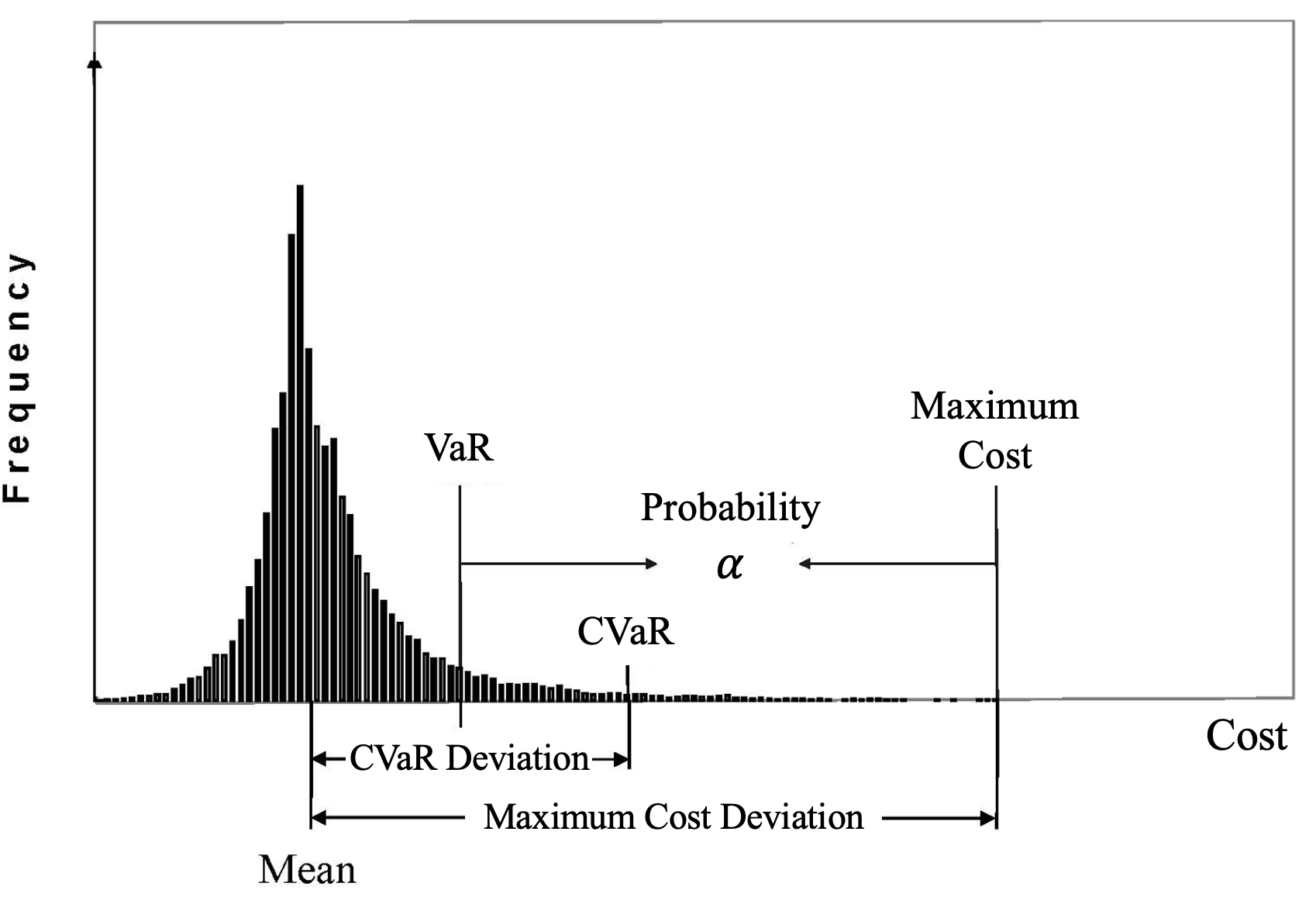
Figure 1: Illustration of CVaR.

2.3 Expected Conditional Risk Measures

We consider a class of multi-period risk function $\mathbb{F}$ mapping from $\mathcal{Z}_{1,\infty}:=\mathcal{Z}_{1}\times\mathcal{Z}_{2}\times\cdots\times\mathcal{Z}_{t}\times\cdots$ to $\mathbb{R}$ as follows:

$$\mathbb{F}(c_{[1,\infty]}|s_{1})= c_{1}+\gamma\rho^{s_{1}}_{2}(c_{2})+\lim_{T\to\infty}\sum_{t=3}^{T}\gamma^{t-1}\mathbb{E}_{s_{[1,t-1]}}\left[{\rho_{t}^{s_{[1,t-1]}}}(c_{t})\right],$$ (3)

where ${\rho_{t}^{s_{[1,t-1]}}}$ is the coherent one-step conditional risk measure mapping from $\mathcal{Z}_{t}$ to $\mathcal{Z}_{t-1}$ defined in Eq. (1) to represent the risk given the information available up to (including) stage $t-1$, and the expectation is taken with respect to the random history $s_{[1,t-1]}$. This class of multi-period risk measures is called expected conditional risk measures (ECRMs), first introduced in Homem-de Mello & Pagnoncelli (2016).

Using the specific risk measure defined in (1) and (2) and applying tower property of expectations on (3), we have

$$\min_{a_{[1,\infty]}}\mathbb{F}(c_{[1,\infty]}|s_{1})$$

$$= \min_{a_{1},\eta_{2}}\Big{\{}C(s_{1},a_{1})+\gamma\lambda\eta_{2}+\gamma\mathbb{E}^{s_{1}}_{s_{2}}\Big{[}\min_{a_{2},\eta_{3}}\Big{\{}\frac{\lambda}{\alpha}[C(s_{2},a_{2})-\eta_{2}]_{+}$$

$$+(1-\lambda)C(s_{2},a_{2})+\gamma\lambda\eta_{3}+\gamma\mathbb{E}^{s_{2}}_{s_{3}}\Big{[}\min_{a_{3},\eta_{4}}\Big{\{}\frac{\lambda}{\alpha}[C(s_{3},a_{3})-\eta_{3}]_{+}$$

$$+(1-\lambda)C(s_{3},a_{3})+\gamma\lambda\eta_{4}+\cdots\Big{\}}\Big{]}\Big{\}}\Big{]}\Big{\}},$$ (4)

where $\mathbb{E}_{s_{t}}^{s_{t-1}}=\mathbb{E}_{s_{t}}[\cdot|{s_{t-1}}]$ is the conditional expectation and we apply the Markov property to recast $\mathbb{E}_{s_{t}}^{s_{[1,t-1]}}$ as $\mathbb{E}_{s_{t}}^{s_{t-1}}$. The auxiliary variable $\eta_{t}$ from Eq. (2) is decided before taking conditional expectation $\mathbb{E}^{s_{t-1}}_{s_{t}}$ and thus it can be regarded as a $(t-1)$-stage action, similar to $a_{t-1}$. Here, $\eta_{t}$ denotes the tail information of state $s_{t}$’s immediate cost (i.e., $\eta_{t}^{*}=\text{VaR}_{\alpha}[C(s_{t},a_{t})|s_{[1,t-1]}]$), which helps us take risk into account when making decisions. We refer interested readers to Yu & Shen (2022) for discussions on the time-consistency of ECRMs and contraction property of the corresponding risk-averse Bellman equation.

Based on formulation (4), we observe that the key differences between (4) and risk-neutral RL are (i) the augmentation of the action space $a_{t}\in\mathcal{A}$ to be $(a_{t},\eta_{t+1})\in\mathcal{A}\times\mathcal{H}$ for all time steps $t\geq 1$ to help learn the tail information of cost distribution, and (ii) the manipulation on immediate costs, i.e., replacing $C(s_{1},a_{1})$ with $\bar{C}_{1}(s_{1},a_{1},\eta_{2})=C(s_{1},a_{1})+\gamma\lambda\eta_{2}$ and replacing $C(s_{t},a_{t})$ with $\bar{C}_{t}(s_{t},\eta_{t},a_{t},\eta_{t+1})=\frac{\lambda}{\alpha}[C(s_{t},a_{t})-\eta_{t}]_{+}+(1-\lambda)C(s_{t},a_{t})+\gamma\lambda\eta_{t+1}$ for $t\geq 2$. Note that for time steps $t\geq 2$, the calculations of immediate costs $\bar{C}_{t}(s_{t},\eta_{t},a_{t},\eta_{t+1})$ involve both the action $\eta_{t}$ from the previous time step $t-1$ and $\eta_{t+1}$ from the current time step $t$. As a result, we augment the state space $s_{t}\in\mathcal{S}$ to be $(s_{t},\eta_{t})\in\mathcal{S}\times\mathcal{H}$ for all $t\geq 2$, where $\eta_{t}$ is the previous action taken in time step $t-1$. To discretize the space $\mathcal{H}=[0,1]$, we assume that $\eta_{t}$ has $H+1$ possible values in total and the $h$-th element of the $\mathcal{H}$-space is $\frac{h}{H}$ for all $h=0,1,\ldots,H$. This leads to the following proposition.

Proposition 1.

Define the augmented action space as $\bar{\mathcal{A}}=\mathcal{A}\times\mathcal{H}$, augmented state space as $\bar{\mathcal{S}}=\mathcal{S}\times\mathcal{H}$, and the state-action transition matrix under policy $\pi$ as $\bar{P}_{(s_{t},\eta_{t},a_{t},\eta_{t+1})\to(s_{t}^{\prime},\eta_{t}^{\prime},a_{t}^{\prime},\eta_{t+1}^{\prime})}=P(s_{t}^{\prime}|s_{t},a_{t})\pi(a_{t}^{\prime},\eta_{t+1}^{\prime}|s_{t}^{\prime},\eta_{t}^{\prime})$, if $\eta_{t}^{\prime}=\eta_{t+1}$; otherwise, $\bar{P}_{(s_{t},\eta_{t},a_{t},\eta_{t+1})\to(s_{t}^{\prime},\eta_{t}^{\prime},a_{t}^{\prime},\eta_{t+1}^{\prime})}=0$. Then the risk-averse RL with ECRM-based objective function (4) is equivalent to a risk-neutral RL with $\bar{M}=(\bar{\mathcal{S}},\bar{\mathcal{A}},\bar{C},\bar{P},\gamma,\rho)$.

The proof of Proposition 1 is straightforward and omitted here. Note that although the risk-averse RL with ECRM can be reformulated as a risk-neutral RL, the modified immediate cost $\bar{C}_{1}(s_{1},a_{1},\eta_{2})$ in the first time step has a different form than $\bar{C}_{t}(s_{t},\eta_{t},a_{t},\eta_{t+1})$ in other time steps $t\geq 2$. Due to this, the conventional Bellman equation used in risk-neutral RL is not applicable here, thereby preventing us from directly employing the results of the risk-neutral policy gradient algorithms.

3 Global Optimality and Convergence of Risk-Averse Policy Gradient Methods

According to formulation (4), we should distinguish the value functions and policies for ECRMs-based objectives between the first time step and others because of the differences in the immediate costs. Furthermore, starting from time step 2, problem (4) reduces to a risk-neutral RL with the same form of manipulated costs $\bar{C}_{t}(s_{t},\eta_{t},a_{t},\eta_{t+1})$ for time steps $t\geq 2$, and according to Puterman (2014), there exists a deterministic stationary Markov optimal policy. As a result, we consider a class of policies $\pi^{\theta}=(\pi_{1}^{\theta_{1}},\pi_{2}^{\theta_{2}})\in\Delta(\mathcal{A}\times\mathcal{H})^{|\mathcal{S}|+|\mathcal{S}||\mathcal{H}|}$ where $\pi_{1}^{\theta_{1}}(a_{1},\eta_{2}|s_{1})$ is the policy for the first time step parameterized by $\theta_{1}$ and $\pi_{2}^{\theta_{2}}(a_{t},\eta_{t+1}|s_{t},\eta_{t}),\ \forall t\geq 2$ is the stationary policy for the following time steps parameterized by $\theta_{2}$. We omit the dependence of $\pi$ on $\theta$ in the following for ease of presentation. The goal is to solve the optimization problem below

$$\min_{\pi\in{\Delta}(\mathcal{A}\times\mathcal{H})^{|\mathcal{S}|+|\mathcal{S}||\mathcal{H}|}}J^{\pi}(\rho)$$ (5)

where we denote $\pi^{*}$ as the optimal policy and $J^{*}(\rho)$ as the optimal objective value. The value and action-value functions for the first time step are defined as

$$J^{\pi}(\rho)= \mathbb{E}_{s_{1}\sim\rho}[J^{\pi}(s_{1})]$$

$$= \mathbb{E}_{s_{1}\sim\rho}\mathbb{E}_{(a_{1},\eta_{2})\sim\pi_{1}(\cdot,\cdot|s_{1})}[Q^{\pi_{2}}(s_{1},a_{1},\eta_{2})]$$ (6)

and

$$Q^{\pi_{2}}(s_{1},a_{1},\eta_{2})=C(s_{1},a_{1})+\gamma\lambda\eta_{2}+\gamma\mathbb{E}^{s_{1},a_{1}}_{s_{2}}\mathbb{E}_{(a_{2},\eta_{3})\sim\pi_{2}(\cdot,\cdot|s_{2},\eta_{2})}\Big{[}\Big{\{}\frac{\lambda}{\alpha}[C(s_{2},a_{2})-\eta_{2}]_{+}$$

$$+(1-\lambda)C(s_{2},a_{2})+\gamma\lambda\eta_{3}+\gamma\mathbb{E}^{s_{2},a_{2}}_{s_{3}}\mathbb{E}_{(a_{3},\eta_{4})\sim\pi_{2}(\cdot,\cdot|s_{3},\eta_{3})}\Big{[}\Big{\{}\frac{\lambda}{\alpha}[C(s_{3},a_{3})-\eta_{3}]_{+}$$

$$+(1-\lambda)C(s_{3},a_{3})+\gamma\lambda\eta_{4}+\cdots\Big{\}}\Big{]}\Big{\}}\Big{]},$$

respectively. Correspondingly, we define value functions for time steps $t\geq 2$ with state $(s_{t},\eta_{t})$ as

$$\hat{J}^{\pi_{2}}(s_{t},\eta_{t})=\mathbb{E}_{(a_{t},\eta_{t+1})\sim\pi_{2}(\cdot,\cdot|s_{t},\eta_{t})}[\hat{Q}^{\pi_{2}}(s_{t},\eta_{t},a_{t},\eta_{t+1})]$$

where

$$\hat{Q}^{\pi_{2}}(s_{t},\eta_{t},a_{t},\eta_{t+1})=\frac{\lambda}{\alpha}[C(s_{t},a_{t})-\eta_{t}]_{+}+(1-\lambda)C(s_{t},a_{t})+\gamma\lambda\eta_{t+1}$$

$$+\gamma\mathbb{E}^{s_{t},a_{t}}_{s_{t+1}}\mathbb{E}_{(a_{t+1},\eta_{t+2})\sim\pi_{2}}\Big{[}\Big{\{}\frac{\lambda}{\alpha}[C(s_{t+1},a_{t+1})-\eta_{t+1}]_{+}+(1-\lambda)C(s_{t+1},a_{t+1})+\gamma\lambda\eta_{t+2}+\cdots\Big{\}}\Big{]}$$

$$=\frac{\lambda}{\alpha}[C(s_{t},a_{t})-\eta_{t}]_{+}+(1-\lambda)C(s_{t},a_{t})+\gamma\lambda\eta_{t+1}+\gamma\mathbb{E}^{s_{t},a_{t}}_{s_{t+1}}[\hat{J}^{\pi_{2}}(s_{t+1},\eta_{t+1})].$$ (7)

As a result, we have the following equation:

$$Q^{\pi_{2}}(s_{1},a_{1},\eta_{2})=C(s_{1},a_{1})+\gamma\lambda\eta_{2}+\gamma\mathbb{E}^{s_{1},a_{1}}_{s_{2}}[\hat{J}^{\pi_{2}}(s_{2},\eta_{2})].$$ (8)

We also define advantage functions $A^{\pi}:\mathcal{S}\times\mathcal{A}\times\mathcal{H}\to\mathbb{R}$ for the first time step and $\hat{A}^{\pi_{2}}:\mathcal{S}\times\mathcal{H}\times\mathcal{A}\times\mathcal{H}\to\mathbb{R}$ for time steps $t\geq 2$ as

$$A^{\pi}(s_{1},a_{1},\eta_{2})=J^{\pi}(s_{1})-Q^{\pi_{2}}(s_{1},a_{1},\eta_{2})$$

$$\hat{A}^{\pi_{2}}(s_{t},\eta_{t},a_{t},\eta_{t+1})=\hat{J}^{\pi_{2}}(s_{t},\eta_{t})-\hat{Q}^{\pi_{2}}(s_{t},\eta_{t},a_{t},\eta_{t+1}),$$

respectively. Note that because of the differences between the first time step and others, we cannot directly apply the risk-neutral policy gradient updates and their convergence results. Instead, we need to derive risk-averse policy gradients, i.e., $\nabla_{\theta}J^{\pi}(\rho)=(\nabla_{\theta_{1}}J^{\pi}(\rho),\nabla_{\theta_{2}}J^{\pi}(\rho))$, and use this joint gradient vector to provide convergence guarantees.

Next, we first derive a performance difference lemma in Lemma 1 and the policy gradients for ECRM-based objective functions in Theorem 1, which are applicable to any parameterizations. The proofs are presented in Appendix A.

Lemma 1.

Let $\text{Pr}^{\pi}(\tau|s_{1}=s)$ denote the probability of observing a trajectory $\tau$ when starting in state $s$ and following policy $\pi$. For all policies $\pi,\pi^{\prime}$ and states $s_{1}$,

$$J^{\pi}(s_{1})-J^{\pi^{\prime}}(s_{1})=\mathbb{E}_{\tau\sim\text{Pr}^{\pi^{\prime}}(\tau|s_{1})}\Big{[}A^{\pi}(s_{1},a_{1},\eta_{2})+\sum_{t=2}^{\infty}\gamma^{t-1}\hat{A}^{\pi_{2}}(s_{t},\eta_{t},a_{t},\eta_{t+1})\Big{]}.$$

Let $\text{Pr}^{\pi}(s_{t+1}=s,\eta_{t+1}=\eta|s_{t},\eta_{t})=\sum_{a_{t}}\pi_{2}(a_{t},\eta|s_{t},\eta_{t})P(s|s_{t},a_{t})$ denote the probability that $s_{t+1}=s,\eta_{t+1}=\eta$ when starting in state $s_{t},\eta_{t}$ and following policy $\pi$ and let $d_{s_{2},\eta_{2}}^{\pi}(s,\eta)=(1-\gamma)\sum_{t=0}^{\infty}\gamma^{t}\text{Pr}^{\pi}(s_{t+2}=s,\eta_{t+2}=\eta|s_{2},\eta_{2})$ denote the discounted state visitation distribution starting from state $s_{2},\eta_{2}$. We present the policy gradients of ECRMs-based objective function (5) in the next theorem.

Theorem 1.

The policy gradients of (5) take the following forms

$$\nabla_{\theta_{1}}J^{\pi}(\rho)= \mathbb{E}_{s_{1}\sim\rho}\mathbb{E}_{(a_{1},\eta_{2})\sim\pi_{1}(\cdot|s_{1})}[\nabla_{\theta_{1}}\log\pi_{1}(a_{1},\eta_{2}|s_{1})Q^{\pi_{2}}(s_{1},a_{1},\eta_{2})]$$

$$\nabla_{\theta_{2}}J^{\pi}(\rho)= \frac{\gamma}{1-\gamma}\mathbb{E}_{(s_{t},\eta_{t})\sim d^{\pi}_{\rho^{\pi}}}\mathbb{E}_{(a_{t},\eta_{t+1})\sim\pi_{2}(\cdot|s_{t},\eta_{t})}[\nabla_{\theta_{2}}\log\pi_{2}(a_{t},\eta_{t+1}|s_{t},\eta_{t})\hat{Q}^{\pi_{2}}(s_{t},\eta_{t},a_{t},\eta_{t+1})]$$

where $\rho^{\pi}(s,\eta)=\sum_{s_{1}}\rho(s_{1})\text{Pr}^{\pi_{1}}(s_{2}=s,\eta_{2}=\eta|s_{1})$.

The differences between risk-averse ECRM-based and risk-neutral policy gradients are twofold. First, we break the policy parameters into two parts, $\theta_{1}$ and $\theta_{2}$, and derive the gradient for each one separately. Second, as reflected in the state visitation distribution $d^{\pi}_{\rho^{\pi}}$ in $\nabla_{\theta_{2}}J^{\pi}(\rho)$, the initial state becomes $(s_{2},\eta_{2})$ with initial distribution $\rho^{\pi}(s,\eta)$, different from the risk-neutral gradients where the initial state is $s_{1}$ with distribution $\rho$ and the state visitation distribution is $d_{\rho}^{\pi}$.

Next, we consider two types of parameterizations: (i) constrained direct parameterization in Section 3.1 and (ii) unconstrained softmax parameterization in Section 3.2. Both parameterizations are complete in the sense that any stochastic policy can be represented in the class, and for each of them, we provide global convergence of the risk-averse policy gradient methods with iteration complexities.

3.1 Constrained Direct Parameterization

For direct parameterization, the policies are $\pi_{1}(a_{1},\eta_{2}|s_{1})=\theta_{1}(s_{1},a_{1},\eta_{2})$ and $\pi_{2}(a_{t},\eta_{t+1}|s_{t},\eta_{t})=\theta_{2}(s_{t},\eta_{t},a_{t},\eta_{t+1}),\ \forall t\geq 2$, where $\theta_{1}\in{\Delta}(\mathcal{A}\times\mathcal{H})^{|\mathcal{S}|}$ and $\theta_{2}\in{\Delta}(\mathcal{A}\times\mathcal{H})^{|\mathcal{S}||\mathcal{H}|}$. In this section, we may write $\nabla_{\pi}J^{\pi}(\rho)$ instead of $\nabla_{\theta}J^{\pi^{\theta}}(\rho)$, and the gradients are

$$\frac{\partial J^{\pi}(\rho)}{\partial\pi_{1}(a,\eta|s)}=\rho(s)Q^{\pi_{2}}(s,a,\eta)$$ (9)

$$\frac{\partial J^{\pi}(\rho)}{\partial\pi_{2}(a,\eta^{\prime}|s,\eta)}=\frac{\gamma}{1-\gamma}d_{\rho^{\pi}}^{\pi}(s,\eta)\hat{Q}^{\pi_{2}}(s,\eta,a,\eta^{\prime})$$ (10)

using Theorem 1. Next, we show that the objective function $J^{\pi}(s_{1})$ is smooth. From standard optimization results (see Appendix E), for a smooth function, a small gradient descent update will guarantee to improve the objective value. The omitted proofs of this section are provided in Appendix B.

Lemma 2.

For all starting states $s_{1}$, $J^{\pi}(s_{1})$ is $\frac{2\gamma|\mathcal{A}||\mathcal{H}|}{(1-\gamma)^{3}}||\bar{c}||_{\infty}$-smooth in $\pi$, i.e.,

$$||\nabla_{\pi}J^{\pi}(s_{1})-\nabla_{\pi}J^{\pi^{\prime}}(s_{1})||_{2}\leq\frac{2\gamma|\mathcal{A}||\mathcal{H}|}{(1-\gamma)^{3}}||\bar{c}||_{\infty}||\pi-\pi^{\prime}||_{2},$$

where $||\bar{c}||_{\infty}=\frac{\lambda}{\alpha}+(1-\lambda)+\gamma\lambda$.

However, smoothness alone can only guarantee the convergence of the gradient descent method to a stationary point (i.e., $\nabla_{\pi}J^{\pi}(s_{1})=0$). For non-convex objective functions, in order to ensure convergence to global minima, we need to establish that the gradient of the objective at any parameter dominates the sub-optimality of the parameter, such as Polyak-like gradient domination conditions Polyak (1963). We give a formal definition of gradient domination below.

Definition 2.

Bhandari & Russo (2019) We say $f$ is $(\nu,\mu)$-gradient dominated over $\Theta$ if there exists constants $\nu>0$ and $\mu\geq 0$ such that for all $\theta\in\Theta$,

$$\min_{\theta^{\prime}\in\Theta}f(\theta^{\prime})\geq f(\theta)+\min_{\theta^{\prime}\in\Theta}\left[\nu\langle\nabla f(\theta),\theta^{\prime}-\theta\rangle+\frac{\mu}{2}||\theta-\theta^{\prime}||_{2}^{2}\right].$$

The function is said to be gradient dominated with degree one if $\mu=0$ and with degree two if $\mu>0$.

Any stationary point of a gradient-dominated function is globally optimal. To see this, we note that for any stationary point $\theta$, we have $\langle\nabla f(\theta),\theta^{\prime}-\theta\rangle\geq 0$ for all $\theta^{\prime}\in\Theta$. Then the minimizer of the right-hand side in Definition 2 is $\theta$, implying $\min_{\theta^{\prime}\in\Theta}f(\theta^{\prime})\geq f(\theta)$.

In the next theorem, we show that the value function $J^{\pi}(\rho)$ is gradient dominated with degree one, which will be used to quantify the convergence rate of projected gradient descent methods in Theorem 3 later. Following Agarwal et al. (2021), even though we are interested in the value $J^{\pi}(\rho)$, we will consider the gradient with respect to another state distribution $\mu\in\Delta(\mathcal{S})$, which allows for greater flexibility in our analysis.

Theorem 2.

Let $\pi_{1}^{LB}=\min_{s,a,\eta}\pi_{1}(a,\eta|s)$. For the direct policy parameterization, for all state distributions $\rho,\ \mu\in\Delta(\mathcal{S})$, we have

$$J^{\pi}(\rho)-J^{*}(\rho)\leq D_{1}\max_{\bar{\pi}\in{\Delta}(\mathcal{A}\times\mathcal{H})^{|\mathcal{S}|+|\mathcal{S}||\mathcal{H}|}}(\pi-\bar{\pi})^{\mathsf{T}}\nabla_{\pi}J^{\pi}(\mu)$$

where $D_{1}=\max\{||\frac{\rho}{\mu}||_{\infty},\frac{1}{(1-\gamma)\pi_{1}^{LB}}||\frac{d_{\rho^{\pi^{*}}}^{\pi^{*}}}{\mu^{P}}||_{\infty}\}$ and $\mu^{P}(s,\eta)=\sum_{s_{1},a_{1}}\mu(s_{1})P(s|s_{1},a_{1}),\forall s\in\mathcal{S},\ \eta\in\mathcal{H}$.

Note that the significance of Theorem 2 is that although the gradient is with respect to $J^{\pi}(\mu)$, the final guarantee applies to all distributions $\rho$.

Remark 1.

Compared to Lemma 4 in Agarwal et al. (2021):

$$V^{\pi}(\rho)-V^{*}(\rho)\leq\frac{1}{1-\gamma}||\frac{d_{\rho}^{\pi^{*}}}{\mu}||_{\infty}\max_{\bar{\pi}}(\pi-\bar{\pi})^{\mathsf{T}}\nabla_{\pi}V^{\pi}(\mu),$$

in risk-neutral policy gradient methods, some conditions on the state distribution of $\pi$, or equivalently $\mu$, are necessary for stationarity to imply optimality as illustrated in Section 4.3 of Agarwal et al. (2021). For example, if the starting state distribution is not strictly positive, i.e., $\mu(s_{1})=0$ for some state $s_{1}$, then the coefficient $||\frac{d_{\rho}^{\pi^{*}}}{\mu}||_{\infty}=+\infty$.

Similarly, in risk-averse policy gradient methods, according to our Theorem 2, we not only need a strictly positive distribution $\mu$ for the starting state $s_{1}$, but also need a strictly positive distribution $\mu^{\pi}$ for second-step states $s_{2},\eta_{2}$. To achieve this, we need to ensure that (i) each possible value of $\eta_{2}$ is achieved with a positive probability (i.e., $\pi_{1}^{LB}>0$), and (ii) each possible value of $s_{2}$ is reachable from the initial distribution $\mu$ (i.e., $\mu^{P}>0$).

With the policy gradient results in Theorem 1, we consider a projected gradient descent method, where we directly update the policy parameter in the gradient descent direction and then project it back onto the simplex if the constraints are violated after a gradient update. The projected gradient descent algorithm updates

$$\pi^{(t+1)}=P_{{\Delta}(\mathcal{A}\times\mathcal{H})^{|\mathcal{S}|+|\mathcal{S}||\mathcal{H}|}}(\pi^{(t)}-\beta\nabla_{\pi}J^{(t)}(\mu))$$

where $P_{{\Delta}(\mathcal{A}\times\mathcal{H})^{|\mathcal{S}|+|\mathcal{S}||\mathcal{H}|}}$ is the projection onto ${\Delta}(\mathcal{A}\times\mathcal{H})^{|\mathcal{S}|+|\mathcal{S}||\mathcal{H}|}$ in the Euclidean norm, and $\beta$ is the step size. Using Theorem 2, we now give an iteration complexity bound for projected gradient descent methods.

Theorem 3.

Let $\pi_{1}^{LB}=\inf_{t\geq 1}\min_{s,a,\eta}\pi_{1}^{(t)}(a,\eta|s)$, $D_{1}=\max\{||\frac{\rho}{\mu}||_{\infty},\frac{1}{(1-\gamma)\pi_{1}^{LB}}||\frac{d_{\rho^{\pi^{*}}}^{\pi^{*}}}{\mu^{P}}||_{\infty}\}$. The projected gradient descent algorithm on $J^{\pi}(\mu)$ with stepsize $\beta=\frac{(1-\gamma)^{3}}{2\gamma|\mathcal{A}||\mathcal{H}|||\bar{c}||_{\infty}}$ satisfies for all distributions $\rho\in\Delta(\mathcal{S})$,

$$\min_{t\leq T}J^{(t)}(\rho)-J^{*}(\rho)\leq\epsilon$$

whenever

$$T\geq D_{1}^{2}\frac{128\gamma|\mathcal{S}||\mathcal{A}||\mathcal{H}|^{2}}{(1-\gamma)^{3}\epsilon^{2}}\bar{C}||\bar{c}||_{\infty}$$

with $\bar{C}=(\frac{\lambda}{\alpha}+\lambda+\frac{1}{1-\gamma}||\bar{c}||_{\infty}),\ ||\bar{c}||_{\infty}=\frac{\lambda}{\alpha}+(1-\lambda)+\gamma\lambda$.

A proof is provided in Appendix B, where we invoke a standard iteration complexity result of projected gradient descent on smooth functions to show that the gradient magnitude with respect to all feasible directions is small. Then, we use Theorem 2 to complete the proof. Note that the guarantee we provide is for the best policy found over $T$ rounds, which is standard in the non-convex optimization literature. As can be seen from Theorems 2 and 3, when $\pi_{1}^{LB}\to 0$, the iteration bound $T\to+\infty$. To circumvent this issue, we consider a softmax parameterization with log barrier regularizer in the next section, which ensures that $\pi_{1}^{LB}>0$.

3.2 Unconstrained Softmax Parameterization

In this section, we aim to solve the optimization problem (5) with the following softmax parameterization: for all $s_{1},a_{1},\eta_{2}$ and $s_{t},\eta_{t},a_{t},\eta_{t+1},\ t\geq 2$, we have

$$\pi_{1}^{\theta}(a_{1},\eta_{2}|s_{1}) =\frac{\exp{(\theta_{1}(s_{1},a_{1},\eta_{2})})}{\sum_{a_{1}^{\prime},\eta_{2}^{\prime}}\exp{(\theta_{1}(s_{1},a_{1}^{\prime},\eta_{2}^{\prime})})},$$

$$\pi_{2}^{\theta}(a_{t},\eta_{t+1}|s_{t},\eta_{t}) =\frac{\exp{(\theta_{2}(s_{t},\eta_{t},a_{t},\eta_{t+1})})}{\sum_{a_{t}^{\prime},\eta_{t+1}^{\prime}}\exp{(\theta_{2}(s_{t},\eta_{t},a_{t}^{\prime},\eta_{t+1}^{\prime})})}.$$

Note that the softmax parameterization is preferable to the direct parameterization, since the parameters $\theta$ are unconstrained (i.e., $\pi_{1}^{\theta},\pi_{2}^{\theta}$ belong to the probability simplex automatically) and standard unconstrained optimization algorithms can be employed. The omitted proofs of this section are provided in Appendix C.

Lemma 3.

Using the softmax parameterization, the gradients take the following forms:

$$\frac{\partial J^{\pi^{\theta}}(\mu)}{\partial\theta_{1}(s_{1},a_{1},\eta_{2})}=\mu(s_{1})\pi_{1}^{\theta}(a_{1},\eta_{2}|s_{1})(-A^{\pi^{\theta}}(s_{1},a_{1},\eta_{2}))$$

$$\frac{\partial J^{\pi^{\theta}}(\mu)}{\partial\theta_{2}(s_{t},\eta_{t},a_{t},\eta_{t+1})}=\frac{\gamma}{1-\gamma}d_{\mu^{\pi}}^{\pi}(s_{t},\eta_{t})\pi_{2}^{\theta}(a_{t},\eta_{t+1}|s_{t},\eta_{t})(-\hat{A}^{\pi_{2}^{\theta}}(s_{t},\eta_{t},a_{t},\eta_{t+1})).$$

Because the action probabilities depend exponentially on the parameters $\theta$, policies can quickly become near deterministic and lack exploration, leading to slow convergence. In this section, we add an entropy-based regularization term to the objective function to keep the probabilities from getting too small. Recall that the relative-entropy for distributions $p$ and $q$ is defined as $\text{KL}(p,q):=\mathbb{E}_{x\sim p}[-\log q(x)/p(x)]$. Denote the uniform distribution over set $\mathcal{X}$ as $\text{Unif}_{\mathcal{X}}$, and consider the following log barrier regularized objective:

$$L_{\kappa}(\theta):= J^{\pi^{\theta}}(\mu)+\kappa\mathbb{E}_{s_{1}\sim\text{Unif}_{\mathcal{S}}}[\text{KL}(\text{Unif}_{\mathcal{A}\times\mathcal{H}},\pi_{1}^{\theta}(\cdot,\cdot|s_{1})]+\kappa\mathbb{E}_{s_{t},\eta_{t}\sim\text{Unif}_{\mathcal{S}\times\mathcal{H}}}[\text{KL}(\text{Unif}_{\mathcal{A}\times\mathcal{H}},\pi_{2}^{\theta}(\cdot,\cdot|s_{t},\eta_{t})]$$

$$= J^{\pi^{\theta}}(\mu)-\frac{\kappa}{|\mathcal{S}||\mathcal{A}||\mathcal{H}|}\sum_{s_{1},a_{1},\eta_{2}}\log\pi_{1}^{\theta}(a_{1},\eta_{2}|s_{1})-\frac{\kappa}{|\mathcal{S}||\mathcal{H}||\mathcal{A}||\mathcal{H}|}\sum_{s_{t},\eta_{t},a_{t},\eta_{t+1}}\log\pi_{2}^{\theta}(a_{t},\eta_{t+1}|s_{t},\eta_{t})$$

$$-2\kappa\log|\mathcal{A}||\mathcal{H}|,$$

where $\kappa>0$ is a regularization parameter and the last (constant) term is not relevant to optimization. We first show that $L_{\kappa}(\theta)$ is smooth in the next lemma.

Lemma 4.

The log barrier regularized objective function $L_{\kappa}(\theta)$ is $\sigma_{\kappa}$-smooth with $\sigma_{\kappa}=6(\frac{\lambda}{\alpha}+\lambda)+\frac{8}{(1-\gamma)^{3}}||\bar{c}||_{\infty}+\frac{2\kappa}{|\mathcal{S}|}+\frac{2\kappa}{|\mathcal{S}||\mathcal{H}|}$.

Our next theorem shows that the approximate first-order stationary points of $L_{\kappa}(\theta)$ are approximately globally optimal with respect to $J^{\pi}(\rho)$, as long as the regularization parameter $\kappa$ is small enough.

Theorem 4.

Let $\pi_{1}^{LB}=\min_{s,a,\eta}\pi_{1}^{\theta}(a,\eta|s)$. Suppose

$$||\nabla_{\theta_{1}}L_{\kappa}(\theta)||_{2}\leq\epsilon_{1}\leq\frac{\kappa}{2|\mathcal{S}||\mathcal{A}||\mathcal{H}|},$$

$$||\nabla_{\theta_{2}}L_{\kappa}(\theta)||_{2}\leq\epsilon_{2}\leq\frac{\kappa}{2|\mathcal{S}||\mathcal{H}||\mathcal{A}||\mathcal{H}|},$$

then we have that for all starting state distributions $\rho$:

$$J^{\pi^{\theta}}(\rho)-J^{*}(\rho)\leq 2\kappa||\frac{\rho}{\mu}||_{\infty}+\frac{2\kappa}{(1-\gamma)\pi_{1}^{LB}}||\frac{d_{\rho^{\pi^{*}}}^{\pi^{*}}}{\mu^{P}}||_{\infty}.$$

Now consider policy gradient descent updates for $L_{\kappa}(\theta)$ as follows:

$$\theta^{(t+1)}:=\theta^{(t)}-\beta\nabla_{\theta}L_{\kappa}(\theta^{(t)}).$$ (11)

Lemma 5.

Using the policy gradient updates (11) for $L_{\kappa}(\theta)$ with $\beta=\frac{1}{\sigma_{\kappa}}$, we have $\pi_{1}^{LB}:=\inf_{t\geq 1}\min_{s,a,\eta}\pi_{1}^{\theta^{(t)}}(a,\eta|s)>0$ and $\pi_{2}^{LB}:=\inf_{t\geq 1}\min_{s,a,\eta,\eta^{\prime}}\pi_{2}^{\theta^{(t)}}(a,\eta^{\prime}|s,\eta)>0$.

Using Theorem 4, Lemma 5 and standard results on the convergence of gradient descent, we obtain the following iteration complexity for softmax parameterization with log barrier regularization.

Theorem 5.

Let $\sigma_{\kappa}=6(\frac{\lambda}{\alpha}+\lambda)+\frac{8}{(1-\gamma)^{3}}||\bar{c}||_{\infty}+\frac{2\kappa}{|\mathcal{S}|}+\frac{2\kappa}{|\mathcal{S}||\mathcal{H}|}$ and $D_{2}=||\frac{\rho}{\mu}||_{\infty}+\frac{1}{(1-\gamma)\pi_{1}^{LB}}||\frac{d_{\rho^{\pi^{*}}}^{\pi^{*}}}{\mu^{P}}||_{\infty}$. Starting from any initial finite-value $\theta^{(0)}$, consider the updates (11) with $\kappa=\frac{\epsilon}{2D_{2}}$ and $\beta=\frac{1}{\sigma_{\kappa}}$. Then for all starting state distributions $\rho$, we have

$$\min_{t\leq T}J^{(t)}(\rho)-J^{*}(\rho)\leq\epsilon$$

whenever

$$T\geq\frac{64(3(\frac{\lambda}{\alpha}+\lambda)+4||\bar{c}||_{\infty}+2)\bar{B}|\mathcal{S}|^{2}|\mathcal{A}|^{2}|\mathcal{H}|^{4}}{(1-\gamma)^{3}\epsilon^{2}}D_{2}^{2}$$

with $\bar{B}=\bar{C}-\log\pi_{1}^{LB}-\log\pi_{2}^{LB}$.

4 Numerical Results

In this section, we propose a risk-averse REINFORCE algorithm for handling discrete state and action space in Section 4.1 and a risk-averse actor-critic algorithm for handling continuous state and action space in Section 4.2, respectively.

4.1 Algorithms for Discrete State and Action Space

We first propose a risk-averse REINFORCE algorithm Williams (1992) in Algorithm 1 with softmax parameterization, which works for discrete state and action space.

Algorithm 1 Risk-averse REINFORCE with softmax parameterization

1:  Initialize $\theta_{1}(s_{1},a_{1},\eta_{2}),\ \forall s_{1}\in\mathcal{S},\ a_{1}\in\mathcal{A},\ \eta_{2}\in\mathcal{H}$ and set softmax policy $\pi_{1}^{\theta}(a_{1},\eta_{2}|s_{1})=\frac{\exp{(\theta_{1}(s_{1},a_{1},\eta_{2})})}{\sum_{a_{1}^{\prime},\eta_{2}^{\prime}}\exp{(\theta_{1}(s_{1},a_{1}^{\prime},\eta_{2}^{\prime})})}$.

2:  Initialize $\theta_{2}(s_{t},\eta_{t},a_{t},\eta_{t+1}),\ \forall s_{t}\in\mathcal{S},\ a_{t}\in\mathcal{A},\ \eta_{t},\ \eta_{t+1}\in\mathcal{H}$ and set softmax policy $\pi_{2}^{\theta}(a_{t},\eta_{t+1}|s_{t},\eta_{t})=\frac{\exp{(\theta_{2}(s_{t},\eta_{t},a_{t},\eta_{t+1})})}{\sum_{a_{t}^{\prime},\eta_{t+1}^{\prime}}\exp{(\theta_{2}(s_{t},\eta_{t},a_{t}^{\prime},\eta_{t+1}^{\prime})})}$.

3:  while not converged do

4:    Generate one trajectory on policy $\pi^{\theta}=(\pi_{1}^{\theta},\pi_{2}^{\theta})$: $s_{1},a_{1},\eta_{2},c_{1},s_{2},\ldots,s_{T-1},a_{T-1},\eta_{T},c_{T-1},s_{T}$.

5:    Modify immediate costs as $\bar{c}_{1}=c_{1}+\gamma\lambda\eta_{2},\ \bar{c}_{t}=\frac{\lambda}{\alpha}[c_{t}-\eta_{t}]_{+}+(1-\lambda)c_{t}+\gamma\lambda\eta_{t+1},\ \forall t\geq 2$.

6:    Update $\theta_{1}:=\theta_{1}-\beta\nabla_{\theta_{1}}\log\pi_{1}^{\theta}(a_{1},\eta_{2}|s_{1})\sum_{\tau=1}^{T-1}\gamma^{\tau-1}\bar{c}_{\tau}$.

7:    Update $\theta_{2}:=\theta_{2}-\beta\sum_{t=2}^{T-1}\nabla_{\theta_{2}}\log\pi_{2}^{\theta}(a_{t},\eta_{t+1}|s_{t},\eta_{t})\sum_{\tau=t}^{T-1}\gamma^{\tau-t}\bar{c}_{\tau}$.

8:  end while

We implement Algorithm 1 on a stochastic version of the $4\times 4$ Cliffwalk environment Sutton & Barto (2018) (see Figure 2), where the agent needs to travel from a start ($[3,0]$) to a goal state ($[3,3]$) while incurring as little cost as possible. Each action incurs 1 cost, but the shortest path lies next to a cliff ($[3,1]$ and $[3,2]$), where entering the cliff corresponds to a cost of 5 and the agent will return to the start. Because the classical Cliffwalk environment is deterministic, we consider a stochastic variant following Huang et al. (2021), where the row of cells above the cliff ($[2,1]$ and $[2,2]$) are slippery, and entering these slippery cells induces a transition into the cliff with probability $p=0.1$. The discount factor $\gamma$ is set to 0.98, and the confidence level for CVaR is set to $\alpha=0.05$. Because each immediate cost can only take values 1 or 5, we set the $\eta$-space as $\mathcal{H}=\{1,5\}$. For this stochastic environment, the shortest path is the blue path in Figure 2, which takes a cost of 5 if not entering the cliff; however, a safer path is the orange path, which induces a deterministic cost of 7.

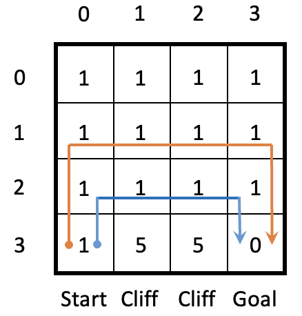
Figure 2: A $4\times 4$ stochastic Cliffwalk environment.

We train the model over 10000 episodes where each episode starts at a random state and continues until the goal state is reached or the maximum time step (i.e., 500) is reached. All the hyperparameters are kept the same across different trials, except for the risk parameters $\lambda$ which is swept across 0, 0.25, 0.5, 0.75, 1. For each of these values, we perform the task over 10 independent simulation runs. The average test costs (when we start at state $[3,0]$ and choose the action having the largest probability) in the first 3000 episodes over the 10 simulation runs are recorded in Figure 3(a), where the colored shades represent the standard deviation. To present a detailed description of these cost profiles, we also look at a specific run and plot the test cost in the last 1000 episodes in Figure 3(b).

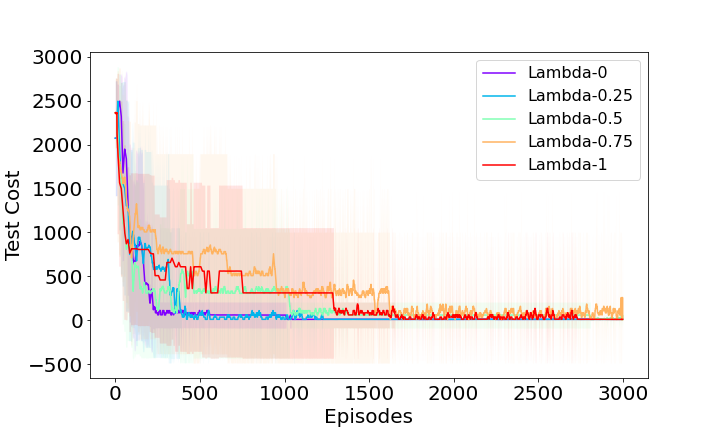
(a) Average test cost over 10 runs with varying $\lambda$.

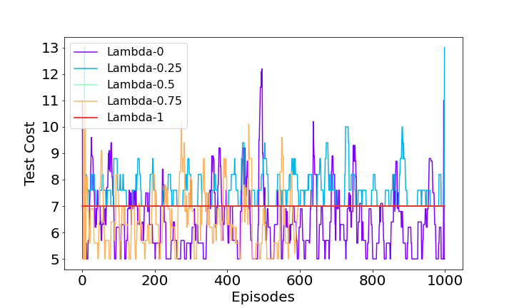
(b) Test cost in the last 1000 episodes in one run with varying $\lambda$.

Figure 3: Test cost over 10 independent runs with varying $\lambda$.

From Figure 3(a), $\lambda=1$ produces the largest variance of test cost in the first 1500 episodes, after which the policy gradually converges to the safer path with a steady cost of 7. When we look at Figure 3(b), $\lambda=0$ converges to the shortest path with the highest variance, and $\lambda=0.25$ chooses a combination of the shortest and safer paths (i.e., move right at state $[2,0]$, move up at state $[2,1]$, and then follow the safer path). On the other hand, $\lambda=0.5,0.75,1$ all converge to the same safer path with a steady cost of 7 in the last 400 episodes, so they overlap in the figure.

Next, we present the average action probabilities ($\pi_{2}^{\theta}(\cdot,\cdot|s_{t},\eta_{t})$ in the last episode) at state $s_{t}=[2,0],\ \eta_{t}=0$ over the 10 independent runs with varying $\lambda$ in Figure 4, where actions $a=0,1,2,3$ represent moving up, right, down and left respectively, and actions $\eta=1,5$ represent the VaR of the next state’s cost distribution. A lighter color denotes a higher probability. From Figure 4, when $\lambda=0,0.25$, the learned optimal action at state $s=[2,0]$ is to move right ($a=1$) with $\eta=5$, as entering state $[2,1]$ will induce a cost of 5 with probability 0.1. As $\lambda$ increases, the optimal action shifts to move up $(a=0)$ with $\eta=1$. We present the average action probabilities at each state in the learned optimal path in Figures 7–11 in Appendix F.

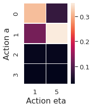
(a) $\lambda=0$

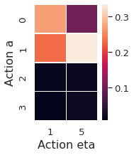
(b) $\lambda=0.25$

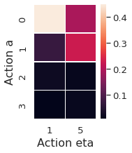
(c) $\lambda=0.5$

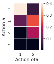
(d) $\lambda=0.75$

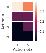
(e) $\lambda=1$

Figure 4: Average action probabilities at state $s_{t}=[2,0],\ \eta_{t}=0$.

Lastly, we display the impact of modifying the regularizer parameter $\kappa$ from 0 to 0.5 in Figure 5. A higher $\kappa$ helps speed up the convergence to a steady path while $\kappa=0$ generates the highest variance of test cost after 2000 episodes.

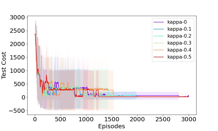
Figure 5: Average test cost over 10 runs with varying $\kappa$.

4.2 Algorithms for Continuous State and Action Space

Our method can be also extended to solve problems with continuous state and action space. To design a risk-averse actor-critic algorithm, we replace the tabular policy $\pi_{1}$ and $\pi_{2}$ in Algorithm 1 with neural networks parameterized by $\theta_{1}$ and $\theta_{2}$, respectively. We also construct neural networks for value critics $v_{1}(s_{1})$ with parameter $w_{1}$ and value critic $v_{2}(s_{t},\eta_{t})$ with parameter $w_{2}$. The main steps for the risk-averse actor-critic are outlined in Algorithm 2.

Algorithm 2 Risk-Averse Actor-Critic

1:  Initialize policy $\pi_{1}(a_{1},\eta_{2}|s_{1})$ with parameter $\theta_{1}$ and policy $\pi_{2}(a_{t},\eta_{t+1}|s_{t},\eta_{t})$ with parameter $\theta_{2}$.

2:  Initialize value critic $v_{1}(s_{1})$ with parameter $w_{1}$ and value critic $v_{2}(s_{t},\eta_{t})$ with parameter $w_{2}$.

3:  while not converged do

4:    Generate one trajectory on policy $\pi^{\theta}=(\pi_{1}^{\theta_{1}},\pi_{2}^{\theta_{2}})$: $s_{1},a_{1},\eta_{2},c_{1},s_{2},\ldots,s_{T-1},a_{T-1},\eta_{T},c_{T-1},s_{T}$.

5:    Modify immediate costs as $\bar{c}_{1}=c_{1}+\gamma\lambda\eta_{2},\ \bar{c}_{t}=\frac{\lambda}{\alpha}[c_{t}-\eta_{t}]_{+}+(1-\lambda)c_{t}+\gamma\lambda\eta_{t+1},\ \forall t\geq 2$.

6:    Compute discounted costs: $V_{t}=\sum_{\tau=t}^{T-1}\gamma^{\tau-t}\bar{c}_{\tau}$ for all $t=1,\ldots,T-1$.

7:    Update $w_{1}$ to minimize $||v_{1}^{w_{1}}(s_{1})-V_{1}||^{2}$ and update $w_{2}$ to minimize $\sum_{t=2}^{T-1}||v_{2}^{w_{2}}(s_{t},\eta_{t})-V_{t}||^{2}$.

8:    Update $\theta_{1}:=\theta_{1}-\beta\nabla_{\theta_{1}}\log\pi_{1}^{\theta_{1}}(a_{1},\eta_{2}|s_{1})V_{1}$.

9:    Update $\theta_{2}:=\theta_{2}-\beta\sum_{t=2}^{T-1}\nabla_{\theta_{2}}\log\pi_{2}^{\theta_{2}}(a_{t},\eta_{t+1}|s_{t},\eta_{t})V_{t}$.

10:  end while

We apply Algorithm 2 on the CartPole environment Barto et al. (1983), where the reward is $+1$ for every step taken and the goal is to keep the pole upright for as long as possible. The average test rewards over 5 simulation runs are displayed in Figure 6, where we vary the risk parameter $\lambda$ from 0 to 1. From Figure 6, $\lambda=1$ outperforms all other configurations by producing the highest reward over time.

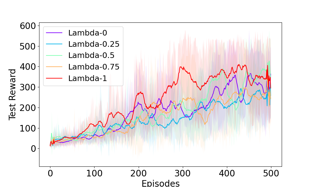
Figure 6: Average test reward over 5 runs with varying $\lambda$.

5 Conclusions

In this paper, we applied a class of dynamic time-consistent coherent risk measures (i.e., ECRMs) on infinite-horizon MDPs and provided global convergence guarantees for risk-averse policy gradient methods under constrained direct parameterization and unconstrained softmax parameterization. Our iteration complexity results closely matched the risk-neutral counterparts in Agarwal et al. (2021).

For future research, it is worth investigating iteration complexities for policy gradient algorithms with restricted policy classes (e.g., log-linear policy and neural policy) and natural policy gradient. It would also be interesting to incorporate distributional RL Bellemare et al. (2017) into this risk-sensitive setting and derive global convergence guarantees.

The appendix is organized as follows.

• Appendix A: proofs of Lemma 1 and Theorem 1.

• Appendix B: proofs in Section 3.1.

• Appendix C: proofs in Section 3.2.

• Appendix D: smoothness proofs.

• Appendix E: standard optimization results.

• Appendix F: additional computational results.

Appendix A Proofs of Lemma 1 and Theorem 1

Proof of Lemma 1.

[Performance difference lemma] Using a telescoping argument, we have

$$J^{\pi}(s_{1})-J^{\pi^{\prime}}(s_{1})= J^{\pi}(s_{1})-\mathbb{E}_{\tau\sim Pr^{\pi^{\prime}}}[\sum_{t=1}^{\infty}\gamma^{t-1}\bar{c}_{t}]$$

$$= J^{\pi}(s_{1})-\mathbb{E}_{\tau\sim Pr^{\pi^{\prime}}}[\sum_{t=1}^{\infty}\gamma^{t-1}(\bar{c}_{t}+J^{\pi}(s_{t})-J^{\pi}(s_{t})]$$

$$\overset{(a)}{=} -\mathbb{E}_{\tau\sim Pr^{\pi^{\prime}}}[\sum_{t=1}^{\infty}\gamma^{t-1}(\bar{c}_{t}+\gamma J^{\pi}(s_{t+1})-J^{\pi}(s_{t})]$$

$$\overset{(b)}{=} -\mathbb{E}_{\tau\sim Pr^{\pi^{\prime}}}[\sum_{t=1}^{\infty}\gamma^{t-1}(\bar{c}_{t}+\gamma\mathbb{E}_{s_{t+1}}^{s_{t},a_{t}}[J^{\pi}(s_{t+1})]-J^{\pi}(s_{t}))],$$

where $(a)$ rearranges terms in the summation and cancels the $J^{\pi}(s_{1})$ term with $J^{\pi}(s_{1})$ outside the summation, and $(b)$ uses the tower property of conditional expectations. For the term $t=1$ inside the summation, we have

$$-\mathbb{E}_{(a_{1},\eta_{2})\sim\pi^{\prime}_{1}(s_{1})}[C(s_{1},a_{1})+\gamma\lambda\eta_{2}+\gamma\mathbb{E}_{s_{2}}^{s_{1},a_{1}}[J^{\pi}(s_{2})]-J^{\pi}(s_{1})]$$

$$= -\mathbb{E}_{(a_{1},\eta_{2})\sim\pi^{\prime}_{1}(s_{1})}[Q^{\pi_{2}}(s_{1},a_{1},\eta_{2})+\gamma\mathbb{E}_{s_{2}}^{s_{1},a_{1}}[J^{\pi}(s_{2})-\hat{J}^{\pi_{2}}(s_{2},\eta_{2})]-J^{\pi}(s_{1})]$$

$$= \mathbb{E}_{(a_{1},\eta_{2})\sim\pi^{\prime}_{1}(s_{1})}[A^{\pi}(s_{1},a_{1},\eta_{2})+\gamma\mathbb{E}_{s_{2}}^{s_{1},a_{1}}[\hat{J}^{\pi_{2}}(s_{2},\eta_{2})-J^{\pi}(s_{2})]]$$ (12)

where the first equality is because of Eq. (8). For terms $t\geq 2$, we have

$$-\mathbb{E}_{\tau\sim Pr^{\pi^{\prime}}}\Big{[}\gamma^{t-1}\Big{(}\frac{\lambda}{\alpha}[C(s_{t},a_{t})-\eta_{t}]_{+}+(1-\lambda)C(s_{t},a_{t})+\gamma\lambda\eta_{t+1}+\gamma\mathbb{E}_{s_{t+1}}^{s_{t},a_{t}}[J^{\pi}(s_{t+1})]-J^{\pi}(s_{t})\Big{)}\Big{]}$$

$$= -\mathbb{E}_{\tau\sim Pr^{\pi^{\prime}}}\Big{[}\gamma^{t-1}\Big{(}\hat{Q}^{\pi_{2}}(s_{t},\eta_{t},a_{t},\eta_{t+1})-\hat{J}^{\pi_{2}}(s_{t},\eta_{t})+\gamma\mathbb{E}_{s_{t+1}}^{s_{t},a_{t}}[J^{\pi}(s_{t+1})-\hat{J}^{\pi_{2}}(s_{t+1},\eta_{t+1})]+(\hat{J}^{\pi_{2}}(s_{t},\eta_{t})-J^{\pi}(s_{t}))\Big{)}\Big{]}$$

$$= \mathbb{E}_{\tau\sim Pr^{\pi^{\prime}}}\Big{[}\gamma^{t-1}\Big{(}\hat{A}^{\pi_{2}}(s_{t},\eta_{t},a_{t},\eta_{t+1})+\gamma\mathbb{E}_{s_{t+1}}^{s_{t},a_{t}}[\hat{J}^{\pi_{2}}(s_{t+1},\eta_{t+1})-J^{\pi}(s_{t+1})]-(\hat{J}^{\pi_{2}}(s_{t},\eta_{t})-J^{\pi}(s_{t}))\Big{)}\Big{]}.$$ (13)

Observing that $\mathbb{E}_{s_{t},a_{t},\eta_{t+1}\sim Pr^{\pi^{\prime}}}\mathbb{E}_{s_{t+1}}^{s_{t},a_{t}}[\hat{J}^{\pi_{2}}(s_{t+1},\eta_{t+1})-J^{\pi}(s_{t+1})]=\mathbb{E}_{s_{t+1},\eta_{t+1}\sim Pr^{\pi^{\prime}}}[\hat{J}^{\pi_{2}}(s_{t+1},\eta_{t+1})-J^{\pi}(s_{t+1})]$ for all $t\geq 1$, the second term in Eq. (12) cancels out the third term in Eq. (13) with $t=2$. Moreover, the second term in Eq. (13) with time step $t$ cancels out the third term in Eq. (13) with time step $t+1$ for all $t\geq 2$. As a result, we have

$$J^{\pi}(s_{1})-J^{\pi^{\prime}}(s_{1})=\mathbb{E}_{\tau\sim\text{Pr}^{\pi^{\prime}}(\tau|s_{1})}\Big{[}A^{\pi}(s_{1},a_{1},\eta_{2})+\sum_{t=2}^{\infty}\gamma^{t-1}\hat{A}^{\pi_{2}}(s_{t},\eta_{t},a_{t},\eta_{t+1})\Big{]}.$$

This completes the proof. ∎

Proof of Theorem 1.

[Risk-averse policy gradients] According to Eq. (6), we have

$$\nabla_{\theta_{1}}J^{\pi}(s_{1}) =\nabla_{\theta_{1}}(\sum_{a_{1},\eta_{2}}\pi_{1}(a_{1},\eta_{2}|s_{1})Q^{\pi_{2}}(s_{1},a_{1},\eta_{2}))$$

$$\overset{(a)}{=}\sum_{a_{1},\eta_{2}}\nabla_{\theta_{1}}\pi_{1}(a_{1},\eta_{2}|s_{1})Q^{\pi_{2}}(s_{1},a_{1},\eta_{2})$$

$$=\mathbb{E}_{(a_{1},\eta_{2})\sim\pi_{1}}[\nabla_{\theta_{1}}\log\pi_{1}(a_{1},\eta_{2}|s_{1})Q^{\pi_{2}}(s_{1},a_{1},\eta_{2})]$$

where $(a)$ is true because $\nabla_{\theta_{1}}Q^{\pi_{2}}(s_{1},a_{1},\eta_{2})=0$. As a result,

$$\nabla_{\theta_{1}}J^{\pi}(\rho) =\nabla_{\theta_{1}}\mathbb{E}_{s_{1}\sim\rho}[J^{\pi}(s_{1})]=\mathbb{E}_{s_{1}\sim\rho}[\nabla_{\theta_{1}}J^{\pi}(s_{1})].$$

Based on the definition of $Q^{\pi_{2}}(s_{1},a_{1},\eta_{2})$, we have

$$\nabla_{\theta_{2}}J^{\pi}(s_{1})= \nabla_{\theta_{2}}(\sum_{a_{1},\eta_{2}}\pi_{1}(a_{1},\eta_{2}|s_{1})Q^{\pi_{2}}(s_{1},a_{1},\eta_{2}))$$

$$= \sum_{a_{1},\eta_{2}}(\pi_{1}(a_{1},\eta_{2}|s_{1})\nabla_{\theta_{2}}(c_{1}+\gamma\lambda\eta_{2}+\gamma\mathbb{E}^{s_{1}}_{s_{2}}[\hat{J}^{\pi_{2}}(s_{2},\eta_{2})]))$$

$$= \gamma\sum_{a_{1},\eta_{2}}\pi_{1}(a_{1},\eta_{2}|s_{1})\sum_{s_{2}}P(s_{2}|s_{1},a_{1})\nabla_{\theta_{2}}\hat{J}^{\pi_{2}}(s_{2},\eta_{2})$$

$$= \gamma\sum_{s_{2},\eta_{2}}\text{Pr}^{\pi_{1}}(s_{2},\eta_{2}|s_{1})\nabla_{\theta_{2}}\hat{J}^{\pi_{2}}(s_{2},\eta_{2})$$

Now for $\nabla_{\theta_{2}}\hat{J}^{\pi_{2}}(s_{2},\eta_{2})$, we have

$$\nabla_{\theta_{2}}\hat{J}^{\pi_{2}}(s_{2},\eta_{2})$$

$$= \nabla_{\theta_{2}}(\sum_{a_{2},\eta_{3}}\pi_{2}(a_{2},\eta_{3}|s_{2},\eta_{2})\hat{Q}^{\pi_{2}}(s_{2},\eta_{2},a_{2},\eta_{3}))$$

$$= \sum_{a_{2},\eta_{3}}\Big{(}\nabla_{\theta_{2}}\pi_{2}(a_{2},\eta_{3}|s_{2},\eta_{2})\hat{Q}^{\pi_{2}}(s_{2},\eta_{2},a_{2},\eta_{3})+\pi_{2}(a_{2},\eta_{3}|s_{2},\eta_{2})\nabla_{\theta_{2}}\hat{Q}^{\pi_{2}}(s_{2},\eta_{2},a_{2},\eta_{3})\Big{)}$$

$$= \sum_{a_{2},\eta_{3}}(\nabla_{\theta_{2}}\pi_{2}(a_{2},\eta_{3}|s_{2},\eta_{2})\hat{Q}^{\pi_{2}}(s_{2},\eta_{2},a_{2},\eta_{3}))+\gamma\sum_{a_{2},\eta_{3}}(\pi_{2}(a_{2},\eta_{3}|s_{2},\eta_{2})\sum_{s_{3}}P(s_{3}|s_{2},a_{2})\nabla_{\theta_{2}}\hat{J}^{\pi_{2}}(s_{3},\eta_{3})),$$

where the last equation follows from the definition of $\hat{Q}^{\pi_{2}}(s_{2},\eta_{2},a_{2},\eta_{3}))$ in Eq. (7). Using a similar argument in risk-neutral policy gradient theorems (Williams, 1992; Sutton et al., 1999) and denoting $\phi(s_{t},\eta_{t},a_{t},\eta_{t+1}):=\nabla_{\theta_{2}}\pi_{2}(a_{t},\eta_{t+1}|s_{t},\eta_{t})\hat{Q}^{\pi_{2}}(s_{t},\eta_{t},a_{t},\eta_{t+1})$, we obtain

$$\nabla_{\theta_{2}}\hat{J}^{\pi_{2}}(s_{2},\eta_{2})$$

$$= \sum_{a_{2},\eta_{3}}\phi(s_{2},\eta_{2},a_{2},\eta_{3})+\gamma\sum_{s_{3},\eta_{3}}\text{Pr}^{\pi_{2}}(s_{3},\eta_{3}|s_{2},\eta_{2})\sum_{a_{3},\eta_{4}}\phi(s_{3},\eta_{3},a_{3},\eta_{4})$$

$$+\gamma^{2}\sum_{s_{4},\eta_{4}}\text{Pr}^{\pi_{2}}(s_{4},\eta_{4}|s_{2},\eta_{2})\sum_{a_{4},\eta_{5}}\phi(s_{4},\eta_{4},a_{4},\eta_{5})+\cdots$$

$$= \frac{1}{1-\gamma}\mathbb{E}_{(s_{t},\eta_{t})\sim d^{\pi}_{s_{2},\eta_{2}}}\mathbb{E}_{(a_{t},\eta_{t+1})\sim\pi_{2}(\cdot|s_{t},\eta_{t})}[\nabla_{\theta_{2}}\log\pi_{2}(a_{t},\eta_{t+1}|s_{t},\eta_{t})\hat{Q}^{\pi_{2}}(s_{t},\eta_{t},a_{t},\eta_{t+1})]$$

As a result,

$$\nabla_{\theta_{2}}J^{\pi}(\rho)$$

$$= \gamma\sum_{s_{2},\eta_{2}}\sum_{s_{1}}\rho(s_{1})\text{Pr}^{\pi_{1}}(s_{2},\eta_{2}|s_{1})\nabla_{\theta_{2}}\hat{J}^{\pi_{2}}(s_{2},\eta_{2})$$

$$= \gamma\sum_{s_{2},\eta_{2}}\rho^{\pi}(s_{2},\eta_{2})\nabla_{\theta_{2}}\hat{J}^{\pi_{2}}(s_{2},\eta_{2})$$

$$= \frac{\gamma}{1-\gamma}\mathbb{E}_{(s_{t},\eta_{t})\sim d^{\pi}_{\rho^{\pi}}}\mathbb{E}_{(a_{t},\eta_{t+1})\sim\pi_{2}(\cdot|s_{t},\eta_{t})}[\nabla_{\theta_{2}}\log\pi_{2}(a_{t},\eta_{t+1}|s_{t},\eta_{t})\hat{Q}^{\pi_{2}}(s_{t},\eta_{t},a_{t},\eta_{t+1})].$$

This completes the proof. ∎

Appendix B Proofs in Section 3.1

Proof of Lemma 2.

[Smoothness for direct parameterization] Consider a unit vector $u$ and let $\pi^{\alpha}:=\pi^{\theta+\alpha u}$, $\tilde{J}(\alpha):=J^{\pi^{\alpha}}(s_{1})$. For direct parameterization, we have $\pi^{\alpha}=\pi^{\theta+\alpha u}=\theta+\alpha u$. Differentiating $\pi^{\alpha}$ with respect to $\alpha$ gives

$$\sum_{a_{1},\eta_{2}}\left|\frac{d\pi_{1}^{\alpha}(a_{1},\eta_{2}|s_{1})}{d\alpha}\right|\leq\sum_{a_{1},\eta_{2}}|u_{1}(s_{1},a_{1},\eta_{2})|\leq\sqrt{\sum_{a_{1},\eta_{2}}|u_{1}(s_{1},a_{1},\eta_{2})|^{2}}\sqrt{\sum_{a_{1},\eta_{2}}1^{2}}\leq||u||_{2}\sqrt{|\mathcal{A}||\mathcal{H}|}=\sqrt{|\mathcal{A}||\mathcal{H}|}$$

$$\sum_{a_{t},\eta_{t+1}}\left|\frac{d\pi_{2}^{\alpha}(a_{t},\eta_{t+1}|s_{t},\eta_{t})}{d\alpha}\right|\leq\sum_{a_{t},\eta_{t+1}}|u_{2}(s_{t},\eta_{t},a_{t},\eta_{t+1})|\leq\sqrt{\sum_{a_{t},\eta_{t+1}}|u_{2}(s_{t},\eta_{t},a_{t},\eta_{t+1})|^{2}}\sqrt{\sum_{a_{t},\eta_{t+1}}1^{2}}\leq\sqrt{|\mathcal{A}||\mathcal{H}|}$$

$$\sum_{a_{1},\eta_{2}}\left|\frac{d^{2}\pi_{1}^{\alpha}(a_{1},\eta_{2}|s_{1})}{(d\alpha)^{2}}\right|=0,\ \sum_{a_{t},\eta_{t+1}}\left|\frac{d^{2}\pi_{2}^{\alpha}(a_{t},\eta_{t+1}|s_{t},\eta_{t})}{(d\alpha)^{2}}\right|=0.$$

Using Lemma 6 with $C_{1}=\sqrt{|\mathcal{A}||\mathcal{H}|}$ and $C_{2}=0$, we get

$$\max_{||u||_{2}=1}\left|\frac{d^{2}\tilde{J}(\alpha)}{(d\alpha)^{2}}|_{\alpha=0}\right| {\leq}C_{2}(\frac{\lambda}{\alpha}+\lambda+\frac{||\bar{c}||_{\infty}}{(1-\gamma)^{2}})+\frac{2\gamma C_{1}^{2}}{(1-\gamma)^{3}}||\bar{c}||_{\infty}$$

$$\leq\frac{2\gamma|\mathcal{A}||\mathcal{H}|}{(1-\gamma)^{3}}||\bar{c}||_{\infty}$$

Thus $J^{\pi}(s_{1})$ is $\frac{2\gamma|\mathcal{A}||\mathcal{H}|}{(1-\gamma)^{3}}||\bar{c}||_{\infty}$-smooth. This completes the proof. ∎

Proof of Theorem 2.

[Gradient domination] According to Lemma 1, we have

$$J^{\pi}(\rho)-J^{*}(\rho)=\mathbb{E}_{\begin{subarray}{c}s_{1}\sim\rho\\ \tau\sim\text{Pr}^{\pi^{*}}(\tau|s_{1})\end{subarray}}\Big{[}A^{\pi}(s_{1},a_{1},\eta_{2})+\sum_{t=2}^{\infty}\gamma^{t-1}\hat{A}^{\pi_{2}}(s_{t},\eta_{t},a_{t},\eta_{t+1})\Big{]}.$$

Then for the first term, we have

$$\mathbb{E}_{s_{1}\sim\rho}\mathbb{E}_{(a_{1},\eta_{2})\sim\pi^{*}_{1}(\cdot|s_{1})}[A^{\pi}(s_{1},a_{1},\eta_{2})]$$

$$= \sum_{s_{1},a_{1},\eta_{2}}\rho(s_{1})\pi^{*}_{1}(a_{1},\eta_{2}|s_{1})A^{\pi}(s_{1},a_{1},\eta_{2})$$

$$\leq \sum_{s_{1}}\rho(s_{1})\max_{a_{1},\eta_{2}}A^{\pi}(s_{1},a_{1},\eta_{2})$$

$$= \sum_{s_{1}}\frac{\rho(s_{1})}{\mu(s_{1})}\mu(s_{1})\max_{a_{1},\eta_{2}}A^{\pi}(s_{1},a_{1},\eta_{2})$$

$$\overset{(a)}{\leq} ||\frac{\rho}{\mu}||_{\infty}\sum_{s_{1}}\mu(s_{1})\max_{a_{1},\eta_{2}}A^{\pi}(s_{1},a_{1},\eta_{2})$$

$$\overset{(b)}{=} ||\frac{\rho}{\mu}||_{\infty}\max_{\bar{\pi}_{1}\in{\Delta}(\mathcal{A}\times\mathcal{H})^{|\mathcal{S}|}}\sum_{s_{1},a_{1},\eta_{2}}\mu(s_{1})\bar{\pi}_{1}(a_{1},\eta_{2}|s_{1})A^{\pi}(s_{1},a_{1},\eta_{2})$$

$$\overset{(c)}{=} ||\frac{\rho}{\mu}||_{\infty}\max_{\bar{\pi}_{1}\in{\Delta}(\mathcal{A}\times\mathcal{H})^{|\mathcal{S}|}}\sum_{s_{1},a_{1},\eta_{2}}\mu(s_{1})(\bar{\pi}_{1}(a_{1},\eta_{2}|s_{1})-\pi_{1}(a_{1},\eta_{2}|s_{1}))A^{\pi}(s_{1},a_{1},\eta_{2})$$

$$\overset{(d)}{=} ||\frac{\rho}{\mu}||_{\infty}\max_{\bar{\pi}_{1}\in{\Delta}(\mathcal{A}\times\mathcal{H})^{|\mathcal{S}|}}\sum_{s_{1},a_{1},\eta_{2}}\mu(s_{1})(\pi_{1}(a_{1},\eta_{2}|s_{1})-\bar{\pi}_{1}(a_{1},\eta_{2}|s_{1}))Q^{\pi_{2}}(s_{1},a_{1},\eta_{2})$$

$$\overset{(e)}{=} ||\frac{\rho}{\mu}||_{\infty}\max_{\bar{\pi}_{1}\in{\Delta}(\mathcal{A}\times\mathcal{H})^{|S|}}(\pi_{1}-\bar{\pi}_{1})^{\mathsf{T}}\nabla_{\pi_{1}}J^{\pi}(\mu)$$

where $(a)$ is true because $\max_{a_{1},\eta_{2}}{A}^{\pi}(s_{1},a_{1},\eta_{2})={J}^{\pi}(s_{1})-\min_{a_{1},\eta_{2}}{Q}^{\pi_{2}}(s_{1},a_{1},\eta_{2})\geq 0$; $(b)$ is true because $\max_{\bar{\pi}_{1}}$ is attained at an action $(a_{1},\eta_{2})$ that maximizes ${A}^{\pi}(s_{1},\cdot,\cdot)$ for each state $s_{1}$; $(c)$ follows since $\sum_{a_{1},\eta_{2}}\pi_{1}(a_{1},\eta_{2}|s_{1})A^{\pi}(s_{1},a_{1},\eta_{2})=J^{\pi}(s_{1})-\sum_{a_{1},\eta_{2}}\pi_{1}(a_{1},\eta_{2}|s_{1})Q^{\pi_{2}}(s_{1},a_{1},\eta_{2})=0$; $(d)$ follows since $\sum_{a_{1},\eta_{2}}(\bar{\pi}_{1}(a_{1},\eta_{2}|s_{1})-\pi_{1}(a_{1},\eta_{2}|s_{1}))J^{\pi}(s_{1})=0$; and $(e)$ follows from Theorem 1 and Eq. (9).

For the second term, we have

$$\mathbb{E}_{s_{1}\sim\rho}\mathbb{E}_{\tau\sim Pr^{\pi^{*}}}[\sum_{t=2}^{\infty}\gamma^{t-1}(\hat{A}^{\pi_{2}}(s_{t},\eta_{t},a_{t},\eta_{t+1})]$$

$$= \gamma\mathbb{E}_{\begin{subarray}{c}s_{1}\sim\rho\\ (a_{1},\eta_{2})\sim\pi_{1}^{*}(s_{1})\\ s_{2}\sim P(\cdot|s_{1},a_{1})\\ \tau\sim Pr^{\pi^{*}}\end{subarray}}[\sum_{t=0}^{\infty}\gamma^{t}\hat{A}^{\pi_{2}}(s_{t+2},\eta_{t+2},a_{t+2},\eta_{t+3})]$$

$$= \frac{\gamma}{1-\gamma}\mathbb{E}_{\begin{subarray}{c}(s_{2},\eta_{2})\sim\rho^{\pi^{*}}\\ (s_{t},\eta_{t})\sim d_{(s_{2},\eta_{2})}^{\pi^{*}}\end{subarray}}\mathbb{E}_{(a_{t},\eta_{t+1})\sim\pi^{*}}[\hat{A}^{\pi_{2}}(s_{t},\eta_{t},a_{t},\eta_{t+1})]$$

$$\leq \frac{\gamma}{1-\gamma}\sum_{s_{t},\eta_{t}}d_{\rho^{\pi^{*}}}^{\pi^{*}}(s_{t},\eta_{t})\max_{a_{t},\eta_{t+1}}\hat{A}^{\pi_{2}}(s_{t},\eta_{t},a_{t},\eta_{t+1})$$

$$= \frac{\gamma}{1-\gamma}\sum_{s_{t},\eta_{t}}\frac{d_{\rho^{\pi^{*}}}^{\pi^{*}}(s_{t},\eta_{t})}{d_{\mu^{\pi}}^{\pi}(s_{t},\eta_{t})}d_{\mu^{\pi}}^{\pi}(s_{t},\eta_{t})\max_{a_{t},\eta_{t+1}}\hat{A}^{\pi_{2}}(s_{t},\eta_{t},a_{t},\eta_{t+1})$$

$$\overset{(a)}{\leq} \frac{\gamma}{1-\gamma}||\frac{d_{\rho^{\pi^{*}}}^{\pi^{*}}}{d_{\mu^{\pi}}^{\pi}}||_{\infty}\sum_{s_{t},\eta_{t}}d_{\mu^{\pi}}^{\pi}(s_{t},\eta_{t})\max_{a_{t},\eta_{t+1}}\hat{A}^{\pi_{2}}(s_{t},\eta_{t},a_{t},\eta_{t+1})$$

$$\overset{(b)}{=} \frac{\gamma}{1-\gamma}||\frac{d_{\rho^{\pi^{*}}}^{\pi^{*}}}{d_{\mu^{\pi}}^{\pi}}||_{\infty}\max_{\bar{\pi}_{2}\in\Delta(\mathcal{A}\times\mathcal{H})^{|\mathcal{S}||\mathcal{H}|}}\sum_{\begin{subarray}{c}s_{t},\eta_{t}\\ a_{t},\eta_{t+1}\end{subarray}}d_{\mu^{\pi}}^{\pi}(s_{t},\eta_{t})\bar{\pi}_{2}(a_{t},\eta_{t+1}|s_{t},\eta_{t})\hat{A}^{\pi_{2}}(s_{t},\eta_{t},a_{t},\eta_{t+1})$$

$$\overset{(c)}{=} \frac{\gamma}{1-\gamma}||\frac{d_{\rho^{\pi^{*}}}^{\pi^{*}}}{d_{\mu^{\pi}}^{\pi}}||_{\infty}\max_{\bar{\pi}_{2}\in\Delta(\mathcal{A}\times\mathcal{H})^{|\mathcal{S}||\mathcal{H}|}}\sum_{\begin{subarray}{c}s_{t},\eta_{t}\\ a_{t},\eta_{t+1}\end{subarray}}d_{\mu^{\pi}}^{\pi}(s_{t},\eta_{t})(\bar{\pi}_{2}(a_{t},\eta_{t+1}|s_{t},\eta_{t})-\pi_{2}(a_{t},\eta_{t+1}|s_{t},\eta_{t}))\hat{A}^{\pi_{2}}(s_{t},\eta_{t},a_{t},\eta_{t+1})$$

$$\overset{(d)}{=} ||\frac{d_{\rho^{\pi^{*}}}^{\pi^{*}}}{d_{\mu^{\pi}}^{\pi}}||_{\infty}\max_{\bar{\pi}_{2}\in\Delta(\mathcal{A}\times\mathcal{H})^{|\mathcal{S}||\mathcal{H}|}}\sum_{\begin{subarray}{c}s_{t},\eta_{t}\\ a_{t},\eta_{t+1}\end{subarray}}\frac{\gamma}{1-\gamma}d_{\mu^{\pi}}^{\pi}(s_{t},\eta_{t})(\pi_{2}(a_{t},\eta_{t+1}|s_{t},\eta_{t})-\bar{\pi}_{2}(a_{t},\eta_{t+1}|s_{t},\eta_{t}))\hat{Q}^{\pi_{2}}(s_{t},\eta_{t},a_{t},\eta_{t+1})$$

$$\overset{(e)}{=} ||\frac{d_{\rho^{\pi^{*}}}^{\pi^{*}}}{d_{\mu^{\pi}}^{\pi}}||_{\infty}\max_{\bar{\pi}_{2}\in\Delta(\mathcal{A}\times\mathcal{H})^{|\mathcal{S}||\mathcal{H}|}}(\pi_{2}-\bar{\pi})^{\mathsf{T}}\nabla_{\pi_{2}}J^{\pi}(\mu)$$

where $(a)$ is true because $\max_{a_{t},\eta_{t+1}}\hat{A}^{\pi_{2}}(s_{t},\eta_{t},a_{t},\eta_{t+1})=\hat{J}^{\pi_{2}}(s_{t},\eta_{t})-\min_{a_{t},\eta_{t+1}}\hat{Q}^{\pi_{2}}(s_{t},\eta_{t},a_{t},\eta_{t+1})\geq 0$; $(b)$ follows since $\max_{\bar{\pi}_{2}}$ is attained at an action $(a_{t},\eta_{t+1})$ that maximizes $\hat{A}^{\pi_{2}}(s_{t},\eta_{t},\cdot,\cdot)$ for each state $s_{t},\eta_{t}$; $(c)$ follows since $\sum_{a_{t},\eta_{t+1}}\pi_{2}(a_{t},\eta_{t+1}|s_{t},\eta_{t})\hat{A}^{\pi_{2}}(s_{t},\eta_{t},a_{t},\eta_{t+1})=\hat{J}^{\pi_{2}}(s_{t},\eta_{t})-\\ \sum_{a_{t},\eta_{t+1}}\pi_{2}(a_{t},\eta_{t+1}|s_{t},\eta_{t})\hat{Q}^{\pi_{2}}(s_{t},\eta_{t},a_{t},\eta_{t+1})=0$; $(d)$ follows since $\sum_{a_{t},\eta_{t+1}}(\bar{\pi}_{2}(a_{t},\eta_{t+1}|s_{t},\eta_{t})-\pi_{2}(a_{t},\eta_{t+1}|s_{t},\eta_{t}))\hat{J}^{\pi_{2}}(s_{t},\eta_{t})=0$; and $(e)$ follows from Theorem 1 and Eq. (10).

Combining these two terms, we obtain

$$J^{\pi}(\rho)-J^{\pi^{*}}(\rho)$$

$$\leq ||\frac{\rho}{\mu}||_{\infty}\max_{\bar{\pi}_{1}\in{\Delta}(\mathcal{A}\times\mathcal{H})^{|S|}}(\pi_{1}-\bar{\pi}_{1})^{\mathsf{T}}\nabla_{\pi_{1}}J^{\pi}(\mu)+||\frac{d_{\rho^{\pi^{*}}}^{\pi^{*}}}{d_{\mu^{\pi}}^{\pi}}||_{\infty}\max_{\bar{\pi}_{2}\in\Delta(\mathcal{A}\times\mathcal{H})^{|\mathcal{S}||\mathcal{H}|}}(\pi_{2}-\bar{\pi}_{2})^{\mathsf{T}}\nabla_{\pi_{2}}J^{\pi}(\mu)$$

$${\leq} \max\{||\frac{\rho}{\mu}||_{\infty},||\frac{d_{\rho^{\pi^{*}}}^{\pi^{*}}}{d_{\mu^{\pi}}^{\pi}}||_{\infty}\}\max_{\bar{\pi}\in{\Delta}(\mathcal{A}\times\mathcal{H})^{|\mathcal{S}|+|\mathcal{S}||\mathcal{H}|}}(\pi-\bar{\pi})^{\mathsf{T}}\nabla_{\pi}J^{\pi}(\mu)$$

where the last inequality is because $\max_{\bar{\pi}_{1}\in{\Delta}(\mathcal{A}\times\mathcal{H})^{|S|}}(\pi_{1}-\bar{\pi}_{1})^{\mathsf{T}}\nabla_{\pi_{1}}J^{\pi}(\mu)\geq 0,\ \max_{\bar{\pi}_{2}\in\Delta(\mathcal{A}\times\mathcal{H})^{|\mathcal{S}||\mathcal{H}|}}(\pi_{2}-\bar{\pi}_{2})^{\mathsf{T}}\nabla_{\pi_{2}}J^{\pi}(\mu)\geq 0$. Furthermore, we have

$$d_{\mu^{\pi}}^{\pi}(s,\eta)$$

$$= (1-\gamma)\sum_{s_{2},\eta_{2}}\mu^{\pi}(s_{2},\eta_{2})\sum_{t=0}^{\infty}\gamma^{t}\text{Pr}^{\pi}(s_{t+2}=s,\eta_{t+2}=\eta|s_{2},\eta_{2})$$

$$\geq (1-\gamma)\mu^{\pi}(s,\eta)$$

$$= (1-\gamma)\sum_{s_{1}}\mu(s_{1})\sum_{a_{1}}\pi_{1}(a_{1},\eta|s_{1})P(s|s_{1},a_{1})$$

$$\geq (1-\gamma)\pi_{1}^{LB}\sum_{s_{1},a_{1}}\mu(s_{1})P(s|s_{1},a_{1})=(1-\gamma)\pi_{1}^{LB}\mu^{P}(s,\eta)$$

then

$$J^{\pi}(\rho)-J^{\pi^{*}}(\rho)$$

$$\leq \max\{||\frac{\rho}{\mu}||_{\infty},\frac{1}{(1-\gamma)\pi_{1}^{LB}}||\frac{d_{\rho^{\pi^{*}}}^{\pi^{*}}}{\mu^{P}}||_{\infty}\}\max_{\bar{\pi}}(\pi-\bar{\pi})^{\mathsf{T}}\nabla_{\pi}J^{\pi}(\mu)$$

This concludes the proof. ∎

Next we define the gradient mapping and first-order optimality for constrained optimization in Definitions 3 and 4, respectively.

Definition 3.

Define the gradient mapping $G^{\beta}(\pi)$ as

$$G^{\beta}(\pi)=\frac{1}{\beta}(\pi-P_{{\Delta}(\mathcal{A}\times\mathcal{H})^{|\mathcal{S}|+|\mathcal{S}||\mathcal{H}|}}(\pi-\beta\nabla_{\pi}J^{\pi}(\mu)))$$

where $P_{C}$ is the projection onto $C$.

Then the update rule for the projected gradient descent is $\pi^{+}=\pi-\beta G^{\beta}(\pi)$.

Definition 4.

A policy $\pi\in{\Delta}(\mathcal{A}\times\mathcal{H})^{|\mathcal{S}|+|\mathcal{S}||\mathcal{H}|}$ is $\epsilon$-stationary with respect to the initial state distribution $\mu$ if

$$\min_{\pi+\delta\in{\Delta}(\mathcal{A}\times\mathcal{H})^{|\mathcal{S}|+|\mathcal{S}||\mathcal{H}|},||\delta||_{2}\leq 1}\delta^{\mathsf{T}}\nabla_{\pi}J^{\pi}(\mu)\geq-\epsilon,$$

where ${\Delta}(\mathcal{A}\times\mathcal{H})^{|\mathcal{S}|+|\mathcal{S}||\mathcal{H}|}$ is the set of all feasible policies.

Definition 4 says that if $\epsilon=0$, then any feasible direction of movement is positively correlated with the gradient. Since our goal is to minimize the objective function, this means that $\pi$ is first-order stationary.

Proposition 2 (Proposition B.1 in (Agarwal et al., 2021)).

Suppose that $J^{\pi}(\mu)$ is $\sigma$-smooth in $\pi$. Let $\pi^{+}=\pi-\beta G^{\beta}(\pi)$. If $||G^{\beta}(\pi)||_{2}\leq\epsilon$, then

$$\min_{\pi^{+}+\delta\in{\Delta}(\mathcal{A}\times\mathcal{H})^{|\mathcal{S}|+|\mathcal{S}||\mathcal{H}|},||\delta||_{2}\leq 1}\delta^{\mathsf{T}}\nabla_{\pi}J^{\pi^{+}}(\mu)\geq-\epsilon(\beta\sigma+1).$$

Proof of Proposition 2.

By Lemma 7,

$$-\nabla_{\pi}J^{\pi^{+}}(\mu)\in N_{{\Delta}(\mathcal{A}\times\mathcal{H})^{|\mathcal{S}|+|\mathcal{S}||\mathcal{H}|}}(\pi^{+})+\epsilon(\beta\sigma+1)B_{2}$$

where $B_{2}$ is the unit $\ell_{2}$ ball, and $N_{C}$ is the normal cone of the set $C$. Since $-\nabla_{\pi}J^{\pi^{+}}(\mu)$ is $\epsilon(\beta\sigma+1)$ distance from the normal cone $N_{{\Delta}(\mathcal{A}\times\mathcal{H})^{|\mathcal{S}|+|\mathcal{S}||\mathcal{H}|}}(\pi^{+})$ and $\delta$ is in the tangent cone of ${\Delta}(\mathcal{A}\times\mathcal{H})^{|\mathcal{S}|+|\mathcal{S}||\mathcal{H}|}$ at $\pi^{+}$, we have $-\delta^{\mathsf{T}}\nabla_{\pi}J^{\pi^{+}}(\mu)\leq\epsilon(\beta\sigma+1)$. Thus

$$\min_{\pi^{+}+\delta\in{\Delta}(\mathcal{A}\times\mathcal{H})^{|\mathcal{S}|+|\mathcal{S}||\mathcal{H}|},||\delta||_{2}\leq 1}\delta^{\mathsf{T}}\nabla_{\pi}J^{\pi^{+}}(\mu)\geq-\epsilon(\beta\sigma+1).$$

This completes the proof. ∎

Proof of Theorem 3.

[Iteration complexity for projected gradient descent] From Lemma 2, we know that $J^{\pi}(s_{1})$ is $\sigma$-smooth for all state $s_{1}$ and $J^{\pi}(\mu)$ is also $\sigma$-smooth with $\sigma=\frac{2\gamma|\mathcal{A}||\mathcal{H}|}{(1-\gamma)^{3}}||\bar{c}||_{\infty}$. Then using Theorem 6, we have that for stepsize $\beta=\frac{1}{\sigma}$,

$$\min_{t=0,1,\ldots,T-1}||G^{\beta}(\pi^{(t)})||_{2}\leq\frac{\sqrt{2\sigma(J^{\pi^{(0)}}(\mu)-J^{*}(\mu)})}{\sqrt{T}}$$

From Proposition 2, we have

$$\max_{t=0,1,\ldots,T-1}\min_{\pi^{(t+1)}+\delta\in{\Delta}(\mathcal{A}\times\mathcal{H})^{|\mathcal{S}|+|\mathcal{S}||\mathcal{H}|},||\delta||_{2}\leq 1}\delta^{\mathsf{T}}\nabla_{\pi}J^{\pi^{(t+1)}}(\mu)\geq-(\beta\sigma+1)\frac{\sqrt{2\sigma(J^{\pi^{(0)}}(\mu)-J^{*}(\mu)})}{\sqrt{T}}$$

Observe that

$$\max_{\bar{\pi}\in{\Delta}(\mathcal{A}\times\mathcal{H})^{|\mathcal{S}|+|\mathcal{S}||\mathcal{H}|}}(\pi-\bar{\pi})^{\mathsf{T}}\nabla_{\pi}J^{\pi}(\mu)= -2\sqrt{|\mathcal{S}|+|\mathcal{S}||\mathcal{H}|}\min_{\bar{\pi}\in{\Delta}(\mathcal{A}\times\mathcal{H})^{|\mathcal{S}|+|\mathcal{S}||\mathcal{H}|}}\frac{1}{2\sqrt{|\mathcal{S}|+|\mathcal{S}||\mathcal{H}|}}(\bar{\pi}-\pi)^{\mathsf{T}}\nabla_{\pi}J^{\pi}(\mu)$$

$$\leq -2\sqrt{|\mathcal{S}|+|\mathcal{S}||\mathcal{H}|}\min_{\pi+\delta\in{\Delta}(\mathcal{A}\times\mathcal{H})^{|\mathcal{S}|+|\mathcal{S}||\mathcal{H}|},||\delta||_{2}\leq 1}\delta^{\mathsf{T}}\nabla_{\pi}J^{\pi}(\mu)$$

where the last step follows as $||\bar{\pi}-\pi||_{2}\leq||\bar{\pi}||_{2}+||\pi||_{2}=\sqrt{\sum_{s}\sum_{a,\eta}\bar{\pi}_{1}(a,\eta|s)^{2}+\sum_{s,\eta}\sum_{a,\eta^{\prime}}\bar{\pi}_{2}(a,\eta^{\prime}|s,\eta)^{2}}+\sqrt{\sum_{s}\sum_{a,\eta}{\pi}_{1}(a,\eta|s)^{2}+\sum_{s,\eta}\sum_{a,\eta^{\prime}}{\pi}_{2}(a,\eta^{\prime}|s,\eta)^{2}}\leq\sqrt{\sum_{s}\sum_{a,\eta}\bar{\pi}_{1}(a,\eta|s)+\sum_{s,\eta}\sum_{a,\eta^{\prime}}\bar{\pi}_{2}(a,\eta^{\prime}|s,\eta)}+\sqrt{\sum_{s}\sum_{a,\eta}{\pi}_{1}(a,\eta|s)+\sum_{s,\eta}\sum_{a,\eta^{\prime}}{\pi}_{2}(a,\eta^{\prime}|s,\eta)}=2\sqrt{|\mathcal{S}|+|\mathcal{S}||\mathcal{H}|}$ and $\pi+\frac{1}{2\sqrt{|\mathcal{S}|+|\mathcal{S}||\mathcal{H}|}}(\bar{\pi}-\pi)\in{\Delta}(\mathcal{A}\times\mathcal{H})^{|\mathcal{S}|+|\mathcal{S}||\mathcal{H}|}$ following the convexity of the probability simplex.

Then using Theorem 2 and $\beta\sigma=1$, we have

$$\min_{t=1,\ldots,T}J^{\pi^{(t)}}(\rho)-J^{*}(\rho)$$

$$\leq \min_{t=1,\ldots,T}D_{1}\max_{\bar{\pi}\in{\Delta}(\mathcal{A}\times\mathcal{H})^{|\mathcal{S}|+|\mathcal{S}||\mathcal{H}|}}(\pi^{(t)}-\bar{\pi})^{\mathsf{T}}\nabla_{\pi}J^{\pi^{(t)}}(\mu)$$

$$\leq -2D_{1}\sqrt{|\mathcal{S}|+|\mathcal{S}||\mathcal{H}|}\max_{t=1,\ldots,T}\min_{\pi^{(t)}+\delta\in{\Delta}(\mathcal{A}\times\mathcal{H})^{|\mathcal{S}|+|\mathcal{S}||\mathcal{H}|},||\delta||_{2}\leq 1}\delta^{\mathsf{T}}\nabla_{\pi}J^{\pi^{(t)}}(\mu)$$

$$\leq 4D_{1}\sqrt{|\mathcal{S}|+|\mathcal{S}||\mathcal{H}|}\frac{\sqrt{2\sigma(J^{\pi^{(0)}}(\mu)-J^{*}(\mu)})}{\sqrt{T}}$$

$$\overset{(a)}{\leq} 4D_{1}\sqrt{2|\mathcal{S}||\mathcal{H}|}\frac{\sqrt{2\sigma(\frac{\lambda}{\alpha}+\lambda+\frac{1}{1-\gamma}||\bar{c}||_{\infty})}}{\sqrt{T}}$$

where $(a)$ is true because $J^{\pi^{(0)}}(\mu)-J^{*}(\mu)\leq J^{\pi^{(0)}}(\mu)\leq\frac{\lambda}{\alpha}+\lambda+\frac{1}{1-\gamma}||\bar{c}||_{\infty}$ from Eq. (20) and $|\mathcal{H}|\geq 1$. If we set $T$ such that

$$4D_{1}\sqrt{2|\mathcal{S}||\mathcal{H}|}\frac{\sqrt{2\sigma(\frac{\lambda}{\alpha}+\lambda+\frac{1}{1-\gamma}||\bar{c}||_{\infty})}}{\sqrt{T}}\leq\epsilon$$

or, equivalently,

$$T\geq D_{1}^{2}\frac{64|\mathcal{S}||\mathcal{H}|}{\epsilon^{2}}\sigma(\frac{\lambda}{\alpha}+\lambda+\frac{1}{1-\gamma}||\bar{c}||_{\infty})$$

then $\min_{t=1,\ldots,T}J^{\pi^{(t)}}(\rho)-J^{*}(\rho)\leq\epsilon$. Using $\sigma=\frac{2\gamma|\mathcal{A}||\mathcal{H}|}{(1-\gamma)^{3}}||\bar{c}||_{\infty}$ from Lemma 2 and $||\bar{c}||_{\infty}\leq\frac{\lambda}{\alpha}+(1-\lambda)+\gamma\lambda$ leads to the desired result. ∎

Appendix C Proofs in Section 3.2

Proof of Lemma 3.

[Gradients for softmax parameterization] According to Theorem 1, we have

$$\nabla_{\theta_{1}}J^{\pi}(\mu)= \mathbb{E}_{s_{1}\sim\mu}\mathbb{E}_{(a_{1},\eta_{2})\sim\pi_{1}(\cdot|s_{1})}[\nabla_{\theta_{1}}\log\pi_{1}(a_{1},\eta_{2}|s_{1})Q^{\pi_{2}}(s_{1},a_{1},\eta_{2})]$$

$$\nabla_{\theta_{2}}J^{\pi}(\mu)= \frac{\gamma}{1-\gamma}\mathbb{E}_{(s_{t},\eta_{t})\sim d^{\pi}_{\mu^{\pi}}}\mathbb{E}_{(a_{t},\eta_{t+1})\sim\pi_{2}(\cdot|s_{t},\eta_{t})}[\nabla_{\theta_{2}}\log\pi_{2}(a_{t},\eta_{t+1}|s_{t},\eta_{t})\hat{Q}^{\pi_{2}}(s_{t},\eta_{t},a_{t},\eta_{t+1})].$$

Because of the softmax parameterization, we have $\sum_{a_{1},\eta_{2}}\pi_{1}(a_{1},\eta_{2}|s_{1})=\sum_{a_{t},\eta_{t+1}}\pi_{2}(a_{t},\eta_{t+1}|s_{t},\eta_{t})=1$ satisfied automatically for all $s_{1},s_{t}\in\mathcal{S},\ \eta_{t}\in\mathcal{H},\ t\geq 2$. As a result, $\sum_{a_{1},\eta_{2}}\nabla_{\theta_{1}}\pi_{1}(a_{1},\eta_{2}|s_{1})=\sum_{a_{t},\eta_{t+1}}\nabla_{\theta_{2}}\pi_{2}(a_{t},\eta_{t+1}|s_{t},\eta_{t})=0$ and we have

$$\nabla_{\theta_{1}}J^{\pi}(\mu)= \mathbb{E}_{s_{1}\sim\mu}\mathbb{E}_{(a_{1},\eta_{2})\sim\pi_{1}(\cdot|s_{1})}[\nabla_{\theta_{1}}\log\pi_{1}(a_{1},\eta_{2}|s_{1})(-A^{\pi}(s_{1},a_{1},\eta_{2}))]$$

$$\nabla_{\theta_{2}}J^{\pi}(\mu)= \frac{\gamma}{1-\gamma}\mathbb{E}_{(s_{t},\eta_{t})\sim d^{\pi}_{\mu^{\pi}}}\mathbb{E}_{(a_{t},\eta_{t+1})\sim\pi_{2}(\cdot|s_{t},\eta_{t})}[\nabla_{\theta_{2}}\log\pi_{2}(a_{t},\eta_{t+1}|s_{t},\eta_{t})(-\hat{A}^{\pi_{2}}(s_{t},\eta_{t},a_{t},\eta_{t+1}))].$$

Because $\log\pi_{1}(a_{1},\eta_{2}|s_{1})=\theta_{1}(s_{1},a_{1},\eta_{2})-\log\sum_{a_{1}^{\prime},\eta_{2}^{\prime}}\exp{(\theta_{1}(s_{1},a_{1}^{\prime},\eta_{2}^{\prime}))}$ and $\log\pi_{2}(a_{t},\eta_{t+1}|s_{t},\eta_{t})=\theta_{2}(s_{t},\eta_{t},a_{t},\eta_{t+1})-\log\sum_{a_{t}^{\prime},\eta_{t+1}^{\prime}}\exp{(\theta_{2}(s_{t},\eta_{t},a_{t}^{\prime},\eta_{t+1}^{\prime}))}$, we have

$$\frac{\partial\log\pi_{1}(a_{1},\eta_{2}|s_{1})}{\partial\theta_{1}(s,a,\eta)} =\textbf{1}(s_{1}=s,a_{1}=a,\eta_{2}=\eta)-\frac{\exp(\theta_{1}(s,a,\eta))}{\sum_{a_{1}^{\prime},\eta_{2}^{\prime}}\exp(\theta_{1}(s,a_{1}^{\prime},\eta_{2}^{\prime}))}\textbf{1}(s_{1}=s)$$

$$=\textbf{1}(s_{1}=s)\Big{(}\textbf{1}(a_{1}=a,\eta_{2}=\eta)-\pi_{1}(a,\eta|s)\Big{)}$$

$$\frac{\partial\log\pi_{2}(a_{t},\eta_{t+1}|s_{t},\eta_{t})}{\partial\theta_{2}(s,\eta,a,\eta^{\prime})} =\textbf{1}(s_{t}=s,\eta_{t}=\eta,a_{t}=a,\eta_{t+1}=\eta^{\prime})-\frac{\exp(\theta_{2}(s,\eta,a,\eta^{\prime}))}{\sum_{a_{t}^{\prime},\eta_{t+1}^{\prime}}\exp(\theta_{2}(s,\eta,a_{t}^{\prime},\eta_{t+1}^{\prime}))}\textbf{1}(s_{t}=s,\eta_{t}=\eta)$$

$$=\textbf{1}(s_{t}=s,\eta_{t}=\eta)\Big{(}\textbf{1}(a_{t}=a,\eta_{t+1}=\eta^{\prime})-\pi_{2}(a,\eta^{\prime}|s,\eta)\Big{)}$$

and thus,

$$\frac{\partial J^{\pi^{\theta}}(\mu)}{\partial\theta_{1}(s,a,\eta)}= \sum_{s_{1}}\mu(s_{1})\sum_{a_{1},\eta_{2}}\pi_{1}(a_{1},\eta_{2}|s_{1})\textbf{1}(s_{1}=s)\Big{(}\textbf{1}(a_{1}=a,\eta_{2}=\eta)-\pi_{1}(a,\eta|s)\Big{)}(-A^{\pi}(s_{1},a_{1},\eta_{2}))$$

$$= \sum_{s_{1}}\mu(s_{1})\sum_{a_{1},\eta_{2}}\pi_{1}(a_{1},\eta_{2}|s_{1})\textbf{1}((s_{1},a_{1},\eta_{2})=(s,a,\eta))(-A^{\pi}(s_{1},a_{1},\eta_{2}))$$

$$-\pi_{1}(a,\eta|s)\sum_{s_{1}}\mu(s_{1})\sum_{a_{1},\eta_{2}}\pi_{1}(a_{1},\eta_{2}|s_{1})\textbf{1}(s_{1}=s)(-A^{\pi}(s_{1},a_{1},\eta_{2}))$$

$$\overset{(a)}{=} \mu(s)\pi_{1}(a,\eta|s)(-A^{\pi}(s,a,\eta))$$

and

$$\frac{\partial J^{\pi^{\theta}}(\mu)}{\partial\theta_{2}(s,\eta,a,\eta^{\prime})}$$

$$= \frac{\gamma}{1-\gamma}\sum_{s_{t},\eta_{t}}d_{\mu^{\pi}}^{\pi}(s_{t},\eta_{t})\sum_{a_{t},\eta_{t+1}}\pi_{2}(a_{t},\eta_{t+1}|s_{t},\eta_{t})\textbf{1}(s_{t}=s,\eta_{t}=\eta)\Big{(}\textbf{1}(a_{t}=a,\eta_{t+1}=\eta^{\prime})-\pi_{2}(a,\eta^{\prime}|s,\eta)\Big{)}(-\hat{A}^{\pi_{2}}(s_{t},\eta_{t},a_{t},\eta_{t+1}))$$

$$= \frac{\gamma}{1-\gamma}\sum_{s_{t},\eta_{t}}d_{\mu^{\pi}}^{\pi}(s_{t},\eta_{t})\sum_{a_{t},\eta_{t+1}}\pi_{2}(a_{t},\eta_{t+1}|s_{t},\eta_{t})\textbf{1}((s_{t},\eta_{t},a_{t},\eta_{t+1})=(s,\eta,a,\eta^{\prime}))(-\hat{A}^{\pi_{2}}(s_{t},\eta_{t},a_{t},\eta_{t+1}))$$

$$-\pi_{2}(a,\eta^{\prime}|s,\eta)\frac{\gamma}{1-\gamma}\sum_{s_{t},\eta_{t}}d_{\mu^{\pi}}^{\pi}(s_{t},\eta_{t})\sum_{a_{t},\eta_{t+1}}\pi_{2}(a_{t},\eta_{t+1}|s_{t},\eta_{t})\textbf{1}((s_{t},\eta_{t})=(s,\eta))(-\hat{A}^{\pi_{2}}(s_{t},\eta_{t},a_{t},\eta_{t+1}))$$

$$\overset{(b)}{=} \frac{\gamma}{1-\gamma}d_{\mu^{\pi}}^{\pi}(s,\eta)\pi_{2}(a,\eta^{\prime}|s,\eta)(-\hat{A}^{\pi_{2}}(s,\eta,a,\eta^{\prime}))$$

where $(a)$ is true because $\sum_{a_{1},\eta_{2}}\pi_{1}(a_{1},\eta_{2}|s)A^{\pi}(s,a_{1},\eta_{2})=0$ and $(b)$ is true because
$\sum_{a_{t},\eta_{t+1}}\pi_{2}(a_{t},\eta_{t+1}|s,\eta)\hat{A}^{\pi_{2}}(s,\eta,a_{t},\eta_{t+1})=0$. This completes the proof. ∎

Proof of Lemma 4.

[Smoothness for softmax parameterization] For $J^{\pi^{\theta}}(\mu)$, let $\theta_{s}\in\mathbb{R}^{|\mathcal{A}||\mathcal{H}|}$ denote the parameters associated with a given state $s$ and $\theta_{s,\eta}\in\mathbb{R}^{|\mathcal{A}||\mathcal{H}|}$ denote the parameters associated with a given state $s,\eta$. We have

$$\nabla_{\theta_{s}}\pi_{1}^{\theta}(a,\eta|s)=\pi_{1}^{\theta}(a,\eta|s)(e_{a,\eta}-\pi_{1}^{\theta}(\cdot,\cdot|s))$$

$$\nabla_{\theta_{s_{t},\eta_{t}}}\pi_{2}^{\theta}(a_{t},\eta_{t+1}|s_{t},\eta_{t})=\pi_{2}^{\theta}(a_{t},\eta_{t+1}|s_{t},\eta_{t})(e_{a_{t},\eta_{t+1}}-\pi_{2}^{\theta}(\cdot,\cdot|s_{t},\eta_{t}))$$

where $e_{a,\eta}$ is a basis vector that only equals 1 at $(a,\eta)$-location and 0 elsewhere. Differentiating them with respect to $\theta$ again, we get

$$\nabla^{2}_{\theta_{s}}\pi_{1}^{\theta}(a,\eta|s)=\pi_{1}^{\theta}(a,\eta|s)\left(e_{a,\eta}e_{a,\eta}^{\mathsf{T}}-e_{a,\eta}\pi_{1}^{\theta}(\cdot,\cdot|s)^{\mathsf{T}}-\pi_{1}^{\theta}(\cdot,\cdot|s)e_{a,\eta}^{\mathsf{T}}+2\pi_{1}^{\theta}(\cdot,\cdot|s)\pi_{1}^{\theta}(\cdot,\cdot|s)^{\mathsf{T}}-\text{diag}(\pi_{1}^{\theta}(\cdot,\cdot|s))\right)$$

$$\nabla^{2}_{\theta_{s_{t},\eta_{t}}}\pi_{2}^{\theta}(a_{t},\eta_{t+1}|s_{t},\eta_{t})=\pi_{2}^{\theta}(a_{t},\eta_{t+1}|s_{t},\eta_{t})\Big{(}e_{a_{t},\eta_{t+1}}e_{a_{t},\eta_{t+1}}^{\mathsf{T}}-e_{a_{t},\eta_{t+1}}\pi_{2}^{\theta}(\cdot,\cdot|s_{t},\eta_{t})^{\mathsf{T}}-\pi_{2}^{\theta}(\cdot,\cdot|s_{t},\eta_{t})e_{a_{t},\eta_{t+1}}^{\mathsf{T}}$$

$$\hskip 120.00018pt+2\pi_{2}^{\theta}(\cdot,\cdot|s_{t},\eta_{t})\pi_{2}^{\theta}(\cdot,\cdot|s_{t},\eta_{t})^{\mathsf{T}}-\text{diag}(\pi_{2}^{\theta}(\cdot,\cdot|s_{t},\eta_{t}))\Big{)}$$

Define $\pi_{1}^{\alpha}:=\pi_{1}^{\theta+\alpha u}$ where $u\in\mathbb{R}^{|\mathcal{S}||\mathcal{A}||\mathcal{H}|}$ is a unit vector and denote $u_{s}\in\mathbb{R}^{|\mathcal{A}||\mathcal{H}|}$ as the parameters associated with a given state $s$. Differentiating $\pi_{1}^{\alpha}$ with respect to $\alpha$, we obtain

$$\sum_{a_{1},\eta_{2}}\left|\frac{d\pi_{1}^{\alpha}(a_{1},\eta_{2}|s_{1})}{d\alpha}|_{\alpha=0}\right|\leq \sum_{a_{1},\eta_{2}}\left|u^{\mathsf{T}}\nabla_{\theta+\alpha u}\pi_{1}^{\alpha}(a_{1},\eta_{2}|s_{1})|_{\alpha=0}\right|$$

$$\leq \sum_{a_{1},\eta_{2}}\pi_{1}^{\alpha}(a_{1},\eta_{2}|s_{1})|u_{s_{1}}^{\mathsf{T}}e_{a_{1},\eta_{2}}-u_{s_{1}}^{\mathsf{T}}\pi_{1}^{\alpha}(\cdot,\cdot|s_{1})|$$

$$\leq \max_{a_{1},\eta_{2}}\left(|u_{s_{1}}^{\mathsf{T}}e_{a_{1},\eta_{2}}|+|u_{s_{1}}^{\mathsf{T}}\pi_{1}^{\alpha}(\cdot,\cdot|s_{1})|\right)\leq 2$$

Now differentiating once again with respect to $\alpha$, we get

$$\sum_{a_{1},\eta_{2}}\left|\frac{d^{2}\pi_{1}^{\alpha}(a_{1},\eta_{2}|s_{1})}{(d\alpha)^{2}}|_{\alpha=0}\right|\leq \sum_{a_{1},\eta_{2}}\left|u^{\mathsf{T}}\nabla^{2}_{\theta+\alpha u}\pi_{1}^{\alpha}(a_{1},\eta_{2}|s_{1})|_{\alpha=0}u\right|$$

$$\leq \max_{a_{1},\eta_{2}}\Big{(}|u_{s}^{\mathsf{T}}e_{a_{1},\eta_{2}}e_{a_{1},\eta_{2}}^{\mathsf{T}}u_{s}|+|u_{s}^{\mathsf{T}}e_{a_{1},\eta_{2}}\pi_{1}^{\alpha}(\cdot,\cdot|s_{1})^{\mathsf{T}}u_{s}|+|u_{s}^{\mathsf{T}}\pi_{1}^{\alpha}(\cdot,\cdot|s_{1})e_{a_{1},\eta_{2}}^{\mathsf{T}}u_{s}|$$

$$+2|u_{s}^{\mathsf{T}}\pi_{1}^{\alpha}(\cdot,\cdot|s)\pi_{1}^{\alpha}(\cdot,\cdot|s)^{\mathsf{T}}u_{s}|+|u_{s}^{\mathsf{T}}\text{diag}(\pi_{1}^{\alpha}(\cdot,\cdot|s_{1})u_{s}|\Big{)}\leq 6$$

The same arguments apply to $\pi_{2}^{\alpha}$, where we get $\sum_{a_{t},\eta_{t+1}}\left|\frac{d\pi_{2}^{\alpha}(a_{t},\eta_{t+1}|s_{t},\eta_{t})}{d\alpha}|_{\alpha=0}\right|\leq 2$ and
$\sum_{a_{t},\eta_{t+1}}\left|\frac{d^{2}\pi_{2}^{\alpha}(a_{t},\eta_{t+1}|s_{t},\eta_{t})}{(d\alpha)^{2}}|_{\alpha=0}\right|\leq 6$.

Let $\tilde{J}(\alpha):=J^{\pi^{\alpha}}(s_{1})$. Using this with Lemma 6 for $C_{1}=2,\ C_{2}=6$, we get

$$\max_{||u||_{2}=1}\left|\frac{d^{2}\tilde{J}(\alpha)}{(d\alpha)^{2}}|_{\alpha=0}\right| {\leq}C_{2}(\frac{\lambda}{\alpha}+\lambda+\frac{||\bar{c}||_{\infty}}{(1-\gamma)^{2}})+\frac{2\gamma C_{1}^{2}}{(1-\gamma)^{3}}||\bar{c}||_{\infty}$$

$$\leq 6(\frac{\lambda}{\alpha}+\lambda+\frac{||\bar{c}||_{\infty}}{(1-\gamma)^{2}})+\frac{8\gamma}{(1-\gamma)^{3}}||\bar{c}||_{\infty}$$

$$\leq 6(\frac{\lambda}{\alpha}+\lambda)+\frac{8}{(1-\gamma)^{3}}||\bar{c}||_{\infty}$$

where the last inequality uses the fact that $\gamma\leq 1$. Therefore $J^{\pi^{\theta}}(\mu)$ is $6(\frac{\lambda}{\alpha}+\lambda)+\frac{8}{(1-\gamma)^{3}}||\bar{c}||_{\infty}$-smooth.

Next let us bound the smoothness of the regularizer $-\frac{\kappa}{|\mathcal{S}|}R_{1}(\theta)$, where

$$R_{1}(\theta):=\frac{1}{|\mathcal{A}||\mathcal{H}|}\sum_{s_{1},a_{1},\eta_{2}}\log\pi_{1}^{\theta}(a_{1},\eta_{2}|s_{1}).$$

We have

$$\frac{\partial R_{1}(\theta)}{\partial\theta_{s_{1},a_{1},\eta_{2}}}=\frac{1}{|\mathcal{A}||\mathcal{H}|}-\pi_{1}^{\theta}(a_{1},\eta_{2}|s_{1})$$

Equivalently,

$$\nabla_{\theta_{s_{1}}}R_{1}(\theta)=\frac{1}{|\mathcal{A}||\mathcal{H}|}\textbf{1}-\pi_{1}^{\theta}(\cdot,\cdot|s_{1})$$

As a result,

$$\nabla_{\theta_{s_{1}}}^{2}R_{1}(\theta)=-\text{diag}(\pi_{1}^{\theta}(\cdot,\cdot|s_{1}))+\pi_{1}^{\theta}(\cdot,\cdot|s_{1})\pi_{1}^{\theta}(\cdot,\cdot|s_{1})^{\mathsf{T}}$$

and for any vector $u_{s_{1}}$,

$$|u_{s_{1}}^{\mathsf{T}}\nabla_{\theta_{s_{1}}}^{2}R_{1}(\theta)u_{s_{1}}|=|u_{s_{1}}^{\mathsf{T}}\text{diag}(\pi_{1}^{\theta}(\cdot,\cdot|s_{1}))u_{s_{1}}-(u_{s_{1}}\pi_{1}^{\theta}(\cdot,\cdot|s_{1}))^{2}|\leq 2||u_{s_{1}}||_{\infty}^{2}$$

Because $\nabla_{\theta_{s}}\nabla_{\theta_{s^{\prime}}}R_{1}(\theta)=0$ for $s\not=s^{\prime}$, we have

$$|u^{\mathsf{T}}\nabla_{\theta}^{2}R_{1}(\theta)u|=|\sum_{s_{1}}u_{s_{1}}^{\mathsf{T}}\nabla_{\theta_{s_{1}}}^{2}R_{1}(\theta)u_{s_{1}}|\leq 2\sum_{s_{1}}||u_{s_{1}}||_{\infty}^{2}\leq 2||u||_{2}^{2}$$

Therefore $R_{1}(\theta)$ is $2$-smooth and $-\frac{\kappa}{|\mathcal{S}|}R_{1}(\theta)$ is $\frac{2\kappa}{|\mathcal{S}|}$-smooth. The same arguments apply to $R_{2}(\theta)=\frac{1}{|\mathcal{A}||\mathcal{H}|}\sum_{s_{t},\eta_{t},a_{t},\eta_{t+1}}\log\pi_{2}^{\theta}(a_{t},\eta_{t+1}|s_{t},\eta_{t})$, where we get $-\frac{\kappa}{|\mathcal{S}||\mathcal{H}|}R_{2}(\theta)$ is $\frac{2\kappa}{|\mathcal{S}||\mathcal{H}|}$-smooth.

As a result, $L_{\kappa}(\theta)$ is $\sigma_{\kappa}$-smooth with $\sigma_{\kappa}=6(\frac{\lambda}{\alpha}+\lambda)+\frac{8}{(1-\gamma)^{3}}||\bar{c}||_{\infty}+\frac{2\kappa}{|\mathcal{S}|}+\frac{2\kappa}{|\mathcal{S}||\mathcal{H}|}$. This completes the proof. ∎

Proof of Theorem 4.

[Suboptimality for softmax parameterization] We only need to show that $\max_{a_{1},\eta_{2}}A^{\pi}(s_{1},a_{1},\eta_{2})\leq\frac{2\kappa}{\mu(s_{1})|\mathcal{S}|},\ \forall s_{1}\in\mathcal{S}$ and $\max_{a_{t},\eta_{t+1}}\hat{A}^{\pi_{2}}(s_{t},\eta_{t},a_{t},\eta_{t+1})\leq\frac{2\kappa}{\gamma\pi_{1}^{LB}|\mathcal{S}||\mathcal{H}|\mu^{P}(s_{t},\eta_{t})},\ \forall s_{t}\in\mathcal{S},\ \eta_{t}\in\mathcal{H}$. To see why this is sufficient, observe that by the performance difference lemma (Lemma 1),

$$J^{\pi}(\rho)-J^{\pi^{*}}(\rho)$$

$$= \mathbb{E}_{s_{1}\sim\rho}\mathbb{E}_{\tau\sim\text{Pr}^{\pi^{*}}(\tau|s_{1})}\Big{[}A^{\pi}(s_{1},a_{1},\eta_{2})+\sum_{t=2}^{\infty}\gamma^{t-1}\hat{A}^{\pi_{2}}(s_{t},\eta_{t},a_{t},\eta_{t+1})\Big{]}$$

$$= \sum_{s_{1},a_{1},\eta_{2}}\rho(s_{1})\pi_{1}^{*}(a_{1},\eta_{2}|s_{1})A^{\pi}(s_{1},a_{1},\eta_{2})+\frac{\gamma}{1-\gamma}\sum_{s_{t},\eta_{t}}d_{\rho^{\pi^{*}}}^{\pi^{*}}(s_{t},\eta_{t})\sum_{a_{t},\eta_{t+1}}\pi_{2}^{*}(a_{t},\eta_{t+1}|s_{t},\eta_{t})\hat{A}^{\pi_{2}}(s_{t},\eta_{t},a_{t},\eta_{t+1})$$

$$\leq \sum_{s_{1}}\rho(s_{1})\max_{a_{1},\eta_{2}}A^{\pi}(s_{1},a_{1},\eta_{2})+\frac{\gamma}{1-\gamma}\sum_{s_{t},\eta_{t}}d_{\rho^{\pi^{*}}}^{\pi^{*}}(s_{t},\eta_{t})\max_{a_{t},\eta_{t+1}}\hat{A}^{\pi_{2}}(s_{t},\eta_{t},a_{t},\eta_{t+1})$$

$$\leq \sum_{s_{1}}\rho(s_{1})\frac{2\kappa}{\mu(s_{1})|\mathcal{S}|}+\frac{\gamma}{1-\gamma}\sum_{s_{t},\eta_{t}}d_{\rho^{\pi^{*}}}^{\pi^{*}}(s_{t},\eta_{t})\frac{2\kappa}{\gamma\pi_{1}^{LB}|\mathcal{S}||\mathcal{H}|\mu^{P}(s_{t},\eta_{t})}$$

$$\leq 2\kappa||\frac{\rho}{\mu}||_{\infty}+\frac{2\kappa}{(1-\gamma)\pi_{1}^{LB}}||\frac{d_{\rho^{\pi^{*}}}^{\pi^{*}}}{\mu^{P}}||_{\infty}$$

Now to prove $\max_{a_{1},\eta_{2}}A^{\pi}(s_{1},a_{1},\eta_{2})\leq\frac{2\kappa}{\mu(s_{1})|\mathcal{S}|}$, it suffices to bound $A^{\pi}(s_{1},a_{1},\eta_{2})$ for any state-action pair $s_{1},a_{1},\eta_{2}$ where $A^{\pi}(s_{1},a_{1},\eta_{2})\geq 0$ otherwise the claim holds trivially. Consider an $(s_{1},a_{1},\eta_{2})$ pair such that $A^{\pi}(s_{1},a_{1},\eta_{2})\geq 0$. Using Lemma 3,

$$\frac{\partial L_{\kappa}(\theta)}{\partial\theta_{1}(s_{1},a_{1},\eta_{2})}=\mu(s_{1})\pi_{1}^{\theta}(a_{1},\eta_{2}|s_{1})(-A^{\pi^{\theta}}(s_{1},a_{1},\eta_{2}))-\frac{\kappa}{|\mathcal{S}|}(\frac{1}{|\mathcal{A}||\mathcal{H}|}-\pi_{1}^{\theta}(a_{1},\eta_{2}|s_{1}))$$ (14)

The gradient norm assumption $||\nabla_{\theta_{1}}L_{\kappa}(\theta)||_{2}\leq\epsilon_{1}\leq\frac{\kappa}{2|\mathcal{S}||\mathcal{A}||\mathcal{H}|}$ implies that

$$-\frac{\kappa}{2|\mathcal{S}||\mathcal{A}||\mathcal{H}|}\leq-\epsilon_{1}\overset{(a)}{\leq}\frac{\partial L_{\kappa}(\theta)}{\partial\theta_{1}(s_{1},a_{1},\eta_{2})} =\mu(s)\pi_{1}^{\theta}(a_{1},\eta_{2}|s_{1})(-A^{\pi^{\theta}}(s_{1},a_{1},\eta_{2}))-\frac{\kappa}{|\mathcal{S}|}(\frac{1}{|\mathcal{A}||\mathcal{H}|}-\pi_{1}^{\theta}(a_{1},\eta_{2}|s_{1}))$$ (15)

$$\overset{(b)}{\leq}-\frac{\kappa}{|\mathcal{S}|}(\frac{1}{|\mathcal{A}||\mathcal{H}|}-\pi_{1}^{\theta}(a_{1},\eta_{2}|s_{1}))$$

where $(a)$ is due to $|\frac{\partial L_{\kappa}(\theta)}{\partial\theta_{1}(s_{1},a_{1},\eta_{2})}|\leq||\nabla_{\theta_{1}}L_{\kappa}(\theta)||_{2}\leq\epsilon_{1}$ and $(b)$ uses the fact that $-A^{\pi}(s_{1},a_{1},\eta_{2})\leq 0$. Rearranging the terms, we get

$$\pi_{1}^{\theta}(a_{1},\eta_{2}|s_{1})\geq\frac{1}{|\mathcal{A}||\mathcal{H}|}-\frac{1}{2|\mathcal{A}||\mathcal{H}|}=\frac{1}{2|\mathcal{A}||\mathcal{H}|}$$

From (14), we have

$$A^{\pi^{\theta}}(s_{1},a_{1},\eta_{2})= \frac{1}{\mu(s_{1})}(\frac{1}{\pi_{1}^{\theta}(a_{1},\eta_{2}|s_{1})}\frac{-\partial L_{\kappa}(\theta)}{\partial\theta_{1}(s,a,\eta)}+\frac{\kappa}{|\mathcal{S}|}(1-\frac{1}{\pi_{1}^{\theta}(a_{1},\eta_{2}|s_{1})|\mathcal{A}||\mathcal{H}|}))$$

$$\leq \frac{1}{\mu(s_{1})}(\frac{1}{\pi_{1}^{\theta}(a_{1},\eta_{2}|s_{1})}\left|\frac{-\partial L_{\kappa}(\theta)}{\partial\theta_{1}(s,a,\eta)}\right|+\frac{\kappa}{|\mathcal{S}|})$$

$$\leq \frac{1}{\mu(s_{1})}(2|\mathcal{A}||\mathcal{H}|\epsilon_{1}+\frac{\kappa}{|\mathcal{S}|})$$

$$\leq \frac{2\kappa}{\mu(s_{1})|\mathcal{S}|}$$

To prove $\max_{a_{t},\eta_{t+1}}\hat{A}^{\pi}(s_{t},\eta_{t},a_{t},\eta_{t+1})\leq\frac{2\kappa}{\gamma\pi_{1}^{LB}|\mathcal{S}||\mathcal{H}|\mu^{P}(s_{t},\eta_{t})},\ \forall s_{t},\eta_{t}$, it suffices to bound $\hat{A}^{\pi}(s_{t},\eta_{t},a_{t},\eta_{t+1})$ for any state-action pair $s_{t},\eta_{t},a_{t},\eta_{t+1}$ where $\hat{A}^{\pi}(s_{t},\eta_{t},a_{t},\eta_{t+1})\geq 0$. Consider an $(s_{t},\eta_{t},a_{t},\eta_{t+1})$ pair such that $\hat{A}^{\pi}(s_{t},\eta_{t},a_{t},\eta_{t+1})\geq 0$. Using Lemma 3, we have

$$\frac{\partial L_{\kappa}(\theta)}{\partial\theta_{2}(s_{t},\eta_{t},a_{t},\eta_{t+1})}= \frac{\gamma}{1-\gamma}d_{\mu^{\pi}}^{\pi}(s_{t},\eta_{t})\pi_{2}(a_{t},\eta_{t+1}|s_{t},\eta_{t})(-\hat{A}^{\pi_{2}}(s_{t},\eta_{t},a_{t},\eta_{t+1}))$$

$$-\frac{\kappa}{|\mathcal{S}||\mathcal{H}|}(\frac{1}{|\mathcal{A}||\mathcal{H}|}-\pi_{2}(a_{t},\eta_{t+1}|s_{t},\eta_{t}))$$ (16)

The gradient norm assumption $||\nabla_{\theta_{2}}L_{\kappa}(\theta)||_{2}\leq\epsilon_{2}\leq\frac{\kappa}{2|\mathcal{S}||\mathcal{H}||\mathcal{A}||\mathcal{H}|}$ implies that

$$-\frac{\kappa}{2|\mathcal{S}||\mathcal{H}||\mathcal{A}||\mathcal{H}|}\leq-\epsilon_{2}\leq\frac{\partial L_{\kappa}(\theta)}{\partial\theta_{2}(s_{t},\eta_{t},a_{t},\eta_{t+1})}\leq-\frac{\kappa}{|\mathcal{S}||\mathcal{H}|}(\frac{1}{|\mathcal{A}||\mathcal{H}|}-\pi_{2}(a_{t},\eta_{t+1}|s_{t},\eta_{t}))$$

where the last inequality uses the fact that $-\hat{A}^{\pi}(s_{t},\eta_{t},a_{t},\eta_{t+1})\leq 0$. Rearranging the terms, we get

$$\pi_{2}(a_{t},\eta_{t+1}|s_{t},\eta_{t})\geq\frac{1}{|\mathcal{A}||\mathcal{H}|}-\frac{1}{2|\mathcal{A}||\mathcal{H}|}=\frac{1}{2|\mathcal{A}||\mathcal{H}|}$$

From (16), we have

$$\hat{A}^{\pi_{2}}(s_{t},\eta_{t},a_{t},\eta_{t+1})$$

$$= \frac{1-\gamma}{\gamma}\frac{1}{d_{\mu^{\pi}}^{\pi}(s_{t},\eta_{t})}(\frac{1}{\pi_{2}(a_{t},\eta_{t+1}|s_{t},\eta_{t})}\frac{-\partial L_{\kappa}(\theta)}{\partial\theta_{2}(s_{t},\eta_{t},a_{t},\eta_{t+1})}+\frac{\kappa}{|\mathcal{S}||\mathcal{H}|}(1-\frac{1}{\pi_{2}(a_{t},\eta_{t+1}|s_{t},\eta_{t})|\mathcal{A}||\mathcal{H}|}))$$

$$\leq \frac{1-\gamma}{\gamma}\frac{1}{d_{\mu^{\pi}}^{\pi}(s_{t},\eta_{t})}(2|\mathcal{A}||\mathcal{H}|\epsilon_{2}+\frac{\kappa}{|\mathcal{S}||\mathcal{H}|})$$

$$\leq \frac{1-\gamma}{\gamma}\frac{2\kappa}{d_{\mu^{\pi}}^{\pi}(s_{t},\eta_{t})|\mathcal{S}||\mathcal{H}|}$$

$$\leq \frac{2\kappa}{\gamma\pi_{1}^{LB}|\mathcal{S}||\mathcal{H}|\mu^{P}(s_{t},\eta_{t})}$$

where the last inequality uses the fact that $d_{\mu^{\pi}}^{\pi}(s_{t},\eta_{t})\geq(1-\gamma)\mu^{\pi}(s_{t},\eta_{t})\geq(1-\gamma)\pi_{1}^{LB}\mu^{P}(s_{t},\eta_{t})$ because $\pi_{1}(a,\eta_{t}|s)\geq\pi_{1}^{LB}$. This completes the proof. ∎

Proof of Lemma 5.

[Positive action probabilities] Given any finite values of initialized parameters $\theta^{(0)}=(\theta_{1}^{(0)},\theta_{2}^{(0)})$, the action probabilities $\pi_{1}^{\theta^{(0)}}$ and $\pi_{2}^{\theta^{(0)}}$ will be bounded away from 0, i.e., $\pi_{1}^{\theta^{(0)}},\pi_{2}^{\theta^{(0)}}>0$. As a result, the initial regularized objective function can be upper bounded, i.e., $L_{\kappa}(\theta^{(0)})<+\infty$. Indeed,

$$L_{\kappa}(\theta^{(0)})\leq\bar{C}-\frac{\kappa}{|\mathcal{S}||\mathcal{A}||\mathcal{H}|}\sum_{s_{1},a_{1},\eta_{2}}\log\pi_{1}^{\theta^{(0)}}(a_{1},\eta_{2}|s_{1})-\frac{\kappa}{|\mathcal{S}||\mathcal{H}||\mathcal{A}||\mathcal{H}|}\sum_{s_{t},\eta_{t},a_{t},\eta_{t+1}}\log\pi_{2}^{\theta^{(0)}}(a_{t},\eta_{t+1}|s_{t},\eta_{t})-2\kappa\log|\mathcal{A}||\mathcal{H}|<+\infty.$$

Because $L_{\kappa}(\theta)$ is $\sigma_{\kappa}$-smooth based on Lemma 4, according to Theorem 6, $L_{\kappa}(\theta^{(t)})$ is non-increasing following gradient updates (11). Thus, $L_{\kappa}(\theta^{(t)})\leq L_{\kappa}(\theta^{(0)})<+\infty,\ \forall t\geq 1$. Now assume, for the sake of contradiction, that there exists $t\in\mathbb{Z}_{+}\cup\{+\infty\}\ ,\ s,a,\eta$ such that $\pi_{1}^{\theta^{(t)}}(a,\eta|s)=0$. Then we have $-\log\pi_{1}^{\theta^{(t)}}(a,\eta|s)=+\infty$ and $L_{\kappa}(\theta^{(t)})=+\infty$, which contradicts with $L_{\kappa}(\theta^{(t)})<+\infty$. Similar arguments can be also applied to $\pi_{2}^{\theta^{(t)}}(a,\eta^{\prime}|s,\eta)$ where we conclude that $\pi_{2}^{LB}:=\inf_{t\geq 1}\min_{s,a,\eta,\eta^{\prime}}\pi_{2}^{\theta^{(t)}}(a,\eta^{\prime}|s,\eta)>0$. This completes the proof. ∎

Proof of Theorem 5.

[Iteration complexity for softmax parameterization with log barrier regularizer] Using Theorem 4, the desired optimality gap $\epsilon$ will follow if we set

$$\kappa=\frac{\epsilon}{2||\frac{\rho}{\mu}||_{\infty}+\frac{2}{(1-\gamma)\pi_{1}^{LB}}||\frac{d_{\rho^{\pi^{*}}}^{\pi^{*}}}{\mu^{P}}||_{\infty}}$$ (17)

and if $||\nabla_{\theta}L_{\kappa}(\theta)||_{2}\leq\frac{\kappa}{2|\mathcal{S}||\mathcal{H}||\mathcal{A}||\mathcal{H}|}$ (then we have $||\nabla_{\theta_{1}}L_{\kappa}(\theta)||_{2}\leq||\nabla_{\theta}L_{\kappa}(\theta)||_{2}\leq\frac{\kappa}{2|\mathcal{S}||\mathcal{H}||\mathcal{A}||\mathcal{H}|}\leq\frac{\kappa}{2|\mathcal{S}||\mathcal{A}||\mathcal{H}|}$ and $||\nabla_{\theta_{2}}L_{\kappa}(\theta)||_{2}\leq||\nabla_{\theta}L_{\kappa}(\theta)||_{2}\leq\frac{\kappa}{2|\mathcal{S}||\mathcal{H}||\mathcal{A}||\mathcal{H}|}$). To proceed, we need to bound the iteration number to make the gradient sufficiently small. Using Theorem 6, after $T$ iterations of gradient descent with stepsize $1/\sigma_{\kappa}$, we have

$$\min_{t<T}||\nabla_{\theta}L_{\kappa}(\theta^{(t)})||_{2} \leq\sqrt{\frac{2\sigma_{\kappa}(L_{\kappa}(\theta^{(0)})-L_{\kappa}(\theta^{*}))}{T}}$$

$$\overset{(a)}{\leq}\sqrt{\frac{2\sigma_{\kappa}(\bar{C}-\kappa\log\pi_{1}^{LB}-\kappa\log\pi_{2}^{LB})}{T}}$$

$$\overset{(b)}{\leq}\sqrt{\frac{2\sigma_{\kappa}(\bar{C}-\log\pi_{1}^{LB}-\log\pi_{2}^{LB})}{T}}$$

where $(a)$ is true because $L_{\kappa}(\theta^{(0)})-L_{\kappa}(\theta^{*})=J^{(0)}(\mu)-J^{*}(\mu)-\frac{\kappa}{|\mathcal{S}||\mathcal{A}||\mathcal{H}|}\sum_{s_{1},a_{1},\eta_{2}}\log\frac{\pi_{1}^{\theta^{(0)}}(a_{1},\eta_{2}|s_{1})}{\pi_{1}^{\theta^{*}}(a_{1},\eta_{2}|s_{1})}-\frac{\kappa}{|\mathcal{S}||\mathcal{H}||\mathcal{A}||\mathcal{H}|}\sum_{s_{t},\eta_{t},a_{t},\eta_{t+1}}\log\frac{\pi_{2}^{\theta^{(0)}}(a_{t},\eta_{t+1}|s_{t},\eta_{t})}{\pi_{2}^{\theta^{*}}(a_{t},\eta_{t+1}|s_{t},\eta_{t})}\leq\bar{C}-\kappa\log\pi_{1}^{LB}-\kappa\log\pi_{2}^{LB}$; $(b)$ uses the fact that $\kappa\leq 1$. Denoting $\bar{B}=\bar{C}-\log\pi_{1}^{LB}-\log\pi_{2}^{LB}$, we seek to ensure

$$\sqrt{\frac{2\sigma_{\kappa}\bar{B}}{T}}\leq\frac{\kappa}{2|\mathcal{S}||\mathcal{H}||\mathcal{A}||\mathcal{H}|}$$ (18)

Choosing $T\geq\frac{8\sigma_{\kappa}\bar{B}|\mathcal{S}|^{2}|\mathcal{H}|^{4}|\mathcal{A}|^{2}}{\kappa^{2}}$ satisfies the above inequality. By Lemma 4, we can plug in $\sigma_{\kappa}=6(\frac{\lambda}{\alpha}+\lambda)+\frac{8}{(1-\gamma)^{3}}||\bar{c}||_{\infty}+\frac{2\kappa}{|\mathcal{S}|}+\frac{2\kappa}{|\mathcal{S}||\mathcal{H}|}$, which gives us

$$\frac{8\sigma_{\kappa}\bar{B}|\mathcal{S}|^{2}|\mathcal{H}|^{4}|\mathcal{A}|^{2}}{\kappa^{2}}$$

$$=\frac{48(\frac{\lambda}{\alpha}+\lambda)\bar{B}|\mathcal{S}|^{2}|\mathcal{H}|^{4}|\mathcal{A}|^{2}}{\kappa^{2}}+\frac{64||\bar{c}||_{\infty}\bar{B}|\mathcal{S}|^{2}|\mathcal{H}|^{4}|\mathcal{A}|^{2}}{(1-\gamma)^{3}\kappa^{2}}+\frac{16\kappa\bar{B}|\mathcal{S}||\mathcal{H}|^{4}|\mathcal{A}|^{2}}{\kappa^{2}}+\frac{16\kappa\bar{B}|\mathcal{S}||\mathcal{H}|^{3}|\mathcal{A}|^{2}}{\kappa^{2}}$$

$$\overset{(a)}{\leq}\frac{(48(\frac{\lambda}{\alpha}+\lambda)+64||\bar{c}||_{\infty}+32)\bar{B}|\mathcal{S}|^{2}|\mathcal{H}|^{4}|\mathcal{A}|^{2}}{(1-\gamma)^{3}\kappa^{2}}$$

$$\overset{(b)}{=}\frac{(48(\frac{\lambda}{\alpha}+\lambda)+64||\bar{c}||_{\infty}+32)\bar{B}|\mathcal{S}|^{2}|\mathcal{H}|^{4}|\mathcal{A}|^{2}}{(1-\gamma)^{3}\epsilon^{2}}(2||\frac{\rho}{\mu}||_{\infty}+\frac{2}{(1-\gamma)\pi_{1}^{LB}}||\frac{d_{\rho^{\pi^{*}}}^{\pi^{*}}}{\mu^{P}}||_{\infty})^{2}$$

where $(a)$ is true because $0<\gamma<1,\ \kappa\leq 1,\ |\mathcal{S}|,|\mathcal{H}|\geq 1$ and $(b)$ uses Eq. (17).

Therefore, choosing $T\geq\frac{64(3(\frac{\lambda}{\alpha}+\lambda)+4||\bar{c}||_{\infty}+2)\bar{B}|\mathcal{S}|^{2}|\mathcal{H}|^{4}|\mathcal{A}|^{2}}{(1-\gamma)^{3}\epsilon^{2}}D_{2}^{2}$ with $D_{2}^{2}=(||\frac{\rho}{\mu}||_{\infty}+\frac{1}{(1-\gamma)\pi_{1}^{LB}}||\frac{d_{\rho^{\pi^{*}}}^{\pi^{*}}}{\mu^{P}}||_{\infty})^{2}$ satisfies (18). This completes the proof. ∎

Appendix D Smoothness Results

In this section, we present a helpful lemma, which is applicable to both direct and softmax parameterizations. This lemma helps us prove the smoothness properties of the objective functions under direct and softmax parameterizations.

Lemma 6.

Consider a unit vector $u$ and let $\pi^{\alpha}:=\pi^{\theta+\alpha u}$, $\tilde{J}(\alpha):=J^{\pi^{\alpha}}(s_{1})$. Assume that

$$\sum_{a_{1},\eta_{2}}\left|\frac{d\pi_{1}^{\alpha}(a_{1},\eta_{2}|s_{1})}{d\alpha}|_{\alpha=0}\right|\leq C_{1},\ \sum_{a_{1},\eta_{2}}\left|\frac{d^{2}\pi_{1}^{\alpha}(a_{1},\eta_{2}|s_{1})}{(d\alpha)^{2}}|_{\alpha=0}\right|\leq C_{2},\ \forall s_{1}\in\mathcal{S}$$

$$\sum_{a_{t},\eta_{t+1}}\left|\frac{d\pi_{2}^{\alpha}(a_{t},\eta_{t+1}|s_{t},\eta_{t})}{d\alpha}|_{\alpha=0}\right|\leq C_{1},\ \sum_{a_{t},\eta_{t+1}}\left|\frac{d^{2}\pi_{2}^{\alpha}(a_{t},\eta_{t+1}|s_{t},\eta_{t})}{(d\alpha)^{2}}|_{\alpha=0}\right|\leq C_{2},\ \forall s_{t}\in\mathcal{S},\ \eta_{t}\in\mathcal{H}$$

Then

$$\max_{||u||_{2}=1}\left|\frac{d^{2}\tilde{J}(\alpha)}{(d\alpha)^{2}}|_{\alpha=0}\right|\leq C_{2}(\frac{\lambda}{\alpha}+\lambda+\frac{||\bar{c}||_{\infty}}{(1-\gamma)^{2}})+\frac{2\gamma C_{1}^{2}}{(1-\gamma)^{3}}||\bar{c}||_{\infty}.$$

Proof of Lemma 6.

Let $\tilde{P}(\alpha)$ be the state-action transition matrix under policy $\pi^{\alpha}$, i.e.,

$$[\tilde{P}(\alpha)]_{(s_{t},\eta_{t},a_{t},\eta_{t+1})\to(s_{t}^{\prime},\eta_{t}^{\prime},a_{t}^{\prime},\eta_{t+1}^{\prime})}=\begin{cases}P(s_{t}^{\prime}|s_{t},a_{t})\pi_{2}^{\alpha}(a_{t}^{\prime},\eta_{t+1}^{\prime}|s_{t}^{\prime},\eta_{t}^{\prime}),\ \text{if }\eta_{t}^{\prime}=\eta_{t+1}\\ 0,\ \text{otherwise}.\end{cases}$$

We can differentiate $\tilde{P}(\alpha)$ with respect to $\alpha$:

$$\left[\frac{d\tilde{P}(\alpha)}{d\alpha}|_{\alpha=0}\right]_{(s_{t},\eta_{t},a_{t},\eta_{t+1})\to(s_{t}^{\prime},\eta_{t}^{\prime},a_{t}^{\prime},\eta_{t+1}^{\prime})}=\begin{cases}\frac{d\pi_{2}^{\alpha}(a_{t}^{\prime},\eta_{t+1}^{\prime}|s_{t}^{\prime},\eta_{t}^{\prime})}{d\alpha}|_{\alpha=0}P(s_{t}^{\prime}|s_{t},a_{t}),\ \text{if }\eta_{t}^{\prime}=\eta_{t+1}\\ 0,\ \text{otherwise}.\end{cases}$$

For any arbitrary vector $x$, we have

$$\left[\frac{d\tilde{P}(\alpha)}{d\alpha}|_{\alpha=0}x\right]_{(s_{t},\eta_{t},a_{t},\eta_{t+1})}=\sum_{s_{t}^{\prime},a_{t}^{\prime},\eta_{t+1}^{\prime}}\frac{d\pi_{2}^{\alpha}(a_{t}^{\prime},\eta_{t+1}^{\prime}|s_{t}^{\prime},\eta_{t+1})}{d\alpha}|_{\alpha=0}P(s_{t}^{\prime}|s_{t},a_{t})x_{s_{t}^{\prime},\eta_{t+1},a_{t}^{\prime},\eta_{t+1}^{\prime}}$$

and thus

$$\max_{||u||_{2}=1}\left|\left[\frac{d\tilde{P}(\alpha)}{d\alpha}|_{\alpha=0}x\right]_{(s_{t},\eta_{t},a_{t},\eta_{t+1})}\right|= \max_{||u||_{2}=1}\left|\sum_{s_{t}^{\prime},a_{t}^{\prime},\eta_{t+1}^{\prime}}\frac{d\pi_{2}^{\alpha}(a_{t}^{\prime},\eta_{t+1}^{\prime}|s_{t}^{\prime},\eta_{t+1})}{d\alpha}|_{\alpha=0}P(s_{t}^{\prime}|s_{t},a_{t})x_{s_{t}^{\prime},\eta_{t+1},a_{t}^{\prime},\eta_{t+1}^{\prime}}\right|$$

$$\leq \max_{||u||_{2}=1}\sum_{s_{t}^{\prime},a_{t}^{\prime},\eta_{t+1}^{\prime}}\left|\frac{d\pi_{2}^{\alpha}(a_{t}^{\prime},\eta_{t+1}^{\prime}|s_{t}^{\prime},\eta_{t+1})}{d\alpha}|_{\alpha=0}\right|P(s_{t}^{\prime}|s_{t},a_{t})|x_{s_{t}^{\prime},\eta_{t+1},a_{t}^{\prime},\eta_{t+1}^{\prime}}|$$

$$\leq \max_{||u||_{2}=1}\sum_{s_{t}^{\prime}}P(s_{t}^{\prime}|s_{t},a_{t})||x||_{\infty}\sum_{a_{t}^{\prime},\eta_{t+1}^{\prime}}\left|\frac{d\pi_{2}^{\alpha}(a_{t}^{\prime},\eta_{t+1}^{\prime}|s_{t}^{\prime},\eta_{t+1})}{d\alpha}|_{\alpha=0}\right|$$

$$\leq \sum_{s_{t}^{\prime}}P(s_{t}^{\prime}|s_{t},a_{t})||x||_{\infty}C_{1}$$

$$\leq C_{1}||x||_{\infty}$$

By the definition of $\ell_{\infty}$ norm, we have

$$\max_{||u||_{2}=1}||\frac{d\tilde{P}(\alpha)}{d\alpha}|_{\alpha=0}x||_{\infty}\leq C_{1}||x||_{\infty}$$

Similarly, differentiating $\tilde{P}(\alpha)$ twice with respect to $\alpha$, we obtain

$$\left[\frac{d^{2}\tilde{P}(\alpha)}{(d\alpha)^{2}}|_{\alpha=0}\right]_{(s_{t},\eta_{t},a_{t},\eta_{t+1})\to(s_{t}^{\prime},\eta_{t}^{\prime},a_{t}^{\prime},\eta_{t+1}^{\prime})}=\begin{cases}\frac{d^{2}\pi_{2}^{\alpha}(a_{t}^{\prime},\eta_{t+1}^{\prime}|s_{t}^{\prime},\eta_{t}^{\prime})}{(d\alpha)^{2}}|_{\alpha=0}P(s_{t}^{\prime}|s_{t},a_{t}),\ \text{if }\eta_{t}^{\prime}=\eta_{t+1}\\ 0,\ \text{otherwise}.\end{cases}$$

An identical argument leads to the following result: for arbitrary $x$,

$$\max_{||u||_{2}=1}||\frac{d^{2}\tilde{P}(\alpha)}{(d\alpha)^{2}}|_{\alpha=0}x||_{\infty}\leq C_{2}||x||_{\infty}$$

Let $Q^{\alpha}(s_{1},a_{1},\eta_{2})$ be the corresponding $Q$-function for policy $\pi^{\alpha}$ at state $s_{1}$ and action $a_{1},\eta_{2}$ and denote $\bar{c}$ as a vector where $\bar{c}(s_{t},\eta_{t},a_{t},\eta_{t+1})=\frac{\lambda}{\alpha}[C(s_{t},a_{t})-\eta_{t}]_{+}+(1-\lambda)C(s_{t},a_{t})+\gamma\lambda\eta_{t+1}$. Observe that $Q^{\alpha}(s_{1},a_{1},\eta_{2})$ can be written as

$$Q^{\alpha}(s_{1},a_{1},\eta_{2}) \overset{(a)}{=}C(s_{1},a_{1})+\gamma\lambda\eta_{2}+e^{\mathsf{T}}_{(s_{1},\eta_{1},a_{1},\eta_{2})}(\sum_{n=1}^{\infty}\gamma^{n}\tilde{P}(\alpha)^{n})\bar{c}$$

$$=C(s_{1},a_{1})+\gamma\lambda\eta_{2}+e^{\mathsf{T}}_{(s_{1},\eta_{1},a_{1},\eta_{2})}(\sum_{n=0}^{\infty}\gamma^{n}\tilde{P}(\alpha)^{n})\bar{c}-\bar{c}(s_{1},\eta_{1},a_{1},\eta_{2})$$

$$\overset{(b)}{=}C(s_{1},a_{1})+\gamma\lambda\eta_{2}+e^{\mathsf{T}}_{(s_{1},\eta_{1},a_{1},\eta_{2})}M(\alpha)\bar{c}-\bar{c}(s_{1},\eta_{1},a_{1},\eta_{2})$$ (19)

where in $(a)$, $\eta_{1}$ is a dummy variable that can take any value in $\mathcal{H}$ and $e_{(s_{1},\eta_{1},a_{1},\eta_{2})}$ is a vector that takes value of 1 at $(s_{1},\eta_{1},a_{1},\eta_{2})$ and 0 for all other entries; in $(b)$, $M(\alpha):=(\textbf{I}-\gamma\tilde{P}(\alpha))^{-1}=\sum_{n=0}^{\infty}\gamma^{n}\tilde{P}(\alpha)^{n}$ because of power series expansion of matrix inverse. Now differentiating twice with respect to $\alpha$ gives

$$\frac{dQ^{\alpha}(s_{1},a_{1},\eta_{2})}{d\alpha} =\gamma e^{\mathsf{T}}_{(s_{1},\eta_{1},a_{1},\eta_{2})}M(\alpha)\frac{d\tilde{P}(\alpha)}{d\alpha}M(\alpha)\bar{c},$$

$$\frac{d^{2}Q^{\alpha}(s_{1},a_{1},\eta_{2})}{(d\alpha)^{2}} =2\gamma^{2}e^{\mathsf{T}}_{(s_{1},\eta_{1},a_{1},\eta_{2})}M(\alpha)\frac{d\tilde{P}(\alpha)}{d\alpha}M(\alpha)\frac{d\tilde{P}(\alpha)}{d\alpha}M(\alpha)\bar{c}+\gamma e^{\mathsf{T}}_{(s_{1},\eta_{1},a_{1},\eta_{2})}M(\alpha)\frac{d^{2}\tilde{P}(\alpha)}{(d\alpha)^{2}}M(\alpha)\bar{c}.$$

Because $M(\alpha)\geq 0$ (componentwise) and $M(\alpha)\textbf{1}=\frac{1}{1-\gamma}\textbf{1}$, i.e., each row of $M(\alpha)$ is positive and sums to $\frac{1}{1-\gamma}$, we have

$$\max_{||u||_{2}=1}||M(\alpha)x||_{\infty}\leq\frac{1}{1-\gamma}||x||_{\infty}$$

According to Eq. (19), we have

$$|Q^{\alpha}(s_{1},a_{1},\eta_{2})|= \left|-\frac{\lambda}{\alpha}[C(s_{1},a_{1})-\eta_{1}]_{+}+\lambda C(s_{1},a_{1})+e^{\mathsf{T}}_{(s_{1},\eta_{1},a_{1},\eta_{2})}M(\alpha)\bar{c}\right|$$

$$\overset{(a)}{\leq} \frac{\lambda}{\alpha}+\lambda+\frac{1}{1-\gamma}||\bar{c}||_{\infty}$$ (20)

where $(a)$ is true because $C(s_{1},a_{1})\in[0,1],\ \eta_{1}\in[0,1]$. Furthermore, we obtain

$$\max_{||u||_{2}=1}\left|\frac{dQ^{\alpha}(s_{1},a_{1},\eta_{2})}{d\alpha}|_{\alpha=0}\right| \leq||\gamma M(\alpha)\frac{d\tilde{P}(\alpha)}{d\alpha}M(\alpha)\bar{c}||_{\infty}$$

$$\leq\frac{\gamma C_{1}}{(1-\gamma)^{2}}||\bar{c}||_{\infty}$$

$$\max_{||u||_{2}=1}\left|\frac{d^{2}Q^{\alpha}(s_{1},a_{1},\eta_{2})}{(d\alpha)^{2}}|_{\alpha=0}\right| \leq 2\gamma^{2}||M(\alpha)\frac{d\tilde{P}(\alpha)}{d\alpha}M(\alpha)\frac{d\tilde{P}(\alpha)}{d\alpha}M(\alpha)\bar{c}||_{\infty}+\gamma||M(\alpha)\frac{d^{2}\tilde{P}(\alpha)}{(d\alpha)^{2}}M(\alpha)\bar{c}||_{\infty}$$

$$\leq\left(\frac{2\gamma^{2}C_{1}^{2}}{(1-\gamma)^{3}}+\frac{\gamma C_{2}}{(1-\gamma)^{2}}\right)||\bar{c}||_{\infty}$$

Consider the equation

$$\tilde{J}(\alpha)=\sum_{a_{1},\eta_{2}}\pi_{1}^{\alpha}(a_{1},\eta_{2}|s_{1})Q^{\alpha}(s_{1},a_{1},\eta_{2})$$

By differentiating $\tilde{J}(\alpha)$ twice with respect to $\alpha$, we get

$$\frac{d^{2}\tilde{J}(\alpha)}{(d\alpha)^{2}}=\sum_{a_{1},\eta_{2}}\frac{d^{2}\pi_{1}^{\alpha}(a_{1},\eta_{2}|s_{1})}{(d\alpha)^{2}}Q^{\alpha}(s_{1},a_{1},\eta_{2}) +2\sum_{a_{1},\eta_{2}}\frac{d\pi_{1}^{\alpha}(a_{1},\eta_{2}|s_{1})}{d\alpha}\frac{dQ^{\alpha}(s_{1},a_{1},\eta_{2})}{d\alpha}$$

$$+\sum_{a_{1},\eta_{2}}\pi_{1}^{\alpha}(a_{1},\eta_{2}|s_{1})\frac{d^{2}Q^{\alpha}(s_{1},a_{1},\eta_{2})}{(d\alpha)^{2}}$$

Thus,

$$\max_{||u||_{2}=1}\left|\frac{d^{2}\tilde{J}(\alpha)}{(d\alpha)^{2}}|_{\alpha=0}\right| {\leq}C_{2}(\frac{\lambda}{\alpha}+\lambda+\frac{1}{1-\gamma}||\bar{c}||_{\infty})+\frac{2\gamma C_{1}^{2}}{(1-\gamma)^{2}}||\bar{c}||_{\infty}+\frac{2\gamma^{2}C_{1}^{2}}{(1-\gamma)^{3}}||\bar{c}||_{\infty}+\frac{\gamma C_{2}}{(1-\gamma)^{2}}||\bar{c}||_{\infty}$$

$$\leq C_{2}(\frac{\lambda}{\alpha}+\lambda+\frac{||\bar{c}||_{\infty}}{(1-\gamma)^{2}})+\frac{2\gamma C_{1}^{2}}{(1-\gamma)^{3}}||\bar{c}||_{\infty}.$$

This completes the proof. ∎

Appendix E Standard optimization results

In this section, we present standard optimization results from Ghadimi & Lan (2016); Beck (2017). We consider solving the following optimization problem

$$\min_{x\in C}f(x)$$

where $C$ is a nonempty closed and convex set, $f$ is proper and closed, $dom(f)$ is convex, and $f$ is $\sigma$-smooth over $int(dom(f))$.

Definition 5.

We define the gradient mapping $G^{\beta}(x)$ as

$$G^{\beta}(x)=\frac{1}{\beta}(x-P_{C}(x-\beta\nabla_{x}f(x)))$$

where $P_{C}$ is the projection onto $C$. Note that when $C=\mathbb{R}^{d}$, the gradient mapping $G^{\beta}(x)=\nabla f(x)$.

Theorem 6 (Theorem 10.15 in (Beck, 2017)).

Let $x^{(t)}=x^{(t-1)}-\beta G^{\beta}(x^{(t-1)})$ with the stepsize $\beta=1/\sigma$. Then

1. The sequence $\{f(x^{(t)})\}_{t\geq 0}$ is non-increasing.

2. $G^{\beta}(x^{(t)})\to 0$ as $t\to\infty$.

3. $\min_{t=0,1,\ldots,T-1}||G^{\beta}(x^{(t)})||_{2}\leq\frac{\sqrt{2\sigma(f(x^{(0)})-f(x^{*})})}{\sqrt{T}}$

Lemma 7 (Lemma 3 in (Ghadimi & Lan, 2016)).

Let $x^{+}=x-\beta G^{\beta}(x)$. If $||G^{\beta}(x)||_{2}\leq\epsilon$, then

$$-\nabla f(x^{+})\in N_{C}(x^{+})+\epsilon(\beta\sigma+1)B_{2}$$

where $B_{2}$ is the unit $\ell_{2}$ ball, and $N_{C}$ is the normal cone of the set C.

Appendix F Additional computational results

In this section, we present the average action probabilities at each state over the 10 independent simulation runs with varying $\lambda$-value in Figures 7–11.

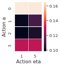
(a) $s_{t}=(3,0)$

(b) $s_{t}=(2,0),\ \eta_{t}=1$

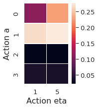
(c) $s_{t}=(2,1),\ \eta_{t}=5$

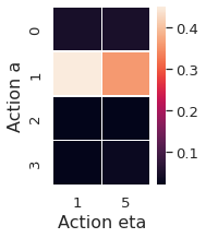
(d) $s_{t}=(2,2),\ \eta_{t}=5$

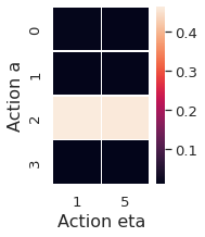
(e) $s_{t}=(2,3),\ \eta_{t}=1$

Figure 7: For $\lambda=0$, the learned optimal path is $[3,0]\to[2,0]\to[2,1]\to[2,2]\to[2,3]\to[3,3]$.

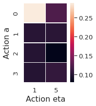
(a) $s_{t}=(3,0)$

(b) $s_{t}=(2,0),\ \eta_{t}=1$

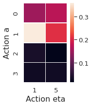
(c) $s_{t}=(2,1),\ \eta_{t}=5$

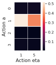
(d) $s_{t}=(2,2),\ \eta_{t}=1$

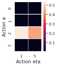
(e) $s_{t}=(2,3),\ \eta_{t}=1$

Figure 8: For $\lambda=0.25$, the learned optimal path is $[3,0]\to[2,0]\to[2,1]\to[2,2]\to[2,3]\to[3,3]$.

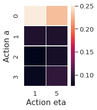
(a) $s_{t}=(3,0)$

(b) $s_{t}=(2,0),\ \eta_{t}=1$

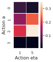
(c) $s_{t}=(1,0),\ \eta_{t}=1$

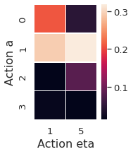
(d) $s_{t}=(2,0),\ \eta_{t}=5$

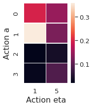
(e) $s_{t}=(2,1),\ \eta_{t}=5$

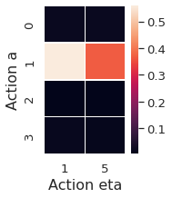
(f) $s_{t}=(2,2),\ \eta_{t}=1$

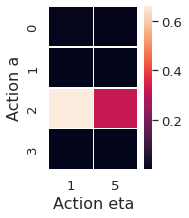
(g) $s_{t}=(2,3),\ \eta_{t}=1$

Figure 9: For $\lambda=0.5$, the learned optimal path is $[3,0]\to[2,0]\to[1,0]\to[2,0]\to[2,1]\to[2,2]\to[2,3]\to[3,3]$.

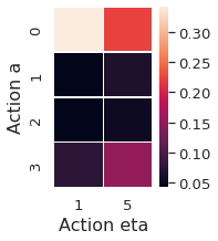
(a) $s_{t}=(3,0)$

(b) $s_{t}=(2,0),\ \eta_{t}=1$

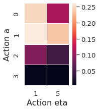
(c) $s_{t}=(1,0),\ \eta_{t}=1$

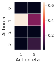
(d) $s_{t}=(1,1),\ \eta_{t}=1$

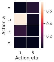
(e) $s_{t}=(1,2),\ \eta_{t}=1$

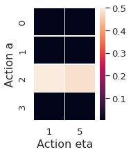
(f) $s_{t}=(1,3),\ \eta_{t}=1$

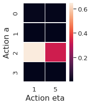
(g) $s_{t}=(2,3),\ \eta_{t}=1$

Figure 10: For $\lambda=0.75$, the learned optimal path is $[3,0]\to[2,0]\to[1,0]\to[1,1]\to[1,2]\to[1,3]\to[2,3]\to[3,3]$.

(a) $s_{t}=(3,0)$

(b) $s_{t}=(2,0),\ \eta_{t}=1$

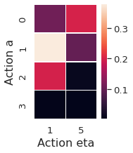
(c) $s_{t}=(1,0),\ \eta_{t}=1$

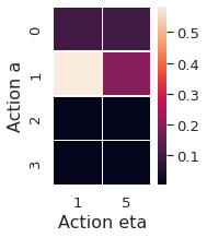
(d) $s_{t}=(1,1),\ \eta_{t}=1$

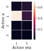
(e) $s_{t}=(1,2),\ \eta_{t}=1$

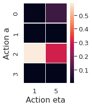
(f) $s_{t}=(1,3),\ \eta_{t}=1$

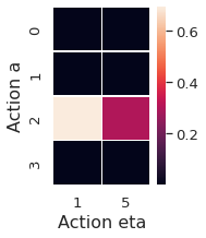
(g) $s_{t}=(2,3),\ \eta_{t}=1$

Figure 11: For $\lambda=1$, the learned optimal path is $[3,0]\to[2,0]\to[1,0]\to[1,1]\to[1,2]\to[1,3]\to[2,3]\to[3,3]$.

References

- Agarwal et al. (2021) Agarwal, A., Kakade, S. M., Lee, J. D., and Mahajan, G. On the theory of policy gradient methods: Optimality, approximation, and distribution shift. Journal of Machine Learning Research, 22(98):1–76, 2021.
- Artzner et al. (1999) Artzner, P., Delbaen, F., Eber, J.-M., and Heath, D. Coherent measures of risk. Mathematical Finance, 9(3):203–228, 1999.
- Barto et al. (1983) Barto, A. G., Sutton, R. S., and Anderson, C. W. Neuronlike adaptive elements that can solve difficult learning control problems. IEEE Transactions on Systems, Man, and Cybernetics, 13(5):834–846, 1983.
- Beck (2017) Beck, A. First-order methods in optimization. SIAM, 2017.
- Bellemare et al. (2017) Bellemare, M. G., Dabney, W., and Munos, R. A distributional perspective on reinforcement learning. In International Conference on Machine Learning, pp. 449–458. PMLR, 2017.
- Bellman & Dreyfus (1959) Bellman, R. and Dreyfus, S. Functional approximations and dynamic programming. Mathematical Tables and Other Aids to Computation, pp. 247–251, 1959.
- Bhandari & Russo (2019) Bhandari, J. and Russo, D. Global optimality guarantees for policy gradient methods. arXiv preprint arXiv:1906.01786, 2019.
- Borkar (2002) Borkar, V. S. Q-learning for risk-sensitive control. Mathematics of Operations Research, 27(2):294–311, 2002.
- Cen et al. (2022) Cen, S., Cheng, C., Chen, Y., Wei, Y., and Chi, Y. Fast global convergence of natural policy gradient methods with entropy regularization. Operations Research, 70(4):2563–2578, 2022.
- Chow & Ghavamzadeh (2014) Chow, Y. and Ghavamzadeh, M. Algorithms for CVaR optimization in MDPs. Advances in Neural Information Processing Systems, 27, 2014.
- Chow & Pavone (2013) Chow, Y.-L. and Pavone, M. Stochastic optimal control with dynamic, time-consistent risk constraints. In 2013 American Control Conference, pp. 390–395. IEEE, 2013.
- Chow & Pavone (2014) Chow, Y.-L. and Pavone, M. A framework for time-consistent, risk-averse model predictive control: Theory and algorithms. In 2014 American Control Conference, pp. 4204–4211. IEEE, 2014.
- Coraluppi & Marcus (2000) Coraluppi, S. P. and Marcus, S. I. Mixed risk-neutral/minimax control of discrete-time, finite-state markov decision processes. IEEE Transactions on Automatic Control, 45(3):528–532, 2000.
- Ghadimi & Lan (2016) Ghadimi, S. and Lan, G. Accelerated gradient methods for nonconvex nonlinear and stochastic programming. Mathematical Programming, 156(1):59–99, 2016.
- Heger (1994) Heger, M. Consideration of risk in reinforcement learning. In Machine Learning Proceedings 1994, pp. 105–111. Elsevier, 1994.
- Homem-de Mello & Pagnoncelli (2016) Homem-de Mello, T. and Pagnoncelli, B. K. Risk aversion in multistage stochastic programming: A modeling and algorithmic perspective. European Journal of Operational Research, 249(1):188–199, 2016.
- Howard & Matheson (1972) Howard, R. A. and Matheson, J. E. Risk-sensitive Markov decision processes. Management Science, 18(7):356–369, 1972.
- Huang et al. (2021) Huang, A., Leqi, L., Lipton, Z. C., and Azizzadenesheli, K. On the convergence and optimality of policy gradient for markov coherent risk. arXiv preprint arXiv:2103.02827, 2021.
- Konda & Tsitsiklis (1999) Konda, V. and Tsitsiklis, J. Actor-critic algorithms. Advances in neural information processing systems, 12, 1999.
- Köse & Ruszczyński (2021) Köse, Ü. and Ruszczyński, A. Risk-averse learning by temporal difference methods with markov risk measures. The Journal of Machine Learning Research, 22(1):1800–1833, 2021.
- La & Ghavamzadeh (2013) La, P. and Ghavamzadeh, M. Actor-critic algorithms for risk-sensitive MDPs. Advances in neural information processing systems, 26, 2013.
- Markowitz & Todd (2000) Markowitz, H. M. and Todd, G. P. Mean-variance analysis in portfolio choice and capital markets, volume 66. John Wiley & Sons, 2000.
- Mei et al. (2020) Mei, J., Xiao, C., Szepesvari, C., and Schuurmans, D. On the global convergence rates of softmax policy gradient methods. In International Conference on Machine Learning, pp. 6820–6829. PMLR, 2020.
- Polyak (1963) Polyak, B. T. Gradient methods for minimizing functionals. USSR Computational Mathematics and Mathematical Physics, 3(4):643–653, 1963.
- Puterman (2014) Puterman, M. L. Markov Decision Processes: Discrete Stochastic Dynamic Programming. John Wiley & Sons, 2014.
- Rockafellar & Uryasev (2002) Rockafellar, R. T. and Uryasev, S. Conditional value-at-risk for general loss distributions. Journal of Banking & Finance, 26(7):1443–1471, 2002.
- Rockafellar et al. (2000) Rockafellar, R. T., Uryasev, S., et al. Optimization of conditional value-at-risk. Journal of Risk, 2(3):21–42, 2000.
- Ruszczyński (2010) Ruszczyński, A. Risk-averse dynamic programming for Markov decision processes. Mathematical Programming, 125(2):235–261, 2010.
- Ruszczyński & Shapiro (2006) Ruszczyński, A. and Shapiro, A. Optimization of convex risk functions. Mathematics of Operations Research, 31(3):433–452, 2006.
- Shapiro et al. (2009) Shapiro, A., Dentcheva, D., and Ruszczyński, A. Lectures on Stochastic Programming: Modeling and Theory. SIAM, 2009.
- Sutton & Barto (2018) Sutton, R. S. and Barto, A. G. Reinforcement Learning: An Introduction. MIT Press, 2018.
- Sutton et al. (1999) Sutton, R. S., McAllester, D., Singh, S., and Mansour, Y. Policy gradient methods for reinforcement learning with function approximation. Advances in Neural Information Processing Systems, 12, 1999.
- Tamar et al. (2012) Tamar, A., Di Castro, D., and Mannor, S. Policy gradients with variance related risk criteria. In Proceedings of the 29th International Coference on International Conference on Machine Learning, pp. 1651–1658, 2012.
- Tamar et al. (2015a) Tamar, A., Chow, Y., Ghavamzadeh, M., and Mannor, S. Policy gradient for coherent risk measures. Advances in Neural Information Processing Systems, 28, 2015a.
- Tamar et al. (2015b) Tamar, A., Glassner, Y., and Mannor, S. Optimizing the CVaR via sampling. In Twenty-Ninth AAAI Conference on Artificial Intelligence, 2015b.
- Williams (1992) Williams, R. J. Simple statistical gradient-following algorithms for connectionist reinforcement learning. Machine Learning, 8(3):229–256, 1992.
- Yu et al. (2017) Yu, P., Haskell, W. B., and Xu, H. Dynamic programming for risk-aware sequential optimization. In 2017 IEEE 56th Annual Conference on Decision and Control (CDC), pp. 4934–4939. IEEE, 2017.
- Yu & Shen (2022) Yu, X. and Shen, S. Risk-averse reinforcement learning via dynamic time-consistent risk measures. In 2022 IEEE 61st Conference on Decision and Control (CDC), pp. 2307–2312, 2022. doi: 10.1109/CDC51059.2022.9992450.