Generalised Geometric Phase

Abstract

A generalised notion of geometric phase for pure states is proposed and its physical manifestations are shown. An appreciation of fact that the interference phenomenon also manifests in the average of an observable, allows us to define the argument of the matrix element of an observable as a generalised relative phase. This identification naturally paves the way for defining an operator generalisation of the geometric phase following Pancharatnam. The notion of natural connection finds an appropriate operator generalisation, and the generalised geometric phase is indeed found to be the (an)holonomy of the generalised connection. It is shown that in scenarios wherein the usual geometric phase is not defined, the generalised geometric phase manifests as a global phase acquired by a quantum state in course of time evolution. The generalised geometric phase is found to contribute to the shift in the energy spectrum due perturbation, and to the forward scattering amplitude in a scattering problem.

I Introduction

It is well known that the notion of geometric phase came to prominence from the celebrated work of Berry Berry (1984). Berry showed that a quantum state acquired a non-trivial global phase, which was of purely geometric origin, when the system was evolved in an adiabatic cyclic manner to return to its initial configuration. The importance of this concept was immediately appreciated by the scientific community, and a flurry of activity followed soon after this landmark work Shapere and Wilczek (1989); Anandan et al. (1997); Anandan (1992). The notion of geometric phase was soon generalised to include scenarios wherein the adiabaticity is absent Aharonov and Anandan (1987). Eventually it was also generalised to scenarios wherein the requirement of cyclicity was also absent Samuel and Bhandari (1988). The mathematical framework behind the occurrence of the geometric phase also got slowly unfolded Simon (1983); Page (1987); Mukunda and Simon (1993). The grounding of the notion of geometric phase got even further cemented by the experimental confirmation of this notion in classical optical systems Chyba et al. (1988); Tomita and Chiao (1986); Chiao et al. (1988) and quantum systems like diatomic molecules and spin half particlesMead (1992); Zwanziger et al. (1990); Bitter and Dubbers (1987). The relevance and importance of geometric phase in classical mechanical systems also received significant attention Agarwal and Simon (1990); Hannay (1985); Chaturvedi et al. (1987); Littlejohn (1988); Anandan (1988); Pati (1998), as also in the context of particle physics Wilczek and Zee (1984); Sonoda (1986); Stone and Goff (1988); Stone (1986). The importance of geometric phase in understanding condensed matter systems was noted immediately after Berry’s work Stone (1986); Wilczek and Zee (1984); Thouless (1983); Simon (1983); Mathur (1991) and forms the pillar of the current understanding of the physics of topological materials and quantum Hall effect, as also that of exotic objects like anyons Thouless et al. (1982); Niu et al. (1985); Bernevig (2013); Shapere and Wilczek (1989); Vyas and Roy (2019, 2021).

As noted by Berry Berry (1990, 1987), the concept of geometric phase had been anticipated independently by several preceding workers starting from Hamilton. One of the elegant ways of understanding the occurrence of the geometric phase in its generality, is due to Pancharatnam, solely based on the phenomenon of interference. This line of thought has turned out to be rewarding and has paved the way for a general setting for the geometric phase, wherein the evolution of the system need not be unitary, adiabatic or cyclic Samuel and Bhandari (1988); Bhandari and Samuel (1988). This development eventually led to a purely kinematic understanding of the geometric phase Mukunda and Simon (1993); Mukunda et al. (2003).

The essence of Pancharatnam’s approach to arrive at the geometric phase lies in the concept of relative phase, defined as $\text{Arg}\langle A\lvert B\rangle$, which provides a scheme of comparison of any two non-orthogonal unit vectors $\lvert A\rangle$ and $\lvert B\rangle$. The usage of relative phase originates from the fact that the interference extrema as observed in the squared norm $\langle A+B\lvert A+B\rangle$ of the superposed vector $\lvert A+B\rangle$ is determined by the relative phase $\text{Arg}\langle A\lvert B\rangle$. For a set of three non-orthogonal unit vectors, Pancharatnam’s definition of the geometric phase is simply the sum of the corresponding relative phases.

It is worth recollecting that apart from the squared norm $\langle A+B\lvert A+B\rangle$, the interference phenomenon also manifests in the average $\langle A+B\lvert\mathscr{O}\lvert A+B\rangle$ of any observable $\mathscr{O}$. The interference extrema in such case is captured by the argument of the matrix element of the observable $\text{Arg}\langle A\lvert\mathscr{O}\lvert B\rangle$. Here we propose that this phase can be understood as an operator generalised relative phase, and can be used as a prescription to compare the vectors $\lvert A\rangle$ and $\lvert B\rangle$. Employing this generalised relative phase, following Pancharatnam’s trail, we are led to the construction of a generalised notion of geometric phase. We find that for a given set of $N$ states, this generalised geometric phase can be constructed for any observable of interest in the system at hand. The generalised geometric phase is found to go over to the usual geometric phase when the observable is taken as identity. We show that the concepts like natural connection and null phase curves, which are used to understand the usual geometric phase, also find an appropriate generalisation. We explicitly show that the generalised geometric phase is the (an)holonomy of the generalised natural connection.

One might wonder if this generalised geometric phase has any physical relevance, or it is just a theoretical construct. Interestingly we find that the generalised geometric phase can manifest in any general quantum system as a global phase acquired in course of time evolution, in scenarios wherein the usual geometric phase is undefined. We also find that within the framework of time independent perturbation theory, the change in the energy levels due to the perturbation has a contribution due to the generalised geometric phase. The survival amplitude for a given state in a quantum system, subjected to a time dependent perturbation, is also found to have a contribution due to the generalised geometric phase. Remarkably in the context of scattering theory, we find that the generalised geometric phase manifests in the total scattering cross section as well as in the forward scattering amplitude.

The notion of geometric phase as understood using the kinematic framework is briefly reviewed in Section (II). In Section (III), the notions of generalised relative phase and generalised geometric phase are introduced and studied. In Section (IV) we discuss the physical manifestations of the generalised geometric phase, and end the article with the summary of the obtained results.

II Review of the notion of Geometric Phase

The concept of geometric phase can be understood elegantly from the viewpoint of Pancharatnam, whose origin lies in the interference phenomenon Pancharatnam (1956); Ramaseshan and Nityananda (1986); Samuel and Bhandari (1988); Bhandari and Samuel (1988). Consider that we have some general physical system given to us, for example classical light beam or quantum point particle, which admits a Hilbert space $\mathscr{H}$. We assume that the system can be prepared in two different states depicted by $\lvert\psi_{1}\rangle$ and $\lvert\psi_{2}\rangle$ respectively. Now if the system is allowed to be in a linearly superposed state $\lvert\psi\rangle=\lvert\psi_{1}\rangle+\lvert\psi_{2}\rangle$, then it is well known that the interference phenomenon manifests in the squared norm of $\lvert\psi\rangle$ (identified with probability in quantum systems and light intensity in optical systems) :

$$\langle\psi\lvert\psi\rangle=\langle\psi_{1}\lvert\psi_{1}\rangle+\langle\psi_{2}\lvert\psi_{2}\rangle+2|\langle\psi_{1}\lvert\psi_{2}\rangle|\cos\left(\text{Arg}\langle\psi_{1}\lvert\psi_{2}\rangle\right).$$ (1)

The phase $\text{Arg}\langle\psi_{1}\lvert\psi_{2}\rangle$ is the relative phase, which gives rise to the periodic extrema in the $\langle\psi\lvert\psi\rangle$. The relative phase captures only the phase difference between the two states, which is evident from the fact that under a global phase transformation $\lvert\psi_{i}\rangle\rightarrow e^{i\lambda_{i}}\lvert\psi_{i}\rangle$ (here $i=1,2$) for some real values of $\lambda_{i}$, the relative phase changes by amount $(\lambda_{2}-\lambda_{1})$. However it must be kept in mind that the interference phenomenon in $\langle\psi\lvert\psi\rangle$ is non-existent if the two states $\lvert\psi_{1}\rangle$ and $\lvert\psi_{2}\rangle$ are orthogonal. The concept of relative phase was used by Pancharatnam to provide a prescription for comparing any two vectors in the Hilbert space. Two vectors are said to be “in-phase” in the sense of Pancharatnam if $\langle\psi_{1}\lvert\psi_{2}\rangle$ is real and positive, that is, if the relative phase $\text{Arg}\langle\psi_{1}\lvert\psi_{2}\rangle$ is zero Pancharatnam (1956); Samuel and Bhandari (1988).

Now suppose we consider three possible states $\lvert\psi_{1}\rangle$, $\lvert\psi_{2}\rangle$ and $\lvert\psi_{3}\rangle$ of the system, all belonging to $\mathscr{H}$. Given that $\lvert\psi_{1}\rangle$ is in-phase with $\lvert\psi_{2}\rangle$, and $\lvert\psi_{2}\rangle$ is in-phase with $\lvert\psi_{3}\rangle$, it is natural to wonder if $\lvert\psi_{1}\rangle$ and $\lvert\psi_{3}\rangle$ are also required to be in-phase. It was found that the in-phase property is non-transitive, and the states $\lvert\psi_{1}\rangle$ and $\lvert\psi_{3}\rangle$ in general need not be in-phase with one another. The three states will be in-phase with one another if the sum of the relative phases $\text{Arg}\langle\psi_{1}\lvert\psi_{2}\rangle+\text{Arg}\langle\psi_{2}\lvert\psi_{3}\rangle+\text{Arg}\langle\psi_{3}\lvert\psi_{1}\rangle$ vanishes. It can be checked that while the individual relative phase can be altered by global phase changes $\lvert\psi_{j}\rangle\rightarrow e^{i\lambda_{j}}\lvert\psi_{j}\rangle$ (where $j=1,2,3$) for some real numbers $\lambda_{j}$, the sum total is unaltered. This sum was used by Pancharatnam Pancharatnam (1956); Samuel and Bhandari (1988); Bhandari and Samuel (1988); Mukunda and Simon (1993), who called it the excess phase, as a measure of deviation of these states from the mutual in-phase configuration. It is generally expressed as:

$$\gamma=\text{Arg}\left(\frac{\langle\psi_{1}\lvert\psi_{2}\rangle\langle\psi_{2}\lvert\psi_{3}\rangle\langle\psi_{3}\lvert\psi_{1}\rangle}{\langle\psi_{1}\lvert\psi_{1}\rangle\langle\psi_{2}\lvert\psi_{2}\rangle\langle\psi_{3}\lvert\psi_{3}\rangle}\right).$$ (2)

The invariance of $\gamma$ under three independent global phase transformations establishes the geometric nature of this phase, and hence it is called the geometric phase Berry (1987); Mukunda and Simon (1993); Samuel and Bhandari (1988). The geometric nature become even more apparent by working with the density matrices $\rho_{j}=\frac{\lvert\psi_{j}\rangle\langle\psi_{j}\rvert}{\langle\psi_{j}\lvert\psi_{j}\rangle}$ corresponding to the states $\lvert\psi_{j}\rangle$, so that (2) now reads:

$$\gamma=\text{Arg}\>\text{Tr}\left(\rho_{1}\rho_{2}\rho_{3}\right).$$ (3)

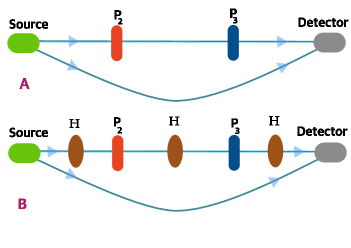
Figure 1: Schematic representation of the experimental setups to observe the geometric phases. Setup $A$ was used to measure the geometric phase $\gamma$ whereas setup $B$ is designed to provide the measurement of generalised geometric phase $\gamma_{H}$. Here $P_{2}$ and $P_{3}$ respectively are devices which project the system onto $\lvert\psi_{2}\rangle$ and $\lvert\psi_{3}\rangle$. The objects $H$ schematically represent the action of the medium on the system, which is akin to the generator of time evolution $H$.

An experimental scheme based on interferometry to observe such a geometric phase was suggested in Ref. Samuel and Bhandari (1988) and it is worth recollecting here. As schematically depicted in setup $A$ in Fig. 1, suppose one prepares a quantum system at hand in state $\lvert\psi_{1}\rangle$ using some source. The setup is so arranged that there is negligible state evolution in the course of the experiment. Subsequently the system is subjected to a measurement using a device $P_{2}$ projecting it along $\lvert\psi_{2}\rangle$ followed by a measurement along $\lvert\psi_{3}\rangle$ using device $P_{3}$. In such a scenario the state of the system is $\lvert\psi_{3}\rangle\langle\psi_{3}\lvert\psi_{2}\rangle\langle\psi_{2}\lvert\psi_{1}\rangle$. Now if the system is allowed to interfere with the initial state $\lvert\psi_{1}\rangle$ then the relative phase measured by the detector turns out to be $\gamma$ which is experimentally measurable. Interestingly such a geometric phase was experimentally observed using an optical interferometer in Ref. Bhandari and Samuel (1988), exploiting the polarisation states of light.

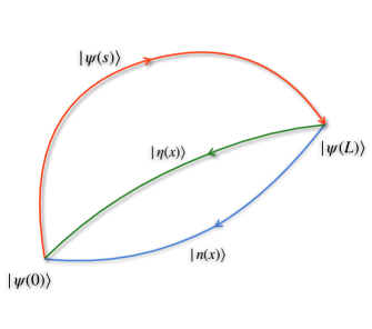
Figure 2: Schematic representation of the integration path in the Hilbert space for evaluating the geometric phase. For evaluating $\gamma(0,L)$ the path is along $\lvert\psi(x)\rangle$ (in red colour) and the null phase curve $\lvert\eta(x)\rangle$ (in green colour). While for evaluating $\gamma_{\mathscr{O}}(0,L)$ the path is along $\lvert\psi(x)\rangle$ and $\mathscr{O}$ null phase curve $\lvert n(x)\rangle$ (in blue colour).

This notion of geometric phase also holds for a collection of $N$ states $\{\lvert\psi_{l}\rangle\}$ which belong to $\mathscr{H}$ (where $l=1,2,\cdots,N$), and it reads:

$$\gamma_{N}=\text{Arg}\left(\frac{\langle\psi_{1}\lvert\psi_{2}\rangle\langle\psi_{2}\lvert\psi_{3}\rangle\cdots\langle\psi_{N-1}\lvert\psi_{N}\rangle\langle\psi_{N}\lvert\psi_{1}\rangle}{\langle\psi_{1}\lvert\psi_{1}\rangle\langle\psi_{2}\lvert\psi_{2}\rangle\langle\psi_{3}\lvert\psi_{3}\rangle\cdots\langle\psi_{N}\lvert\psi_{N}\rangle}\right).$$ (4)

Evidently this notion of geometric phase can not be defined if any of the inner products in the numerator vanish.

A special case of the above expression is when these $N$ states arise from the change of a continuous parameter $s$ ($0\leq s\leq L$) such that $\lvert\psi_{l}\rangle\equiv\lvert\psi(s_{l})\rangle$, where $s_{l}=\frac{(l-1)}{(N-1)}\times L$. In large $N$ limit, the expression for the geometric phase reads:

$$\gamma(0,L)=\text{Arg}\left(\frac{\langle\psi(L)\lvert\psi(0)\rangle}{\langle\psi(L)\lvert\psi(L)\rangle}\right)+\int_{0}^{L}\>ds\>\text{Im}\left(\frac{\langle\psi(s)\lvert d_{s}\psi(s)\rangle}{\langle\psi(s)\lvert\psi(s)\rangle}\right),$$ (5)

where $\lvert d_{s}\psi(s)\rangle\equiv\frac{d}{ds}\lvert\psi(s)\rangle$. The object $A_{\psi}(s)=\text{Im}\left(\frac{\langle\psi(s)\lvert d_{s}\psi(s)\rangle}{\langle\psi(s)\lvert\psi(s)\rangle}\right)$ is often referred to as Berry potential Shapere and Wilczek (1989) and also as natural connection in the literature Simon (1983); Mukunda and Simon (1993); Samuel and Bhandari (1988).

It can be readily checked that this geometric phase is invariant under local gauge transformation: $\lvert\psi(s)\rangle\rightarrow e^{i\lambda(s)}\lvert\psi(s)\rangle$, for any function $\lambda(s)$, since the connection transforms as $A_{\psi}(s)\rightarrow A_{\psi}(s)+d_{s}\lambda(s)$. It can also be readily checked that the geometric phase is invariant under the reparametrization $s\rightarrow r(s)$ (here $r(s)$ is a monotonically increasing function) such that $\lvert\psi(s)\rangle=\lvert\phi(r)\rangle$. These two invariances are a testimony to the geometric nature of this phase Samuel and Bhandari (1988); Mukunda and Simon (1993). It must be noted that this notion of geometric phase is not defined if the initial and final states are orthogonal, as also if any two states $\lvert\psi(s_{l})\rangle$ and $\lvert\psi(s_{l+1})\rangle$ are orthogonal. This is because our notion of relative phase fails for two linearly superposed orthogonal states.

A very important and interesting scenario happens when the states $\lvert\psi(s)\rangle$ occur as an instantaneous eigenstate of the Hamiltonian $H(s)$, that is $H(s)\lvert\psi(s)\rangle=E(s)\lvert\psi(s)\rangle$, where $s$ is some slowly varying parameter in the system. Further if the Hamiltonian is cyclic in $s$ so that $H(0)=H(L)$, then one wonders what happens to the system when it is initially prepared in $\lvert\psi(0)\rangle$, and $s$ is changed from $0$ to $L$ adiabatically. In a celebrated work Berry Berry (1984, 1987) showed that the system will indeed return to $\lvert\psi(0)\rangle$ after a circuit, albeit with an overall phase which has a geometric component give by $\gamma(0,L)$ as expressed in (5). It is evident that if the state $\lvert\psi(s)\rangle$ changes in such a manner that all through out it is parallel to itself, which is ensured if $\text{Im}\langle\psi(s)\lvert d_{s}\psi(s)\rangle=0$, then the relative phase $\text{Arg}\langle\psi(L)\lvert\psi(0)\rangle$ is the geometric phase $\gamma(0,L)$ Simon (1983); Anandan (1992).

It must be noted that the expression (5) is a general expression for the geometric phase acquired by the state of the system, and it is applicable to scenarios wherein the state evolution is neither cyclic, adiabatic or unitary Aharonov and Anandan (1987); Samuel and Bhandari (1988); Mukunda and Simon (1993).

Suppose one is given a set of states $\lvert\eta(x)\rangle$ where $0\leq x\leq\tau$, which defines a continuous curve in the Hilbert space, such that the geometric phase $\gamma(0,\tau)=0$. We have in such a case:

$$\text{Arg}\left(\frac{\langle\eta(0)\lvert\eta(\tau)\rangle}{\langle\eta(\tau)\lvert\eta(\tau)\rangle}\right)=\int_{0}^{\tau}dx\>\text{Im}\left(\frac{\langle\eta(x)\lvert d_{x}\eta(x)\rangle}{\langle\eta(x)\lvert\eta(x)\rangle}\right).$$ (6)

Such curves are of special relevance in the understanding of geometric phase, and are called null phase curves Mukunda et al. (2003); Chaturvedi et al. (2013); Mittal et al. (2022). The above expression tell us that the relative phase $\text{Arg}\langle\eta(0)\lvert\eta(\tau)\rangle$ is expressible as a line integral of the natural connection over the null phase curve. A classic result of Ref. Samuel and Bhandari (1988) shows the existence and construction of such a curve connecting any two non-orthogonal states $\lvert A\rangle$ and $\lvert B\rangle$ in the Hilbert space . It was shown that there exists a curve $\lvert\bar{\eta}(x)\rangle$ where:

$$\lvert\bar{\eta}(x)\rangle=\frac{e^{i\theta x/\tau}}{\sin\tau}\left(\sin(\tau-x)\lvert A\rangle+e^{-i\theta}\sin(x)\lvert B\rangle\right),$$ (7)

such that the relative phase between the two states $\theta=\text{Arg}\langle B\lvert A\rangle$ can be expressed as an integral of natural connection $\text{Im}\left(\frac{\langle\bar{\eta}(x)\lvert d_{x}\bar{\eta}(x)\rangle}{\langle\bar{\eta}(x)\lvert\bar{\eta}(x)\rangle}\right)$ along the curve $\lvert\bar{\eta}(x)\rangle$ connecting them Samuel and Bhandari (1988); Mukunda and Simon (1993); Mukunda et al. (2003).

The special importance of these null phase curves also stems from the fact that if one is provided with a continuous curve $\lvert\psi(s)\rangle$ ($0\leq s\leq L$) for which the geometric phase is $\gamma(0,L)$, and a null phase curve $\lvert\eta(x)\rangle$ (where $0\leq x\leq\tau$) such that $\lvert\eta(0)\rangle=\lvert\psi(L)\rangle$ and $\lvert\eta(\tau)\rangle=\lvert\psi(0)\rangle$, then $\gamma(0,L)$ can be expressed as a closed loop integral of the natural connection:

$$\gamma(0,L) =\int_{0}^{L}ds\>A_{\psi}(s)+\int_{0}^{\tau}dx\>A_{\eta}(x)$$

$$\equiv\oint_{C}dl\>A(l).$$ (8)

Here the integrands are given by $A_{\psi}(s)=\text{Im}\left(\frac{\langle\psi(s)\lvert d_{s}\psi(s)\rangle}{\langle\psi(s)\lvert\psi(s)\rangle}\right)$ and $A_{\eta}(x)=\text{Im}\left(\frac{\langle\eta(x)\lvert d_{x}\eta(x)\rangle}{\langle\eta(x)\lvert\eta(x)\rangle}\right)$. The curve $C$ is specified from $\lvert\psi(0)\rangle$ to $\lvert\psi(L)\rangle$ through $\lvert\psi(s)\rangle$, whereas from $\lvert\psi(L)\rangle$ to $\lvert\psi(0)\rangle$ through $\lvert\eta(x)\rangle$, as depicted in Fig. 2. This expression indicates that the geometric phase is actually the (an)holonomy of the natural connection Berry (1990); Anandan (1992).

III Generalised Geometric Phase

Generalisation of relative phase

In the earlier section, we began our discussion on the concept of interference by investigating the behaviour of $\langle\psi\lvert\psi\rangle$ as a function of relative phase $\text{Arg}\langle\psi_{1}\lvert\psi_{2}\rangle$ (as seen in (1)). It is on this edifice that most of the interference phenomena are understood in quantum physics as also in optics Sakurai and Commins (1995); Agarwal (2012); Born and Wolf (2013); Feynman et al. (1998); Esposito et al. (2004). A careful reflection reveals that the phenomena of interference has manifestations beyond the probability or intensity. Apart from squared norm $\langle\phi\lvert\phi\rangle$, nature permits us to measure the average $\langle\mathscr{O}\rangle_{\phi}=\frac{\langle\phi\lvert\mathscr{O}\lvert\phi\rangle}{\langle\phi\lvert\phi\rangle}$ corresponding to an observable $\mathscr{O}$ when the system at hand is in the state $\lvert\phi\rangle$ . The average of observable $\mathscr{O}$ in a unit normalised superposed state $\lvert\psi\rangle=\lvert\psi_{1}\rangle+\lvert\psi_{2}\rangle$, is given by:

$$\langle\mathscr{O}\rangle_{\psi} ={\langle\psi\lvert\mathscr{O}\lvert\psi\rangle}$$

$$=\langle\psi_{1}\lvert\mathscr{O}\lvert\psi_{1}\rangle+\langle\psi_{2}\lvert\mathscr{O}\lvert\psi_{2}\rangle+2|\langle\psi_{1}\lvert\mathscr{O}\lvert\psi_{2}\rangle|\cos\left(\text{Arg}\langle\psi_{1}\lvert\mathscr{O}\lvert\psi_{2}\rangle\right).$$ (9)

Evidently the average of $\mathscr{O}$ experiences periodic extrema as a function of phase $\text{Arg}\langle\psi_{1}\lvert\mathscr{O}\lvert\psi_{2}\rangle$. The phase $\text{Arg}\langle\psi_{1}\lvert\mathscr{O}\lvert\psi_{2}\rangle$ is sensitive to the relative phase change between the states $\lvert\psi_{1}\rangle$ and $\lvert\psi_{2}\rangle$, which can be seen from the fact that under a transformation $\lvert\psi_{2}\rangle\rightarrow e^{i\theta}\lvert\psi_{2}\rangle$ it changes by amount $\theta$. As a result, the phase $\text{Arg}\langle\psi_{1}\lvert\mathscr{O}\lvert\psi_{2}\rangle$ can be thought of as a generalisation of relative phase $\text{Arg}\langle\psi_{1}\lvert\psi_{2}\rangle$. While the relative phase $\text{Arg}\langle\psi_{1}\lvert\psi_{2}\rangle$ governs the interference extrema in $\langle\psi\lvert\psi\rangle$, it is the relative phase $\text{Arg}\langle\psi_{1}\lvert\mathscr{O}\lvert\psi_{2}\rangle$ that determines the extrema in the average $\langle\mathscr{O}\rangle_{\psi}$. It is clear that there is no definite relation between the two relative phases, since the amplitudes $\langle\psi_{1}\lvert\psi_{2}\rangle$ and $\langle\psi_{1}\lvert\mathscr{O}\lvert\psi_{2}\rangle$ are independent of one another.

One can now use this $\mathscr{O}$ relative phase $\text{Arg}\langle\psi_{1}\lvert\mathscr{O}\lvert\psi_{2}\rangle$ as a criteria to define “$\mathscr{O}$ in-phase” condition: the two states $\lvert\psi_{1,2}\rangle$ are said to be “$\mathscr{O}$ in-phase” with one another if $\text{Arg}\langle\psi_{1}\lvert\mathscr{O}\lvert\psi_{2}\rangle$ is zero. It is evident that the two states can be $\mathscr{O}$ in-phase but they need not be $\mathscr{O}^{\prime}$ in-phase for some non-trivial operator $\mathscr{O}\neq\mathscr{O}^{\prime}$, as also the two states need not be in-phase in the Pancharatnam sense with $\langle\psi_{1}\lvert\psi_{2}\rangle$ being real and positive. It must be noted that the relative phase $\text{Arg}\langle\psi_{1}\lvert\psi_{2}\rangle$ is a special case of $\mathscr{O}$ relative phase with $\mathscr{O}=\mathbf{1}$.

Interestingly in the literature the ratio of the two amplitudes $\langle\psi_{1}\lvert\psi_{2}\rangle$ and $\langle\psi_{1}\lvert\mathscr{O}\lvert\psi_{2}\rangle$ has received significant attention and it is called the weak value Dressel et al. (2014); Aharonov et al. (1988); Duck et al. (1989) for observable $\mathscr{O}$:

$$w_{\mathscr{O}}(\psi_{1},\psi_{2})=\frac{\langle\psi_{1}\lvert\mathscr{O}\lvert\psi_{2}\rangle}{\langle\psi_{1}\lvert\psi_{2}\rangle}.$$ (10)

In many experiments such weak values have been experimentally measured Dressel et al. (2014); Ritchie et al. (1991); Hosten and Kwiat (2008); Gorodetski et al. (2012). Evidently the weak value in general is a complex number, and hence its interpretation as an observable quantity within the framework of quantum mechanics has been intensely debated Jozsa (2007); Dressel et al. (2014); Vaidman (2017); Hariri et al. (2019). In light of our conception of $\mathscr{O}$ generalised relative phase $\text{Arg}\langle\psi_{1}\lvert\mathscr{O}\lvert\psi_{2}\rangle$, one immediately sees another physical significance of the argument of the weak value $w_{\mathscr{O}}(\psi_{1},\psi_{2})$, as the difference of the two relative phases:

$$\text{Arg}\>w_{\mathscr{O}}(\psi_{1},\psi_{2})=\text{Arg}\langle\psi_{1}\lvert\mathscr{O}\lvert\psi_{2}\rangle-\text{Arg}\langle\psi_{1}\lvert\psi_{2}\rangle.$$ (11)

If the argument of weak value is zero, then it tells us that the two relative phases are identical, and hence the interference manifestation in squared norm $\langle\phi\lvert\phi\rangle$ and the average $\langle\mathscr{O}\rangle_{\psi}$ is essentially identical. This indicates that the net impact of $\mathscr{O}$ in defining the relative phase $\text{Arg}\langle\psi_{1}\lvert\mathscr{O}\lvert\psi_{2}\rangle$ is akin to identity. On the otherhand, a non-zero value of the argument of weak value implies that the two relative phases are distinct, owing to the non-trivial role played by $\mathscr{O}$. This shows that the argument of weak value actually provides a measure of contribution of $\mathscr{O}$ to the interference phenomenon as observed in $\langle\mathscr{O}\rangle_{\psi}$.

Generalisation of Geometric Phase

With the above generalisation of the notion of relative phase, we are now in the position to generalise the concept of geometric phase, following the foot steps of Pancharatnam. Suppose we are given three possible states $\lvert\psi_{1}\rangle$, $\lvert\psi_{2}\rangle$ and $\lvert\psi_{3}\rangle$ all belonging to $\mathscr{H}$. And we are also provided that $\lvert\psi_{1}\rangle$ is $\mathscr{O}$ in-phase with $\lvert\psi_{2}\rangle$, and $\lvert\psi_{2}\rangle$ is $\mathscr{O}$ in-phase with $\lvert\psi_{3}\rangle$. We now ask whether it implies that $\lvert\psi_{1}\rangle$ and $\lvert\psi_{3}\rangle$ are also $\mathscr{O}$ in-phase. It can be easily checked that the $\mathscr{O}$ in-phase property is non-transitive, and the states $\lvert\psi_{1}\rangle$ and $\lvert\psi_{3}\rangle$ in general need not be $\mathscr{O}$ in-phase with one another. The measure of deviation of these states from mutual $\mathscr{O}$ in-phase configuration will now be captured by:

$$\gamma_{\mathscr{O}} =\text{Arg}\left(\frac{\langle\psi_{1}\lvert\mathscr{O}\lvert\psi_{2}\rangle\langle\psi_{2}\lvert\mathscr{O}\lvert\psi_{3}\rangle\langle\psi_{3}\lvert\mathscr{O}\lvert\psi_{1}\rangle}{\langle\psi_{1}\lvert\psi_{1}\rangle\langle\psi_{2}\lvert\psi_{2}\rangle\langle\psi_{3}\lvert\psi_{3}\rangle}\right)$$ (12)

$$=\text{Arg}\>\text{Tr}\left(\rho_{1}\mathscr{O}\rho_{2}\mathscr{O}\rho_{3}\mathscr{O}\right).$$ (13)

This is the operator generalisation of the concept of geometric phase $\gamma$ as defined in (2). Evidently the operator generalised geometric phase $\gamma_{\mathscr{O}}$ goes over to the usual geometric phase $\gamma$ when $\mathscr{O}=\mathbf{1}$. It can be readily checked that the phase $\gamma_{\mathscr{O}}$ is invariant under the three independent global phase transformations: $\lvert\psi_{j}\rangle\rightarrow e^{i\lambda_{j}}\lvert\psi_{j}\rangle$ (where $j=1,2,3$) for some real numbers $\lambda_{j}$, which is a proof of the geometric nature of $\gamma_{\mathscr{O}}$.

It must be mentioned that the phase $\gamma_{\mathscr{O}}$ is well defined and in general has a distinct value for each given observable $\mathscr{O}$. Employing weak values one finds a relation between the geometric phase $\gamma(\equiv\gamma_{\mathbf{1}})$ and generalised geometric phase $\gamma_{\mathscr{O}}$ as:

$$\gamma_{\mathscr{O}}=\text{Arg}\left(w_{\mathscr{O}}(\psi_{1},\psi_{2})w_{\mathscr{O}}(\psi_{2},\psi_{3})w_{\mathscr{O}}(\psi_{3},\psi_{1})\right)+\gamma,$$ (14)

provided the states $\lvert\psi_{j}\rangle$ are mutually non-orthogonal. In case when any of the states $\lvert\psi_{j}\rangle$ are mutually orthogonal, this identity does not hold.

This notion of geometric phase can also be extended to a collection of $N$ states $\{\lvert\psi_{l}\rangle\}$ which belong to $\mathscr{H}$ (where $l=1,2,\cdots,N$), as follows:

$$\gamma_{\mathscr{O},N}=\text{Arg}\left(\frac{\langle\psi_{1}\lvert\mathscr{O}\lvert\psi_{2}\rangle\langle\psi_{2}\lvert\mathscr{O}\lvert\psi_{3}\rangle\cdots\langle\psi_{N-1}\lvert\mathscr{O}\lvert\psi_{N}\rangle\langle\psi_{N}\lvert\mathscr{O}\lvert\psi_{1}\rangle}{\langle\psi_{1}\lvert\psi_{1}\rangle\langle\psi_{2}\lvert\psi_{2}\rangle\cdots\langle\psi_{N}\lvert\psi_{N}\rangle}\right).$$ (15)

It must be mentioned that this notion of geometric phase can not be defined if any of the amplitudes in the numerator vanish.

Let us consider a special case wherein these $N$ states arise from the change of a continuous parameter $s$ ($0\leq s\leq L$) such that $\lvert\psi_{l}\rangle\equiv\lvert\psi(s_{l})\rangle$, where $s_{l}=\frac{(l-1)}{(N-1)}\times L$. Without loss of generality let us consider $N$ to be odd and large, so that we have:

$$\frac{\langle\psi_{1}\lvert\mathscr{O}\lvert\psi_{2}\rangle\langle\psi_{2}\lvert\mathscr{O}\lvert\psi_{3}\rangle\cdots\langle\psi_{N-1}\lvert\mathscr{O}\lvert\psi_{N}\rangle\langle\psi_{N}\lvert\mathscr{O}\lvert\psi_{1}\rangle}{\langle\psi_{1}\lvert\psi_{1}\rangle\langle\psi_{2}\lvert\psi_{2}\rangle\cdots\langle\psi_{N}\lvert\psi_{N}\rangle}$$

$$=\left(\prod_{l=1}^{N-1}\frac{\langle\psi_{l}\lvert\mathscr{O}\lvert\psi_{l}\rangle}{\langle\psi_{l}\lvert\psi_{l}\rangle}\right)\left(\frac{\langle\psi_{N}\lvert\mathscr{O}\lvert\psi_{1}\rangle}{\langle\psi_{N}\lvert\psi_{N}\rangle}\>\exp\left\{\int_{0}^{L}\>ds\>\frac{\langle\psi(s)\lvert\mathscr{O}\lvert d_{s}\psi(s)\rangle}{\langle\psi(s)\lvert\mathscr{O}\lvert\psi(s)\rangle}\right\}\right).$$ (16)

Here we have assumed that none of the averages $\langle\psi_{l}\lvert\mathscr{O}\lvert\psi_{l}\rangle$ are vanishing. In light of this expression, the generalised geometric phase $\gamma_{\mathscr{O},N}$ can now be written as:

$$\gamma_{\mathscr{O}}(0,L)=\text{Arg}\left(\frac{\langle\psi(L)\lvert\mathscr{O}\lvert\psi(0)\rangle}{\langle\psi(L)\lvert\psi(L)\rangle}\right)+\int_{0}^{L}\>ds\>\text{Im}\left(\frac{\langle\psi(s)\lvert\mathscr{O}\lvert d_{s}\psi(s)\rangle}{\langle\psi(s)\lvert\mathscr{O}\lvert\psi(s)\rangle}\right).$$ (17)

Here the object $A^{\mathscr{O}}_{\psi}(s)=\text{Im}\left(\frac{\langle\psi(s)\lvert\mathscr{O}\lvert d_{s}\psi(s)\rangle}{\langle\psi(s)\lvert\mathscr{O}\lvert\psi(s)\rangle}\right)$ is the operator generalisation of the natural connection or the Berry potential $A^{\mathbf{1}}_{\psi}(s)\equiv A_{\psi}(s)$ as defined earlier. It can be readily checked that $\gamma_{\mathscr{O}}(0,L)$ is invariant under the local gauge transformation: $\lvert\psi(s)\rangle\rightarrow e^{i\lambda(s)}\lvert\psi(s)\rangle$, for any smooth function $\lambda(s)$, owing to the fact that the generalised connection transforms as $A^{\mathscr{O}}_{\psi}(s)\rightarrow A^{\mathscr{O}}_{\psi}(s)+d_{s}\lambda(s)$. One can also see that the generalised geometric phase is also invariant under the reparametrization $s\rightarrow r(s)$ (where $r(s)$ is a monotonically increasing function) such that $\lvert\psi(s)\rangle=\lvert\phi(r)\rangle$. It is also evident that $\gamma_{\mathscr{O}}(0,L)$ goes over to $\gamma(0,L)$ when $\mathscr{O}=\mathbf{1}$.

The notion of null phase curve can also be extended naturally to the generalised geometric phase $\gamma_{\mathscr{O}}$. For a given continuous curve $\lvert n(x)\rangle$ (where $0\leq x\leq\tau$) if the geometric phase

$$\gamma_{\mathscr{O}}(0,\tau)=\text{Arg}\left(\frac{\langle n(\tau)\lvert\mathscr{O}\lvert n(0)\rangle}{\langle n(\tau)\lvert n(\tau)\rangle}\right)+\int_{0}^{\tau}\>dx\>\text{Im}\left(\frac{\langle n(x)\lvert\mathscr{O}\lvert d_{x}n(x)\rangle}{\langle n(x)\lvert\mathscr{O}\lvert n(x)\rangle}\right),$$ (18)

is zero, then we say that it is $\mathscr{O}$ null phase curve. Since the value of the geometric phase $\gamma(0,\tau)$ (as given by (6)) would in general be different from $\gamma_{\mathscr{O}}(0,\tau)$, a null phase curve corresponding to $\gamma(0,\tau)$ need not be a $\mathscr{O}$ null phase curve, and vice versa.

From the above definition of the null phase curve, it follows that given any two states $\lvert A\rangle$ and $\lvert B\rangle$ in $\mathscr{H}$, there always exists an $\mathscr{O}$ null phase curve that connects them, so long as the amplitude $\langle A\lvert\mathscr{O}\lvert B\rangle\neq 0$. Without loss of generality, let us assume that there exists a curve $\lvert n(x)\rangle$ (where $0\leq x\leq\tau$), such that $\lvert A\rangle\equiv\lvert n(0)\rangle$ and $\lvert B\rangle\equiv\lvert n(\tau)\rangle$. Let us perform a gauge transformation to define a new curve $\lvert N(x)\rangle=e^{i\theta\frac{x}{\tau}}\lvert n(x)\rangle$, where $\theta=\text{Arg}\left(\frac{\langle B\lvert\mathscr{O}\lvert A\rangle}{\langle B\lvert B\rangle}\right)$. One sees that $\text{Arg}\left(\frac{\langle N(\tau)\lvert\mathscr{O}\lvert N(0)\rangle}{\langle N(\tau)\lvert N(\tau)\rangle}\right)=0$, implying that $\langle N(\tau)\lvert\mathscr{O}\lvert N(0)\rangle$ is real and positive. Now let us define the curve as $\lvert N(x)\rangle=(1-\frac{x}{\tau})\lvert N(0)\rangle+\frac{x}{\tau}\lvert N(\tau)\rangle$. One can straight away see that $\text{Im}\left(\frac{\langle N(x)\lvert\mathscr{O}\lvert d_{x}N(x)\rangle}{\langle N(x)\lvert\mathscr{O}\lvert N(x)\rangle}\right)=0$ for this curve. This shows that $\lvert N(x)\rangle$ is a $\mathscr{O}$ null phase curve albeit connecting $\lvert N(0)\rangle=\lvert A\rangle$ to $\lvert N(\tau)\rangle=e^{i\theta}\lvert B\rangle$. Undoing the gauge transformation one obtains the expression for the curve as:

$$\lvert n(x)\rangle=e^{-i\theta\frac{x}{\tau}}\left((1-\frac{x}{\tau})\lvert A\rangle+\frac{x}{\tau}e^{i\theta}\lvert B\rangle\right).$$ (19)

Since the property of having zero geometric phase is invariant under local gauge transformation, one infers that the curve $\lvert n(x)\rangle$ is also a $\mathscr{O}$ null phase curve, which connects $\lvert A\rangle$ to $\lvert B\rangle$. As a result we have that:

$$\text{Arg}\left(\frac{\langle A\lvert\mathscr{O}\lvert B\rangle}{\langle B\lvert B\rangle}\right)=\int_{0}^{\tau}\>dx\>\text{Im}\left(\frac{\langle n(x)\lvert\mathscr{O}\lvert d_{x}n(x)\rangle}{\langle n(x)\lvert\mathscr{O}\lvert n(x)\rangle}\right)$$ (20)

The existence of the $\mathscr{O}$ null phase curve provides one with a pleasing way to express $\gamma_{\mathscr{O}}(0,L)$ as a closed loop integral of the generalised natural connection. Consider that one is given a non-trivial curve $\lvert\psi(s)\rangle$ ($0\leq s\leq L$) as depicted in Fig. 2 connecting $\lvert\psi(0)\rangle$ to $\lvert\psi(L)\rangle$, for the geometric phase is $\gamma_{\mathscr{O}}(0,L)$. Invoking the above construction we obtain a $\mathscr{O}$ null phase curve $\lvert n(x)\rangle$ connecting $\lvert\psi(L)\rangle\equiv\lvert n(0)\rangle$ to $\lvert\psi(0)\rangle\equiv\lvert n(\tau)\rangle$, so that the geometric phase is expressible as:

$$\gamma_{\mathscr{O}}(0,L)= \int_{0}^{L}\>ds\>{A}^{\mathscr{O}}_{\psi}(s)+\int_{0}^{\tau}\>dx\>{A}^{\mathscr{O}}_{n}(x)$$

$$\equiv\oint_{\mathscr{C}}\>dl\>{A}^{\mathscr{O}}(l).$$ (21)

Here we have defined the generalised connection as ${A}^{\mathscr{O}}_{\psi}(s)=\text{Im}\left(\frac{\langle\psi(s)\lvert\mathscr{O}\lvert d_{s}\psi(s)\rangle}{\langle\psi(s)\lvert\mathscr{O}\lvert\psi(s)\rangle}\right)$, and ${A}^{\mathscr{O}}_{n}(x)=\text{Im}\left(\frac{\langle n(x)\lvert\mathscr{O}\lvert d_{x}n(x)\rangle}{\langle n(x)\lvert\mathscr{O}\lvert n(x)\rangle}\right)$. The closed curve $\mathscr{C}$ consists of $\lvert\psi(s)\rangle$ and $\lvert n(x)\rangle$ as depicted in Fig. 2.

Interestingly the existence of a $\mathscr{O}$ null phase between any two states allows us to re-express the generalised geometric phase ${\gamma_{\mathscr{O}}}$ (as defined in (12)) as a closed loop integral along $\Delta$ formed by the three $\mathscr{O}$ null phase curves $\lvert n_{12}(x)\rangle$, $\lvert n_{23}(y)\rangle$ and $\lvert n_{31}(z)\rangle$ (see Fig. 3):

$$\gamma_{\mathscr{O}} =\int_{n_{12}}\>dx\>{A}^{\mathscr{O}}_{12}(x)+\int_{n_{23}}\>dy\>{A}^{\mathscr{O}}_{23}(y)+\int_{n_{31}}\>dz\>{A}^{\mathscr{O}}_{31}(z)$$ (22)

$$\equiv\oint_{\Delta}\>dl\>{A}^{\mathscr{O}}(l).$$ (23)

Here the $\mathscr{O}$ null phase curve $\lvert n_{ij}\rangle$ connects $\lvert\psi_{i}\rangle$ to $\lvert\psi_{j}\rangle$, whereas ${A}^{\mathscr{O}}_{ij}=\text{Im}\left(\frac{\langle n_{ij}(x)\lvert\mathscr{O}\lvert d_{x}n_{ij}(x)\rangle}{\langle n_{ij}(x)\lvert\mathscr{O}\lvert n_{ij}(x)\rangle}\right)$.

This clearly shows that the geometric phase $\gamma_{\mathscr{O}}$ is the (an)holonomy of the generalised connection $A^{\mathscr{O}}$.

IV Physical Manifestions of Generalised Geometric Phase

The reader might wonder whether the geometric phase $\gamma_{\mathscr{O}}$ is just another mathematical construct or if it provides some physical insight about the system at hand. After a careful study we find that the operator generalised geometric phase provides an alternative means of defining the coherence property of the set of states.

Remarkably we find that the generalised geometric phase can arise in any general quantum system in course of time evolution. Assume that we are provided with a system defined by the time independent Hamiltonian $H=H_{0}+H_{\text{int}}$, where $H_{0}$ represents the free part of the Hamiltonian, whereas $H_{\text{int}}$ stands for non-trivial interacting part of $H$. Let three unit normalised orthogonal eigenstates of $H_{0}$ be given by $\lvert 0\rangle$, $\lvert 1\rangle$ and $\lvert 2\rangle$.

Initially let the system be prepared in state $\lvert 0\rangle$ and allowed to evolve for some small time $\varepsilon$. Subsequently let a projective measurement be performed on the system to find that it is in the state $\lvert 1\rangle$ (modulo an overall phase). The system is again allowed to evolve for time $\varepsilon$ before getting subjected to a projective measurement which discovers that it is now in the state $\lvert 2\rangle$ (modulo an overall phase). Now after evolution for time $\varepsilon$ if yet another measurement is performed so as to project it back to $\lvert 0\rangle$, then one finds that the state of the system is given by $\lvert 0\rangle\langle 0\lvert U(3\varepsilon,2\varepsilon)\lvert 2\rangle\langle 2\lvert U(2\varepsilon,\varepsilon)\lvert 1\rangle\langle 1\lvert U(\varepsilon,0)\lvert 0\rangle$. Here we are working in the Schrodinger picture of time evolution, wherein the evolution operator is $U(t_{2},t_{1})=\exp(-\frac{i}{\hbar}(t_{2}-t_{1})H)$. This shows that the system returns to its initial state albeit, to the leading order in $\varepsilon$, acquiring a non-trivial operator generalised geometric phase $\gamma_{H}=\text{Arg}\left(\langle 0\lvert H\lvert 1\rangle\langle 1\lvert H\lvert 2\rangle\langle 2\lvert H\lvert 0\rangle\right)$, where the role of $\mathscr{O}$ is played by $H$. This generalised geometric phase can also be experimentally measured by interferometry wherein the system after time $3\varepsilon$, which is in the state $U(3\varepsilon,2\varepsilon)\lvert 2\rangle\langle 2\lvert U(2\varepsilon,\varepsilon)\lvert 1\rangle\langle 1\lvert U(\varepsilon,0)\lvert 0\rangle$, is allowed to be superposed to $\lvert 0\rangle$. This can be achieved by altering the interferometric setup $A$ depicted in Fig. 1 to setup $B$ by ensuring that the states $\psi_{i}$ are chosen to be orthogonal (and are not eigenstates of $H$), and by introducing a suitable medium which acts on the states as the Hamiltonian operator $H$. As a result the relative phase measured by the detector would be $\gamma_{H}$. It must be mentioned that the usual geometric phase (as given by (12)) is not defined in this scenario since we are dealing with orthogonal states.

This clearly shows that operator generalised geometric phases $\gamma_{\mathscr{O}}$ are not mere theoretical constructs, but are as physical as the (identity) geometric phase $\gamma$.

From the above discussion it is clear that the while there are many possible geometric phases $\gamma_{\mathscr{O}}$ for each choice of $\mathscr{O}$, the physics of the given system determines so as to which geometric phase will be acquired by the state. While in the scenario considered above it is the $\gamma_{H}$ that manifests, in the scenarios considered by Berry and others, it is $\gamma_{\mathbf{1}}$ that is observed.

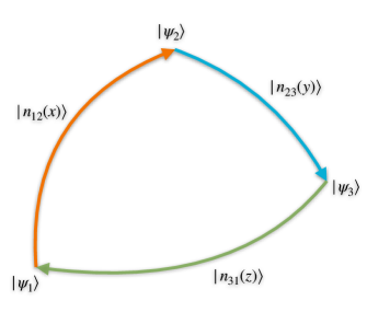
Figure 3: Schematic representation of the integration path in the Hilbert space for evaluating $\gamma_{\mathscr{O}}$ as expressed in (12).

Let us consider the example of a quantum two level system to provide an explicit evaluation of $\gamma_{\mathscr{O}}$. Here we consider the states $\lvert 0\rangle$ and $\lvert 1\rangle$ as the Hamiltonian eigenstates. Suppose one wants to find the geometric phase between the (unit normalised) states $\lvert 0\rangle$, $\lvert\Psi(\theta,\phi)\rangle=\cos\frac{\theta}{2}\lvert 0\rangle+e^{i\phi}\sin\frac{\theta}{2}\lvert 1\rangle$, and $\lvert 1\rangle$. Note that the usual geometric phase $\gamma$ is not defined in this case, since $\langle 0\lvert 1\rangle=0$. However one can use an important observable in the system operator $X=\lvert 1\rangle\langle 0\rvert+\lvert 0\rangle\langle 1\rvert$, which swaps the two eigenstates, to find the corresponding geometric phase. The geometric phase $\gamma_{X}$ is given by:

$$\gamma_{X}=\text{Arg}\left(\langle 0\lvert X\lvert\Psi\rangle\langle\Psi\lvert X\lvert 1\rangle\langle 1\lvert X\lvert 0\rangle\right),$$ (24)

which simplifies to yield: $\gamma_{X}=\phi$ if $0\leq\theta\leq\pi$, and $\gamma_{X}=\pi+\phi$ if $\pi\leq\theta\leq 2\pi$.

In case if one employs the Hadamard operator $H$ which superposes the two eigenstates: $H\lvert 0\rangle=\lvert+\rangle$ and $H\lvert 1\rangle=\lvert-\rangle$, where $\lvert\pm\rangle=\frac{1}{\sqrt{2}}(\lvert 0\rangle\pm\lvert 1\rangle)$, the corresponding geometric phase is defined as:

$$\gamma_{H}=\text{Arg}\left(\langle 0\lvert H\lvert\Psi\rangle\langle\Psi\lvert H\lvert 1\rangle\langle 1\lvert H\lvert 0\rangle\right),$$ (25)

and simplifies to read: $\gamma_{H}=\arctan(\tan\theta\>\sin\phi)$.

The generalised geometric phase also manifests in the survival amplitude for any given quantum state, when studied employing the time dependent perturbation theory Sakurai and Commins (1995). To illustrate this explicitly let us consider a quantum system depicted by time independent Hamiltonian $H_{0}$, with eigenstates $\lvert n^{0}\rangle$: $H_{0}\lvert n^{0}\rangle=E_{n}^{0}\lvert n^{0}\rangle$. Let it be subjected to a time dependent perturbation $H_{\text{int}}(t)$. In the interaction picture it evolves as $H^{I}_{\text{int}}(t)=e^{i\frac{t}{\hbar}H_{0}}H_{\text{int}}(t)e^{-i\frac{t}{\hbar}H_{0}}$. The time evolution operator is given by $U_{I}(t,t_{0})=1-\frac{i}{\hbar}\int_{t_{0}}^{t}ds\>H^{I}_{\text{int}}(s)U_{I}(s,t_{0})$, which evolves any given state from time $t_{0}$ to $t$. Iterating this expression provides us with the Dyson series for $U_{I}(t,t_{0})$ Sakurai and Commins (1995); Gottfried and Yan (2013):

$$U_{I}(t,t_{0})= \>1-\frac{i}{\hbar}\int_{t_{0}}^{t}ds\>H^{I}_{\text{int}}(s)+\left(-\frac{i}{\hbar}\right)^{2}\int_{t_{0}}^{t}ds_{1}\int_{t_{0}}^{s_{1}}ds_{2}\>H^{I}_{\text{int}}(s_{1})H^{I}_{\text{int}}(s_{2})$$

$$+\left(-\frac{i}{\hbar}\right)^{3}\int_{t_{0}}^{t}ds_{1}\int_{t_{0}}^{s_{1}}ds_{2}\int_{t_{0}}^{s_{2}}ds_{3}\>H^{I}_{\text{int}}(s_{1})H^{I}_{\text{int}}(s_{2})H^{I}_{\text{int}}(s_{3})+\cdots.$$ (26)

For simplicity let us consider that a time independent perturbation is switch on at time $t=0$: $H_{\text{int}}(t)=\theta(t)V$. Assuming that the system is prepared to be in state $\lvert i^{0}\rangle$ at time $t_{0}$, the transition amplitude for finding the system in the same state $\lvert i^{0}\rangle$ after time $t$ is given by $\langle i^{0}\lvert U_{I}(t,t_{0})\lvert i^{0}\rangle$, which is called the survival amplitude for $\lvert i^{0}\rangle$. Employing the above expression, we immediately see that the third order contribution to the survival amplitude is given by:

$$\langle i^{0}\lvert U^{(3)}(t,t_{0})\lvert i^{0}\rangle= \>\left(-\frac{i}{\hbar}\right)^{3}\int_{t_{0}}^{t}ds_{1}\int_{t_{0}}^{s_{1}}ds_{2}\int_{t_{0}}^{s_{2}}ds_{3}\>\langle i^{0}\lvert H^{I}_{\text{int}}(s_{1})H^{I}_{\text{int}}(s_{2})H^{I}_{\text{int}}(s_{3})\lvert i^{0}\rangle$$ (27)

$$=\left(-\frac{i}{\hbar}\right)^{3}\sum_{m,n}f_{mn}(t,t_{0})\times\langle i^{0}\lvert V\lvert m^{0}\rangle\langle m^{0}\lvert V\lvert n^{0}\rangle\langle n^{0}\lvert V\lvert i^{0}\rangle.$$

Here $f_{mn}(t,t_{0})=\left(\int_{0}^{t}ds_{1}\>e^{i\omega_{im}s_{1}}\int_{0}^{s_{1}}ds_{2}\>e^{i\omega_{mn}s_{2}}\int_{0}^{s_{2}}ds_{3}\>e^{i\omega_{ni}s_{3}}\right)$, where $\hbar\omega_{pq}=E^{0}_{p}-E^{0}_{q}$. One clearly sees that the third order term in the survival amplitude consists of a contribution from the generalised geometric phase $\gamma_{V}=\text{Arg}\left(\langle i^{0}\lvert V\lvert m^{0}\rangle\langle m^{0}\lvert V\lvert n^{0}\rangle\langle n^{0}\lvert V\lvert i^{0}\rangle\right)$.

Apart from the above manifestation, the generalised geometric phase also contributes to the spectrum of the quantum system due a time independent perturbation. Consider that one is given some general quantum system defined by Hamiltonian $H_{0}$, with eigenstates $\lvert n^{0}\rangle$: $H_{0}\lvert n^{0}\rangle=E_{n}^{0}\lvert n^{0}\rangle$. The system is subjected to a time independent perturbation so that the Hamiltonian of the system now reads: $H_{\lambda}=H_{0}+\lambda V$, where parameter $\lambda$ specifies the strength of the perturbation $V$. The perturbed eigenstates $\lvert n\rangle$ are now given by: $H_{\lambda}\lvert n\rangle=E_{n}\lvert n\rangle$, such that $\lim_{\lambda\rightarrow 0}\lvert n\rangle=\lvert n^{0}\rangle$. From the standard treatment of stationary state perturbation theory, as discussed in Ref. Sakurai and Commins (1995), one learns that the change in the spectrum due to perturbation is $\Delta_{n}=E_{n}-E_{n}^{0}=\langle n^{0}\lvert\lambda V\lvert n\rangle$, and the eigenstate $\lvert n\rangle$ is expressible using the expansion:

$$\lvert n\rangle= \>\lvert n^{0}\rangle+\lambda\sum_{k\neq n}\lvert k^{0}\rangle\frac{V_{kn}}{E_{n}^{0}-E_{k}^{0}}$$

$$+\lambda^{2}\sum_{k\neq n}\sum_{l\neq n}\lvert k^{0}\rangle\frac{V_{kl}V_{ln}}{(E_{n}^{0}-E_{k}^{0})(E_{n}^{0}-E_{l}^{0})}-\lambda^{2}\sum_{k\neq n}\lvert k^{0}\rangle\frac{V_{kn}V_{nn}}{(E_{n}^{0}-E_{k}^{0})^{2}}+\mathcal{O}(\lambda^{3}),$$ (28)

where $V_{mn}=\langle m^{0}\lvert V\lvert n^{0}\rangle$. From here it immediately follows that the change in the energy can be expressed as an expansion:

$$\Delta_{n}= \>\lambda V_{nn}+\lambda^{2}\sum_{k\neq n}\frac{V_{nk}V_{kn}}{(E_{n}^{0}-E_{k}^{0})}$$

$$+\lambda^{3}\sum_{k\neq n}\sum_{l\neq n}\frac{V_{nk}V_{kl}V_{ln}}{(E_{n}^{0}-E_{k}^{0})(E_{n}^{0}-E_{l}^{0})}-\lambda^{3}\sum_{k\neq n}\frac{V_{nk}V_{kn}V_{nn}}{(E_{n}^{0}-E_{k}^{0})^{2}}+\mathcal{O}(\lambda^{4}).$$ (29)

Interestingly the third term in the above expression consists of the contribution owing to the geometric phase $\gamma_{V}=\text{Arg}\>V_{nk}V_{kl}V_{ln}=\text{Arg}(\langle n^{0}\lvert V\lvert k^{0}\rangle\langle k^{0}\lvert V\lvert l^{0}\rangle\langle l^{0}\lvert V\lvert n^{0}\rangle)$.

The generalised geometric phase $\gamma_{V}$ due to the interaction potential also finds its manifestation in the scattering theory Sakurai and Commins (1995); Gottfried and Yan (2013); Cohen-Tannoudji et al. (2019). To appreciate this let us consider the scattering problem wherein initially the particle is in the state $\lvert i\rangle\equiv\lvert\vec{k}_{i}\rangle$, which is an eigenstate of free Hamiltonian $H_{0}=\frac{\hat{p}^{2}}{2m}$. Eventually it interacts with a local potential $V(\vec{r})$ and gets scattered to yield the final state $\lvert\psi^{+}\rangle$ after a large span of time. The time dependent perturbation theory in the interaction picture provides one with the scattering matrix, which is the amplitude for the particle to be found in $H_{0}$ eigenstate $\lvert n\rangle\equiv\lvert\vec{k}_{n}\rangle$ after time evolution for large time from the initial state $\lvert i\rangle$. It is defined as: $S_{ni}=\langle n\lvert U_{I}(\infty,-\infty)\lvert i\rangle=\delta_{ni}-2\pi i\delta(E_{n}-E_{i})T_{ni}$, where $E_{i(n)}$ is the initial(final) energy of the system. As defined earlier $U_{I}(t_{f},t_{i})$ is unitary time evolution operator defined in the interaction picture, with the identification $H_{\text{int}}=V$. The non-trivial $T$ matrix needed to understand the scattering matrix is defined via relation: $T_{ni}=\langle n\lvert V\lvert\psi^{+}\rangle$. The $T$ matrix elements determine the scattering amplitude $f(\vec{k}_{n},\vec{k}_{i})=-4\pi^{2}m\langle n\lvert V\lvert\psi^{+}\rangle$, from which all the interesting consequences of the scattering process can be understood Cohen-Tannoudji et al. (2019); Gottfried and Yan (2013). The state $|\psi^{+}\rangle$ is iteratively found using the Lippmann-Schwinger equation Sakurai and Commins (1995); Gottfried and Yan (2013):

$$\lvert\psi^{+}\rangle=\lvert i\rangle+\frac{1}{E_{i}-H_{0}+i\epsilon}V\lvert\psi^{+}\rangle.$$ (30)

The iterative substitution yields the Born series for $\lvert\psi^{+}\rangle$, often truncated to an appropriate order providing a Born approximation for $\lvert\psi^{+}\rangle$. Truncating the Born series at second order yields the expression for $|\psi^{+}\rangle$ as:

$$\lvert\psi^{+}\rangle=\lvert i\rangle+\frac{1}{E_{i}-H_{0}+i\epsilon}V\lvert i\rangle+\frac{1}{E_{i}-H_{0}+i\epsilon}V\frac{1}{E_{i}-H_{0}+i\epsilon}V\lvert i\rangle.$$ (31)

Let us define the state $\lvert\Delta i\rangle=\frac{1}{E_{i}-H_{0}+i\epsilon}V\lvert i\rangle+\frac{1}{E_{i}-H_{0}+i\epsilon}V\frac{1}{E_{i}-H_{0}+i\epsilon}V\lvert i\rangle$ which essentially captures the contribution due to the scattering in $\lvert\psi^{+}\rangle$. In this light one sees that the state $\lvert\psi^{+}\rangle$ is a linear superposition of two states $\lvert i\rangle$ and $\lvert\Delta i\rangle$, and one can ask about a possible interference phenomena due to this superposition. From the discussions in the earlier section one realises that the amplitude $\langle i\lvert V\lvert\Delta i\rangle$ can be used to study the interference effect. This amplitude can also be written as $\langle i\lvert V\lvert\Delta i\rangle=\langle i\lvert V\lvert\psi^{+}\rangle-\langle i\lvert V\lvert i\rangle$ = $\frac{-1}{4\pi^{2}m}f(\vec{k}_{i},\vec{k}_{i})-\langle\vec{k}_{i}\lvert V\lvert\vec{k}_{i}\rangle$. Here the occurrence of the forward scattering amplitude $f(\vec{k}_{i},\vec{k}_{i})$ is reassuring, since it has been long known that it captures the interference effect between the incoming wave and the outgoing wave in the scattering process. The optical theorem, which states that the total scattering cross section $\sigma_{T}$ is given by: $\text{Im}\>f(\vec{k}_{i},\vec{k}_{i})=\frac{|\vec{k}_{i}|}{4\pi}\sigma_{T}$, is a testimony to this phenomenon. The forward scattering amplitude can be calculated using the above Born approximation to yield:

$$\frac{-1}{4\pi^{2}m}f(\vec{k}_{i},\vec{k}_{i})=\langle i\lvert V\lvert i\rangle+\langle i\lvert V\frac{1}{E_{i}-H_{0}+i\epsilon}V\lvert i\rangle+\langle i\lvert V\frac{1}{E_{i}-H_{0}+i\epsilon}V\frac{1}{E_{i}-H_{0}+i\epsilon}V\lvert i\rangle.$$ (32)

The second term in the above expression can be rewritten using the momentum eigenstates to read:

$$\sum_{\vec{p},\vec{q}}\frac{\langle\vec{k}_{i}\lvert V\lvert\vec{p}\rangle\langle\vec{p}\lvert V\lvert\vec{q}\rangle\langle\vec{q}\lvert V\lvert\vec{k}_{i}\rangle}{(E_{i}-\frac{{\vec{p}}^{2}}{2m}+i\epsilon)(E_{i}-\frac{{\vec{q}}^{2}}{2m}+i\epsilon)},$$ (33)

clearly showing that it indeed receives a non-trivial contribution from the generalised geometric phase $\gamma_{V}=\text{Arg}\>{\langle\vec{k}_{i}\lvert V\lvert\vec{p}\rangle\langle\vec{p}\lvert V\lvert\vec{q}\rangle\langle\vec{q}\lvert V\lvert\vec{k}_{i}\rangle}$. Thus one sees that within the purview of the second order Born approximation, both the forward scattering amplitude and the total scattering cross section contain a non-trivial contribution from the generalised geometric phase $\gamma_{V}$.

V Summary

In this article, an operator generalisation of the concept of geometric phase for pure states is presented and its physical manifestations are discussed. This generalisation essentially stems from the fact that the interference phenomenon also manifests in the average of observables, which paves the way to identify the argument of the matrix elements of an observable as a generalised relative phase. From this notion of relative phase, following the trail of Pancharatnam, we are naturally lead to a generalised notion of geometric phase, which is defined at the least for a set of three states and a given observable. The geometric phase so defined is also found to hold in general for a collection of $N$ states, as also for the set of states that constitute a continuous curve in the Hilbert space. The generalised geometric phase in the latter case goes over to the usual geometric phase, as pioneered by Berry and others, when the observable is taken as identity operator. Interestingly it is observed that the generalised geometric phase is well defined in scenarios wherein the usual geometric phase is ill-defined. The notion of natural connection also found to have an appropriate generalisation.

The notion of null phase curve is defined for the generalised geometric phase, and it is found that any two states in the Hilbert space of the system are always connected by a null phase curve. We further find that the generalised relative phase, between any two states is expressible as a line integral of the generalised connection over the null phase curve connecting the two states. These null phase curves play a crucial role in ensuring that the generalised geometric phase is always expressible as a closed loop integral of the generalised connection, clearly showing that it is the (an)holonomy of the generalised connection.

It is well known that the usual geometric phase in the case of cyclic evolution arises as a global phase acquired by the quantum state at the end of the evolution cycle. We show that the proposed geometric phase can also manifestation in a similar fashion in a general quantum system, in particular, in scenarios wherein the usual geometric phase is not defined. It is found that the generalised geometric phase has several other manifestations in various problems of quantum mechanics. In case of a general quantum system subjected to a time dependent perturbation, it is found that the survival amplitude of any state comprises of a contribution due the generalised geometric phase. In the framework of time independent perturbation theory, it is observed that the generalised geometric phase contributes to the shift in the energy level due to the external perturbation. Interestingly in the scattering theory, the proposed geometric phase is also found to non-trivially contribute to the forward scattering amplitude and to the total scattering cross section.

With this work, one sees that the occurrence and the notion of the geometric phase is much broader than it is currently understood, and was envisaged by its founders. It is hoped that this generalisation would shed light to hitherto unclear aspects of the relationship of classical mechanics and quantum mechanics.

References

- Berry (1984) M. V. Berry, Proceedings of the Royal Society of London. A. Mathematical and Physical Sciences 392, 45 (1984).
- Shapere and Wilczek (1989) A. Shapere and F. Wilczek, Geometric phases in Physics, Vol. 5 (World scientific, 1989).
- Anandan et al. (1997) J. Anandan, J. Christian, and K. Wanelik, American Journal of Physics 65, 180 (1997).
- Anandan (1992) J. Anandan, Nature 360, 307 (1992).
- Aharonov and Anandan (1987) Y. Aharonov and J. Anandan, Phys. Rev. Lett. 58, 1593 (1987).
- Samuel and Bhandari (1988) J. Samuel and R. Bhandari, Phys. Rev. Lett. 60, 2339 (1988).
- Simon (1983) B. Simon, Phys. Rev. Lett. 51, 2167 (1983).
- Page (1987) D. N. Page, Phys. Rev. A 36, 3479 (1987).
- Mukunda and Simon (1993) N. Mukunda and R. Simon, Ann. Phys. (N.Y.) 228, 205 (1993).
- Chyba et al. (1988) T. Chyba, L. Wang, L. Mandel, and R. Simon, Opt. Lett. 13, 562 (1988).
- Tomita and Chiao (1986) A. Tomita and R. Y. Chiao, Phys. Rev. Lett. 57, 937 (1986).
- Chiao et al. (1988) R. Y. Chiao, A. Antaramian, K. M. Ganga, H. Jiao, S. R. Wilkinson, and H. Nathel, Phys. Rev. Lett. 60, 1214 (1988).
- Mead (1992) C. A. Mead, Rev. Mod. Phys. 64, 51 (1992).
- Zwanziger et al. (1990) J. Zwanziger, M. Koenig, and A. Pines, Annu. Rev. Phys. Chem. 41, 601 (1990).
- Bitter and Dubbers (1987) T. Bitter and D. Dubbers, Phys. Rev. Lett. 59, 251 (1987).
- Agarwal and Simon (1990) G. S. Agarwal and R. Simon, Phys. Rev. A 42, 6924 (1990).
- Hannay (1985) J. H. Hannay, Journal of Physics A: Mathematical and General 18, 221 (1985).
- Chaturvedi et al. (1987) S. Chaturvedi, M. Sriram, and V. Srinivasan, Journal of Physics A: Mathematical and General 20, L1071 (1987).
- Littlejohn (1988) R. G. Littlejohn, Phys. Rev. Lett. 61, 2159 (1988).
- Anandan (1988) J. Anandan, Phys. Lett. A 129, 201 (1988).
- Pati (1998) A. K. Pati, Annals of Physics 270, 178 (1998).
- Wilczek and Zee (1984) F. Wilczek and A. Zee, Phys. Rev. Lett. 52, 2111 (1984).
- Sonoda (1986) H. Sonoda, Nucl. Phys. B 266, 410 (1986).
- Stone and Goff (1988) M. Stone and W. E. Goff, Nucl. Phys. B 295, 243 (1988).
- Stone (1986) M. Stone, Phys. Rev. D 33, 1191 (1986).
- Thouless (1983) D. J. Thouless, Phys. Rev. B 27, 6083 (1983).
- Mathur (1991) H. Mathur, Phys. Rev. Lett. 67, 3325 (1991).
- Thouless et al. (1982) D. J. Thouless, M. Kohmoto, M. P. Nightingale, and M. den Nijs, Phys. Rev. Lett. 49, 405 (1982).
- Niu et al. (1985) Q. Niu, D. J. Thouless, and Y.-S. Wu, Phys. Rev. B 31, 3372 (1985).
- Bernevig (2013) B. A. Bernevig, in Topological Insulators and Topological Superconductors (Princeton University Press, 2013).
- Vyas and Roy (2019) V. M. Vyas and D. Roy, arXiv preprint 1909.00818 (2019).
- Vyas and Roy (2021) V. M. Vyas and D. Roy, Phys. Rev. B 103, 075441 (2021).
- Berry (1990) M. V. Berry, Physics Today 43, 34 (1990).
- Berry (1987) M. V. Berry, Journal of Modern Optics 34, 1401 (1987).
- Bhandari and Samuel (1988) R. Bhandari and J. Samuel, Phys. Rev. Lett. 60, 1211 (1988).
- Mukunda et al. (2003) N. Mukunda, Arvind, E. Ercolessi, G. Marmo, G. Morandi, and R. Simon, Phys. Rev. A 67, 042114 (2003).
- Pancharatnam (1956) S. Pancharatnam, Proceedings of the Indian Academy of Sciences-Section A 44, 398 (1956).
- Ramaseshan and Nityananda (1986) S. Ramaseshan and R. Nityananda, Current Science 55, 1225 (1986).
- Chaturvedi et al. (2013) S. Chaturvedi, E. Ercolessi, G. Morandi, A. Ibort, G. Marmo, N. Mukunda, and R. Simon, Journal of Mathematical Physics 54, 062106 (2013).
- Mittal et al. (2022) V. Mittal, A. K. S., and S. K. Goyal, Phys. Rev. A 105, 052219 (2022).
- Note (1) In Ref. Samuel and Bhandari (1988) the curve connecting the two non-orthogonal states was found to be a geodesic corresponding to the Fubini-Study metric. It was later shown in Ref. Mukunda et al. (2003) that geodesic curve is a special case amongst the null phase curves.
- Sakurai and Commins (1995) J. J. Sakurai and E. D. Commins, Modern quantum mechanics, revised edition (American Association of Physics Teachers, 1995).
- Agarwal (2012) G. S. Agarwal, Quantum Optics (Cambridge University Press, 2012).
- Born and Wolf (2013) M. Born and E. Wolf, Principles of Optics: electromagnetic theory of propagation, interference and diffraction of light (Elsevier, 2013).
- Feynman et al. (1998) R. P. Feynman, R. B. Leighton, and M. L. Sands, Lectures on Physics. 3. Quantum mechanics (Narosa Publishing House, 1998).
- Esposito et al. (2004) G. Esposito, G. Marmo, and E. C. G. Sudarshan, From classical to quantum mechanics: an introduction to the formalism, foundations and applications (Cambridge University Press, 2004).
- Note (2) Here we have assumed that an observable is a well defined self adjoint linear operator on the Hilbert space of the system at hand, while respecting the boundary conditions of the system.
- Dressel et al. (2014) J. Dressel, M. Malik, F. M. Miatto, A. N. Jordan, and R. W. Boyd, Rev. Mod. Phys. 86, 307 (2014).
- Aharonov et al. (1988) Y. Aharonov, D. Z. Albert, and L. Vaidman, Phys. Rev. Lett. 60, 1351 (1988).
- Duck et al. (1989) I. M. Duck, P. M. Stevenson, and E. C. G. Sudarshan, Phys. Rev. D 40, 2112 (1989).
- Ritchie et al. (1991) N. W. M. Ritchie, J. G. Story, and R. G. Hulet, Phys. Rev. Lett. 66, 1107 (1991).
- Hosten and Kwiat (2008) O. Hosten and P. Kwiat, Science 319, 787 (2008).
- Gorodetski et al. (2012) Y. Gorodetski, K. Y. Bliokh, B. Stein, C. Genet, N. Shitrit, V. Kleiner, E. Hasman, and T. W. Ebbesen, Phys. Rev. Lett. 109, 013901 (2012).
- Jozsa (2007) R. Jozsa, Phys. Rev. A 76, 044103 (2007).
- Vaidman (2017) L. Vaidman, Philosophical Transactions of the Royal Society A: Mathematical, Physical and Engineering Sciences 375, 20160395 (2017).
- Hariri et al. (2019) A. Hariri, D. Curic, L. Giner, and J. S. Lundeen, Phys. Rev. A 100, 032119 (2019).
- Gottfried and Yan (2013) K. Gottfried and T. Yan, Quantum Mechanics: Fundamentals, Graduate Texts in Contemporary Physics (Springer, 2013).
- Cohen-Tannoudji et al. (2019) C. Cohen-Tannoudji, B. Diu, and F. Laloë, Quantum Mechanics, Volume 2: Angular Momentum, Spin, and Approximation Methods (Wiley, 2019).