Accurate semi-modular posterior inference with a user-defined loss function

Abstract

Bayesian inference has widely acknowledged advantages in many problems, but it can also be unreliable if the model is misspecified. Bayesian modular inference is concerned with inference in complex models which have been specified through a collection of coupled submodels. The submodels are called modules in the literature, and they often arise from modelling different data sources, or from combining domain knowledge from different disciplines. When some modules are misspecified, cutting feedback is a widely used Bayesian modular inference method which ensures that information from suspect model components is not used in making inferences about parameters in correctly specified modules. However, in general settings it is difficult to decide when this “cut posterior” is preferable to the exact posterior. When misspecification is not severe, cutting feedback may increase the uncertainty in Bayesian posterior inference greatly without reducing estimation bias substantially. This motivates semi-modular inference methods, which avoid the binary cut of cutting feedback approaches. In this work, using a local model misspecification framework, we provide the first precise formulation of the the bias-variance trade-off that has motivated the literature on semi-modular inference. We then implement a mixture-based semi-modular inference approach, demonstrating theoretically that it delivers inferences that are more accurate, in terms of a user-defined loss function, than if either the cut or full posterior were used by themselves. The new method is demonstrated in a number of applications.

1 Introduction

In many applications, statistical models arise which can be viewed as a combination of coupled submodels (referred to as modules in the literature). Such models are often complex, frequently containing both shared and module-specific parameters, and module-specific data sources. Examples include pharmacokinetic/phamacodynamic models (Bennett and Wakefield, 2001; Lunn et al., 2009) which couple a pharmacokinetic module describing movement of a drug through the body with a pharmacodynamic module describing its biological effect, or models for health effects of air pollution (Blangiardo et al., 2011), with separate modules for predicting pollutant concentrations and predicting health outcomes based on exposure. See Liu et al. (2009) and Jacob et al. (2017) for further examples.

In principle, Bayesian inference is attractive in modular settings due to its ability to combine the different sources of information and update uncertainties about unknowns coherently conditional on all the available data. However, it is well-known that Bayesian inference can be unreliable when the model is misspecified (Kleijn and van der Vaart, 2012). For conventional Bayesian inference in multi-modular models, misspecification in one module can adversely impact inferences about parameters in correctly specified modules. Cutting feedback approaches modify Bayesian inference to address this issue. They consider a sequential or conditional decomposition of the posterior distribution following the modular structure, and then modify certain terms so that unreliable information is isolated and cannot influence inferences of interest which may be sensitive to the misspecification.

A further extension of cutting feedback is the semi-modular posterior (SMP) approach of Carmona and Nicholls (2020), which avoids the binary decision of using either the cut or full posterior distribution. Semi-modular inference interpolates between cut and full posterior distributions continuously using a tuning parameter $\omega\in[0,1]$, where $\omega=0$ corresponds to the cut posterior and $\omega=1$ to the full posterior. Further developments and applications are discussed in Liu and Goudie (2023), Carmona and Nicholls (2022), Nicholls et al. (2022a) and Frazier and Nott (2022). The motivation for semi-modular inference is the existence of a bias-variance trade-off: as Carmona and Nicholls (2022) explain, “In Cut-model inference, feedback from the suspect module is completely cut. However, […] if the parameters of a well-specified module are poorly informed by “local” information then limited information from misspecified modules may allow us to bring the uncertainty down without introducing significant bias”.

The above quote nicely describes the intuition behind semi-modular inference, but a formal treatment of the bias-variance trade-off involved is yet to be given in the literature. The main goal of this paper is to give such a formalization, and to demonstrate that this trade-off can be leveraged to produce a semi-modular posterior that delivers more accurate inferences than either the cut or exact posterior. These goals are achieved under a local model misspecification framework that is reminiscent of the literature on frequentist model averaging (Claeskens and Hjort, 2003), and by considering a particular mixture SMP, which was first discussed in Chakraborty et al. (2022) in the context of likelihood-free inference. We demonstrate that this SMP can be interpreted as a type of “posterior shrinkage”, where shrinkage of the cut posterior towards the exact posterior is performed, and where the data determines the precise amount of shrinkage. Chakraborty et al. (2022) suggested an approach based on conflict checks for choosing the mixing weight, which is the equivalent of the tuning parameter $\omega$ in the SMP framework of Carmona and Nicholls (2020). Unlike the mixture SMP framework of Chakraborty et al. (2022), we give an optimal decision theoretic choice for the mixture which delivers, under appropriate assumptions, theoretical guarantees not shared by the approach of Chakraborty et al. (2022), or the SMP of Carmona and Nicholls (2020). Our proposed SMP is also guaranteed to perform better than the use of the exact or cut posterior distributions on their own, in terms of a user-defined loss function.

Cutting feedback and its semi-modular extension is only one technique belonging to a wider class of modular Bayesian inference methods (Liu et al., 2009). Good introductions to the basic idea and applications of cutting feedback are given by Lunn et al. (2009), Plummer (2015) and Jacob et al. (2017). Computational aspects of the approach are discussed in Plummer (2015), Jacob et al. (2020), Liu and Goudie (2022b), Yu et al. (2023) and Carmona and Nicholls (2022). Most of the above references deal only with cutting feedback in a certain “two module” system considered in Plummer (2015), which although simple is general enough to encompass many practical applications of cutting feedback methods. We also consider this two module system throughout the rest of the paper. Some recent progress in defining modules and cut posteriors in greater generality is reported in Liu and Goudie (2022a).

The remainder of the paper is organized as follows. In Section 2 we give the general framework and make rigorous the conditions necessary for the existence of a bias-variance trade-off in the modular inference problems discussed later in the paper. In Section 3 we discuss semi-modular inference, and describe our mixture-based semi-modular posterior approach. In this section, a simple example is presented in which the new method produces uniformly superior results to those based on the cut and exact posterior. In Section 4 we prove, under ‘classical’ regularity conditions, that our semi-modular posterior always outperforms the standard and cut posteriors in terms of (asymptotic) risk. Section 5 concludes with thoughts for future research.

2 Setup and Discussion of Cut posteriors

Our first contribution is to formalize the potential benefits of using semi-modular inference methods (Carmona and Nicholls, 2020) in misspecified models. The semi-modular inference approach was originally introduced by Carmona and Nicholls (2020) using a two-module system discussed by Plummer (2015). In our current work, we also focus on the same two-module system. It is important to describe our motivation for this choice, in the context of previous work on Bayesian modular inference.

One method for defining cutting feedback methods with possibly more than two modules uses an implicit approach by modifying sampling steps in Markov chain Monte Carlo (MCMC) algorithms. The cut function in the WinBUGS and OpenBUGS software packages implements this in a modified Gibbs sampling approach. See Lunn et al. (2009) for a detailed description. Given a model specified as a directed acyclic graph, Gibbs sampling proceeds by iteratively sampling full conditional posterior distributions for parameter nodes of the DAG. The inclusion of “cuts” in the graph allows the user to drop certain terms in the joint model when defining modified conditional distributions for sampling the parameters. A cut is used when a certain parameter may, due to model misspecification, negatively influence a parameter to which it is connected by a directed link in the DAG. Sampling the modified conditional distributions corresponds to a modified Gibbs sampler, and a cut posterior distribution is implicitly defined as the stationary distribution of the resulting Markov chain. Spiegelhalter et al. (2003) describe a cut in the graph as analogous to a “valve”, where information is only allowed to flow in one direction.

Defining a cut posterior in terms of an algorithm, while quite general, does not allow us to easily understand the implications of cutting feedback, or the general structure of the posterior, due to the implicit nature of such a definition. To give a better understanding, Plummer (2015) considered a two-module system where the cut posterior can be defined explicitly. In many models where cut methods are used, there might be one model component of particular concern, and a definition of the modules in a two-module system can often be made based on this. Many applications of cutting feedback use such a two-module system. Two module systems also play an important role in the recent attempt by Liu and Goudie (2022a) to explicitly define multi-modular systems and cutting feedback generally, where existing modules can be split into two recursively based on partitioning of the data. We now describe the two-module system precisely and describe cutting feedback methods for it, before giving a motivating example.

2.1 Setup

We observe a sequence of data $Z=(Z_{1},\ldots,Z_{n})\in\mathcal{Z}$, and wish to conduct Bayesian inference on the unknown parameters in the assumed joint likelihood $f(Z\mid\theta)$, where $\theta=(\theta_{1}^{\top},\theta_{2}^{\top})^{\top}$, $\theta\in\Theta\subseteq\mathbb{R}^{d}$, and $d=d_{1}+d_{2}$. Our prior beliefs over $\Theta$ are expressed via a prior density $\pi(\theta)=\pi(\theta_{1})\pi(\theta_{2}\mid\theta_{1})$.

In modular Bayesian inference, the joint likelihood $f(Z\mid\theta)$ can often be expressed as a product, with terms for data sources from different modules. The simplest case is the two module system described in Plummer (2015), where the data is $Z=(X^{\top},Y^{\top})^{\top}$. The first module consists of a likelihood term depending on $X$ and $\theta_{1}$, given by $f_{1}(X\mid\theta_{1})$, and the prior $\pi(\theta_{1})$. The second module consists of a likelihood term $f_{2}(Y\mid\theta_{1},\theta_{2})$ and the conditional prior $\pi(\theta_{2}\mid\theta_{1})$. An example of a model with this two module structure is given below. This two-module system leads to the posterior distribution

$$\pi(\theta_{1},\theta_{2}\mid Z) =\pi(\theta_{1}\mid X,Y)\pi(\theta_{2}\mid Y,\theta_{1}),$$ (1)

in which the conditional posterior for $\theta_{2}$ given $\theta_{1}$ does not depend on $X$. The parameter $\theta_{1}$ is shared between the two modules, while $\theta_{2}$ is specific to the second module.

While the posterior in (1) is optimal in settings where the model is correctly specified, in the presence of model misspecification Bayesian inference can sometimes be unreliable and not “fit for purpose”; see, e.g., Grünwald and Van Ommen (2017) for examples in the case of linear models, and Kleijn and van der Vaart (2012) for a general discussion. Following the literature on cutting feedback methods, we restrict our attention to settings where misspecification is confined to the second module, while specification of the first module is not impacted. Because the parameter $\theta_{1}$ is shared between modules, inference about this parameter can be corrupted by misspecification of the second module. This can also impact the interpretation of inference about $\theta_{2}$, which can be of interest even if the second module is misspecified provided this is done conditionally on values of $\theta_{1}$ consistent with the interpretation of this parameter in the first module.

Rather than use the posterior (1), in possibly misspecified models it has been argued that we can cut the link between the modules to produce more reliable inferences for $\theta_{1}$. This is the idea of cutting feedback; see Figure 1 for a graphical depiction of this “cutting” mechanism where, for simplicity, we assume $\pi(\theta_{2}\mid\theta_{1})$ does not depend on $\theta_{1}$. In the case of the two module system, the cut (indicated by the vertical dotted line in Figure 1) severs the feedback between the modules and allows us to carry out inferences for $\theta_{1}$ based on module one, using the likelihood $f_{1}(X\mid\theta_{1})$, and then inference for $\theta_{2}$ can be carried out conditional on $\theta_{1}$. In the case of Bayesian inference, this philosophy has led researchers to conduct inference using the cut posterior distribution (see, Plummer, 2015, Jacob et al., 2017).

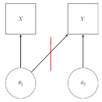
Figure 1: Graphical structure of the two-module system. The dashed line indicates the cut.

As shown in Carmona and Nicholls (2020) and Nicholls et al. (2022a), the cut posterior is a “generalized” posterior distribution (see, e.g., Bissiri et al., 2016) that restricts the information flow to guard against model misspecification (Frazier and Nott, 2022). In the canonical two module system, the cut posterior takes the form

$$\pi_{\mathrm{cut}}(\theta\mid Z):=\pi_{\mathrm{cut}}(\theta_{1}\mid X)\pi(\theta_{2}\mid Y,\theta_{1}),\quad\pi_{\mathrm{cut}}(\theta_{1}\mid X)\propto f_{1}(X\mid\theta_{1})\pi(\theta_{1}).$$

The common argument given for the use of $\pi_{\mathrm{cut}}(\theta\mid Z)$ instead of $\pi(\theta\mid Z)$ is the belief that misspecification adversely impacts inferences for $\theta_{1}$; e.g., Liu et al. (2009), and Jacob et al. (2017). The cut posterior uses only information from the data $X$ in making inference about $\theta_{1}$, ensuring our inference is insensitive to misspecification of the model for $Y$. However, uncertainty about $\theta_{1}$ can still be propagated through for inference on $\theta_{2}$ via the conditional posterior $\pi(\theta_{2}\mid\theta_{1},Y)$.

Motivating example: HPV prevalence and cervical cancer incidence

We now discuss a simple example described in Plummer (2015) that illustrates some of the benefits of cut model inference. The example, which we will return to in Section 4.3, is based on data from a real epidemiological study (Maucort-Boulch et al., 2008). Of interest is the international correlation between high-risk human papillomavirus (HPV) prevalence and cervical cancer incidence, for women in a certain age group. There are two data sources. The first is survey data on HPV prevalence for 13 countries. There are $X_{i}$ women with high-risk HPV in a sample of size $n_{i}$ for country $i$, $i=1,\dots,13$. There is also data on cervical cancer incidence, with $Y_{i}$ cases in country $i$ in $T_{i}$ woman years of follow-up. The data are modelled as

$$X_{i}\sim\text{Binomial}(n_{i},\theta_{1,i}),\;\;\;i=1,\dots,13,$$

$$Y_{i}\sim\text{Poisson}(\lambda_{i}),\;\;\;\log\lambda_{i}=\log T_{i}+\theta_{2,1}+\theta_{2,2}\theta_{1,i}.$$

The prior for $\theta_{1}=(\theta_{1,1},\dots,\theta_{1,13})^{\top}$ assumes independent components with uniform marginals on $[0,1]$. The prior for $\theta_{2}=(\theta_{2,1},\theta_{2,2})^{\top}$, assumes independent normal components, $N(0,1000)$.

Module 1 consists of $\pi(\theta_{1})$ and $f(X\mid\theta_{1})$ (survey data module) and module 2 consists of $\pi(\theta_{2})$ and $f(Y\mid\theta_{2})$ (cancer incidence module). The Poisson regression in the second module is grossly misspecified. Because of the coupling of the survey and cancer incidence modules, with the HPV prevalence values $\theta_{1}^{i}$ appearing as covariates in the Poisson regression for cancer incidence, the cancer incidence module contributes misleading information about the HPV prevalence parameters. The cut posterior estimates these parameters based on the survey data only, preventing contamination of the estimates by the misspecified module. This in turn results in more interpretable estimates of the parameter $\theta_{2}$ in the misspecified module, since $\theta_{2}$ summarizes the relationship between HPV prevalence and cancer incidence, but the summary produced can only be useful when the inputs to the regression (i.e. the HPV prevalence covariate values) are properly estimated.

Figure 2 shows the marginal posterior distribution for $\theta_{2}$ for both the full and cut posterior distribution, which are very different, illustrating how the misspecification of the cancer incidence module distorts inference about HPV prevalence in the full posterior, resulting in uninterpretable estimation for $\theta_{2}$. We will return to this example in Section 5, where we show the benefits of a semi-modular inference approach in which the tuning parameter $\omega$ interpolating between the cut and full posterior can be chosen based on a user-defined loss function reflecting the purpose of the analysis.

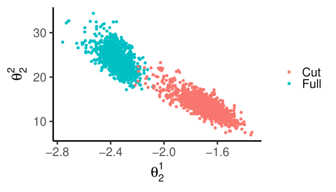
Figure 2: Marginal full and cut posterior distributions for $\theta_{2}$ in the HPV example.

2.2 Local misspecification framework

Throughout the remainder, we consider a slight generalisation of the canonical two-module system and assume that the modules are such that the joint likelihood takes the form

$$f(Z\mid\theta)\propto f_{1}(Z\mid\theta_{1})f_{2}(Z\mid\theta_{1},\theta_{2}),$$

where the individual models may or may not depend on the joint data $Z$. In the expressions above, the terms $f_{1}(Z\mid\theta_{1})$ and $f_{2}(Z\mid\theta_{1},\theta_{2})$ are not densities as functions of $Z$; these simply denote terms in a decomposition of the likelihood having the dependence indicated by the arguments. We furthermore suppose that the model $f_{1}(Z\mid\theta_{1})$ can identify $\theta_{1}$, but that the likelihood term $f_{2}(Z\mid\theta_{1},\theta_{2})$ contains additional information about $\theta_{1}$; see the regularity conditions in Appendix A for specific details. In this case, the cut posterior can be represented as follows:

$$\pi_{\mathrm{cut}}(\theta\mid Z):=\pi_{\mathrm{cut}}(\theta_{1}\mid Z)\pi(\theta_{2}\mid Z,\theta_{1}),\quad\pi_{\mathrm{cut}}(\theta_{1}\mid Z):=\frac{f_{1}(Z\mid\theta_{1})\pi(\theta_{1})}{\int_{\Theta}f_{1}(Z\mid\theta_{1})\pi(\theta_{1})\mathrm{d}\theta_{1}}.$$ (2)

The philosophy behind the use of the cut posterior inference is the belief that the misspecification ensures standard Bayesian inference (i.e., joint inference) results in “less accurate” results for $\theta_{1}$ than those obtained from the marginal model, $f_{1}(\cdot\mid\theta_{1})$, alone. In the definition of the cut posterior density (2), the marginal cut posterior density for $\theta_{1}$ is based on the first module only, whereas conditional inference for $\theta_{2}$ given $\theta_{1}$ is based on the second module only. In order to mathematically study the benefits of cut posterior inference compared to conventional Bayesian inference, we consider a setting where the data generating process (DGP) is locally misspecified in the following manner. The assumed model for the data has density

$$f(z\mid\theta)=f_{1}(z\mid\theta)f_{2}(z\mid\theta),$$

but the true DGP belongs to a family of distributions with density

$$h(z\mid\theta,\delta)=f_{1}(z\mid\theta)f_{2}(z\mid\theta,\delta),$$

where, in the nomenclature of Claeskens and Hjort (2003), $\delta\in\Delta\subseteq\mathbb{R}^{d_{\delta}}$ is an expansion parameter and is such that for some value for $\theta=(\theta_{1}^{\top},\theta_{2}^{\top})^{\top}$, denoted $\theta_{0}=(\theta_{1,0}^{\top},\theta_{2,0}^{\top})^{\top}$, we have $f_{2}(z\mid\theta_{0},\delta_{0})=f_{2}(z\mid\theta_{0})$, and $\theta_{0}$ corresponds to the “true” parameter value. We follow Claeskens and Hjort (2003) and consider a DGP that depends on a drifting sequence of values for $\delta$ depending on the sample size, and denoted by $\delta_{n}$, $n\geq 1$.

Assumption 1.

The observed data $\{Z_{i,n}:i\geq 1,n\geq 1\}$ is generated from an $n$-dependent stochastic process, such that, for fixed $n\geq 1$, $Z_{i,n}$ is independent and identically distributed according to the density function $h(z\mid\theta_{0},\delta_{n}):=f_{1}(z\mid\theta_{1,0})f_{2}(z\mid\theta_{0},\delta_{n})$, where $\delta_{n}:=\delta_{0}+\psi/\sqrt{n}$, with $\delta_{n}\in\Delta\subseteq\mathbb{R}^{d_{\delta}}$ for all $n\geq 1$. For all $z\in\mathcal{Z}$, excepting a set of measure zero, $h(z\mid\theta,\delta_{0})=f_{1}(z\mid\theta_{1})f_{2}(z\mid\theta)$.

In what follows, for any function $f:\mathcal{Z}\rightarrow\mathbb{R}^{d}$, we let $\mathbb{E}_{n}[f(Z)]$ denote the expectation of $f(Z)$ under $h(z\mid\theta_{0},\delta_{n})$ in Assumption 1; i.e., $\mathbb{E}_{n}[f(Z)]=\int_{\mathcal{Z}}f(z)h(z\mid\theta_{0},\delta_{n})\mathrm{d}\mu(z)$.

Remark 1.

Assumption 1 is similar to the misspecification device employed in Hjort and Claeskens (2003); Claeskens and Hjort (2003) to construct methods that combine, and choose between, different frequentist point estimators. Similar to their analysis, see, e.g., Section 2.1 in Hjort and Claeskens (2003), Assumption 1 creates a level of ambiguity as to whether or not the model is misspecified. This misspecification framework differs from the designs in Pompe and Jacob (2021), and Frazier and Nott (2022), where it is known with probability converging to one if the model is misspecified. The key feature of Assumption 1 is that the rate at which we learn about misspecification, $\sqrt{n}$, is the same rate with which sample information accumulates, ensuring that there is always a level of ambiguity regarding whether the model is correctly specified. This leads to theory which is practically useful for guiding a choice between cut and full posterior inference, since if there is no ambiguity regarding the existence of misspecification then the choice is obvious.

Under Assumption 1 and the standard regularity conditions given in Appendix A, we can deduce the asymptotic behavior of the exact posterior and its posterior mean. To state this result, we first require some definitions. Let $\ell(\theta)=\log f(Z\mid\theta)$ denote the joint log-likelihood, denote the full derivative of the log-likelihood as $\dot{\ell}(\theta):=\partial\ell(\theta)/\partial\theta$, and denote the second derivatives by $\ddot{\ell}(\theta):=\partial^{2}\ell(\theta)/\partial\theta\partial\theta^{\top}$. Likewise, define the matrix $\mathcal{I}=-\lim_{n}n^{-1}\mathbb{E}_{n}[\ddot{\ell}(\theta_{n})]$. Lastly, let $\eta:=\lim_{n}n^{-1}\mathbb{E}_{n}[\dot{\ell}_{i}(\theta_{0})\partial h(z_{i}\mid\theta_{0},\delta)/\partial\delta^{\top}|_{\delta=\delta_{n}}]\psi$, and partition $\eta$ conformably with $\theta=(\theta_{1}^{\top},\theta_{2}^{\top})^{\top}$ as $\eta=(\eta_{1}^{\top},\eta_{2}^{\top})^{\top}$.

Theorem 1.

If Assumption 1 and the regularity conditions in Appendix A are satisfied, then $\sqrt{n}\{\mathbb{E}_{\pi(\theta\mid Z)}(\theta)-\theta_{0}\}\Rightarrow N(\mathcal{I}^{-1}\eta,\mathcal{I}^{-1})$.

Theorem 1 demonstrates that, due to model misspecification in large samples the posterior behaves like the random variable

$$\theta_{0}+\mathcal{I}^{-1}\eta/\sqrt{n}+N(0,\mathcal{I}^{-1}/n).$$

Hence, the central posterior mass can deviate from $\theta_{0}$ depending on the magnitude of $\psi$, which encapsulates the “level” of model misspecification in Assumption 1, but the posterior variance is not impacted. Critically, both components of $\theta$ are impacted even though misspecification is confined to the second module.

Since cut posterior inferences for $\theta_{1}$ are not polluted by misspecification of the second module, we can expect that the behavior of $\pi_{\mathrm{cut}}(\theta_{1}\mid Z)$ will differ from that of $\pi(\theta_{1}\mid Z)$. To show such a result we require some additional notation. Firstly, consider that

$$\ell(\theta)=\log f_{1}(Z\mid\theta_{1})+\log f_{2}(Z\mid\theta)=\ell_{p}(\theta_{1})+\ell_{c}(\theta),$$

where $\ell_{p}(\theta_{1}):=\log f_{1}(Z\mid\theta_{1})$ signifies the ‘partial likelihood’ term, and $\ell_{c}(\theta):=\log f_{2}(Z\mid\theta_{1},\theta_{2})$ signifies the log-likelihood term that is used in cut inference to construct the conditional posterior. Define the partial derivatives $\dot{\ell}_{i(j)}=\partial\ell_{i}(\theta)/\partial\theta_{j}$, $\ddot{\ell}_{i(jk)}(\theta)=\partial^{2}\ell_{i(jk)}/\partial\theta_{j}\partial\theta_{k}^{\top}$, for $i\in\{p,c\}$, and $j\in\{1,2\}$. Let $\mathcal{I}_{i(jk)}=-\lim_{n}n^{-1}\mathbb{E}_{n}[\ddot{\ell}_{i(jk)}(\theta_{n})]$, $i\in\{p,c\}$, and $j,k\in\{1,2\}$.

Theorem 2.

If Assumption 1 and the regularity conditions in Appendix A are satisfied, then $\sqrt{n}\{\mathbb{E}_{\pi_{\mathrm{cut}}(\theta_{1}\mid Z)}(\theta_{1})-\theta_{1,0}\}\Rightarrow N(0,\mathcal{I}^{-1}_{p(11)}).$

Theorem 2 demonstrates that the cut posterior for $\theta_{1}$ delivers robust, but inefficient point inferences for $\theta_{1,0}$. The implication of Theorems 1 and 2 is that we are faced with a bias-variance trade-off when choosing between cut or exact posterior inferences for $\theta_{1,0}$: cut posterior point inferences are asymptotically unbiased, but have larger variance than under the exact posterior, which exhibits asymptotic bias. While the existence of a bias-variance trade-off has been a key tenet behind the exploration and analysis of cutting feedback methods, the above results constitute the first formalisation of this trade-off.

3 Semi-Modular Inference

Theorems 1-2 clarify that we face a trade-off when deciding whether to base inferences on the cut or exact posteriors. An approach that may be able to leverage this trade-off is semi-modular inference (SMI), which was initially proposed in Carmona and Nicholls (2020). SMI proposes to produce inferences for $\theta$ by interpolating between the exact and cut posteriors.

However, there are many ways to interpolate two probability distributions, and there is no a priori reason to suspect one method of interpolation will deliver better results than others. See Nicholls et al. (2022a) for a discussion on some of the possibilities. A common approach for combining probability distributions is linear opinion pools (Stone, 1961). Using a linear opinion pool one can construct a semi-modular posterior (SMP) as a convex combination of the exact and cut posterior distributions:

$$\pi_{\omega}(\theta\mid Z) :=\pi_{\omega}(\theta_{1}\mid Z)\pi(\theta_{2}\mid Z,\theta_{1}),$$ (3)

$$\pi_{\omega}(\theta_{1}\mid Z) :=(1-\omega)\pi_{\mathrm{cut}}(\theta_{1}\mid Z)+\omega\pi(\theta_{1}\mid Z).$$

In the case of modular inference based on intractable likelihoods, Chakraborty et al. (2022) suggest producing a linear opinion pool between the cut and exact posteriors based on summary statistics. However, to choose the value of $\omega$ the authors follow Yu et al. (2023) and consider prior-predictive conflict checks. Here we will consider an alternative approach and develop theoretical support for this approach, which the approach of Chakraborty et al. (2022) lacks. In what follows we restrict our attention to the SMP in (3), and leave a similar analysis for other constructions of the SMP for future research.

3.1 A Generalized Semi-modular Posterior

The SMP in (3) will allows us to explicitly leverage the bias-variance trade-off between the exact and cut posteriors (Theorems 1-2), and ultimately produce a novel SMP that is more accurate than using either posterior by itself, at least for $\theta_{1}$. To motivate our SMP, consider the pooled posterior in (3), with generic weight $\omega\in[0,1]$, and its corresponding point estimator of $\theta_{1,0}$

$$\overline{\theta}_{1}(\omega) :=(1-\omega)\int\theta_{1}\pi_{\mathrm{cut}}(\theta_{1}\mid Z)\mathrm{d}\theta_{1}+\omega\int\theta_{1}\pi(\theta_{1}\mid Z)\mathrm{d}\theta_{1}$$

$$=\overline{\theta}_{1,\mathrm{cut}}-\omega(\overline{\theta}_{1,\mathrm{cut}}-\overline{\theta}_{1,\mathrm{exact}}),$$

where $\overline{\theta}_{1,\mathrm{cut}}:=\int_{\Theta_{1}}\theta_{1}\pi_{\mathrm{cut}}(\theta_{1}\mid Z)\mathrm{d}\theta_{1}$ is the cut posterior mean, and $\overline{\theta}_{1,\mathrm{exact}}:=\int_{\Theta}\theta_{1}\pi(\theta_{1},\theta_{2}\mid Z)\mathrm{d}\theta$ is the exact posterior mean.

Under the results of Theorems 1 and 2, the asymptotic mean of $\sqrt{n}(\overline{\theta}_{1,\mathrm{cut}}-\theta_{0})$ is zero, while that of $\sqrt{n}(\overline{\theta}_{1,\mathrm{exact}}-\theta_{1,0})$ is $\eta_{1}$. Further, consider the simplified case where the variances of these estimators are $\tau^{2}\mathrm{I}_{d_{1}}$, and $\sigma^{2}\mathrm{I}_{d_{1}}$, $\sigma^{2}\leq\tau^{2}$, respectively, and where the two posterior means are asymptotically uncorrelated, so that $\text{Cov}\{\sqrt{n}(\overline{\theta}_{1,\mathrm{cut}}-\theta_{1,0}),\sqrt{n}(\overline{\theta}_{1,\mathrm{exact}}-\theta_{1,0})\}=0$ for all $n$. Extensions to more realistic cases are considered later. For some $\gamma>0$, if we take as our pooling weight

$$\widehat{\omega}=\min\left\{1,\frac{\gamma}{\|\widehat{\theta}_{1,\mathrm{cut}}-\widehat{\theta}_{1,\mathrm{exact}}\|^{2}}\right\},$$

we can investigate the asymptotic risk of the SMP based on $\widehat{\omega}$. The following result demonstrates that if we take $\omega=\widehat{\omega}$, then the asymptotic risk of the SMP in (3) is smaller than that of the cut posterior.

Lemma 1.

Assume that $\sqrt{n}(\overline{\theta}_{1,\mathrm{cut}}-\theta_{1,0})\Rightarrow N(0,\tau^{2}I)$ and $\sqrt{n}(\overline{\theta}_{1,\mathrm{exact}}-\theta_{1,0})\Rightarrow N(\eta_{1},\sigma^{2}I)$, and that $\mathrm{Cov}\{\sqrt{n}(\overline{\theta}_{1,\mathrm{cut}}-\theta_{1,0}),\sqrt{n}(\overline{\theta}_{1,\mathrm{exact}}-\theta_{1,0})\}=0$. If $d_{1}>2$, then for any $0<\gamma\leq 2(d_{1}-2)$,

$$\lim_{\nu\rightarrow\infty}\lim_{n\rightarrow\infty}\mathbb{E}_{n}\min[\|\sqrt{n}\{\overline{\theta}_{1}(\widehat{\omega})-\theta_{1,0}\}\|^{2},\nu] \leq d_{1}\tau^{2}-\frac{\gamma\tau^{4}\{2(d_{1}-2)-\gamma\}}{\eta_{1}^{\top}\eta_{1}+d_{1}\left(\sigma^{2}+\tau^{2}\right)}.$$

Lemma 1 demonstrates that, at least in simple settings, the risk of the cut posterior (given by $d_{1}\tau^{2}$) dominates the risk of the SMP constructed using $\widehat{\omega}$. The pooling weight $\widehat{\omega}$ resembles those used in the literature on shrinkage estimation, and in particular the shrinkage estimator proposed in Green and Strawderman (1991). While helpful to clarify the performance gains that may be achievable when using a SMP, this result is not applicable in general due to its strong assumptions. While a more general version of Lemma 1 can be established, which provides guarantees on the performance of our SMP in more realistic settings, before stating such a result we examine the above SMP based on $\widehat{\omega}$ in a simple example often used in the cutting feedback literature.

Example: Multivariate Biased Mean

To demonstrate the benefits of the SMP based on the above weighting scheme, we consider a slight modification of the biased mean example in Section 2.1 of Liu et al. (2009). Namely, we observe two datasets generated from independent random variables $Y_{1}$ and $Y_{2}$ with the same unknown mean $\theta_{1}$. However, the dataset for $Y_{2}$ is suspected to contain some unknown bias. Rather than attempting to conduct inference on this bias, as in Liu et al. (2009), we simply allow the SMP to interpolate between the cut and full posterior for $\theta_{1}$.

In particular, we observe two different datasets. The first dataset corresponds to $n_{1}$ observations on a $(d_{1}\times 1)$-dimensional random vector:

$$y_{1,i}=\theta_{1}+\epsilon_{1,i},$$

where $\theta_{1}=(\theta_{1,1},\dots,\theta_{1,d_{1}})^{\top}$ and $\epsilon_{1,i}$, $i=1,\dots,n_{1}$ are iid $N(0,I_{d_{1}})$. However, we also observe an additional dataset, comprised of $n_{2}>n_{1}$ observations that may be contaminated with bias, and whose scale is unknown,

$$y_{2,i}=\theta_{1}+\sigma\epsilon_{2,i},$$

where $\epsilon_{2,i}$, $i=1,\dots,n_{2}$ are iid $N(0,I_{d_{1}})$. Our priors are given as $\theta_{1}\sim N(0,\mathrm{I}_{d_{1}})$ and $\theta_{2}:=\sigma^{2}\propto 1/\sigma^{2}$. Our parameter of interest is $\theta_{1}$, and we wish to determine how much the second biased dataset should influence inference about $\theta_{1}$.

Suppose the second dataset is contaminated with bias for each component of $\theta_{1}$ independently, which results from contamination of the error term $\epsilon_{2,i}$, so that the actual distribution of $\epsilon_{2,i}$ is not $N(0,I_{d_{1}})$ but

$$\epsilon_{2,i}\stackrel{{\scriptstyle iid}}{{\sim}}\begin{cases}N(-0.25\cdot I_{d_{1}},0.1^{2}\cdot I_{d_{1}})&\text{ with prob. }\delta\\ N(0,\sigma^{2}I_{d_{1}})&\text{ with prob. }1-\delta\end{cases}$$

and where $\sigma^{2}=1/2$. For our experiments, we use an equally spaced grid of values for the contamination $\delta\in\{0:0.05:0.9\}$. For each value in this grid, we generate 1000 replications from the above process in the case where $n_{1}=100$ and $n_{2}=1000$. For each dataset, we apply the cut, exact, and SMP $\pi_{\widehat{\omega}}(\theta\mid Z)$ based on the weight

$$\widehat{\omega}=\min\left\{1,\frac{\mathrm{tr}[\text{Cov}_{\pi_{\mathrm{cut}}(\theta\mid Z)}(\theta_{1})]}{\|\overline{\theta}_{1,\mathrm{cut}}-\overline{\theta}_{1,\mathrm{exact}}\|^{2}}\right\}.$$

We then calculate the risk for each method and plot the averages across the replications in Figure 3, which considers $d_{1}=1$ and $d_{1}=5$ for the dimension of $\theta_{1}$, respectively.

Analyzing the results in Figure 3, we see that for relatively small values of the contamination, the exact posterior (represented by ‘Exact’ in the plot) has lower risk than the cut posterior, due to the much smaller variance, while at higher levels of contamination the cut posterior has lower risk. However, the risk of the proposed SMP is always (weakly) lower than both the exact and cut posteriors, which demonstrates that the SMP is able to ‘trade-off’ between the two posteriors so as to minimize risk across all levels of contamination. Consequently, at least in terms of risk the SMP is (weakly) preferable to both estimators across all levels of contamination.

Figure 3: Monte Carlo risk approximation across different levels of contamination ($\delta_{n}$). Exact refers to the risk for $\theta_{1,0}$ associated with the exact posterior based on both sets of data; Cut is the risk associated to the cut posterior; SMP is the risk for the proposed semi-modular posterior.

4 Risk Analysis

We now analyse the accuracy of the proposed SMP under the framework of asymptotic risk under weaker assumptions than those considered in previous section.

4.1 Measuring Accuracy via Risk

Rather than focusing on a predictive accuracy criterion, as in Carmona and Nicholls (2020), we propose that the researcher should choose the weighting in the SMP to produce accurate inferences on the precise quantity they wish to conduct inference on, and to measure the accuracy of this quantity relative to the loss function that is best suited to their analysis. To this end, we assume that the quantity of interest can be expressed as the unknown parameter $\beta_{0}=g(\theta_{1,0})\in\mathcal{B}$, which depends on the true unknown parameters $\theta_{1,0}$. For $B:=\{B_{n}\in\mathcal{B}:n\geq 1\}$ denoting a sequence of estimators for $\beta_{0}$, we assume that the researcher wishes to measure the accuracy with which $B_{n}$ estimates $\beta_{0}$ using a loss function $q:\mathcal{B}\times\mathcal{B}\rightarrow\mathbb{R}_{+}$ that satisfies the following assumptions.

Assumption 2.

For all $\beta,B\in\mathcal{B}$, the loss function $q(\beta,B)$ satisfies: i) $q(\beta,B)\geq 0$; ii) $q(\beta,\beta)=0$; iii) $\Upsilon(\beta)=\partial^{2}q(\beta,B)/\partial B\partial B^{\top}|_{B=\beta}$ is continuous, and semi-definite, in a neighbourhood of $\beta_{0}$, and $\Upsilon(\beta_{0})$ is positive-definite.

The accuracy of the estimator $B_{n}$ can then be measured via the trimmed expected loss, under $\theta_{n}$,

$$\mathcal{R}(\beta_{0},B_{n};\nu)=\mathbb{E}_{n}\min\left\{n\cdot q(\beta_{0},B_{n}),\nu\right\};$$

hereafter, we refer to $\mathcal{R}(\beta_{0},B_{n};\nu)$ simply as risk, or trimmed risk when we wish to emphasize the trimming. The risk $\mathcal{R}(\beta_{0},B_{n};\nu)$ is infeasible to evaluate in general, and may not even exist in finite samples, since $B_{n}$ may not have sufficient moments in finite samples. Hence, we use a closely related theoretical counterpart to measure the accuracy of $B_{n}$; namely, the asymptotic trimmed risk. We abuse notation and define the asymptotic expected risk for the sequence $\{B_{n}:n\geq 1\}$ as

$$\mathcal{R}_{0}(B_{n}):=\lim_{\nu\rightarrow\infty}\liminf_{n\rightarrow\infty}\mathcal{R}(\beta_{0},B_{n};\nu).$$ (4)

This choice of accuracy measure is commonplace for such analysis, see, e.g., Chapter 6 of Lehmann and Casella (2006), but is also feasible to calculate so long as $B_{n}$ has a tractable limiting distribution. Further, we note that the choice of $\beta$ and $q(\cdot)$ allows the user to define the features of interest for the inference problem, and hence to choose an estimator (or posterior in our case) that is accurate according to a measure appropriate for the problem at hand.

In general, so long as $g(\cdot)$ is a continuously differentiable function, and if we restrict the analysis to point estimators $\widehat{\vartheta}_{1}$ that are $\sqrt{n}$-consistent, under Assumption 2 we can immediately transfer results on the risk of an estimator of $\theta_{1,0}$ to $\beta_{0}$ (via the continuous mapping theorem). This follows since under this case, the loss function $q\{\beta_{0},g(\widehat{\vartheta}_{1})\}$ can asymptotically be represented as a weighted quadratic form in $(\widehat{\vartheta}_{1}-\theta_{1,0})$ that depends on the matrix $\Upsilon(\beta_{0})$. Hence, since both $\overline{\theta}_{\mathrm{cut}}$ and $\overline{\theta}_{\mathrm{exact}}$ are $\sqrt{n}$-consistent for $\theta_{0}$, throughout the remainder we consider the case where $g(\cdot)$ is the identify function.

4.2 Risk for $\theta_{1,0}$

Following the analysis in Section 3.1, we suggest to choose the weight in our SMP as the value of $\omega$ that minimises the asymptotic risk of $\overline{\theta}_{1}(\omega)$. The following result demonstrates that the value of $\omega$ that minimizes the limiting trimmed risk $\mathcal{R}_{0}\{\overline{\theta}_{1}(\omega)\}$ has a relatively simple closed form; to state this result, recall that, from the notations in Section 2.2, $\mathcal{I}_{(jk)}:=-\lim_{n}n^{-1}\mathbb{E}_{n}[\ddot{\ell}_{(jk)}(\theta_{0})]$, and define $\mathcal{I}_{(ii.j)}:=\mathcal{I}_{(ii)}-\mathcal{I}_{(ij)}\mathcal{I}_{(jj)}^{-1}\mathcal{I}_{(ji)}$; further, for $i\in\{p,c\}$, let $\mathcal{I}_{i(jk)}:=-\lim_{n}n^{-1}\mathbb{E}_{n}[\ddot{\ell}_{i(jk)}(\theta_{0})]$, where $\ddot{\ell}_{i(jk)}(\theta_{n})=\partial^{2}\ell_{i}(\theta)/\partial\theta_{j}\partial\theta_{k}^{\top}$, $j,k\in\{1,2\}$, and where we recall that $\ell_{p}(\theta_{1})=\log f_{1}(Z\mid\theta_{1})$ and $\ell_{c}(\theta)=\log f_{2}(Z\mid\theta)$.

Lemma 2.

Suppose that Assumptions 1-2 and the regularity conditions in Appendix A are satisfied, and let $\Upsilon=\Upsilon(\theta_{1,0})$. Then, $\mathcal{R}_{0}\{\overline{\theta}_{1}(\omega)\}$ is minimized at

$$\omega^{\star}=\begin{cases}\frac{\mathrm{tr}\Upsilon(\mathcal{I}_{p(11)}^{-1}-\mathcal{I}_{11.2}^{-1})}{\left(\eta_{1}-\mathcal{I}_{12}\mathcal{I}_{22}^{-1}\eta_{2}\right)^{\top}\mathcal{I}_{11.2}^{-1}\Upsilon\mathcal{I}_{11.2}^{-1}\left(\eta_{1}-\mathcal{I}_{12}\mathcal{I}_{22}^{-1}\eta_{2}\right)+\mathrm{tr}\Upsilon(\mathcal{I}_{p(11)}^{-1}-\mathcal{I}_{11.2}^{-1})}&\mathrm{if}\;\mathrm{tr}\Upsilon(\mathcal{I}_{p(11)}^{-1}-\mathcal{I}_{11.2}^{-1})>0\\ 0&\mathrm{otherwise}\end{cases}.$$

Analysing the above form of $\omega^{\star}$, each of the above pieces can be consistently estimated from the posteriors, except for $\eta_{1}$. However, following the discussion in Section 3.1, and in particular the result of Lemma 1, we can employ $n\{\overline{\theta}_{1,\mathrm{cut}}-\overline{\theta}_{1,\mathrm{exact}}\}^{\top}\widehat{\Upsilon}\{\overline{\theta}_{1,\mathrm{cut}}-\overline{\theta}_{1,\mathrm{exact}}\}$, where $\widehat{\Upsilon}=\Upsilon\ (\overline{\theta}_{1,\mathrm{exact}})$, as an estimator for the denominator in $\omega^{\star}$.

With reference to Lemma 1, this then suggests the following mixing weight $\widehat{\omega}_{+}:=\min\{1,\widehat{\omega}\}$ for the SMP, where, for a user-chosen shrinkage parameter sequence $\gamma_{n}\rightarrow_{p}\gamma$, and $\gamma>0$,

$$\widehat{\omega}=\frac{\gamma_{n}}{n(\overline{\theta}_{1,\mathrm{cut}}-\overline{\theta}_{1,\mathrm{exact}})^{\top}\widehat{\Upsilon}(\overline{\theta}_{1,\mathrm{cut}}-\overline{\theta}_{1,\mathrm{exact}})}.$$

Taking $\omega=\widehat{\omega}_{+}$ for the SMP in (3) yields the SMP

$$\pi_{\widehat{\omega}_{+}}(\theta\mid Z):=\{(1-\widehat{\omega}_{+})\pi_{\mathrm{cut}}(\theta_{1}\mid Z)+\widehat{\omega}_{+}\pi(\theta_{1}\mid Z)\}\pi(\theta_{2}\mid\theta_{1},Z)$$ (5)

which is parameterized in terms of the user-chosen sequence $\gamma_{n}$. Letting $W=\Upsilon(\mathcal{I}_{p(11)}^{-1}-\mathcal{I}_{11.2}^{-1})$, we can then obtain the following result on the risk associated with the SMP.

Corollary 1.

Consider that Assumptions 1-2, and the regularity conditions in Appendix A are satisfied. If $\mathrm{tr}W-2\|W\|>0$, and $0<\gamma<2(\mathrm{tr}W-2\|W\|)$, then for any $\eta_{1}\in\Theta_{1}$,

$$\mathcal{R}_{0}(\overline{\theta}_{1,+})<\mathcal{R}_{0}(\overline{\theta}_{1,\mathrm{cut}}).$$

Furthermore, if $\left(\eta_{1}-\mathcal{I}_{12}\mathcal{I}_{22}^{-1}\eta_{2}\right)^{\top}\mathcal{I}_{11.2}^{-1}\Upsilon\mathcal{I}_{11.2}^{-1}\left(\eta_{1}-\mathcal{I}_{12}\mathcal{I}_{22}^{-1}\eta_{2}\right)\geq\mathrm{tr}W,$ then

$$\mathcal{R}_{0}(\overline{\theta}_{1,+})<\mathcal{R}_{0}(\overline{\theta}_{1,\mathrm{exact}}).$$

The first part of Corollary 1 demonstrates that a sufficient condition for $\mathcal{R}_{0}(\overline{\theta}_{1,+})<\mathcal{R}_{0}(\overline{\theta}_{1,\mathrm{cut}})$ is that there is a sufficient reduction in uncertainty for inference conducted under the exact posteriors relative to the cut posterior. Indeed, the larger is $\mathrm{tr}W-2\|W\|$, which is related to the magnitude of $\mathcal{I}_{p(11)}^{-1}-\mathcal{I}_{11.2}^{-1}$, the larger is the gap between the risk of the SMP and the cut posteriors. Further, the above result applies even if $\eta=0$, i.e., even when there is no asymptotic bias for inferences conducted under the exact posterior. In this way, so long as $\mathrm{tr}W>2\|W\|$, Corollary 1 demonstrates that there are always inferential gains to be had by using the SMP over the cut posterior.

The second part of Corollary 1 gives a sufficient, but not necessary, condition which guarantees that the risk associated with $\pi(\theta_{1}\mid Z)$ dominates that of our SMP $\pi_{\widehat{\omega}_{+}}(\theta_{1}\mid Z)$. This condition is likely to be satisfied when the difference in posterior locations, captured via $\tau^{\top}(\Gamma_{1}-\Gamma)^{\top}\Upsilon(\Gamma_{1}-\Gamma)\tau$, is large relative to the difference in the posterior variances, measured by $\mathrm{tr}W=\mathrm{tr}\Upsilon(\mathcal{I}_{p(11)}^{-1}-\mathcal{I}_{11.2})$. We also note that the results in Corollary 1 are valid across a wide range of user-chosen shrinkage sequences $\gamma_{n}$, so long as its limit $\gamma$ satisfies the condition that $0\leq\gamma\leq 2(\mathrm{tr}W-2\|W\|)$.

We show in Theorem 3 in Appendix C that the risk for the SMP is minimized at ${\gamma}=\mathrm{tr}W-2\|W\|$. A convenient estimator of $\gamma$ is then to take $\widehat{\mathcal{I}}_{p(11)}^{-1}=\text{Cov}_{\pi_{\mathrm{cut}}(\theta_{1}\mid Z)}(\theta_{1})$, $\widehat{\mathcal{I}}_{11.2}^{-1}=\text{Cov}_{\pi(\theta_{1}\mid Z)}(\theta_{1})$, and set $\gamma=\widehat{\gamma}$, where

$$\widehat{\gamma}=\mathrm{tr}\widehat{\Upsilon}(\widehat{\mathcal{I}}_{p(11)}^{-1}-\widehat{\mathcal{I}}_{11.2}^{-1})-2\|\widehat{\Upsilon}(\widehat{\mathcal{I}}_{p(11)}^{-1}-\widehat{\mathcal{I}}_{11.2}^{-1})\|.$$ (6)

Furthermore, Theorem 3 in Appendix C yields an exact result for the risk when $\Upsilon=(\mathcal{I}_{p(11)}^{-1}-\mathcal{I}_{11.2})^{-1}$.

Corollary 2.

Consider that Assumptions 1-2, and the regularity conditions in Appendix A are satisfied. If $\Upsilon=({\mathcal{I}}_{p(11)}^{-1}-{\mathcal{I}}_{11.2})^{-1}$, $d_{1}>2$, and $0<\gamma<2(d_{1}-2)$, then for any $\eta\in\Theta$, such that $\left(\eta_{1}-\mathcal{I}_{12}\mathcal{I}_{22}^{-1}\eta_{2}\right)^{\top}\mathcal{I}_{11.2}^{-1}\Upsilon\mathcal{I}_{11.2}^{-1}\left(\eta_{1}-\mathcal{I}_{12}\mathcal{I}_{22}^{-1}\eta_{2}\right)<\infty$,

$$\mathcal{R}_{0}(\overline{\theta}_{1,+}) =\mathcal{R}_{0}(\overline{\theta}_{1,\mathrm{cut}})-\frac{\gamma\{2(d_{1}-2)-\gamma\}(d_{1}-3)!}{2(d_{1})!}{{}_{1}F_{1}(d_{1}-1;d_{1};\lambda)}<\mathcal{R}_{0}(\overline{\theta}_{1,\mathrm{cut}}),$$

where ${{}_{1}F_{1}(k-1;k;\lambda)}$ is the confluent hyper-geometric function.

Remark 2.

Under $\Upsilon=(\mathcal{I}_{p(11)}^{-1}-\mathcal{I}_{11.2})^{-1}$, the condition $d_{1}>2$ is necessary to guarantee that $\pi_{\widehat{\omega}_{+}}(\theta_{1}\mid Z)$ has smaller risk than $\pi_{\mathrm{cut}}(\theta_{1}\mid Z)$. This condition is intimately related to James-Stein estimation and Stein’s paradox (see Ch. 6 of Lehmann and Casella, 2006 for a discussion), and ensures that a type of Stein phenomena exists in this case, which we can interpret as saying that the use of the cut posterior by itself is sub-optimal when $d_{1}\geq 3$. However, we stress that this interpretation is only valid in the case where $\Upsilon=(\mathcal{I}_{p(11)}^{-1}-\mathcal{I}_{11.2})^{-1}$ and a similar phenomena does not necessarily extend to other choices of the loss function. We also remark that the result of Corollary 1 does not require that $d_{1}>2$, as is the case for Corollary 2.

Together, Corollaries 1-2 demonstrate that the SMP can seamlessly weights the exact and cut posteriors in such a way that it will always yield more accurate inferences than using the cut posterior by itself. The theoretical results also demonstrate that if one chooses the weight in the SMP as in equation (6), then when there is little difference between the posterior locations of $\pi(\theta_{1}\mid Z)$ and $\pi_{\mathrm{cut}}(\theta_{1}\mid Z)$, the weight will be close to unity, and the SMP will resemble the exact posterior. However, Corollary 1 also shows that in cases where the locations of the cut and exact posterior disagree the risk of the SMP will be dominated by that of the exact posterior, i.e., $\mathcal{R}_{0}(\overline{\theta}_{1,+})<\mathcal{R}_{0}(\overline{\theta}_{1,\mathrm{exact}})$.

5 Examples

In this section, we apply the optimally weighted SMP derived in Section 2.2 to two examples encountered in the literature on cut model inference.

5.1 Normal-normal random effects model

We now apply the SMP to the misspecified normal-normal random effects model presented in Liu et al. (2009). The observed data is $Z_{ij}$ comprising observations on $i=1,\dots,N$ groups, with $j=1,\dots,J$ observations in each group, which we assume are generated from the model $Z_{ij}\mid\beta_{i},\varphi_{i}^{2}\stackrel{{\scriptstyle iid}}{{\sim}}N(\beta_{i},\varphi_{i}^{2})$, with random effects $\beta_{i}\mid\psi\stackrel{{\scriptstyle iid}}{{\sim}}N(0,\psi^{2})$. The goal of the analysis is to conduct inference on the standard deviation of the random effects, $\psi$, and the residual standard deviation parameters $\varphi=(\varphi_{1},\dots,\varphi_{N})^{\top}$. Below we write $\beta=(\beta_{1},\dots,\beta_{N})^{\top}$, and $\zeta=(\psi,\beta^{\top})^{\top}$.

For $\bar{Z}_{i}=J^{-1}\sum_{j=1}^{J}Z_{ij}$ and $s_{i}^{2}=\sum_{j=1}^{J}(Z_{ij}-\bar{Z}_{i})^{2}$, $i=1,\dots,N$, the likelihood for $\zeta,\varphi$ can be written to depend only on the sufficient statistics $\bar{Z}=(\bar{Z}_{1},\dots,\bar{Z}_{N})^{\top}$ and $s^{2}=(s_{1}^{2},\dots,s_{N}^{2})^{\top}$, where independently for $i=1,\dots,N$,

$$\bar{Z}_{i}\mid\zeta,\varphi\sim N(\beta_{i},\varphi_{i}^{2}/J),$$

$$s^{2}_{i}\mid\varphi\sim\text{Gamma}\left(\frac{J-1}{2},\frac{1}{2}\frac{1}{\varphi_{i}^{2}}\right).$$

Letting $\theta_{1}=\varphi$ and $\theta_{2}=\zeta$, the random effects model can then be written as a two-module system of the form shown in Figure 1: module one depends on $(s^{2},\theta_{1})$, $X=s^{2}$, and module two depends on $(\bar{Z},\theta_{2},\theta_{1})$, $Y=\bar{Z}$.

Let $\text{Gamma}(x;A,B)$ denote the value of the $\text{Gamma}(A,B)$ density evaluated at $x$, and $N(x;\mu,\sigma^{2})$ denote the value of the $N(\mu,\sigma^{2})$ density evaluated at $x$. The first module has likelihood $f_{1}(X\mid\theta_{1})=\prod_{i=1}^{N}\text{Gamma}\left(s_{i}^{2};\frac{J-1}{2},\frac{1}{2}\frac{1}{\theta_{1,i}^{2}}\right)$, while the second module has likelihood $f_{2}(Y\mid\theta)=\prod_{i=1}^{N}N(\bar{Z}_{i};\beta_{i},\theta_{1,i}^{2}/J)$.

When the Gaussian prior for the random effects term $\beta_{i}$ conflicts with the likelihood information, inferences for $\theta_{1,i}=\varphi_{i}$ can be adversely impacted. Such an outcome will happen when, for instance, a value of $\beta_{i}$ is much larger than the remaining components, and as shown in Liu et al. (2009), the resulting thin-tailed Gaussian assumption for the random effects may produce poor inference for $\theta_{1,i}$ due to the feedback induced by the likelihood term $N(\bar{Z}_{i};\beta_{i},\varphi_{i}^{2}/J)$ in the second module. Misspecification of the prior for the random effects can lead to exact inferences for $\theta_{1}$ that are substantially less accurate than those obtained under the cut posterior.

To guard against misspecification Liu et al. (2009) propose cut posterior inference for $\theta_{1}\mid s^{2}$, which can be accommodated by simply updating the posterior for $\theta_{1}$ using only the information in the corresponding summary statistics $s^{2}$: given $\pi(\theta_{1,i}^{2})\propto(\theta_{1,i}^{2})^{-1}$, and independent across $i=1,\dots,N$, the cut posterior for $\theta_{1}^{2}$ (where this denotes the elementwise square of $\theta_{1}$) is

$$\pi_{\mathrm{cut}}(\theta_{1}^{2}\mid X)\propto\prod_{i=1}^{N}(\theta_{1,i}^{2})^{-\frac{J+1}{2}}\exp\left\{-\frac{J\cdot s_{i}^{2}}{2\theta_{1,i}^{2}}\right\}.$$

Summaries of the cut posterior for $\theta_{1}$ can be obtained by sampling from the cut posterior for $\theta_{1}^{2}$ and transforming the samples. Joint inferences for $(\zeta,\varphi)$ can be carried out using the cut posterior distribution

$$\pi_{\mathrm{cut}}(\zeta,\varphi\mid X,Y) =\pi_{\mathrm{cut}}(\varphi\mid X)\pi(\zeta\mid Y,\varphi)=\pi_{\mathrm{cut}}(\varphi\mid s^{2})\pi(\zeta\mid\bar{Z},\varphi),\quad\varphi=\theta_{1},$$

where the conditional posterior $\pi(\zeta\mid\bar{Z},\varphi)$ is obtained from the joint posterior for $\theta_{1},\theta_{2}$.

We now demonstrate that the SMP proposed herein can seamlessly choose between the cut and exact posteriors to deliver posterior inferences for $\theta_{1}$ that are more accurate than either the exact or cut posteriors. To this end, we generate 1000 repeated samples from the normal-normal random effects model with $N=100$ groups and $J=10$ observations per-group. For each group we set $\theta_{1,i}:=\varphi_{i}=0.5$ and $\psi=1$. Following Liu et al. (2009) and Liu and Goudie (2022a), we induce model misspecification by setting a value for the random effect $\beta_{1}$ which is conflict with the prior, considering $\beta_{1}=X_{1}+\delta_{n}$, $X_{1}\sim N(0,1)$, with $\delta_{n}\in\{0.1,0.3,\dots,1.9\}$ across all replications. We then compare the behavior of the cut, exact and SMP for $\theta_{1,1}=\varphi_{1}$, where the posterior weight in the SMP is calculated using the estimator in equation (6).

We present the corresponding risk of the posteriors from the different procedures in Table 1. From the results of the table, we see that the SMP has superior performance to the cut or exact posterior in terms of risk. Across all values of $\delta_{n}$, the SMP has smaller risk than either the cut or exact posteriors, while the cut posterior is more accurate than the exact posterior in most cases.

$\delta_{n}$	$0.10$	$0.30$	$0.50$	$0.70$	$1.9$	$1.10$	$1.30$	$1.50$	$1.70$	$1.9$
$\mathrm{Cut}$	3.62	3.30	3.40	2.98	3.14	3.15	3.26	3.78	2.97	3.13
$\mathrm{Exact}$	3.67	3.29	3.39	2.97	3.16	3.22	3.31	3.89	3.05	3.19
$\mathrm{SMP}$	3.59	3.25	3.36	2.93	3.11	3.13	3.23	3.74	2.94	3.10

Table 1: Risk values, multiplied by 100, for readability. Bold values indicate the lowest value of risk across the methods.

5.2 HPV prevalence and cancer incidence: Revisited

We return to the example in Section 2.1, concerning the relationship between HPV prevalence and cervical cancer incidence. We use it to demonstrate how the semi-modular posterior can vary for different loss functions. In particular, we consider an SMP for a loss function targeting the HPV prevalence in country $j$, $\theta_{1,j}$, and show how the SMP mixing weight and semi-modular inferences vary across $j$. In the notation of Section 4.1, we choose $\beta=\theta_{1,j}$ and $q(\beta,T)=(\beta-T)^{2}$. We use the mixing weight

$$\widehat{\omega}=\frac{{\sigma_{\text{cut}}^{(j)}}^{2}-{\sigma^{(j)}}^{2}}{(\bar{\theta}_{1,\text{cut}}^{(j)}-\bar{\theta}_{1}^{(j)})^{2}},$$

where ${\sigma_{\text{cut}}^{(j)}}^{2}$ and ${\sigma^{(j)}}^{2}$ are the cut and full marginal posterior variances for $\theta_{1,j}$, and $\bar{\theta}_{1,\text{cut}}^{(j)}$ and $\bar{\theta}_{1}^{(j)}$ are the cut and full marginal posterior means. We denote the marginal SMP for $\theta_{1,j}$ by $\pi_{\text{cut}}^{(j)}(\theta_{1,j}|X)$, and Figure 4 shows kernel estimates of these densities together with the SMP mixing weights $\widehat{\omega}_{+}$, and the cut and full posterior $\theta_{1,j}$ marginals. The countries are ordered in the plot (left to right, top to bottom) according to the cut posterior mean values. The mixing weights vary widely according to the loss function used; when the difference in location of the cut and full posterior distributions is large compared to the posterior variability, the SMP is close to the cut posterior, whereas the SMP is closer to the full posterior otherwise. The strong dependence of the SMP on the loss function illustrates that it is important to consider the purpose of the analysis to obtain appropriate SMI inferences.

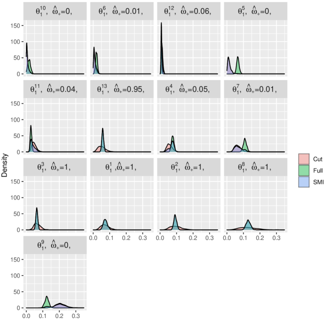
Figure 4: Marginal cut, full and semi-modular posterior (SMP) densities for HPV prevalence in different countries. The SMP obtained for country $j$ uses a loss function depending on $j$ as described in the text. $\hat{\omega}_{+}$ is the estimated mixing weight in the SMP. Countries are ordered (left to right, top to bottom) according to the cut posterior mean values.

MCMC computations for the full posterior distribution were done using Stan (Carpenter et al., 2017), whereas cut posterior samples for $\theta_{1}$ given $X$ are generated directly using conjugacy, followed by sampling importance resampling based on $1,000$ draws from an asymptotic normal approximation to the conditional posterior of $\theta_{2}$ given $\theta_{1}$, $Y$, to obtain each $\theta_{2}$ sample. Kernel density estimates in the plots are based on $1,000$ posterior samples.

6 Discussion

Choosing between the cut and full posterior distributions for inference can be difficult when model misspecification is not severe, and the semi-modular inference approach of Carmona and Nicholls (2020) is an attractive alternative to making a binary cut. The intuition behind the approach is based on a bias-variance trade-off, and this paper formalizes this trade-off for the first time in the literature. We further consider the SMP based on linear opinion pooling of Chakraborty et al. (2022), and develop a method for choosing the degree of influence parameter in this approach that has theoretical support, something which the SMP approaches of Chakraborty et al. (2022) and Carmona and Nicholls (2020) lack. A strength of our approach is that the construction of the SMP employs a user-defined loss function, which allows accurate estimation according to a criterion that reflects the problem at hand. Out theoretical results demonstrate that, under this loss function, our SMP delivers inferences that are superior to the cut and exact posterior under weak regularity conditions.

An interesting future direction would be to extend the theoretical results presented herein to alternative definitions of the SMP, both the original definition of Carmona and Nicholls (2020) and alternatives discussed more recently by Nicholls et al. (2022b). We note that since alternative SMPs have a different structure to that of the mixture SMP, the results obtained herein are not immediately applicable, and alternative arguments to those given here will be needed to deuce their theoretical behavior.

Appendix A Regularity Conditions

To formalize the impact of the misspecification in Assumption 1, we impose the following regularity conditions on the true density $h(z\mid\theta,\delta)$.

Assumption A1.

For $\zeta:=(\theta^{\top},\delta^{\top})^{\top}$, $\zeta_{0}:=(\theta_{0}^{\top},\delta_{0}^{\top})^{\top}$ is an element of the interior of $\Theta\times\Delta$, where $\Delta\subseteq\mathbb{R}^{d_{\delta}}$ is compact. The function $h(z\mid\zeta)$ is twice continuously differentiable for almost all $z\in\mathcal{Z}$. There exist positive functions $a(z)$, $b(z)$ such that for all $z_{i}\in\mathcal{Z}$, except on sets of measure zero, $\ell_{i}(\zeta)=\log h(z_{i}\mid\zeta)$, satisfies the following: $\exp\ell_{i}(\zeta)\leq a(z_{i})$, and for all $\|\zeta-\zeta_{0}\|\leq\nu/\sqrt{n}$, and some $\nu>0$, each of the following $|\ell_{i}(\zeta)|$, $\|\dot{\ell}_{i}(\zeta)\|^{2}$, $\|\ddot{\ell}_{i}(\zeta)\|^{2}$ are less than $b(z_{i})$. Further, $\mathbb{E}[a(z)],\mathbb{E}[b(z)]<+\infty$, and the set $\{z\in\mathcal{Z}:h(z\mid\zeta)>0\}$ does not depend on $\zeta$.

In addition, we maintain the following assumptions about the assumed model $f(z\mid\theta)$.

Assumption A2.

For $\ell_{i}(\theta)=\log f(z_{i}\mid\theta)$ the $i$-th likelihood increment, if $\theta\neq\theta_{0}$, then $\ell_{i}(\theta)\neq\ell_{i}(\theta_{0})$ with positive probability. The matrix $\lim_{n}n^{-1}\mathbb{E}_{n}\ddot{\ell}_{i}(\theta)$ exists, and is non-singular.

Remark 3.

Assumptions A1-A2 are standard in the classical literature on estimation of regular parametric models. Assumption A1 is similar to the regularity conditions employed by Claeskens and Hjort (2003) to deduce their large sample theory for their frequentist model averaging procedure, and give enough regularity to permit a second-order Taylor series expansion of $\ell_{i}(\zeta)$ around $\zeta_{0}$. Assumption A2 is a classical identification condition used for estimation of $\theta_{0}$.

The following condition is a standard regularity condition on the behavior of priors.

Assumption A3.

The prior density $\pi(\theta)$ is positive and continuous on $\Theta$, and $\int_{\Theta}\|\theta\|\pi(\theta)\mathrm{d}\theta<\infty$.

Appendix B Lemmas

The following intermediate results are used to help state and prove the main results of the paper.

Lemma B.1.

Consider that Assumptions 1, A1 and A2 are satisfied. Then, for any $\gamma\in\Delta$, the following results are satisfied.

1. $\lim_{n}n^{-1}\mathbb{E}_{n}[-\ddot{\ell}_{p(11)}(\theta_{1,0})]=\lim_{n}n^{-1}\mathbb{E}_{n}[\dot{\ell}_{p(1)}(\theta_{1,0})\dot{\ell}_{p(1)}(\theta_{1,0})^{\top}]$.

2. $\lim_{n}n^{-1}\mathbb{E}_{n}[-\ddot{\ell}_{c(11)}(\theta_{0})]=\lim_{n}n^{-1}\mathbb{E}_{n}[\dot{\ell}_{c(1)}(\theta_{0})\dot{\ell}_{c(1)}(\theta_{0})^{\top}]$.

3. $\lim_{n}n^{-1}\mathbb{E}_{n}[\dot{\ell}_{p(1)}(\theta_{1,0})\dot{\ell}_{c(1)}(\theta_{0})^{\top}]=0$.

4. $\lim_{n}n^{-1}\mathbb{E}_{n}[\dot{\ell}_{p(1)}(\theta_{1,0})\dot{\ell}_{c(2)}(\theta_{0})^{\top}]=0$.

Lemma B.2.

Consider that Assumptions 1, A1 and A2 are satisfied and let and $\eta=(\eta_{1}^{\top},\eta_{2}^{\top})^{\top}$ where

$$\eta_{1}:=\mathbb{E}\left[\frac{\partial\ell(\theta_{0})}{\partial\theta_{1}}\frac{\partial\log h(Z\mid\theta_{0},\delta_{0})}{\partial\delta^{\top}}\right]\psi,\quad\eta_{2}:=\mathbb{E}\left[\frac{\partial\ell(\theta_{0})}{\partial\theta_{2}}\frac{\partial\log h(Z\mid\theta_{0},\delta_{0})}{\partial\delta^{\top}}\right]\psi.$$

Then the following results are satisfied.

1. $\lim_{n}\mathbb{E}_{n}\left[\dot{\ell}(\theta_{0})/\sqrt{n}\right]=\eta$.

2. $\dot{\ell}(\theta_{0})/\sqrt{n}\Rightarrow N(\eta,\mathcal{I})$.

3. $\dot{\ell}_{p(1)}(\theta_{0})/\sqrt{n}\Rightarrow N(0,\mathcal{I}_{p(11)})$.

4. $\dot{\ell}_{c(2)}(\theta_{0})/\sqrt{n}\Rightarrow N(\eta_{2},\mathcal{I}_{c(22)}).$

To state the risk associated with this posterior in a simple form, we first give an intermediate result that describes the behavior of $\widehat{\omega}_{+}$ for arbitrary $\gamma$. To state the result, let $\mathbf{0}_{d_{1}\times d_{1}}$ denote a $d_{1}\times d_{1}$ matrix of zeros, $\Gamma_{1}:=(\mathcal{I}_{p(11)}^{-1}:\mathbf{0}_{d_{1}\times d_{1}}:\mathbf{0}_{d_{1}\times d_{2}})$, $\Gamma:=(\mathbf{0}_{d_{1}\times d_{1}}:\mathcal{I}_{11.2}^{-1}:-\mathcal{I}_{11.2}^{-1}\mathcal{I}_{12}\mathcal{I}_{22}^{-1})$, and

$$Z_{n}:=(\dot{\ell}_{p(1)}(\theta_{1,0})^{\top},\{\dot{\ell}_{p(1)}(\theta_{1,0})+\dot{\ell}_{c(1)}(\theta_{0})\}^{\top},\dot{\ell}_{c(2)}(\theta_{0})^{\top})^{\top}/\sqrt{n}.$$

Furthermore, let $\tau:=(\mathbf{0}_{d_{1}\times 1}:\eta^{\top})^{\top}$, and let $\xi:=(\xi_{1}^{\top},\xi_{2}^{\top},\xi_{3}^{\top})^{\top}$ denote a zero-mean normal vector with variance $\Omega:=\lim_{n}\mathbb{E}_{n}(Z_{n}Z_{n}^{\top})$, where $\xi_{1}$ and $\xi_{2}$ are both $(d_{1}\times 1)$-dimensional mean-zero Gaussian random variables, and $\xi_{3}$ is a $(d_{2}\times 1)$-dimensional mean-zero Gaussian random variable.

Lemma B.3.

Consider that Assumptions 1, A1 and A2 are satisfied. Then, $Z_{n}\Rightarrow\xi+\tau$, where $\tau=(\mathbf{0}_{d_{1}\times 1}^{\top},\eta^{\top})^{\top}$, and where $\xi$ is a $2d_{1}+d_{2}$ dimensional normal random variable with mean zero and variance matrix

$$\Omega:=\lim_{n\rightarrow+\infty}n^{-1}\begin{pmatrix}\mathbb{E}_{n}[\dot{\ell}_{p(1)}\dot{\ell}_{p(1)}^{\top}]&\mathbb{E}_{n}[\dot{\ell}_{p(1)}\dot{\ell}_{p(1)}^{\top}]&\mathbf{0}_{d_{1}\times d_{2}}\\ \mathbb{E}_{n}[\dot{\ell}_{p(1)}\dot{\ell}_{p(1)}^{\top}]&\mathbb{E}_{n}[\{\dot{\ell}_{p(1)}+\dot{\ell}_{c(1)}\}\{\dot{\ell}_{p(1)}+\dot{\ell}_{c(1)}\}^{\top}]&\mathbb{E}_{n}[\dot{\ell}_{c(1)}\dot{\ell}_{c(2)}^{\top}]\\ \mathbf{0}_{d_{2}\times d_{1}}&\mathbb{E}_{n}[\dot{\ell}_{c(2)}\dot{\ell}_{c(1)}^{\top}]&\mathbb{E}_{n}[\dot{\ell}_{c(2)}\dot{\ell}_{c(2)}^{\top}]\end{pmatrix}.$$

Furthermore, $(\Gamma_{1}-\Gamma)\Omega(\Gamma_{1}-\Gamma)^{\top}=\mathcal{I}_{p(11)}^{-1}-\mathcal{I}_{11.2}^{-1}$, and $\Gamma_{1}\Omega(\Gamma_{1}-\Gamma)^{\top}=-(\mathcal{I}_{p(11)}^{-1}-\mathcal{I}_{11.2}^{-1})$.

Using the above definitions, we can state the behavior of $\widehat{\omega}_{+}$, and the optimally weighted posterior mean combination

$$\overline{\theta}_{1,+}:=(1-\widehat{\omega}_{+})\overline{\theta}_{1,\mathrm{cut}}+\widehat{\omega}_{+}\overline{\theta}_{1,\mathrm{exact}}.$$

Lemma B.4.

Consider that Assumptions 1, and A1-A2 are satisfied. Then,

1. $\sqrt{n}\begin{pmatrix}\overline{\theta}_{1,\mathrm{cut}}-\theta_{1,0}\\ \overline{\theta}_{1,\mathrm{exact}}-\theta_{1,0}\end{pmatrix}=\begin{pmatrix}\Gamma_{1}\\ \Gamma\end{pmatrix}Z_{n}+o_{p}(1)\Rightarrow\begin{pmatrix}\Gamma_{1}\\ \Gamma\end{pmatrix}(\xi+\tau)$.

2. $\widehat{\omega}_{+}\Rightarrow\overline{\omega}:=\min\left\{1,\frac{\gamma}{(\xi+\tau)^{\top}(\Gamma_{1}-\Gamma)^{\top}\Upsilon(\Gamma_{1}-\Gamma)(\xi+\tau)}\right\}$ .

3. $\sqrt{n}(\overline{\theta}_{1,+}-\theta_{1,0})\Rightarrow\Gamma_{1}(\xi+\tau)-\overline{\omega}\{(\Gamma_{1}-\Gamma)(\xi+\tau)\}$.

Remark 4.

Unlike Pompe and Jacob (2021), we do not explicitly consider that the cut and exact posteriors are computed from samples of different sizes; e.g., $n_{2}$ for the exact and $n_{1}$ for the cut. While useful, this difference in sample sizes will not have a significant impact on the resulting behavior of the SMP so long as $n_{1}/n_{2}\rightarrow\alpha\in(0,\infty)$. If one wishes to impose such a condition, the only result will be a slight change in the definition of the matrix $\Omega$ in Lemma B.3 to account for the fact that $\lim_{n}n_{1}/n_{2}\neq 1$. As such, all results presented herein can be extended to this case at the cost of minor additional technicalities. To see this, let $n_{2}$ be the larger sample size associated with the exact posterior, and $n_{1}$ the smaller sample size associated with the cut posterior, which satisfies $\lim_{n}n_{1}/n_{2}=\alpha$ for some $\alpha<1$. Then, our results go through with $n=n_{2}$ since

$$\sqrt{n_{2}}(\overline{\theta}_{1,\mathrm{cut}}-\theta_{0}) =\alpha^{-1/2}\sqrt{n_{1}}(\overline{\theta}_{1,\mathrm{cut}}-\theta_{0})+o_{p}\left\{\left(\frac{1}{n_{1}/n_{2}}-\frac{1}{\alpha}\right)\|\sqrt{n_{1}}(\overline{\theta}_{1,\mathrm{cut}}-\theta_{0})\|\right\}$$

$$=\alpha^{-1/2}\sqrt{n_{1}}(\overline{\theta}_{1,\mathrm{cut}}-\theta_{0})+o_{p}(1),$$

where the second equality follows from Theorem 2 (when $\pi_{\mathrm{cut}}(\theta\mid Z)$ is based on $n_{1}$ observations).

Lemma B.5 (Lemma 2 of Hansen, 2016).

If $\xi\sim N(0,V)$ is an $m\times 1$ vector, and $\Psi$ is $m\times m$ matrix, for $\varphi(X):\mathbb{R}^{m}\rightarrow\mathbb{R}^{m}$ continuously differentiable, then for $h\in\mathbb{R}^{m}$,

$$\mathbb{E}\left\{\varphi(\xi+{h})^{\top}\Psi\xi\right\}=\mathbb{E}\mathrm{tr}\left\{\frac{\partial}{\partial{x}}\varphi(\xi+{h})^{\top}\Psi V\right\}.$$ (7)

Lemma B.6 (Lemma A1 Newey, 1985).

Suppose that, for each $\theta\in\Theta$, $\dot{\ell}(z\mid\theta)=\partial\log f(z\mid\theta)/\partial\theta$ is a measurable function of $z$, for almost all $z\in\mathcal{Z}$, and a continuous function of $\theta$, and $\Theta$ is compact. Suppose that for each $\delta$ in $\Delta$, $h(z\mid\theta,\delta)$ is a measurable probability density on $Z$, for almost all $z$ a continuous function of $\delta$, and $\Delta$ is compact. Suppose that there exist measurable functions $a(z)$ and $b(z)$ such that $h(z\mid\theta,\delta)\leqslant a(z)$ and $|\dot{\ell}(z,\theta)|\leqslant b(z)$ with

$$\int b(z)a(z)\mathrm{d}\mu(z)<+\infty,\int a(z)\mathrm{d}\mu(z)<+\infty.$$

Then $\phi(\theta,\delta)$ exists and is continuous on $\Theta\times\Delta$. Suppose, in addition, that $z_{1},\ldots,z_{n}$ are independent observations with density $h\left(z\mid\delta_{n}\right)$ where $\lim\delta_{n}=\delta_{0}$. Then for all $\varepsilon>0$

$$\quad\lim_{n\rightarrow+\infty}\operatorname{Pr}\left(\sup_{\theta\in\Theta}\left|n^{-1}\dot{\ell}(\theta)-\phi\left(\theta,\delta_{0}\right)\right|\geqslant\varepsilon\right)=0.$$

Appendix C Proofs of Main Results

Proof of Theorem 1.

Recall $\overline{\theta}_{\mathrm{exact}}:=\int_{\Theta}\theta\pi(\theta\mid Z)\mathrm{d}\theta$, and decompose

$$\sqrt{n}(\overline{\theta}_{\mathrm{exact}}-\theta_{0}) =\sqrt{n}(\overline{\theta}_{\mathrm{exact}}-T_{n})+\sqrt{n}(T_{n}-\theta_{0})$$

$$=\int_{\Theta}(\theta-T_{n})\pi(\theta\mid Z)\mathrm{d}\theta+\sqrt{n}(T_{n}-\theta_{0})$$

$$=\int_{\mathcal{T}}t\pi(t\mid Z)\mathrm{d}\theta+\sqrt{n}(T_{n}-\theta_{0}),$$

where $\mathcal{T}:=\{t=\sqrt{n}(\theta-T_{n}):\theta\in\Theta\}$ and $T_{n}=\theta_{0}+\mathcal{I}^{-1}\dot{\ell}(\theta_{0})/\sqrt{n}$. From Lemma B.2, the second term converges towards a Gaussian distribution with mean $\mathcal{I}^{-1}\eta$ and variance $\mathcal{I}^{-1}$. Hence, the stated result follows if $\int_{\mathcal{T}}t\pi(t\mid Z)=o_{p}(1)$.

To show this, we first note that

$$\int_{\mathcal{T}}t\pi(t\mid Z)\mathrm{d}t=\int_{\mathcal{T}}t[\pi(t\mid Z)-N\{t;0,\mathcal{I}^{-1}\}]\mathrm{d}t,$$

since $0=\int_{\mathcal{T}}tN\{t;0,\mathcal{I}^{-1}\}\mathrm{d}t$. We then have

$$\left\|\int_{\mathcal{T}}t[\pi(t\mid Z)-N\{t;0,\mathcal{I}^{-1}\}]\mathrm{d}t\right\|\leq\int_{\mathcal{T}}\|t\||\pi(t\mid Z)-N\{t;0,\mathcal{I}^{-1}\}|\mathrm{d}t$$

The regularity conditions in Assumption A1-A2 are sufficient to apply Theorem 8.2 of Lehmann and Casella (2006), to deduce that, for $\mathcal{T}:=\{t=\sqrt{n}(\theta-T_{n}):\theta\in\Theta\}$,

$$\int_{\mathcal{T}}\|t\||\pi(t\mid Z)-N\{t;0,\mathcal{I}^{-1}\}|=o_{p}(1).$$

∎

Proof of Theorem 2.

The proof follows similar arguments to the proof of Theorem 1 if we set $T_{n}=\theta_{1,0}+\mathcal{I}_{p(11)}^{-1}\dot{\ell}_{p(1)}(\theta_{1,0})/\sqrt{n}$ and replace the exact posterior by the cut posterior $\pi_{\mathrm{cut}}(\theta_{1}\mid Z)$, and the exact posterior mean $\overline{\theta}_{1,\mathrm{exact}}$ with the cut posterior mean $\overline{\theta}_{1,\mathrm{cut}}=\int_{\Theta}\theta\pi_{\mathrm{cut}}(\theta_{1}\mid Z)\mathrm{d}\theta$. ∎

Proof of Lemma 1.

Define $X_{n}:=\sqrt{n}(\overline{\theta}_{1,\mathrm{cut}}-\theta_{1,0})$ and $Y_{n}:=\sqrt{n}(\overline{\theta}_{1,\mathrm{exact}}-\theta_{1,0})$. Then, by hypothesis, as $n\rightarrow\infty$, we have that $X_{n}\Rightarrow\xi_{1}$, where $\xi_{1}\sim N(0,\tau^{2}\mathrm{I}_{d_{1}})$ and $Y_{n}\Rightarrow\xi_{2}+\eta_{1}$, where $\xi_{2}\sim N(0,\sigma^{2}\mathrm{I}_{d_{1}})$. For the linear combination $Z_{n}(\omega)=X_{n}-\omega(X_{n}-Y_{n})$, under the assumptions of the result

$$Z_{n}(\omega)\Rightarrow Z(\omega):=\xi_{1}-\omega\{\xi_{1}-(\xi_{2}+\eta_{1})\},$$

where $\mathbb{E}[\xi_{1}\xi_{2}]=0$ by hypothesis. Let $Q_{n}:=\|Z_{n}(\omega)\|^{2}$, and for $\nu\geq 0$ let $Z_{n,\nu}(\omega)=Z_{n}(\omega)\mathbb{I}[Q_{n}\leq\nu]+\nu\mathbb{I}[Q_{n}>\nu]$. By Theorem 1.8.8 of Lehmann and Casella (2006),

$$\lim_{n\rightarrow\infty}\mathbb{E}\left[\|Z_{n,\nu}(\omega)\|^{2}\right]=\mathbb{E}\left[\|Z(\omega)\|^{2}\mathbb{I}(\|Z(\omega)\|^{2}\leq\nu)\right]+\nu^{2}\text{Pr}(\|Z(\omega)\|^{2}\geq\nu).$$

Since $Z(\omega)$ is Gaussian within finite variance, we can conclude that $\nu^{2}\text{Pr}(\|Z(\omega)\|^{2}\geq\nu)\leq c_{1}\nu^{2}\exp\{-\nu c_{2}\}$, for some $c_{1},c_{2}>0$, and any $\nu\geq 0$. Hence, for $\nu\rightarrow\infty$, the RHS of the above converges to

$$\mathbb{E}\|Z(\omega)\|^{2} =\mathbb{E}\|\xi_{1}\|^{2}+\omega^{2}\mathbb{E}\|\xi_{1}-(\xi_{2}+\eta_{1})\|^{2}-2\omega\mathbb{E}[\xi_{1}^{\top}\{\xi_{1}-(\xi_{2}+\eta)\}]$$

$$=d_{1}\tau^{2}+\omega^{2}(d_{1}\tau^{2}+d_{1}\sigma^{2}+\eta_{1}^{\top}\eta_{1})-2\omega d_{1}\tau^{2},$$

since $\mathbb{E}[\xi_{1}(\xi_{2}+\eta_{1})]=0$, for all $\omega\in(0,1)$. The value of $\omega$ that minimizes $\mathbb{E}\|Z(\omega)\|^{2}$ is then

$$\omega=\frac{(d_{1}\tau^{2})}{d_{1}(\tau^{2}+\sigma^{2})+\eta_{1}^{\top}\eta_{1}}=\frac{(d_{1}\tau^{2})}{\mathbb{E}\|\xi_{1}-(\xi_{2}+\eta_{1})\|^{2}}.$$

Taking $\omega={\gamma}/{\|X_{n}-Y_{n}\|^{2}}$, and repeating the above argument for $Z_{n}(\omega)$ we have that

$$\lim_{n\rightarrow\infty}\mathbb{E}\|Z_{n,\nu}(\omega)\|^{2} =\mathbb{E}\|\xi_{1}\|^{2}+\gamma^{2}\tau^{4}\mathbb{E}\left[\frac{\|\xi_{1}-(\xi_{2}+\eta_{1})\|^{2}}{\|\xi_{1}-(\xi_{2}+\eta_{1})\|^{4}}\right]-2\gamma\tau^{2}\mathbb{E}\left[\frac{\xi_{1}^{\top}\{\xi_{1}-(\xi_{2}+\eta_{1})\}}{\|\xi_{1}-(\xi_{2}+\eta_{1})\|^{2}}\right]$$

$$=\mathbb{E}\|\xi_{1}\|^{2}+\gamma^{2}\tau^{4}\mathbb{E}\left[\frac{1}{\|\xi_{1}-(\xi_{2}+\eta_{1})\|^{2}}\right]-2\gamma\tau^{2}\mathbb{E}\left[\frac{\xi_{1}^{\top}\{\xi_{1}-(\xi_{2}+\eta_{1})\}}{\|\xi_{1}-(\xi_{2}+\eta_{1})\|^{2}}\right]$$

To calculate the expectation of the last term, we use the generalization of Stein’s Lemma, given as Lemma B.5, to obtain the following: for $\varphi(x)=x/\|x\|^{2}$

$$\mathbb{E}\frac{\xi_{1}^{\top}\{\xi_{1}-(\xi_{2}+\eta_{1})\}}{\|\xi_{1}-(\xi_{2}+\eta_{1})\|^{2}}= \mathbb{E}[\xi_{1}^{\top}\varphi\{\xi_{1}-(\xi_{2}+\eta_{1})\}]$$

$$=\mathbb{E}\mathrm{tr}\partial\varphi(x)/\partial x|_{x=X}\cdot\tau^{2}\mathrm{I}_{d_{1}}$$

$$=\tau^{2}\mathbb{E}\frac{\mathrm{tr}\mathrm{I}_{d_{1}}}{\|\xi_{1}-(\xi_{2}+\eta_{1})\|^{2}}-2\tau^{2}\mathbb{E}\frac{\mathrm{tr}\{\xi_{1}-(\xi_{2}+\eta_{1})\}\{\xi_{1}-(\xi_{2}+\eta_{1})\}^{\top}}{\|\xi_{1}-(\xi_{2}+\eta_{1})\|^{4}}$$

$$={d_{1}}\tau^{2}\mathbb{E}\frac{1}{\|\xi_{1}-(\xi_{2}+\eta_{1})\|}-2\tau^{2}\mathbb{E}\frac{1}{\|\xi_{1}-(\xi_{2}+\eta_{1})\|^{2}}$$

$$=\tau^{2}({d_{1}}-2)\mathbb{E}[1/\|\xi_{1}-(\xi_{2}+\eta_{1})\|^{2}].$$

Utilizing the above in the expression for $\mathbb{E}[\|Z(\omega)\|^{2}]$ and grouping terms we have

$$\mathbb{E}[\|Z(\omega)\|^{2}] =\mathbb{E}\|\xi_{1}\|^{2}-\gamma\tau^{2}\{2(d_{1}-2)-\gamma\}\mathbb{E}\left[\frac{\tau^{2}}{\|\xi_{1}-(\xi_{2}+\eta_{1})\|^{2}}\right].$$

The RHS of the above is smaller than the asymptotic risk of the cut posteriors, i.e., $\mathbb{E}\|\xi_{1}\|^{2}$, so long as $0\leq\gamma\leq 2(d_{1}-2)$. Further, by Jensen’s inequality,

$$\mathbb{E}[\|Z(\omega)\|^{2}]\leq\mathbb{E}\|\xi_{1}\|^{2}-\frac{\gamma\tau^{4}\{2(d_{1}-2)-\gamma\}}{d_{1}(\tau^{2}+\sigma^{2})+\eta_{1}^{\top}\eta_{1}}.$$

∎

Proof of Lemma 2.

Write,

$$\sqrt{n}\{\bar{\theta}_{1}(\omega)-\theta_{1,0}\}=\sqrt{n}\{\overline{\theta}_{1,\mathrm{cut}}-\theta_{1,0}\}-\omega\sqrt{n}\{(\overline{\theta}_{1,\mathrm{cut}}-\theta_{1,0})-(\overline{\theta}_{1,\mathrm{exact}}-\theta_{1,0})\}.$$

From the proof of Lemma B.4, we know that

$$\sqrt{n}\{\bar{\theta}_{1}(\omega)-\theta_{1,0}\}=Y_{n}(\omega) :=\Gamma_{1}Z_{n}-\omega(\Gamma_{1}-\Gamma)Z_{n}$$

$$\Rightarrow Y(\omega):=\Gamma_{1}(\xi+\tau)-\omega(\Gamma_{1}-\Gamma)(\xi+\tau),$$

where $\xi\sim N(0,\Omega)$, and $\tau=(0^{\top},\eta^{\top})^{\top}$. For $Q_{n}:=\|Y_{n}\|^{2}_{\Upsilon}$, and $\nu\geq 0$, let

$$Y_{n,\nu}(\omega)=Y_{n}(\omega)\mathbb{I}[Q_{n}\leq\nu]+\nu\mathbb{I}[Q_{n}>\nu].$$

By Theorem 1.8.8 of Lehmann and Casella (2006),

$$\lim_{n\rightarrow\infty}\mathbb{E}\left[\|Y_{n,\nu}(\omega)\|_{\Upsilon}^{2}\right]=\mathbb{E}\left[\|Y(\omega)\|_{\Upsilon}^{2}\mathbb{I}(\|Y(\omega)\|_{\Upsilon}^{2}\leq\nu)\right]+\nu^{2}\text{Pr}(\|Y\|^{2}_{\Upsilon}>\nu).$$

For $\nu\rightarrow\infty$, the RHS of the above converges to

$$\mathbb{E}\|Y(\omega)\|^{2}_{\Upsilon}=\mathbb{E}\|\Gamma_{1}(\xi+\tau)\|^{2}_{\Upsilon}+\omega^{2}\mathbb{E}\|(\Gamma_{1}-\Gamma)(\xi+\tau)\|^{2}_{\Upsilon}-2\omega\mathbb{E}\{\Gamma_{1}(\xi+\tau)\}^{\top}\Upsilon\left\{(\Gamma_{1}-\Gamma)(\xi+\tau)\right\}$$ (8)

and the result follows by taking the expectations of each term, and then solving for the optimal value of $\omega$.

For the first term in (8), note that, from the definition of $\Gamma_{1}$, $\Gamma_{1}\tau=0$. Hence,

$$\mathbb{E}[\|\Gamma_{1}(\xi+\tau)\|^{2}_{\Upsilon}]=\mathrm{tr}\Upsilon\Gamma_{1}\Omega\Gamma_{1}^{\top}=\mathrm{tr}\Upsilon\mathcal{I}_{p(11)}^{-1},$$

where the last inequality follows from Lemma B.3. Applying a similar approach to the second term in (8) yields

$$\mathbb{E}\|(\Gamma_{1}-\Gamma)(\xi+\tau)\|^{2}_{\Upsilon} =\mathrm{tr}\Upsilon(\mathcal{I}_{p(11)}^{-1}-\mathcal{I}_{11.2}^{-1})+\tau^{\top}(\Gamma_{1}-\Gamma)^{\top}\Upsilon(\Gamma_{1}-\Gamma)\tau.$$

For the last term,

$$\mathbb{E}\left[\{\Gamma_{1}(\xi+\tau)\}^{\top}\Upsilon\left\{(\Gamma_{1}-\Gamma)(\xi+\tau)\right\}\right] =\mathbb{E}\mathrm{tr}\left[\Upsilon\left\{(\Gamma_{1}-\Gamma)(\xi+\tau)\right\}\{\Gamma_{1}(\xi+\tau)\}^{\top}\right]$$

$$=\mathrm{tr}\Upsilon(\Gamma_{1}-\Gamma)\mathbb{E}[(\xi+\tau)(\xi+\tau)^{\top}]\Gamma_{1}^{\top}$$

$$=\mathrm{tr}\Upsilon(\Gamma_{1}-\Gamma)\{\tau\tau^{\top}+\Omega\}\Gamma_{1}^{\top}$$

$$=\mathrm{tr}\Upsilon(\Gamma_{1}-\Gamma)\Omega\Gamma_{1}^{\top}$$

$$=\mathrm{tr}\Upsilon(\mathcal{I}_{p(11)}^{-1}-\mathcal{I}_{11.2}^{-1}),$$

where we have used $\Gamma_{1}\tau=0$, and where the last line follows from Lemma B.3.

Let $\mathcal{R}_{0}(\omega)=\mathbb{E}\|Y(\omega)\|^{2}_{\Upsilon}$. From the above expectations,

$$\mathcal{R}_{0}(\omega) =\mathrm{tr}\Upsilon\mathcal{I}_{p(11)}^{-1}+\omega^{2}[\mathrm{tr}\Upsilon(\mathcal{I}_{p(11)}^{-1}-\mathcal{I}_{11.2}^{-1})+\tau^{\top}(\Gamma_{1}-\Gamma)^{\top}\Upsilon(\Gamma_{1}-\Gamma)\tau]-2\omega\mathrm{tr}\{\Upsilon(\mathcal{I}_{p(11)}^{-1}-\mathcal{I}_{11.2}^{-1})\}.$$

To maximize $\mathcal{R}_{0}(\omega)$ over $\omega\in[0,1]$ we optimize the Lagrangian

$$\mathcal{L}(\omega,\lambda)=\mathcal{R}_{0}(\omega)+\lambda(1-\omega),$$

where $\lambda$ is the multiplier associated to the constraint $(1-\omega)\geq 0$.

First, consider that a solution $\omega^{\star}$ exists in the interior, i.e., $0<\omega^{\star}<1$. Differentiating the above wrt $\omega$ and solving for $\omega^{\star}$ yields

$$\omega^{\star}(\lambda)=\frac{\lambda}{\mathcal{V}}+\frac{\mathrm{tr}\Upsilon(\mathcal{I}_{p(11)}^{-1}-\mathcal{I}_{11.2}^{-1})}{\mathcal{V}},$$ (9)

where $\mathcal{V}:=[\mathrm{tr}\Upsilon(\mathcal{I}_{p(11)}^{-1}-\mathcal{I}_{11.2}^{-1})+\tau^{\top}(\Gamma_{1}-\Gamma)^{\top}\Upsilon(\Gamma_{1}-\Gamma)\tau].$ The solution $\omega^{\star}(\lambda)$ must obey the complementary slackness condition

$$0=\lambda\{1-\omega^{\star}(\lambda)\}$$ (10)

which, for $0<\omega^{\star}<1$, is satisfied only at $\lambda^{\star}=0$. Plugging in the solution $\lambda^{\star}=0$ into equation (9) yields a feasible solution only when

$$\mathrm{tr}\Upsilon(\mathcal{I}_{p(11)}^{-1}-\mathcal{I}_{11.2}^{-1})>0,$$ (11)

else the solution $\omega^{\star}=\omega^{\star}(0)\leq 0$, violates the assumption that $\omega^{\star}\in(0,1)$. Therefore, when (11) is satisfied we have the stated result.

Consider that the condition in (11) is violated. Writing $W=\mathrm{tr}\Upsilon(\mathcal{I}_{p(11)}^{-1}-\mathcal{I}_{11.2}^{-1})\leq 0$, for $\omega\in[0,1]$,

$$\mathcal{R}_{0}(\omega) =\mathrm{tr}\Upsilon\mathcal{I}_{p(11)}^{-1}+\omega^{2}[W+\tau^{\top}(\Gamma_{1}-\Gamma)^{\top}\Upsilon(\Gamma_{1}-\Gamma)\tau]-2\omega W$$

$$=\underbrace{\mathrm{tr}\Upsilon\mathcal{I}_{p(11)}^{-1}+\tau^{\top}(\Gamma_{1}-\Gamma)^{\top}\Upsilon(\Gamma_{1}-\Gamma)\tau}_{>0}+\underbrace{W\omega[\omega-2]}_{>0}$$

and we see that $\mathcal{R}_{0}(\omega)$ is minimized at $\omega^{\star}=0$, which yields the minimal asymptotic expected loss, and the second claimed solution. ∎

Recall $W=\mathrm{tr}\mathrm{tr}\Upsilon(\mathcal{I}_{p(11)}^{-1}-\mathcal{I}_{11.2}^{-1})$. To prove Corollary 1, we first prove the following result.

Theorem 3.

Consider that Assumptions 1-2, and the regularity conditions in Assumptions A1-A3 are satisfied. If $\mathrm{tr}W-2\|W\|>0$, and $0\leq\gamma\leq 2(\mathrm{tr}W-2\|W\|)$,

$$\mathcal{R}_{0}(\overline{\theta}_{1,+})\leq\mathcal{R}_{0}(\overline{\theta}_{1,\mathrm{cut}})-\mathbb{E}\left[\frac{\gamma\{2(\mathrm{tr}W-2\|W\|)-\gamma\}}{(\xi+\tau)^{\top}(\Gamma_{1}-\Gamma)^{\top}\Upsilon(\Gamma_{1}-\Gamma)(\xi+\tau)}\right].$$

Proof of Theorem 3.

Write

$$\sqrt{n}\{\bar{\theta}_{1}(\widehat{\omega}_{+})-\theta_{1,0}\} =\sqrt{n}\{(1-\widehat{\omega}_{+})\overline{\theta}_{1,\mathrm{cut}}+\widehat{\omega}_{+}\overline{\theta}_{1,\mathrm{exact}}-\theta_{1,0}\}$$

$$=\sqrt{n}(\bar{\theta}_{1,\mathrm{cut}}-\theta_{1,0})-\widehat{\omega}_{+}\{\sqrt{n}(\bar{\theta}_{1,\mathrm{cut}}-\theta_{1,0})-\sqrt{n}(\bar{\theta}_{1,\mathrm{exact}}-\theta_{1,0})\}$$

By Lemma B.4,

$$\sqrt{n}\{\bar{\theta}_{1}(\widehat{\omega}_{+})-\theta_{1,0}\}=\Psi_{n} \Rightarrow\Psi:=\Gamma_{1}(\xi+\tau)-\overline{\omega}(\Gamma_{1}-\Gamma)(\xi+\tau),$$

where $\xi$ and $\tau$ are given in Lemma B.4, and

$$\overline{\omega}=\frac{\gamma}{{(\xi+\tau)^{\top}P(\xi+\tau)}},\quad P=(\Gamma_{1}-\Gamma)^{\top}\Upsilon(\Gamma_{1}-\Gamma).$$

For $Q_{n}:=\|\Psi_{n}\|^{2}_{\Upsilon}$, and $\nu\geq 0$, let

$$\Psi_{n,\nu}=\Psi_{n}\cdot\mathbb{I}[Q_{n}\leq\nu]+\nu\cdot\mathbb{I}[Q_{n}>\nu].$$

By Theorem 1.8.8 of Lehmann and Casella (2006),

$$\lim_{n\rightarrow\infty}\mathbb{E}\left[\|\Psi_{n,\nu}\|_{\Upsilon}^{2}\right]=\mathbb{E}\left[\|\Psi\|_{\Upsilon}^{2}\mathbb{I}(\|\Psi\|_{\Upsilon}^{2}\leq\nu)\right]+\nu^{2}\text{Pr}(\|\Upsilon\|^{2}_{\Upsilon}>\nu).$$

For $\nu\rightarrow\infty$, the RHS of the above converges to

$$\mathcal{R}_{0}(\widehat{\omega}_{+}) =\mathbb{E}\left[\Psi^{\top}\Upsilon\Psi\right]$$

$$=\mathbb{E}\left[(\xi+\tau)^{\top}\Gamma_{1}^{\top}\Upsilon\Gamma_{1}(\xi+\tau)\right]+\gamma^{2}\mathbb{E}\frac{(\xi+\tau)^{\top}P(\xi+\tau)}{[(\xi+\tau)^{\top}P(\xi+\tau)]^{2}}-2\gamma\mathbb{E}\frac{(\xi+\tau)^{\top}(\Gamma_{1}-\Gamma)^{\top}\Upsilon\Gamma_{1}(\xi+\tau)}{(\xi+\tau)^{\top}P(\xi+\tau)}$$

$$=\mathbb{E}\left[(\xi+\tau)^{\top}\Gamma_{1}^{\top}\Upsilon\Gamma_{1}(\xi+\tau)\right]+\gamma^{2}\mathbb{E}\frac{1}{[(\xi+\tau)^{\top}P(\xi+\tau)]}-2\gamma\mathbb{E}\frac{(\xi+\tau)^{\top}(\Gamma_{1}-\Gamma)^{\top}\Upsilon\Gamma_{1}(\xi+\tau)}{(\xi+\tau)^{\top}P(\xi+\tau)}.$$

From the definition of $\Gamma_{1}$ and, since $\Gamma_{1}\tau=0$,

$$\mathbb{E}\left[(\xi+\tau)^{\top}\Gamma_{1}^{\top}\Upsilon\Gamma_{1}(\xi+\tau)\right]=\mathrm{tr}\Upsilon\mathcal{I}_{p(11)}^{-1}=\mathcal{R}_{0}(\bar{\theta}_{1,\mathrm{cut}}).$$

Now, let us concentrate our attention on the last term in $\mathcal{R}_{0}(\widehat{\omega}_{+})$. Define the mapping $\varphi(x)=x^{\top}/(x^{\top}\Upsilon x)$ and note that

$$\mathbb{E}_{n}\frac{(\xi+\tau)^{\top}(\Gamma_{1}-\Gamma)^{\top}\Upsilon\Gamma_{1}(\xi+\tau)}{(\xi+\tau)^{\top}P(\xi+\tau)}=\mathbb{E}\varphi(\xi+\tau)(\Gamma_{1}-\Gamma)^{\top}\Upsilon\Gamma_{1}(\xi+\tau)=\mathbb{E}\varphi(\xi+\tau)(\Gamma_{1}-\Gamma)^{\top}\Upsilon\Gamma_{1}\xi.$$

Recall that $\mathbb{E}[\xi]=0$, and $\Omega=\mathbb{E}[\xi\xi^{\top}]$. Using Lemma B.5, for $K=(\Gamma_{1}-\Gamma)^{\top}\Upsilon\Gamma_{1}\Omega$, we have

$$\mathbb{E}\frac{(\xi+\tau)^{\top}(\Gamma_{1}-\Gamma)^{\top}\Upsilon\Gamma_{1}(\xi+\tau)}{(\xi+\tau)^{\top}P(\xi+\tau)} =\mathbb{E}\mathrm{tr}\partial\varphi(x)/\partial x|_{x=X}K$$

$$=\mathbb{E}\frac{\mathrm{tr}K}{(\xi+\tau)^{\top}P(\xi+\tau)}-2\mathbb{E}\frac{\mathrm{tr}P(\xi+\tau)(\xi+\tau)^{\top}K}{[{(\xi+\tau)^{\top}P(\xi+\tau)}]^{2}}$$ (12)

From the properties of $\mathrm{tr}(\cdot)$, and the definitions of $\Gamma_{1}$, $\Omega,$ and $(\Gamma_{1}-\Gamma)$,

$$\mathrm{tr}K=\mathrm{tr}\Upsilon\Gamma_{1}\Omega(\Gamma_{1}-\Gamma)=\mathrm{tr}\Upsilon(\mathcal{I}_{p(11)}^{-1}-\mathcal{I}_{11.2}^{-1})=\mathrm{tr}W;$$

see Lemma B.3 for details. For the second term in (12), we have that

$$\mathrm{tr}P(\xi+\tau)(\xi+\tau)^{\top}K =\mathrm{tr}(\xi+\tau)^{\top}KP(\xi+\tau)$$

$$=(\xi+\tau)^{\top}(\Gamma_{1}-\Gamma)^{\top}\Upsilon\Gamma_{1}\Omega(\Gamma_{1}-\Gamma)^{\top}\Upsilon(\Gamma_{1}-\Gamma)(\xi+\tau)$$

$$=(\xi+\tau)^{\top}(\Gamma_{1}-\Gamma)^{\top}\Upsilon(\mathcal{I}_{p(11)}^{-1}-\mathcal{I}_{11.2}^{-1})\Upsilon(\Gamma_{1}-\Gamma)(\xi+\tau)$$

and where the last equality again follows from Lemma B.3. Consequently, for $\Upsilon$ positive-definite,

$$\mathrm{tr}P(\xi+\tau)(\xi+\tau)^{\top}K =(\xi+\tau)^{\top}(\Gamma_{1}-\Gamma)^{\top}\Upsilon(\mathcal{I}_{p(11)}^{-1}-\mathcal{I}_{11.2}^{-1})\Upsilon(\Gamma_{1}-\Gamma)(\xi+\tau)$$

$$\leq\|\Upsilon^{1/2}(\mathcal{I}_{p(11)}^{-1}-\mathcal{I}_{11.2}^{-1})\Upsilon^{1/2}\|\left\{(\xi+\tau)^{\top}P(\xi+\tau)\right\}$$

$$=\|\Upsilon(\mathcal{I}_{p(11)}^{-1}-\mathcal{I}_{11.2}^{-1})\|\left\{(\xi+\tau)^{\top}P(\xi+\tau)\right\}$$

$$=\|W\|\left\{(\xi+\tau)^{\top}P(\xi+\tau)\right\}.$$ (13)

Applying (13) into (12), we have

$$-\mathbb{E}\frac{(\xi+\tau)^{\top}(\Gamma_{1}-\Gamma)^{\top}\Upsilon\Gamma_{1}(\xi+\tau)}{(\xi+\tau)^{\top}P(\xi+\tau)} \leq-\mathrm{tr}W\mathbb{E}[\frac{1}{(\xi+\tau)^{\top}P(\xi+\tau)}]+2\|W\|\mathbb{E}\left[\frac{\left\{(\xi+\tau)^{\top}P(\xi+\tau)\right\}}{\left\{(\xi+\tau)^{\top}P(\xi+\tau)\right\}^{2}}\right]$$

$$=-\left(\mathrm{tr}W-2\|W\|\right)\mathbb{E}\left[\frac{1}{(\xi+\tau)^{\top}P(\xi+\tau)}\right].$$ (14)

Applying (14) into the last equation for $\mathcal{R}_{0}(\widehat{\omega}_{+})$, and collecting terms yields

$$\mathcal{R}_{0}(\bar{\theta}_{1,+}) \leq\mathcal{R}_{0}(\bar{\theta}_{1,\mathrm{cut}})+\gamma^{2}\mathbb{E}\left[\frac{1}{\{(\xi+\tau)^{\top}P(\xi+\tau)\}}\right]-2\gamma\mathbb{E}\left[\frac{(\mathrm{tr}W-2\|W\|)}{(\xi+\tau)^{\top}P(\xi+\tau)}\right]$$

$$=\mathcal{R}_{0}(\bar{\theta}_{1,\mathrm{cut}})-\gamma\mathbb{E}\left[\frac{\{2(\mathrm{tr}W-2\|W\|)-\gamma\}}{\{(\xi+\tau)^{\top}P(\xi+\tau)\}}\right].$$ (15)

∎

Corollary 1 is a consequence of the following more general result, which relies on the proof of Theorem 3.

Corollary 3.

Consider that Assumptions 1-2, and the regularity conditions in Assumptions A1-A3 are satisfied. If $\mathrm{tr}W-2\|W\|>0$, and $0<\gamma<2(\mathrm{tr}W-2\|W\|)$, then for any $\eta_{1}\in\Theta_{1}$,

$$\mathcal{R}_{0}(\overline{\theta}_{1,+})\leq\mathcal{R}_{0}(\overline{\theta}_{1,\mathrm{cut}})-\frac{\gamma\{2(\mathrm{tr}W-2\|W\|)-\gamma\}}{\mathrm{tr}\Upsilon(\mathcal{I}_{p(11)}^{-1}-\mathcal{I}_{11.2}^{-1})+\tau^{\top}(\Gamma_{1}-\Gamma)^{\top}\Upsilon(\Gamma_{1}-\Gamma)\tau}<\mathcal{R}_{0}(\overline{\theta}_{1,\mathrm{cut}}).$$

Furthermore, if $\eta\in\Theta$ is such that $\tau^{\top}(\Gamma_{1}-\Gamma)^{\top}\Upsilon(\Gamma_{1}-\Gamma)\tau\geq\mathrm{tr}W$, then

$$\mathcal{R}_{0}(\overline{\theta}_{1,+})<\mathcal{R}_{0}(\overline{\theta}_{1,\mathrm{exact}}).$$

Proof of Corollary 3.

Since $\xi$ is asymptotically normal with mean zero and variance $\Omega$,

$$\mathbb{E}[{(\xi+\tau)^{\top}P(\xi+\tau)}]=\tau^{\top}P\tau+\mathrm{tr}P\Omega.$$ (16)

From (15) in the proof of Theorem 3, we have that

$$\mathcal{R}_{0}(\bar{\theta}_{1,+})\leq \mathcal{R}_{0}(\bar{\theta}_{1,\mathrm{cut}})-\gamma\mathbb{E}\frac{[2(\mathrm{tr}W-2\|W\|)-\gamma]}{[{(\xi+\tau)^{\top}P(\xi+\tau)}]}$$

$$\leq \mathcal{R}_{0}(\bar{\theta}_{1,\mathrm{cut}})-\gamma\frac{[2(\mathrm{tr}W-2\|W\|)-\gamma]}{\mathbb{E}[{(\xi+\tau)^{\top}P(\xi+\tau)}]}$$

$$\leq \mathcal{R}_{0}(\bar{\theta}_{1,\mathrm{cut}})-\gamma\frac{[2(\mathrm{tr}W-2\|W\|)-\gamma]}{\tau^{\top}PP\tau+\mathrm{tr}P\Omega}$$

$$< \mathcal{R}_{0}(\bar{\theta}_{1,\mathrm{cut}}),$$

where the second inequality follows by Jensen’s inequality, and the second to last by plugging in the moment of the quadratic form in equation (16), while the last (strict) inequality follows if $0<\gamma<2(\mathrm{tr}W-2\|W\|)$. ∎

Proof of Corollary 2.

Recall equation (12) derived in the proof of Theorem 3:

$$\mathbb{E}\frac{(\xi+\tau)^{\top}(\Gamma_{1}-\Gamma)^{\top}\Upsilon\Gamma_{1}(\xi+\tau)}{(\xi+\tau)^{\top}P(\xi+\tau)} =\mathbb{E}\frac{\mathrm{tr}K}{(\xi+\tau)^{\top}P(\xi+\tau)}-2\mathbb{E}\frac{\mathrm{tr}P(\xi+\tau)(\xi+\tau)^{\top}K}{[{(\xi+\tau)^{\top}P(\xi+\tau)}]^{2}}$$

where $K=(\Gamma_{1}-\Gamma)^{\top}\Upsilon\Gamma_{1}\Omega$. As shown in the proof of Theorem 3, and under our choice of $\Upsilon$,

$$\mathrm{tr}K=\mathrm{tr}\Upsilon(\mathcal{I}_{p(11)}^{-1}-\mathcal{I}_{11.2}^{-1})=d_{1}.$$

For the second term in (12), we have that

$$\mathrm{tr}P(\xi+\tau)(\xi+\tau)^{\top}K =\mathrm{tr}(\xi+\tau)^{\top}P(\xi+\tau)$$

$$=(\xi+\tau)^{\top}(\Gamma_{1}-\Gamma)^{\top}(\mathcal{I}_{p(11)}^{-1}-\mathcal{I}_{11.2}^{-1})^{-1}(\Gamma_{1}-\Gamma)(\xi+\tau).$$

Consequently, applying the above for the second term in (12), we have

$$\frac{\mathrm{tr}P(\xi+\tau)(\xi+\tau)^{\top}K}{[{(\xi+\tau)^{\top}P(\xi+\tau)}]^{2}} =\frac{(\xi+\tau)^{\top}(\Gamma_{1}-\Gamma)^{\top}(\mathcal{I}_{p(11)}^{-1}-\mathcal{I}_{11.2}^{-1})^{-1}(\Gamma_{1}-\Gamma)(\xi+\tau)}{\{(\xi+\tau)^{\top}(\Gamma_{1}-\Gamma)^{\top}(\mathcal{I}_{p(11)}^{-1}-\mathcal{I}_{11.2}^{-1})^{-1}(\Gamma_{1}-\Gamma)(\xi+\tau)\}^{2}}$$

$$=\frac{1}{(\xi+\tau)^{\top}(\Gamma_{1}-\Gamma)^{\top}(\mathcal{I}_{p(11)}^{-1}-\mathcal{I}_{11.2}^{-1})^{-1}(\Gamma_{1}-\Gamma)(\xi+\tau)}.$$ (17)

From Lemma B.3, $\text{Cov}[(\Gamma_{1}-\Gamma)(\xi+\tau)]=(\mathcal{I}_{p(11)}^{-1}-\mathcal{I}_{11.2}^{-1}).$ Hence, the inverse of the random variable in (17) is distributed as non-central chi-squared with $\kappa=2d_{1}$ degrees of freedom, and non-centrality parameter $\lambda=\tau^{\top}P\tau$, which has density function

$$f_{\chi}(z):=\exp(-\lambda)\sum_{j=0}^{\infty}\frac{\lambda^{j}}{j!}\frac{z^{\frac{1}{2}(\kappa+2j)-1}\exp({-\frac{1}{2}z})}{2^{\frac{1}{2}(\kappa+2j)}\Gamma[(\kappa+2j)/2]}.$$

To calculate $\mathbb{E}[Z^{-1}]$, first we see that

$$\mathbb{E}[Z^{-1}]=\int z^{-1}f_{\chi}(z)\mathrm{d}\mu(z)=\exp(-\lambda)\sum_{j=0}^{\infty}\int_{0}^{\infty}\frac{\lambda^{j}}{j!}\frac{z^{\frac{1}{2}(\kappa+2j)-2}\exp({-\frac{1}{2}z})}{2^{\frac{1}{2}(\kappa+2j)}\Gamma[(\kappa+2j)/2]}\mathrm{d}\mu(z),$$

and note that, since $\kappa/2>1$, when $d_{1}>2$, for all $j\geq 0$,

$$\int z^{\frac{1}{2}(\kappa+2j)-r-1}\exp(-z/2)\mathrm{d}\mu(z)=2^{(\kappa/2+j)-1}\Gamma[(\kappa/2+j)-1],$$

so that we can rewrite the expectation as

$$\mathbb{E}[Z^{-1}] =2^{-1}\frac{\Gamma(\kappa/2-1)}{\Gamma(\kappa/2)}\exp(-\lambda)\sum_{j=0}^{\infty}\frac{(\kappa/2-1)_{j}}{(\kappa/2)_{j}}\left(\frac{\lambda^{j}}{j!}\right)$$

$$=2^{-1}\frac{\Gamma(\kappa/2-1)}{\Gamma(\kappa/2)}\exp(-\lambda){}_{1}F_{1}(\kappa/2-1;\kappa/2;\lambda).$$

Taking $\kappa=2d_{1}$ then yields the result.

∎

A Proofs of Lemmas

When no confusion is likely to result, quantities that are evaluated at $\theta_{0}$ will have their dependence on $\theta_{0}$ suppressed; i.e., we write $\mathcal{I}_{p(11)}(\theta_{0})=\mathcal{I}_{p(11)}$, etc.

Proof of Lemma B.1.

Note that, under the regularity conditions in Assumption A1, we can exchange the order of integration and differentiation. Furthermore, note that for all $\psi\in\Delta$, such that $\|\psi\|/\sqrt{n}=o(1)$, we have that

$$\lim_{n\rightarrow+\infty}n^{-1}\mathbb{E}_{n}[\dot{\ell}(\theta_{0})\dot{\ell}(\theta_{0})] =\lim_{n\rightarrow+\infty}\int_{\mathcal{Z}}\frac{\partial\log f(z\mid\theta_{0})}{\partial\theta}\frac{\partial\log f(z\mid\theta_{0})}{\partial\theta^{\top}}h(z\mid\theta_{0},\delta_{n})\mathrm{d}\mu(z)$$

$$=\int_{\mathcal{Z}}\frac{\partial\log f(z\mid\theta_{0})}{\partial\theta}\frac{\partial\log f(z\mid\theta_{0})}{\partial\theta^{\top}}h(z\mid\theta_{0},\delta_{0})\mathrm{d}\mu(z)$$

$$=\int_{\mathcal{Z}}\frac{\partial\log f(z\mid\theta_{0})}{\partial\theta}\frac{\partial\log f(z\mid\theta_{0})}{\partial\theta^{\top}}f(z\mid\theta_{0})\mathrm{d}\mu(z)=\mathbb{E}_{\theta_{0}}[\dot{\ell}_{i}(\theta_{0})\dot{\ell}_{i}(\theta_{0})^{\top}]$$

Similarly, from the structure of the score equations, and the information matrix equality, we have that

$$-\mathbb{E}_{\theta_{0}}\ddot{\ell}_{i}(\theta_{0}) =\mathbb{E}_{\theta_{0}}[\dot{\ell}_{i}(\theta_{0})\dot{\ell}_{i}(\theta_{0})^{\top}]$$

$$-\mathbb{E}_{\theta_{0}}\begin{pmatrix}\ddot{\ell}_{p(11)}+\ddot{\ell}_{c(11)}&\ddot{\ell}_{c(12)}\\ \ddot{\ell}_{c(21)}&\ddot{\ell}_{c(22)}\end{pmatrix} =\mathbb{E}_{\theta_{0}}\begin{pmatrix}\{\ddot{\ell}_{p(1)}+\ddot{\ell}_{c(1)}\}\{\ddot{\ell}_{p(1)}+\ddot{\ell}_{c(1)}\}^{\top}&\{\ddot{\ell}_{p(1)}+\ddot{\ell}_{c(1)}\}\ddot{\ell}_{c(2)}^{\top}\\ \ddot{\ell}_{c(2)}\{\ddot{\ell}_{p(1)}+\ddot{\ell}_{c(1)}\}^{\top}&\ddot{\ell}_{c(2)}\ddot{\ell}_{c(2)}^{\top}\end{pmatrix}$$

$$\begin{pmatrix}\mathcal{I}_{p(11)}+\mathcal{I}_{c(11)}&\mathcal{I}_{(12)}\\ \mathcal{I}_{(21)}&\mathcal{I}_{c(22)}\end{pmatrix} =\mathbb{E}_{\theta_{0}}\begin{pmatrix}\dot{\ell}_{p(1)}\dot{\ell}_{p(1)}^{\top}+\dot{\ell}_{c(1)}\dot{\ell}_{c(1)}^{\top}+2\dot{\ell}_{p(1)}\dot{\ell}_{c(1)}&\ddot{\ell}_{p(1)}\ddot{\ell}_{c(2)}^{\top}+\ddot{\ell}_{c(1)}\ddot{\ell}_{c(2)}^{\top}\\ \ddot{\ell}_{c(2)}\ddot{\ell}_{p(1)}^{\top}+\ddot{\ell}_{c(2)}\ddot{\ell}_{c(1)}^{\top}&\ddot{\ell}_{c(2)}\ddot{\ell}_{c(2)}^{\top}\end{pmatrix}$$

Analysing the above we see that

$$\mathcal{I}_{p(11)} =-\int_{\mathcal{Z}}\frac{\partial^{2}\ell_{p}(\theta_{1})}{\partial\theta\partial\theta^{\top}}f(z\mid\theta_{0})\mathrm{d}\mu(z)$$

$$=\int_{\mathcal{Z}}\frac{1}{f_{1}(z\mid\theta_{1,0})^{2}}\frac{\partial f_{1}(z\mid\theta_{1,0})}{\partial\theta^{\top}}\frac{\partial f_{1}(z\mid\theta_{1,0})}{\partial\theta^{\top}}f(z\mid\theta_{0})\mathrm{d}\mu(z)-\int_{\mathcal{Z}}\frac{\partial^{2}f_{1}(z\mid\theta_{1,0})}{\partial\theta\partial\theta^{\top}}f(z\mid\theta_{0})\mathrm{d}\mu(z)$$

$$=\mathbb{E}_{\theta_{0}}\dot{\ell}_{p}(\theta_{1,0})\dot{\ell}_{p}(\theta_{1,0})^{\top},$$ (18)

where the last line follows from rewriting $\frac{\partial f_{1}(z\mid\theta_{1,0})}{\partial\theta^{\top}}/f_{1}(z\mid\theta_{1,0})=\dot{\ell}_{p(1)}(\theta_{1,0})$, and from exchanging integration and differentiation to note that the second term is zero. This proves part one of the result. Repeating the argument used for $\mathcal{I}_{p(11)}$ for $\mathcal{I}_{c(11)}$ we obtain

$$\mathcal{I}_{c(11)}=\mathbb{E}_{\theta_{0}}\dot{\ell}_{c(1)}(\theta_{0})\dot{\ell}_{c(1)}(\theta_{0})^{\top},$$

which proves the second part of the result.

Now, let us investigate the equivalence of each term. For the first term we have that

$$\mathcal{I}_{p(11)}+\mathcal{I}_{c(11)}=\mathbb{E}_{\theta_{0}}\dot{\ell}_{p(1)}\dot{\ell}_{p(1)}^{\top}+\mathbb{E}_{\theta_{0}}\dot{\ell}_{c(1)}\dot{\ell}_{c(1)}^{\top}+2\mathbb{E}_{\theta_{0}}\dot{\ell}_{p(1)}\dot{\ell}_{c(1)}^{\top}.$$ (19)

Applying the above equations for $\mathcal{I}_{i(11)}$, $i\in\{p,c\}$, into equation (19) we have

$$\mathcal{I}_{p(11)}+\mathcal{I}_{c(11)} =\mathbb{E}_{\theta_{0}}\dot{\ell}_{p}(\theta_{1,0})\dot{\ell}_{p}(\theta_{1,0})^{\top}+\mathbb{E}_{\theta_{0}}\dot{\ell}_{c(1)}(\theta_{0})\dot{\ell}_{c(1)}(\theta_{0})^{\top}$$

$$=\mathbb{E}_{\theta_{0}}\dot{\ell}_{p(1)}\dot{\ell}_{p(1)}^{\top}+\mathbb{E}_{\theta_{0}}\dot{\ell}_{c(1)}\dot{\ell}_{c(1)}^{\top}+2\mathbb{E}_{\theta_{0}}\dot{\ell}_{p(1)}\dot{\ell}_{c(1)}^{\top},$$

which is satisfied if and only if $\mathbb{E}_{\theta_{0}}\dot{\ell}_{p(1)}\dot{\ell}_{c(1)}^{\top}=0$. Hence, we have proven part three of the stated result.

Lastly, we investigate the term $\mathcal{I}_{(21)}$. Again, using the definitions of this term we have

$$\mathcal{I}_{(21)} =-n^{-1}\int_{\mathcal{Z}}\frac{\partial^{2}\ell_{c}(\theta_{0})}{\partial\theta_{2}\partial\theta_{1}^{\top}}f(z\mid\theta_{0})\mathrm{d}\mu(z)=-\int_{\mathcal{Z}}\frac{1}{f_{2}(z\mid\theta_{0})^{2}}\frac{\partial f_{2}(z\mid\theta)}{\partial\theta_{2}}\frac{\partial f_{2}(z\mid\theta)}{\partial\theta_{1}^{\top}}f(z\mid\theta_{0})\mathrm{d}\mu(z)$$

$$-\int_{\mathcal{Z}}\frac{\partial^{2}f_{2}(z\mid\theta)}{\partial\theta_{2}\partial\theta_{1}^{\top}}f(z\mid\theta_{0})\mathrm{d}\mu(z)$$

$$=\mathbb{E}_{\theta_{0}}\dot{\ell}_{c(2)}\dot{\ell}_{c(1)}^{\top},$$ (20)

where the last equality again follows from exchanging integration and differentiation of the second term, and rewriting the derivatives in the first term. Therefore, from equation (20), and the general matrix information equality, we have the equality

$$\mathcal{I}_{(21)}=\mathbb{E}_{\theta_{0}}\dot{\ell}_{c(2)}\dot{\ell}_{c(1)}^{\top}=\mathbb{E}_{\theta_{0}}\dot{\ell}_{c(2)}\dot{\ell}_{c(1)}^{\top}+\mathbb{E}_{\theta_{0}}\dot{\ell}_{c(2)}\dot{\ell}_{p(1)}^{\top},$$

which are satisfied if and only if $\mathbb{E}_{\theta_{0}}\dot{\ell}_{c(2)}\dot{\ell}_{p(1)}^{\top}=0$, and the last part of the result is satisfied.

∎

Proof of Lemma B.2.

The result uses Lemma A1 in Newey (1985), which is stated as Lemma B.6 for completeness, and the separable structure of the likelihood.

Result one: Define the expectation

$$\phi(\theta,\delta):=\int_{\mathcal{Z}}\frac{\partial\log f(z\mid\theta)}{\partial\theta}h(z\mid\theta,\delta)\mathrm{d}\mu(z).$$

Then, by Lemma B.6, and the regularity conditions on $h(z\mid\delta)$ in Assumption A1, we have that $\phi(\theta,\delta)$ exists and is continuous on $\Theta\times\Delta$. Furthermore, since $\{Z_{i,n}:i\geq 1,n\geq 1\}$ are independent and identically distributed, for fixed $n$, from $f(\cdot\mid\theta,\delta_{n})$. The second portion of LemmaB.6 implies that $\sup_{\theta\in\Theta}|n^{-1}\dot{\ell}(\theta)-\phi(\theta,\delta_{0})|=o_{p}(1).$

Define $\phi_{n}:=\phi(\theta_{0},\delta_{n})$ and note that, since $\phi(\cdot,\delta)$ is continuous in $\delta$, for $\delta_{n}\rightarrow\delta$,

$$\phi_{n}\rightarrow\phi(\theta_{0},\delta_{0}).$$

However, since we can exchange differentiation and integration (Assumption A1), and since $h(\cdot\mid\theta,\delta)$ is continuously differentiable in $\delta$, for each $\theta\in\Theta$, we have

$$\phi(\theta_{0},\delta_{n}) =\int_{\mathcal{Z}}\frac{\partial\log f(z\mid\theta_{0})}{\partial\theta}h(z\mid\theta_{0},\delta_{n})\mathrm{d}\mu(z)$$

$$=\int_{\mathcal{Z}}\frac{\partial\log f(z\mid\theta_{0})}{\partial\theta}h(z\mid\theta_{0},\delta_{0})\mathrm{d}\mu(z)+\int_{\mathcal{Z}}\frac{\partial\log f(z\mid\theta_{0})}{\partial\theta}\frac{\partial h(z\mid\theta_{0},\bar{\delta})}{\partial\delta^{\top}}\mathrm{d}\mu(z)\frac{\psi}{\sqrt{n}}$$

$$=\int_{\mathcal{Z}}\frac{\partial\log f(z\mid\theta_{0})}{\partial\theta}f(z\mid\theta_{0})\mathrm{d}\mu(z)+\int_{\mathcal{Z}}\frac{\partial\log f(z\mid\theta_{0})}{\partial\theta}\frac{\partial h(z\mid\theta_{0},\bar{\delta})}{\partial\delta^{\top}}\mathrm{d}\mu(z)\frac{\psi}{\sqrt{n}}$$ (21)

since, for $\delta_{n}\rightarrow\delta$, $h(z\mid\theta_{0},\delta_{n})\rightarrow h(z\mid\theta_{0},\delta_{0})\equiv f(z\mid\theta_{0})$, by continuity. The first term in the above is zero since

$$\int_{\mathcal{Z}}\frac{\partial\log f(z\mid\theta_{0})}{\partial\theta}f(z\mid\theta_{0})\mathrm{d}\mu(z)=\int_{\mathcal{Z}}\frac{\partial}{\partial\theta}f(z\mid\theta_{0})\mathrm{d}\mu(z)=\frac{\partial}{\partial\theta}\int_{\mathcal{Z}}f(z\mid\theta_{0})\mathrm{d}\mu(z)=0.$$

Considering the second term, since $\partial h(z\mid\theta_{0},\delta)/\partial\delta$ is continuous in $\delta$ (Assumption A1), and since $\|\bar{\delta}-\delta_{0}\|\leq\|\delta_{n}-\delta_{0}\|=\|\psi/\sqrt{n}\|$, from the definition of the intermediate value, we see that the integral portion of the second term converges towards:

$$\int_{\mathcal{Z}}\frac{\partial\log f(z\mid\theta_{0})}{\partial\theta}\frac{\partial h(z\mid\theta_{0},\delta_{0})}{\partial\delta^{\top}}\mathrm{d}\mu(z).$$

Hence, $\sqrt{n}\lim_{n\rightarrow+\infty}\phi(\theta_{0},\delta_{n})=\eta,$ which yields the first part of the stated result.

Result two: To deduce the second result, we need only establish a CLT for $\{n^{-1/2}\dot{\ell}(\theta_{0})-\sqrt{n}\phi(\theta_{0},\delta_{n})\}$. This can be established using arguments similar to those given in in Lemma 2.1 of Newey (1985). In particular, let $\lambda\in\mathbb{R}^{d}$ be a non-zero vector, with $\|\lambda\|<\infty$, and define $Y_{n}(z):=\lambda^{\top}\left[\dot{\ell}(z\mid\theta_{0})-\phi_{n}\right]$ and $Y_{i,n}=Y_{n}\left(z_{i}\right)(i=1,\ldots,n)$. For each $n\geq 1$, the random variable $Y_{i,n}$ is mean-zero and and has a strictly positive variance $\lambda^{\top}\Omega_{n}\lambda$, for all $n$ large enough, where $\Omega_{n}:=\mathbb{E}_{n}[\dot{\ell}(z\mid\theta_{0})\dot{\ell}(z\mid\theta_{0})^{\top}]$. For $\varepsilon>0$ let $A_{\varepsilon,n}=\left\{z:\left|\dot{\ell}\left(z,\theta_{0}\right)-\phi_{n}\right|>\varepsilon\sqrt{n\lambda^{\top}\Omega_{n}\lambda}\right\}$. For each $n,Y_{i,n}(i=1,\ldots,T)$ are identically distributed, so that by Assumption A1, for any $\varepsilon>0$,

$${\left[1/\left(n\lambda^{\top}\Omega_{n}\lambda\right)\right]\cdot\sum_{i=1}^{n}\int_{\left|Y_{i,n}\right|\geqslant\varepsilon\sqrt{nV_{n}}}\left|Y_{i,n}\right|^{2}h\left(z_{i}\mid\theta_{0},\delta_{n}\right)\mathrm{d}\mu\left(z_{i}\right)}$$

$$=\left(1/\lambda^{\top}\Omega_{n}\lambda\right)\cdot\int_{A_{\varepsilon,n}}\left|Y_{n}(z)\right|^{2}h\left(z\mid\theta_{0},\delta_{n}\right)\mathrm{d}\mu(z)$$

$$\leq\left(1/\lambda^{\top}\Omega_{n}\lambda\right)\|\lambda\|^{2}\int_{A_{\varepsilon,n}}\|\dot{\ell}(z\mid\theta_{0})-\phi_{n}\|^{2}h\left(z\mid\theta_{0},\delta_{n}\right)\mathrm{d}\mu(z)$$

$$\leq\left(1/\lambda^{\top}\Omega_{n}\lambda\right)\|\lambda\|^{2}\left\{\|\phi_{n}\|^{2}+\int_{A_{\varepsilon,n}}\|\dot{\ell}(z\mid\theta_{0})\|^{2}h\left(z\mid\theta_{0},\delta_{n}\right)\mathrm{d}\mu(z)\right\}$$

$$\leq\left(1/\lambda^{\top}\Omega_{n}\lambda\right)\|\lambda\|\left[\left\|\phi_{n}\right\|^{2}+\int_{A_{\varepsilon,n}}b(z)a(z)\mathrm{d}\mu(z)\right]$$

Since $h(z\mid\theta_{0},\delta_{n})\rightarrow h(z\mid\theta_{0},\delta_{0})\equiv f(z\mid\theta_{0})$, by continuity $\Omega_{n}\rightarrow\mathbb{E}_{\theta_{0}}[\dot{\ell}(z\mid\theta_{0})\dot{\ell}(z\mid\theta_{0})^{\top}]$, and $\lim\lambda^{\top}\Omega_{n}\lambda=\lambda^{\top}\Omega\lambda>0$, so that by Lemma A.1 of Newey (1985), the set $A_{\varepsilon,n}\rightarrow\emptyset$, as $n\rightarrow+\infty$. Hence, by Assumption A1, $\lim_{n}\int_{A_{\varepsilon,n}}b(z)a(z)\mathrm{d}\mu(z)=0$. Lastly, since $\phi_{n}\rightarrow 0$, we have that

$${\left[1/\left(n\lambda^{\top}\Omega_{n}\lambda\right)\right]\cdot\sum_{i=1}^{n}\int_{\left|Y_{i,n}\right|\geqslant\varepsilon\sqrt{}n\lambda^{\top}\Omega_{n}\lambda}\left|Y_{i,n}\right|^{2}h\left(z_{i}\mid\theta_{0},\delta_{n}\right)\mathrm{d}\mu\left(z_{i}\right)}=o(1),$$

which implies that the Lindberg-Feller condition for the central limit theorem is satisfied, so that by the Cramer-Wold device:

$$\{n^{-1/2}\dot{\ell}\left(\theta_{0}\right)-\sqrt{n}\phi_{n}\}{\Rightarrow}N(0,\Omega)$$

and the second part of the stated result is satisfied.

Result three: First, define

$$\phi_{1}(\theta,\delta_{n}):=\int_{\mathcal{Z}}\frac{\partial\log f_{1}(z\mid\theta_{1})}{\partial\theta_{1}}h(z\mid\theta,\delta_{n})\mathrm{d}\mu(z).$$

A first order expansion of $\phi_{1}(\theta_{0},\delta_{n})$ around $\delta_{0}$ yields, for some intermediate value $\bar{\delta}_{n}$,

$$\phi_{1}(\theta,\delta_{n}) =\phi_{1}(\theta,\delta_{0})+\partial\phi_{1}(\theta_{0},\bar{\delta})/\partial\delta$$

$$=\int_{\mathcal{Z}}\frac{\partial\log f_{1}(z\mid\theta_{1,0})}{\partial\theta_{1}}h(z\mid\theta_{0},\delta_{0})\mathrm{d}\mu(z)+\int_{\mathcal{Z}}\frac{\partial\log f_{1}(z\mid\theta_{1,0})}{\partial\theta_{1}}\frac{\partial h(z\mid\theta_{0},\bar{\delta}_{n})}{\partial\delta^{\top}}\mathrm{d}\mu(z)\frac{\psi}{\sqrt{n}}.$$ (22)

For the first term in (22), recalling the equivalence

$$h(z\mid\theta_{0},\delta_{0})=f(z\mid\theta_{0})=f_{1}(z\mid\theta_{1,0})f_{2}(z\mid\theta_{0}),$$

and we have

$$\int_{\mathcal{Z}}\frac{\partial\log f_{1}(z\mid\theta_{1,0})}{\partial\theta_{1}}h(z\mid\theta_{0},\delta_{0})\mathrm{d}\mu(z) =\int_{\mathcal{Z}}\frac{\partial\log f_{1}(z\mid\theta_{1,0})}{\partial\theta_{1}}f(z\mid\theta_{0})\mathrm{d}\mu(z)$$

$$=\int_{\mathcal{Z}}\frac{\partial f_{1}(z\mid\theta_{1,0})}{\partial\theta_{1}}f_{2}(z\mid\theta_{0})\mathrm{d}\mu(z)$$

$$=\frac{\partial}{\partial\theta}\int f_{1}(z\mid\theta_{1,0})f_{2}(z\mid\theta_{0})\mathrm{d}\mu(z)$$

$$=0.$$

Further, we have that $h(z\mid\theta,\delta)=f_{1}(z\mid\theta_{1})f_{2}(z\mid\theta,\delta)$ so that the second term in (22), when evaluated at $\delta_{0}$, can be simplified as

$$\int_{\mathcal{Z}}\frac{\partial\log f_{1}(z\mid\theta_{1,0})}{\partial\theta_{1}}\frac{\partial h(z\mid\theta_{0},\delta_{0})}{\partial\delta^{\top}}\mathrm{d}\mu(z)=\int_{\mathcal{Z}}\frac{\partial\log f_{1}(z\mid\theta_{1,0})}{\partial\theta_{1}}f_{1}(z\mid\theta_{1,0})\frac{\partial f_{2}(z\mid\theta_{0})}{\partial\delta^{\top}}\mathrm{d}\mu(z)$$

$$=\int_{\mathcal{Z}}\frac{\partial f_{1}(z\mid\theta_{1,0})}{\partial\theta_{1}}\frac{\partial f_{2}(z\mid\theta_{0})}{\partial\delta^{\top}}\mathrm{d}\mu(z)$$

$$=\frac{\partial^{2}}{\partial\theta_{1}\partial\delta^{\top}}\int_{\mathcal{Z}}f_{1}(z\mid\theta_{1,0})f_{2}(z\mid\theta_{0})\mathrm{d}\mu(z)=0,$$

where the second to last equality follows since we can exchange integration and differentiation, and where the last equation follows since, by Assumption 1, $\int_{\mathcal{Z}}f_{1}(z\mid\theta_{1,0})f_{2}(z\mid\theta_{0},\delta_{0})\mathrm{d}\mu(z)=1$.

Therefore, since $\partial h(z\mid\theta_{0},\delta)/\partial\delta$ is continuous in $\delta$, and since $\|\bar{\delta}_{n}-\delta_{0}\|\leq\|\psi\|/\sqrt{n}$, the second term in equation (22) satisfies

$$\int_{\mathcal{Z}}\frac{\partial\log f_{1}(z\mid\theta_{1,0})}{\partial\theta_{1}}\frac{\partial h(z\mid\theta_{0},\bar{\delta}_{n})}{\partial\delta^{\top}}\mathrm{d}\mu(z)\rightarrow\int_{\mathcal{Z}}\frac{\partial\log f_{1}(z\mid\theta_{1,0})}{\partial\theta_{1}}\frac{\partial h(z\mid\theta_{0},\delta_{0})}{\partial\delta^{\top}}\mathrm{d}\mu(z)=0,\text{ as }n\rightarrow+\infty.$$

Repeating the same arguments as in the proof of Result two, but only for $\dot{\ell}_{p}(z\mid\theta_{1})=\partial\log f_{1}(z\mid\theta_{1})/\partial\theta_{1}$, we have that

$$n^{-1/2}\dot{\ell}_{p}\left(\theta_{1,0}\right){\Rightarrow}N\{0,\mathbb{E}_{\theta_{0}}(\dot{\ell}_{p(1)}\dot{\ell}_{p(1)}^{\top})\}.$$

Result four: First, define

$$\phi_{2}(\theta,\delta_{n}):=\int_{\mathcal{Z}}\frac{\partial\log f_{2}(z\mid\theta)}{\partial\theta_{2}}h(z\mid\theta,\delta_{n})\mathrm{d}\mu(z).$$

A first order expansion of $\phi_{2}(\theta_{0},\delta_{n})$ around $\delta_{0}$ yields

$$\phi_{2}(\theta,\delta_{n}) =\phi_{2}(\theta,\delta_{0})+\partial\phi_{2}(\theta_{0},\bar{\delta}_{n})/\partial\delta$$

$$=\int_{\mathcal{Z}}\frac{\partial\log f_{2}(z\mid\theta_{0})}{\partial\theta_{2}}h(z\mid\theta_{0},\delta_{0})\mathrm{d}\mu(z)+\int_{\mathcal{Z}}\frac{\partial\log f_{2}(z\mid\theta_{0})}{\partial\theta_{2}}\frac{\partial h(z\mid\theta_{0},\bar{\delta}_{n})}{\partial\delta^{\top}}\mathrm{d}\mu(z)\frac{\psi}{\sqrt{n}}.$$ (23)

Similar arguments to those used to prove Result three yield

$$\phi_{2}(\theta_{0},\delta_{n}) =0+\tilde{K}\frac{\psi}{\sqrt{n}},$$ (24)

where

$$\tilde{K} :=\int_{\mathcal{Z}}\frac{\partial\log f_{2}(z\mid\theta_{0})}{\partial\theta_{2}}\frac{\partial h(z\mid\theta_{0},\delta_{0})}{\partial\delta^{\top}}\mathrm{d}\mu(z)$$

$$=\int_{\mathcal{Z}}\frac{1}{f_{2}(z\mid\theta_{0})}\frac{\partial f_{2}(z\mid\theta_{0})}{\partial\theta_{2}}\frac{1}{f_{2}(z\mid\theta_{0},\delta_{0})}\frac{\partial f_{2}(z\mid\theta_{0},\delta_{0})}{\partial\delta^{\top}}f_{1}(z\mid\theta_{1,0})f_{2}(z\mid\theta_{1,0},\delta_{0})\mathrm{d}\mu(z)$$

$$=\mathbb{E}_{\theta_{0}}\left[\frac{\partial\log f_{2}(z\mid\theta_{0})}{\partial\theta_{2}}\frac{\partial\log f_{2}(z\mid\theta_{0},\delta_{0})}{\partial\delta^{\top}}\right]$$

The distributional result then follows similarly to Result two. ∎

Proof of Lemma B.3.

Write $\tau_{n}=(\mathbf{0}_{d_{1}\times 1}^{\top},\phi_{n}^{\top})^{\top}$, where $\phi_{n}=\phi(\theta_{0}^{\top},\delta_{n}^{\top})^{\top}$ was defined in the proof of Lemma B.2 and $\tau=(\mathbf{0}_{d_{1}\times 1}^{\top},\eta^{\top})^{\top}$, then following the first and second results in Lemma B.2, we have that

$$\{Z_{n}-\sqrt{n}\tau_{n}\}\Rightarrow N(0,\Omega),$$

where

$$\Omega :=\lim_{n\rightarrow+\infty}\mathbb{E}[Z_{n}Z_{n}^{\top}]$$

$$=\begin{pmatrix}\mathbb{E}_{\theta_{0}}[\dot{\ell}_{p(1)}\dot{\ell}_{p(1)}^{\top}]&\mathbb{E}_{\theta_{0}}[\dot{\ell}_{p(1)}\{\dot{\ell}_{p(1)}+\dot{\ell}_{c(1)}\}^{\top}]&\mathbb{E}_{\theta_{0}}[\dot{\ell}_{p(1)}\dot{\ell}_{c(2)}^{\top}]\\ \mathbb{E}_{\theta_{0}}[\{\dot{\ell}_{p(1)}+\dot{\ell}_{c(1)}\}\dot{\ell}_{p(1)}^{\top}]&\mathbb{E}_{\theta_{0}}[\{\dot{\ell}_{p(1)}+\dot{\ell}_{c(1)}\}\{\dot{\ell}_{p(1)}+\dot{\ell}_{c(1)}\}^{\top}]&\mathbb{E}_{\theta_{0}}[\{\dot{\ell}_{p(1)}+\dot{\ell}_{c(1)}\}\dot{\ell}_{c(2)}^{\top}]\\ E_{\theta_{0}}[\dot{\ell}_{c(2)}\dot{\ell}_{p(1)}^{\top}]&\mathbb{E}_{\theta_{0}}[\dot{\ell}_{c(2)}\{\dot{\ell}_{p(1)}+\dot{\ell}_{c(1)}\}^{\top}]&\mathbb{E}_{\theta_{0}}[\dot{\ell}_{c(2)}\dot{\ell}_{c(2)}^{\top}]\end{pmatrix}$$

However, from Lemma B.1, we know that $\lim_{n}n^{-1}\mathbb{E}_{n}\left[\dot{\ell}_{p(1)}\dot{\ell}_{c(1)}^{\top}\right]=0$, and $\lim_{n}n^{-1}\mathbb{E}_{n}\left[\dot{\ell}_{p(1)}\dot{\ell}_{c(2)}^{\top}\right]=0$. Applying these relationships, we then have the general form of $\Omega$ as stated in the result. Since $\sqrt{n}\tau_{n}\rightarrow\tau$ in probability, the first stated result follows.

To deduce the second part of the result, we first use the matrix information equality to rewrite $\Omega$ as

$$\Omega=\begin{pmatrix}\mathcal{I}_{p(11)}&\mathcal{I}_{p(11)}&0\\ \mathcal{I}_{p(11)}&\mathcal{I}_{11}&\mathcal{I}_{12}\\ 0&\mathcal{I}_{21}&\mathcal{I}_{22}\end{pmatrix}$$

Recalling the definitions of $\Gamma_{1}$ and $\Gamma$ we see that $\Gamma_{1}-\Gamma=(\mathcal{I}^{-1}_{p(11)}:-\mathcal{I}_{11.2}^{-1}:\mathcal{I}_{11.2}^{-1}\mathcal{I}_{12}\mathcal{I}_{22}^{-1})$. Firstly,

$$\Omega(\Gamma_{1}-\Gamma)^{\top} =\begin{pmatrix}\mathcal{I}_{p(11)}&\mathcal{I}_{p(11)}&0\\ \mathcal{I}_{p(11)}&\mathcal{I}_{11}&\mathcal{I}_{12}\\ 0&\mathcal{I}_{21}&\mathcal{I}_{22}\end{pmatrix}\begin{pmatrix}\mathcal{I}^{-1}_{p(11)}\\ -\mathcal{I}_{11.2}^{-1}\\ \mathcal{I}_{22}^{-1}\mathcal{I}_{21}\mathcal{I}_{11.2}^{-1}\end{pmatrix}=\begin{pmatrix}\mathrm{I}_{d_{1}}-\mathcal{I}_{p(11)}\mathcal{I}_{11.2}^{-1}\\ \mathrm{I}_{d_{1}}-\mathcal{I}_{p(11)}\mathcal{I}_{11.2}^{-1}+\mathcal{I}_{12}\mathcal{I}_{22}^{-1}\mathcal{I}_{21}\mathcal{I}_{11.2}^{-1}\\ 0\end{pmatrix}$$

$$=\begin{pmatrix}\mathrm{I}_{d_{1}}-\mathcal{I}_{p(11)}\mathcal{I}_{11.2}^{-1}\\ \mathrm{I}_{d_{1}}-\left[\mathcal{I}_{11}-\mathcal{I}_{12}\mathcal{I}_{22}^{-1}\mathcal{I}_{21}\right]\mathcal{I}_{11.2}^{-1}\\ 0\end{pmatrix}$$

$$=\begin{pmatrix}\mathrm{I}_{d_{1}}-\mathcal{I}_{p(11)}\mathcal{I}_{11.2}^{-1}\\ 0\\ 0\end{pmatrix},$$

where the last inequality follows since $\mathcal{I}_{11.2}=\mathcal{I}_{11}-\mathcal{I}_{12}\mathcal{I}_{22}^{-1}\mathcal{I}_{21}$. Therefore,

$$\Gamma_{1}\Omega(\Gamma_{1}-\Gamma)^{\top} =\mathcal{I}_{p(11)}^{-1}-\mathcal{I}_{11.2}^{-1}=(\Gamma_{1}-\Gamma)\Omega(\Gamma_{1}-\Gamma).$$

∎

Proof of Lemma B.4.

Firstly, note that, in the proof of Theorem 1 we have shown that

$$\|\sqrt{n}(\overline{\theta}_{1,\mathrm{exact}}-\theta_{1,0})-\mathcal{I}_{11.2}^{-1}\dot{\ell}_{1}(\theta_{0})/\sqrt{n}-\mathcal{I}_{11.2}^{-1}\mathcal{I}_{12}\mathcal{I}_{22}^{-1}\dot{\ell}_{c(2)}(\theta_{0})/\sqrt{n}\|=o_{p}(1).$$

Further, from Theorem 2, we have that

$$\|\sqrt{n}(\overline{\theta}_{1,\mathrm{cut}}-\theta_{1,0})-\mathcal{I}_{p(11)}^{-1}\dot{\ell}_{p(1)}(\theta_{1,0})/\sqrt{n}\|=o_{p}(1).$$

Using these results and Lemmas B.1-B.3, it follows that

$$\begin{pmatrix}\sqrt{n}(\overline{\theta}_{1,\mathrm{cut}}-\theta_{1,0})\\ \sqrt{n}(\overline{\theta}_{1,\mathrm{exact}}-\theta_{1,0})\end{pmatrix}=\begin{pmatrix}\Gamma_{1}Z_{n}\\ \Gamma Z_{n}\end{pmatrix}+o_{p}(1)\Rightarrow\begin{pmatrix}\Gamma_{1}\xi\\ \Gamma(\xi+\tau)\end{pmatrix}.$$

The continuous mapping theorem then yields the stated results. ∎

References

• Bennett and Wakefield (2001) Bennett, J. and J. Wakefield (2001). Errors-in-variables in joint population pharmacokinetic/pharmacodynamic modeling. Biometrics 57(3), 803–812.
• Bissiri et al. (2016) Bissiri, P. G., C. C. Holmes, and S. G. Walker (2016). A general framework for updating belief distributions. Journal of the Royal Statistical Society. Series B, Statistical methodology 78(5), 1103.
• Blangiardo et al. (2011) Blangiardo, M., A. Hansell, and S. Richardson (2011). A Bayesian model of time activity data to investigate health effect of air pollution in time series studies. Atmospheric Environment 45(2), 379–386.
• Carmona and Nicholls (2020) Carmona, C. and G. Nicholls (2020). Semi-modular inference: enhanced learning in multi-modular models by tempering the influence of components. In International Conference on Artificial Intelligence and Statistics, pp.  4226–4235. PMLR.
• Carmona and Nicholls (2022) Carmona, C. and G. Nicholls (2022). Scalable semi-modular inference with variational meta-posteriors. arXiv:2204.00296.
• Carpenter et al. (2017) Carpenter, B., A. Gelman, M. D. Hoffman, D. Lee, B. Goodrich, M. Betancourt, M. Brubaker, J. Guo, P. Li, and A. Riddell (2017, January). Stan: A Probabilistic Programming Language. Journal of Statistical Software 76(1), 1–32. Number: 1.
• Chakraborty et al. (2022) Chakraborty, A., D. J. Nott, C. Drovandi, D. T. Frazier, and S. A. Sisson (2022). Modularized Bayesian analyses and cutting feedback in likelihood-free inference. Statistics and Computing (To appear).
• Claeskens and Hjort (2003) Claeskens, G. and N. L. Hjort (2003). The focused information criterion. Journal of the American Statistical Association 98(464), 900–916.
• Frazier and Nott (2022) Frazier, D. T. and D. J. Nott (2022). Cutting feedback and modularized analyses in generalized Bayesian inference. arXiv preprint arXiv:2202.09968.
• Green and Strawderman (1991) Green, E. J. and W. E. Strawderman (1991). A James-Stein type estimator for combining unbiased and possibly biased estimators. Journal of the American Statistical Association 86(416), 1001–1006.
• Grünwald and Van Ommen (2017) Grünwald, P. and T. Van Ommen (2017). Inconsistency of Bayesian inference for misspecified linear models, and a proposal for repairing it. Bayesian Analysis 12(4), 1069–1103.
• Hansen (2016) Hansen, B. E. (2016). Efficient shrinkage in parametric models. Journal of Econometrics 190(1), 115–132.
• Hjort and Claeskens (2003) Hjort, N. L. and G. Claeskens (2003). Frequentist model average estimators. Journal of the American Statistical Association 98(464), 879–899.
• Jacob et al. (2017) Jacob, P. E., L. M. Murray, C. C. Holmes, and C. P. Robert (2017). Better together? statistical learning in models made of modules. arXiv preprint arXiv:1708.08719.
• Jacob et al. (2020) Jacob, P. E., J. O’Leary, and Y. F. Atchadé (2020). Unbiased Markov chain Monte Carlo methods with couplings. Journal of the Royal Statistical Society: Series B (Statistical Methodology) 82(3), 543–600.
• Kleijn and van der Vaart (2012) Kleijn, B. and A. van der Vaart (2012). The Bernstein-von-Mises theorem under misspecification. Electron. J. Statist. 6, 354–381.
• Lehmann and Casella (2006) Lehmann, E. L. and G. Casella (2006). Theory of point estimation. Springer Science & Business Media.
• Liu et al. (2009) Liu, F., M. Bayarri, and J. Berger (2009). Modularization in Bayesian analysis, with emphasis on analysis of computer models. Bayesian Analysis 4(1), 119–150.
• Liu and Goudie (2022a) Liu, Y. and R. J. B. Goudie (2022a). A general framework for cutting feedback within modularized Bayesian inference. arXiv:2211.03274.
• Liu and Goudie (2022b) Liu, Y. and R. J. B. Goudie (2022b). Stochastic approximation cut algorithm for inference in modularized Bayesian models. Statistics and Computing 32(7).
• Liu and Goudie (2023) Liu, Y. and R. J. B. Goudie (2023). Generalized geographically weighted regression model within a modularized Bayesian framework. Bayesian Analysis (To appear).
• Lunn et al. (2009) Lunn, D., N. Best, D. Spiegelhalter, G. Graham, and B. Neuenschwander (2009). Combining MCMC with ‘sequential’ PKPD modelling. Journal of Pharmacokinetics and Pharmacodynamics 36, 19–38.
• Maucort-Boulch et al. (2008) Maucort-Boulch, D., S. Franceschi, and M. Plummer (2008). International correlation between human papillomavirus prevalence and cervical cancer incidence. Cancer Epidemiology and Prevention Biomarkers 17(3), 717–720.
• Newey (1985) Newey, W. K. (1985). Maximum likelihood specification testing and conditional moment tests. Econometrica: Journal of the Econometric Society, 1047–1070.
• Nicholls et al. (2022a) Nicholls, G. K., J. E. Lee, C.-H. Wu, and C. U. Carmona (2022a). Valid belief updates for prequentially additive loss functions arising in semi-modular inference. arXiv preprint arXiv:2201.09706.
• Nicholls et al. (2022b) Nicholls, G. K., J. E. Lee, C.-H. Wu, and C. U. Carmona (2022b). Valid belief updates for prequentially additive loss functions arising in semi-modular inference. arXiv preprint arXiv:2201.09706.
• Plummer (2015) Plummer, M. (2015). Cuts in Bayesian graphical models. Statistics and Computing 25(1), 37–43.
• Pompe and Jacob (2021) Pompe, E. and P. E. Jacob (2021). Asymptotics of cut distributions and robust modular inference using posterior bootstrap. arXiv preprint arXiv:2110.11149.
• Spiegelhalter et al. (2003) Spiegelhalter, D., A. Thomas, N. Best, and D. Lunn (2003). Winbugs user manual, version 1.4. https://www.mrc-bsu.cam.ac.uk/wp-content/uploads/manual14.pdf.
• Stone (1961) Stone, M. (1961). The opinion pool. The Annals of Mathematical Statistics, 1339–1342.
• Yu et al. (2023) Yu, X., D. J. Nott, and M. S. Smith (2023). Variational inference for cutting feedback in misspecified models. Statistical Science (To appear).