Optimizing Feature Set for Click-Through Rate Prediction

Abstract.

Click-through prediction (CTR) models transform features into latent vectors and enumerate possible feature interactions to improve performance based on the input feature set. Therefore, when selecting an optimal feature set, we should consider the influence of both features and their interaction. However, most previous works focus on either feature field selection or only select feature interaction based on the fixed feature set to produce the feature set. The former restricts search space to the feature field, which is too coarse to determine subtle features. They also do not filter useless feature interactions, leading to higher computation costs and degraded model performance. The latter identifies useful feature interaction from all available features, resulting in many redundant features in the feature set. In this paper, we propose a novel method named OptFS to address these problems. To unify the selection of features and their interaction, we decompose the selection of each feature interaction into the selection of two correlated features. Such a decomposition makes the model end-to-end trainable given various feature interaction operations. By adopting feature-level search space, we set a learnable gate to determine whether each feature should be within the feature set. Because of the large-scale search space, we develop a learning-by-continuation training scheme to learn such gates. Hence, OptFS generates the feature set containing features that improve the final prediction results. Experimentally, we evaluate OptFS on three public datasets, demonstrating OptFS can optimize feature sets which enhance the model performance and further reduce both the storage and computational cost.

1. Introduction

Click-through rate prediction has been a crucial task in real-world commercial recommender systems and online advertising systems. It aims to predict the probability of a certain user clicking a recommended item (e.g. movie, advertisement)  (Richardson et al., 2007; Chapelle et al., 2015). The standard input for CTR prediction consists mainly of a large set of categorical features organized as feature fields. For example, every sample contains a feature field gender in CTR prediction, and the field gender may include three feature values, male, female and unknown. To avoid ambiguity, we term feature values as features hereafter. General CTR prediction models first map each feature in the feature set into a unique real-valued dense vector through embedding table (Lyu et al., 2022b). Then these vectors are fed into the feature interaction layer to improve the prediction by explicitly modelling low-order feature interaction by enumerating feature set (Meng et al., 2021). The final prediction of the classifier is made upon the feature embedding and feature interactions, which are both heavily influenced by the input feature set. The general framework is shown in Figure 1. Hence, the input feature set plays an important role in CTR prediction.

Blindly inputting all available features into the feature set is neither effective nor efficient. From the view of effectiveness, certain features can be detrimental to model performance. Firstly, these features themselves may only introduce extra learnable parameters, making the prediction model prone to overfitting (Bengio et al., 2013; Hastie et al., 2009). Secondly, certain useless interactions introduced by these features also bring unnecessary noise and complicate the training process (Liu et al., 2020b), which degrades the final prediction. Notice that these two factors are closely related when selecting the feature set. If one feature $\mathbf{x}_{i}$ is filtered out from the set, all its related interactions $\langle\mathbf{x}_{i},\cdot\rangle$ should be excluded in the model as well. Correspondingly, informative interactions $\langle\mathbf{x}_{i},\mathbf{x}_{j}\rangle$ is a strong indicator to keep $\mathbf{x}_{i}$ in the feature set (Luo et al., 2019). From the view of efficiency, introducing redundant features into a feature set can be inefficient in both storage space and computation cost. As the embedding table dominates the number of parameters in CTR models (Guo et al., 2021), a feature set without redundant features will greatly decrease the size of the models. Moreover, a feature set with useful features can zero out the computation of many useless feature interaction, which greatly reduce the computation cost in practice. An optimal feature set should keep features considering both effectiveness and efficiency.

Efforts have been made to search for an optimal feature set from two aspects. Firstly, Several methods produce the feature set based on feature selection. Because of the large-scale CTR dataset, some methods (Tibshirani, 1996; Guo et al., 2022; Wang et al., 2022) focus on the field level, which results in hundreds of fields instead of millions of features. However, the field level is too coarse to find an optimal feature set. For instance, the feature field ID contains user/item feature id in real datasets. The id of certain cold users/items might be excluded from the feature set due to the sparsity problem (Schein et al., 2002), which is difficult to handle at the field level. Besides, these methods (Lin et al., 2022; Guo et al., 2022) fail to leverage the influence of feature interaction, which is commonly considered an enhancement for the model performance (Lyu et al., 2022a; Zhu et al., 2021). Secondly, there is also some weakness concerning feature interaction methods, which implicitly produce the feature set. On the one hand, some feature interaction selection methods (Liu et al., 2020b; Khawar et al., 2020; Lyu et al., 2022a), inspired by the ideas of neural architecture search (Liu et al., 2019; Luo et al., 2018), tend to work on a fixed subset of input feature set, which commonly includes the redundant features. On the other hand, some method (Luo et al., 2019) constructs a locally optimal feature set to generate feature interaction in separated stages, which requires many handcraft rules to guide the search scheme. Given that many operations of feature interactions are proposed (Wang et al., 2017; Guo et al., 2017; Qu et al., 2016), searching an optimal feature set with these operations in a unified way can reduce useless feature interaction. As discussed, optimizing the feature set incorporated with the selection of both feature and feature interaction is required.

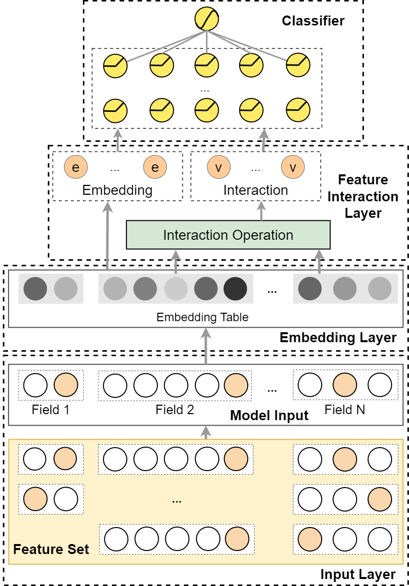
Figure 1. Overview of the general CTR framework.

In this paper, we propose a method, Optimizing Feature Set (OptFS), to address the problem of searching the optimal feature set. There are two main challenges for our OptFS. The first challenge is how to select the feature and its interaction jointly, given various feature interaction operations. As discussed above, an optimal feature set should exclude features that introduce useless interaction in models. We tackle this challenge by decomposing the selection of each feature interaction into the selection of two correlated features. Therefore, OptFS reduces the search space of feature interaction and trains the model end-to-end, given various feature interaction operations. The second challenge is the number of features in large-scale datasets. Notice that the possible number of features considered in our research could be $10^{6}$, which is incredibly larger than $100$ feature fields in previous works (Wang et al., 2022; Guo et al., 2022). To navigate in the large search space, we introduce a learnable gate for each feature and adopt the learning-by-continuation (Liu et al., 2020a; Savarese et al., 2020; Yuan et al., 2021) training scheme. We summarize our major contributions as follows:

• This paper first distinguishes the optimal feature set problem, which focuses on the feature level and considers the effectiveness of both feature and feature interaction, improving the model performance and computation efficiency.

• We propose a novel method named OptFS that optimizes the feature set. Developing an efficient learning-by-continuation training scheme, OptFS leverages feature interaction operations trained together with the prediction model in an end-to-end manner.

• Extensive experiments are conducted on three large-scale public datasets. The experimental results demonstrate the effectiveness and efficiency of the proposed method.

We organize the rest of the paper as follows. In Section 2, we formulate the CTR prediction and feature selection problem and propose a simple but effective method OptFS. Section 3 details the experiments. In Section 4, we briefly introduce related works. Finally, we conclude this paper in Section 5.

2. OptFS

In this section, we will first distinguish the feature set optimization problem in Section 2.1 and detail how OptFS conduct feature selection in Section 2.2. Then, we will illustrate how OptFS influences feature interaction selection in Section 2.3. Finally, we will illustrate the learning-by-continuation method in Section 2.4.

2.1. Problem Formulation

In this subsection, we provide a formulation of the feature set optimization problem. Usually, features that benefit the accurate prediction are considered useful in CTR models. In our setting, we represent all possible features as $\mathbf{X}=\{\mathbf{x}_{1},\mathbf{x}_{2},\cdots,\mathbf{x}_{m}\}$. $\mathbf{x}_{i}$ is a one-hot representation, which is very sparse and high-dimensional. As previously discussed, the feature set optimization problem aims to determine the useful features among all possible ones, which can be defined as finding an optimal feature set $\mathbf{X}^{\mathbf{g}}\subset\mathbf{X}$. This can be formulated as follows:

(1) $$\min_{\mathbf{W}}\mathcal{L}(\mathcal{D}|\mathbf{W}) ,\ \mathcal{D}=\{\mathbf{X}^{\mathbf{g}},\mathbf{Y}\},$$

$$s.t.\forall\mathbf{x}\in\mathbf{X}^{\mathbf{g}},\mathcal{L}(\mathbf{X}^{\mathbf{g}}) >\mathcal{L}(\mathbf{X}^{\mathbf{g}}-\{\mathbf{x}\}),$$

$$\forall\mathbf{x}\notin\mathbf{X}^{\mathbf{g}},\mathcal{L}(\mathbf{X}^{\mathbf{g}}) \geq\mathcal{L}(\mathbf{X}^{\mathbf{g}}+\{\mathbf{x}\}),$$

where $\mathcal{L}$ denotes the loss function, $\mathbf{W}$ denotes the model parameters, and $\mathbf{Y}$ denotes the corresponding labels.

2.2. Feature Selection

Each field $\mathbf{z}_{i}$ contains a proportion of all possible features, denoted as:

(2) $$\mathbf{z}_{i}=\{\mathbf{x}_{k_{i}}\},\ 1\leq k_{i}\leq m,$$

which indicates that the relationship between field and feature is a one-to-many mapping. In practice, the number of field $n$ is much smaller than that of feature $m$. For instance, online advertisement systems usually have $n\leq 100$ and $m\approx 10^{6}$. So the input of CTR models can be rewritten as follows from both feature and field perspectives:

(3) $$\mathbf{z}=[\mathbf{z}_{1},\mathbf{z}_{2},\cdots,\mathbf{z}_{n}]=[\mathbf{x}_{k_{1}},\mathbf{x}_{k_{2}},\cdots,\mathbf{x}_{k_{n}}],$$

where the second equal sign means that for input $\mathbf{z}$, the corresponding feature for field $\mathbf{z}_{i}$ is $\mathbf{x}_{k_{i}}$ as shown in Equation 2.

We usually employ embedding tables to convert $\mathbf{z}_{i}$s into low-dimensional and dense real-value vectors. This can be formulated as $\mathbf{e}_{i}=\mathbf{E}\times\mathbf{z}_{i}=\mathbf{E}\times\mathbf{x}_{k_{i}},1\leq i\leq n,1\leq k_{i}\leq m$, where $\mathbf{E}\in\mathbb{R}^{m\times D}$ is the embedding table, $m$ is the number of feature values and $D$ is the size of embedding. Then embeddings are stacked together as a embedding vector $\mathbf{e}=[\mathbf{e}_{1},\mathbf{e}_{2},\cdots,\mathbf{e}_{n}]$.

In our work, we propose feature-level selection. Instead of doing field-level selection, we formulate selection as assigning a binary gate $\mathbf{g}_{k_{i}}\in\{0,1\}$ for each feature embedding $\mathbf{e}_{k_{i}}$. After selection, the feature embeddings can be formulated as follows:

(4) $$\mathbf{e}_{k_{i}}^{\mathbf{g}}=\mathbf{g}_{k_{i}}\odot\mathbf{e}_{k_{i}}=\mathbf{g}_{k_{i}}\odot(\mathbf{E}\times\mathbf{x}_{k_{i}}).$$

When $\mathbf{g}_{k_{i}}=1$, feature $\mathbf{x}_{k_{i}}$ is in the optimal feature set $\mathbf{X}^{\mathbf{g}}$ and vice versa. Notice that previous work (Tibshirani, 1996; Guo et al., 2022; Wang et al., 2022) assigns field-level feature selection. This means that $\mathbf{g}_{k_{i}}\equiv\mathbf{g}_{i}\in\{0,1\}$ for each field $z_{i}$, indicating the keep or drop of all possible features $\{\mathbf{x}_{k_{i}}\}$ in corresponding field.

Then, these embeddings are stacked together as a feature-selected embedding vector $\mathbf{e}^{\mathbf{g}}=[\mathbf{e}_{k_{1}}^{\mathbf{g}},\mathbf{e}_{k_{2}}^{\mathbf{g}},\cdots,\mathbf{e}_{k_{n}}^{\mathbf{g}}]$. The final prediction can be formulated as follows:

(5) $$\hat{y}=\mathcal{F}(\mathbf{g}\odot\mathbf{E}\times\mathbf{x}|\mathbf{W})=\mathcal{F}(\mathbf{E}^{\mathbf{g}}\times\mathbf{x}|\mathbf{W}),$$

where $\mathbf{g}\in\{0,1\}^{m}$ refers to gating vectors indicating whether certain feature is selected or not, $\mathbf{E}^{\mathbf{g}}=\mathbf{g}\odot\mathbf{E}$ indicates the feature-selected embedding tables. The $\mathbf{E}^{\mathbf{g}}$ can also be viewed as the feature set $\mathbf{X}^{\mathbf{g}}$ after transformation from the embedding table, denoted as $\mathbf{E}^{\mathbf{g}}=\mathbf{E}\times\mathbf{X}^{\mathbf{g}}$.

2.3. Feature Interaction Selection

The feature interaction selection aims to select beneficial feature interaction for explicitly modelling (Lyu et al., 2022a; Liu et al., 2020b). The feature interaction layer will be performed based on $\mathbf{e}$ in mainstream CTR models. There are several types of feature interaction in previous study (Khawar et al., 2020), e.g. inner product (Guo et al., 2017). The interaction between two features $\mathbf{e}_{i}$ and $\mathbf{e}_{j}$ can be generally represented as:

(6) $$\mathbf{v}_{(i,j)}=\mathcal{O}(\mathbf{e}_{i},\mathbf{e}_{j}),$$

where $\mathcal{O}$, as the interaction operation, can vary from a single layer perceptron to cross layer(Wang et al., 2017). The feature interaction selection can be formulated as assigning $\mathbf{g}^{{}^{\prime}}_{(i,j)}$ for each feature interaction. All feature interactions can be aggregated together for final prediction:

(7) $$\hat{y}=\mathcal{H}((\mathbf{g}^{{}^{\prime}}\odot\mathbf{v})\oplus\mathcal{G}(\mathbf{e}^{\mathbf{g}}))=\mathcal{H}(\mathbf{v}^{\mathbf{g}^{{}^{\prime}}}\oplus\mathcal{G}(\mathbf{e}^{\mathbf{g}})),$$

where symbol $\oplus$ denotes the concatenation operation, $\mathcal{G}(\cdot)$ denotes the transformation function from embedding space to feature interaction space, such as MLP (Guo et al., 2017; Wang et al., 2017) or null function (Qu et al., 2016). $\mathcal{H}(\cdot)$ represents the prediction function. The combinations of $\mathcal{G}(\cdot)$, $\mathcal{O}(\cdot)$ and $\mathcal{H}(\cdot)$ in mainstream models are summarized in Table 1.

Table 1. Summary of $\mathcal{G}(\cdot)$, $\mathcal{O}(\cdot)$ and $\mathcal{H}(\cdot)$ in mainstream models

Model	$\mathcal{G}(\cdot)$	$\mathcal{O}(\cdot)$	$\mathcal{H}(\cdot)$
FM (Rendle, 2010)	null	inner product	null
DeepFM (Guo et al., 2017)	MLP	inner product	average
DCN (Wang et al., 2017)	MLP	cross network	average
IPNN (Qu et al., 2016)	null	inner product	MLP
OPNN (Qu et al., 2016)	null	outer product	MLP
PIN (Qu et al., 2019)	null	MLP	MLP

In reality, a direct way to explore all possible feature interaction is introducing a feature interaction matrix $\{\mathbf{g}^{{}^{\prime}}_{(k_{i},k_{j})}\}$ for 2nd-order feature interaction $\{\mathbf{x}_{k_{i}},\mathbf{x}_{k_{j}}\}$. But it is impossible as we would have $C_{m}^{2}\approx 10^{12}$ gate variables. To efficiently narrow down such a large space, previous works (Liu et al., 2020b; Khawar et al., 2020; Lyu et al., 2022a) restrict the search space to feature field interaction, reducing the number of variables to $C_{n}^{2}\approx 1000$. This can be formulated as $\mathbf{g}^{{}^{\prime}}_{(i,j)}\equiv\mathbf{g}^{{}^{\prime}}_{(k_{i},k_{j})}$. However, such relaxation may not be able to distinguish the difference between useful and useless feature interaction within the same field. As it has been proven that informative interaction between features tends to come from the informative lower-order ones (Xie et al., 2021), we decompose the feature interaction as follows:

(8) $$\mathbf{g}^{{}^{\prime}}_{(k_{i},k_{j})}=\mathbf{g}_{k_{i}}\times\mathbf{g}_{k_{j}},$$

which indicates that the feature interaction is only deemed useful when both features are useful. An illustration of the decomposition is shown in Figure 2. Hence, the final prediction can be written as:

(9) $$\hat{y}=\mathcal{H}((\mathbf{g}\times\mathbf{g}\odot\mathbf{v})\oplus\mathcal{G}(\mathbf{g}\odot\mathbf{e})),$$

which means that the gating vector $\mathbf{g}$ that selects features can also select the feature interaction given $\mathcal{O}(\cdot)$. Such a design can reduce the search space and obtain the optimal feature set in an end-to-end manner.

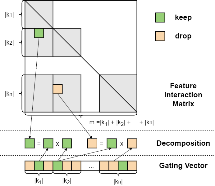
Figure 2. The Overview of OptFS.

2.4. Learning by Continuation

Even though the search space has been narrowed down from $C^{2}_{m}+m$ to $m$ in Section 2.3, we still need to determine whether to keep or drop each feature in the feature set. This can be formulated as a $\mathcal{l}_{0}$ normalization problem. However, binary gate vector $m$ is hard to compute valid gradient. Moreover, $\mathcal{l}_{0}$ optimization is known as a NP-hard problem (Natarajan, 1995). To efficiently train the entire model, we introduce a learning-by-continuation training scheme. Such a training scheme has proven to be an efficient method for approximating $\mathcal{l}_{0}$ normalization (Savarese et al., 2020), which correlates with our goal.

The learning-by-continuation training scheme consists of two parts: the searching stage that determines the gating vector $\mathbf{g}$ and the rewinding stage that determines the embedding table $\mathbf{e}$ and other parameters $\mathbf{W}$. We will introduce them separately in the following sections.

2.4.1. Searching

To efficiently optimize the feature set with feature-level granularity, we introduce a continual gate $\mathbf{g}_{c}\in\mathbb{R}^{m}$. During the searching stage, we introduce an exponentially-increased temperature value $\tau$ to approximate $L_{0}$ normalization. Specifically, the actual gate $\mathbf{g}$ is computed as:

(10) $$\mathbf{g}=\frac{\sigma(\mathbf{g}_{c}\times\tau)}{\sigma(\mathbf{g}_{c}^{(0)})},\ \tau=\gamma^{t/T}$$

where $\mathbf{g}_{c}^{(0)}$ is the initial value of the continual gate $\mathbf{g}_{c}$, $\sigma$ is the sigmoid function $\sigma(x)=\frac{1}{1+e^{-x}}$ applied element-wise, $t$ is the current training epoch number, $T$ is the total training epoch and $\gamma$ is the final value of $\tau$ after training for $T$ epochs. This would allow the continuous gating vector $\mathbf{g}_{c}$ to receive valid gradients in early stages yet increasingly approximate binary gate as the epoch number $t$ grows. An illustration of Equation 10 is shown in Figure 3(a).

The final prediction is calculated based on Equation 9. The cross-entropy loss (i.e. log-loss) is adopted for each sample:

(11) $$\text{CE}(y,\hat{y})=y\log(\hat{y})+(1-y)\log(1-\hat{y}),$$

where $y$ is the ground truth of user clicks. We summarize the final accuracy loss as follows:

(12) $$\mathcal{L}_{\text{CE}}(\mathcal{D}|\{\mathbf{E},\mathbf{W}\})=-\frac{1}{|\mathcal{D}|}\sum_{(\mathbf{x},y)\in\mathcal{D}}\text{CE}(y,\mathcal{F}(\mathbf{E}\times\mathbf{x}|\mathbf{W})),$$

where $\mathcal{D}$ is the training dataset and $\mathbf{W}$ is network parameters except the embedding table $\mathbf{E}$. Hence, the final training objective becomes:

(13) $$\min_{\mathbf{g}_{c},\mathbf{E},\mathbf{W}}\ \mathcal{L}_{\text{CE}}(\mathcal{D}|\{\mathbf{g}_{c}\odot\mathbf{E},\mathbf{W}\})+\lambda\lVert\mathbf{g}\rVert_{1},$$

where $\lambda$ is the regularization penalty, $\lVert\cdot\rVert_{1}$ indicates the $\mathcal{l}_{1}$ norm to encourage sparsity. Here we restate $\mathcal{l}_{0}$ norm to $\mathcal{l}_{1}$ norm given the fact that $\lVert\mathbf{g}\rVert_{0}=\lVert\mathbf{g}\rVert_{1}$ for binary $\mathbf{g}$.

After training $T$ epochs, the final gating vector $\mathbf{g}$ is calculated through a unit-step function as follows:

(14) $$\mathbf{g}=\begin{cases}0,\quad&\mathbf{g}_{c}\leq 0\\ 1,\quad&\text{otherwise}\end{cases}.$$

Such a unit step function is also visualized in Figure 3(b).

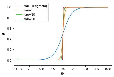
(a) Searching Stage

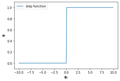
(b) Re-training Stage

Figure 3. Visualization of gating vector $g$ during searching and retraining stages.

2.4.2. Retraining

In the searching stage, all possible features are fed into the model to explore the optimal feature set $\mathbf{X}^{\mathbf{g}}$. Thus, the useless features might hurt the model’s performance. To address this problem, we need to retrain the model after obtaining the optimal feature set $\mathbf{X}^{\mathbf{g}}$.

After determining the gating vector $\mathbf{g}$, we retrain the model parameters $\mathbf{E}$ and $\mathbf{W}$ as the corresponding values at $T_{c}$ epoch, which is carefully tuned in our setting. This is because most CTR models early stopped in several epochs, making them more sensitive towards initialization and prone to overfitting (Zhang et al., 2022). The final parameters $\mathbf{E}$ and $\mathbf{W}$ are trained as follows:

(15) $$\min_{\mathbf{E},\mathbf{W}}\ \mathcal{L}_{\text{CE}}(\mathcal{D}|\{\mathbf{g}\odot\mathbf{E},\mathbf{W}\}).$$

The overall process of our model is summarized in Algorithm 1.

Algorithm 1 The OptFS Algorithm

1:training dataset $\mathcal{D}$, initialization epoch $T_{c}$, total epoch $T$

2:gating vector $\mathbf{g}$, model parameters {$\mathbf{E}$, $\mathbf{W}$}

3:## Searching ##

4:t=0

5:while t ¡ T do

6:     t = t + 1

7:     while $\mathcal{D}$ is not fully iterated do

8:         Sample a mini-batch from the training dataset

9:         $\{\mathbf{E}_{t},\mathbf{W}_{t}\}$, $\mathbf{g}$ = Searching($\mathcal{D}$) $\triangleright$ Equation 13

10:     end while

11:     if $t==T_{c}$ then

12:         $\{\hat{\mathbf{E}},\hat{\mathbf{W}}\}\Leftarrow\{\mathbf{E}_{t},\mathbf{W}_{t}\}$

13:     end if

14:end while

15:$\mathbf{g}$ = Discretization($\{\mathbf{g}_{c}\}$) $\triangleright$ Equation 14

16:## Retraining##

17:Retrain $\{\mathbf{E},\mathbf{W}\}$ given $\mathbf{g}$ with $\{\hat{\mathbf{E}},\hat{\mathbf{W}}\}$ as initialization $\triangleright$ Equation 15

3. experiment

In this section, to comprehensively evaluate our proposed method, we design experiments to answer the following research questions:

• RQ1: Could OptFS achieve superior performance compared with mainstream feature (interaction) selection methods?

• RQ2: How does the end-to-end training scheme influence the model performance?

• RQ3: How does the re-training stage influence the performance?

• RQ4: How efficient is OptFS compared to other feature (interaction) selection methods?

• RQ5: Does OptFS select the optimal features?

Table 2. Performance Comparison Between OptFS and Feature Selection Methods.

	Method	FM			DeepFM			DCN			IPNN
		AUC$\uparrow$	Logloss$\downarrow$	Ratio$\downarrow$	AUC$\uparrow$	Logloss$\downarrow$	Ratio$\downarrow$	AUC$\uparrow$	Logloss$\downarrow$	Ratio$\downarrow$	AUC$\uparrow$	Logloss$\downarrow$	Ratio$\downarrow$
Criteo	Backbone	0.8055	0.4457	1.0000	0.8089	0.4426	1.0000	0.8107	0.4410	1.0000	0.8110	0.4407	1.0000
	LPFS	0.7888	0.4604	0.0157	0.7915	0.4579	0.2415	0.7802	0.4743	0.1177	0.7789	0.4705	0.3457
	AutoField	0.7932	0.4567	0.0008	0.8072	0.4439	0.3811	0.8113	0.4402	0.5900	0.8115	0.4401	0.9997
	AdaFS	0.7897	0.4597	1.0000	0.8005	0.4501	1.0000	0.8053	0.4472	1.0000	0.8065	0.4448	1.0000
	OptFS	0.8060	0.4454	0.1387	$\textbf{0.8100}^{*}$	$\textbf{0.4415}^{*}$	0.0422	0.8111	0.4405	0.0802	0.8116	0.4401	0.0719
Avazu	Backbone	0.7838	0.3788	1.0000	0.7901	0.3757	1.0000	0.7899	0.3755	1.0000	0.7913	0.3744	1.0000
	LPFS	0.7408	0.4029	0.7735	0.7635	0.3942	0.9975	0.7675	0.3889	0.9967	0.7685	0.3883	0.9967
	AutoField	0.7680	0.3862	0.0061	0.7870	0.3773	1.0000	0.7836	0.3782	0.9992	0.7865	0.3770	0.9992
	AdaFS	0.7596	0.3913	1.0000	0.7797	0.3837	1.0000	0.7693	0.3954	1.0000	0.7818	0.3833	1.0000
	OptFS	0.7839	0.3784	0.8096	$\textbf{0.7946}^{*}$	$\textbf{0.3712}^{*}$	0.8686	$\textbf{0.7932}^{*}$	$\textbf{0.3718}^{*}$	0.8665	$\textbf{0.7950}^{*}$	$\textbf{0.3709}^{*}$	0.9118
KDD12	Backbone	0.7783	0.1566	1.0000	0.7967	0.1531	1.0000	0.7974	0.1531	1.0000	0.7966	0.1532	1.0000
	LPFS	0.7725	0.1578	1.0000	0.7964	0.1532	1.0000	0.7970	0.1530	1.0000	0.7967	0.1532	1.0000
	AutoField	0.7411	0.1634	0.0040	0.7919	0.1542	0.9962	0.7943	0.1536	0.8249	0.7926	0.1541	0.8761
	AdaFS	0.7418	0.1644	1.0000	0.7917	0.1543	1.0000	0.7939	0.1538	1.0000	0.7936	0.1539	1.0000
	OptFS	$\textbf{0.7811}^{*}$	$\textbf{0.1560}^{*}$	0.5773	$\textbf{0.7988}^{*}$	$\textbf{0.1527}^{*}$	0.9046	$\textbf{0.7981}^{*}$	0.1530	0.8942	0.7975	0.1530	0.8729

• Here $*$ denotes statistically significant improvement (measured by a two-sided t-test with p-value $<0.05$) over the best baseline. Bold font indicates the best-performed method.

3.1. Experiment Setup

3.1.1. Datasets

We conduct our experiments on three public real-world datasets. We describe all datasets and the pre-processing steps below.

Criteo dataset consists of ad click data over a week. It consists of 26 categorical feature fields and 13 numerical feature fields. Following the best practice (Zhu et al., 2021), we discretize each numeric value $x$ to $\lfloor\log^{2}(x)\rfloor$, if $x>2$; $x=1$ otherwise. We replace infrequent categorical features with a default ”OOV” (i.e. out-of-vocabulary) token, with min_count=10.

Avazu dataset contains 10 days of click logs. It has 24 fields with categorical features. Following the best practice (Zhu et al., 2021), we remove the instance_id field and transform the timestamp field into three new fields: hour, weekday and is_weekend. We replace infrequent categorical features with the ”OOV” token, with min_count=10.

KDD12 dataset contains training instances derived from search session logs. It has 11 categorical fields, and the click field is the number of times the user clicks the ad. We replace infrequent features with an ”OOV” token, with min_count=10.

3.1.2. Metrics

Following the previous works (Rendle, 2010; Guo et al., 2017), we use the common evaluation metrics for CTR prediction: AUC (Area Under ROC) and Log loss (cross-entropy). Note that $\mathbf{0.1\%}$ improvement in AUC is considered significant (Qu et al., 2016; Guo et al., 2017). To measure the size of the feature set, we normalize it based on the following equation:

(16) $$\text{Ratio}=\text{\#Remaining Features}/m.$$

3.1.3. Baseline Methods and Backbone Models

We compare the proposed method OptFS with the following feature selection methods: (i) AutoField (Wang et al., 2022): This baseline utilizes neural architecture search techniques (Liu et al., 2019) to select the informative features on a field level; (ii) LPFS (Guo et al., 2022): This baseline designs a customized, smoothed-$\mathcal{l}_{0}$-liked function to select informative fields on a field level; (iii) AdaFS (Lin et al., 2022): This baseline that selects the most relevant features for each sample via a novel controller network. We apply the above baselines over the following mainstream backbone models: FM (Rendle, 2010), DeepFM (Guo et al., 2017), DCN (Wang et al., 2017) and IPNN (Qu et al., 2016).

We also compare the proposed method OptFS with a feature interaction selection method: AutoFIS (Liu et al., 2020b). This baseline utilizes GRDA optimizer to abandon unimportant feature interaction in a field-level manner. We apply AutoFIS over the following backbone models: FM (Rendle, 2010), DeepFM (Guo et al., 2017). We only compare with AutoFIS on FM and DeepFM backbone models because the original paper only provides the optimal hyper-parameter settings and releases source code under these settings.

3.1.4. Implementation Details

In this section, we provide the implementation details. For OptFS, (i) General hyper-params: We set the embedding dimension as 16 and batch size as 4096. For the MLP layer, we use three fully-connected layers of size [1024, 512, 256]. Following previous work (Qu et al., 2016), Adam optimizer, Batch Normalization (Ioffe and Szegedy, 2015) and Xavier initialization (Glorot and Bengio, 2010) are adopted. We select the optimal learning ratio from {1e-3, 3e-4, 1e-4, 3e-5, 1e-5} and $l_{2}$ regularization from {1e-3, 3e-4, 1e-4, 3e-5, 1e-5, 3e-6, 1e-6}. (ii) OptFS hyper-params: we select the optimal regularization penalty $\lambda$ from {1e-8, 5e-9, 2e-9, 1e-9}, training epoch $T$ from {5, 10, 15}, final value $\gamma$ from {2e+2, 5e+2, 1e+3, 2e+3, 5e+3, 1e+4}. During the re-training phase, we reuse the optimal learning ratio and $l_{2}$ regularization and choose the rewinding epoch $T_{c}$ from $\{1,2,\cdots,T-1\}$. For AutoField and AdaFS, we select the optimal hyper-parameter from the same hyper-parameter domain of OptFS, given the original paper does not provide the hyper-parameter settings. For LPFS and AutoFIS, we reuse the optimal hyper-parameter mentioned in original papers.

Our implementation is based on a public Pytorch library for CTR prediction. For other baseline methods, we reuse the official implementation for the AutoFIS (Liu et al., 2020b) method. Due to the lack of available implementations for the LPFS (Guo et al., 2022), AdaFS(Lin et al., 2022) and AutoField(Wang et al., 2022) methods, we re-implement them based on the details provided by the authors and open-source them to benefit future researchers.

3.2. Overall Performance(RQ1)

In this section, we conduct two studies to separately compare feature selection methods and feature interaction selection methods in Section 3.2.1 and 3.2.2. Notes that both these methods can be viewed as a solution to the feature set optimization problem.

3.2.1. Feature Selection

The overall performance of our OptFS and other feature selection baseline methods on four different backbone models using three benchmark datasets are reported in Table 2. We summarize our observation below.

Firstly, our OptFS is effective and efficient compared with other baseline methods. OptFS can achieve higher AUC with a lower feature ratio. However, the benefit brought by OptFS differs on various datasets. On Criteo, OptFS tends to reduce the size of the feature set. OptFS can reduce 86% to 96% features with improvement not considered significant statistically. On the Avazu and KDD12 datasets, the benefit tends to be both performance boosting and feature reduction. OptFS can significantly increase the AUC by 0.01% to 0.45% compared with the backbone model while using roughly 10% of the features. Note that the improved performance is because OptFS considers feature interaction’s influence during selection. Meanwhile, other feature selection baselines tend to bring performance degradation. This is likely because they adopt the feature field selection. Such a design will inevitably drop useful features or keep useless ones.

Secondly, different datasets behave differently regarding the redundancy of features. For example, on the Criteo dataset, all methods produce low feature ratios, indicating that this dataset contains many redundant features. On the other hand, on the Avazu and KDD12 datasets, all methods produce high feature ratios, suggesting that these two datasets have lower redundancy. OptFS can better balance the trade-off between model performance and efficiency compared with other baselines in all datasets.

Finally, field-level feature selection methods achieve different results on various backbone models. Compared to other deep models, FM solely relies on the explicit interaction, i.e. inner product. If one field $\mathbf{z}_{i}$ is zeroed out during the process, all its related interactions will be zero. The other fields are also lured into zero, as their interaction with field $\mathbf{z}_{i}$ does not bring any information into the final prediction. Therefore, it can be observed that LPFS has a low feature ratio on Criteo and high feature ratios on Avazu and KDD12 datasets. On the other hand, AutoField generates low feature ratios ($\sim$0%) on all three datasets. These observations further highlight the necessity of introducing feature-level granularity into the feature set optimization problem as OptFS does.

3.2.2. Feature Interaction Selection

Table 3. Performance Comparison Between OptFS and Feature Interaction Selection Method.

	Model	Method	Metrics
			AUC$\uparrow$	Logloss$\downarrow$	Ratio$\downarrow$
Criteo	FM	Backbone	0.8055	0.4457	1.0000
		AutoFIS	0.8063	0.4449	1.0000
		OptFS	0.8060	0.4454	0.1387
	DeepFM	Backbone	0.8089	0.4426	1.0000
		AutoFIS	0.8097	0.4418	1.0000
		OptFS	0.8100	0.4415	0.0422
Avazu	FM	Backbone	0.7838	0.3788	1.0000
		AutoFIS	0.7843	0.3785	1.0000
		OptFS	0.7839	0.3784	0.8096
	DeepFM	Backbone	0.7901	0.3757	1.0000
		AutoFIS	0.7928	0.3721	1.0000
		OptFS	$\textbf{0.7946}^{*}$	$\textbf{0.3712}^{*}$	0.8686

• Here $*$ denotes statistically significant improvement (measured by a two-sided t-test with p-value $<0.05$) over the best baseline. Bold font indicates the best-performed method.

In this subsection, we aim to study the influence of the OptFS method on feature interaction selection. The overall performance of our OptFS and AutoFIS on DeepFM and FM backbone models are reported in Table 3. We summarize our observation below.

Firstly, compared with backbone models that do not perform any feature interaction selection, AutoFIS and OptFS achieve higher performance. Such an observation points out the existence of useless feature interaction on both datasets.

Secondly, the performance of OptFS and AutoFIS differs on different models. With fewer features in the feature set, OptFS achieves nearly the same performance as AutoFIS on FM while performing significantly better on DeepFM. This is because OptFS focuses on feature-level interactions, which are more fine-grained than the field-level interactions adopted by AutoFIS.

Finally, it is also worth mentioning that OptFS can reduce $13$% to $96$% of features while AutoFIS is conducted on all possible features without any reduction.

3.3. Transferability Study(RQ2)

In this subsection, we investigate the transferability of OptFS’s result. The experimental settings are listed as follows. First, we search the gating vector $\mathbf{g}$ from one model, which we named the source. Then, we re-train another backbone model given the obtained gating vector, which we call the target. We study the transferability between DeepFM, DCN and IPNN backbone models over both Criteo and Avazu datasets. Based on the results shown in Table 4, we can easily observe that all transformation leads to performance degradation. Such degradation is even considered significant over the Avazu dataset. Therefore, feature interaction operations require different feature sets to achieve high performance. We can conclude that the selection of the feature set needs to incorporate the interaction operation, which further highlights the importance of selecting both features and their interactions in a unified, end-to-end trainable way.

Table 4. Transferability Analysis on Criteo and Avazu.

	Target	Source	Metrics
			AUC$\uparrow$	Logloss$\downarrow$	Ratio$\downarrow$
Criteo	DeepFM	DeepFM	0.8100	0.4415	0.0422
		DCN	0.8097	0.4419	0.0802
		IPNN	0.8097	0.4418	0.0719
	DCN	DCN	0.8111	0.4405	0.0802
		DeepFM	0.8106	0.4410	0.0422
		IPNN	0.8107	0.4410	0.0719
	IPNN	IPNN	0.8116	0.4401	0.0719
		DCN	0.8113	0.4404	0.0802
		DeepFM	0.8114	0.4403	0.0422
Avazu	DeepFM	DeepFM	$\textbf{0.7946}^{*}$	$\textbf{0.3712}^{*}$	0.8686
		DCN	0.7873	0.3754	0.8665
		IPNN	0.7872	0.3755	0.9118
	DCN	DCN	$\textbf{0.7932}^{*}$	$\textbf{0.3718}^{*}$	0.8665
		DeepFM	0.7879	0.3784	0.8686
		IPNN	0.7860	0.3762	0.9118
	IPNN	IPNN	$\textbf{0.7950}^{*}$	$\textbf{0.3709}^{*}$	0.9118
		DCN	0.7907	0.3747	0.8665
		DeepFM	0.7908	0.3748	0.8686

• Here $*$ denotes statistically significant improvement (measured by a two-sided t-test with p-value $<0.05$) over the best baseline. Bold font indicates the best-performed method.

3.4. Ablation Study(RQ3)

In this subsection, we conduct the ablation study over the influence of the re-training stage, which is detailedly illustrated in Section 2.4.2. In Section 2.4.2, we propose a customized initialization method, namely c.i., during the re-training stage. Here we compare it with the other three methods of obtaining model parameters: (i) w.o., which is the abbreviation for without re-training, directly inherit the model parameters from the searching stage; (ii) r.i. randomly initialize the model parameters; (iii) l.t.h., which stands for lottery ticket hypothesis, is a common method for re-training sparse network (Frankle and Carbin, 2019). Specifically, it initializes the model parameters with the same seed from the searching stage. The experiment is conducted over three backbone models, DeepFM, DCN and IPNN, over Criteo and Avazu benchmarks. We can make the following observations based on the result shown in Table 5.

Table 5. Ablation Study Regarding the Re-training Stage.

	Model	Metrics	Methods
			w.o.	r.i.	l.t.h.	c.i.
Criteo	DeepFM	AUC$\uparrow$	0.8012	0.8100	0.8100	0.8100
		Logloss$\downarrow$	0.4686	0.4416	0.4415	0.4415
	DCN	AUC$\uparrow$	0.8077	0.8109	0.8108	0.8111
		Logloss$\downarrow$	0.4522	0.4407	0.4408	0.4405
	IPNN	AUC$\uparrow$	0.7757	0.8113	0.8114	0.8116
		Logloss$\downarrow$	0.4998	0.4404	0.4403	0.4401
Avazu	DeepFM	AUC$\uparrow$	0.6972	0.7873	0.7883	$\textbf{0.7946}^{*}$
		Logloss$\downarrow$	0.5017	0.3754	0.3790	$\textbf{0.3712}^{*}$
	DCN	AUC$\uparrow$	0.7122	0.7870	0.7858	$\textbf{0.7932}^{*}$
		Logloss$\downarrow$	0.4736	0.3801	0.3764	$\textbf{0.3718}^{*}$
	IPNN	AUC$\uparrow$	0.7560	0.7912	0.7910	$\textbf{0.7950}^{*}$
		Logloss$\downarrow$	0.4411	0.3745	0.3745	$\textbf{0.3709}^{*}$

• Here $*$ denotes statistically significant improvement (measured by a two-sided t-test with p-value $<0.05$) over the best baseline. Bold font indicates the best-performed method.

• Here w.o. stands for without re-training, r.i. stands for re-training with random initialization, l.t.h. stands for initialization using lottery ticket hypothesis (Frankle and Carbin, 2019), c.i. stands for re-training with customized initialization, as previously discussed in Section 2.4.

Firstly, we can easily observe that re-training can improve performance regardless of its setting. Without re-training, the neural network will inherit the sub-optimal model parameters from the searching stage, which is influenced by the non-binary element in the gating vector. Re-training improves the model performance under the constraint of the gating vector.

Secondly, c.i. constantly outperforms the other two re-training methods. Such performance gaps are considered significant on all three backbone models over the Avazu dataset. This is likely because, on the Avazu dataset, the backbone models are usually trained for only one epoch before they get early-stopped for over-fitting. Hence, it further increases the importance of initialization during the re-training stage. This observation validates the necessity of introducing customized initialization in CTR prediction.

3.5. Efficiency Analysis(RQ4)

In addition to model performance, efficiency is vital when deploying the CTR prediction model in reality. In this section, we investigate the time and space complexity of OptFS.

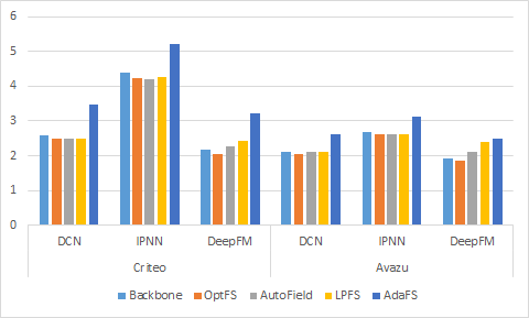
Figure 4. Inference Time of Different Models on Criteo and Avazu Dataset. The Y-axis represents the influence time, measured by ms

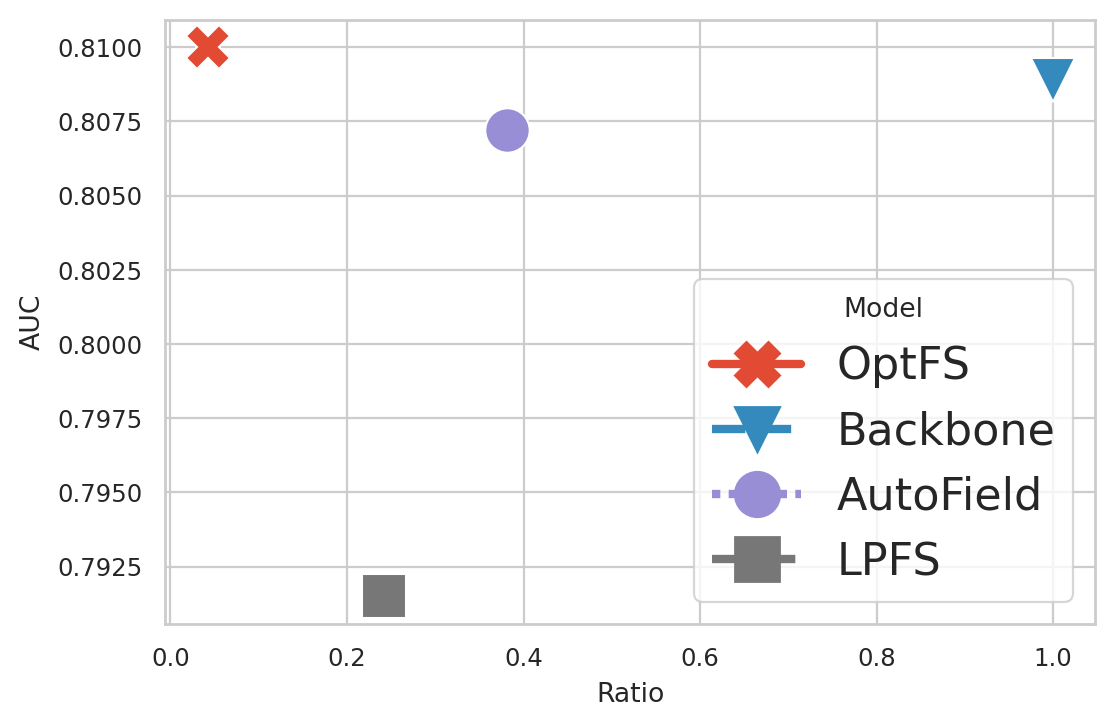
(a) DeepFM

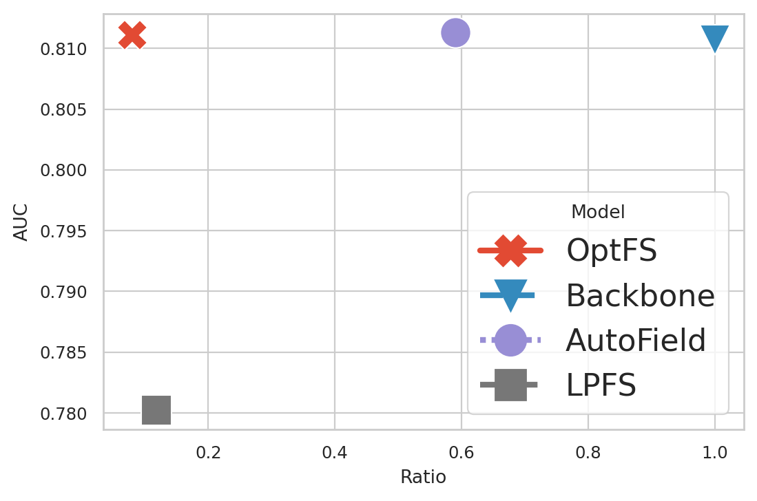
(b) DCN

Figure 5. Visualization of efficiency-effectiveness trade-off on Criteo datasets. The closer to the top-left the better.

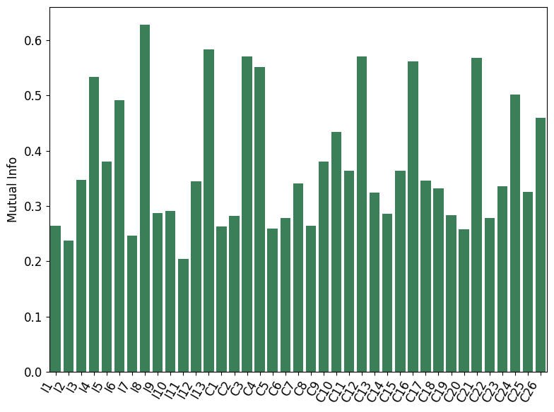
(a) Mutual Info

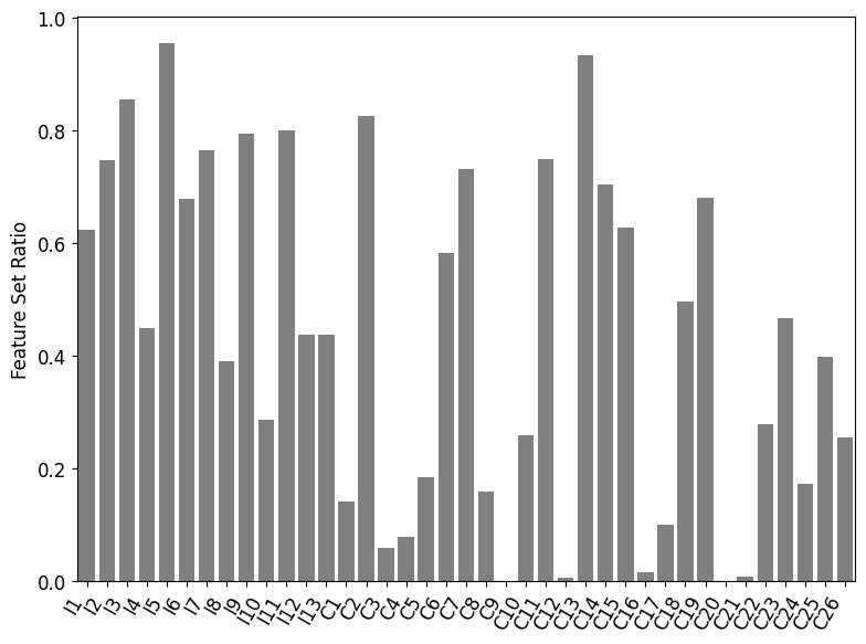
(b) DeepFM

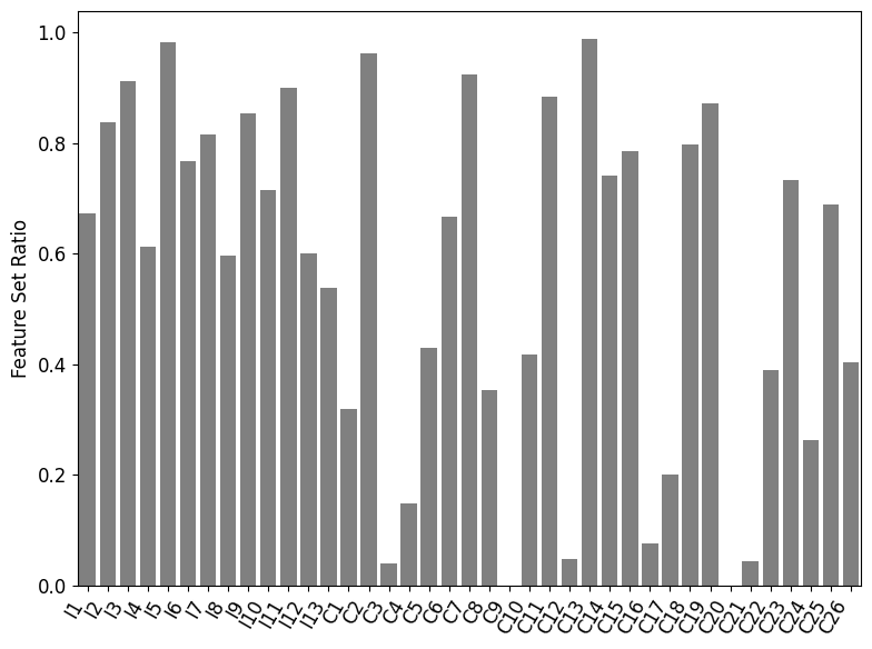
(c) DCN

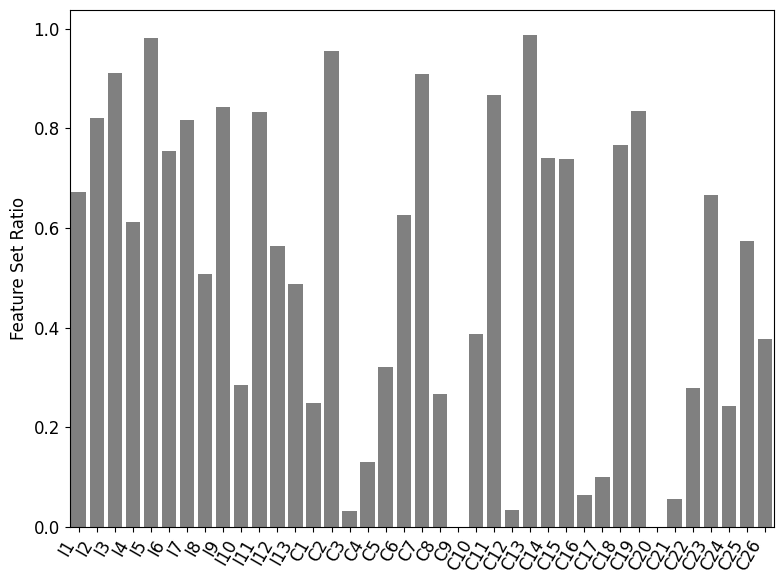
(d) IPNN

Figure 6. A Case Study of OptFS output on Criteo. In all subfigures, the X-axis indicates the field identifiers. Subfigure (a) plots the mutual information scores, while subfigures (b), (c) and (d) plot the feature set ratio of OptFS on DeepFM, DCN and IPNN.

3.5.1. Time Complexity

The inference time is crucial when deploying the model into online web systems. We define inference time as the time for inferencing one batch. The result is obtained by averaging the inference time over all batches on the validation set.

As shown in Figure 4, OptFS achieves the least inference time. This is because the feature set obtained by OptFS usually has the least features. Meanwhile, AdaFS requires the longest inference time, even longer than the backbone model. This is because it needs to determine whether keep or drop each feature dynamically during run-time.

3.5.2. Space Complexity

We plot the Feature Ratio-AUC curve of the DeepFM, DCN and IPNN model on the Criteo datasets in Figure 5, which reflects the relationship between the space complexity of the feature set and model performance. Notes that LPFS, AutoField and OptFS are methods that primarily aim to improve model performance. These methods have no guarantee over the final feature ratios. Hence we only plot one point for each method in the figure.

From Figure 5 we can make the following observations: (i) OptFS outperforms all other baselines with the highest AUC score and the least number of features. (ii) The model performance of AutoField is comparable with OptFS and Backbone. However, given it only selects the feature set on field-level, its feature ratio tends to be higher than OptFS. (iii) The performance of LPFS is much lower than other methods.

3.6. Case Study(RQ5)

This subsection uses a case study to investigate the optimal feature set obtained from OptFS. In Figure 6, we plot the mutual information with the feature ratio on each field. For field $\mathbf{z}_{i}=\{\mathbf{x}_{k_{i}}\}$ and ground truth labels $\mathbf{y}$ ($y\in\mathbf{y}$), the mutual information between them is defined as:

(17) $$\mathbf{MI}(\mathbf{x}_{k_{i}},\mathbf{y})=-\sum\mathbf{P}(y)\log\mathbf{P}(y)+\sum\mathbf{P}(\mathbf{x}_{k_{i}},y)\log\mathbf{P}(y|\mathbf{x}_{k_{i}}),$$

where the first term is the marginal entropy and the second term is the conditional entropy of ground truth labels $\mathbf{y}$ given field $\mathbf{z}_{i}=\{\mathbf{x}_{k_{i}}\}$. Note that fields with high mutual information scores are more informative (hence more important) to the prediction.

As a case study, we investigate the feature ratio for each field, shown in Figure 6. We select the result from DeepFM, DCN and IPNN on the Criteo dataset. Figure 6(a) shows the mutual information scores of each field, which represents how informative each field is in predicting the label. Figure 6(b), 6(c) and 6(d) shows the feature ratio given each fields. As can be seen, fields with higher mutual information scores are likely to keep more features in the feature set, which indicates that OptFS obtains the optimal feature set from the field perspective.

4. related work

In this section, we review the related work. Optimizing feature set is related two topics, feature selection and feature interaction selection. The training scheme of proposed OptFS is related to learning by continuation. Thus we summarize the related work in following two subsection.

4.1. Feature and Feature Interaction Selection

Feature selection is a key component for prediction task (Donà and Gallinari, 2021). Several methods have been proposed (Tibshirani, 1996; Liu et al., 2021; Wang et al., 2022; Guo et al., 2022; Lin et al., 2022) to conduct feature selection for CTR models. Traditional methods (Tibshirani, 1996; Liu et al., 2021) exploit the statistical metrics of different feature fields and conduct feature field selection. Inspired by neural architecture search (NAS) (Liu et al., 2019; Luo et al., 2018) and smoothed-$\mathcal{l}_{0}$ optimization respectively, AutoField (Wang et al., 2022) and LPFS (Guo et al., 2022) determine the selection of feature fields automatically. AdaFS (Lin et al., 2022) proposes a novel controller network to decide feature fields for each sample, which fits the dynamic recommendation. Feature interaction selection is often employed to enhance the prediction. Some methods (Liu et al., 2020b; Khawar et al., 2020) model the problem as NAS to exploit the field-level interaction space. OptInter (Lyu et al., 2022a) investigates the way to do feature interaction. AutoCross (Luo et al., 2019) targets on tabular data and iterative finds feature interaction based on locally optimized feature set. We first highlight the feature set optimization problem in CTR prediction, and OptFS is different from previous methods by solving both problems in a unified manner.

4.2. Learning by Continuation

Continuation methods are commonly used to approximate intractable optimization problems by gradually increasing the difficulty of the underlying objective. By adopting gradual relaxations to binary problems, gumbel-softmax (Jang et al., 2017) is used to back-propagate errors during the architecture search  (Wu et al., 2019) and spatial feature sparsification (Xie et al., 2020). Other methods (Savarese et al., 2020; Liu et al., 2020a; Yuan et al., 2021) introduce continuous sparsification framework to speed up neural network pruning and ticket search. OptFS adopts the learning-by-continuation scheme to effectively explore the huge feature-level search space.

5. conclusion

This paper first distinguishes the feature set optimization problem. Such a problem unifies two mutually influencing questions: the selection of features and feature interactions. To our knowledge, no previous work considers these two questions uniformly. Besides, we also upgrade the granularity of the problem from field-level to feature-level. To solve such the feature set optimization problem efficiently, we propose a novel method named OptFS, which assigns a gating value to each feature for its usefulness and adopt a learning-by-continuation approach for efficient optimization. Extensive experiments on three large-scale datasets demonstrate the superiority of OptFS in model performance and feature reduction. Several ablation studies also illustrate the necessity of our design. Moreover, we also interpret the obtained result on feature fields and their interactions, highlighting that our method properly solves the feature set optimization problem.

References

- (1)
- Bengio et al. (2013) Yoshua Bengio, Aaron C. Courville, and Pascal Vincent. 2013. Representation Learning: A Review and New Perspectives. IEEE Trans. Pattern Anal. Mach. Intell. 35, 8 (2013), 1798–1828. https://doi.org/10.1109/TPAMI.2013.50
- Chapelle et al. (2015) Olivier Chapelle, Eren Manavoglu, and Romer Rosales. 2015. Simple and Scalable Response Prediction for Display Advertising. ACM Trans. Intell. Syst. Technol. 5, 4 (dec 2015), 61.
- Donà and Gallinari (2021) Jérémie Donà and Patrick Gallinari. 2021. Differentiable Feature Selection, A Reparameterization Approach. In Machine Learning and Knowledge Discovery in Databases. Research Track - European Conference, ECML PKDD 2021 (Lecture Notes in Computer Science, Vol. 12977). Springer, Bilbao, Spain, 414–429. https://doi.org/10.1007/978-3-030-86523-8_25
- Frankle and Carbin (2019) Jonathan Frankle and Michael Carbin. 2019. The Lottery Ticket Hypothesis: Finding Sparse, Trainable Neural Networks. In 7th International Conference on Learning Representations, ICLR 2019. OpenReview.net, New Orleans, LA, USA.
- Glorot and Bengio (2010) Xavier Glorot and Yoshua Bengio. 2010. Understanding the difficulty of training deep feedforward neural networks. In 13th International Conference on Artificial Intelligence and Statistics, AISTATS 2010 (JMLR Proceedings, Vol. 9). JMLR.org, Italy, 249–256.
- Guo et al. (2021) Huifeng Guo, Wei Guo, Yong Gao, Ruiming Tang, Xiuqiang He, and Wenzhi Liu. 2021. ScaleFreeCTR: MixCache-based Distributed Training System for CTR Models with Huge Embedding Table. In SIGIR ’21: The 44th International ACM SIGIR Conference on Research and Development in Information Retrieval. ACM, Virtual Event, Canada, 1269–1278. https://doi.org/10.1145/3404835.3462976
- Guo et al. (2017) Huifeng Guo, Ruiming Tang, Yunming Ye, Zhenguo Li, and Xiuqiang He. 2017. DeepFM: A Factorization-Machine based Neural Network for CTR Prediction. In 26th International Joint Conference on Artificial Intelligence, IJCAI 2017. ijcai.org, Melbourne, Australia, 1725–1731.
- Guo et al. (2022) Yi Guo, Zhaocheng Liu, Jianchao Tan, Chao Liao, Daqing Chang, Qiang Liu, Sen Yang, Ji Liu, Dongying Kong, Zhi Chen, and Chengru Song. 2022. LPFS: Learnable Polarizing Feature Selection for Click-Through Rate Prediction. CoRR abs/2206.00267 (2022). https://doi.org/10.48550/arXiv.2206.00267 arXiv:2206.00267
- Hastie et al. (2009) Trevor Hastie, Robert Tibshirani, and Jerome H. Friedman. 2009. The Elements of Statistical Learning: Data Mining, Inference, and Prediction, 2nd Edition. Springer, Berlin, Germany. https://doi.org/10.1007/978-0-387-84858-7
- Ioffe and Szegedy (2015) Sergey Ioffe and Christian Szegedy. 2015. Batch Normalization: Accelerating Deep Network Training by Reducing Internal Covariate Shift. In 32nd International Conference on Machine Learning, ICML 2015 (JMLR Workshop and Conference Proceedings, Vol. 37). JMLR.org, France, 448–456.
- Jang et al. (2017) Eric Jang, Shixiang Gu, and Ben Poole. 2017. Categorical Reparameterization with Gumbel-Softmax. In 5th International Conference on Learning Representations, ICLR 2017. OpenReview.net, Toulon, France.
- Khawar et al. (2020) Farhan Khawar, Xu Hang, Ruiming Tang, Bin Liu, Zhenguo Li, and Xiuqiang He. 2020. AutoFeature: Searching for Feature Interactions and Their Architectures for Click-through Rate Prediction. In CIKM ’20: The 29th ACM International Conference on Information and Knowledge Management. ACM, Virtual Event, Ireland, 625–634. https://doi.org/10.1145/3340531.3411912
- Lin et al. (2022) Weilin Lin, Xiangyu Zhao, Yejing Wang, Tong Xu, and Xian Wu. 2022. AdaFS: Adaptive Feature Selection in Deep Recommender System. In KDD ’22: The 28th ACM SIGKDD Conference on Knowledge Discovery and Data Mining. ACM, Washington, DC, USA, 3309–3317. https://doi.org/10.1145/3534678.3539204
- Liu et al. (2020b) Bin Liu, Chenxu Zhu, Guilin Li, Weinan Zhang, Jincai Lai, Ruiming Tang, Xiuqiang He, Zhenguo Li, and Yong Yu. 2020b. AutoFIS: Automatic Feature Interaction Selection in Factorization Models for Click-Through Rate Prediction. In KDD ’20: The 26th ACM SIGKDD Conference on Knowledge Discovery and Data Mining. ACM, Virtual Event, CA, USA, 2636–2645. https://doi.org/10.1145/3394486.3403314
- Liu et al. (2019) Hanxiao Liu, Karen Simonyan, and Yiming Yang. 2019. DARTS: Differentiable Architecture Search. In 7th International Conference on Learning Representations, ICLR 2019. OpenReview.net, USA.
- Liu et al. (2020a) Junjie Liu, Zhe Xu, Runbin Shi, Ray C. C. Cheung, and Hayden Kwok-Hay So. 2020a. Dynamic Sparse Training: Find Efficient Sparse Network From Scratch With Trainable Masked Layers. In 8th International Conference on Learning Representations, ICLR 2020. OpenReview.net, Addis Ababa, Ethiopia.
- Liu et al. (2021) Qiang Liu, Zhaocheng Liu, Haoli Zhang, Yuntian Chen, and Jun Zhu. 2021. Mining Cross Features for Financial Credit Risk Assessment. In CIKM ’21: The 30th ACM International Conference on Information and Knowledge Management. ACM, Virtual Event, Queensland, Australia, 1069–1078. https://doi.org/10.1145/3459637.3482371
- Luo et al. (2018) Renqian Luo, Fei Tian, Tao Qin, Enhong Chen, and Tie-Yan Liu. 2018. Neural Architecture Optimization. In 31st Annual Conference on Neural Information Processing Systems 2018, NeurIPS 2018. Curran Associates, Montréal, Canada, 7827–7838.
- Luo et al. (2019) Yuanfei Luo, Mengshuo Wang, Hao Zhou, Quanming Yao, Wei-Wei Tu, Yuqiang Chen, Wenyuan Dai, and Qiang Yang. 2019. AutoCross: Automatic Feature Crossing for Tabular Data in Real-World Applications. In 25th ACM International Conference on Knowledge Discovery & Data Mining, KDD 2019. ACM, Anchorage, AK, USA, 1936–1945. https://doi.org/10.1145/3292500.3330679
- Lyu et al. (2022a) Fuyuan Lyu, Xing Tang, Huifeng Guo, Ruiming Tang, Xiuqiang He, Rui Zhang, and Xue Liu. 2022a. Memorize, Factorize, or be Naive: Learning Optimal Feature Interaction Methods for CTR Prediction. In 38th IEEE International Conference on Data Engineering, ICDE 2022. IEEE, Kuala Lumpur, Malaysia, 1450–1462. https://doi.org/10.1109/ICDE53745.2022.00113
- Lyu et al. (2022b) Fuyuan Lyu, Xing Tang, Hong Zhu, Huifeng Guo, Yingxue Zhang, Ruiming Tang, and Xue Liu. 2022b. OptEmbed: Learning Optimal Embedding Table for Click-through Rate Prediction. CoRR abs/2208.04482 (2022).
- Meng et al. (2021) Ze Meng, Jinnian Zhang, Yumeng Li, Jiancheng Li, Tanchao Zhu, and Lifeng Sun. 2021. A General Method For Automatic Discovery of Powerful Interactions In Click-Through Rate Prediction. In SIGIR ’21: The 44th International ACM SIGIR Conference on Research and Development in Information Retrieval. ACM, Canada, 1298–1307.
- Natarajan (1995) B. K. Natarajan. 1995. Sparse Approximate Solutions to Linear Systems. SIAM J. Comput. 24, 2 (1995), 227–234. https://doi.org/10.1137/S0097539792240406
- Qu et al. (2016) Yanru Qu, Han Cai, Kan Ren, Weinan Zhang, Yong Yu, Ying Wen, and Jun Wang. 2016. Product-Based Neural Networks for User Response Prediction. In 2016 IEEE 16th International Conference on Data Mining (ICDM). IEEE, Barcelona, Spain, 1149–1154. https://doi.org/10.1109/ICDM.2016.0151
- Qu et al. (2019) Yanru Qu, Bohui Fang, Weinan Zhang, Ruiming Tang, Minzhe Niu, Huifeng Guo, Yong Yu, and Xiuqiang He. 2019. Product-Based Neural Networks for User Response Prediction over Multi-Field Categorical Data. ACM Trans. Inf. Syst. 37, 1 (2019), 5:1–5:35.
- Rendle (2010) Steffen Rendle. 2010. Factorization Machines. In ICDM 2010, The 10th IEEE International Conference on Data Mining. IEEE Computer Society, Sydney, Australia, 995–1000.
- Richardson et al. (2007) Matthew Richardson, Ewa Dominowska, and Robert Ragno. 2007. Predicting clicks: estimating the click-through rate for new ads. In 16th International Conference on World Wide Web, WWW 2007. ACM, Banff, Alberta, Canada, 521–530.
- Savarese et al. (2020) Pedro Savarese, Hugo Silva, and Michael Maire. 2020. Winning the Lottery with Continuous Sparsification. In Advances in Neural Information Processing Systems 33: Annual Conference on Neural Information Processing Systems 2020, NeurIPS 2020. Curran Associates, virtual.
- Schein et al. (2002) Andrew I. Schein, Alexandrin Popescul, Lyle H. Ungar, and David M. Pennock. 2002. Methods and metrics for cold-start recommendations. In SIGIR 2002: the 25th Annual International Conference on Research and Development in Information Retrieval. ACM, Tampere, Finland, 253–260. https://doi.org/10.1145/564376.564421
- Tibshirani (1996) Robert Tibshirani. 1996. Regression shrinkage and selection via the lasso. Journal of the Royal Statistical Society: Series B (Methodological) 58, 1 (1996), 267–288.
- Wang et al. (2017) Ruoxi Wang, Bin Fu, Gang Fu, and Mingliang Wang. 2017. Deep & Cross Network for Ad Click Predictions. In ADKDD’17 (ADKDD’17). Association for Computing Machinery, Canada, Article 12, 7 pages.
- Wang et al. (2022) Yejing Wang, Xiangyu Zhao, Tong Xu, and Xian Wu. 2022. AutoField: Automating Feature Selection in Deep Recommender Systems. In WWW ’22: The ACM Web Conference 2022. ACM, Virtual Event, Lyon, France, 1977–1986. https://doi.org/10.1145/3485447.3512071
- Wu et al. (2019) Bichen Wu, Xiaoliang Dai, Peizhao Zhang, Yanghan Wang, Fei Sun, Yiming Wu, Yuandong Tian, Peter Vajda, Yangqing Jia, and Kurt Keutzer. 2019. FBNet: Hardware-Aware Efficient ConvNet Design via Differentiable Neural Architecture Search. In IEEE Conference on Computer Vision and Pattern Recognition, CVPR 2019. Computer Vision Foundation / IEEE, Long Beach, CA, USA, 10734–10742 pages. https://doi.org/10.1109/CVPR.2019.01099
- Xie et al. (2021) Yuexiang Xie, Zhen Wang, Yaliang Li, Bolin Ding, Nezihe Merve Gürel, Ce Zhang, Minlie Huang, Wei Lin, and Jingren Zhou. 2021. FIVES: Feature Interaction Via Edge Search for Large-Scale Tabular Data. In KDD ’21: The 27th ACM SIGKDD Conference on Knowledge Discovery and Data Mining. ACM, Virtual Event, Singapore, 3795–3805. https://doi.org/10.1145/3447548.3467066
- Xie et al. (2020) Zhenda Xie, Zheng Zhang, Xizhou Zhu, Gao Huang, and Stephen Lin. 2020. Spatially Adaptive Inference with Stochastic Feature Sampling and Interpolation. In Computer Vision - ECCV 2020 - 16th European Conference (Lecture Notes in Computer Science, Vol. 12346). Springer, Glasgow, UK, 531–548. https://doi.org/10.1007/978-3-030-58452-8_31
- Yuan et al. (2021) Xin Yuan, Pedro Henrique Pamplona Savarese, and Michael Maire. 2021. Growing Efficient Deep Networks by Structured Continuous Sparsification. In 9th International Conference on Learning Representations, ICLR 2021. OpenReview.net, Virtual Event, Austria.
- Zhang et al. (2022) Zhao-Yu Zhang, Xiang-Rong Sheng, Yujing Zhang, Biye Jiang, Shuguang Han, Hongbo Deng, and Bo Zheng. 2022. Towards Understanding the Overfitting Phenomenon of Deep Click-Through Rate Prediction Models. CoRR abs/2209.06053 (2022). https://doi.org/10.48550/arXiv.2209.06053 arXiv:2209.06053
- Zhu et al. (2021) Jieming Zhu, Jinyang Liu, Shuai Yang, Qi Zhang, and Xiuqiang He. 2021. Open Benchmarking for Click-Through Rate Prediction. In 30th ACM International Conference on Information & Knowledge Management. Association for Computing Machinery, Australia, 2759–2769.