Uncovering Optimal Attached Eddies in Wall-bounded Turbulence

Abstract

Townsend’s attached eddy hypothesis decomposes the logarithmic layer of high Reynolds number turbulent boundary layers as a field of randomly distributed self-similar eddies that are assumed to be attached to the wall and obey a scaling relationship with the wall-distance. The attached eddy model has emerged as an elegant and successful theory to explain the physics, structure and statistics of the logarithmic layer in wall turbulence. Building on the statistical framework of Woodcock & Marusic (2015), the present work details quantitative results on the structure of the attached eddies and their impact on velocity moment predictions. An inverse problem is posed to infer the ideal eddy contribution function that yields precise first and second order velocity moments obtained from direct numerical simulations. This ideal function is further simplified and is used to guide the proposal of a hairpin-type prototypical eddy which is shown to yield reasonable predictions of the velocity moments. This hairpin-type structure is improved upon by a) solving a constrained optimization problem to infer an idealized eddy shape, and b) inferring the circulation distribution of a hairpin packet. The associated forward and inverse modeling procedure is general enough to serve as a foundation to model the flow beyond the log layer and the codes are open sourced to the community to aid further research.

Characterizing and predicting the turbulent flow in the vicinity of a wall continues to not only be a problem of scientific interest, but also one of great practical relevance. Significant knowledge and insight has been gained from the development of experimental diagnostics in the 1960s to the emergence of direct numerical simulations in the 1980s, sophisticated measurements in the 1990s, an emphasis on coherent structures in the 2000s and operator-based dynamical models over the past decade. Against this backdrop of increasingly sophisticated experimentation, computations and analyses, the attached eddy hypothesis - originally proposed more than 50 years ago by  Townsend (1976) - continues to serve as a simple, yet effective theory to qualitatively and quantitatively describe structural and statistical aspects of turbulent boundary layers, particularly focusing on the logarithmic region. The attached eddy model (AEM) was given a firm mathematical footing by  Perry & Chong (1982), and further developed by Marusic and co-workers over the past 25 years  (Perry & Marušić, 1995; Marusic et al., 2013; Woodcock & Marusic, 2015; de Silva et al., 2016b). Among other useful features, the AEM is able to explain scaling behaviors of velocity moments, provide an explanation for uniform momentum zones (de Silva et al., 2016a), and serve as a predictive model for the von-Karman constant as a function of Reynolds number. A review of the theory and developments of the AEM of wall turbulence can be found in  Marusic & Monty (2019). Over the past few years, theoretical and numerical analyses (e.g.  McKeon (2019); Lozano-Durán & Bae (2019)) have added further credibility to this theory. Despite the success of the AEM, it is pertinent to remember that it is fundamentally a statistical theory, and other hypotheses (e.g  Davidson et al. (2006); Davidson & Krogstad (2009)) can also be used to explain the statistical characteristics of the log layer.

The attached eddy hypothesis is based on the principle that the physics and statistical properties of the logarithmic layer can be explained by considering geometrically self-similar eddies that extend from the wall. A key assumption is that the length scale of each individual eddy follows a probability distribution that is a function of the distance from the wall. Hence, the term ‘attached’ alludes to the fact that every eddy can be assumed to be randomly placed on the wall. The AEM is effectively an inviscid theory, yet the range of scales is set by the Reynolds number.

A major advance was made by Woodcock & Marusic (2015) (henceforth W&M) who established a rigorous statistical foundation for AEM. They provide a complete derivation for all the velocity moments and demonstrate logarithmic scaling relationships therein. They were also able to provide expressions for the skewness and flatness of the wall-normal and spanwise fluctuations as a function of the Reynolds number. While variants of the AEM continue to be developed in the literature (e.g. Hwang & Eckhardt (2020)), we consider W&M as the starting point of our exploration and exclusively consider zero pressure gradient boundary layers. Particularly, the following questions are addressed:

1. Townsend’s original work introduced the concept of the ‘eddy intensity function’, later formalized by W&M as the ‘eddy contribution function’ defined to be proportional to the average (in the streamwise and spanwise directions) of the individual and pairwise velocity components. Velocity moments can then be described by a weighted integral of the eddy contribution function over all eddy sizes. While Townsend gave remarkably insightful descriptions of the nature of this function (Figure 5.7, page 155 of Townsend (1976)), its precise from is not typically discussed in the literature. We provide a quantitative characterization of this function and solve an inverse problem to infer the shape of this function to precisely match first and second order velocity moments obtained from DNS data. A simple model of the eddy contribution function is proposed and the resulting statistics is also described.

2. Since the AEM invokes self-similarity, the mechanics of the velocity fluctuations is governed by the prototypical eddy shape. W&M utilize an eddy that has a complex shape (Figure 1 in W&M), presumably configured using insight from DNS and/or PIV fields. It is also unclear whether the W&M eddy satisfies the Navier-stokes equations. This work assumes extremely simple line vortex-based eddies and uses them as building-blocks for quantitative development.

3. The sensitivity of the statistics and velocity moments to the eddy structure is unknown. In this work, we solve a constrained optimization problem to extract optimal eddy shapes. It is noted that  Perry & Chong (1982) provide valuable yet qualitative insight on the impact of simple eddy shapes. The role of individual vs packets of eddies is also not well-quantified. In this work, we attempt to characterize the impact of both of these prototypes on the statistics of interest.

4. The AEM is one of the most elegant and successful theories that explains the physics, structure and statistics in turbulence. While the theory has always provided valuable insight and W&M have provided a firm statistical foundation, in the author’s opinion, the AEM remains somewhat esoteric to a sizeable fraction of the fluid mechanics community. The author hopes that the building-block nature of the present work, and the fact that the associated forward and inverse modeling tools are available to the community  will make this topic more accessible, and serve as a starting point for further research.

1   Statistics of attached eddies

We begin with a short description of the attached eddy hypothesis and modeling. This presentation generally follows W&M with a slightly different pedagogy. Consider a collection of $n$ eddies (Figure 1) of length scale $h_{e,i}$ that are placed on the wall at locations $\mathbf{x}_{e,i}$. Since these are attached eddies, it is implicit that only the streamwise and spanwise components of $\mathbf{x}_{e,i}$ are variable. Define $\mathbf{h}_{e}\triangleq\{h_{e,1},h_{e,2},..,h_{e,n}\}$ and $\mathbf{X}\triangleq\{\mathbf{x}_{e,1},\mathbf{x}_{e,2},..,\mathbf{x}_{e,n}\}$. Assuming self-similarity and linearity, a quantity $q$ (e.g. spanwise velocity) evaluated at a location $\mathbf{x}$ can be determined using the superposition $q(\mathbf{x},\mathbf{X}_{e},\mathbf{h}_{e},n)\triangleq\sum_{i=1}^{n}q\left(\frac{\mathbf{x}-\mathbf{x}_{e,i}}{h_{e,i}}\right).$

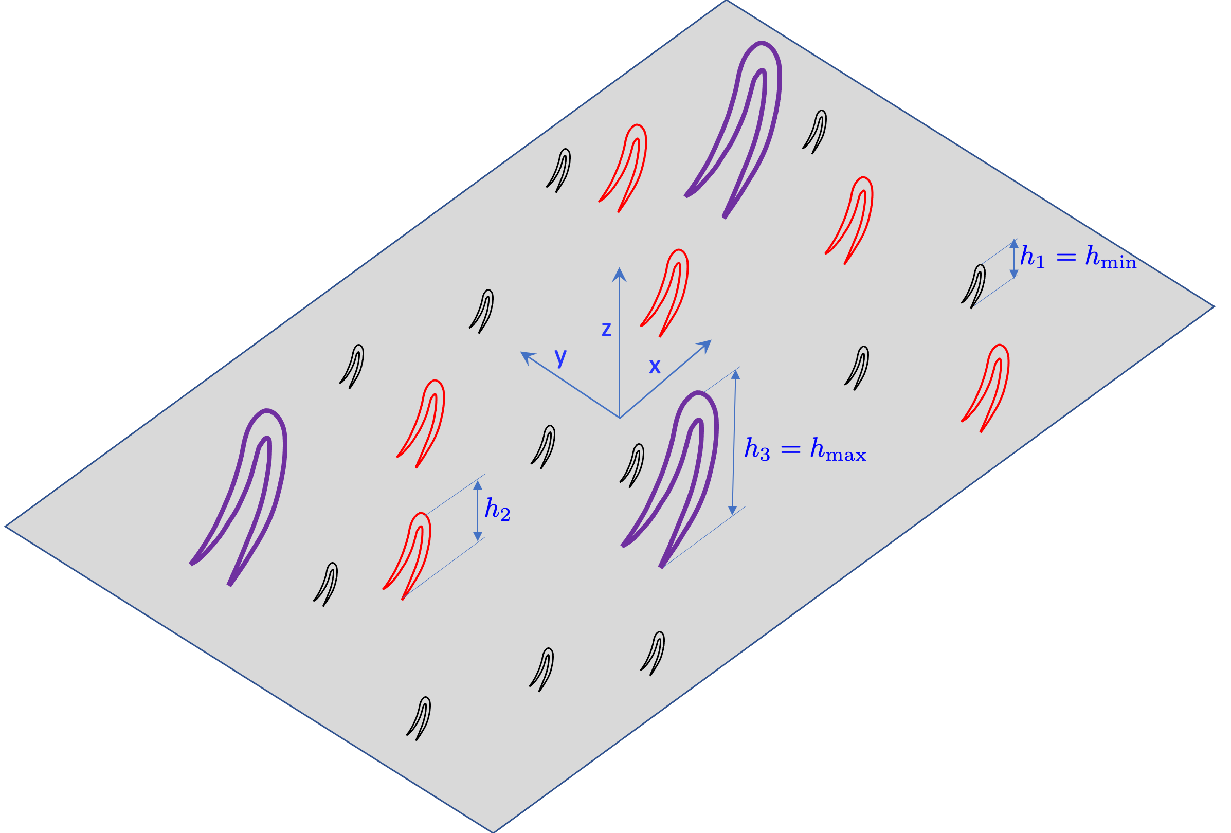
e

Figure 1: Schematic of discrete representation of attached eddies with $n=21$ and $m=3$.

Restricting our attention to a streamwise and spanwise square wall patch of side $2L$ in which the eddies are assumed to be idependently and uniformly distributed, and assuming that the range of eddy length scales follows a probability density function $p(h)$, the expectation of $q$ in this region is given by

$$q(\mathbf{x},n)\triangleq\mathbb{E}_{\mathbf{X}_{e},\mathbf{h}_{e}}[q(\mathbf{x},\mathbf{X}_{e},\mathbf{h}_{e},n)]=\frac{1}{4L^{2}}\int_{h_{min}}^{h_{max}}\int_{-L}^{L}\int_{-L}^{L}\sum_{i=1}^{n}q\left(\frac{\mathbf{x}-\mathbf{x}_{e,i}}{h}\right)p(h)d\mathbf{x}_{e,i}dh.$$ (1)

Homogenizing in the $x,y$ directions, assuming $L$ is large enough that each eddy centered at the origin has a negligible induced contribution outside an area $4L^{2}$ (Refer Campbell’s theorem  Rice (1944) and appendix of W&M), it can be shown that

$$q(z,n)\triangleq\mathbb{E}_{x,y}[q(\mathbf{x},n)]\approx\frac{n}{4L^{2}}\int_{h_{min}}^{h_{max}}\int_{-L}^{L}\int_{-L}^{L}q\left(\frac{\mathbf{x}}{h}\right)p(h)dxdydh.$$

Note that in the above equation, the entire field is written as a function of one prototypical eddy, which is scaled by the probability density function of the eddy sizes $p(h)$ and the eddy density $n/(4L^{2})$. If the mean eddy density is $\beta$, then using Poisson’s law, the expected value (over all numbers of eddies) is

$$Q(z)\triangleq\mathbb{E}_{n}[q(z,n)]=\beta\int_{h_{min}}^{h_{max}}\int_{-L}^{L}\int_{-L}^{L}q\left(\frac{\mathbf{x}}{h}\right)p(h)dxdydh.$$ (2)

Note that all the $q$’s defined above are random variables, yet $Q(z)$ is a deterministic quantity. Now we are in a position to define the mean streamwise velocity $U(z)$ as a superposition of eddies of various sizes $h$. This can be written in terms of the induced velocity field $u_{1}(\cdot)$ of one prototypical eddy.

$$U(z) \triangleq\beta\int_{h_{min}}^{h_{max}}\int_{-L}^{L}\int_{-L}^{L}u_{1}\left(\frac{\mathbf{x}}{h}\right)p(h)dxdydh+U_{\infty}$$

$$=\beta\int_{h_{min}}^{h_{max}}p(h)h^{2}\left[\int_{-L/h}^{L/h}\int_{-L/h}^{L/h}u_{1}\left(\frac{\mathbf{x}}{h}\right)d\left(\frac{x}{h}\right)d\left(\frac{y}{h}\right)\right]dh+U_{\infty}$$

$$=\beta\int_{h_{min}}^{h_{max}}p(h)h^{2}I_{1}\left(\frac{z}{h}\right)dh+U_{\infty},$$ (3)

where the mean flow eddy contribution function is

$$I_{1}\left(\frac{z}{h}\right) \triangleq\int_{-L/h}^{L/h}\int_{-L/h}^{L/h}u_{1}\left(\frac{\mathbf{x}}{h}\right)d\left(\frac{x}{h}\right)d\left(\frac{y}{h}\right).$$ (4)

Similarly, we can define the Reynolds stress tensor as

$$R_{ij}(z) \triangleq\beta\int_{h_{min}}^{h_{max}}p(h)I_{ij}\left(\frac{z}{h}\right)dh,$$

$$\textrm{ where }I_{ij}\left(\frac{z}{h}\right) \triangleq\int_{-L/h}^{L/h}\int_{-L/h}^{L/h}u_{i}\left(\frac{\mathbf{x}}{h}\right)u_{j}\left(\frac{\mathbf{x}}{h}\right)d\left(\frac{x}{h}\right)d\left(\frac{y}{h}\right).$$

Note the presence of an additional freestream velocity in the definition of $U(z)$. This is required because we are working with induced velocity fluctuations. The final piece we need is the probability distribution of the eddy sizes. Using insight from Townsend (1976) and  Perry & Chong (1982), W&M propose that $p(h)\propto 1/h^{3}$ and thus $p(h)=\frac{2/h^{3}}{1/h_{\min}^{2}-1/h_{\min}^{2}}$, with the note that $h_{\max}=\delta$ (i.e.) the boundary layer thickness and $h_{\min}$ is set by the friction Reynolds number $Re_{\tau}$. For notational simplicity, all length and velocity scales should be assumed to be in wall units henceforth.

2   The ideal eddy contribution function and a practical model

We now address the following question: How should the ’perfect’ eddy contribution function look like? Townsend and Perry & Chong have provided insight into the behavior of the eddy distribution function, but the current objective is to be precise. Towards this end, consider a discrete set of eddy sizes $\tilde{\mathbf{h}}=\{h_{1},h_{2},h_{3},..,h_{m}\}=\{h_{\min},h_{\min}+\Delta h,h_{\min}+2\Delta h,..,h_{\max}\}$ and a similar discretization of the wall-normal coordinate $\tilde{\mathbf{z}}=\{z_{1},z_{2},z_{3},..,z_{m}\}=\{h_{\min},h_{\min}+\Delta h,h_{\min}+2\Delta h,..,h_{\max}\}$. Then, the discretized velocity moments are

$$U(z_{r};\mathbf{d}) =\beta\sum_{l=1}^{m}p(h_{l})\left[\sum_{q}\sum_{p}u_{1}\left(\frac{{x_{p},y_{q},z_{r}}}{h_{l}};\mathbf{d}\right)\left(\frac{\Delta x}{h_{l}}\right)\left(\frac{\Delta y}{h_{l}}\right)\right]\Delta h+U_{\infty}$$

$$R_{ij}(z_{r};\mathbf{d}) =\beta\sum_{l=1}^{m}p(h_{l})\left[\sum_{q}\sum_{p}u_{i}\left(\frac{{x_{p},y_{q},z_{r}}}{h_{l}};\mathbf{d}\right)u_{j}\left(\frac{{x_{p},y_{q},z_{r}}}{h_{l}};\mathbf{d}\right)\left(\frac{\Delta x}{h_{l}}\right)\left(\frac{\Delta y}{h_{l}}\right)\right]\Delta h.$$

This can be represented as a matrix vector product in the form $\mathbf{U}(\tilde{\mathbf{z}})-U_{\infty}=\mathbf{A}\mathbf{b},$ where $A_{ij}=I_{1}(z_{i}/h_{j})$ and $b_{i}=\beta p(h_{i})h_{i}^{2}\Delta h.$ We would now like to extract these coefficients. Towards this end, we define the eddy contribution function at selected locations, and interpolate for the values in other locations in a piecewise linear fashion. In other words

$$\mathbf{A}=\begin{bmatrix}I_{1}(1)&I_{1}(h_{1}/h_{2})&I_{1}(h_{1}/h_{3})&..&I_{1}(h_{1}/h_{m-1})&I_{1}(h_{1}/h_{m})\\ I_{1}(h_{2}/h_{1})&I_{1}(1)&I_{1}(h_{2}/h_{3})&..&I_{1}(h_{2}/h_{m-1})&I_{1}(h_{2}/h_{m})\\ ..&..&..&..&..&..\\ I_{1}(h_{m}/h_{1})&I_{1}(h_{m}/h_{2})&I_{1}(h_{m}/h_{3})&..&I_{1}(h_{m}/h_{m-1})&I_{1}(1)\end{bmatrix}$$

$$\triangleq\begin{bmatrix}c_{1}&c_{m+1}&c_{m+2}&..&c_{2m-2}&c_{2m-1}\\ c_{2}&c_{1}&I_{1}(h_{2}/h_{3})&..&I_{1}(h_{2}/h_{m-1})&I_{1}(h_{2}/h_{m})\\ ..&..&..&..&..&..\\ c_{m}&I_{1}(h_{m}/h_{2})&I_{1}(h_{m}/h_{3})&..&I_{1}(h_{m}/h_{m-1})&c_{1}\\ \end{bmatrix}.$$

The unknown $I_{1}(\cdot)$ values are then interpolated  from the nodal locations $\mathbf{c}$. Note that there are more unknowns ($2m$) than equations ($m$), and so while it is possible to determine the unknowns that lead to perfect match of a reference (DNS or experiment) velocity profiles, a choice has to be made on the problem formulation. We choose to define the following least norm problem:

$$\{\mathbf{c}_{\textrm{opt}},\beta_{\textrm{opt}}\}=\min_{\mathbf{c},\beta}||\mathbf{U}_{ref}(\tilde{\mathbf{z}})-U_{\infty}-\mathbf{A}\mathbf{b}||_{2}^{2}.$$

Figure 2 shows the optimal eddy contribution functions inferred from the channel flow data (Lee & Moser, 2015) at friction Reynolds number $Re_{\tau}\approx 5200$. Figure 3 confirms that the first and second velocity moments are perfectly reproduced.

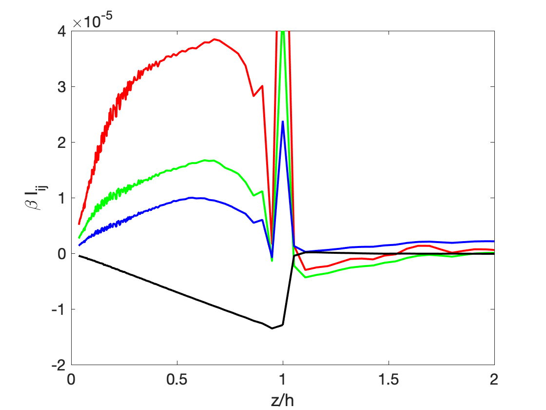
Figure 2: Optimal Influence functions for $Re_{\tau}\approx 5200$ for the mean flow (left) and Reynolds stresses (right, with red=streamwise; green=spanwise; blue=wall-normal, and black=shear).

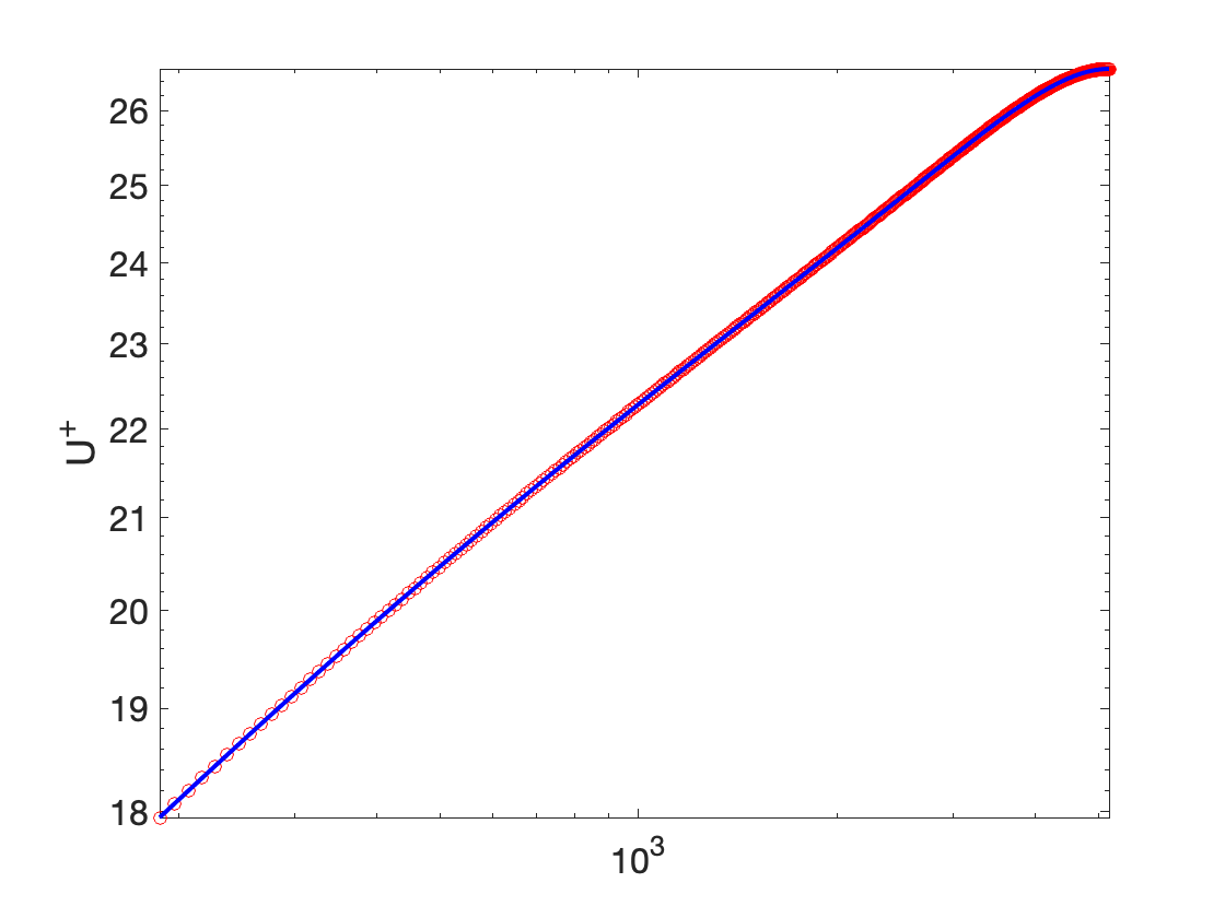
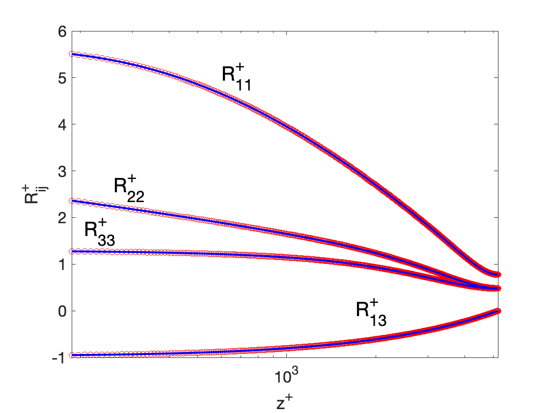
Figure 3: Reference (symbols) vs optimal attached eddy statistics for $Re_{\tau}\approx 5200$

Consider a collection of attached eddies that result in a simple function as shown in Fig. 4.

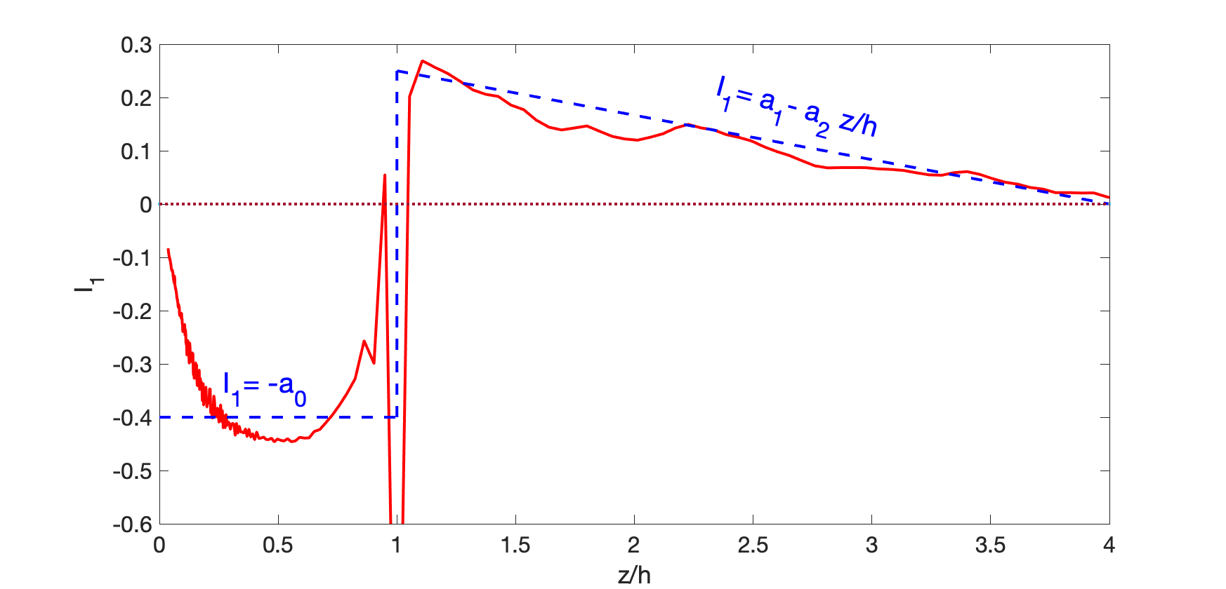
Figure 4: A hypothetical model of the eddy influence function corresponding to the mean streamwise velocity (blue dashed lines) compared to the optimal influence function.

It will be shown below that it is indeed possible to construct an attached eddy that corresponds to such a function. Using this influence function, one can reconstruct the mean streamwise velocity as

$$U(z) =\frac{2\beta}{1/h_{\min}^{2}-1/h_{\max}^{2}}\int_{h_{min}}^{h_{max}}\frac{I_{1}\left({z}/{h}\right)}{h}dh+U_{\infty}$$

$$=\frac{2\beta}{1/h_{\min}^{2}-1/h_{\max}^{2}}\int_{z/h_{max}}^{z/h_{min}}\frac{I_{1}\left({z}/{h}\right)}{z/h}d(z/h)+U_{\infty}$$

$$\approx\frac{2\beta}{1/h_{\min}^{2}-1/h_{\max}^{2}}\left[\int_{z/h_{max}}^{1}\frac{-a_{0}}{z/h}d(z/h)+\int_{1}^{a_{1}/a_{2}}\frac{a_{1}-a_{2}z/h}{z/h}d(z/h)\right]+U_{\infty}$$

$$=\frac{2\beta}{1/h_{\min}^{2}-1/h_{\max}^{2}}\left[\int_{z/h_{max}}^{1}\frac{-a_{0}}{z/h}d(z/h)+\int_{1}^{a_{1}/a_{2}}\frac{a_{1}-a_{2}z/h}{z/h}d(z/h)\right]+U_{\infty}$$

$$=\frac{2\beta}{1/h_{\min}^{2}-1/h_{\max}^{2}}\left[a_{0}\log[z/h_{\max}]+a_{1}\log[a_{1}/a_{2}]-a_{1}+a_{2}\right]+U_{\infty}.$$

It is thus clear that the Karman constant can be constructed as

$$\kappa=\frac{1/h_{\min}^{2}-1/h_{\max}^{2}}{2a_{0}\beta}.$$

Note that $W\&M$ use a Taylor series approximation on a generic eddy to derive an alternate expression for $\kappa$.

Now, we answer the question whether it is possible to recreate the above hypothetical influence function using an attached eddy. Consider a square hairpin (Figure 5) with unit circulation as the attached eddy, along with its image across the $z=0$ plane to enforce no-penetration. It is remarked that this eddy has a square structure, yet the leg of the eddy aligned with the wall is canceled by an equal and opposite image vortex pair, and is thus consistent with the kinematics. Using the Biot-savart law to compute the induced velocity $u_{1}$ in Eqn. 4, Figure 6 shows that such a simple attached eddy can reproduce the mean streamwise velocity extremely accurately. Further, the second moments are also seen to be reasonably well-predicted as shown in Figure 6.

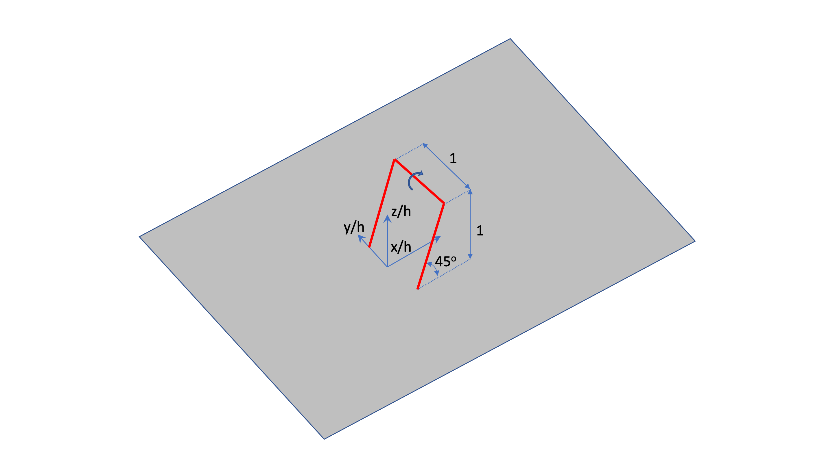
Figure 5: A prototypical hairpin-type eddy modeled using vortex line segments.

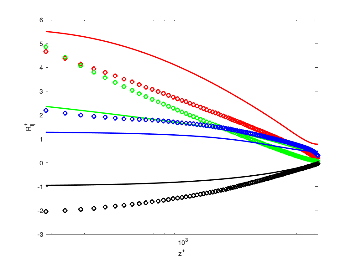
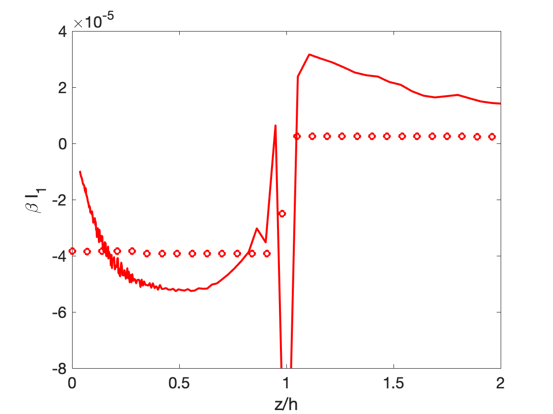
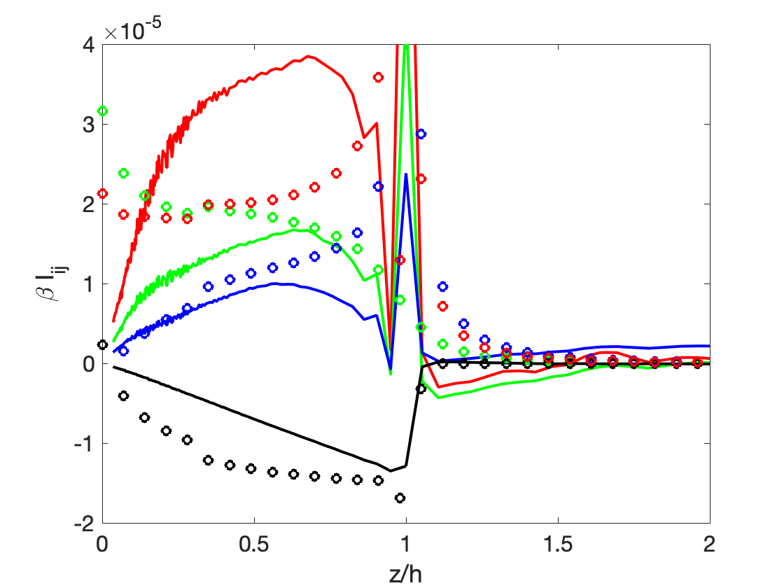
Figure 6: Velocity moments and eddy influence function. Lines: Optimal eddy influence function. Symbols: Square hairpin at $45^{\circ}$. For the right figures, colors follow Figure 2.

3   The optimal attached eddy

To assess whether the above attached eddy shape can be improved to yield more accurate statistics, we pose a constrained optimization problem. The prototypical attached eddy is now represented using 20 parameters as shown in Fig. 7. It is noted that the shape is symmetric across the $y=0$ plane, and a mirror image is used across the $z=0$ plane to satisfy inviscid boundary conditions.

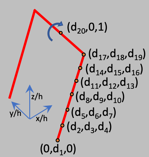
Figure 7: Representation of attached eddy using 20 parameters.

The following optimization problem is solved

$$\mathbf{d}_{\textrm{opt}} =\min_{\mathbf{d},\beta}(||\mathbf{U}_{ref}(\tilde{\mathbf{z}})-\mathbf{U}(\tilde{\mathbf{z}};\mathbf{d})||_{2}^{2}+||\mathbf{R}_{11,ref}(\tilde{\mathbf{z}})-\mathbf{R}_{11}(\tilde{\mathbf{z}};\mathbf{d})||_{2}^{2}+||\mathbf{R}_{22,ref}(\tilde{\mathbf{z}})-\mathbf{R}_{22}(\tilde{\mathbf{z}};\mathbf{d})||_{2}^{2}$$

$$+||\mathbf{R}_{33,ref}(\tilde{\mathbf{z}})-\mathbf{R}_{33}(\tilde{\mathbf{z}};\mathbf{d})||_{2}^{2}+||\mathbf{R}_{13,ref}(\tilde{\mathbf{z}})-\mathbf{R}_{13}(\tilde{\mathbf{z}};\mathbf{d})||_{2}^{2})$$

$$\textrm{s.t. }\mathbf{C}\mathbf{d}\leq\mathbf{f}\textrm{ and }\mathbf{d}_{l}\leq\mathbf{d}\leq\mathbf{d}_{u},$$

where the constraints $\mathbf{C}$ and $\mathbf{f}$ are designed to ensure that $d_{20}>d_{17}>d_{14}>d_{11}>d_{8}>d_{5}>d_{2}>0$, and $1>d_{19}>d_{16}>d_{13}>d_{10}>d_{7}>d_{4}>0$. The bounds $\mathbf{d}_{l},\mathbf{d}_{u}$ ensure that the x and y extents of the prototypical eddy is bounded. Sequential quadratic programming is used to solve the above constrained optimization problem. The results of the optimization is shown in Figures 8, 9, and improvement is noticeable over the simpler eddy (Figure 6) .

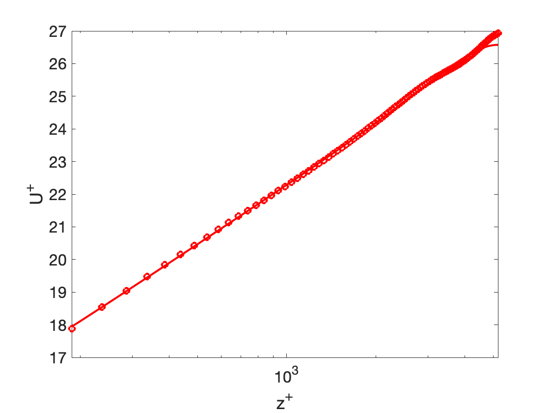
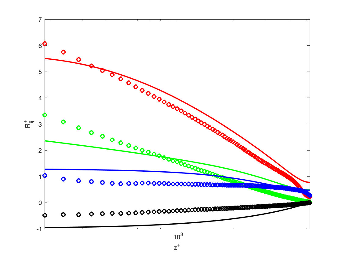
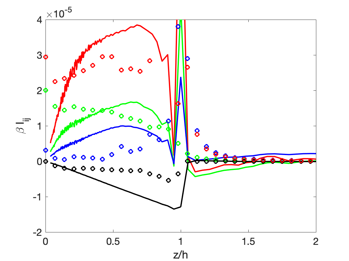
Figure 8: Velocity moments and eddy influence function. Lines: Optimal eddy influence function. Symbols: Optimal attached eddy. For the right figures, colors follow Figure 2.

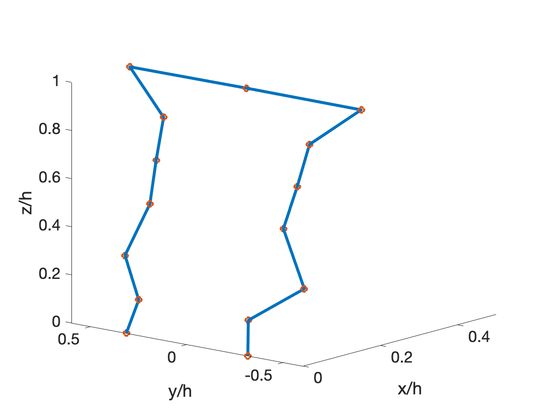
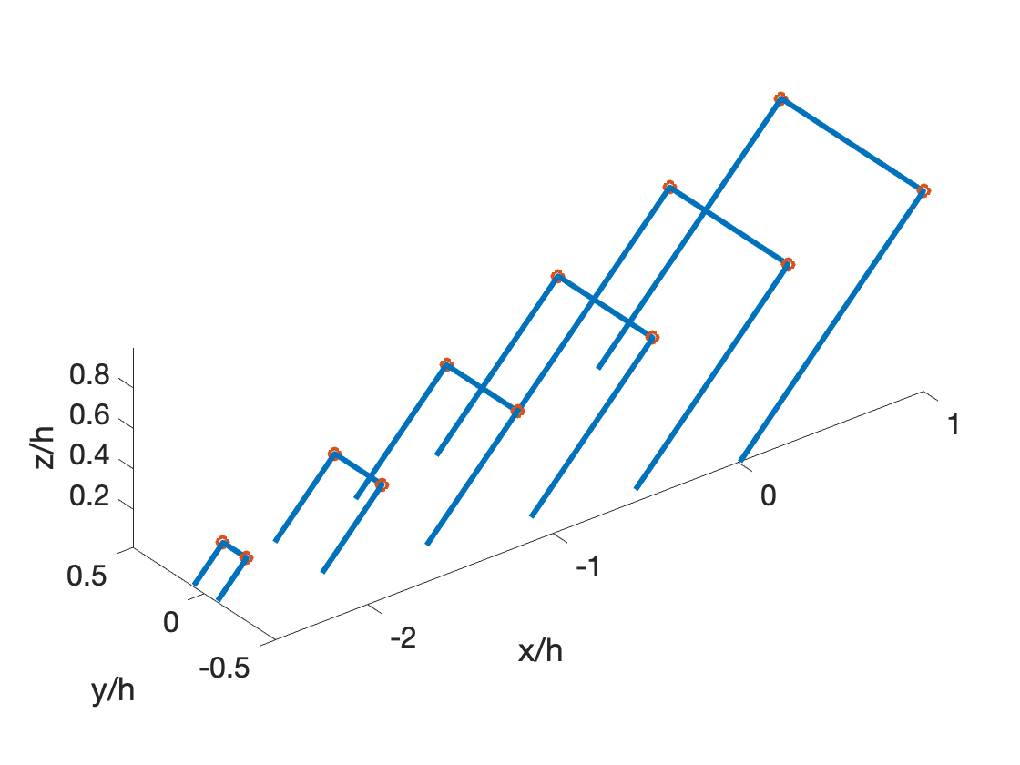
Figure 9: Prototypical eddies: Optimal attached eddy (left), Hairpin packet (right).

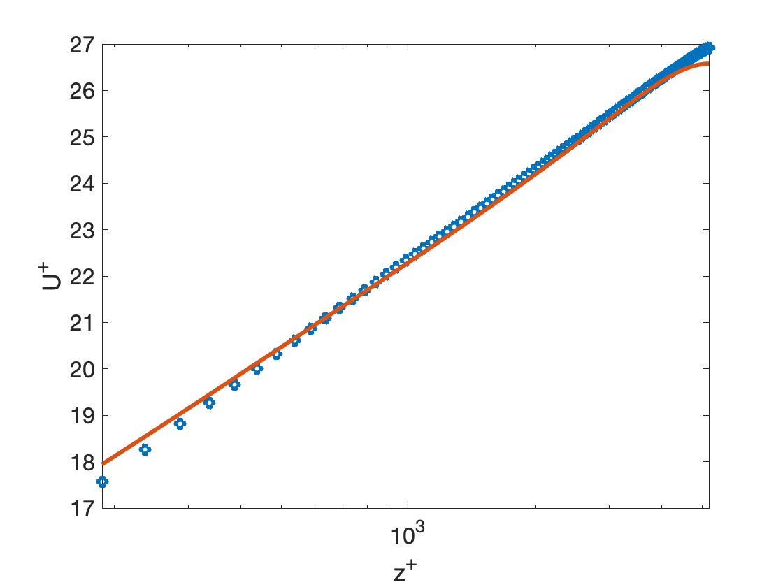
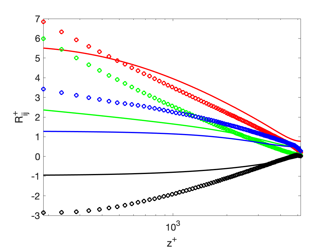
Figure 10: Velocity moments of optimal attached eddy packet (symbols) compared to DNS data. For the right figures, colors follow Figure 2.

At this juncture, we remark that the AEM is a statistical and non-dynamic model, and thus prototypical eddies cannot be considered to be physical structures. However, from a conceptual and aesthetic standpoint, the eddy shape in Figure 9 may be unsatisfactory. Indeed, analyses and observations from experiments and numerical simulations have suggested the following features of dynamically-important eddies: a) Hairpin-type structures are present the form of eddy packets (rather than individual eddies ), and b) A preferential alignment of approximately $45^{\circ}$ to the wall. Simply stacking the hairpins of Figure 5 with equal circulation strengths did not yield meaningful results, and thus the circulation strength of the individual hairpins in the packet (Figure 9) were optimized and found to follow a roughly quadratic distribution with hairpin size. It is noted that - in contrast to the above square hairpins, single / stacked lambda vortices did not yield accurate predictions of the statistics.

We conclude by stating that there are several directions for future work, including a) a more complete consideration of statistics such as the structure function, high-order moments, and the energy spectrum; b) assessment of the impact of the prototypical eddy in explaining physical characteristics of the flow; c) use of more sophisticated topological optimization and richer parametrizations of the eddies; and d) extension to other scenarios including boundary layers with pressure gradients and in combination with detached eddies. Further we note that opportunities exist in modeling flow regions beyond the log layer. In fact, the current inference approach and predictions already include the outer layer.

Acknowledgement This research was supported by NASA grant # 80NSSC18M0149 (Technical monitor: Dr. Gary Coleman).

Declaration of interests. The author reports no conflict of interest.

References

- Davidson & Krogstad (2009) Davidson, PA & Krogstad, P-Å 2009 A simple model for the streamwise fluctuations in the log-law region of a boundary layer. Physics of Fluids 21 (5), 055105.
- Davidson et al. (2006) Davidson, PA, Nickels, TB & Krogstad, P-Å 2006 The logarithmic structure function law in wall-layer turbulence. Journal of Fluid Mechanics 550, 51–60.
- Hwang & Eckhardt (2020) Hwang, Yongyun & Eckhardt, Bruno 2020 Attached eddy model revisited using a minimal quasi-linear approximation. Journal of Fluid Mechanics 894.
- Lee & Moser (2015) Lee, Myoungkyu & Moser, Robert D 2015 Direct numerical simulation of turbulent channel flow up to. Journal of fluid mechanics 774, 395–415.
- Lozano-Durán & Bae (2019) Lozano-Durán, Adrián & Bae, Hyunji Jane 2019 Characteristic scales of townsend’s wall-attached eddies. Journal of fluid mechanics 868, 698–725.
- Marusic & Monty (2019) Marusic, Ivan & Monty, Jason P 2019 Attached eddy model of wall turbulence. Annual Review of Fluid Mechanics 51, 49–74.
- Marusic et al. (2013) Marusic, Ivan, Monty, Jason P, Hultmark, Marcus & Smits, Alexander J 2013 On the logarithmic region in wall turbulence. Journal of Fluid Mechanics 716.
- McKeon (2019) McKeon, Beverley J 2019 Self-similar hierarchies and attached eddies. Physical Review Fluids 4 (8), 082601.
- Perry & Chong (1982) Perry, AE & Chong, MS 1982 On the mechanism of wall turbulence. Journal of Fluid Mechanics 119, 173–217.
- Perry & Marušić (1995) Perry, AE & Marušić, Ivan 1995 A wall-wake model for the turbulence structure of boundary layers. part 1. extension of the attached eddy hypothesis. Journal of Fluid Mechanics 298, 361–388.
- Rice (1944) Rice, Stephen O 1944 Mathematical analysis of random noise. The Bell System Technical Journal 23 (3), 282–332.
- de Silva et al. (2016a) de Silva, Charitha M, Hutchins, Nicholas & Marusic, Ivan 2016a Uniform momentum zones in turbulent boundary layers. Journal of Fluid Mechanics 786, 309–331.
- de Silva et al. (2016b) de Silva, Charitha M, Woodcock, James D, Hutchins, Nicholas & Marusic, Ivan 2016b Influence of spatial exclusion on the statistical behavior of attached eddies. Physical Review Fluids 1 (2), 022401.
- Townsend (1976) Townsend, AAR 1976 The structure of turbulent shear flow. Cambridge university press.
- Woodcock & Marusic (2015) Woodcock, JD & Marusic, I 2015 The statistical behaviour of attached eddies. Physics of Fluids 27 (1), 015104.