Bell nonlocality in classical systems

Abstract

The realistic interpretation of classical theory assumes that every classical system has well-defined properties, which may be unknown to the observer but are nevertheless part of reality and can in principle be revealed by measurements. Here we show that this interpretation can in principle be falsified if classical systems coexist with other types of physical systems. To make this point, we construct a toy theory that (i) includes classical theory as a subtheory and (ii) allows classical systems to be entangled with another type of systems, called anti-classical. We show that our toy theory allows for the violation of Bell inequalities in two-party scenarios where one of the settings corresponds to a local measurement performed on a classical system alone. Building on this fact, we show that measurements outcomes in classical theory cannot, in general, be regarded as pre-determined by the state of an underlying reality.

Introduction.

Since the early days of Galileo and Newton, classical theory has been regarded as the golden standard of a physical theory that describes reality without any fundamental uncertainty. In this view, every classical system is assumed to be in a well-defined state, which may be unknown to the observer, but is nevertheless part of the physical reality. Statistical mixtures only arise from the observer’s ignorance about the true state of the system, and in principle this ignorance can always be overcome by performing measurements. In modern terminology, the view that classical systems are fundamentally in well-defined (pure) states can be summarized by the statement that classical pure states are ontic, while classical mixed states are epistemic Hardy (2004); Spekkens (2005); Leifer (2014). This statement, combined with the idea that classical measurements reveal some pre-existing properties of the measured systems, lies at the core of the realistic interpretation of classical theory.

In this Letter we show that, contrarily to widespread belief, a realistic interpretation of classical theory is not always logically possible: while such interpretation is consistent with all experiments involving only classical systems, it can become in principle falsifiable if classical systems are considered alongside other types of physical systems. To make this point, we construct a toy theory that includes classical theory as a subtheory, meaning that it coincides with classical theory when restricted to a subset of the possible physical systems. In addition to all classical systems, the toy theory includes another type of systems, called anti-classical, as illustrated in Fig. 1. An observer who has access only to classical systems cannot see any difference between classical theory and our toy theory: all measurements are in principle compatible, all pure states are perfectly distinguishable through measurements, and all the states of all composite systems are separable. In contrast, we show that observers with joint access to both types of systems can in principle observe nonclassical features such as Bell nonlocality Brunner et al. (2014).

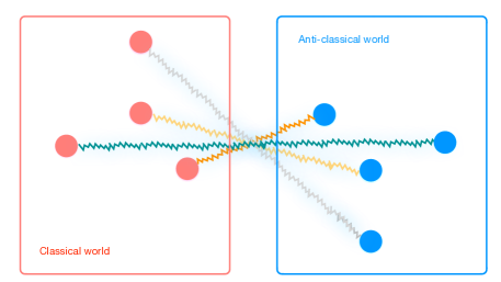
Figure 1: In a universe described by our toy theory, an observer who has access only to classical systems (represented by red disks on the left) would see a world described by classical theory. The same situation applies to an observer with access only to anti-classical systems (blue disks on the right). In contrast, observers with access to both types of systems can observe Bell nonlocality and other non-classical features.

Crucially, we show that our toy theory allows for a maximal violation of the Clauser-Horne-Shimony-Holt (CHSH) inequality Clauser et al. (1969); Cleve et al. (2004) in scenarios where where one of the settings corresponds to a local measurement performed on a classical system. Building on this result, we prove that measurement outcomes in classical theory cannot, in general, be regarded as pre-determined. Finally, we show that, under mild assumptions, the predictions of our toy theory cannot be reproduced by any deeper theory that describes reality as a list of individual properties of classical and anti-classical systems. This result indicates that, no matter whether the properties of classical systems are accessible through measurements or not, their full specification is not sufficient, in general, to account for the correlations between classical systems and other types of physical systems.

While our toy theory is not meant to be a description of the world, it makes an important conceptual point: the realistic interpretation of classical theory can in principle be falsified if classical systems exist alongside other types of physical systems. Notably, our toy theory cannot be ruled out from within classical theory: every classical phenomenon is in principle compatible with the existence of some yet-unobserved type of system that prevents the assignment of definite values to classical variables prior to measurement.

Our results complement recent works by Gisin and Del Santo Gisin (2019); Del Santo and Gisin (2019), who challenged the determinism of classical physics on the ground of the impossibility to specify real-valued variables like position and momentum with infinite precision. In our work, the impossibility to assign a pre-defined value to classical variables arises from correlations with some other physical systems, rather than precision limits in the definition of real numbers. As such, our results apply also to classical bits and other discrete classical variables. It is also worth mentioning that physical arguments in favour of classical indeterminism could also be put forward by setting up a dynamical interaction between classical and quantum systems (see e.g. Blanchard and Jadczyk (1995); Diosi (1995); Oppenheim (2023).) In the existing frameworks, however, classical and quantum systems cannot be entangled, and therefore there cannot be any CHSH violation when one of the settings corresponds to a measurement on a classical system alone. In this respect, our toy theory exhibits a stronger form of indeterminism.

Classical and anti-classical systems.

To formulate our toy theory we adopt the framework of general probabilistic theories Hardy (2001); Barrett (2007); Barnum et al. (2007); Hardy (2011a, 2013a, 2016), in the specific version known as operational probabilistic theories (OPTs) Chiribella et al. (2010a, 2011); Perinotti et al. (2016); Chiribella et al. (2016); Hardy (2013b); Scandolo (2018). An OPT describes a set of physical systems, closed under composition, and a set of transformations thereof, closed under parallel and sequential composition. Mathematically, the compositional structure is underpinned by the graphical language of process theories Abramsky and Coecke (2004, 2008); Coeke (2010); Coecke and Kissinger (2017).

Classical theory can be regarded as a special case of an OPT Hardy (2011a); Scandolo et al. (2021): precisely, it is the largest OPT where (i) the pure states of every given system are perfectly distinguishable through a single measurement, (ii) the pure states of every composite system are the products of pure states of the component systems, and (iii) all permutations of the set of pure states are valid physical transformations. For simplicity, we will focus on the classical theory of discrete systems such as bits and their generalizations.

We now construct a toy theory that includes classical theory as a subtheory, meaning that our toy theory coincides with classical theory when restricted to a subset of physical systems that includes all discrete classical systems. A classical system with $d$ perfectly distinguishable pure states, conventionally denoted by $0,1,\dots,d-1$, will be called a dit (or a bit in the special case $d=2$.) The mixed states of a dit are probability distributions of the form $(p_{i})_{i=0}^{d-1}$, with $p_{i}\geq 0\,,\forall i$ and $\sum_{i=0}^{d-1}p_{i}=1$. The reversible processes acting on the dit are permutations of its pure states, while general noisy processes are described by transition probabilities $p(j|i)$. Similarly, a (generally noisy) measurement with outcomes in a set $\sf A$ can be represented by transition probabilities $p(a|i)$, yielding the probability of the outcome $a$ when the dit is in the state $i$.

An equivalent way to represent classical states, processes, and measurements, commonly used in the quantum information literature (see e.g. Heinosaari and Ziman (2011)), is provided by diagonal matrices. Specifically, probability distributions $(p_{i})_{i=0}^{d-1}$ can be equivalently represented by $d\times d$ diagonal matrices of the form $\rho=\sum_{i=0}^{d-1}p_{i}|i\rangle\langle i|$, where $\{|i\rangle\}_{i=0}^{d-1}$ is the canonical orthonormal basis for $\mathbb{C}^{d}$. A general process with transition probabilities $p(j|i)$ is described by a linear map of the form $\mathcal{M}(\rho)=\sum_{i,j}\,p(j|i)\,|j\rangle\langle j|\,\langle i|\rho|i\rangle$. Finally, a measurement with outcomes in the set $\sf A$ is described by a positive operator-valued measure (POVM) $(P_{a})_{a\in\sf A}$ of the form $P_{a}=\sum_{i=0}^{d-1}\,p(a|i)\,|i\rangle\langle i|$, and the outcome probabilities can be computed with the Born rule $p(a|i)=\langle i|P_{a}|i\rangle$.

In our toy theory, classical systems coexist with another type of systems, called anti-classical. The anti-classical systems can be viewed as a mirror image of the classical systems: for every classical system type, there exists a corresponding anti-classical system type with exactly the same state space, the same set of physical transformations, and the same set of measurements. To help intuition, one can think of the distinction between classical and anti-classical systems as analogous to the distinction between particles and anti-particles, which have the same state spaces, and yet are distinguishable by some external property, such as their charge.

While classical and anti-classical systems are described by classical probability theory when considered separately, composite systems including both types of systems exhibit non-classical features. In the following, we present the simplest version of our toy theory, which describes arbitrary composite systems made of $m$ bits and $n$ anti-bits, herafter called $(m,n)$-composites. $(m,0)$ and $(0,n)$ composites will be described by classical theory, while the non-classical behaviours will emerge when both $m$ and $n$ are non-zero. The generalization to basic systems of arbitrary dimension, as well as the full specification of the allowed states, measurements, and processes, is provided in the Supplemental Material sup .

Non-classical composites.

The simplest non-classical composite is the $(1,1)$-composite, consisting of a bit and an anti-bit. In this case, the pure states are represented by rank-one projectors onto unit vectors $|\Psi\rangle$ with well-defined parity, that is, unit vectors satisfying either the condition $\Pi_{0}|\Psi\rangle=|\Psi\rangle$ or the condition $\Pi_{1}|\Psi\rangle=|\Psi\rangle$, where $\Pi_{0}$ ($\Pi_{1}$) is the projector on the subspace spanned by the vectors $\{|0\rangle|0\rangle,|1\rangle|1\rangle\}$ ($\{|0\rangle|1\rangle,|1\rangle|0\rangle\}$). The mixed states of a bit and an anti-bit are described by density matrices of the form $\rho=\sum_{j}\,q_{j}\,|\Psi_{j}\rangle\langle\Psi_{j}|$, where $(|\Psi_{j}\rangle)_{j}$ are pure states and $(q_{j})_{j}$ is a probability distribution. For an $(m,m)$-composite, the most general pure state is a unit vector of the form $|\Psi\rangle=\left[I_{(B_{1}\dots B_{m})}\otimes U^{(A_{1}\dots A_{m})}\right]\,|\Psi^{\prime}\rangle$, where $U^{(A_{1}\dots A_{m})}$ is a unitary operator that permutes $m$ bits (anti-bits) and $|\Psi^{\prime}\rangle$ is a unit vector satisfying the condition

$$|\Psi^{\prime}\rangle=\left(\Pi_{k_{1}}^{B_{1}A_{1}}\otimes\cdots\otimes\Pi^{B_{m}A_{m}}_{k_{m}}\right)\,|\Psi^{\prime}\rangle\,,$$ (1)

for given vector $(k_{1},\dots,k_{m})\in\{0,1\}^{\times m}$, where we used the notation $\Pi^{B_{i}A_{i}}_{k_{i}}$ for the projector onto the subspace of the composite system of the $i$-th bit and $i$-th anti-bit with fixed parity $k_{i}\in\{0,1\}$.

The pure states of arbitrary $(m,n)$-composites are defined in the Supplemental Material sup . General mixed states are defined as density matrices that are convex combinations of rank-one density matrices associated with the above pure states. Measurements on system $S$ are defined as POVMs $\{P_{i}\}_{i=1}^{k}$ whose operators are linear combinations, with positive coefficients, of the allowed states, and satisfy the normalization property $\sum_{i=1}^{k}P_{i}=I_{S}$. The outcome probabilities are then given by the Born rule $p_{i}=\Tr[P_{i}\rho]$. With these definitions, states and measurements satisfy a fundamental consistency condition: when a subset of the systems is measured, the conditional states of the remaining systems is still a valid state allowed by our toy theory. We call this condition consistency of the conditional states and prove it in the Supplemental Material sup , where we also show that similar consistency properties hold for all processes in our toy theory. In particular, all the multipartite states, processes, and measurements allowed by our toy theory coincide with the states, processes, and measurements of classical theory once all the anti-classical systems are eliminated.

It is worth noting that, unlike classical theory and standard quantum theory on the complex field, our toy theory does not satisfy Local Tomography Araki (1980); Wootters (1990); Hardy (2001); Barrett (2007); D’ariano et al. (2010); Chiribella et al. (2010b); Hardy (2011b), the property that the states of composite systems are completely characterized by the correlations of local measurements. While this property holds separately for all classical systems and for all anti-classical systems, it fails to hold when classical and anti-classical systems are combined together.

The violation of Local Tomography is not an accident, but rather a necessary condition for obtaining non-classical composites out of systems with classical state spaces D’Ariano et al. (2020) (see also the no-go theorem in Aubrun et al. (2021) where local tomography is implicit in the choice of possible tensor products). Nevertheless, we show that our toy theory satisfies a weaker locality property, known as Bilocal Tomography Hardy and Wootters (2012), for all multipartite systems consisting of bits and anti-bits: any arbitrary state of $m$ bits and $n$ anti-bits can be fully characterized by the correlations of measurements performed on pairs of bits and anti-bits. A proof of this fact is provided in the Supplemental Material sup . Other examples of physical theories that violate Local Tomography but satisfy Bilocal Tomography are quantum theory on real vector spaces Araki (1980); Wootters (1990), Fermionic quantum theory D’Ariano et al. (2014); Vidal et al. (2021), and doubled quantum theory  Chiribella and Scandolo (2017); Scandolo (2018).

Classical mixtures from entanglement.

It is immediate to see that every mixed state of a classical bit can be obtained from a pure state of the composite system by discarding the anti-bit. For example, the generic mixed state $\rho=p\,|0\rangle\langle 0|+(1-p)\,|1\rangle\langle 1|$ can be obtained from the pure entangled state $|\Psi\rangle=\sqrt{p}\,|0\rangle|0\rangle+\sqrt{1-p}\,|1\rangle|1\rangle$. In other words, every mixed state of a classical bit admits a purification Chiribella et al. (2010b); Perinotti et al. (2016).

In the rest of the paper we discuss the implications of purification for the interpretation of classical physics. Let us first assume, for the sake of argument, that our toy theory describes nature at the fundamental (i.e. ontic) level. In this setting, the claim that every classical system must be in a pure state at the ontic level would imply that the joint states of a bit/anti-bit pair are always of the separable form $\Sigma=q\,|0\rangle\langle 0|\otimes\rho_{0}+(1-q)\,|1\rangle\langle 1|\otimes\rho_{1}$, for some probability $q\in[0,1]$ and some states $\rho_{0}$ and $\rho_{1}$ of the anti-bit (see Supplemental Material sup ). But this condition is manifestly in contradiction with the existence of pure entangled states. Operationally, any pure entangled state of a bit/anti-bit pair can be distinguished from all separable states by performing a measurement allowed by the toy theory. For example, the pure entangled state $|\Psi\rangle=\sqrt{p}\,|0\rangle|0\rangle+\sqrt{1-p}\,|1\rangle|1\rangle$, $p\in(0,1)$, can be distinguished with a guaranteed success probability of at least $\min\{p,1-p\}$ from all separable states (see Supplemental Material sup ). Hence, we conclude that, in a world where our toy theory is fundamental, the belief that classical systems must always be in some (possibly unknown) pure states can be experimentally falsified.

Bell nonlocality.

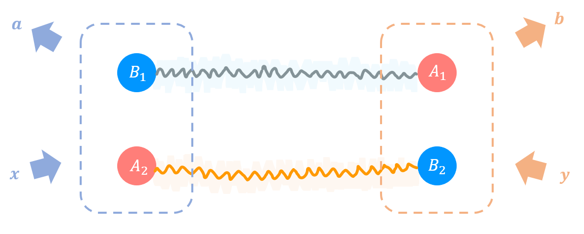
Figure 2: Activation of Bell nonlocality with bit/anti-bit entangled pairs. Alice (left) and Bob (right) perform local measurements on two copies of an entangled state of a bit/anti-bit pair. The first copy (top) involves bit $B_{1}$ and anti-bit $A_{1}$, while the second copy (bottom) involves bit $B_{2}$ and anti-bit $A_{2}$. Alice’s and Bob’s laboratories (represented dotted boxes) contain systems $B_{1}A_{2}$ and $A_{2}B_{1}$, respectively. Their measurements have settings $x$ and $y$, respectively, and produce outcomes $a$ and $b$, respectively.

We now use our toy theory to challenge the common belief that the outcomes of classical measurements reveal the values of some pre-existing properties of the measured systems. The starting point of our argument is the observation that our toy theory exhibits activation of Bell nonlocality Peres (1996); Masanes et al. (2008); Cavalcanti et al. (2011); Navascués and Vértesi (2011); Palazuelos (2012). Suppose that a bit $B$ and an anti-bit $A$ are in the entangled state $|\Phi\rangle_{BA}=(|0\rangle_{B}|0\rangle_{A}+|1\rangle_{B}|1\rangle_{A})/\sqrt{2}$. This state alone does not give rise to any Bell inequality violation: since the local measurements on a bit and anti-bit are classical, one can easily construct a local hidden variable model. However, Bell nonlocality arises when we consider the two-copy state $|\Phi\rangle_{B_{1}A_{1}}\otimes|\Phi\rangle_{B_{2}A_{2}}$, where $B_{1}B_{2}$ are bits, and $A_{1}A_{2}$ are anti-bits. Suppose that two parties, Alice and Bob, play a nonlocal game, such as the CHSH game Clauser et al. (1969); Cleve et al. (2004), in the scenario where Alice has access to system $B_{1}A_{2}$, while Bob has access to system $B_{2}A_{1}$, as illutrated in Fig. 2.

We now show that the state $|\Phi\rangle_{B_{1}A_{1}}\otimes|\Phi\rangle_{B_{2}A_{2}}$ allows Alice and Bob to reproduce the correlations of arbitrary single-qubit measurements performed locally on a two-qubit maximally entangled state. More specifically, we show that a qubit measurement that projects Alice’s qubit on a given orthonormal basis $\left\{|v_{0}\rangle,|v_{1}\rangle\right\}$ with $|v_{0}\rangle=\alpha\,|0\rangle+\beta\,|1\rangle$ can be simulated by a measurement on the bit/anti-bit pair $B_{1}A_{2}$, described by two orthogonal projectors $\{P_{0},P_{1}\}$ with

$$P_{0}= |V^{(0)}_{0}\rangle\langle V^{(0)}_{0}|_{B_{1}A_{2}}+|V^{(1)}_{0}\rangle\langle V^{(1)}_{0}|_{B_{1}A_{2}}$$

$$\quad|V^{(0)}_{0}\rangle_{B_{1}A_{1}}=\alpha\,|0\rangle_{B_{1}}|0\rangle_{A_{2}}+\beta\,|1\rangle_{B_{1}}|1\rangle_{A_{2}}$$

$$\quad|V^{(1)}_{0}\rangle_{B_{1}A_{2}}=\alpha\,|0\rangle_{B_{1}}|1\rangle_{A_{2}}+\beta\,|1\rangle_{B_{1}}|0\rangle_{A_{2}}\,,$$ (2)

and $P_{1}=I_{B_{1}}\otimes I_{A_{2}}-P_{0}$, acting on the bit/anti-bit pair $B_{1}A_{2}$. Similarly, a measurement that projects Bob’s qubit on the orthonormal basis $\{|w_{0}\rangle,|w_{1}\rangle\}$ with $|w_{0}\rangle=\gamma|0\rangle+\delta|1\rangle$ can be simulated by the projective measurement $\{Q_{0},Q_{1}\}$ defined by

$$Q_{0}= |W^{(0)}_{0}\rangle\langle W^{(0)}_{0}|_{B_{2}A_{1}}+|W^{(1)}_{0}\rangle\langle W^{(1)}_{0}|_{B_{2}A_{1}}$$

$$\quad|W^{(0)}_{0}\rangle=\gamma\,|0\rangle_{B_{2}}|0\rangle_{A_{1}}+\delta\,|1\rangle_{B_{2}}|1\rangle_{A_{1}}$$

$$\quad|W^{(1)}_{0}\rangle=\gamma\,|1\rangle_{B_{2}}|0\rangle_{A_{1}}+\delta\,|0\rangle_{B_{2}}|1\rangle_{A_{1}}\,,$$ (3)

and $Q_{1}=I_{B_{2}}\otimes I_{A_{1}}-Q_{0}.$ When these measurements are performed on the state $\rho=|\Phi\rangle\langle\Phi|_{B_{1}A_{1}}\otimes|\Phi\rangle\langle\Phi|_{B_{2}A_{2}}$, Alice and Bob obtain outcomes $a$ and $b$ with probability

$$p(a,b)=\Tr[(P_{a}\otimes Q_{b})\,\rho]\equiv\left|\langle v_{a}|\langle w_{b}|\,|\Phi\rangle\right|^{2}\,,$$ (4)

equal to the outcome probability of the original single-qubit measurements performed on the two-qubit maximally entangled state $|\Phi\rangle$ (see the Supplemental Material for more details). In this way, every pair of local measurements on a maximally entangled two-qubit quantum state can be simulated by local measurements in our toy theory. In particular, Alice and Bob can simulate the optimal strategy in the CHSH game Clauser et al. (1969); Cleve et al. (2004); Tsirel’son (1980, 1987), thereby achieving a maximal violation of the CHSH inequality.

Let us now examine the implications of the above result for the interpretation of classical theory. A first, important consequence is that the value of Alice’s classical bit cannot, in general, be regarded as pre-determined. This conclusion follows from the fact that the violation of the CHSH inequality can be achieved with by setup in which one of Alice’s measurements is the canonical measurement on bit $B_{1}$. Technically, this follows from the fact that one of Alice’s measurements in the original quantum scenario is a qubit measurement on the computational basis $\{|0\rangle,|1\rangle\}$. In our simulation, this measurement corresponds to the projectors $P_{0}=|0\rangle\langle 0|_{B_{1}}\otimes I_{A_{2}}$ and $P_{1}=I\otimes I-P_{0}=|1\rangle\langle 1|_{B_{1}}\otimes I_{A_{2}}$, as one can see from Eq. (2). Operationally, this measurement is realized by discarding the anti-bit $A_{2}$, and measuring bit $B_{1}$ on the basis $\{|0\rangle,|1\rangle\}$. Since Alice’s bit value is a measurement outcome in a setup that violates the CHSH inequality, we conclude that the bit value cannot be predetermined Barrett et al. (2006): explicitly, in the Supplemental Material we show that, if the underlying ontic state determines the value of Alice’s bit up to an error $\epsilon$, then the CHSH value cannot exceed $2(1+2\epsilon)$ and therefore cannot reach the maximum value $2\sqrt{2}$ when $\epsilon$ is small. In the Supplemental Material we also show that the above argument applies to all pure entangled states of a dit and an anti-dit sup .

Another implication of Bell nonlocality is that, even if we replace our toy theory with a more fundamental description of nature, this description cannot, under reasonable assumptions, assign individual ontic states to classical systems. Two different argument leading to this conclusion are provided in the Supplemental Material sup . In both cases, the conclusion is that classical systems in our toy theory cannot be reduced to independent and uncorrelated degrees of freedom of the underlying reality.

Conclusions.

In this work we have shown that the realistic interpretation of classical theory can in principle be falsified when classical systems coexist with other types of physical systems. We built a toy theory in which every classical system can be entangled with a dual, anti-classical system. The entanglement between classical and anti-classical systems gives rise to activation of Bell nonlocality and implies that, in general, the outcomes of measurements on classical systems cannot be interpreted as revealing the values of some pre-existing properties of the measured systems.

I SUPPLEMENTAL MATERIAL

II Toy theory with basic systems of arbitrary dimension

We now provide a generalization of our toy theory to the scenario where the basic systems have general dimension $d\geq 2$.

II.1 Systems

A classical (anti-classical) system with $d$ perfectly distinguishable pure states, named dit (anti-dit), is denoted by the letter $D$ ($A$) and is assigned to a $d$-dimensional Hilbert space $\mathcal{H}_{D}\simeq\mathbb{C}^{d}$ ($\mathcal{H}_{A}\simeq\mathbb{C}^{d}$). In the following we will consider composite systems where the dimension $d$ of the elementary systems is fixed. In other words, we consider composite systems consisting of a given number $m$ of dits and a given number $n$ of anti-dits of given dimension $d$. The resulting composite system will be denoted by the pair $(m,n)$ and we will be called a system of type $(m,n)$.

A composite system $S$ consisting of $m$ dits $D_{1}\cdots D_{m}$ and $n$ anti-dits $A_{1}\cdots A_{n}$ will be associated to the Hilbert space

$$\mathcal{H}_{S}\mathrel{\mathop{\ordinarycolon}}=\mathcal{H}_{D_{1}}\otimes\cdots\otimes\mathcal{H}_{D_{m}}\otimes\mathcal{H}_{A_{1}}\otimes\cdots\otimes\mathcal{H}_{A_{n}}\simeq\left(\mathbb{C}^{d}\right)^{\otimes m}\otimes\left(\mathbb{C}^{d}\right)^{\otimes n}\,.$$ (5)

In the following, we will denote by $\mathsf{Lin}(\mathcal{H}_{S})$ (or simply $\mathsf{Lin}(S)$) the vector space of all linear operators on $\mathcal{H}_{S}$. The states of system $S$ will be described by a suitable subset of the operators in $\mathsf{Lin}(\mathcal{H}_{S})$.

II.2 Pure states

We now specify the pure states of composite systems of type $(m,n)$, for all possible values of $m$ and $n$. In all these cases, the pure states of a system $S$ are mathematically represented by suitable rank-one projectors, of the form $\rho=|\psi\rangle\langle\psi|$ for some unit vector $|\psi\rangle\in\mathcal{H}_{S}$ satisfying appropriate conditions. The set of pure states of system $S$ will be denoted by ${\mathsf{Pur}}{\mathsf{St}}(S)\subset\mathsf{Lin}(\mathcal{H}_{S})$. With a slight abuse of notation, common in presentations of quantum theory, we will sometime refer to the unit vector $|\psi\rangle$, rather than the corresponding projector, as a “pure state.”

II.2.1 Composites of type $(m,0)$ and $(n,0)$

All composites of this type obey the rules of classical theory, and their states are described by density matrices that are diagonal in a given basis, called the computational basis.

The pure states of a dit $D$ (anti-dit $A$) are $d\times d$ density matrices of the form $\rho=|i\rangle\langle i|$, where $\{|i\rangle\}_{i=0}^{d-1}$ is the computational basis for $\mathbb{C}^{d}$. In the following, we will use the short-hand notation

$$\mathbb{Z}_{d}\mathrel{\mathop{\ordinarycolon}}=\{0,\dots,d-1\}\,,$$ (6)

and will label the computational basis as $\{|i\rangle\}_{i\in\mathbb{Z}_{d}}$.

For composite systems consisting only of dits (i.e. systems of type $(m,0)$) or only of anti-dits (i.e. systems of type $(0,m)$), the allowed pure states are density matrices of the form $\rho=|{\mathbf{i}}\rangle\langle{\mathbf{i}|}$, where $\mathbf{i}=(i_{1},\dots,i_{m})$ is a vector with $m$ entries in $\mathbb{Z}_{d}$, and

$$|{\bf i}\rangle\mathrel{\mathop{\ordinarycolon}}=|i_{1}\rangle\otimes\cdots\otimes|i_{m}\rangle\,.$$ (7)

In the following, the set of vectors $(i_{1},\dots,i_{m})$ with $m$ entries in $\mathbb{Z}_{d}$ will be denoted by $\mathbb{Z}_{d}^{m}$.

II.2.2 Composites of type $(m,m)$

Let us start from the $(1,1)$ case. The composite system of a dit $D$ and an anti-dit $A$ is associated to the Hilbert space $\mathcal{H}_{DA}\mathrel{\mathop{\ordinarycolon}}=\mathcal{H}_{D}\otimes\mathcal{H}_{A}$, where $\mathcal{H}_{D}\simeq\mathbb{C}^{d}$ and $\mathcal{H}_{A}\simeq\mathbb{C}^{d}$ are the Hilbert spaces associated to $D$ and $A$, respectively. To specify the allowed pure states, we introduce a set of orthogonal subspaces, labelled by integers in $\mathbb{Z}_{d}$. For a given $q\in\mathbb{Z}_{d}$, we define the subspace

$$\mathcal{H}^{q}_{DA}\mathrel{\mathop{\ordinarycolon}}={\mathsf{Span}}\Big{\{}|i\rangle_{D}|i\oplus q\rangle_{A}\,,~{}i\in\mathbb{Z}_{d}\Big{\}}\subset\mathcal{H}_{DA}\,,$$ (8)

where $\oplus$ denotes the sum modulo $d$. The integer $q$ will be referred to as the type of the subspace. For $d=2$, the type $q\in\{0,1\}$ is simply the parity. Vectors in the subspace $\mathcal{H}_{DA}^{q}$ will be called vectors of type $q$.

We are now ready to define the pure states of the $(1,1)$ composites:

Definition 1.

The pure states of a dit/anti-dit composite $DA$ are projectors of the form $|\psi\rangle\langle\psi|$, where $|\psi\rangle$ is a unit vector of type $q$ for some $q\in\mathbb{Z}_{d}$. In formula,

$${\mathsf{Pur}}{\mathsf{St}}(DA)\mathrel{\mathop{\ordinarycolon}}=\bigcup_{q=\in\mathbb{Z}_{d}}{\mathsf{Pur}}{\mathsf{St}}(DA;q)\qquad{\rm with}\qquad{\mathsf{Pur}}{\mathsf{St}}(DA;q)\mathrel{\mathop{\ordinarycolon}}=\left\{|\psi\rangle\langle\psi|~{}\Big{|}~{}|\psi\rangle\in\mathcal{H}^{q}_{DA}\,,\|\,|\psi\rangle\,\|=1\right\}\,.$$ (9)

We call ${\mathsf{Pur}}{\mathsf{St}}(DA;q)$ the set of pure states of type $q$. Note that ${\mathsf{Pur}}{\mathsf{St}}(DA;q)$ coincides with the set of pure states of a quantum system of dimension $d$ (qudit). As we will see later in this Supplemental Material, the relation with quantum theory will play a key role in determining the properties of our toy theory.

In the special case of a dit and an anti-dit ($d=2$), the state space of the composite system is the direct sum of two orthogonal sectors, where each sector is isomorphic to a qubit state space. A similar state space also appeared in earlier toy theories, such as Fermionic theory D’Ariano et al. (2014); Vidal et al. (2021), doubled quantum theory  Chiribella and Scandolo (2017); Scandolo (2018), and extended classical theory Scandolo (2018). These theories, however, differ from our toy theory in the definition of multipartite composites with more than two components, and, most importantly, do not contain the whole classical theory as a subtheory.

Let us now consider the case of general $m\geq 1$. A composite of $m$ dits $D_{1}\dots D_{m}=\mathrel{\mathop{\ordinarycolon}}\mathbf{D}$ and $m$ anti-dits $A_{1}\dots A_{m}\mathrel{\mathop{\ordinarycolon}}=\mathbf{A}$ is associated to the Hilbert space $\mathcal{H}_{\mathbf{D}\mathbf{A}}\mathrel{\mathop{\ordinarycolon}}=\mathcal{H}_{\mathbf{D}}\otimes\mathcal{H}_{\mathbf{A}}$, where $\mathcal{H}_{\mathbf{D}}\mathrel{\mathop{\ordinarycolon}}=\mathcal{H}_{D_{1}}\otimes\cdots\otimes\mathcal{H}_{D_{m}}$ and $\mathcal{H}_{\mathbf{A}}\mathrel{\mathop{\ordinarycolon}}=\mathcal{H}_{A_{1}}\otimes\cdots\otimes\mathcal{H}_{A_{m}}$ are the Hilbert spaces associated to the dits $\mathbf{D}$ and to the anti-dits $\mathbf{A}$, respectively.

To define the pure states of the composite system $\mathbf{D}\mathbf{A}$, we pair every dit in $\mathbf{D}$ with an anti-dit in $\mathbf{A}$. The pairing is defined by a permutation $\pi\mathrel{\mathop{\ordinarycolon}}\{1,\dots,m\}\to\{1,\dots,m\}$, which associates the dit $D_{i}$ with an anti-dit $A_{\pi(i)}$ for every $i\in\{1,\dots,m\}$. We then define the subspaces

$$\mathcal{H}_{\mathbf{D}\mathbf{A}}^{\pi,\mathbf{q}}\mathrel{\mathop{\ordinarycolon}}=\mathcal{H}_{D_{1}A_{\pi(1)}}^{q_{1}}\otimes\cdots\otimes\mathcal{H}_{D_{m}A_{\pi(m)}}^{q_{m}}\,,\qquad{\mathbf{q}}=(q_{1},\dots,q_{m})\in\{0,\dots,d-1\}^{\times m}\,,$$ (10)

where, for every $i\in\{1,\dots,m\}$, $\mathcal{H}_{D_{i}A_{i}}^{q_{i}}$ is defined as in Eq. (8). We call $\mathcal{H}^{\pi,\mathbf{q}}_{\mathbf{D}\mathbf{A}}$ a subspace of type $(\pi,\mathbf{q})$ and refer to the vectors $|\psi\rangle\in\mathcal{H}^{\pi,\mathbf{q}}_{\mathbf{D}\mathbf{A}}$ as vectors of type $(\pi,\mathbf{q})$.

Note that the order of the Hilbert spaces in the l.h.s. and r.h.s. of Eq. (10). Here and in the following we understand the equality up to an appropriate reordering of the tensor factors according to their labels. This convention, often used in quantum information, yields a more readable notation for tensor products: for example, one can write $O_{S_{1}S_{3}}\otimes O^{\prime}_{S_{2}}$ for an operator acting on the Hilbert space $\mathcal{H}_{S_{1}}\otimes\mathcal{H}_{S_{2}}\otimes\mathcal{H}_{S_{3}}$, instead of having to decompose $O_{S_{1}S_{3}}$ as $O_{S_{1}S_{3}}=\sum_{i}(F_{i})_{S_{1}}\otimes(G_{i})_{S_{3}}$, with $(F_{i})_{S_{1}}\in\mathsf{Lin}(\mathcal{H}_{S_{1}})$ and $(G_{i})_{S_{3}}\in\mathsf{Lin}(\mathcal{H}_{S_{3}})$, and writing $\sum_{i}(F_{i})_{S_{1}}\otimes O^{\prime}_{S_{2}}\otimes(G_{i})_{S_{3}}$.

With this notation, we are now ready to define the pure states of the $(m,m)$-composites:

Definition 2.

The pure states of an $(m,m)$-composite $\mathbf{D}\mathbf{A}$ with $\mathbf{D}=D_{1}\cdots D_{m}$ and $\mathbf{A}=A_{1}\cdots A_{m}$, are projectors of the form $\rho=|\psi\rangle\langle\psi|$, where $|\psi\rangle$ is a unit vector of type $(\pi,\mathbf{q})$, for some permutation $\pi\mathrel{\mathop{\ordinarycolon}}\in\{1,\dots,m\}\to\{1,\dots m\}$ and some vector $q\in\mathbb{Z}_{d}^{m}$. In formula,

$${\mathsf{Pur}}{\mathsf{St}}(\mathbf{D}\mathbf{A})\mathrel{\mathop{\ordinarycolon}}=\bigcup_{\pi\in{\sf S}_{m}}\bigcup_{\mathbf{q}\in\mathbb{Z}_{d}^{m}}{\mathsf{Pur}}{\mathsf{St}}(\mathbf{D}\mathbf{A};\pi,\mathbf{q})\qquad{\rm with}\qquad{\mathsf{Pur}}{\mathsf{St}}(\mathbf{D}\mathbf{A};\pi,q)\mathrel{\mathop{\ordinarycolon}}=\left\{|\psi\rangle\langle\psi|~{}\Big{|}~{}|\psi\rangle\in\mathcal{H}^{\pi,\mathbf{q}}_{\mathbf{D}\mathbf{A}}\,,\|\,|\psi\rangle\,\|=1\right\}\,,$$ (11)

where ${\sf S}_{m}$ is the group of permutations of the set $\{1,\dots,m\}$.

We call ${\mathsf{Pur}}{\mathsf{St}}(DA;\pi,\mathbf{q})$ the set of pure states of type $(\pi,\mathbf{q})$. Note that ${\mathsf{Pur}}{\mathsf{St}}(\mathbf{D}\mathbf{A};\pi,\mathbf{q})$ coincides with the set of pure states of a quantum system made of $m$ qudits.

An equivalent characterization of the set of pure states is provided by the following proposition:

Proposition 1.

Let $\mathbf{D}\mathbf{A}$ be an $(m,m)$-composite with $\mathbf{D}=D_{1}\cdots D_{m}$ and $\mathbf{A}=A_{1}\cdots A_{m}$, let $|\psi\rangle_{\mathbf{D}\mathbf{A}}\in\mathcal{H}_{\mathbf{D}\mathbf{A}}$ be a unit vector. Then, the following are equivalent:

1. $|\psi\rangle_{\mathbf{D}\mathbf{A}}$ represents a pure state of $\mathbf{D}\mathbf{A}$

2. $|\psi\rangle_{\mathbf{D}\mathbf{A}}$ can be written as

   $$\ket{\psi}_{\mathbf{D}\mathbf{A}}=\sum_{i_{1},\dots,i_{m}}\lambda_{i_{1}\dots i_{m}}~{}|i_{1}\rangle_{D_{1}}\otimes\cdots\otimes|i_{m}\rangle_{D_{m}}\otimes|i_{1}\oplus q_{1}\rangle_{A_{\pi(1)}}\otimes\cdots\otimes|i_{m}\oplus q_{m}\rangle_{A_{\pi(m)}}\,,$$ (12)

   some complex coefficients $(\lambda_{i_{1},\dots,i_{m}})$, some vector $\mathbf{q}=(q_{1},\dots,q_{m})\in\mathbb{Z}_{d}^{m}$, and some permutation $\pi\in{\sf S}_{m}$.

3. $|\psi\rangle_{\mathbf{D}\mathbf{A}}$ can be written as

   $$\ket{\psi}_{\mathbf{D}\mathbf{A}}=\sum_{i_{1},\dots,i_{m}}\lambda_{i_{1}\dots i_{m}}~{}|i_{1}\rangle_{D_{1}}\otimes\cdots\otimes|i_{m}\rangle_{D_{m}}\otimes|i_{1}\oplus q_{1}\rangle_{A^{\prime}_{1}}\otimes\cdots\otimes|i_{m}\oplus q_{m}\rangle_{A^{\prime}_{m}}\,,$$ (13)

   some complex amplitudes $(\lambda_{i_{1},\dots,i_{m}})$, some vector $\mathbf{q}=(q_{1},\dots,q_{m})\in\mathbb{Z}_{d}^{m}$, and some relabelling of the anti-dits $A_{1}^{\prime}\cdots A_{m}^{\prime}$.

Proof.  $1\Rightarrow 2$. If $|\psi\rangle_{\mathbf{D}\mathbf{A}}$ represents a pure state, it must belong to the subspace $\mathcal{H}^{\pi,\mathbf{q}}_{\mathbf{D}\mathbf{A}}$ for some permutation $\pi$ and some vector $\mathbf{q}$. The computational basis for this subspace is

$$\big{\{}|i_{1}\rangle_{D_{1}}\otimes\cdots\otimes|i_{m}\rangle_{D_{m}}\otimes|i_{1}\oplus q_{1}\rangle_{A_{\pi(1)}}\otimes\cdots\otimes|i_{m}\oplus q_{m}\rangle_{A_{\pi(m)}}\big{\}}_{(i_{1},\dots,i_{m})\in\mathbb{Z}_{d}^{m}}\,.$$ (14)

Hence, $|\psi\rangle_{\mathbf{D}\mathbf{A}}$ must be of the form (12), for suitable coefficients $(\lambda_{i_{1},\dots,i_{m}})_{i_{1},\dots,i_{m}}$.

$2\Rightarrow 1$. The vector $|\psi\rangle_{\mathbf{D}\mathbf{A}}$ in Eq. (12) is a unit vector in $\mathcal{H}_{\mathbf{D}\mathbf{A}}^{\pi,\mathbf{q}}$. By Definition 2, all unit vectors in $\mathcal{H}_{\mathbf{D}\mathbf{A}}^{\pi,\mathbf{q}}$ represent valid pure states.

$2\Rightarrow 3$. Immediate by defining $A_{i}^{\prime}\mathrel{\mathop{\ordinarycolon}}=A_{\pi(i)}$ for every $i\in\{1,\dots,m\}$.

$3\Rightarrow 2$. Immediate by observing that every relabeling $A_{1}^{\prime}\cdots A_{m}^{\prime}$ corresponds to a permutation $\pi\in{\sf S}_{m}$ such that $A_{i}^{\prime}=A_{\pi(i)}\,,\forall i\in\{1,\dots,m\}$. ∎

II.2.3 Composites of type $(m,n)$ with $m\neq n$

We conclude this subsection by defining the pure states of a general system of $m$ dits $\mathbf{D}=D_{1}\cdots D_{m}$ and $n$ anti-dits $\mathbf{A}=A_{1}\cdots A_{n}$ with $m\neq n$.

Let us consider first the $m<n$ case. For a permutation $\pi\in{\sf S}_{n}$, a vector $\mathbf{q}\in\mathbb{Z}_{d}^{m}$, and another vector $\mathbf{r}\in\mathbb{Z}_{d}^{n-m}$, we define the subspace

$$\mathcal{H}_{\mathbf{D}\mathbf{A}}^{\pi,\mathbf{q},\mathbf{r}} \mathrel{\mathop{\ordinarycolon}}=\mathcal{H}_{D_{1}A_{\pi(1)}}^{q_{1}}\otimes\cdots\otimes\mathcal{H}_{D_{m}A_{\pi(m)}}^{q_{m}}\otimes|r_{1}\rangle_{A_{\pi(m+1)}}\otimes\cdots\otimes|r_{n-m}\rangle_{A_{\pi(n)}}\,,$$ (15)

where we used the notation

$$\mathcal{H}\otimes|w\rangle\mathrel{\mathop{\ordinarycolon}}=\left\{|v\rangle\otimes|w\rangle~{}\Big{|}~{}|v\rangle\in\mathcal{H}\right\}\subseteq\mathcal{H}\otimes\mathcal{K}\,,$$ (16)

for arbitrary Hilbert spaces $\mathcal{H}$ and $\mathcal{K}$ and for an arbitrary vector $|w\rangle\in\mathcal{K}$.

We call the triple $(\pi,\mathbf{q},\mathbf{r})$ the type of the subspace and we say that vectors in $\mathcal{H}_{\mathbf{D}\mathbf{A}}^{\pi,\mathbf{q},\mathbf{r}}$ are of type $(\pi,\mathbf{q},\mathbf{r})$. The pure states are defined as follows:

Definition 3.

The pure state of a composite system $\mathbf{D}\mathbf{A}$ with $\mathbf{D}=D_{1}\dots D_{m}$ and $\mathbf{A}=\mathbf{A}_{1}\cdots\mathbf{A}_{n}$, $n>m$ are projectors of the form $|\psi\rangle\langle\psi|$, where $|\psi\rangle$ is a unit vector of type $(\pi,\mathbf{q},\mathbf{r})$, for some permutation $\pi\in{\sf S}_{n}$, and some pair of vectors $\mathbf{q}\in\mathbb{Z}_{d}^{m}$ and $\mathbf{r}\in\mathbb{Z}_{d}^{(n-m)}$. In formula,

$${\mathsf{Pur}}{\mathsf{St}}(\mathbf{D}\mathbf{A})\mathrel{\mathop{\ordinarycolon}}=\bigcup_{\pi\in{\sf S}_{m}}\bigcup_{\mathbf{q}\in\mathbb{Z}_{d}^{m}}\bigcup_{\mathbf{r}\in\mathbb{Z}_{d}^{(n-m)}}\,{\mathsf{Pur}}{\mathsf{St}}(\mathbf{D}\mathbf{A};\pi,\mathbf{q},\mathbf{r})$$ (17)

with

$${\mathsf{Pur}}{\mathsf{St}}(\mathbf{D}\mathbf{A};\pi,\mathbf{q},\mathbf{r})\mathrel{\mathop{\ordinarycolon}}=\left\{|\psi\rangle\langle\psi|~{}\Big{|}~{}|\psi\rangle\in\mathcal{H}^{\pi,\mathbf{q},\mathbf{r}}_{\mathbf{D}\mathbf{A}}\,,\|\,|\psi\rangle\,\|=1\right\}\,.$$ (18)

The pure states in the $m>n$ case are defined in a similar way. For a permutation $\pi\in{\sf S}_{m}$ and a pair of vectors $\mathbf{q}=(q_{1},\dots,q_{n})\in\mathbb{Z}_{d}^{n}$ and $\mathbf{r}=(r_{n+m},\dots,r_{n})\in\mathbb{Z}_{d}^{n-m}$ we define the subspace

$$\mathcal{H}_{\mathbf{D}\mathbf{A}}^{\pi,\mathbf{q},\mathbf{r}} \mathrel{\mathop{\ordinarycolon}}=\mathcal{H}_{D_{\pi(1)}A_{1}}^{q_{1}}\otimes\cdots\otimes\mathcal{H}_{D_{\pi(n)}A_{n}}^{q_{n}}\otimes|r_{n+1}\rangle_{D_{\pi(n+1)}}\otimes\cdots\otimes|r_{m}\rangle_{D_{\pi(m)}}\,.$$

We call the triple $(\pi,\mathbf{q},\mathbf{r})$ the type of the subspace and we say that vectors in $\mathcal{H}_{\mathbf{D}\mathbf{A}}^{\pi,\mathbf{q},\mathbf{r}}$ are of type $(\pi,\mathbf{q},\mathbf{r})$.

Then, the pure states are defined as follows:

Definition 4.

The pure state of a composite system $\mathbf{D}\mathbf{A}$ with $\mathbf{D}=D_{1}\dots D_{m}$ and $\mathbf{A}=\mathbf{A}_{1}\cdots\mathbf{A}_{n}$, $n<m$ are projectors of the form $|\psi\rangle\langle\psi|$, where $|\psi\rangle$ is a unit vector of type $(\pi,\mathbf{q},\mathbf{r})$, for some permutation $\pi\in{\sf S}_{m}$, and some pair of vectors $\mathbf{q}\in\mathbb{Z}_{d}^{n}$ and $\mathbf{r}\in\mathbb{Z}_{d}^{m-n}$. In formula,

$${\mathsf{Pur}}{\mathsf{St}}(\mathbf{D}\mathbf{A})\mathrel{\mathop{\ordinarycolon}}=\bigcup_{\pi\in{\sf S}_{m}}\bigcup_{\mathbf{q}\in\mathbb{Z}_{d}^{n}}\bigcup_{\mathbf{r}\in\mathbb{Z}_{d}^{m-n}}\,{\mathsf{Pur}}{\mathsf{St}}(\mathbf{D}\mathbf{A};\pi,\mathbf{q},\mathbf{r})$$ (19)

with

$${\mathsf{Pur}}{\mathsf{St}}(\mathbf{D}\mathbf{A};\pi,\mathbf{q},\mathbf{r})\mathrel{\mathop{\ordinarycolon}}=\left\{|\psi\rangle\langle\psi|~{}\Big{|}~{}|\psi\rangle\in\mathcal{H}^{\pi,\mathbf{q},\mathbf{r}}_{\mathbf{D}\mathbf{A}}\,,\|\,|\psi\rangle\,\|=1\right\}\,.$$ (20)

In general, a system $S$ of type $(m,n)$ with $m\not=n$ can be decomposed as $S=S^{\prime}S_{\rm rest}$ where subsystem $S^{\prime}$ is of type $(m^{\prime},m^{\prime})$, with $m^{\prime}\mathrel{\mathop{\ordinarycolon}}=\min\{m,n\}$ and subsystem $S_{\rm rest}$ is either of type $(m-n,0)$, if $m>n$, or of type $(0,n-m)$, if $n<m$. This decomposition is not unique, because one has the freedom to choose which dits and anti-dits of $S$ go into $S^{\prime}$ and which ones go into $S_{\rm rest}$.

Proposition 1.

Let $S$ be an $(m,n)$-composite with $m\not=n$. For a unit vector $|\psi\rangle_{S}\in\mathcal{H}_{S}$, the following are equivalent:

1. $|\psi\rangle_{S}$ represents a pure state of system $S$

2. $|\psi\rangle_{S}$ can be decomposed as $|\psi\rangle_{S}=|\psi^{\prime}\rangle_{S^{\prime}}\otimes|\mathbf{r}\rangle_{S_{\rm rest}}$, where $|\psi^{\prime}\rangle$ is a unit vector representing a pure state of an $(m^{\prime},m^{\prime})$-composite $S^{\prime}$, $m^{\prime}=\min\{m,n\}$, and $|\mathbf{r}\rangle_{S_{\rm rest}}$ is a computational basis vector in $\mathcal{H}_{S_{\rm rest}}$, with system $S_{\rm rest}$ consisting only of $|m-n|$ dits or only of $|m-n|$ anti-dits.

Proof.  $1\Rightarrow 2$ Let us represent $S$ as $S=\mathbf{D}\mathbf{A}$ for a suitable set of dits $\mathbf{D}=D_{1}\dots D_{m}$ and a suitable set of anti-dits $\mathbf{A}=A_{1}\dots A_{n}$. For $m<n$, Definition 3 stipulates that $|\psi\rangle_{S}$ belongs to a subspace $\mathcal{H}_{\mathbf{D}\mathbf{A}}^{\pi,\mathbf{q},\mathbf{r}}$, for suitable $\pi\in{\sf S}_{n}$, $\mathbf{r}\in\mathbb{Z}_{d}^{m}$ and $\mathbf{r}\in\mathbb{Z}_{d}^{n-m}$. By relabelling the anti-dits as $A_{i}^{\prime}\mathrel{\mathop{\ordinarycolon}}=A_{\pi(i)}$, for $i\in\{1,\dots m\}$, the subspace $\mathcal{H}_{\mathbf{D}\mathbf{A}}^{\pi,\mathbf{q},\mathbf{r}}$ can be decomposed as

$$\mathcal{H}_{\mathbf{D}\mathbf{A}}^{\pi,\mathbf{q},\mathbf{r}}=\mathcal{H}_{\mathbf{D}\mathbf{A}^{\prime}_{\rm first}}^{{\rm id},\mathbf{q}}\otimes|\mathbf{r}\rangle_{\mathbf{A}^{\prime}_{\rm last}}\,,$$ (21)

where ${\rm id}$ is the identity permutation ${\rm id}(x)=x$ for every $x\in\{1,\dots,n\}$, $\mathbf{A}^{\prime}_{\rm first}\mathrel{\mathop{\ordinarycolon}}=A_{1}^{\prime}\cdots A_{m}^{\prime}$, $\mathbf{A}^{\prime}_{\rm last}\mathrel{\mathop{\ordinarycolon}}=A^{\prime}_{m+1}\cdots A^{\prime}_{n}$, and $|\mathbf{r}\rangle_{\mathbf{A}^{\prime}_{\rm last}}\mathrel{\mathop{\ordinarycolon}}=|r_{1}\rangle_{A^{\prime}_{m+1}}\otimes\cdots\otimes|r_{n-m}\rangle_{A^{\prime}_{n}}$. Hence, $|\psi\rangle_{\mathbf{D}\mathbf{A}}$ can be decomposed as $|\psi\rangle_{\mathbf{D}\mathbf{A}}=|\psi^{\prime}\rangle_{\mathbf{D}\mathbf{A}_{\rm first}}\otimes|\mathbf{r}\rangle_{\rm A^{\prime}_{\rm last}}$. Hence, the desired statement follows by setting $S^{\prime}\mathrel{\mathop{\ordinarycolon}}=\mathbf{D}\mathbf{A}^{\prime}_{\rm first}$ and $S_{\rm rest}\mathrel{\mathop{\ordinarycolon}}=\mathbf{A}^{\prime}_{\rm last}$.

The proof for $m>n$ is analogous.

$2\Rightarrow 1$ Suppose that $|\psi\rangle_{S}$ can be decomposed as $|\psi\rangle_{S}=|\psi^{\prime}\rangle_{S^{\prime}}\otimes|\mathbf{r}\rangle_{S_{\rm rest}}$, where $|\psi^{\prime}\rangle_{S^{\prime}}$ represents a state of system $S^{\prime}$ and $|\mathbf{r}\rangle_{S_{\rm rest}}$ is a computational basis vector. Suppose first that $m<n$. In this case, there exists a labelling $\mathbf{A}^{\prime}=A_{1}^{\prime}\cdots A_{n}^{\prime}$ such that $S^{\prime}=\mathbf{D}\mathbf{A}^{\prime}_{\rm first}$, with $\mathbf{A}_{\rm first}^{\prime}\mathrel{\mathop{\ordinarycolon}}=A_{1}^{\prime}\cdots A_{m}^{\prime}$, and $S_{\rm rest}=A_{m+1}^{\prime}\cdots A_{n}^{\prime}=\mathrel{\mathop{\ordinarycolon}}\mathbf{A}_{\rm last}^{\prime}$. Since $|\psi^{\prime}\rangle_{S^{\prime}}$ represents a pure state of $S^{\prime}$, it belongs to a subspace $\mathcal{H}_{\mathbf{D}\mathbf{A}^{\prime}_{\rm first}}^{\pi^{\prime},\mathbf{q}}$ for suitable $\pi^{\prime}\in{\sf S}_{m}$ and $q\in\mathbb{Z}_{d}^{m}$. Hence, we have

$$|\psi\rangle_{S}=|\psi^{\prime}\rangle_{S^{\prime}}\otimes|\mathbf{r}\rangle_{S_{\rm rest}}\in\mathcal{H}_{\mathbf{D}\mathbf{A}^{\prime}_{\rm first}}^{(\pi^{\prime},\mathbf{q})}\otimes|\mathbf{r}\rangle_{\mathbf{A}_{\rm last}}\,.$$ (22)

Defining a permutation $\pi\in{\sf S}_{n}$ such that $A^{\prime}_{\pi^{\prime}(i)}=A_{\pi(i)}$ for every $i\in\{1,\dots,m\}$ and $A^{\prime}_{i}=A_{\pi(i)}$ for every $i\in\{m+1,\dots,n\}$, we finally obtain the equality

$$\mathcal{H}_{\mathbf{D}\mathbf{A}^{\prime}_{\rm first}}^{\pi^{\prime},\mathbf{q}}\otimes|\mathbf{r}\rangle_{\mathbf{A}_{\rm rest}}=\mathcal{H}_{\mathbf{D}\mathbf{A}}^{\pi,\mathbf{q},\mathbf{r}}\,.$$ (23)

Since $|\psi\rangle_{S}$ is an element of $\mathcal{H}_{\mathbf{D}\mathbf{A}}^{\pi,\mathbf{q},\mathbf{r}}$, it represents a pure state of $S$.

The proof for $m>n$ is analogous. ∎

II.2.4 Closure under tensor product

We now show that the set of pure states of our toy theory is closed under tensor product. In other words, our toy theory satisfies the property of Pure Product States Chiribella (2021). Precisely, we show the following

Proposition 2.

For every pair of systems $S$ and $T$, and for every pair of pure states $|\psi\rangle\langle\psi|_{S}$ and $|\phi\rangle\langle\phi|_{T}$, the operator $|\psi\rangle\langle\psi|_{S}\otimes|\phi\rangle\langle\phi|_{T}$ is a pure state of the composite system $ST$.

Proof.  Let us first consider the case where the systems $S$ and $T$ are of types $(m,m)$ and $(k,k)$ for two integers $m$ and $k$, respectively. In this case, Eq. (12) in Proposition 1 implies that the vectors $|\psi\rangle_{S}$ and $|\phi\rangle_{T}$ can be written as

$$\ket{\psi}_{S}=\sum_{i_{1},\dots,i_{m}}\lambda_{i_{1}\dots i_{m}}~{}|i_{1}\rangle_{D_{1}}\otimes\cdots\otimes|i_{m}\rangle_{D_{m}}\otimes|i_{1}\oplus q_{1}\rangle_{A_{\pi(1)}}\otimes\cdots\otimes|i_{m}\oplus q_{m}\rangle_{A_{\pi(m)}}\,,$$ (24)

and

$$\ket{\phi}_{T}=\sum_{j_{1},\dots,j_{k}}\mu_{j_{1}\dots j_{k}}~{}|j_{1}\rangle_{D_{1}}\otimes\cdots\otimes|j_{k}\rangle_{D_{k}}\otimes|j_{1}\oplus g_{1}\rangle_{A_{\tau(1)}}\otimes\cdots\otimes|j_{k}\oplus g_{k}\rangle_{A_{\tau(k)}}\,,$$ (25)

respectively, where $(\lambda_{i_{1}\dots i_{m}})$ and $(\mu_{j_{1}\dots j_{k}})$ are the amplitudes of the two states, $\mathbf{q}=(q_{1},\dots,q_{m})\in\mathbb{Z}_{d}^{m}$ and $\mathbf{h}=(h_{1},\dots,h_{k})\in\mathbb{Z}_{d}^{k}$, $\pi\in{\sf S}_{m}$, and $\tau\in{\sf S}_{k}$.

Now, let us define complex amplitudes $\gamma_{i_{1}\dots i_{m+n}}\mathrel{\mathop{\ordinarycolon}}=\lambda_{i_{1}\dots i_{m}}\,\mu_{i_{m+1}\dots i_{m+n}}$, a vector $\mathbf{g}\in\{0,\dots,d-1\}^{\times(m+n)}$ with $g_{i}=q_{i}$ for $i\leq m$ and $g_{i}=h_{i-m}$ for $i>m$, and a permutation $\theta\mathrel{\mathop{\ordinarycolon}}\{1,\dots,m+n\}\to\{1,\dots,m+n\}$ satisfying the relation

$$\theta(x)=\left\{\begin{array}[]{lll}\pi(x)&&\forall x\leq m\\ \tau(x-m)+m&&\forall x>m\,.\end{array}\right.$$ (28)

With these definitions, the product vector $|\psi\rangle_{S}\otimes|\phi\rangle_{T}$ can be written as

$$|\psi\rangle_{S}\otimes\ket{\phi}_{T}=\sum_{i_{1},\dots,i_{m+n}}\gamma_{i_{1}\dots i_{m+n}}~{}|i_{1}\rangle_{D_{1}}\otimes\cdots\otimes|i_{m+k}\rangle_{D_{m+k}}\otimes|i_{1}\oplus g_{1}\rangle_{A_{\theta(1)}}\otimes\cdots\otimes|i_{m+n}\oplus g_{m+n}\rangle_{A_{\theta(m+n)}}\,.$$ (29)

This vector is of the form prescribed in Eq. (12) in Proposition 1, and therefore represents a valid pure state. This concludes the proof in the special case where systems $S$ and $T$ are of types $(m,m)$ and $(k,k)$ for positive integers $m$ and $k$, respectively.

Finally, let us extend the proof to the general case where system $S$ is of type $(m,n)$ and system $T$ is of type $(k,l)$. By Proposition 1, the states $|\psi\rangle_{S}$ and $|\phi\rangle_{T}$ can be decomposed as

$$|\psi\rangle_{S}=|\psi^{\prime}\rangle_{S^{\prime}}\otimes|\mathbf{r}\rangle_{S_{\rm rest}}\qquad{\rm and}\qquad|\phi\rangle_{T}=|\phi^{\prime}\rangle_{T^{\prime}}\otimes|\mathbf{s}\rangle_{T_{\rm rest}}\,,$$ (30)

where $|\psi^{\prime}\rangle_{S^{\prime}}$ ($|\phi^{\prime}\rangle_{T^{\prime}}$) is a pure state of a system $S^{\prime}$ ($T^{\prime}$) of type $(m^{\prime},m^{\prime})$ ($(k^{\prime},k^{\prime})$) with $m^{\prime}=\min\{m,n\}$ ($k^{\prime}=\min\{k,l\}$), and $|\mathbf{r}\rangle_{S_{\rm rest}}$ ($|\mathbf{s}\rangle_{T_{\rm rest}}$) is a computational basis state of a system $S_{\rm rest}$ ($T_{\rm rest}$) consisting only of dits, or only of anti-dits. Using the above equation, we can decompose the product vector as

$$|\psi\rangle_{S}\otimes|\phi\rangle_{T}=|\psi^{\prime}\rangle_{S^{\prime}}\otimes|\phi^{\prime}\rangle_{T^{\prime}}\otimes|\mathbf{r}\rangle_{S_{\rm rest}}\otimes|\mathbf{s}\rangle_{T_{\rm rest}}\,.$$ (31)

By the first part of the proof, we have that the product vector $|\psi^{\prime}\rangle_{S^{\prime}}\otimes|\phi^{\prime}\rangle_{T^{\prime}}$ is a valid pure state of system $S^{\prime}T^{\prime}$. Moreover, $|\mathbf{r}\rangle_{S_{\rm rest}}\otimes|\mathbf{s}\rangle_{T_{\rm rest}}$ is a computational basis vector for system $S_{\rm rest}T_{\rm rest}$. Hence, Proposition 1 implies that the product $\big{(}|\psi^{\prime}\rangle_{S^{\prime}}\otimes|\phi^{\prime}\rangle_{T^{\prime}}\big{)}\otimes\big{(}|\mathbf{r}\rangle_{S_{\rm rest}}\otimes|\mathbf{s}\rangle_{T_{\rm rest}}\big{)}$ is a pure state of system $(S^{\prime}T^{\prime})(S_{\rm rest}T_{\rm rest})\equiv ST$. ∎

II.3 Mixed states

For every composite system in our toy theory, every random mixture of pure states represents a valid mixed state. Hence, the space of all normalized states of the system is the convex hull of the set of corresponding pure states, defined in the previous section.

Definition 5 (Normalized states).

The normalized states of a $(m,n)$-composite are finite convex combinations of the pure states of the same composite. Specifically, a normalized mixed state is a density matrix of the form $\rho=\sum_{j}p_{j}\ket{\Psi_{j}}\bra{\Psi_{j}}$ where $(q_{j})_{j}$ is a probability distribution, and each vector $\ket{\Psi_{j}}$ is a valid pure state of the $(m,n)$-composite.

In the following, the set of normalized states of system $S$ will be denoted as ${\mathsf{St}}_{1}(S)$. The set of all (generally subnormalized) states will be

$${\mathsf{St}}(S)\mathrel{\mathop{\ordinarycolon}}=\{p\,\rho~{}|~{}\rho\in{\mathsf{St}}_{1}(S)\,,p\in[0,1]\}\,.$$ (32)

Operationally, a subnormalized state can be interpreted as a probabilistic preparation of the corresponding normalized state. For composite systems of type $(m,0)$ and $(0,n)$, it is straightforward to see that the state space assigned by our toy theory is exactly the classical state space.

We now show two properties of the state spaces in our theory. The first is a basic consistency property:

Proposition 3.

For every pair of systems $S$ and $T$, and for every pair of states $\rho_{S}\in{\mathsf{St}}(S)$ and $\sigma_{T}\in{\mathsf{St}}(T)$, the operator $\rho_{S}\otimes\sigma_{T}$ is a valid state of the composite system $ST$, that is, $\rho_{S}\otimes\sigma_{T}\in{\mathsf{St}}(ST)$.

Proof.  The proof follows from Proposition 2, combined with the bilinearity of the tensor product and the convexity of the state space. ∎

The above proposition guarantees that the product of two valid states is a valid state, as required in the framework of operational-probabilistic theories.

Another property is that the state spaces in our toy theory are closed under partial trace. Denoting by $\Tr_{X}$ the partial trace over the Hilbert space of an arbitrary system $X$, and by $S\setminus R$ the composite system consisting of all the dits and anti-dits that are in $S$ but not in $R$, we have the following:

Theorem 1.

Let $S=D_{1}\cdots D_{m}A_{1}\cdots A_{n}$ be a composite of $m$ dits and $n$ anti-dits, and let $R$ be a subsystem of $S$. For every every state $\rho_{S}\in{\mathsf{St}}(S)$, the operator

$$\sigma_{S\setminus R}\mathrel{\mathop{\ordinarycolon}}=\Tr_{R}[\rho_{S}]$$ (33)

belongs to the state space ${\mathsf{St}}(S\setminus R)$. Moreover, if $\rho_{S}$ belongs to the set of normalized states ${\mathsf{St}}_{1}(S)$, then $\sigma_{S\setminus R}$ belongs to the set of normalized states ${\mathsf{St}}_{1}(S\setminus R)$.

To prove the theorem, we use a technical lemma:

Lemma 1.

Let $S=D_{1}\cdots D_{m}A_{1}\cdots A_{n}$ be a composite of $m$ dits and $n$ anti-dits. For every pure state $|\psi\rangle_{S}\in\mathcal{H}_{S}$ and every integer $i\in\mathbb{Z}_{d}$, one has that each vector

$$\Big{(}I_{S\setminus D_{t}}\otimes\langle i|_{D_{t}}\Big{)}\,|\psi\rangle_{S}\,,\qquad t\in\{1,\dots,m\}$$ (34)

is proportional to a valid pure state of system $S\setminus D_{t}$. Similarly, each vector

$$\Big{(}I_{S\setminus A_{t}}\otimes\langle i|_{A_{t}}\Big{)}\,|\psi\rangle_{S}\qquad t\in\{1,\dots,n\}$$ (35)

is proportional to a valid pure state of system $S\setminus A_{t}$.

Proof.  Suppose first that $S$ is a system of type $(m,m)$. In this case, we can use Eq. (12), which yields the relation

$$\Big{(}I_{S\setminus D_{t}}\otimes\langle i|_{D_{t}}\Big{)}\,\ket{\psi}_{S} =\Big{(}I_{S\setminus D_{t}}\otimes\langle i|_{D_{t}}\Big{)}\,\left(\sum_{i_{1},\dots,i_{m}}\lambda_{i_{1}\dots i_{m}}~{}|i_{1}\rangle_{D_{1}}\otimes\cdots\otimes|i_{m}\rangle_{D_{m}}\otimes|i_{1}\oplus q_{1}\rangle_{A_{\pi(1)}}\otimes\cdots\otimes|i_{m}\oplus q_{m}\rangle_{A_{\pi(m)}}\right)$$

$$=\Bigg{(}\sum_{i_{1},\dots,i_{t-1},i_{t+1}\dots i_{m}}\lambda_{i_{1}\dots i_{t-1}\,i\,i_{t+1}\dots i_{m}}~{}|i_{1}\rangle_{D_{1}}\otimes\cdots\otimes|i_{t-1}\rangle_{D_{t-1}}\otimes|i_{t+1}\rangle_{D_{t+1}}\otimes\cdots\otimes|i_{m}\rangle_{D_{m}}$$ (36)

$$\quad\otimes|i_{1}\oplus q_{1}\rangle_{A_{\pi(1)}}\otimes\cdots\otimes|i_{t-1}\oplus q_{t-1}\rangle_{A_{\pi(t-1)}}\otimes|i_{t+1}\oplus q_{t+1}\rangle_{A_{\pi(t+1)}}\otimes\cdots\otimes|i_{m}\oplus q_{m}\rangle_{A_{\pi(m)}}\Bigg{)}$$ (37)

$$\quad\otimes|i\oplus q_{t}\rangle_{A_{\pi(t)}}\,.$$ (38)

Now the vector in the r.h.s. of Eqs. (36) and (37) is proportional to a valid pure state of a system of type $(m-1,m-1)$, while the computational basis state in the r.h.s. of Eq. (38) is, of course, a valid state of the anti-dit $A_{\pi(t)}$. Using Proposition 2, we conclude that the product of these two vectors is proportional to a valid pure state of system $S\setminus D_{t}$.

The proof that $\Big{(}I_{S\setminus A_{t}}\otimes\langle i|_{A_{t}}\Big{)}\,\ket{\psi}_{S}$ is a proportional to a valid pure state of $S\setminus A_{t}$ is analogous to the above. This observation concludes the proof in the case where $S$ is of type $(m,m)$.

Now, suppose that $S$ is of type $(m,n)$ with $m\not=n$. In this case, Proposition 1 ensures that the pure state $|\psi\rangle_{s}$ is of the form $|\psi\rangle_{s}=|\psi^{\prime}\rangle_{S^{\prime}}\otimes|\mathbf{r}\rangle_{S_{\rm rest}}$, where $|\psi^{\prime}\rangle_{S^{\prime}}$ is a pure state of a system $S^{\prime}$ of type $(m^{\prime},m^{\prime})$, with $m^{\prime}\mathrel{\mathop{\ordinarycolon}}=\min\{m,n\}$, and $|\mathbf{r}\rangle_{S_{\rm rest}}$ is a computational basis state of a system $S_{\rm rest}$, consisting of $m-n$ dits if $m>n$, or of $n-m$ anti-dits if $m<n$. If $D_{t}$ is one of the dits in $S^{\prime}$, then the first part of the proof guarantees that $\Big{(}I_{S^{\prime}\setminus D_{t}}\otimes\langle i|_{D_{t}}\Big{)}\,\ket{\psi^{\prime}}_{S^{\prime}}$ is proportional to a valid pure state of system $S^{\prime}\setminus D_{t}$. Tensoring it with the state $|\mathbf{r}\rangle_{S_{\rm rest}}$ then gives a vector proportional to a valid pure state of system $S\setminus D_{t}$. If, alternatively, $D_{t}$ is a dit in $S_{\rm rest}$, it is immediate that $(I_{S_{\rm rest}\setminus D_{t}}\otimes\langle i|_{D_{t}})|\mathbf{r}\rangle_{S_{\rm rest}}$ is proportional to a pure state of $S_{\rm rest}\setminus D_{t}$, and tensoring with the pure state $|\psi^{\prime}\rangle_{S^{\prime}}$ yields a vector proportional to a valid pure state of system $S\setminus D_{t}$. In either cases, the resulting vector $\Big{(}I_{S\setminus D_{t}}\otimes\langle i|_{D_{t}}\Big{)}\,\ket{\psi}_{S}$ is proportional to a valid pure state of $S\setminus D_{t}$.

The proof that $\Big{(}I_{S\setminus A_{t}}\otimes\langle i|_{A_{t}}\Big{)}\,\ket{\psi}_{S}$ is a proportional to a valid pure state of $S\setminus A_{t}$ is analogous to the above. ∎

We are now ready to prove Theorem 1.

Proof of Theorem 1. Note that it is sufficient to prove the theorem in the pure state case $\rho_{S}=|\psi\rangle\langle\psi|_{S}$, since the statement for mixed states follows by linearity of the partial trace and by convexity of the state space.

Consider first the case in which the subsystem $R$ consists of a single dit, or of a single anti-dit. In this case, we have

$$\Tr_{R}[|\psi\rangle\langle\psi|_{S}] =\sum_{i}\,\Big{(}I_{S\setminus R}\otimes\langle i|_{R}\Big{)}\,\ket{\psi}\langle\psi|_{S}\,\Big{(}I_{S\setminus R}\otimes|i\rangle_{R}\Big{)}\,.$$

By Lemma 1, each of the terms in the r.h.s. is proportional to a valid pure state of system $S\setminus R$, with a nonnegative proportionality constant. Then, the convexity of ${\mathsf{St}}_{1}(S\setminus R)$ implies that $\Tr_{R}[|\psi\rangle\langle\psi|_{S}]$ is proportional to a valid state. Since $\Tr\big(\Tr_{R}[|\psi\rangle\langle\psi|_{S}]\big{missing})=\Tr[|\psi\rangle\langle\psi|_{S}]$, the proportionality constant is 1, and therefore we have $\Tr_{R}[|\psi\rangle\langle\psi|_{S}]\in{\mathsf{St}}(S\setminus R)$. Im particular, if $\Tr[|\psi\rangle\langle\psi|_{S}]=1$, then $\Tr_{R}[|\psi\rangle\langle\psi|_{S}$ is a normalized state. By linearity, we then obtain that $\Tr_{R}[\rho_{S}]$ is a normalized state whenever $\rho_{S}$ is a normalized state. This concludes the proof in the case where the subsystem $R$ consists of a single dit or a single anti-dit.

The generalization to arbitrary subsystems $R$ follows by decomposing the partial trace over $R$ into a sequence of partial traces over the individual dits and anti-dits in $R$. ∎

Definition 6.

Let $ST$ be a composite system, and $\rho_{ST}$ be a state of $ST$. The state $\rho_{S}\mathrel{\mathop{\ordinarycolon}}=\Tr_{T}[\rho_{ST}]$ is called the marginal of state $\rho_{ST}$ on system $S$.

II.4 Purification

We now prove that every classical (anti-classical) state in our toy theory can be purified, that is, it can be obtained as the marginal of a pure state of an appropriate composite system, called the purifying system Chiribella et al. (2010a).

The purifying system is constructed by combining the classical (anti-classical) system $S$ with its anti-system, defined as follows:

Definition 7.

For a system $S$ of type $(m,n)$, the anti-system $\overline{S}$ is a system of type $(n,m)$.

In the particular case $n=0$, the anti-system of an $m$-dit composite is a composite of $m$ anti-dits. Similarly, the anti-system of a composite of $n$ anti-dits is a composite of $n$ dits.

Proposition 4 (Existence of a purification).

For every classical (anti-classical) system $S$ and for every normalized state $\rho_{S}\in{\mathsf{St}}_{1}(S)$, there exists a unit vector $|\Psi\rangle_{S\overline{S}}\in\mathcal{H}_{S}\otimes\mathcal{H}_{\overline{S}}$ such that $\rho_{S}=\Tr_{\overline{S}}[|\Psi\rangle\langle\Psi|_{S\overline{S}}]$, where $\Tr_{\overline{S}}$ denotes the partial trace over the Hilbert space $\mathcal{H}_{\overline{S}}$.

Proof.  We show the existence of purifications for the $(m,0)$-composite, the case of $(0,n)$-composites being completely analogous. Consider an arbitrary mixed state of system $S=D_{1}\cdots D_{m}$, that is, an arbitrary density matrix of the form

$$\rho_{S}=\sum_{\mathbf{i}\in\mathbb{Z}_{d}^{m}}p_{\mathbf{i}}\ket{\mathbf{i}}\bra{\mathbf{i}}_{S},$$ (39)

where $(p_{\mathbf{i}})$ is a probability distribution. Then, the unit vector

$$\ket{\Psi}_{S\overline{S}}\mathrel{\mathop{\ordinarycolon}}=\sum_{\mathbf{i}}\,\sqrt{p_{\mathbf{i}}}\,|\mathbf{i}\rangle_{S}\otimes|\mathbf{i}\rangle_{\overline{S}}=\sum_{i_{1},\dots,i_{m}}\sqrt{p_{i_{1}\dots i_{m}}}\,|i_{1}\rangle_{D_{1}}\otimes\cdots\otimes|i_{m}\rangle_{D_{m}}\otimes|i_{1}\rangle_{A_{1}}\otimes\cdots\otimes|i_{m}\rangle_{A_{m}}\,,$$ (40)

is a vector of type $({\rm id},\mathbf{q}_{0})$ where ${\rm id}$ is the identity permutation, and $\mathbf{q}_{0}=(0,\dots,0)$. By Definition 2, it is a valid pure state of system $S\overline{S}$, with $\overline{S}=A_{1}\cdots A_{m}$. Moreover, it is immediate to see that $|\psi\rangle_{S\overline{S}}$ is a purification of $\rho_{S}$. ∎

II.5 Measurements

We now specify the measurements allowed by our toy theory, starting from the case in which the measured system is discarded after the measurement.

Definition 8 (Measurements).

For a system $S$, a possible measurement with outcomes in a finite set $\sf X$ is described by a (finite) positive operator-valued measure (POVM), that is, a tuple $(P_{i})_{i\in{\sf X}}$ of positive operators on the Hilbert space $\mathcal{H}_{S}$, satisfying the conditions

1. for every $i\in\sf X$, $P_{i}=\lambda_{i}\,\rho_{i}$, for some nonnegative real number $\lambda_{i}\geq 0$ and some state $\rho_{i}\in{\mathsf{St}}(S)$,

2. $\sum_{i\in{\sf X}}P_{i}=I_{S}$.

When the measured system is in the state $\rho\in{\mathsf{St}}_{1}(S)$, the probability distribution of the outcomes is determined by the Born rule, which assigns probability $p_{i}=\Tr[P_{i}\rho]$ to the outcome $i$, as in quantum theory. Definition 8 guarantees that the outcome probabilities are non-negative and sum up to 1 for every state $\rho\in{\mathsf{St}}_{1}(\rho)$.

The individual operators $P_{i}$ in a given POVM are called effects, and the set of all possible effects is denoted by ${\mathsf{Eff}}(S)$. Definition 8 implies that our toy theory enjoys the property of self-duality Barnum et al. (2008); Janotta et al. (2011): every effect $P\in{\mathsf{Eff}}(S)$ is a non-negative multiple of some state $\rho\in{\mathsf{St}}(S)$, and vice-versa.

In our toy theory, self-duality guarantees an important consistency property, namely that distinct states give rise to distinct probability distributions for at least one measurement:

Proposition 2.

For every system $S$ and for every pair of states $\rho\in{\mathsf{St}}_{1}(S)$ and $\sigma\in{\mathsf{St}}_{1}(S)$, the condition $\rho\not=\sigma$ implies that there exists at least one effect $P\in{\mathsf{Eff}}(S)$ such that $\Tr[P\rho]\not=\Tr[P\sigma]$.

Proof.  The proof is by contrapositive: we show that the condition $\Tr[P\rho]=\Tr[P\sigma]\,\forall P\in{\mathsf{Eff}}(S)$ implies $\rho=\sigma$.

This implication is immediate due to self-duality: since there exist a non-zero effect proportional to $\rho$ and a non-zero effect proportional to $\sigma$, the condition $\Tr[P(\rho-\sigma)]=0\,,\forall P\in{\mathsf{Eff}}(S)$ implies the conditions $\Tr[\rho(\rho-\sigma)]=0$ and $\Tr[\sigma(\rho-\sigma)]=0$, which in turn imply $\Tr[(\rho-\sigma)^{\dagger}(\rho-\sigma)]=0$, and therefore $\rho-\sigma=0$. ∎

Similarly, two distinct effects $P$ and $P^{\prime}$ must assign distinct probabilities to at least one state:

Proposition 3.

For every system $S$, and every pair of effects ${}\in{\mathsf{Eff}}(S)$ and $P^{\prime}\in{\mathsf{Eff}}(S)$, the condition $P\not=P^{\prime}$ implies that there exists at least one state $\rho\in{\mathsf{St}}_{1}(S)$ such that $\Tr[P\rho]\not=\Tr[P^{\prime}\rho]$.

The proof is analogous to the proof of the previous proposition.

II.6 Conditional states

In general, a measurement can be performed locally on a part of a composite system, while another part is not measured. In a well-defined theory, these local measurements should be compatible with an assignment of valid states to the unmeasured part of the system. We refer to these states as the conditional states. In the following, we show that our toy theory assigns well-defined conditional states in the state space of the unmeasured system.

Consider a composite system consisting of two subsystems $S$ and $T$, initially in the state $\rho_{ST}\in{\mathsf{St}}_{1}(ST)$. Than, suppose that system $S$ undergoes a measurement described by the POVM $(P_{i})_{i\in{\sf X}}$, and that the measurement gives outcome $i$. In this case, the probability of the outcome is given by

$$p_{i}=\Tr[(P_{i}\otimes I_{T})\,\rho_{ST}]\qquad\forall i\in\sf X\,,$$ (41)

and, for $p_{i}\not=0$, the state of system $T$ is described by the operator

$$\rho_{T,i}\mathrel{\mathop{\ordinarycolon}}=\frac{\Tr_{S}[(P_{i}\otimes I_{T})\,\rho_{ST}]}{p_{i}}\,.$$ (42)

We refer to the operator $\rho_{T,i}$ as the conditional state associated to the state $\rho_{ST}$ and to the effect $P_{i}$.

For the above definition to be consistent, the operator $\rho_{T,i}$ should be an element of ${\mathsf{St}}_{1}(T)$. We call this property consistency of conditional states and show that it holds in our toy theory. Consistency of conditional states is equivalent to the following theorem, formulated in terms of unnormalized states:

Theorem 2.

For every pair of systems $S$ and $T$, every state $\rho_{ST}\in{\mathsf{St}}(ST)$ and every effect $P_{S}\in{\mathsf{Eff}}(S)$, one has

$$\Tr_{S}[(P_{S}\otimes I_{T})\,\rho_{ST}]\in{\mathsf{St}}(T)\,.$$ (43)

The proof is rather technical and is postponed to Section IV at the end of this Supplemental Material.

In particular, the consistency of conditional states requires that if the unmeasured system $T$ is a classical system, then the conditional states must be valid classical states. This condition puts a constraint on the type of entangled states allowed by our theory: entanglement should not allow an experimenter to steer a classical system to non-classical states. This constraint is similar in spirit to a constraint put forward in a different context by Layton and Oppenheim Layton and Oppenheim (2023). There, the authors considered two interacting quantum systems and defined conditions for one of them to have a classical limit. In this context, the constraint that classical systems cannot be steered to non-classical states is equivalent to the requirement that the two systems become unentangled in the limit. In our toy theory, instead, the consistency of conditional states is ensured by a suitable construction of the tensor product between classical and anti-classical systems.

II.7 Physical transformations

The consistency of conditional states provides a simple recipe for constructing physical transformations. Given three arbitrary systems $S_{\rm in}$, $S_{\rm out}$, and $S_{\rm aux}$ in our toy theory, an arbitrary state $\sigma_{\rm aux,out}$ of system $S_{\rm aux}S_{\rm out}$, and a POVM operator $P_{\rm in,aux}$ on system $S_{\rm in}S_{\rm aux}$, one can define a conditional transformation $\mathcal{T}_{\sigma,P}$ via the relation

$$\mathcal{T}_{\sigma,P}(\rho)\mathrel{\mathop{\ordinarycolon}}=\Tr_{S_{\rm in}S_{\rm aux}}[(\rho_{\rm in}\otimes\sigma_{\rm aux,out})\,(P_{\rm in,aux}\otimes I_{\rm out})]$$ (44)

for every possible input state $\rho$.

Lemma 2.

Let $\mathcal{T}_{\sigma,P}$ be a conditional transformation with input system $S_{\rm in}$ and output system $S_{\rm out}$, as defined in Eq. (44), and let $R$ be an arbitrary system. Then, the map $\mathcal{T}_{\sigma,P}\otimes\mathcal{I}_{R}$ transforms states of system $S_{\rm in}R$ into (generally subnormalized) states of system $S_{\rm out}R$.

Proof.  Immediate from Theorem 2.∎

More generally, the set of all possible physical transformations for a given pair of input/output systems is defined as follows:

Definition 9.

A linear map from $\mathsf{Lin}(S_{\rm in})$ to $\mathsf{Lin}(S_{\rm out})$ is a physical transformation with input $S_{\rm in}$ and output $S_{\rm out}$ if it is trace non-increasing and proportional to a conditional transformation of the form (44). Explicitly, the set of all physical transformations is defined as

$${\mathsf{Transf}}(S_{\rm in}\to S_{\rm out})\mathrel{\mathop{\ordinarycolon}}=\{\lambda\,\mathcal{T}_{\sigma,P}~{}|~{}\lambda\,\mathcal{T}_{\sigma,P}~{}\text{is trace non-increasing}\,,\lambda\geq 0 \,,$$ (45)

$$\sigma_{\rm aux,out}\in{\mathsf{St}}(S_{\rm aux}S_{\rm out})\,,P_{\rm in,aux}\in{\mathsf{Eff}}(S_{\rm in}S_{\rm aux})~{}{\rm for~{}some~{}auxiliary~{}system{}} S_{\rm aux}\}\,.$$

Note that every classical process can be generated by the above construction. For example, a process from $m$ dits to $n$ dits is described by a conditional probability distribution $p(\mathbf{y}|\mathbf{x})$, specifying the probability that the output is in the state described by the $n$-dit string $\mathbf{y}$ when the input is in the state described by the $m$-dit string $\mathbf{x}$. This process can be obtained from the conditional transformation (44), setting

$$\sigma_{\rm aux,out}\mathrel{\mathop{\ordinarycolon}}=\frac{1}{d^{m}}\sum_{\mathbf{x},\mathbf{y}}p(\mathbf{y}|\mathbf{x})|\mathbf{x}\rangle\langle\mathbf{x}|\otimes|\mathbf{y}\rangle\langle\mathbf{y}|\,,\qquad P_{\rm in,aux}=\sum_{\mathbf{x}}|\mathbf{x}\rangle\langle\mathbf{x}|\otimes|\mathbf{x}\rangle\langle\mathbf{x}|\,,\qquad{\rm and}\qquad\lambda=d^{m}\,.$$ (46)

The following observation will become useful later:

Lemma 3.

The set ${\mathsf{Transf}}(S_{\rm in}\to S_{\rm out})$ defined in Eq. (45) is contained in the set of completely positive trace non-increasing transformations that map states allowed by our toy theory into (generally subnormalized) states allowed by our toy theory, even when acting locally on part of a composite system.

Proof.  Complete positivity is immediate from the fact that all conditional transformations $\mathcal{T}_{\sigma,P}$ are a subset of the transformations allowed in quantum theory (which are all completely positive), and that the scaling factor $\lambda$ in Eq. (45) is non-negative. The trace non-increasing property is demanded explicitly in Eq. (45). Finally, the condition that valid states of our toy theory are mapped into valid (generally subnormalized) states of our toy theory is guaranteed by the fact that each conditional transformation $\mathcal{T}_{\sigma,P}$ produces a valid subnormalized state (Lemma 2), and that the condition of trace non-increase guarantees that the state remains subnormalized even after multiplication by the scaling factor $\lambda$. ∎

We now prove that our toy theory admits an operational version of the Choi isomorphism Choi (1975). For every system $S=D_{1}\cdots D_{m}A_{1}\cdots A_{n}$, we consider the anti-system $\overline{S}_{\rm in}\coloneqq\overline{D}_{1}\cdots\overline{D}_{n}\overline{A}_{1}\cdots\overline{A}_{m}$ and the maximally entangled state

$$|\Phi\rangle_{S\overline{S}}\mathrel{\mathop{\ordinarycolon}}=|\Phi^{+}\rangle_{D_{1}\overline{A}_{1}}\otimes\cdots|\Phi^{+}\rangle_{D_{m}\overline{A}_{m}}\otimes|\Phi^{+}\rangle_{\overline{D}_{1}A_{1}}\otimes\cdots\otimes|\Phi^{+}\rangle_{\overline{D}_{n}A_{n}}\,,$$ (47)

where $|\Phi^{+}\rangle_{DA}=\sum_{i=0}^{d-1}|i\rangle_{D}|i\rangle_{A}/\sqrt{d}$ is the canonical Bell state of a general dit/anti-dit composite $DA$.

The Choi operator of a generic transformation $\mathcal{T}$, with input system $S_{\rm in}=D_{1}\cdots D_{m}A_{1}\cdots A_{n}$ and output system $S_{\rm out}=D_{1}\cdots D_{m^{\prime}}A_{1}\cdots A_{n^{\prime}}$, is the operator ${\sf Choi}(\mathcal{T})\in\mathsf{Lin}(S_{\rm out}\overline{S}_{\rm in})$ defined by

$${\sf Choi}(\mathcal{T})\mathrel{\mathop{\ordinarycolon}}=(\mathcal{T}\otimes\mathcal{I}_{\overline{S}_{\rm in}})(|\Phi\rangle\langle\Phi|)_{S_{\rm in}\overline{S}_{\rm in}}\,.$$ (48)

Since the states and transformations allowed by our toy theory are a subset of the sets of quantum states and quantum transformations, respectively, the correspondence $\mathcal{T}\mapsto{\sf Choi}(\mathcal{T})$ is injective: different transformations are mapped into different Choi states.

As in quantum theory, the inverse of the Choi correspondence can be interpreted as conclusive teleportation: the transformation $\mathcal{T}$ can be probabilistically extracted from the the Choi state ${\sf Choi}(\mathcal{T})$ by a teleportation-like scheme where the input system $S_{\rm in}$ is measured jointly with its copy $\overline{S}_{\rm in}$ via a projective measurement on the maximally entangled state. Specifically, one can define the inverse of the Choi correspondence as

$${\sf Choi}^{-1}(\sigma)=(d^{m+n})^{2}\,\mathcal{T}_{\sigma,P_{\rm ent}}\,,$$ (49)

where $P_{\rm ent}\mathrel{\mathop{\ordinarycolon}}=|\Phi\rangle\langle\Phi|_{\overline{\rm in},{\rm in}}$ is the projector on the maximally entangled state, and $\mathcal{T}_{\sigma,P_{\rm ent}}$ is defined as in Eq. (44).

The above equation shows that the correspondence $\mathcal{T}\mapsto\Phi_{\mathcal{T}}$, viewed as a map between the unnormalized transformations and the unnormalized states of our toy theory, is also surjective: for every unnormalized state $\sigma$ of system $S_{\rm out}\overline{S}_{\rm in}$, there is an unnormalized conditional transformation $\mathcal{T}\mathrel{\mathop{\ordinarycolon}}={\sf Choi}^{-1}(\sigma)$ such that ${\sf Choi}(\mathcal{T})=\sigma$.

We conclude this section by providing an alternative characterization of the physical transformations allowed by our toy theory:

Theorem 1.

The set of physical transformations ${\mathsf{Transf}}(S_{\rm in}\to S_{\rm out})$, defined in Eq. (45), coincides with the set of all completely positive trace non-increasing transformations mapping states allowed by our toy theory into (generally subnormalized) states allowed by our toy theory, even when acting locally on part of a composite system.

Proof.  Lemma 3 already proved that the set ${\mathsf{Transf}}(S_{\rm in}\to S_{\rm out})$ is included in the set of completely positive, trace non-increasing maps that transform valid states into valid (generally subnormalized) states. The converse inclusion follows from the Choi isomorphism. Let $\mathcal{M}$ be a completely positive, trace non-increasing map that transforms valid states into valid (subnormalized) states, even when acting locally on part of a composite system. For such a map, the Choi operator ${\sf Choi}(\mathcal{M})\eqqcolon\sigma$ must be a valid subnormalized state. Then, the Choi isomorphism guarantees that $\mathcal{M}$ is proportional to a transformation in ${\mathsf{Transf}}(S_{\rm in}\to S_{\rm out})$. Finally, since $\mathcal{M}$ was trace non-increasing, it is actually an element of ${\mathsf{Transf}}(S_{\rm in}\to S_{\rm out})$. ∎

II.8 Channels and instruments

A physical transformation that happens with unit probability on every normalized state is called a channel.

In our toy theory, the channels are described by trace-preserving maps, similarly as in quantum theory:

Definition 10.

A physical transformation $\mathcal{C}\in{\mathsf{Transf}}(S_{\rm in}\to S_{\rm out})$ is a channel if it is trace-preserving.

Other physical transformations arise in measurement processes that induce an evolution of the system depending on the measurement outcome. These measurement processes are described by instruments, namely collections of physical transformations that sum up to a channel.

In our toy theory, the instruments are defined as follows:

Definition 11.

An instrument with input system $S_{\rm in}$, output system $S_{\rm out}$, and outcomes in the set $\sf X$, is a tuple $(\mathcal{M}_{x})_{x\in\sf X}$, where $\mathcal{M}_{x}$ is an element of ${\mathsf{Transf}}(S_{\rm in}\to S_{\rm out})$ for every $x\in\sf X$, and $\sum_{x\in\sf X}\,\mathcal{M}_{x}$ is trace-preserving.

II.9 Generalization to systems of arbitrary dimension

Here we formulate a version of our toy theory where the dimension of the composite systems is not necessarily the power of a fixed integer $d$. To this purpose, we consider composite systems including dits and anti/dits with different values of $d$. The basic type of dit (anti-dit) of dimension $d_{i}$ will be denoted by $D^{(i)}$ ($A^{(i)}$). In this version of the toy theory, we take the dimensions of the basic system types to be prime numbers, and we generate systems of non-prime dimension by composing the basic system types.

The state spaces of the composite systems are defined in a similar way as in the previous subsections. For example, the pure states of a composite system $S=\mathbf{D}^{(1)}\mathbf{A}^{(1)}\cdots\mathbf{D}^{(k)}\mathbf{A}^{(k)}$, consisting of $m_{1}$ dits/anti-dits of dimension $d_{1}$, $m_{2}$ dits/anti-dits of dimension $d_{2}$, and so on, are projectors of the form $|\psi\rangle\langle\psi|$, where $|\psi\rangle$ is a unit vector in the subspace

$$\mathcal{H}_{\mathbf{D}^{(1)}\mathbf{A}^{(1)}\cdots\mathbf{D}^{(k)}\mathbf{A}^{(k)}}^{(\pi_{1},\mathbf{q}_{1}),\dots,(\pi_{k},\mathbf{q}_{k})}\mathrel{\mathop{\ordinarycolon}}=\mathcal{H}_{\mathbf{D}^{(1)}\mathbf{A}^{(1)}}^{\pi_{1},\mathbf{q}_{1}}\otimes\cdots\otimes\mathcal{H}_{\mathbf{D}^{(k)}\mathbf{A}^{(k)}}^{\pi_{k},\mathbf{q}_{k}}\,,$$ (50)

where, for every $i\in\{1,\dots,k\}$, $\pi_{k}$ is a permutation in ${\sf S}_{m_{i}}$, and $\mathbf{q}_{i}$ is a vector in $\mathbb{Z}_{d}^{m_{i}}$.

When the number of dits of some type is different from the number of anti-dits of the same type, the pure states are obtained by putting the excess systems in computational basis states, as we did earlier in Definitions 3 and 4. Then, the mixed states are obtained as convex combinations of the pure states. Measurements, effects, and transformations are also defined as in the previous subsections.

This version of our toy theory satisfies all the properties discussed earlier in this section: the sets of pure states are closed under tensor product, the sets of mixed states are closed under partial trace, and all mixed states of purely classical (or purely anti-classical) systems can be purified. The theory still satisfies the property of consistency of the conditional states, and admits a version of the Choi isomorphism, using which it is possible to show that all trace non-increasing maps that transform valid states in to valid (possibly subnormalized) states correspond to valid transformations allowed by our toy theory. The proofs are more cumbersome than the ones presented earlier, due to the presence of multiple types of basic systems, but all the arguments are essentially the same.

Bilocal Tomography

Here we show that our toy theory satisfies Bilocal Tomography Hardy and Wootters (2012) for all multipartite systems in which all subsystems consist either of dits or anti-dits. Mathematically, Bilocal Tomography can be formalized as follows:

Definition 12.

Let $S=S_{1}\cdots S_{k}$ be a $k$-partite system consisting of $k\geq 2$ subsystems. For even $k$, we say that system $S$ satisfies Bilocal Tomography if, for every pair of distinct states $\rho$ and $\sigma$ in ${\mathsf{St}}(S)$, there exists at least one permutation $\pi\in{\sf S}_{k}$ and $k/2$ effects $P_{12}\in{\mathsf{Eff}}(S_{\pi(1)}S_{\pi(2)})\,,P_{34}\in{\mathsf{Eff}}(S_{\pi(3)}S_{\pi(4)}),\dots,P_{k-1,k}\in{\mathsf{Eff}}(S_{\pi(k-1)}S_{\pi(k)})$ such that

$$\Tr\left[\,\Big{(}(P_{12})_{S_{\pi(1)}S_{\pi(2)}}\otimes(P_{34})_{S_{\pi(3)}S_{\pi(4)}}\otimes\cdots\otimes(P_{k-1,k})_{S_{\pi(k-1)}S_{\pi(k)}}\Big{)}\,\rho\right]$$

$$\qquad\qquad\not=\Tr\left[\Big{(}(P_{12})_{S_{\pi(1)}S_{\pi(2)}}\otimes(P_{34})_{S_{\pi(3)}S_{\pi(4)}}\otimes\cdots\otimes(P_{k-1,k})_{S_{\pi(k-1)}S_{\pi(k)}}\Big{)}\,\sigma\right]\,.$$ (51)

For odd $k$, we say that system $S$ satisfies Bilocal Tomography if, for every pair of distinct states $\rho\in{\mathsf{St}}(S)$ and $\sigma\in{\mathsf{St}}(S)$, there exists at least one permutation $\pi\in{\sf S}_{k}$, $(k-1)/2$ effects $P_{12}\in{\mathsf{Eff}}(S_{\pi(1)}S_{\pi(2)})\,,P_{34}\in{\mathsf{Eff}}(S_{\pi(3)}S_{\pi(4)}),\dots,P_{k-2,k-1}\in{\mathsf{Eff}}(S_{\pi(k-1)}S_{\pi(k)})$, and one effect $P_{k}\in{\mathsf{Eff}}(S_{t(k)})$ such that

$$\Tr\left[\,\Big{(}(P_{12})_{S_{\pi(1)}S_{\pi(2)}}\otimes(P_{34})_{S_{\pi(3)}S_{\pi(4)}}\otimes\cdots\otimes(P_{k-2,k-1})_{S_{\pi(k-2)}S_{\pi(k-1)}}\otimes(P_{k})_{S_{\pi(k)}}\Big{)}\,\rho\right]$$

$$\qquad\qquad\not=\Tr\left[\Big{(}(P_{12})_{S_{\pi(1)}S_{\pi(2)}}\otimes(P_{34})_{S_{\pi(3)}S_{\pi(4)}}\otimes\cdots(P_{k-2,k-1})_{S_{\pi(k-2)}S_{\pi(k-1)}}\otimes(P_{k})_{S_{\pi(k)}}\Big{)}\,\sigma\right]\,.$$ (52)

The main result of this section is the following theorem:

Theorem 2.

Every $k$-partite system $S=S_{1}\cdots S_{k}$ in which subsystem $S_{i}$ is either a dit or an anti-dit for every $i\in\{1,\dots,k\}$ satisfies Bilocal Tomography.

The intuition at the basis of the proof is that every dit/anti-dit pair is associated to a set of $d$-dimensional quantum systems. Exploiting this fact, the property of Bilocal Tomography in our toy theory can be reduced to the property of Local Tomography in ordinary quantum theory.

The proof of Theorem 2 is based on a few technical lemmas, and on the following notations. For an arbitrary system $S$ and an arbitrary set of linear operators ${\sf O}\subseteq\mathsf{Lin}(\mathcal{H}_{S})$, we define the vector space

$${\mathsf{Span}}_{\mathbb{R}}\big{(}{\sf O}\big{)}\mathrel{\mathop{\ordinarycolon}}=\left\{\sum_{i}\,c_{i}\,O_{i}~{}\Big{|}~{}c_{i}\in\mathbb{R}\,,O_{i}\in{\sf O}\right\}\,,$$ (53)

consisting of finite linear combinations of elements in $\sf O$. For $m$ sets of linear operators on $\mathcal{H}_{S}$ ${\sf O}_{1},\dots,{\sf O}_{m}$, we denote by ${\sf O_{1}}\otimes\cdots\otimes{\sf O_{m}}$ the set of all elements of the form $O_{1}\otimes\cdots\otimes O_{m}$, with $O_{i}\in{\sf O_{i}}$ for every $i\in\{1,\dots,m\}$. For a set $\sf O$ and a fixed operator $F$, we denote by ${\sf O}\otimes F$ the set of all operators of the form $O\otimes F$, with $O\in\sf O$.

Lemma 4.

Let $S=\mathbf{D}\mathbf{A}$ be a system of type $(m,m)$, with $\mathbf{D}=D_{1}\cdots D_{m}$ and $\mathbf{A}=A_{1}\cdots A_{m}$. Then, for every permutation $\pi\in{\sf S}_{m}$ and for every vector $\mathbf{q}\in\mathbb{Z}_{d}^{m}$, the space of pure states of type $(\pi,\mathbf{q})$ satisfies the condition

$${\mathsf{Span}}_{\mathbb{R}}\left\{{\mathsf{Pur}}{\mathsf{St}}\big{(}S;\pi,\mathbf{q}\big{)}\right\}={\mathsf{Span}}_{\mathbb{R}}\left\{{\mathsf{Pur}}{\mathsf{St}}\big{(}D_{1}A_{\pi(1)};q_{1}\big{)}\otimes\cdots\otimes{\mathsf{Pur}}{\mathsf{St}}\big{(}D_{m}A_{\pi(m)};q_{m}\big{)}\right\}\,.$$ (54)

Proof.  By Definition 2, ${\mathsf{Pur}}{\mathsf{St}}\big{(}S;\pi,\mathbf{q}\big{)}$ is the set of all projectors on vectors in $\mathcal{H}^{\pi,\mathbf{q}}_{\mathbf{D}\mathbf{A}}$. Hence, its linear span is the set of all Hermitian operators on $\mathcal{H}^{\pi,\mathbf{q}}_{\mathbf{D}\mathbf{A}}$; in formula,

$${\mathsf{Span}}_{\mathbb{R}}\,\left\{{\mathsf{Pur}}{\mathsf{St}}\big{(}S;\pi,\mathbf{q}\big{)}\right\} =\mathsf{Herm}\left(\mathcal{H}^{\pi,\mathbf{q}}_{\mathbf{D}\mathbf{A}}\right)$$

$$=\mathsf{Herm}\left(\mathcal{H}^{q_{1}}_{D_{1}A_{\pi(1)}}\otimes\cdots\otimes\mathcal{H}^{q_{m}}_{D_{m}A_{\pi(m)}}\right)$$

$$=\mathsf{Herm}\left(\mathcal{H}^{q_{1}}_{D_{1}A_{\pi(1)}}\right)\otimes\cdots\otimes\mathsf{Herm}\left(\mathcal{H}^{q_{m}}_{D_{m}A_{\pi(m)}}\right)\,,$$ (55)

where the subspaces $\mathcal{H}^{q_{1}}_{D_{1}A_{\pi(1)}},\dots,\mathcal{H}^{q_{m}}_{D_{m}A_{\pi(m)}}$ are defined as in Eq. (8), and the second equality follows from the definition of $\mathcal{H}_{\mathbf{D}\mathbf{A}}^{\pi,\mathbf{q}}$ in Eq. (10).

On the other hand, for every $i$, ${\mathsf{Pur}}{\mathsf{St}}\big{(}D_{i}A_{\pi(i)};q_{i})$ is the set of all projectors on vectors in $\mathcal{H}^{q_{i}}_{D_{i}A_{\pi(i)}}$ (Definition 1). Hence, its linear span is the set of all Hermitian operators on $\mathcal{H}^{q_{i}}_{D_{i}A_{\pi(i)}}$; in formula,

$$\mathsf{Herm}\left(\mathcal{H}^{q_{i}}_{D_{i}A_{\pi(i)}}\right)={\mathsf{Span}}_{\mathbb{R}}\left({\mathsf{Pur}}{\mathsf{St}}\big{(}D_{i}A_{\pi(i)};q_{i}\big{)}\right)\qquad\forall i\in\{1,\dots,m\}\,.$$ (56)

Hence, we have

$$\mathsf{Herm}\left(\mathcal{H}^{q_{1}}_{D_{1}A_{\pi(1)}}\right)\otimes\cdots\otimes\mathsf{Herm}\left(\mathcal{H}^{q_{m}}_{D_{m}A_{\pi(m)}}\right) ={\mathsf{Span}}_{\mathbb{R}}\left({\mathsf{Pur}}{\mathsf{St}}\big{(}D_{1}A_{\pi(1)};q_{1}\big{)}\right)\otimes\cdots\otimes{\mathsf{Span}}_{\mathbb{R}}\left({\mathsf{Pur}}{\mathsf{St}}\big{(}D_{m}A_{\pi(m)};q_{m}\big{)}\right)$$

$$={\mathsf{Span}}_{\mathbb{R}}\left({\mathsf{Pur}}{\mathsf{St}}\big{(}D_{1}A_{\pi(1)};q_{1}\big{)}\otimes\cdots\otimes{\mathsf{Pur}}{\mathsf{St}}\big{(}D_{m}A_{\pi(m)};q_{m}\big{)}\right)$$ (57)

Combining Eqs. (55) and (57) we then obtain the desired result. ∎

We now generalize the above lemma to the $m\not=n$ case.

Lemma 5.

Let $S=\mathbf{D}\mathbf{A}$ be a system of type $(m,n)$, with $\mathbf{D}=D_{1}\cdots D_{m}$ and $\mathbf{A}=A_{1}\cdots A_{n}$. For every $m<n$, every permutation $\pi\in{\sf S}_{n}$, and every pair of vectors $\mathbf{q}\in\mathbb{Z}_{d}^{m}$ and $\mathbf{r}\in\mathbb{Z}_{d}^{n-m}$, the space of pure states of type $(\pi,\mathbf{q},\mathbf{r})$ satisfies the condition

$${\mathsf{Span}}_{\mathbb{R}}\left\{{\mathsf{Pur}}{\mathsf{St}}\big{(}S;\pi,\mathbf{q},\mathbf{r}\big{)}\right\}$$

$$\qquad={\mathsf{Span}}_{\mathbb{R}}\left\{{\mathsf{Pur}}{\mathsf{St}}\big{(}D_{1}A_{\pi(1)};q_{1}\big{)}\otimes\cdots\otimes{\mathsf{Pur}}{\mathsf{St}}\big{(}D_{m}A_{\pi(m)};q_{m}\big{)}\otimes|r_{1}\rangle\langle r_{1}|_{A_{\pi(m+1)}}\otimes\cdots\otimes|r_{n-m}\rangle\langle r_{n-m}|_{A_{\pi(n)}}\right\}\,.$$ (58)

For every $m>n$, every permutation $\pi\in{\sf S}_{m}$, and every pair of vectors $\mathbf{q}\in\mathbb{Z}_{d}^{m}$ and $\mathbf{r}\in\mathbb{Z}_{d}^{m-n}$, the space of pure states of type $(\pi,\mathbf{q},\mathbf{r})$ satisfies the condition

$${\mathsf{Span}}_{\mathbb{R}}\left\{{\mathsf{Pur}}{\mathsf{St}}\big{(}S;\pi,\mathbf{q},\mathbf{r}\big{)}\right\}$$

$$\qquad={\mathsf{Span}}_{\mathbb{R}}\left\{{\mathsf{Pur}}{\mathsf{St}}\big{(}D_{\pi(1)}A_{1};q_{1}\big{)}\otimes\cdots\otimes{\mathsf{Pur}}{\mathsf{St}}\big{(}D_{\pi(n)}A_{n};q_{n}\big{)}\otimes|r_{1}\rangle\langle r_{1}|_{D_{\pi(n+1)}}\otimes\cdots\otimes|r_{m-n}\rangle\langle r_{m-n}|_{D_{\pi(m)}}\right\}\,.$$ (59)

Proof.  By Definition 3, ${\mathsf{Pur}}{\mathsf{St}}\big{(}S;\pi,\mathbf{q},\mathbf{r}\big{)}$ is the set of all projectors on vectors in $\mathcal{H}^{\pi,\mathbf{q},\mathbf{r}}_{\mathbf{D}\mathbf{A}}$. Hence, its linear span is the set of all Hermitian operators on $\mathcal{H}^{\pi,\mathbf{q},\mathbf{r}}_{\mathbf{D}\mathbf{A}}$. The definition of $\mathcal{H}^{\pi,\mathbf{q},\mathbf{r}}_{\mathbf{D}\mathbf{A}}$ in Eq. (15) implies the equality

$$\mathsf{Herm}\left(\mathcal{H}_{D_{1}A_{\pi(1)}}^{q_{1}}\otimes\cdots\otimes\mathcal{H}_{D_{m}A_{\pi(m)}}^{q_{m}}\right)\otimes|r_{1}\rangle\langle r_{1}|_{A_{\pi(m+1)}}\otimes\cdots\otimes|r_{n-m}\rangle\langle r_{n-m}|_{A_{\pi(n)}}\,.$$ (60)

Hence, we have

$${\mathsf{Span}}_{\mathbb{R}}\,\left\{{\mathsf{Pur}}{\mathsf{St}}\big{(}S;\pi,\mathbf{q},\mathbf{r}\big{)}\right\} =\mathsf{Herm}\left(\mathcal{H}^{\pi,\mathbf{q},\mathbf{r}}_{\mathbf{D}\mathbf{A}}\right)\otimes|r_{1}\rangle\langle r_{1}|_{A_{\pi(m+1)}}\otimes\cdots\otimes|r_{n-m}\rangle\langle r_{n-m}|_{A_{\pi(n)}}$$

$$=\mathsf{Herm}\left(\mathcal{H}^{q_{1}}_{D_{1}A_{\pi(1)}}\otimes\cdots\otimes\mathcal{H}^{q_{m}}_{D_{m}A_{\pi(m)}}\right)\otimes|r_{1}\rangle\langle r_{1}|_{A_{\pi(m+1)}}\otimes\cdots\otimes|r_{n-m}\rangle\langle r_{n-m}|_{A_{\pi(n)}}$$

$$=\mathsf{Herm}\left(\mathcal{H}^{q_{1}}_{D_{1}A_{\pi(1)}}\right)\otimes\cdots\otimes\mathsf{Herm}\left(\mathcal{H}^{q_{m}}_{D_{m}A_{\pi(m)}}\right)\otimes|r_{1}\rangle\langle r_{1}|_{A_{\pi(m+1)}}\otimes\cdots\otimes|r_{n-m}\rangle\langle r_{n-m}|_{A_{\pi(n)}}\,,$$ (61)

where the subspaces $\mathcal{H}^{q_{1}}_{D_{1}A_{\pi(1)}},\dots,\mathcal{H}^{q_{m}}_{D_{m}A_{\pi(m)}}$ are defined as in Eq. (8), and the second equality follows from the definition of $\mathcal{H}_{\mathbf{D}\mathbf{A}}^{\pi,\mathbf{q}}$ in Eq. (10).

In the proof of the previous lemma, we have shown that

$$\mathsf{Herm}\left(\mathcal{H}^{q_{1}}_{D_{1}A_{\pi(1)}}\right)\otimes\cdots\otimes\mathsf{Herm}\left(\mathcal{H}^{q_{m}}_{D_{m}A_{\pi(m)}}\right)={\mathsf{Span}}_{\mathbb{R}}\left({\mathsf{Pur}}{\mathsf{St}}\big{(}D_{1}A_{\pi(1)};q_{1}\big{)}\otimes\cdots\otimes{\mathsf{Pur}}{\mathsf{St}}\big{(}D_{m}A_{\pi(m)};q_{m}\big{)}\right)$$ (62)

Combining Eqs. (61) and (62) we then obtain the desired result.

The proof for $m>n$ is analogous. ∎

Lemma 6.

Let $S=\mathbf{D}\mathbf{A}$ be a system of type $(m,n)$, with $\mathbf{D}=D_{1}\dots,D_{m}$ and $\mathbf{A}=A_{1}\dots A_{n}$. One has the equality

$${\mathsf{Span}}_{\mathbb{R}}\left({\mathsf{St}}(S)\right)=\left\{\begin{array}[]{ll}{\mathsf{Span}}_{\mathbb{R}}\left(\bigcup_{\pi\in{\sf S}_{m}}{\mathsf{St}}(D_{1}A_{\pi(1)})\otimes\cdots\otimes{\mathsf{St}}(D_{m}A_{\pi(m)})\right)&{\rm for~{}}m=n\\ &\\ {\mathsf{Span}}_{\mathbb{R}}\left(\bigcup_{\pi\in{\sf S}_{n}}{\mathsf{St}}(D_{1}A_{\pi(1)})\otimes\cdots\otimes{\mathsf{St}}(D_{m}A_{\pi(m)})\otimes{\mathsf{St}}(A_{\pi(m+1)})\otimes\cdots\otimes{\mathsf{St}}(A_{\pi(n)})\right)&{\rm for~{}}m<n\\ &\\ {\mathsf{Span}}_{\mathbb{R}}\left(\bigcup_{\pi\in{\sf S}_{m}}{\mathsf{St}}(D_{1}A_{\pi(1)})\otimes\cdots\otimes{\mathsf{St}}(D_{n}A_{\pi(n)})\otimes{\mathsf{St}}(D_{\pi(n+1)})\otimes\cdots\otimes{\mathsf{St}}(D_{\pi(m)})\right)&{\rm for~{}}m>n\,.\end{array}\right.$$ (68)

Similarly,

$${\mathsf{Span}}_{\mathbb{R}}\left({\mathsf{Eff}}(S)\right)=\left\{\begin{array}[]{ll}{\mathsf{Span}}_{\mathbb{R}}\left(\bigcup_{\pi\in{\sf S}_{m}}{\mathsf{Eff}}(D_{1}A_{\pi(1)})\otimes\cdots\otimes{\mathsf{Eff}}(D_{m}A_{\pi(m)})\right)&{\rm for~{}}m=n\\ &\\ {\mathsf{Span}}_{\mathbb{R}}\left(\bigcup_{\pi\in{\sf S}_{n}}{\mathsf{Eff}}(D_{1}A_{\pi(1)})\otimes\cdots\otimes{\mathsf{Eff}}(D_{m}A_{\pi(m)})\otimes{\mathsf{Eff}}(A_{\pi(m+1)})\otimes\cdots\otimes{\mathsf{Eff}}(A_{\pi(n)})\right)&{\rm for~{}}m<n\\ &\\ {\mathsf{Span}}_{\mathbb{R}}\left(\bigcup_{\pi\in{\sf S}_{m}}{\mathsf{Eff}}(D_{1}A_{\pi(1)})\otimes\cdots\otimes{\mathsf{Eff}}(D_{n}A_{\pi(n)})\otimes{\mathsf{Eff}}(D_{\pi(n+1)})\otimes\cdots\otimes{\mathsf{Eff}}(D_{\pi(m)})\right)&{\rm for~{}}m>n\,.\end{array}\right.$$ (74)

Proof.  Let us start by proving Eq. (68) for $m=n$. Using Lemma 6, we obtain

$${\mathsf{Span}}_{\mathbb{R}}\left({\mathsf{St}}(S)\right) ={\mathsf{Span}}_{\mathbb{R}}\left({\mathsf{Pur}}{\mathsf{St}}(S)\right)$$

$$={\mathsf{Span}}_{\mathbb{R}}\left(\bigcup_{\pi\in{\sf S}_{m}}\bigcup_{\mathbf{q}\in\mathbb{Z}_{d}^{m}}{\mathsf{Pur}}{\mathsf{St}}(S;\pi,\mathbf{q})\right)$$

$$={\mathsf{Span}}_{\mathbb{R}}\left(\bigcup_{\pi\in{\sf S}_{m}}\bigcup_{\mathbf{q}\in\mathbb{Z}_{d}^{m}}{\mathsf{Pur}}{\mathsf{St}}\big{(}D_{1}A_{\pi(1)};q_{1}\big{)}\otimes\cdots\otimes{\mathsf{Pur}}{\mathsf{St}}\big{(}D_{m}A_{\pi(m)};q_{m}\big{)}\right)$$

$$={\mathsf{Span}}_{\mathbb{R}}\left(\bigcup_{\pi\in{\sf S}_{m}}\left(\bigcup_{q_{1}\in\mathbb{Z}_{d}}{\mathsf{Pur}}{\mathsf{St}}\big{(}D_{1}A_{\pi(1)};q_{1}\big{)}~{}\right)\otimes\cdots\otimes\left(\bigcup_{q_{m}\in\mathbb{Z}_{d}}{\mathsf{Pur}}{\mathsf{St}}\big{(}D_{m}A_{\pi(m)};q_{m}\right)\right)$$

$$={\mathsf{Span}}_{\mathbb{R}}\left(\bigcup_{\pi\in{\sf S}_{m}}{\mathsf{Pur}}{\mathsf{St}}(D_{1}A_{\pi(1)})\otimes\cdots\otimes{\mathsf{Pur}}{\mathsf{St}}(D_{m}A_{\pi(m)})\right)$$

$$={\mathsf{Span}}_{\mathbb{R}}\left(\bigcup_{\pi\in{\sf S}_{m}}{\mathsf{St}}(D_{1}A_{\pi(1)})\otimes\cdots\otimes{\mathsf{St}}(D_{m}A_{\pi(m)})\right)\,.$$ (75)

This concludes the proof of Eq. (68) for $m=n$. The proofs for $m>n$ and $m<n$ are analogous, the only difference being that they use the additional relation ${\mathsf{Span}}_{\mathbb{R}}\left(\cup_{r\in\mathbb{Z}_{d}}|r\rangle\langle r|_{X}\right)={\mathsf{Span}}_{\mathbb{R}}({\mathsf{St}}(X))$, where $X$ is either a dit or an anti-dit.

Finally, Eq. (74) follows from Eq. (68) and from the self-duality of our toy theory. ∎

Lemma 7.

Let system $S=S_{1}\cdots S_{k}$ be a $k$-partite system in which, for every $i\in\{1,\dots,k\}$, the subsystem $S_{i}$ is either a dit or an anti-dit. Then, one has the equalities

$${\mathsf{Span}}_{\mathbb{R}}\left({\mathsf{St}}(S_{1}\cdots S_{k})\right)=\begin{cases}{\mathsf{Span}}_{\mathbb{R}}\left(\bigcup_{\pi\in{\sf S}_{k}}{\mathsf{St}}(S_{\pi(1)}S_{\pi(2)})\otimes\cdots\otimes{\mathsf{St}}(S_{\pi(k-1)}S_{\pi(k)})\right)\qquad&{\rm for~{}even~{}}k\\ &\\ {\mathsf{Span}}_{\mathbb{R}}\left(\bigcup_{\pi\in{\sf S}_{k}}{\mathsf{St}}(S_{\pi(1)}S_{\pi(2)})\otimes\cdots\otimes{\mathsf{St}}_{\mathbb{R}}(S_{\pi(k-2)}S_{\pi(k-1)})\otimes{\mathsf{St}}(S_{\pi(k)})\right)\qquad&{\rm for~{}odd}~{}k\,.\end{cases}$$ (76)

and

$${\mathsf{Span}}_{\mathbb{R}}\left({\mathsf{Eff}}(S_{1}\cdots S_{k})\right)=\begin{cases}{\mathsf{Span}}_{\mathbb{R}}\left(\bigcup_{\pi\in{\sf S}_{k}}{\mathsf{Eff}}(S_{\pi(1)}S_{\pi(2)})\otimes\cdots\otimes{\mathsf{Eff}}(S_{\pi(k-1)}S_{\pi(k)})\right)\qquad&{\rm for~{}even~{}}k\\ &\\ {\mathsf{Span}}_{\mathbb{R}}\left(\bigcup_{\pi\in{\sf S}_{k}}{\mathsf{Eff}}(S_{\pi(1)}S_{\pi(2)})\otimes\cdots\otimes{\mathsf{Eff}}_{\mathbb{R}}(S_{\pi(k-2)}S_{\pi(k-1)})\otimes{\mathsf{Eff}}(S_{\pi(k)})\right)\qquad&{\rm for~{}odd}~{}k\,.\end{cases}$$ (77)

Proof.  Immediate from Lemma 6 and from the fact that the set ${\sf S}_{k}$ includes all the permutations acting only on the dits and all the permutations acting only on the anti-dits. ∎

We are finally ready to prove Theorem 2.

Proof of Theorem 2. We provide the proof in the even $k$ case, because the odd $k$ case is analogous. Proposition 2 guarantees that two distinct states $\rho$ and $\sigma$ give rise to different probabilities $\Tr[P\rho]$ and $\Tr[P\sigma]$ for at least one effect $P\in{\mathsf{Eff}}(S)$. On the other hand, Lemma 7 implies the inclusion

$${\mathsf{Eff}}(S)\subset{\mathsf{Span}}_{\mathbb{R}}\left(\bigcup_{\pi\in{\sf S}_{k}}{\mathsf{Eff}}(S_{\pi(1)}S_{\pi(2)})\otimes\cdots\otimes{\mathsf{Eff}}(S_{\pi(k-1)}S_{\pi(k)})\right)\,.$$ (78)

Hence, there must exist a permutation $\pi\in{\sf S}_{k}$ and a set of effects $P_{1,2}\in{\mathsf{Eff}}(S_{\pi(1)\,\pi(2)})\,,\dots\,,P_{k-1,k}\in{\mathsf{Eff}}(S_{\pi(k-1)\,\pi(k)})$ such that Eq. (52) holds. ∎

Impossibility to assign individual pure states to classical systems

In this section we report the complete proof already sketched in the main article that, under the assumption that our theory describes nature at the fundamental level, it is incorrect to assume that every classical system is in a pure state at the ontological level. To do this, we first show that a) the latter claim would imply that bipartite state can only be separable, and then that b) entangled states exist in our theory, hence arriving at a contradiction.

a) The first point is straightforward. If only pure states can represent classical systems at the ontological level, then pure entangled bipartite states are inadmissible. By contradiction, let us consider such a state to represent the state of an arbitrary $(1,m)$-composite system. Since it is entangled and pure, its marginal on the classical system is necessarily a mixed state. Furthermore, since our theory describes nature at the fundamental level, such mixture cannot be interpreted as epistemic, because it derives from a pure state. In conclusion, we are left with a mixed state that describes the classical system at the ontological level. Finally, the most general separable state of the $(1,m)$-composite is the state

$$\Sigma=\sum_{i=0}^{1}\gamma_{i}\ket{i}\bra{i}\otimes\rho_{i}$$

where $\rho_{i}$ are arbitrary states of the $(0,m)$-composite (we could have considered the $(n,m)$-composite as well, and then tracing out all the $(n-1,m)$-partite systems, however, to keep notation simple, we chose $n=1$. For the same reason, in the following we will only consider $m=1$).

b) We now start proving that not only entangled states exist, but also that they are not a mere mathematical representation of our framework: they can be in principle distinguished from separable states by repeatedly performing measurements allowed in the theory on identical copies of the entangled state.

We start by writing the most general separable state of the $(1,1)$-composite:

$$\rho_{BA}=\sum_{i,j=0}^{1}\gamma_{ij}\ket{i}\bra{i}\otimes\ket{j}\bra{j}$$

while entangled pure states $\ket{\Psi}_{BA}$ can have the form

$$\ket{\Psi}=\sqrt{p}\ket{00}+\sqrt{1-p}\ket{11}\text{ or }\ket{\Psi}=\sqrt{p}\ket{01}+\sqrt{1-p}\ket{10},$$

where $p\in(0,1/2]$, $\ket{ij}$ is short notation for $\ket{i}\otimes\ket{j}$ for $i,j=0,1$, and we ignored any relative phase. We just consider entangled states of the former kind in the following, the other case being analogous.

In order to distinguish $\ket{\Psi}\bra{\Psi}$ from any possible $\rho_{BA}$, we can suppose to perform the following POVM: $\{P_{\rm yes},P_{\rm no}\}$ where $P_{\rm yes}=|\Psi\rangle\langle\Psi|$ and $P_{\rm no}=I\otimes I-P_{\rm yes}$. Such measurement is admissible in the theory, indeed, $P_{\rm no}$ can be written as a linear combination, with positive coefficients, of allowed states, namely $\ket{\Psi^{\perp}}\bra{\Psi^{\perp}}+\ket{01}\bra{01}+\ket{10}\bra{10}$, where $\ket{\Psi^{\perp}}=\sqrt{1-p}\ket{00}-\sqrt{p}\ket{11}$.

Clearly, $p(\text{yes}|\Psi)=1$ and $p(\text{no}|\Psi)=0$, where $p(\text{yes/no}|\Psi)$ is the probability of getting outcome yes/no on the state $\ket{\Psi}\bra{\Psi}$ given by the Born rule $p(\text{yes/no}|\Psi)=\Tr[P_{\textrm{yes/no}}\ket{\Psi}\bra{\Psi}]$. On the other hand, $p(\text{yes}|\rho)=\Tr[P_{\mathrm{yes}}\rho]=\gamma_{00}p+(1-p)\gamma_{11}$ and $p(\text{no}|\rho)=1-p(\text{yes}|\rho)=1-\gamma_{00}p-(1-p)\gamma_{11}$. Worst case scenario happens when $p(\text{yes}|\rho)$ is as close as possible to 1, namely when $\gamma_{01}=\gamma_{10}=0$, hence $1-\gamma_{11}=\gamma_{00}\eqqcolon q$. In this case,

$$p(\text{no}|\rho)=\begin{cases}p+q(1-2p)\geq p\text{ if }p\in(0,1/2]\\ (1-p)+(1-q)(2p-1)\geq(1-p)\text{ if }p\in[1/2,1).\\ \end{cases}$$

In conclusion, when the POVM is performed on an arbitrary separable state, it gives outcome “no” with probability at least $\min\{p,1-p\}$. Therefore, repeatedly performing such measurement on an entangled state would allow use to rule out that it is in a separable form if the “no” outcome is never observed.

Simulation of local measurements on a two-qubit maximally entangled state

Here we consider the situation where two parties, Alice and Bob, perform local measurement on a composite system consisting of two bits $B_{1}B_{2}$ and two anti-bits $A_{1}A_{2}$, jointly in the state $|\Phi\rangle_{B_{1}A_{1}}|\Phi\rangle_{B_{2}A_{2}}$, where

$$|\Phi\rangle=\frac{|0\rangle|0\rangle+|1\rangle|1\rangle}{\sqrt{2}}\,.$$ (79)

is the maximally entangled state of the bit/anti-bit composite. In this Bell activation scenario, Alice has access to bit $B_{1}$ and anti-bit $A_{2}$, while Bob has access to bit $B_{2}$ and anti-bit $A_{1}$. Our goal is to show that Alice and Bob can simulate the correlations of arbitrary local measurements performed on a two-qubit maximally entangled state.

Suppose that Alice and Bob want to simulate qubit measurements that project on basis vectors $\left\{|v_{a}\rangle\right\}$, where $|v_{a}\rangle=v_{a,0}\,|0\rangle+v_{a,1}\,|1\rangle,$ for Alice, and $\left\{|w_{b}\rangle\right\}$, where $|w_{b}\rangle=w_{b,0}\,|0\rangle+w_{b,1}\,|1\rangle$ for Bob. When Alice’s and Bob’s measurements are performed on the two-qubit maximally entangled state $|\Phi^{+}\rangle=(|0\rangle|0\rangle+|1\rangle|1\rangle)/\sqrt{2}$, the probability of the outcomes $a$ and $b$ is

$$p_{\rm quantum}(a,b)=\frac{|v_{a,0}w_{b,0}+v_{a,1}w_{b,1}|^{2}}{2}\,.$$ (80)

To reproduce this probability distribution, Alice and Bob measure their bits and anti-bits with two-outcome measurements described by the operators $P_{a}\mathrel{\mathop{\ordinarycolon}}=\sum_{l\in\{0,1\}}|V^{(l)}_{a}\rangle\langle V^{(l)}_{a}|$ and $Q_{b}\mathrel{\mathop{\ordinarycolon}}=\sum_{l\in\{0,1\}}|W^{(l)}_{b}\rangle\langle W^{(l)}_{b}|$, with

$$|V^{(l)}_{a}\rangle=v_{a,0}\,|\phi_{0}^{(l)}\rangle+v_{a,1}\,\,|\phi_{1}^{(l)}\rangle\,$$ (81)

and

$$|W^{(l)}_{b}\rangle=w_{b,0}\,|\phi_{l}^{(l)}\rangle+w_{b,1}\,\,|\phi_{l\oplus 1}^{(l)}\rangle,\,$$ (82)

having used the notation

$$|\phi_{i}^{(j)}\rangle_{BA}\mathrel{\mathop{\ordinarycolon}}=|i\rangle_{B}|i\oplus j\rangle_{A}\,,$$ (83)

for $i,j\in\{0,1\}$. It is easy to check that these operators form two valid quantum measurements in our toy theory: they sum up to the identity matrix, and each operator is a linear combination, with positive coefficients, of projectors on pure states.

Using the notation $\Phi=|\Phi\rangle\langle\Phi|$, the probability distribution of the outcomes $a$ and $b$ can be written as

$$p_{\rm toy}(a,b)=\Tr\left[(P_{a})_{B_{1}A_{2}}\otimes(Q_{b})_{B_{2}A_{1}}~{}(\Phi_{B_{1}A_{1}}\otimes\Phi_{B_{2}A_{2}})\right]$$

$$=\sum_{l,l^{\prime}}\left|\langle\Phi|_{B_{1}A_{1}}\langle\Phi|_{B_{2}A_{2}}\,|V_{a}^{(l)}\rangle_{B_{1}A_{2}}|W^{(l^{\prime})}_{b}\rangle_{B_{2}A_{1}}\,\right|^{2}$$

$$=\sum_{l,l^{\prime}}\Big{|}\sum_{k,k^{\prime}}v_{a,k}\,w_{b,k^{\prime}}\langle\Phi|_{B_{1}A_{1}}\langle\Phi|_{B_{2}A_{2}}\,|\phi_{k}^{(l)}\rangle_{B_{1}A_{2}}|\phi^{(l^{\prime})}_{k^{\prime}\oplus l^{\prime}}\rangle\Big{|}^{2} \,.$$ (84)

Now, we use the fact that the joint state of the total system can be equivalently rewritten as

$$|\Phi\rangle_{B_{1}A_{1}}|\Phi\rangle_{B_{2}A_{2}}=\frac{1}{2}\,\sum_{k,l\in\{0,1\}}|\phi_{k}^{(l)}\rangle_{B_{1}A_{2}}|\phi_{k\oplus l}^{(l)}\rangle_{B_{2}A_{1}}\,,$$ (85)

where $\oplus$ denotes the addition modulo 2. Using the above expression, we obtain the relation

$$\langle\Phi|_{B_{1}A_{1}}\langle\Phi|_{B_{2}A_{2}}\,|\phi_{k}^{(l)}\rangle_{B_{1}A_{2}}|\phi^{(l^{\prime})}_{k^{\prime}\oplus l^{\prime}}\rangle_{B_{2}A_{1}}=\frac{1}{2}\,\delta_{l,l^{\prime}}\,\delta_{k,k^{\prime}}\,,$$ (86)

which, inserted into Eq. (84), yields the conclusion

$$p_{\rm toy}(a,b) =\frac{1}{4}\,\sum_{l}\,\left|\sum_{k}\,v_{a,k}\,w_{b,k}\right|^{2}$$

$$\equiv p_{\rm quantum}(a,b)\,,$$ (87)

In summary, every pair of local measurements on a maximally entangled two-qubit quantum state can be simulated by local measurements in our toy theory on two copies of the state $|\Phi\rangle$.

No violation of two-party Bell inequalities when all but one settings of one party have predetermined outcomes

Here we review the known fact that the violation of the CHSH inequality implies that none of the outcomes involved in the experiment can be predetermined. In other words, if just one outcome (associated to one of the two settings of one of the two parties) is predetermined, then the CHSH inequality cannot be violated. This fact holds in general for every two-party Bell inequality when all but one settings of one party have predetermined outcomes. These results can be derived from a general argument based the monogamy of nonlocal correlations Barrett et al. (2006). For convenience of the reader, however, here we provide an elementary step-by-step proof.

Consider a general two-party scenario, with $x$ and $y$ ($a$ and $b$) denoting Alice’s and Bob’s settings (outcomes), respectively. We denote by $\sf X$ and $\sf Y$ ($\sf A$ and $\sf B$) the sets of all possible settings (all possible outcomes) of Alice and Bob, respectively. In the CHSH case, all the sets are binary, namely $|\sf X|=|\sf Y|=|\sf A|=|\sf B|=2$. In general, the cardinality of the sets $\sf X,\sf Y,\sf A,\sf B$ can be any positive integer.

We now provide the main definitions used in the rest of this section.

Definition 1.

A conditional probability distribution $p_{AB}(a,b|x,y)$ is no-signalling if it satisfies the constraints

$$\sum_{a\in\sf A}p_{AB}(a,b|x,y) =\sum_{a\in\sf A}p_{AB}(a,b|x^{\prime},y)\qquad\forall x,x^{\prime}\in\sf X$$ (88)

$$\sum_{b\in\sf B}p_{AB}(a,b|x,y) =\sum_{b\in\sf B}p_{AB}(a,b|x,y^{\prime})\qquad\forall y,y^{\prime}\in\sf Y\,.$$ (89)

For a no-signalling distribution $p_{AB}(a,b|x,y)$, we denote its marginals by

$$p_{A}(a|x) \mathrel{\mathop{\ordinarycolon}}=\sum_{b\in\sf B}p_{AB}(a,b|x,y)\qquad\forall y\in\sf Y$$ (90)

$$p_{B}(b|y) \mathrel{\mathop{\ordinarycolon}}=\sum_{a\in\sf A}p_{AB}(a,b|x,y)\qquad\forall x\in\sf X\,.$$ (91)

Definition 2.

A no-signalling ontic model for a conditional probability distribution $p_{AB}(a,b|x,y)$ is a triple $(\Lambda,q({\rm d}\lambda),q_{AB}(a,b|x,y,\lambda))$ consisting of a random variable $\lambda$ with sample space $\Lambda$, a probability distribution $q({\rm d}\lambda)$, and a family of no-signalling probability distributions $q_{AB}(a,b|x,y,\lambda)$ indexed by $\lambda\in\Lambda$ such that

$$p_{AB}(a,b|x,y)=\int\,q({\rm d}\lambda)~{}q_{AB}(a,b|x,y,\lambda)\,.$$ (92)

Note that the probability distributions $q_{AB}(a,b|x,y,\lambda)$ in the above definition are required to satisfy the no-signalling conditions for every possible ontic state $\lambda$, namely

$$\sum_{a\in\sf A}q_{AB}(a,b|x,y,\lambda) =\sum_{a\in\sf A}q_{AB}(a,b|x^{\prime},y,\lambda)\qquad\forall x,x^{\prime}\in\sf X,\,\forall\lambda\in\Lambda$$ (93)

$$\sum_{b\in\sf B}q_{AB}(a,b|x,y,\lambda) =\sum_{b\in\sf B}q_{AB}(a,b|x,y^{\prime},\lambda)\qquad\forall y,y^{\prime}\in\sf Y,\,\forall\lambda\in\Lambda\,.$$ (94)

The marginals will be denoted by For a no-signalling distribution $p_{AB}(a,b|x,y)$, we denote its marginals by

$$q_{A}(a|x,\lambda) \mathrel{\mathop{\ordinarycolon}}=\sum_{b\in\sf B}q_{AB}(a,b|x,y,\lambda)\qquad\forall y\in\sf Y,\,\forall\lambda\in\Lambda$$ (95)

$$q_{B}(b|y,\lambda) \mathrel{\mathop{\ordinarycolon}}=\sum_{a\in\sf A}q_{AB}(a,b|x,y,\lambda)\qquad\forall x\in\sf X,\,\forall\lambda\in\Lambda\,.$$ (96)

Definition 3.

The probability distribution $p_{AB}(a,b|x,y)$ admits predetermined outcomes for settings $\sf X_{\rm pre}\subseteq\sf X$ if $p_{AB}(a,b|x,y)$ has a no-signalling ontic model $(\Lambda,q({\rm d}\lambda),q_{AB}(a,b|x,y,\lambda))$ such that, for every $\lambda\in\Lambda$ and for every $x\in\sf X_{\rm pre}$, there exists an outcome $\alpha(x,\lambda)\in\sf A$ satisfying the condition

$$q_{A}(\alpha(x,\lambda)|x,\lambda)=1\,.$$ (97)

Definition 4.

A local realistic model for a conditional probability distribution $p_{AB}(a,b|x,y)$ is a no-signalling ontic model $(\Lambda^{\prime},q^{\prime}({\rm d}\lambda^{\prime}),q^{\prime}_{AB}(a,b|x,y,\lambda^{\prime}))$ where, for every $\lambda^{\prime}\in\Lambda^{\prime}$, the probability distributions $q^{\prime}_{AB}(a,b|x,y,\lambda^{\prime})$ have the product form $q^{\prime}_{AB}(a,b|x,y,\lambda^{\prime})=q_{A}^{\prime}(a|x,\lambda^{\prime})\,q_{B}^{\prime}(b|y,\lambda^{\prime})$ for some probability distributions $q_{A}^{\prime}(a|x,\lambda^{\prime})$ and $q_{B}^{\prime}(b|y,\lambda^{\prime})$.

We now show that if all except one of Alice’s settings have predetermined outcomes, then the probability distribution $p(a,b|x,y)$ admits a local realistic model.

Proposition 4.

Let $p_{AB}(a,b|x,y)$ be a no-signalling probability distribution and let $x_{*}\in\sf X$ be one of Alice’s settings. If $p_{AB}(a,b|x,y)$ admits predetermined outcomes for all of Alice’s settings except $x_{*}$, then $p_{AB}(a,b|x,y)$ has a local realistic model and therefore does not violate any Bell inequality.

Proof.  The predetermination condition implies the existence of a no-signalling ontic model $(\Lambda,q({\rm d}\lambda),q_{AB}(a,b|x,y,\lambda))$ such that $q_{A}(\alpha(x,\lambda)|x,\lambda)=1\,\forall\lambda\in\Lambda,\,\forall x\in{\sf X}\setminus\{x_{*}\}$. This condition implies $q_{A}(a|x,\lambda)=0$ for every $a\not=\alpha(x,\lambda)$. Hence, the definition of $q_{A}(a|x,\lambda)$ [Eq. (95)] implies

$$q_{AB}(a,b|x,y,\lambda)=0\qquad\forall a\not=\alpha(x,\lambda),\,\forall b\in\sf B,\,\forall x\in\sf X\setminus\{x_{*}\},\,\forall y\in\sf Y,\,\forall\lambda\in\Lambda\,.$$ (98)

Hence, one has

$$q_{AB}(\alpha(x,\lambda),b|x,y,\lambda)=\sum_{a\in\sf A}q_{AB}(a,b|x,y,\lambda)=q_{B}(b|x,\lambda)\qquad\forall b\in\sf B,\,\forall x\in\sf X\setminus\{x_{*}\},\,\forall y\in\sf Y,\,\forall\lambda\in\Lambda\,.$$ (99)

Combining Eqs. (98) and (99) then yields

$$q_{AB}(a,b|x,y,\lambda)=\delta_{a,\alpha(x,\lambda)}\,q_{B}(b|y,\lambda)\qquad\forall a\in\sf A,\forall b\in\sf B,\,\forall x\in\sf X\setminus\{x_{*}\}\,,\forall y\in\sf Y,\,\forall\lambda\in\Lambda\,.$$ (100)

Now, define a new random variable $\lambda^{\prime}\mathrel{\mathop{\ordinarycolon}}=(\lambda,c)$ with sample space $\Lambda^{\prime}\mathrel{\mathop{\ordinarycolon}}=\Lambda\times\sf A$ and probability distribution

$$q^{\prime}({\rm d}\lambda^{\prime})\mathrel{\mathop{\ordinarycolon}}=q({\rm d}\lambda)~{}q_{A}(c|x_{*},\lambda)$$ (101)

normalized as $\int q({\rm d}\lambda)\sum_{c\in\sf A}q_{A}(c|x_{*},\lambda)=1$. A local realistic model for $p_{AB}(a,b|x,y)$ is then constructed by setting

$$q_{A}^{\prime}(a|x,\lambda^{\prime})\mathrel{\mathop{\ordinarycolon}}=\left\{\begin{array}[]{ll}\delta_{a,c}&{\rm for}~{}x=x_{*}\\ &\\ \delta_{a,\alpha(x,\lambda)}&{\rm for}~{}{\rm for}~{}x\not=x_{*}\,.\end{array}\right.$$ (105)

and, for every $c$ such that $q_{A}(c|x_{*},\lambda)\not=0$,

$$q_{B}^{\prime}(b|y,\lambda^{\prime})\mathrel{\mathop{\ordinarycolon}}=\frac{q_{AB}(c,b|x_{*},y,\lambda)}{q_{A}(c|x_{*},\lambda)}\,.$$ (106)

Notice that the probability distribution $q_{B}^{\prime}(b|y,\lambda^{\prime})$ is normalized: $\sum_{b\in\sf B}q_{B}^{\prime}(b|y,\lambda^{\prime})=\sum_{b\in\sf B}q_{AB}(c,b|x_{*},y,\lambda)/q_{A}(c|x_{*},\lambda)=q_{A}(c|x_{*},\lambda)/q_{A}(c|x_{*},\lambda)=1$.

One can easily verify that the above probability distributions yield a local realistic model for $p_{AB}(\alpha(x,\lambda),b|x,y)$: indeed, for the setting $x_{*}$ one has

$$\int q^{\prime}({\rm d}\lambda^{\prime})~{}q_{A}^{\prime}(a|x_{*},\lambda^{\prime})~{}q_{B}^{\prime}(b|y,\lambda^{\prime}) =\int q({\rm d}\lambda)\sum_{c\in\sf A}\,q_{A}(c|x_{*},\lambda)\,\delta_{a,c}\,\frac{q_{AB}(c,b|x_{*},y,\lambda)}{q_{A}(c|x_{*},\lambda)}$$

$$=\int\,q({\rm d}\lambda)~{}q_{AB}(a,b|x_{*},y,\lambda)$$

$$=p_{AB}(a,b|x_{*},y)\,,$$ (107)

and for all the other settings $x\not=x_{*}$ one has

$$\int q^{\prime}({\rm d}\lambda^{\prime})~{}q_{A}^{\prime}(a|x,\lambda^{\prime})~{}q_{B}^{\prime}(b|y,\lambda^{\prime}) =\int q({\rm d}\lambda)\sum_{c\in\sf A}~{}q_{A}(c|x_{*},\lambda)\,\delta_{a,\alpha(x,\lambda)}\,\frac{q_{AB}(c,b|x_{*},y,\lambda)}{q_{A}(c|x_{*},\lambda)}$$

$$=\delta_{a,\alpha(x,\lambda)}~{}\int q({\rm d}\lambda)\,\sum_{c\in\sf A}\,q_{AB}(c,b|x_{*},y,\lambda)$$

$$=\delta_{a,\alpha(x,\lambda)}~{}\int q({\rm d}\lambda)\,\,q_{B}(b|y,\lambda)$$

$$=\int q({\rm d}\lambda)\,q_{AB}(a,b|x,y,\lambda)$$

$$=p_{AB}(a,b|x,y)\,,$$ (108)

the second to last equality following from Eq. (100). ∎

When Alice has only two possible settings ($|\sf X|=2$), Proposition 4 implies the following corollary:

Corollary 1.

Let $p_{AB}(a,b|x,y)$ be a probability distribution satisfying the no-signalling constraints (88) and (89). If Alice has two settings and one of them has a predetermined outcome, then the probability distribution $p_{AB}(a,b|x,y)$ admits a local realistic model and therefore does not violate any Bell inequality.

It is worth noting that

1. Proposition 4 can be straightforwardly generalized to a Bell scenario with more than two parties where all settings except one have predetermined outcomes for all parties except one,

2. Proposition 4 can be extended to the case where the condition of predetermination is only satisfied approximately. This extension is explicitly provided in the following.

Definition 5.

The probability distribution $p_{AB}(a,b|x,y)$ admits predetermined outcomes up to error $\epsilon$ for settings $\sf X_{\rm pre}\subseteq\sf X$ if $p_{AB}(a,b|x,y)$ has a no-signalling ontic model $(\Lambda,q({\rm d}\lambda),q_{AB}(a,b|x,y,\lambda))$ such that, for every $\lambda\in\Lambda$ and every $x\in\sf X_{\rm pre}$, there exists an outcome $\alpha(x,\lambda)\in\sf A$ satisfying the condition

$$q_{A}(\alpha(x,\lambda)|x,\lambda)>1-\epsilon\,.$$ (109)

We now show that the violation of two-party Bell inequalities must be small whenever all but one of Alice’s settings have approximately predetermined outcomes:

Proposition 5.

Let $\omega(p_{AB})\mathrel{\mathop{\ordinarycolon}}=\sum_{a,b,x,y}\,\omega_{a,b,x,y}\,p_{AB}(a,b|x,y)$ be an arbitrary correlation with $\omega_{a,b,x,y}\in\mathbb{R}\,\forall a,b,x,y$, let $\omega_{*}$ be the maximum of $\omega(p_{AB})$ over all probability distributions $p_{AB}(a,b|x,y)$ admitting a local realistic model, let $x_{*}\in\sf X$ be one of Alice’s settings, and let $p^{*}_{AB}(a,b|x,y)$ be a no-signalling probability distribution admitting predetermined outcomes up to error $\epsilon$ for all of Alice’s settings except $x_{*}$. Then, the correlation achieved by $p_{AB}^{*}$ is upper bounded by

$$\omega(p_{AB}^{*})\leq\omega_{*}+\epsilon\sum_{x\not=x_{*}}\sum_{y\in\sf Y}\left(\max_{b}|\omega_{\alpha(x,\lambda),b,x,y}|+\max_{a\not=\alpha(x,\lambda)}\max_{b}|\omega_{a,b,x,y}|\right)$$ (110)

Proof.  The predetermination condition up to error $\epsilon$ implies the existence of a no-signalling ontic model $(\Lambda,q({\rm d}\lambda),q_{AB}(a,b|x,y,\lambda))$ such that $q_{A}(\alpha(x,\lambda)|x,\lambda)>1-\epsilon,~{}\forall\lambda\in\Lambda,\,\forall x\in{\sf X}\setminus\{x_{*}\}$. This condition implies

$$\sum_{a\not=\alpha(x,\lambda)}\,\sum_{b\in\sf B}\,q_{AB}(a,b|x,y,\lambda)=\sum_{a\not=\alpha(x,\lambda)}q_{A}(a|x,\lambda)<\epsilon\qquad\forall x\in\sf X\setminus\{x_{*}\},\,\forall y\in\sf Y,\,\forall\lambda\in\Lambda\,.$$ (111)

and

$$\sum_{b\in\sf B}\,\Big{|}q_{B}(b|y,\lambda)-q_{AB}(\alpha(x,\lambda),b|x,y,\lambda)\Big{|} =\sum_{b\in\sf B}\sum_{a\not=\alpha(x,\lambda)}q_{AB}(a,b|x,y,\lambda)$$

$$=\sum_{a\not=\alpha(x,\lambda)}q_{A}(a|x,\lambda)$$

$$<\epsilon\qquad\forall x\in\sf X\setminus\{x_{*}\},\,\forall y\in\sf Y,\,\forall\lambda\in\Lambda\,.$$ (112)

Now, for every $\lambda\in\Lambda$, define the new probability distribution $q^{\prime}_{AB}(a,b|x,y,\lambda)$ as

$$q_{AB}^{\prime}(\alpha(x,\lambda),b|x,y,\lambda)\mathrel{\mathop{\ordinarycolon}}=\left\{\begin{array}[]{ll}q_{AB}(a,b|x_{*},y,\lambda)&{\rm for}~{}x=x_{*}\\ &\\ \delta_{a,\alpha(x,\lambda)}~{}q_{B}(b|y,\lambda)&{\rm for}~{}x\not=x_{*}\,.\end{array}\right.$$ (116)

Notice that the probability distribution $q^{\prime}_{AB}(\alpha(x,\lambda),b|x,y,\lambda)$ satisfies the no-signalling conditions (93) and (94).

Finally, define the probability distribution

$$p_{AB}^{\prime}(a,b|x,y)\mathrel{\mathop{\ordinarycolon}}=\int q({\rm d}\lambda)\,q_{AB}^{\prime}(a,b|x,y,\lambda)\,.$$ (117)

By construction, $p_{AB}^{\prime}(a,b|x,y)$ admits predetermined outcomes for all of Alice’s settings except $x_{*}$. Hence, Proposition 4 implies that $p_{AB}^{\prime}(a,b|x,y)$ has a local realistic model, and therefore satisfies the bound $\omega(p^{\prime}_{AB})\leq\omega_{*}$.

Overall, the correlation achieved by $p_{AB}^{*}(a,b|x,y)$ can be bounded as

$$\omega(p_{AB}^{*}) =\omega(p_{AB}^{\prime})+\omega(p_{AB}^{*}-p_{AB}^{\prime})$$

$$\leq\omega_{*}+\sum_{a,b,x,y}\,\int q({\rm d}\lambda)~{}\omega_{a,b,x,y}\,\Big{(}q_{AB}(a,b|x,y,\lambda)-q_{AB}^{\prime}(a,b|x,y,\lambda)\Big{)}$$

$$\leq\omega_{*}+\sum_{a,b,x,y}\,\Big{|}\omega_{a,b,x,y}\Big{|}\,\int q({\rm d}\lambda)\,\Big{|}q_{AB}(a,b|x,y,\lambda)-q_{AB}^{\prime}(a,b|x,y,\lambda)\Big{|}$$

$$\leq\omega_{*}$$

$$\quad+\sum_{a,b,y}\,\Big{|}\omega_{a,b,x_{*},y}\Big{|}\,\int q({\rm d}\lambda)\,\Big{|}q_{AB}(a,b|x_{*},y,\lambda)-q_{AB}^{\prime}(a,b|x_{*},y,\lambda)\Big{|}$$

$$\quad+\sum_{x\not=x_{*}}\sum_{y}\sum_{b}\,\Big{|}\omega_{\alpha(x,\lambda),b,x,y}\Big{|}\,\int q({\rm d}\lambda)\,\Big{|}q_{AB}(\alpha(x,\lambda),b|x,y,\lambda)-q_{AB}^{\prime}(\alpha(x,\lambda),b|x,y,\lambda)\Big{|}$$

$$\quad+\sum_{x\not=x_{*}}\sum_{y}\sum_{b}\,\sum_{a\not=\alpha(x,\lambda)}\,\Big{|}\omega_{a,b,x,y}\Big{|}\,\int q({\rm d}\lambda)\,\Big{|}q_{AB}(a,b|x,y,\lambda)-q_{AB}^{\prime}(a,b|x,y,\lambda)\Big{|}$$

$$\leq\omega_{*}+\sum_{x\not=x_{*}}\sum_{y}\epsilon\,\max_{b}\Big{|}\omega_{\alpha(x,\lambda),b,x,y}\Big{|}+\sum_{x\not=x_{*}}\sum_{y}\epsilon\,\max_{a\not=\alpha(x,\lambda),b}\,\Big{|}\omega_{a,b,x,y}\Big{|}\,,$$

where the last inequality follows from Eqs. (116), (111), and (112). ∎

In the special case of the CHSH inequality, all the outcomes and settings are binary ($|A|=|B|=|X|=|Y|=2$) and one has

$$\omega_{\rm CHSH}(p_{AB})\mathrel{\mathop{\ordinarycolon}}=\sum_{a,b,x,y}\,(-1)^{a+b+xy}\,p_{AB}(a,b|x,y)\,.$$ (118)

Hence, the bound (110) becomes

$$\omega_{\rm CHSH}(p_{AB})\leq 2(1+2\epsilon)\,,$$ (119)

whenever $p_{AB}(a,b|x,y)$ is a no-signalling probability distribution such that one of Alice’s settings is predetermined up to error $\epsilon$.

Activation of Bell nonlocality for arbitrary pure states

Here we show that all pure entangled states of all dit/anti-dit composites give rise to activation of Bell non-locality.

Let $d\geq 2$ be an integer, and let $DA$ be the composite system consisting of a dit $D$ and an anti-dit $A$. An arbitrary pure state of system $DA$ is of the form

$$\ket{\psi}_{DA}=\sum_{i=0}^{d-1}\alpha_{i}\ket{i}_{D}\ket{i\oplus q}_{A},$$ (120)

where $(\alpha_{i})_{i}$ is a normalized set of coefficients, which we take to be positive without loss of generality, $q\in\mathbb{Z}_{d}$ is the type of the state, and $\oplus$ denotes addition modulo $d$. The state $|\psi\rangle_{DA}$ is entangled if and only if at least two of the coefficients $(\alpha_{i})_{i}$ are nonzero. From now on, we will assume that the state is entangled and we will denote the nonzero coefficients by $\alpha_{i_{1}}$ and $\alpha_{i_{2}}$, respectively.

The state (120) alone does not give rise to any Bell inequality violation, because the local measurements on the dit $D$ and on the anti-dit $A$ are purely classical. We now show that two identical copies of the state (120) give rise to Bell nonlocality whenever the state is entangled.

To achieve activation, we consider the composite system $D_{1}D_{2}A_{1}A_{2}$, consisting of two dits and two anti-dits. The system is initially in the state $\ket{\psi}_{D_{1}A_{1}}\otimes\ket{\psi}_{D_{2}A_{2}}$, corresponding to two identical copies of the state (120). Two parties, Alice and Bob, have access to systems $D_{1}A_{2}$ and $D_{2}A_{1}$, respectively. The initial state $\ket{\psi}_{D_{1}A_{1}}\otimes\ket{\psi}_{D_{2}A_{2}}$ can be conveniently rewritten as

$$\ket{\psi}_{D_{1}A_{1}}\otimes\ket{\psi}_{D_{2}A_{2}} =\sum_{i\in\mathbb{Z}_{d}}\sum_{j\in\mathbb{Z}_{d}}\alpha_{i}\,\alpha_{j}\,\ket{i}_{D_{1}}\ket{j}_{D_{2}}\ket{i\oplus q}_{A_{1}}\ket{j\oplus q}_{A_{2}}$$

$$=\sum_{i\in\mathbb{Z}_{d}}\sum_{j\in\mathbb{Z}_{d}}\alpha_{i}\,\alpha_{i\oplus l\ominus k}\,\ket{i}_{D_{1}}\ket{i\oplus l\ominus q}_{D_{2}}\ket{i\oplus k}_{A_{1}}\ket{i\oplus l}_{A_{2}}$$

$$=\sum_{i\in\mathbb{Z}_{d}}\sum_{j\in\mathbb{Z}_{d}}\alpha_{i}\,\alpha_{i\oplus l\ominus q}\,\left|\phi^{(l)}_{i}\right\rangle_{D_{1}A_{2}}\otimes\left|\phi^{(2q\ominus l)}_{i\oplus l\ominus q}\right\rangle_{D_{2}A_{1}}\,,$$ (121)

having used the notation

$$|\phi^{(l)}_{i}\rangle_{DA}\mathrel{\mathop{\ordinarycolon}}=|i\rangle_{D}|i\oplus l\rangle_{A}\,,\qquad\forall i\in\mathbb{Z}_{d}\,,\forall l\in\mathbb{Z}_{d}\,.$$ (122)

Since the states $\left\{|\phi^{(l)}_{i}\rangle\right\}_{i,l}$ are mutually orthogonal for different values of $i$ and $l$, Eq. (121) provides a Schmidt decomposition with respect to the bipartition $(D_{1}A_{2})(D_{2}A_{1})$. Note that the state $\ket{\psi}_{D_{1}A_{1}}\otimes\ket{\psi}_{D_{2}A_{2}}$ has Schmidt rank at least 2, since at least the terms with $(i=i_{1},l=k)$ and $(i=i_{2},l=k)$ in the r.h.s. of Eq. (121) are non-zero.

Now, we rewrite the two-copy state as

$$\ket{\psi}_{D_{1}A_{1}}\otimes\ket{\psi}_{D_{2}A_{2}}=\sqrt{p_{\rm qubit}}\,|\Psi_{\rm qubit}\rangle_{(D_{1}A_{2})(D_{2}A_{1})}+\sqrt{1-p_{\rm qubit}}\,|\Psi_{\rm rest}\rangle_{(D_{1}A_{2})(D_{2}A_{1})}\,,$$ (123)

with

$$p_{\rm qubit}\mathrel{\mathop{\ordinarycolon}}=\alpha_{i_{1}}^{4}+\alpha_{i_{2}}^{4}$$

$$|\Psi_{\rm qubit}\rangle_{(D_{1}A_{2})(D_{2}A_{1})}\mathrel{\mathop{\ordinarycolon}}=\frac{\alpha_{i_{1}}^{2}|\phi^{(q)}_{i_{1}}\rangle_{D_{1}A_{2}}\otimes|\phi^{(q)}_{i_{1}}\rangle_{D_{2}A_{1}}+\alpha_{i_{2}}^{2}|\phi^{(q)}_{i_{2}}\rangle_{D_{1}A_{2}}\otimes|\phi^{(q)}_{i_{2}}\rangle_{D_{2}A_{1}}}{\sqrt{p_{\rm qubit}}}$$ (124)

$$|\Psi_{\rm rest}\rangle_{(D_{1}A_{2})(D_{2}A_{1})}\mathrel{\mathop{\ordinarycolon}}=\frac{\sum_{i\in\mathbb{Z}_{d}\setminus\{i_{1},i_{2}\}}\alpha_{i}^{2}\,|\phi^{(q)}_{i}\rangle_{D_{1}A_{2}}\otimes|\phi^{(q)}_{i}\rangle_{D_{2}A_{1}}+\sum_{i}\sum_{l\not=q}\alpha_{i}\,\alpha_{i\oplus l\ominus q}\,|\phi^{(l)}_{i}\rangle_{D_{1}A_{2}}\otimes|\phi^{(2q\ominus l)}_{i\oplus l\ominus q}\rangle_{D_{2}A_{1}}}{\sqrt{1-p_{\rm qubit}}}\,.$$

Now, the state $|\Psi_{\rm qubit}\rangle_{(D_{1}A_{2})(D_{2}A_{1})}$ is equivalent to a two-qubit entangled state. Indeed, this state belongs to the tensor product space $\mathcal{H}_{\rm Alice^{\prime}s~{}qubit}\otimes\mathcal{H}_{\rm Bob^{\prime}s~{}qubit}$, where

$$\mathcal{H}_{\rm Alice^{\prime}s~{}qubit}\mathrel{\mathop{\ordinarycolon}}={\mathsf{Span}}\left\{|\phi^{(q)}_{i_{1}}\rangle_{D_{1}A_{2}}\,,|\phi^{(q)}_{i_{2}}\rangle_{D_{1}A_{2}}\right\}\qquad{\rm and}\qquad\mathcal{H}_{\rm Bob^{\prime}s~{}qubit^{\prime}s~{}qubit}\mathrel{\mathop{\ordinarycolon}}={\mathsf{Span}}\left\{|\phi^{(q)}_{i_{1}}\rangle_{D_{2}A_{1}}\,,|\phi^{(q)}_{i_{2}}\rangle_{D_{2}A_{1}}\right\}$$ (125)

are two-dimensional subspaces of the Hilbert spaces associated to Alice’s and Bob’s systems, respectively. Moreover, every unit vector in these two subspaces is a valid pure state in our toy theory. By self-duality of our toy theory, all orthonormal bases in these subspaces correspond to allowed measurements. Hence, all quantum measurements in these two-dimensional subspaces can be simulated within our toy theory.

Following Refs. Gisin (1991); Popescu and Rohrlich (1992), we use the two-qubit entanglement in the state (124) to violate the CHSH inequality. In the two-qubit subspace we use the same settings as in Refs. Popescu and Rohrlich (1992): for a two-qubit state of the form

$$|\Psi\rangle_{\rm Alice^{\prime}s~{}qubit,~{}Bob^{\prime}s~{}qubit}=\alpha\,\ket{\uparrow}_{\rm Alice^{\prime}s~{}qubit}\ket{\uparrow}_{\rm Bob^{\prime}s~{}qubit}+\beta\,\ket{\downarrow}_{\rm Alice^{\prime}s~{}qubit}\ket{\downarrow}_{\rm Bob^{\prime}s~{}qubit^{\prime}s}\,,$$ (126)

with

$$|\uparrow\rangle_{\rm Alice^{\prime}s~{}qubit} \mathrel{\mathop{\ordinarycolon}}=|\phi_{i_{1}}^{q}\rangle_{D_{1}A_{2}}\qquad |\downarrow\rangle_{\rm Alice^{\prime}s~{}qubit} \mathrel{\mathop{\ordinarycolon}}=|\phi_{i_{2}}^{q}\rangle_{D_{1}A_{2}}$$

$$|\uparrow\rangle_{\rm Bob^{\prime}s~{}qubit} \mathrel{\mathop{\ordinarycolon}}=|\phi^{q}_{i_{1}}\rangle_{D_{2}A_{1}}\qquad |\downarrow\rangle_{\rm Bob^{\prime}s~{}qubit} \mathrel{\mathop{\ordinarycolon}}=|\phi_{i_{2}}^{q}\rangle_{D_{2}A_{1}}\,,$$ (127)

Alice’s measurement for setting $x\in\{0,1\}$ is given by the projectors on the orthonormal basis $\{|v^{(x)}_{0}\rangle_{\rm Alice^{\prime}s~{}qubit},|v^{(x)}_{1}\rangle_{\rm Alice^{\prime}s~{}qubit}\}$ defined as

$$|v^{(0)}_{0}\rangle_{\rm Alice^{\prime}s~{}qubit}=|\uparrow\rangle_{\rm Alice^{\prime}s~{}qubit}$$

$$|v^{(0)}_{1}\rangle_{\rm Alice^{\prime}s~{}qubit}=|\downarrow\rangle_{\rm Alice^{\prime}s~{}qubit}$$

$$|v^{(1)}_{0}\rangle_{\rm Alice^{\prime}s~{}qubit}=\frac{\ket{\uparrow}_{\rm Alice^{\prime}s~{}qubit}+\ket{\downarrow}_{\rm Alice^{\prime}s~{}qubit}}{\sqrt{2}}$$

$$|v^{(1)}_{0}\rangle_{\rm Alice^{\prime}s~{}qubit}=\frac{\ket{\uparrow}_{\rm Alice^{\prime}s~{}qubit}-\ket{\downarrow}_{\rm Alice^{\prime}s~{}qubit}}{\sqrt{2}}\,,$$ (128)

while Bob’s measurement for setting $y\in\{0,1\}$ is given by the projectors on the orthonormal basis $\{|w^{(x)}_{0}\rangle_{\rm Bob^{\prime}s~{}qubit},|w^{(x)}_{1}\rangle_{\rm Bob^{\prime}s~{}qubit}\}$ defined as

$$|w_{0}^{(0)}\rangle_{\rm Bob^{\prime}s~{}qubit}\mathrel{\mathop{\ordinarycolon}}=\cos\theta\ket{\uparrow}_{\rm Bob^{\prime}s~{}qubit}+\sin\theta\ket{\downarrow}_{\rm Bob^{\prime}s~{}qubit}$$

$$|w_{1}^{(0)}\rangle_{\rm Bob^{\prime}s~{}qubit}\mathrel{\mathop{\ordinarycolon}}=-\sin\theta\ket{\uparrow}_{\rm Bob^{\prime}s~{}qubit}+\cos\theta\ket{\downarrow}_{\rm Bob^{\prime}s~{}qubit}$$

$$|w_{0}^{(1)}\rangle\mathrel{\mathop{\ordinarycolon}}=-\cos\theta\ket{\uparrow}_{\rm Bob^{\prime}s~{}qubit}+\sin\theta\ket{\downarrow}_{\rm Bob^{\prime}s~{}qubit}$$

$$|w_{0}^{(1)}\rangle\mathrel{\mathop{\ordinarycolon}}=\sin\theta\ket{\uparrow}_{\rm Bob^{\prime}s~{}qubit}+\cos\theta\ket{\downarrow}_{\rm Bob^{\prime}s~{}qubit}\,,$$ (129)

with $2\theta\mathrel{\mathop{\ordinarycolon}}=\arctan(2\alpha\beta)$.

With these measurement settings, the CHSH correlation assumes the value

$$\omega_{{\rm CHSH}}^{\rm qubit} =\sum_{x,y}\sum_{a,b}(-1)^{a+b+xy}\,\left|\,\left(\langle v^{(x)}_{a}|_{\rm Alice^{\prime}s~{}qubit}\otimes\langle w^{(y)}_{b}|_{\rm Bob^{\prime}s~{}qubit}\right)\,|\Psi\rangle_{\rm Alice^{\prime}s~{}qubit,~{}Bob^{\prime}s~{}qubit}\right|^{2}$$

$$=2\sqrt{1+4\alpha^{2}\beta^{2}}$$ (130)

In our case, the two-qubit state (126) is the state $|\Psi_{\rm qubit}\rangle_{(D_{1}A_{2})(D_{2}A_{1})}$ defined in Eq. (Activation of Bell nonlocality for arbitrary pure states), and therefore, we have

$$\alpha=\frac{\alpha_{i_{1}}^{2}}{\alpha_{i_{1}}^{4}+\alpha_{i_{2}}^{4}}\qquad{\rm and}\qquad\beta=\frac{\alpha_{i_{2}}^{2}}{\alpha_{i_{1}}^{4}+\alpha_{i_{2}}^{4}}$$ (131)

We now extend the above measurements outside the two-qubit subspace, choosing an extension that guarantees that one of Alice’s measurement settings is just a local measurement on dit $D_{1}$. In the extension, Alice’s measurement for setting $x$ is given by the two-outcome POVM $\{P^{(x)}_{0},P^{(x)}_{1}\}$ defined as

$$P_{0}^{(0)} \mathrel{\mathop{\ordinarycolon}}=|v_{0}^{(0)}\rangle\langle v_{0}^{(0)}|_{\rm Alice^{\prime}s~{}qubit}+\sum_{l\not=q}|\phi_{i_{1}}^{(l)}\rangle\langle\phi_{i_{1}}^{(l)}|_{D_{1}A_{2}}$$

$$P_{1}^{(0)} \mathrel{\mathop{\ordinarycolon}}=|v_{1}^{(0)}\rangle\langle v_{1}^{(0)}|_{\rm Alice^{\prime}s~{}qubit}+\sum_{l\not=q}|\phi_{i_{2}}^{(l)}\rangle\langle\phi_{i_{2}}^{(l)}|_{D_{1}A_{2}}+\sum_{i\not\in\{i_{1},i_{2}\}}\sum_{l}|\phi_{i}^{(l)}\rangle\langle\phi_{i}^{(l)}|_{D_{1}A_{2}}$$

$$P_{0}^{(1)} \mathrel{\mathop{\ordinarycolon}}=|v_{0}^{(1)}\rangle\langle v_{0}^{(1)}|_{\rm Alice^{\prime}s~{}qubit}+\sum_{l\not=q}|\phi_{i_{1}}^{(l)}\rangle\langle\phi_{i_{1}}^{(l)}|_{D_{1}A_{2}}$$

$$P_{1}^{(1)} \mathrel{\mathop{\ordinarycolon}}=|v_{1}^{(1)}\rangle\langle v_{1}^{(1)}|_{\rm Alice^{\prime}s~{}qubit}+\sum_{l\not=q}|\phi_{i_{2}}^{(l)}\rangle\langle\phi_{i_{2}}^{(l)}|_{D_{1}A_{2}}+\sum_{i\not\in\{i_{1},i_{2}\}}\sum_{l}|\phi_{i}^{(l)}\rangle\langle\phi_{i}^{(l)}|_{D_{1}A_{2}}\,,$$ (132)

and Bob’s measurement for setting $y$ is given by the two-outcome POVM $\{Q_{0}^{(y)},Q_{1}^{(y)}\}$ defined as

$$Q_{0}^{(0)} \mathrel{\mathop{\ordinarycolon}}=|w_{0}^{(0)}\rangle\langle w_{0}^{(0)}|_{\rm Bob^{\prime}s~{}qubit}+\sum_{l\not=q}|\phi_{i_{1}\oplus l\ominus q}^{(2q\ominus l)}\rangle\langle\phi_{i_{1}\oplus l\ominus q}^{(2q\ominus l)}|_{D_{2}A_{1}}$$

$$Q_{1}^{(0)} \mathrel{\mathop{\ordinarycolon}}=|w_{1}^{(0)}\rangle\langle w_{1}^{(0)}|_{\rm Bob^{\prime}s~{}qubit}+\sum_{l\not=q}|\phi_{i_{2}\oplus l\ominus q}^{(2q\ominus l)}\rangle\langle\phi_{i_{2}\oplus l\ominus q}^{(2q\ominus l)}|_{D_{2}A_{1}}+\sum_{i\not\in\{i_{1},i_{2}\}}\sum_{l}|\phi_{i\oplus l\ominus q}^{(2q\ominus l)}\rangle\langle\phi_{i\oplus l\ominus q}^{(2q\ominus l)}|_{D_{2}A_{1}}$$

$$Q_{0}^{(1)} \mathrel{\mathop{\ordinarycolon}}=|v_{0}^{(1)}\rangle\langle v_{0}^{(1)}|_{\rm Bob^{\prime}s~{}qubit}+\sum_{l\not=q}|\phi_{i_{1}\oplus l\ominus q}^{(2q\ominus l)}\rangle\langle\phi_{i_{1}\oplus l\ominus q}^{(2q\ominus l)}|_{D_{2}A_{1}}$$

$$Q_{1}^{(1)} \mathrel{\mathop{\ordinarycolon}}=|v_{1}^{(1)}\rangle\langle v_{1}^{(1)}|_{\rm Bob^{\prime}s~{}qubit}+\sum_{l\not=0}|\phi_{i_{2}\oplus l\ominus q}^{(2q\ominus l)}\rangle\langle\phi_{i_{2}\oplus l\ominus q}^{(2q\ominus l)}|_{D_{2}A_{1}}+\sum_{i\not\in\{i_{1},i_{2}\}}\sum_{l}|\phi_{i\oplus l\ominus q}^{(2q\ominus l)}\rangle\langle\phi_{i\oplus l\ominus q}^{(2q\ominus l)}|_{D_{2}A_{1}}\,.$$ (133)

This choice of local measurements guarantees that, outside the two-qubit subspace $\mathcal{H}_{\rm Alice^{\prime}s~{}qubit}\otimes\mathcal{H}_{\rm Bob^{\prime}s~{}qubit}$, Alice’s ad Bob’s outcomes are perfectly correlated, and therefore achieve the optimal classical value of the CHSH correlation. In this way, the total value of the CHSH correlation is

$$\omega_{{\rm CHSH}}^{\rm total} =p_{\rm qubit}\,\omega_{{\rm CHSH}}^{\rm qubit}+(1-p_{\rm qubit})\,\omega_{{\rm CHSH}}^{\rm classical}$$

$$=p_{\rm qubit}2\sqrt{1+4\alpha^{2}\beta^{2}}+(1-p_{\rm qubit})2\,,$$ (134)

with $\alpha$ and $\beta$ as in Eq. (131).

To conclude, note that Alice’s measurement $\{P_{0}^{(0)},P_{1}^{(0)}\}$ represents a local measurement performed on dit $D_{1}$ alone. Indeed, one has

$$P_{0}^{(0)} \mathrel{\mathop{\ordinarycolon}}=|v_{0}^{(0)}\rangle\langle v_{0}^{(0)}|_{\rm Alice^{\prime}s~{}qubit}+\sum_{l\not=q}|\phi_{i_{1}}^{(l)}\rangle\langle\phi_{i_{1}}^{(l)}|_{D_{1}A_{2}}$$

$$=|i_{1}\rangle\langle i_{1}|_{D_{1}}\otimes|i_{1}\oplus q\rangle\langle i_{1}\oplus q|_{A_{2}}+\sum_{l\not=q}|i_{1}\rangle\langle i_{1}|_{D_{1}}\otimes|i_{1}\oplus l\rangle\langle i_{1}\oplus l|_{A_{2}}$$

$$=|i_{1}\rangle\langle i_{1}|_{D_{1}}\otimes I_{A_{2}}\,,$$ (135)

and $P_{1}^{(0)}=I_{D_{1}A_{2}}-P_{0}^{(0)}=\left(\sum_{i\not=i_{1}}|i\rangle\langle i|\right)_{D_{1}}\otimes I_{A_{2}}$.

III No-go theorems on theories that reproduce the predictions of our toy theory

Suppose that the predictions of our toy theory are reproduced by a deeper theory that describes reality at the fundamental level. Under mild assumptions, we now show that the states in the deeper theory cannot, in general, be decomposed into a list of individual states associated to the classical and anti-classical systems. In general, the state of composite systems involving classical and anti-classical subsystems must contain holistic degrees of freedom that cannot be broken down into local parts.

We present two versions of our argument, based on slightly different frameworks and assumptions.

III.1 Argument 1: deeper OPT with the same compositional structure as the toy theory

This version of the argument adopts the OPT framework to describe the deeper theory. The argument is based on one assumption, namely that the deeper theory is an OPT that respects the compositional structure of the original theory. This type of assumption has been recently discussed and formalized in the study of ontological models and Bell inequalities, see e.g. Gheorghiu and Heunen (2020); Schmid et al. (2020).

The compositional assumptions used in our argument are the following:

• every system $S$ in the original theory is associated to a system $\mathcal{D}(S)$ in the deeper theory, which is meant to describe the underlying degree of freedom giving rise to system $S$. For example, for a classical bit $B$, the underlying degree of freedom $\mathcal{D}(B)$ could be the electric charge inside a capacitor, with the bit value being $1$ if the amount of charge is above a threshold value. As a special case, one could have $\mathcal{D}(S)=S$, for every system $S$, meaning that the systems in the deeper theory are the same systems as in the original theory. In general, the original system $S$ and the underlying system $\mathcal{D}(S)$ may have a state spaces of different dimensions, as in the example of the classical bit and the electric charge in a capacitor.

• composite systems of the form $S_{1}S_{2}$ are associated to composite systems of the form $\mathcal{D}(S_{1})\mathcal{D}(S_{2})$.

• every process $\mathcal{M}$ in the toy theory corresponds to an underlying process $\mathcal{D}(\mathcal{M})$ in the deeper theory.

• local processes of the form $\mathcal{M}\otimes\mathcal{N}$ are mapped into local processes of the form $\mathcal{D}(\mathcal{M})\otimes\mathcal{D}(\mathcal{N})$.

We now show that, under the above assumptions, the deeper theory cannot always assign individual states to the degrees of freedom associated to classical systems. Consider a composite system $B_{1}B_{2}A_{1}A_{2}$, consisting of two bits and two anti-bits. In the deeper theory, this system will be described by a composite system consisting of subsystems $\mathcal{D}(B_{1})$, $\mathcal{D}(B_{2})$, $\mathcal{D}(A_{1})$, and $\mathcal{D}(A_{2})$. Let us denote by $\lambda_{\mathcal{D}(B_{1})\mathcal{D}(B_{2})\mathcal{D}(A_{1})\mathcal{D}(A_{2})}$ a possible pure state of this composite system.

Consider now the Bell scenario used in the previous section of this Supplemental Material: systems $B_{1}A_{1}$ and $B_{2}A_{2}$ are in the entangled state $|\Psi\rangle$, Alice measures systems $B_{1}A_{2}$, and Bob measures systems $B_{2}A_{1}$. Here, the product state $\Psi_{B_{1}A_{1}}\otimes\Psi_{B_{2}A_{2}}$ in the toy theory corresponds to a product state $\mathcal{D}(\Psi_{B_{1}A_{1}})\otimes\mathcal{D}(\Psi_{B_{2}A_{2}})$ in the deeper theory, where $\mathcal{D}(\Psi_{BA})$ is a (generally mixed) state of the system $\mathcal{D}(A)\mathcal{D}(B)$, with $A\in\{A_{1},A_{2}\}$ and $B\in\{B_{1},B_{2}\}$. According to the deeper theory, the probability that Alice and Bob get outcomes $a$ and $b$, respectively, when their settings are $x$ and $y$, respectively, is

$$p_{\rm deeper}(a,b|x,y)\mathrel{\mathop{\ordinarycolon}}=\Big{(}\mathcal{D}(P_{a}^{x})\Big{|}_{\mathcal{D}(B_{1})\mathcal{D}(A_{2})}\otimes\Big{(}\mathcal{D}(Q_{b}^{y})\Big{|}_{\mathcal{D}(B_{2})\mathcal{D}(A_{1})}\,\Big{|}\mathcal{D}(\Psi)\Big{)}_{\mathcal{D}(B_{1})\mathcal{D}(A_{1})}\otimes\Big{|}\mathcal{D}(\Psi)\Big{)}_{\mathcal{D}(B_{1})\mathcal{D}(A_{1})}\,,$$ (136)

where $(P^{x}_{a})_{a}$ and $(Q^{y}_{b})_{b}$ are the POVMs representing Alice’s and Bob’s measurements in the toy theory, respectively. Here we used the notation $|\rho)$ and $(E|$ for an arbitrary state $\rho$ and an arbitrary effect $E$ in the deeper theory, and the notation $(E|\rho)$ to represent the pairing between states and effects in the deeper OPT (for more background about the OPT framework and notation, we refer the reader to Chiribella et al. (2010b, 2011, 2016); Perinotti et al. (2016).

The requirement that the deeper theory reproduces the predictions of the toy theory amounts to the equality

$$p_{\rm deeper}(a,b|x,y)=\Tr\Big([P_{a}^{x}]_{B_{1}A_{2}}\otimes[Q_{b}^{y}]_{B_{2}A_{1}}\,[\Psi]_{B_{1}A_{1}}\otimes[\Psi]_{B_{2}A_{2}}\Big{missing})\,,$$ (137)

for every $a,b,x,y$.

Now, suppose that, at the pure state level, the deeper theory can assign individual ontic states to the degrees of freedom associated to classical systems. For mixed states, this condition implies that the state $\mathcal{D}(\Psi)_{BA}$ of a generic bit $B$ and a generic anti-bit $A$ is separable, namely

$$\mathcal{D}(\Psi)_{BA}=\int\,{\rm d}\lambda_{B}\,{\rm d}\lambda_{A}\,p(\lambda_{B},\lambda_{A})\,\lambda_{\mathcal{D}(B)}\otimes\lambda_{\mathcal{D}(A)}\,.$$ (138)

where $\lambda_{B}$ and $\lambda_{A}$ are pure states of systems $\mathcal{D}(B)$ and system $\mathcal{D}(A)$, respectively, and $p(\lambda_{B},\lambda_{A})$ is a joint probability distribution. This decomposition implies that the overall state $\mathcal{D}(\Psi_{B_{1}A_{1}})\otimes\mathcal{D}(\Psi_{B_{2}A_{2}})$ is separable with respect to all possible bipartitions. Hence, it cannot lead to any Bell inequality violation. This conclusion is in contradiction with the fact that the state $\Psi_{B_{1}A_{1}}\otimes\Psi_{B_{2}A_{2}}$ violates a Bell inequality in the toy theory. To avoid the contradiction, the decomposition (138) should not be possible.

The above argument proves that it is not possible to assign individual pure states to the physical systems underlying classical systems in any deeper OPT that reproduces the predictions of our toy theory while maintaining the same compositional structure. A way out, of course, is to give up the assumption that the deeper theory respects the compositional structure of the original toy theory. To some extent, however, this conclusion would be even more radical than the impossibility to assign definite individual pure states to the classical systems: even the classical systems themselves and the notion of local operations performed on them would not correspond in any direct way to systems and local processes taking place in the underlying reality. Even in this case, a realistic interpretation of classical systems would be difficult to maintain in a world described by our toy theory.

III.2 Ontological model

The second version of our argument is based the framework of ontological models Hardy (2004); Spekkens (2005); Leifer (2014). For the composite system $B_{1}B_{2}A_{1}A_{2}$, the underlying reality is described by an ontic state $\lambda_{B_{1}B_{2}A_{1}A_{2}}$, and the predictions of the toy theory are reproduced by averaging the ontic state over a suitable probability distribution $p(\lambda_{B_{1}B_{2}A_{1}A_{2}})$. In the ontological model, the local measurements performed by Alice and Bob correspond to an underlying physical process described by a response function, i.e. a conditional probability distribution $q(a,b|\lambda_{B_{1}B_{2}A_{1}A_{2}},x,y)$ that specifies the probability of the outcomes $(a,b)$ for every given settings $(x,y)$ and for every given ontic state $\lambda_{B_{1}B_{2}A_{1}A_{2}}$.

We say that a conditional probability distribution is a valid response function, if it corresponds to a physical process allowed in by ontological model. The difference between the ontological model considered here and the OPT considered in the previous subsection is that here we do not assume any particular form for the valid response functions: for example, we do not require $q(a,b|\lambda_{B_{1}B_{2}A_{1}A_{2}},x,y)$ to be the product of two local response functions associated to Alice’s and Bob’s measurements. For experiments involving both bits and anti-bits, we do not assume that the valid response functions satisfy the constraints of local realism.

As usual in the study of Bell nonolocality, the correlations between Alice’s and Bob’s outcomes are quantified by expressions of the form

$$\omega=\sum_{x,y,a,b}r(x,y)\,\int\,d\lambda_{B_{1}B_{2}A_{1}A_{2}}\,p(\lambda_{B_{1}B_{2}A_{1}A_{2}})\,q(a,b|\lambda_{B_{1}B_{2}A_{1}A_{2}},x,y)\,\omega(a,b,x,y)\,,$$ (139)

where $r(x,y)$ is the probability distribution for the settings, and $\omega(a,b,x,y)$ is a random variable.

We now show that, for an ontological model reproducing the correlations of our toy theory, the ontic state cannot be decomposed as

$$\lambda_{B_{1}B_{2}A_{1}A_{2}}=(\lambda_{B_{1}B_{2}},\lambda_{A_{1}A_{2}})\,,$$ (140)

where $\lambda_{B_{1}B_{2}}$ is an ontic state associated to the composite $B_{1}B_{2}$ and $\lambda_{A_{1}A_{2}}$ is an ontic state associated to the composite $A_{1}A_{2}$. In other words, it is not possible to provide a description of reality that separates the bits from the anti-bits.

The argument follows from two mild assumptions:

1. If $q(a,b|\lambda_{B_{1}B_{2}A_{1}A_{2}},x,y)$ is a valid response function for system $B_{1}B_{2}A_{1}A_{2}$ and $\lambda_{B_{1}B_{2}A_{1}A_{2}}=(\lambda_{B_{1}B_{2}},\lambda_{A_{1}A_{2}})$, then $q_{\lambda_{B_{1}B_{2}}}(a,b|\lambda_{A_{1}A_{2}},x,y)\mathrel{\mathop{\ordinarycolon}}=q(a,b|\lambda_{B_{1}B_{2}},\lambda_{A_{1}A_{2}},x,y)$ is a valid response function for system $A_{1}A_{2}$. Moreover, if $q(a,b|\lambda_{B_{1}B_{2}A_{1}A_{2}},x,y)$ and $q_{\lambda_{B_{1}B_{2}}}(a,b|\lambda_{A_{1}A_{2}},x,y)$ have the same interpretation in terms of local experiments: if $(a,b|\lambda_{B_{1}B_{2}A_{1}A_{2}},x,y)$ is the probability outcomes $(a,b)$ of two local experiments with settings $(x,y)$, then so is $q_{\lambda_{B_{1}B_{2}}}(a,b|\lambda_{A_{1}A_{2}},x,y)$.

2. composite systems consisting only of classical systems, or only of anti-classical systems, satisfy the constraints of local realism.

The first assumption is natural, because one can think of the state $\lambda_{B_{1}B_{2}}$ as part of the environment of the degrees of freedom associated to system $A_{1}A_{2}$: if $q(a,b|\lambda_{B_{1}B_{2}A_{1}A_{2}},x,y)$ describes a valid process acting on all the degrees of freedom associated to system $B_{1}B_{2}A_{1}A_{2}$, then $q_{\lambda_{B_{1}B_{2}}}(a,b|\lambda_{A_{1}A_{2}},x,y)$ should describe an effective process acting only on the degrees of freedom associated to $A_{1}A_{2}$. Moreover, if the initial process described local measurements performed by Alice and Bob at spacelike separated locations, so should do the effective process $q_{\lambda_{B_{1}B_{2}}}(a,b|\lambda_{A_{1}A_{2}},x,y)$: if the inputs $(x,y)$ (the outputs $(a,b)$) of the original process $q(a,b|\lambda_{B_{1}B_{2}A_{1}A_{2}},x,y)$ are received (produced) at two spacelike separated locations, then the inputs (outputs) of the effective process $q_{\lambda_{B_{1}B_{2}}}(a,b|\lambda_{A_{1}A_{2}},x,y)$ are (received) produced at the same spacelike separated locations.

The second assumption is also natural, since classical and anti-classical composites, individually considered, are described by classical theory, which satisfies the constraint of local realism. Our assumption amounts to the fact that, even if classical theory is not fundamental, one would expect the reality underlying classical theory to still satisfy the constraints of local realism. If this were not the case, the local realism of classical theory would be an artifact of the average over the ontic states, and would not reflect the structure of the underlying reality.

Let us now proceed to the argument. We know that our toy theory violates Bell inequalities for a system of two bits and two anti-bits. Then, there must exist at least one ontic state such that the correlation

$$\omega_{\lambda_{B_{1}B_{2}A_{1}A_{2}}}\mathrel{\mathop{\ordinarycolon}}=\sum_{x,y,a,b}r(x,y)\,q(a,b|\lambda_{B_{1}B_{2}A_{1}A_{2}},x,y)\,\omega(a,b,x,y)\,,$$ (141)

exceeds the maximum value compatible with local realism.

Suppose that the ontic state can be broken down as $\lambda_{B_{1}B_{2}A_{1}A_{2}}=(\lambda_{B_{1}B_{2}},\lambda_{A_{1}A_{2}})$. Then, the correlation (141) can be rewritten as

$$\omega_{\lambda_{B_{1}B_{2}A_{1}A_{2}}}=\sum_{x,y}r(x,y)\,q_{\lambda_{B_{1}B_{2}}}(a,b|\lambda_{A_{1}A_{2}},x,y)\,\omega(a,b,x,y)\,,$$ (142)

where $q_{\lambda_{B_{1}B_{2}}}(a,b|\lambda_{A_{1}A_{2}},x,y)$ is, by our first assumption, a valid response function describing a physical process acting on the degrees of freedom associated to system $A_{1}A_{2}$.

Our first assumption also guarantees that the response function $q_{\lambda_{B_{1}B_{2}}}(a,b|\lambda_{A_{1}A_{2}},x,y)$ describes two local experiments performed by Alice and Bob at two spatially separated locations. Since the process $q_{\lambda_{B_{1}B_{2}}}(a,b|\lambda_{A_{1}A_{2}},x,y)$ refers to the degrees of freedom associated to two anti-bits, it must satisfy the constraints of local realism: hence, it should factorize as

$$q_{\lambda_{B_{1}B_{2}}}(a,b|\lambda_{A_{1}A_{2}},x,y)=q^{(1)}_{\lambda_{B_{1}B_{2}}}(a|\lambda_{A_{1}A_{2}},x)\,q^{(2)}_{\lambda_{B_{1}B_{2}}}(b|\lambda_{A_{1}A_{2}},y)\,.$$ (143)

As a consequence, the correlation $\omega_{\lambda_{B_{1}B_{2}A_{1}A_{2}}}$ in Eq. (142) cannot violate any Bell inequality, in contradiction with the hypothesis.

To avoid the contradiction, the decomposition $\lambda_{B_{1}B_{2}A_{1}A_{2}}=(\lambda_{B_{1}B_{2}},\lambda_{A_{1}A_{2}})$ should not be possible, that is, it should not be possible to break the ontic state of the composite system $B_{1}B_{2}A_{1}A_{2}$ into a part corresponding to the bits and a part corresponding to the anti-bits. We refer to this fact as ontic inseparability, in agreement with the terminology used in Ref. Howard (1985). Our argument proves, in particular, that the ontic state associated to the composite system cannot be broken down into individual ontic states associated to the two bits $B_{1}$ and $B_{2}$, and into the two-anti-bit composite $A_{1}A_{2}$, that is, it cannot be decomposed as $\lambda_{B_{1}B_{2}A_{1}A_{2}}=(\lambda_{B_{1}},\lambda_{B_{2}},\lambda_{A_{1}A_{2}})$. Even more so, the ontic state cannot be broken down into a list of ontic states of the individual components, i.e. it cannot be decomposed as $\lambda_{B_{1}B_{2}A_{1}A_{2}}=(\lambda_{B_{1}},\lambda_{B_{2}},\lambda_{A_{1}},\lambda_{A_{2}})$.

IV Proof of consistency of conditional states
(Theorem 2 of this Supplemental Material)

The proof of Theorem 2 is based on a series of lemmas. For $q\in\mathbb{Z}_{d}$, we denote by

$$\Pi_{DA}^{q}\mathrel{\mathop{\ordinarycolon}}=\sum_{i\in\mathbb{Z}_{d}}\,|i\rangle\langle i|_{D}\otimes|i\oplus q\rangle\langle i\oplus q|_{A}$$ (144)

the projector on the subspace $\mathcal{H}_{DA}^{q}\subset\mathcal{H}_{D}\otimes\mathcal{H}_{A}$. For $\mathbf{q}\in\mathbb{Z}_{d}^{m}$, we denote by

$$\Pi_{\mathbf{D}\mathbf{A}}^{(\pi,\mathbf{q})}\mathrel{\mathop{\ordinarycolon}}=\Pi_{D_{1}A_{\pi(1)}}^{(q_{1})}\otimes\cdots\otimes\Pi_{D_{m}A_{\pi(m)}}^{(q_{m})}\,,$$ (145)

the projector on $\mathcal{H}^{\pi,\mathbf{q}}_{\mathbf{D}\mathbf{A}}$.

Lemma 8.

Let $S$ be a composite of type $(m,m)$, and let $DA$ be a subsystem of $S$ consisting of a single dit $D$ and a single anti-dit $A$. Then, for every pure state $|\psi\rangle_{S}\in\mathcal{H}_{s}$, and every $q\in\mathbb{Z}_{d}$, the vector

$$(\Pi^{q}_{DA}\otimes I_{S\setminus DA})\,|\psi\rangle_{S}$$ (146)

is proportional to a valid pure state.

Proof.  Proposition 1 ensures that every pure state $|\psi\rangle_{S}\in\mathcal{H}_{S}$ can written as

$$\ket{\psi}_{S}=\sum_{i_{1},\dots,i_{m}}\lambda_{i_{1}\dots i_{m}}~{}|i_{1}\rangle_{D_{1}}\otimes\cdots\otimes|i_{m}\rangle_{D_{m}}\otimes|i_{1}\oplus q_{1}\rangle_{A_{1}}\otimes\cdots\otimes|i_{m}\oplus q_{m}\rangle_{A_{m}}\,,$$ (147)

for a suitable vector $\mathbf{q}=(q_{1},\dots,q_{m})\in\mathbb{Z}_{d}^{m}$ and a suitable labelling of the dits and anti-dits. Using this labelling, the dit $D$ and the anti-dit $A$ can be written as $D=D_{u}$ and $A=A_{v}$ for suitable integers $u$ and $v$. If $u=v$, then we have

$$(\Pi^{q}_{D_{u}A_{v}}\otimes I_{S\setminus D_{u}A_{v}})\ket{\psi}_{S}=\delta_{q,q_{u}}\,|\psi\rangle_{S}\,,$$ (148)

meaning that $(\Pi^{q}_{D_{u}A_{v}}\otimes I_{S\setminus D_{u}A_{v}})\ket{\psi}$ is either zero or equal to $|\psi\rangle_{S}$. In either case, it is proportional to a valid pure state.

Let us now consider the case $v\not=u$. In this case, we have

$$(\Pi^{q}_{D_{u}A_{v}}\otimes I_{S\setminus D_{u}A_{v}})\ket{\psi_{S}}$$

$$\quad=(\Pi^{q}_{D_{u}A_{v}}\otimes I_{S\setminus D_{u}A_{v}})\Bigg{(}\sum_{i_{1},\dots,i_{u},\dots,i_{v},\dots,i_{m}}\lambda_{i_{1}\dots i_{m}}~{}|i_{1}\rangle_{D_{1}}\otimes\cdots\otimes|i_{u}\rangle_{D_{u}}\otimes\cdots\otimes|i_{v}\rangle_{D_{v}}\otimes\cdots\otimes|i_{m}\rangle_{D_{m}}$$

$$\qquad\qquad\otimes|i_{1}\oplus q_{1}\rangle_{A_{1}}\otimes\cdots\otimes|i_{u}\oplus q_{u}\rangle_{A_{u}}\otimes\cdots\otimes|i_{v}\oplus q_{v}\rangle_{A_{v}}\otimes\cdots\otimes|i_{m}\oplus q_{m}\rangle_{A_{m}}\Bigg{)}\,.$$ (149)

Now, notice that the projector $\Pi^{q}_{D_{u}A_{v}}$ annihilates all the terms in the sum except the ones that satisfy the relation $i_{v}\oplus q_{v}=i_{u}\oplus q$, which is equivalent to

$$i_{v}=i_{u}\oplus q\ominus q_{v}\,.$$ (150)

Hence, we have

$$(\Pi^{q}_{D_{u}A_{v}}\otimes I_{S\setminus D_{u}A_{v}})\ket{\psi}$$

$$\quad=\sum_{i_{1},\dots,i_{u},\dots,i_{v-1},i_{v+1},\dots,i_{m}}\lambda_{i_{1}\dots i_{m}}~{}|i_{1}\rangle_{D_{1}}\otimes\cdots\otimes|i_{u}\rangle_{D_{u}}\otimes\cdots\otimes|i_{u}\oplus q\ominus q_{v}\rangle_{D_{v}}\otimes\cdots\otimes|i_{m}\rangle_{D_{m}}$$

$$\qquad\qquad\otimes|i_{1}\oplus q_{1}\rangle_{A_{1}}\otimes\cdots\otimes|i_{u}\oplus q_{u}\rangle_{A_{u}}\otimes\cdots\otimes|i_{u}\oplus q\rangle_{A_{v}}\otimes\cdots\otimes|i_{m}\oplus q_{m}\rangle_{A_{m}}\,.$$ (151)

One can see that, up to normalization, the r.h.s. is a valid pure state of system $S$: every dit is paired with an anti-dit, and paired dits/anti-dits belong to subspaces of a given type. Specifically, dit $D_{u}$ is paired with anti-dit $A_{v}$ and belongs to the subspace $\mathcal{H}^{q}_{D_{u}A_{v}}$, dit $D_{v}$ is paired with anti-dit $A_{u}$ and belongs to the subspace $\mathcal{H}^{q_{u}\oplus q_{v}\ominus q}_{D_{v}A_{u}}$, while dit $D_{j}$ with $j\in\{1,\dots,m\}\setminus\{u,v\}$ is paired with anti-dit $A_{j}$ and belongs to the subspace $\mathcal{H}^{q_{j}}_{D_{j}A_{j}}$. Hence, one has

$$(\Pi^{q}_{D_{u}A_{v}}\otimes I_{S\setminus D_{u}A_{v}})\ket{\psi}\in\mathcal{H}_{\mathbf{D}\mathbf{A}}^{\pi,\mathbf{q}^{\prime}}=\mathcal{H}_{D_{1}A_{\pi(1)}}^{q_{1}^{\prime}}\otimes\cdots\otimes\mathcal{H}_{D_{m}A_{\pi(m)}}^{q_{m}^{\prime}}\,,$$ (152)

where $\pi\in{\sf S}_{m}$ is the permutation that exchanges $u$ and $v$, and $\mathbf{q}^{\prime}\in\mathbb{Z}_{d}^{m}$ is the vector defined by $q_{u}^{\prime}=q_{u}\oplus q$ and $q_{v}^{\prime}\mathrel{\mathop{\ordinarycolon}}=q_{v}\oplus q_{u}\ominus q$, and $q_{j}^{\prime}=q_{j}\,,\forall j\in\{1,\dots,m\}\setminus\{u,v\}$. ∎

Lemma 9.

Let $S$ be a composite of type $(m,m)$, let $|\psi\rangle_{S}\in\mathcal{H}_{S}$ be a pure state of system $S$, and let $S=D_{1}\cdots D_{m}A_{1}\cdots A_{m}$ be a labelling of the dits/anti-dits in $S$ such that, for every $j\in\{1,\dots,m\}$, dit $D_{j}$ is paired with anti-dit $A_{j}$ in the state $|\psi\rangle_{S}$. Let $u$ and $v$ be two integers in $\{1,\dots,m\}$ and let $D_{u}A_{v}$ be the corresponding subsystem of $S$. Then, there exists a new labelling $S=D^{\prime}_{1}\cdots D^{\prime}_{m}A^{\prime}_{1}\cdots A^{\prime}_{m}$ such that

1. for every $j\in\{1,\dots,m\}$, dit $D^{\prime}_{j}$ is paired with dit $A^{\prime}_{j}$ in any vector of the form $(\Pi^{q}_{D_{u}A_{v}}\otimes I_{S\setminus DA})\,|\psi\rangle_{S}$ with $q\in\mathbb{Z}_{d}$,

2. $D_{j}^{\prime}=D_{j}$ for every $j\in\{1,\dots,m\}$,

3. $A_{u}^{\prime}=A_{v}$ and $A_{v}^{\prime}=A_{u}$

4. $A_{j}^{\prime}=A_{j}$ for every $j\in\{1,\dots,m\}\setminus\{u,v\}$.

Proof.  With the initial labelling $S=D_{1}\cdots D_{m}A_{1}\cdots A_{m}$, the state $|\psi\rangle_{S}$ can be written as in Eq. (147) and the dit/anti-dit pair $DA$ can be written as $D=D_{u}$ and $A=A_{v}$ for suitable integers $u$ and $v$. If $u=v$, then there is nothing to prove: the action of the projector $\Pi^{q}_{D_{u}A_{v}}$ does not alter the pairing of dits with anti-dits, and the original labelling already has the desired properties. In other words, the lemma is proved by simply setting $D_{j}^{\prime}=D_{j}$ and $A_{j}^{\prime}=A_{j}$ for every $j\in\{1,\dots,m\}$.

If $u\not=v$, the state $(\Pi^{q}_{D_{u}A_{v}}\otimes I_{S\setminus D_{u}A_{v}})\,|\psi\rangle_{S}$ takes the form (151). From the discussion in the lines below Eq. (151) it is evident that the dit $D_{j}$ and the anti-dit $A_{j}$ are paired for every $j\in\{1,\dots,m\}\setminus\{u,v\}$. Then, a new labelling with the desired properties can be built by setting $D^{\prime}_{j}\mathrel{\mathop{\ordinarycolon}}=D_{j}\,,\forall j\in\{1,\dots,m\}$, $A_{u}^{\prime}\mathrel{\mathop{\ordinarycolon}}=A_{v}$, $A_{v}^{\prime}\mathrel{\mathop{\ordinarycolon}}=A_{u}$, and $A_{j}^{\prime}=A_{j}$ for every $j\in\{1,\dots,m\}\setminus\{u,v\}$. ∎

Lemma 10.

Let $S$ be a composite of type $(m,m)$, let $|\psi\rangle_{S}\in\mathcal{H}_{S}$ be a pure state of system $S$, and let $S=D_{1}\cdots D_{m}A_{1}\cdots A_{m}$ be a labelling of the dits/anti-dits in $S$ such that, for every $j\in\{1,\dots,m\}$, dit $D_{j}$ is paired with anti-dit $A_{j}$ in the state $|\psi\rangle_{S}$. For an integer $n\leq m$, let $\{u_{1},\dots,u_{n}\}\subseteq\{1,\dots,m\}$ and $\{v_{1},\dots,v_{n}\}\subseteq\{1,\dots,m\}$ be two subsets of cardinality $n$, and let $T_{n}\mathrel{\mathop{\ordinarycolon}}=D_{u_{1}}\cdots D_{u_{n}}A_{v_{1}}\cdots A_{v_{n}}$ be the corresponding subsystem of $S$. Then, there exists a new labelling $S=D^{\prime}_{1}\cdots D^{\prime}_{m}A^{\prime}_{1}\cdots A^{\prime}_{m}$ such that

1. for every $j\in\{1,\dots,m\}$, dit $D^{\prime}_{j}$ is paired with anti-dit $A^{\prime}_{j}$ in any vector of the form

   $$\left(\Pi^{q_{1}}_{D_{u_{1}}A_{v_{1}}}\otimes\cdots\otimes\Pi^{q_{n}}_{D_{u_{n}}A_{v_{n}}}\otimes I_{S\setminus T_{n}}\right)\,|\psi\rangle_{S}$$ (153)

   with $(q_{1},\dots,q_{n})\in\mathbb{Z}_{d}^{n}$,

2. $D_{j}^{\prime}=D_{j}$ for every $j\in\{1,\dots,m\}$,

3. $A^{\prime}_{u_{x}}=A_{v_{x}}$ and $A^{\prime}_{v_{x}}=A_{u_{x}}$ for every $x\in\{1,\dots,n\}$.

4. $A_{j}^{\prime}=A_{j}$ for every $j\in\{1,\dots,m\}\setminus\{u_{1},\dots,u_{n},v_{1},\dots,v_{n}\}$.

Proof.  The proof is by induction on $n$. For $n=1$, the desired statement has already been proven in Lemma 9.

Now, we assume that the statement holds for a given $n\in\{1,\dots,m-1\}$ and show that it must hold also for $n+1$. Let $\{u_{1},\dots,u_{n+1}\}\subseteq\{1,\dots,m\}$ and $\{v_{1},\dots,v_{n+1}\}\subseteq\{1,\dots,m\}$ be two subsets of cardinality $n+1\leq m$. For every class $(q_{1},\dots,q_{n+1})\in\mathbb{Z}_{d}^{(n+1)}$, one has the relation

$$\left(\Pi^{q_{1}}_{D_{u_{1}}A_{v_{1}}}\otimes\cdots\otimes\Pi^{q_{n+1}}_{D_{u_{n+1}}A_{v_{n+1}}}\otimes I_{S\setminus T_{n+1}}\right)\,|\psi\rangle_{S}$$

$$=\left(\Pi^{q_{n+1}}_{D_{u_{n+1}}A_{v_{n+1}}}\otimes I_{S\setminus D_{u_{n+1}}A_{v_{n+1}}}\right)\,\left(\Pi^{q_{1}}_{D_{u_{1}}A_{v_{1}}}\otimes\cdots\Pi^{q_{n}}_{D_{u_{n}}A_{v_{n}}}\otimes I_{S\setminus T_{n}}\right)\,|\psi\rangle_{S}$$

$$=\left(\Pi^{q_{n+1}}_{D_{u_{n+1}}A_{v_{n+1}}}\otimes I_{S\setminus D_{u_{n+1}}A_{v_{n+1}}}\right)\,|\psi_{n}\rangle_{S}\qquad|\psi_{n}\rangle_{S}\mathrel{\mathop{\ordinarycolon}}=\left(\Pi^{q_{1}}_{D_{u_{1}}A_{v_{1}}}\otimes\cdots\Pi^{q_{n}}_{D_{u_{n}}A_{v_{n}}}\otimes I_{S\setminus T_{n}}\right)\,|\psi\rangle_{S}\,.$$ (154)

The induction hypothesis, applied to the state $|\psi\rangle_{S}$, guarantees that there exists a new labelling $S=D_{1}^{\prime}\cdots D_{m}^{\prime}A_{1}^{\prime}\cdots A_{m}^{\prime}$ such that

1. for every $j\in\{1,\dots,m\}$, dit $D^{\prime}_{j}$ is paired with anti-dit $A^{\prime}_{j}$ in the vector $|\psi_{n}\rangle_{S}$,

2. $D_{j}^{\prime}=D_{j}$ for every $j\in\{1,\dots,m\}$,

3. $A^{\prime}_{u_{x}}=A_{v_{x}}$ and $A^{\prime}_{v_{x}}=A_{u_{x}}$ for every $x\in\{1,\dots,n\}$.

4. $A^{\prime}_{j}=A_{j}$ for every $j\in\{1,\dots,m\}\setminus\{u_{1},\dots,u_{n},v_{1},\dots,v_{n}\}$.

By further applying the induction hypothesis to the state $|\psi_{n}\rangle_{S}$, we obtain another labelling $S=D_{1}^{\prime\prime}\cdots D_{m}^{\prime\prime}A_{1}^{\prime\prime}\cdots A_{m}^{\prime\prime}$ such that

1. for every $j\in\{1,\dots,m\}$, dit $D_{j}^{\prime\prime}$ is paired with anti-dit $A_{j}^{\prime\prime}$ in the vector $\left(\Pi^{q_{n}}_{D_{u_{n+1}}A_{v_{n+1}}}\otimes I_{S\setminus D_{u_{n+1}}A_{v_{n+1}}}\right)\,|\psi_{n}\rangle_{S}$,

2. $D_{j}^{\prime\prime}=D_{j}^{\prime}$ for every $j\in\{1,\dots,m\}$,

3. $A_{u_{n+1}}^{\prime\prime}=A^{\prime}_{v_{n+1}}$ and $A_{v_{n+1}}^{\prime\prime}=A^{\prime}_{u_{n+1}}$,

4. $A_{j}^{\prime\prime}=A_{j}^{\prime}$ for every $j\in\{1,\dots,m\}\setminus\{u_{n+1},v_{n+1}\}$.

Note that the decomposition $S=D_{1}^{\prime\prime}\cdots D_{m}^{\prime\prime}A_{1}^{\prime\prime}\cdots A_{m}^{\prime\prime}$ has all the desired properties:

1. for every $j\in\{1,\dots,m\}$, dit $D^{\prime\prime}_{j}$ is paired with anti-dit $A^{\prime\prime}_{j}$ in the vector

   $$\left(\Pi^{q_{1}}_{D_{u_{1}}A_{v_{1}}}\otimes\cdots\otimes\Pi^{q_{n+1}}_{D_{u_{n+1}}A_{v_{n+1}}}\otimes I_{S\setminus T_{n+1}}\right)\,|\psi\rangle_{S}\,,$$ (155)

2. $D_{j}^{\prime}=D_{j}$ for every $j\in\{1,\dots,m\}$,

3. $A^{\prime}_{u_{x}}=A_{v_{x}}$ and $A^{\prime}_{v_{x}}=A_{u_{x}}$ for every $x\in\{1,\dots,n+1\}$.

4. $A_{j}^{\prime}=A_{j}$ for every $j\in\{1,\dots,m\}\setminus\{u_{1},\dots,u_{n+1},v_{1},\dots,v_{n+1}\}$.

Hence, the validity of the desired statement for an integer $n\leq m-1$ implies its validity for the successive integer $n+1$. This completes the proof by induction. ∎

Lemma 11.

Let $S=D_{1}\cdots D_{m}A_{1}\cdots A_{m}$ be a composite of type $(m,m)$, and let $|\psi\rangle_{S}\in\mathcal{H}_{S}$ be a pure state of system $S$. For an integer $n\leq m$, let $\{u_{1},\dots,u_{n}\}\subseteq\{1,\dots,m\}$ and $\{v_{1},\dots,v_{n}\}\subseteq\{1,\dots,m\}$ be two subsets of cardinality $n$, and let $T_{n}\mathrel{\mathop{\ordinarycolon}}=D_{u_{1}}\cdots D_{u_{n}}A_{v_{1}}\cdots A_{v_{n}}$ be the corresponding subsystem of $S$. Then, there exists a bijective function $s\mathrel{\mathop{\ordinarycolon}}\{1,\dots,m\}\setminus\{u_{1},\dots,u_{n}\}\to\{1,\dots,m\}\setminus\{v_{1},\dots,v_{n}\}$ such that, for every vector $\mathbf{q}=(q_{1},\dots,q_{n})\in\mathbb{Z}_{d}^{n}$ there exists another vector $\mathbf{l}=(l_{j})_{j\in\{1,\dots,m\}\setminus\{u_{1},\dots,u_{n}\}}\in\mathbb{Z}_{d}^{(m-n)}$ satisfying the condition

$$\left(\Pi_{T_{n}}^{\mathbf{q}}\otimes I_{S\setminus T_{n}}\right)\,|\psi\rangle_{S}=\left(\Pi_{T_{n}}^{\mathbf{q}}\otimes\Pi_{S\setminus T_{n}}^{\mathbf{l}}\right)\,|\psi\rangle_{S}$$ (156)

with

$$\Pi^{\mathbf{q}}_{T_{n}}\mathrel{\mathop{\ordinarycolon}}=\bigotimes_{x\in\{1,\dots,n\}}\Pi^{q_{x}}_{D_{u_{x}}A_{v_{x}}}\qquad{\rm and}\qquad\Pi^{\mathbf{l}}_{S\setminus T_{n}}\mathrel{\mathop{\ordinarycolon}}=\bigotimes_{j\in\{1,\dots,m\}\setminus\{u_{1},\dots u_{n}\}}\Pi^{l_{j}}_{D_{j}A_{s(j)}}\,.$$ (157)

Proof.  Without loss of generality, let us assume that, for every $j\in\{1,\dots,m\}$, dit $D_{j}$ is paired with anti-dit $A_{j}$ in the state $|\psi\rangle_{S}$ (if this is not the case, one can just relabel the dits and anti-dits of $S$, as shown in Proposition 1). Then, we apply Lemma 10, thus obtaining a new labelling $S=D_{1}^{\prime}\cdots D_{m}^{\prime}A_{1}^{\prime}\cdots A_{m}^{\prime}$ such that

1. for every $j\in\{1,\dots,m\}$, dit $D^{\prime}_{j}$ is paired with anti-dit $A^{\prime}_{j}$ in the vector

   $$\left(\Pi^{q_{1}}_{D_{u_{1}}A_{v_{1}}}\otimes\cdots\otimes\Pi^{q_{n}}_{D_{u_{n}}A_{v_{n}}}\otimes I_{S\setminus T_{n}}\right)\,|\psi\rangle_{S}=\left(\Pi_{T_{n}}^{\mathbf{q}}\otimes I_{S\setminus T_{n}}\right)\,|\psi\rangle_{S}=\mathrel{\mathop{\ordinarycolon}}|\psi^{\prime}\rangle_{S}\,,$$ (158)

2. $D_{j}^{\prime}=D_{j}$ for every $j\in\{1,\dots,m\}$,

3. $A^{\prime}_{u_{x}}=A_{v_{x}}$ and $A^{\prime}_{v_{x}}=A_{u_{x}}$ for every $x\in\{1,\dots,n\}$.

4. $A_{j}^{\prime}=A_{j}$ for every $j\in\{1,\dots,m\}\setminus\{u_{1},\dots,u_{n},v_{1},\dots,v_{n}\}$.

Now, the subsystem $S\setminus T_{n}$ can be decomposed as $S\setminus T_{n}=\bigotimes_{j\in\{1,\dots,m\}\setminus\{u_{1},\dots,u_{n}\}}D^{\prime}_{j}A_{j}^{\prime}$. Since every dit $D^{\prime}_{j}$ is paired to the corresponding anti-dit $A^{\prime}_{j}$ in the vector $|\psi^{\prime}\rangle_{S}$, there exists a vector $(l_{j})_{j\in{j\in\{1,\dots,m\}\setminus\{u_{1},\dots,u_{n}\}}}$ such that

$$|\psi^{\prime}\rangle_{S}=\left(I_{T_{n}}\otimes\Pi_{S\setminus T_{n}}^{\mathbf{l}}\right)\,|\psi^{\prime}\rangle_{S}\,.$$ (159)

with

$$\Pi_{S\setminus T_{n}}^{\mathbf{l}}\mathrel{\mathop{\ordinarycolon}}=\bigotimes_{{j\in\{1,\dots,m\}\setminus\{u_{1},\dots,u_{n}\}}}\Pi_{D_{j}^{\prime}A_{j}^{\prime}}^{l_{j}}\,.$$ (160)

Recalling that $A^{\prime}_{v_{x}}=A_{u_{x}}$ for every $x\in\{1,\dots,n\}$ and $A_{j}^{\prime}=A_{j}$ for every $j\in\{1,\dots,m\}\setminus\{u_{1},\dots,u_{n},v_{1},\dots,v_{n}\}$, we can define the bijective function $s\mathrel{\mathop{\ordinarycolon}}\{1,\dots,m\}\setminus\{u_{1},\dots,u_{n}\}\to\{1,\dots,m\}\setminus\{v_{1},\dots,v_{n}\}$ as

$$s(v_{x}) =u_{x}\qquad \forall x\in\{1,\dots,n\}$$

$$s(j) =j\qquad \forall j\in\{1,\dots,m\}\setminus\{u_{1},\dots,u_{n},v_{1},\dots,v_{n}\}\,.$$ (161)

and rewrite the projector $\Pi_{S\setminus T_{n}}^{\mathbf{l}}$ as

$$\Pi_{S\setminus T_{n}}^{\mathbf{l}}=\bigotimes_{{j\in\{1,\dots,m\}\setminus\{u_{1},\dots,u_{n}\}}}\Pi_{D_{j}A_{s(j)}}^{l_{j}}\,.$$ (162)

This observation, together with Eq. (159), concludes the proof. ∎

Lemma 12.

Let $S$ be a composite of type $(m,m)$ and let $T$ be a subsystem of $S$, of type $(n,n)$ with $n\leq m$. For every pure state $|\psi\rangle_{S}\in\mathcal{H}_{S}$ and every pure state $|\phi\rangle\in\mathcal{H}_{T}$, the vector $(\langle\phi|_{T}\otimes I_{S\setminus T})\,|\psi\rangle_{S}$ is proportional to a pure state of system $S\setminus T$.

Proof.  Let $S=D_{1}\cdots D_{m}A_{1}\cdots A_{m}$ be an arbitrary decomposition of $S$. Since $|\phi\rangle_{T}$ is a pure state of system $T$, every dit in $T$, say $D_{u_{x}}$, must be paired to a suitable anti-dit in $T$, say $A_{v_{x}}$, for $x\in\{1,\dots,n\}$. Hence, there exists a vector $\mathbf{q}=(q_{1},\dots,q_{n})\in\mathbb{Z}_{d}^{n}$ such that

$$|\phi\rangle_{T}=\Pi_{\mathbf{q}}^{T}\,|\phi\rangle_{T}\qquad\Pi^{\mathbf{q}}_{T}\mathrel{\mathop{\ordinarycolon}}=\bigotimes_{x\in\{1,\dots,n\}}\Pi^{q_{x}}_{D_{u_{x}}A_{v_{x}}}$$ (163)

Then, Lemma 11 implies that there exists a bijective function $s\mathrel{\mathop{\ordinarycolon}}\{1,\dots,m\}\setminus\{u_{1},\dots,u_{n}\}\to\{1,\dots,m\}\setminus\{v_{1},\dots,v_{n}\}$ such that one has

$$\left(\Pi^{\mathbf{q}}_{T}\otimes I_{S\setminus T}\right)|\psi\rangle_{S}=\left(\Pi^{\mathbf{q}}_{T}\otimes\Pi^{\mathbf{l}}_{S\setminus T}\right)\,|\psi\rangle_{S}\qquad{\rm with}\qquad\Pi^{\mathbf{l}}_{S\setminus T}\mathrel{\mathop{\ordinarycolon}}=\bigotimes_{j\in\{1,\dots,m\}\setminus\{u_{1},\dots u_{n}\}}\Pi^{l_{j}}_{D_{j}A_{s(j)}}\,.$$ (164)

Hence, we have

$$(\langle\phi|_{T}\otimes I_{S\setminus T})\,|\psi\rangle_{S} =(\langle\phi|_{T}\otimes I_{S\setminus T})\left(\Pi^{\mathbf{q}}_{T}\otimes I_{S\setminus T}\right)|\psi\rangle_{S}$$

$$=(\langle\phi|_{T}\otimes I_{S\setminus T})\left(\Pi^{\mathbf{q}}_{T}\otimes\Pi^{\mathbf{l}}_{S\setminus T}\right)\,|\psi\rangle_{S}$$

$$=(\langle\phi|_{T}\otimes I_{S\setminus T})\left(I_{T}\otimes\Pi^{\mathbf{l}}_{S\setminus T}\right)\,|\psi\rangle_{S}$$

$$=\Pi^{\mathbf{l}}_{S\setminus T}\,(\langle\phi|_{T}\otimes I_{S\setminus T})\,|\psi\rangle_{S}\,.$$ (165)

Hence, the vector $(\langle\phi|_{T}\otimes I_{S\setminus T})\,|\psi\rangle_{S}$ is invariant under the action of the projector $\Pi^{\mathbf{l}}_{S\setminus T}$. By definition of the set of pure states (Definition 2), this condition guarantees that $(\langle\phi|_{T}\otimes I_{S\setminus T})\,|\psi\rangle_{S}$ is proportional to a valid pure state of system $S\setminus T$. ∎

Lemma 13.

Let $S$ be a composite of arbitrary type $(m,n)$ and let $T$ be a subsystem of $S$, of type $(m^{\prime},n^{\prime})$ with $m^{\prime}\leq m$ and $n^{\prime}\leq n$. For every pure state $|\psi\rangle_{S}\in\mathcal{H}_{S}$ and every pure state $|\phi\rangle\in\mathcal{H}_{T}$, the operator

$$(\langle\phi|_{T}\otimes I_{S\setminus T})~{}|\psi\rangle\langle\psi|_{S}~{}(|\phi\rangle_{T}\otimes I_{S\setminus T})$$ (166)

is proportional to a pure state of system $S\setminus T$.

Proof.  Suppose that $m^{\prime}\geq n^{\prime}$. In that case, we can add $m^{\prime}-n^{\prime}$ anti-dits to both $S$ and $T$, thus obtaining two systems $S^{\prime}$ and $T^{\prime}$ of type $(m+m^{\prime}-n^{\prime},n+m^{\prime}-n^{\prime})$ and $(m^{\prime},m^{\prime})$ respectively. If $m>n$ ($m<n$), add $m-n$ anti-dits ($n-m$ dits) to $S^{\prime}$, obtaining a new system $S^{\prime\prime}$ of type $(k,k)$, with $k=\max\{m,n\}+|m^{\prime}-n^{\prime}|$. Then, define the pure states

$$|\phi^{\prime}\rangle_{T^{\prime}} =|\phi\rangle_{T}\otimes|\mathbf{r}\rangle_{T^{\prime}\setminus T}$$

$$|\psi^{\prime\prime}\rangle_{S^{\prime\prime}} =|\psi\rangle_{S}\otimes|\mathbf{r}\rangle_{T^{\prime}\setminus T}\otimes|\mathbf{s}\rangle_{S^{\prime\prime}\setminus[S\,(T^{\prime}\setminus T)]}\,,$$ (167)

where $|\mathbf{r}\rangle_{T^{\prime}\setminus T}$ is a computational basis state of the $m^{\prime}-n^{\prime}$ anti-bits added to $T$, and $|\mathbf{s}\rangle_{S^{\prime\prime}\setminus[S(T^{\prime}\setminus T)]}$ is a computational basis state of remaining the dits and anti-dits added to $S$.

With the above definition, we have

$$(\langle\phi|_{T}\otimes I_{S\setminus T})~{}|\psi\rangle\langle\psi|_{S}~{}(|\phi\rangle_{T}\otimes I_{S\setminus T}) =\Big{(}\langle\phi|_{T}\otimes\langle\mathbf{r}|_{T^{\prime}\setminus T}\otimes I_{S\setminus T}\Big{)}~{}\Big{(}|\psi\rangle\langle\psi|_{S}\otimes|\mathbf{r}\rangle\langle\mathbf{r}|_{T^{\prime}\setminus T}\Big{)}~{}\Big{(}|\phi\rangle_{T}\otimes|\mathbf{r}\rangle_{T^{\prime}\setminus T}\otimes I_{S\setminus T}\Big{)}$$

and therefore

$$\Bigg{(}(\langle\phi|_{T}\otimes I_{S\setminus T})~{}|\psi\rangle\langle\psi|_{S}~{}(|\phi\rangle_{T}\otimes I_{S\setminus T})\Bigg{)}~{}\otimes~{}\Bigg{(}|\mathbf{s}\rangle\langle\mathbf{s}|_{S^{\prime\prime}\setminus[S\,(T^{\prime}\setminus T)]}\Bigg{)}$$

$$\qquad=(\langle\phi|_{T}\otimes\langle\mathbf{r}|_{T^{\prime}\setminus T}\otimes I_{S^{\prime\prime}\setminus T^{\prime}})~{}(|\psi\rangle\langle\psi|_{S}\otimes|\mathbf{r}\rangle\langle\mathbf{r}|)_{T^{\prime}\setminus T}\otimes|\mathbf{s}\rangle\langle\mathbf{s}|_{S^{\prime\prime}\setminus[S\,(T^{\prime}\setminus T)]})~{}(|\phi\rangle_{T}\otimes|\mathbf{r}\rangle_{T^{\prime}\setminus T}\otimes I_{S^{\prime\prime}\setminus T^{\prime}})$$

$$\qquad=(\langle\phi^{\prime}|_{T^{\prime}}\otimes I_{S^{\prime\prime}\setminus T^{\prime}})~{}|\psi^{\prime}\rangle\langle\psi^{\prime}|_{S^{\prime\prime}}~{}(|\phi^{\prime}\rangle_{T^{\prime}}\otimes I_{S^{\prime\prime}\setminus T^{\prime}})\,.$$ (168)

Now, Lemma 12 guarantees that the r.h.s. of Eq. (168) is proportional to a valid pure state of system $S^{\prime\prime}\setminus T^{\prime}$.

To conclude, note that

$$(\langle\phi|_{T}\otimes I_{S\setminus T})~{}|\psi\rangle\langle\psi|_{S}~{}(|\phi\rangle_{T}\otimes I_{S\setminus T})=\Tr_{S^{\prime\prime}\setminus[S\,(T^{\prime}\setminus T)]}\left[(\langle\phi^{\prime}|_{T^{\prime}}\otimes I_{S^{\prime\prime}\setminus T^{\prime}})~{}|\psi^{\prime}\rangle\langle\psi^{\prime}|_{S^{\prime\prime}}~{}(|\phi^{\prime}\rangle_{T^{\prime}}\otimes I_{S^{\prime\prime}\setminus T^{\prime}})\right]\,.$$ (169)

Since the state spaces are closed under partial trace (Theorem 1), we conclude that the r.h.s. of the above equation is proportional to a valid state of system $S\setminus T$. The state is pure, because the l.h.s. of the above equation is rank-one. ∎

We are finally ready to prove Theorem 2.

Proof of Theorem 2. For the proof, we adopt a notation that is consistent with the notation of the previous lemmas: instead of denoting the composite system by $ST$, we will denote it by $S$, and we will denote its subsystems by $T$ and $S\setminus T$.

Let $\rho_{S}\in{\mathsf{St}}(S)$ be an arbitrary state of system $S$ and let $P_{T}\in{\mathsf{Eff}}(T)$ be an arbitrary effect on subsystem $T$. The operators $\rho_{S}$ and $P_{T}$ can be decomposed as $\rho_{S}=\sum_{i}\,\lambda_{i}\,|\psi_{i}\rangle\langle\psi_{i}|_{S}$ and $P_{T}=\sum_{j}\,\mu_{j}\,|\phi_{j}\rangle\langle\phi_{j}|_{T}$, where $(\lambda_{i})_{i}$ and $(\mu_{j})_{j}$ are positive coefficients, $|\psi_{i}\rangle_{S}$ are pure states of $S$, and $|\phi_{j}\rangle$ are pure states of $T$. Using this decomposition, we obtain

$$\Tr_{T}[(P_{T}\otimes I_{S\setminus T})\,\rho_{S}] =\sum_{i,j}\lambda_{i}\,\mu_{j}\,\Tr_{T}[(|\phi_{j}\rangle\langle\phi_{j}|_{T}\otimes I_{S\setminus T})\,|\psi_{i}\rangle\langle\psi_{i}|_{S}]$$

$$=\sum_{i,j}\lambda_{i}\,\mu_{j}\,(\langle\phi_{j}|_{T}\otimes I_{S\setminus T})~{}|\psi_{i}\rangle\langle\psi_{i}|_{S}~{}(|\phi_{j}\rangle_{T}\otimes I_{S\setminus T})\,.$$ (170)

By Lemma 13, each summand in the r.h.s. is proportional to a valid pure state. Then, convexity of the set of pure states and the fact that the trace of the r.h.s. is less than 1, implies that the r.h.s is a valid (generally subnormalized) pure state. ∎