The transmission spectrum of the potentially rocky planet L 98-59 c

Abstract

We present observations of the $1.35\pm 0.07$ Earth-radius planet L 98-59 c using Wide Field Camera 3 on the Hubble Space Telescope. L 98-59 is a nearby (10.6 pc), bright (H=7.4 mag), M3V star that harbors three small, transiting planets. As one of the closest known transiting multi-planet systems, L 98-59 offers one of the best opportunities to probe and compare the atmospheres of rocky planets that formed in the same stellar environment. We measured the transmission spectrum of L 98-59 c during a single transit, with the extracted spectrum showing marginal evidence for wavelength-dependent transit depth variations which would indicate the presence of an atmosphere. Forward-modeling was used to constrain possible atmospheric compositions of the planet based on the shape of the transmission spectrum. While L98-59 is a fairly quiet star, we have seen evidence for stellar activity, and therefore we cannot rule out a scenario where the source of the signal originates with inhomogeneities on the host-star surface. While intriguing, our results are inconclusive and additional data is needed to verify any atmospheric signal. Fortunately, additional data will soon be collected from both HST and JWST. Should this result be confirmed with additional data, L 98-59 c would be the first planet smaller than 2 Earth-radii with a detected atmosphere, and among the first small planets with a known atmosphere to be studied in detail by the JWST.

1 Introduction

In the post-Kepler era, ground and space-based transiting exoplanet searches have focused on detecting small planets orbiting small stars (Demangeon et al., 2021; Burt et al., 2021; Newton et al., 2021). The primary reason for favoring small stars, mid M-dwarfs and smaller, is that in the near-term, they are likely to be the only targets where we might feasibly detect an atmosphere around a sub-Neptune-sized planet (Gialluca et al., 2021). Among the first exoplanets to be targeted by JWST are numerous small planets around cool stars which will enable us, for the first time, to begin to see the diversity of atmospheres on terrestrial worlds (Morley et al., 2017; Batalha et al., 2018, 2023; Lustig-Yaeger et al., 2019).

Several small planets orbiting low mass stars have been observed using the transmission spectroscopy technique with the Hubble Space Telescope (HST). The most prominent of these are the planets that orbit TRAPPIST-1 (Gillon et al., 2016; de Wit et al., 2016; Gillon et al., 2017). While conclusive atmospheric detection has yet to be made for any of the TRAPPIST-1 worlds, these observations have been informative in producing the first limits on atmospheric density and aerosol properties for these planets. For example, HST observations of the TRAPPIST-1 b and c planets have ruled out a cloud/haze-free, H₂-dominated atmosphere (de Wit et al., 2018), and have been used to argue that hazy H₂-rich atmospheres could explain the HST data (Moran et al., 2018). In addition to TRAPPIST-1, HST observations have enabled us to put constraints on the atmospheric composition of GJ 1214 b (Kreidberg et al., 2014), GJ 1132 b (Swain et al., 2021; Mugnai et al., 2021; Libby-Roberts et al., 2021), and HD 97658 b (Bourrier et al., 2017; Guo et al., 2020), and measure a low-density atmosphere on K2-18 b (Benneke et al., 2019; Tsiaras et al., 2019), TOI-270 d (Mikal-Evans et al., 2022), and possibly also 55 Cnc e (Bourrier et al., 2018; Tsiaras et al., 2016). Additionally, Spitzer was used to demonstrate spectral signatures on the hot Neptune-sized planet LTT 9779b (Dragomir et al., 2020; Crossfield et al., 2020), and ground-based observations have constrtained the atmospheres of GJ 1132 b, LHS 1140 b, and LTT 1445 Ab (Diamond-Lowe et al., 2018, 2020, 2022).

The Transiting Exoplanet Survey Satellite (TESS) was designed to discover small planets orbiting bright, nearby stars (Ricker et al., 2015), and a number of TESS discoveries are already targets for JWST Cycle 1 observations. Among the most compelling TESS-discovered targets are the planets orbiting L 98-59, a bright ($H$=7.4 mag), nearby (10.6 pc) M3 dwarf. L 98-59 hosts three transiting planets (Kostov et al., 2019), all of which are smaller than 1.6 R_⊕ with orbital periods shorter than 7.45 days. Additionally, there is a fourth confirmed planet that does not appear to transit, and a candidate fifth planet that is also non-transiting (Demangeon et al., 2021). The three transiting planets (planets b–d) have measured masses of 0.40$\pm$0.14 M_⊕, 2.2$\pm$0.3 M_⊕, and 1.9$\pm$0.3 M_⊕, and radii of 0.85$\pm$0.06 R_⊕, 1.4$\pm$0.1 R_⊕, and 1.5$\pm$0.1 R_⊕ (Kostov et al., 2019; Cloutier et al., 2019; Demangeon et al., 2021), confirming the bulk terrestrial composition of L 98-59 c and alluding to a significant gaseous envelope for L 98-59 d. The two outer transiting planets are prime targets for atmosphere characterization because they have some of the highest transmission spectroscopy metric and emission spectroscopy metric (Kempton et al., 2018; Pidhorodetska et al., 2021) values of any small planet. L 98-59 provides an excellent opportunity to probe the atmospheres of planets smaller than 1.5 R_⊕ that formed and evolved in the same stellar environment. The properties of the star and two inner planets are summarized in Table 1.

We were awarded 28 orbits on the Wide Field Camera 3 (WFC3) instrument on HST to observe 5 transits of L 98-59 b, and one transit each of planet c and d. No evidence of atmospheric features were seen in the spectrum of L 98-59 b (Damiano et al., 2022). In this letter we report on the HST observations of L 98-59 c and the analysis of this spectrum, we model the spectrum using two different approaches, and we assess whether contamination from the star could be a source of the tentative detection of an atmospheric signal detection. While no strong conclusions are possible with the existing data, this planet should be highly prioritized for further investigation.

Table 1: L 98-59 System Stellar and Planetary Properties, adopted from Demangeon et al. (2021).

	Parameter	L 98-59
Stellar	Radius [$R_{\odot}$]	$0.303\pm{0.026}$
	Mass [$M_{\odot}$]	$0.273\pm{0.030}$
	T${}_{\textrm{eff}}$ [K]	$3415\pm{135}$
	$\log{g_{s}}$ [cgs units]	$4.86\pm{0.13}$
	[Fe/H]	-$0.46\pm{0.26}$
	Distance [pc]	$10.6194\pm{0.0032}$
		L 98-59 b	L 98-59 c
Orbital	$R_{p}/R_{s}$	$0.02512\pm{0.00072}$	$0.04088\pm{0.00068}$
	$a/R_{s}$	$15.0\pm 1.4$	$19.0\pm 1.2$
	$i$ [deg]	$87.7\pm{1.2}$	$88.1\pm{0.36}$
	$T_{c}$ [BJD-2457000]	$1366.17067\pm{0.00036}$	$1367.27375\pm{0.00022}$
	$\rho$ [g.cm-3]	$3.6\pm 1.5$	$4.57\pm{0.85}$
	$P$ [days]	$2.2531136\pm 0.0000015$	$3.6906777\pm{0.0000026}$
Planet	$R_{p}$ [$R_{\oplus}$]	$0.850\pm{0.061}$	$1.385\pm{0.095}$
	$M_{p}$ [$M_{\oplus}$]	$0.40\pm{0.16}$	$2.22\pm{0.26}$
	$T_{\textrm{eq},A=0}$ [K]	$627\pm{36}$	$553\pm{27}$
	$a$ [AU]	$0.02191\pm{0.00084}$	$0.0304\pm{0.0012}$

2 Data analysis

A transmission spectrum of L 98-59 c was measured from a single transit observed with HST/WFC3 with the G141 grism on 7 April 2020 (HST Program GO-15856), a visit lasting for four HST orbits. The observations with the grism were in round trip spacial scanning mode with the GRISM512 subarray, with NSAMP=4 and the SPARS25 sampling sequence. Each spacial scan was lasted 69.62 s, and the visit preceded by a 1.71 s image collected in the F130N filter. All the the HST data used in this paper can be found in Barbara A. Mikulski Archive for Space Telescopes (MAST): https://doi.org/10.17909/fe8t-na27 (catalog https://doi.org/10.17909/fe8t-na27).

We used a version of the custom HST WFC3 data and light curve analysis pipeline described in Sheppard et al. (2021), nicknamed DEFLATE (Data Extraction and Flexible Light curve Analysis for Transits and Eclipses). DEFLATE uses the ima.fits files from the MAST but separates the forward and reverse scans for independent processing, since the spatial scans tend to be offset in the spatial direction by several rows, complicating aperture determination. DEFLATE then eliminates the background noise in each exposure using the “difference reads” method (Deming et al., 2013). While it is possible to use a scaled version of a master sky background file to remove specific background patterns (Gennaro & et al., 2018), the method we used takes advantage of the multiple readouts within each exposure to remove background in a purely data-defined way. As a final step, the pipeline propagates the uncertainty due to this background subtraction by adding it in quadrature, since the new count for each pixel is $F_{new}=F_{old}-F_{bkg}$. The difference-reads method lowers the likelihood of cosmic rays impacting the data (since the location of the source on the detector has no bearing on cosmic rays, any ray that hits a non-source pixel during the observation is automatically zeroed out). It also allows for resolving the source from companions or other field sources in the case of overlapping scans since the individual difference frames do not overlap.

Due to distortions, the pixel-to-wavelength calibration (i.e, wavelength solution) depends on the exact X and Y position on the detector, and so it varies between observations. Still, it is a roughly linear conversion that follows the following set of equations (Wakeford et al., 2013):

$$\lambda_{(X_{\textrm{ref}},Y_{\textrm{ref}})}=\lambda_{\textrm{ref}}=a_{0}+a_{1}*X_{\textrm{ref}}$$ (1)

$$\lambda_{\textrm{pixel}}=\lambda_{\textrm{ref}}+Y_{\textrm{dispersion}}*(X_{\textrm{pixel}}-X_{\textrm{shift}})$$ (2)

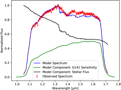
The reference coordinates $(X_{\textrm{ref}},Y_{\textrm{ref}})$ are determined by the photometric images taken at the beginning of each visit. Coefficients for converting this reference pixel to a reference wavelength (a₀, a₁) were determined empirically by Kuntschner et al. (2009, Table 5). The wavelength of light recorded by a particular pixel is dictated by the dispersion for the Y-coordinate of the reference pixel (Y${}_{\textrm{dispersion}}$) and the intrinsic offset (X${}_{\textrm{shift}}$, in pixels) between the location of the filter image and the grism-dispersed light. Y${}_{\textrm{dispersion}}$ and X${}_{\textrm{shift}}$ are constrained, but spatial scan mode complicates those values. Consequently, DEFLATE fits for these values by comparing an observed out-of-transit spectrum to an ATLAS stellar model (Castelli & Kurucz, 2004) convolved with the G141 grism sensitivity curve. The stellar model combines the line and continuum fluxes as ($\alpha\times$Line + Continuum), essentially allowing the strength of the stellar lines to vary to compensate for metallicity or other opacity mismatches. Figure 1 shows the result of the fit for L98-59 c.

Figure 1: The model we generated for the stellar spectrum provides a good match to the observed spectrum over the G141 wavelength range.

We determined the wavelength solution separately for both the forward-scan and reverse-scan light curves. The forward and reverse scans tend to be offset vertically from one another by a small amount, and the difference in wavelength solution is never more than 3% and typically around 1.5%, well within the size of a detector pixel (i.e, subpixel shift). We find that the wavelength solution is not significantly impacted by exact stellar model choice, or error scaling, or line-strength scaling.

DEFLATE uses the downloadable WFC3 flatfield files to divide out the flat-field from both the data and the error array (to propagate uncertainty), and removes the cal-wfc3-flagged “bad” pixels (which are identical across all exposures) by giving them zero-weight. It is possible to interpolate flux values at these pixels, but we prefer the zero-weight method since it requires fewer assumptions. The zero-weight pixels make up roughly 2% of all pixels in an exposure. DEFLATE also uses a corrected median time filter to flag cosmic rays. Before applying the filter, DEFLATE normalizes each pixel by the median of its row, which prevents DEFLATE from flagging entire rows as cosmic rays since they are distorted by time-dependent instrumental effects, inconsistent spatial scan rates, and obviously the transit/eclipse itself. We then use a double-sigma cut, first applying an 8$\sigma$ cut to remove any extreme outliers, then applying a second 5$\sigma$ cut to correct the remaining energetic particles. Less than 0.5% of all pixels in L 98-59 c’s observations are impacted by cosmic rays, and typically only a few pixels per exposure are impacted.

Finally, DEFLATE follows a simple procedure to define a light curve extraction aperture. It first defines the maximum flux of an exposure as the median of the five rows with the greatest flux. The edge of the box is set to the outermost row and column with a median value of greater than 3% of the maximum flux. This relatively low cut-off captures the entire first-order spectrum and minimizes the impact of vertical shifts. This method maximizes the SNR from the source and avoids over-processing the data.

3 Light Curve Analysis

Modeling a transit light curve has two major components: modeling the physical transit, and modeling the non-astrophysical instrumental effects related to how the WFC3 instrument collects flux, i.e. the instrumental systematics. WFC3 observations commonly exhibit several instrumental effects; the most prominent effects are a hook/ramp feature due to charge-trapping, a visit-long decrease in flux, a “breathing” effect based on changing temperatures during HST’s orbit, and a wavelength jitter effect (e.g, Berta et al., 2012; Wakeford et al., 2016; Zhou et al., 2017; Tsiaras et al., 2018, among many others). These features vary in magnitude across different observations in non-obvious ways. There is no encapsulating physically-motivated model to describe all of these effects (though recently individual features have been modeled more successfully, e.g. Zhou et al. (2017)). Instead of using inherent properties of the detector, these features are typically removed using empirical methods (Gibson, 2014a; Nikolov et al., 2014; Haynes et al., 2015). For this work, we use a new version of parametric marginalization, a Bayesian model averaging strategy that was conceptually introduced to exoplanet light curves by Gibson (2014b) and first applied to WFC3 transit spectroscopy by Wakeford et al. (2016).

3.1 Modeling the Light Curves

Similar to Wakeford et al. (2016), we find that fourth-order polynomial parameterizations consistently describe the systematic effects while preserving computational time. We use a grid of models that include up to four powers of HST phase, four orders of wavelength shift, and 5 forms of a orbital phase-dependent visit-long slope (none, linear, quadratic, exponential, and log). Each higher power includes all lower powers (e.g, 3rd order HST phase is a${}_{0}\times$HST + a${}_{1}\times$HST² + a${}_{2}\times$HST³), and there are no cross terms. This results in a grid of 125 systematic models (5 possible HST powers $\times$ 5 possible shift powers $\times$ 5 possible slope parameterizations). There are an additional two parameters: separate normalization constants for the forward (A_f) and reverse scans (A_r). It is typical for the two directions to be offset, though that is the primary effect and they can still be fit simultaneously.

It is computationally difficult to efficiently sample the parameter space of all 125 models using Markov Chain Monte Carlo (MCMC) samplers, so we instead fit each model using KMPFIT (Terlouw & Vogelaar, 2015), a Python implementation of the Levenberg-Markwardt least squares minimization algorithm, to quickly determine parameter values and uncertainties. Wakeford et al. (2016) found that uncertainties derived from these two methods typically agree within 10%; we also find excellent agreement, and that KMPFIT (for a single model) tends to overestimate uncertainty relative to MCMC. We then weight each model by its Bayesian evidence — approximated by the Akaike information criterion (Akaike, 1974) — and marginalize over the model grid (assuming a prior that each model is equally likely) to derive the light curve parameters and uncertainties while inherently accounting for uncertainty in model choice.

Figure 2: Visualization of white light curve fit for the highest weighted systematic model for L 98-59 c demonstrate a good model fit to the observed data. Panel (a) shows the band-integrated light curve. Panel (b) shows the de-trended light curve as well as the best fitting transit model. Note that this is illustrative – the instrumental effects and transit model parameters are fit for simultaneously. Panel (c) shows the residuals between the data and the best-fitting model.

Figure 3: Corner plot of astrophysical parameters for MCMC fit of highest weighted systematic model. The model converged and derived uncertainties slightly less than KMPFIT’s.

DEFLATE uses BATMAN transit models (Kreidberg, 2015) for the physical component of the light curve model. The model strongly constrains the transit depth (R_p/R_s) and center of transit time (T₀) with weak constraints on scaled semi-major axis (a/R_s), inclination (i), and a linear limb-darkening coefficient (c₀). We assume nonlinear limb darkening (LD) and derive the coefficients by interpolating values from Claret et al. (2012) to the central wavelength of WFC3 (1.4 $\mu$m). These coefficients are fixed for light curve fitting as HST’s poor phase coverage does not well constrain the shape of transit. We also compared with LD values from earlier models by Claret & Bloemen (2011) to be sure results are not sensitive to LD source and tested a linear LD law with the coefficient being a fittable parameter.

3.2 White light modeling

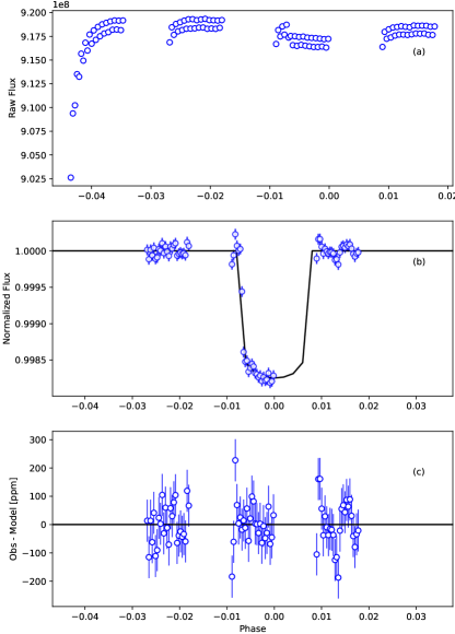
We first fit the white light curves, which provided a confidence check on the data, maximizes SNR for deriving wavelength-independent properties such as inclination and a/R_s, and captured the structure of residuals for each systematic model, if present. Determining the residuals allowed us to further de-trending of spectral curves via white light residual removal (Mandell et al., 2013; Haynes et al., 2015). While this method is suitable for M-dwarf targets that near constant flux across the bandpass, we caution that this method is not generally applicable to hotter stars. We fixed the orbital period, inclination, and $a/R_{s}$ to their values in Table 1, and only allow linear visit-long slopes, since the L 98-59 dataset only has three usable orbits covering a small amount of the out-of-transit baseline. As is common practice, we ignore the systematic-dominated first orbit in the white light analysis; however, the use of common-mode detrending provides the option of including that orbit in the spectral light curve analysis. The raw light curve, the light curve with instrumental systematics removed, and the residuals from the highest-weight systematic model are shown in Figure 2. The derived transit depths and center-of-transit times (T_c) are given in Table 2. We measured the white light depth to be $1620\pm{24}$ ppm. The derived depths are insensitive to model assumptions, varying no more than 20 ppm when linear LD was fit for, or if $a/R_{s}$ was fit for, or if a quadratic visit-long slope was assumed. The reduced chi-squared of each fit was around 1.2, which is typical of HST white light curves.

Table 2: L 98-59 c White light Curve-measured Transit Parameters

Observation	Transit Depth	Tc
	[ppm, $(R_{p}/R_{s})^{2}$]	[BJD-2457000]
L 98-59 c	$1620\pm{24}$	$1946.7068\pm{0.0001}$

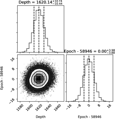
To further validate these results, and to make sure the derived uncertainties are reasonable, we fit the highest-weighted systematic model of L 98-59 c with MCMC (emcee; Foreman-Mackey et al., 2013). We also show the corner plot (Foreman-Mackey, 2016) of astrophysical parameters in Figure 3. The posterior of the transit depth is Gaussian. The two methods are in excellent agreement, down to the ppm: both find a depth of 1620ppm and the MCMC uncertainty is 98% of the KMPFIT uncertainty, with a posterior Gaussian distribution.

Figure 4: Spectral light curves for L 98-59 c, collected during the first visit.

3.3 Transit Spectra Derivation

Table 3: Transmission Spectra of L 98-59 c, with bin size 0.0279$\mu$m and resolution $\sim 50$

$\lambda$ [$\mu$m]	Depth [ppm]
1.123–1.151	1561 $\pm$ 56
1.151–1.179	1609 $\pm$ 55
1.179–1.207	1686 $\pm$ 54
1.207–1.235	1600 $\pm$ 52
1.235–1.263	1616 $\pm$ 51
1.263–1.291	1539 $\pm$ 59
1.291–1.318	1585 $\pm$ 49
1.318–1.346	1572 $\pm$ 51
1.346–1.374	1658 $\pm$ 53
1.374–1.402	1628 $\pm$ 56
1.402–1.430	1693 $\pm$ 56
1.430–1.458	1697 $\pm$ 55
1.458–1.485	1721 $\pm$ 53
1.485–1.513	1665 $\pm$ 52
1.513–1.541	1549 $\pm$ 54
1.541–1.569	1662 $\pm$ 54
1.569–1.597	1625 $\pm$ 54
1.597–1.625	1739 $\pm$ 55
1.625–1.653	1635 $\pm$ 54

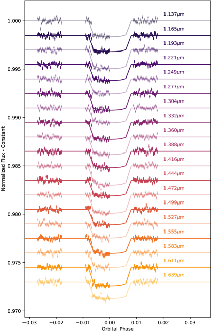
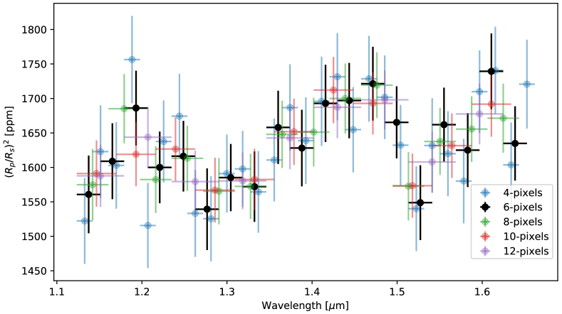
To derive the transit spectrum, we binned the 1-D spectra from each exposure between the steep edges of the grism response curve (1.1–1.6 $\mu$m), deriving a flux time-series for each spectral bin. We tested several bin widths since the long scan observations (close to 300 rows) are more at risk of wavelength blending (Tsiaras et al., 2016), which will effect larger bins less than smaller ones. We find no difference as a function of bin width (see Figure 5), and we choose 6-pixel-wide (0.0279 $\mu$m) bins to maximize resolution without drowning the signal in noise. The spectrum is given in Table 3, and the spectral light curves are shown in Figure 4.

Figure 5: The marginalization-derived transit spectrum for L 98-59 c at different resolutions all show evidence for a non-flat spectrum. The shape of the spectrum is not sensitive to the spectral bin size.

3.3.1 WFC3 Transit Spectrum Verification

Marginalization is only reliable if at least one model is a good representation of the data (Gibson, 2014b; Wakeford et al., 2016). We therefore checked the goodness-of-fit of the highest-weighted systematic model for each light curve using both reduced $\chi^{2}$ and residual normality tests. We further explored if red noise is present in the light curve residuals, as that can bias inferred depth accuracy and precision (Cubillos et al., 2017).

Though $\chi^{2}$ cannot prove that a model is correct, it can demonstrate that the fit of a particular model is not inconsistent with the observed data (Andrae et al., 2010). Therefore it is an informative goodness-of-fit diagnostic, and it is particularly useful due to its familiarity and simplicity. An ideal fit would have a reduced $\chi^{2}$ of one with uncertainty defined by the $\chi^{2}$ distribution. For both the band-integrated and spectral light curves ($\sim 60$ degrees of freedom), this resulted in an reasonable reduced $\chi^{2}$ range of roughly 0.66–1.4.

Figure 6: Binned RMS analysis for each spectral bin (see Section 3.3.1). The RMS of the data residuals are shown by the colored lines. The solid black line is the theoretical trend from Cubillos et al. (2017). The dashed-white line is the median value from simulated pure white noise residuals. The gray regions are the 1- and 2-$\sigma$ ranges for the simulated white noise residuals, which demonstate that the observed data is consistent with largely uncorrelated noise.

Figure 7: The blue lines and dots show the autocorrelation function (as a function of lag) for each spectral bin, with lag 0 left out for clarity. The solid red lines indicate the 2$\sigma$ range: autocorrelation value within these lines are not considered significant. The observed data has minimal significant autocorrelation.

The band-integrated analysis ($\chi^{2}_{\nu}=1.2$) and all spectral bins (median $\chi^{2}_{\nu}=0.9$) fall within the expected range. The exception is the 1.499 $\mu$m light curve, whose highest-weighted model fit has a reduced $\chi^{2}$ of 0.59. This low value indicates that the uncertainties in this light curve are probably overestimated. This is likely due to incorporating white light residuals, which both inflate uncertainties and can potentially interpret random white noise as structure. However, it is not flagged by the normality or correlated noise analyses (described below), and fitting the light curve without incorporating white light residuals finds a consistent depth with a more reasonable $\chi^{2}_{\nu}=0.9$; we therefore include it in the transit spectrum. For the other spectral bins, the reduced $\chi^{2}$ values provide no evidence against validity of the derived transit depths and uncertainties.

A residual normality test checks if the residuals for a model are Gaussian-distributed to determine goodness-of-fit, since this would be expected a model that well describes the data provided the errors are Gaussian distributed. Like reduced $\chi^{2}$, a normality test cannot prove that a model is correct, but can only diagnose incorrect models. We use the scipy implementation of the common Shapiro-Wilk test for normality (Shapiro & Wilk, 1965), and determine for which light curves the highest evidence model has normality ruled out at the $5\%$ significance level. At a sample size of around 75 this is by no means rigorous, but it is still a useful heuristic for flagging potentially problematic light curve models. Normality is rejected at the $5\%$ significance level only for the 1.14 $\mu$m spectral bin residuals; however, it is ruled out due to a single outlier in the time-series. When this exposure was ignored, we recovered a consistent depth and uncertainty and the residuals are consistent with normality. Further, ignoring residuals again recovered almost the exact same depth without any normality flags. We therefore kept this exposure in the analysis.

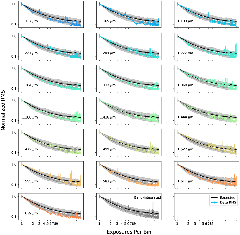
Finally, we tested for correlated noise in the residuals following the time-average methodology of Cubillos et al. (2017) (also see Pont et al. (2006)) and using MC³. Noise can be thought of as the sum of a purely white (random) noise and a time-correlated (red) noise: $\sigma_{total}=\sqrt{(}\sigma^{2}_{w}/N+\sigma^{2}_{r})$ (Pont et al., 2006). As randomly distributed residuals with mean of zero (i.e, if uncorrelated white noise is the dominant uncertainty source) are averaged in time, the scatter in the points decreases proportional to $\sigma_{w}/\sqrt{N}$. If red noise is significant, then the time averaging only decreases noise until it flattens out at $\sigma_{r}$. One can test for the impact of red noise by time-averaging the residuals and comparing the resulting RMS function to theoretical expectations of white noise. Though this method is not necessarily rigorous for HST due to the relatively small number of exposures, it is still a practical diagnostic. We improved upon this method by simulating synthetic normally-distributed residuals with the same standard deviation as the actual residuals, and putting them through the same method (Figures 6 and  7). We note the 1 and 2$\sigma$ bands for random, pure white noise residuals compared to the results for the actual residuals. For every bin, the residuals are consistent with random white noise for every bin size. We find no evidence of correlated noise.

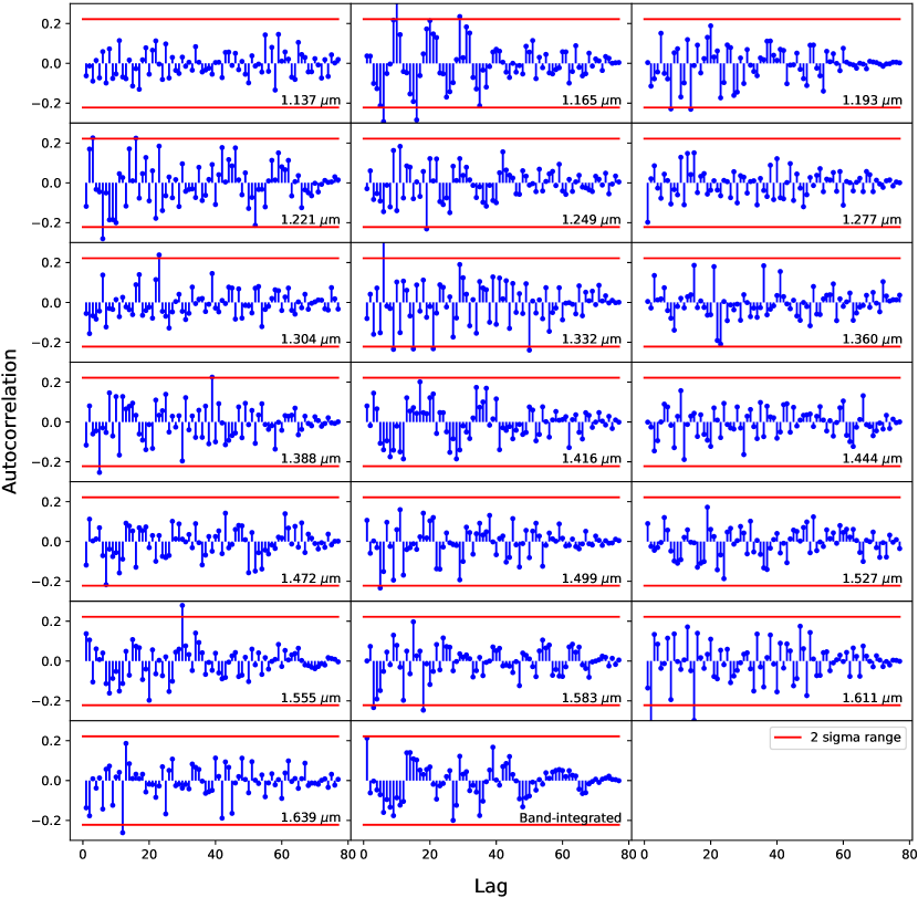
We also visualized correlated noise by looking at the autocorrelation function of the residuals. This method is not purely quantitative, but can provide another look at potential structure in the residuals. The red lines in Figure 7 indicate the 2$\sigma$ line – roughly indicating “significant” correlations at that lag. Note that a few lags passing this line is not problematic, since 2-sigma events happen roughly 5% of the time and we are sampling many bins. This is less quantitative, but autocorrelation functions that appear too structured can be, unsurprisingly, indicative of structured noise. An example might be 1.165 $\mu$m, which appears to be a decreasing sinusoid; however, structure below significance is less problematic. Different derivation assumptions give the same transit depth at this bin without structured residuals, and it passes the other red noise test, so we have confidence in the depth determination.

With the caveats noted above, marginalization does an excellent job in fitting the spectral light curves. Together, these tests support the validity of the derived transit depths and uncertainties.

4 Exploratory Analysis of Potential Atmospheres with PLATON

In the subsequent sections, we study whether the apparent structures in the spectra of L 98-59 c are significant and indicative of an atmosphere with a reasonable chemical composition. Only a low mean-molecular weight atmosphere could produce spectral features with amplitudes similar to the features seen in our results (roughly 100 ppm) (Kreidberg, 2018). However, due to the relatively large error bars on each individual spectral bin, it is not obvious that a model with molecular features would be a significantly improved fit over a straight line (indicative of no atmosphere or high-altitude clouds). Further, stellar activity can potentially contaminate transit spectra and mimic molecular features (Barclay et al., 2021).

We utilized two different strategies to investigate the potential for detecting an atmosphere. We first used the open-source retrieval tool PLATON (Zhang et al., 2019) to perform a Bayesian statistical retrieval of the atmospheric parameters assuming a H₂-rich composition and equilibrium chemistry. We then examined the ability to constrain the presence of individual molecular constituents using a more simplistic fitting scheme for combinations of individual absorbers with the Planetary Spectrum Generator (PSG, Villanueva et al., 2018).

4.1 PLATON Atmospheric Modeling and Retrieval Methodology

PLATON is open-source retrieval software developed by Zhang et al. (2019), which comprises a forward model and an algorithm for Bayesian inference. Though there are minor differences, it essentially uses the same forward model as Exo-Transmit (Kempton et al., 2017). The software assumes an H₂-He/dominated atmosphere, and though it has recently incorporated free retrieval capabilities, in this study we exclusively used the version which assumes chemical equilibrium. Though these constraints naturally limit the types of planetary atmospheres that can be explored, it was useful in contextualizing the spectrum and investigating the likelihood of an H₂-dominated atmosphere on L 98-59 c.

Table 4 describes the parameters and their priors for the PLATON atmospheric retrieval. We allowed planet radius, C/O, metallicity, temperature, and cloudtop pressure to vary, and assumed an isothermal temperature profile. C/O and metallicity dictate the elemental ratios in the atmosphere, which are input with temperature into a chemical equilibrium code (ggchem; Woitke et al., 2018) to determine the abundance of every species at every pressure layer. Each chemical parameter was given a prior set by computational limits (most notably T_min=300 K), and the mass/radius priors were set by literature values (Demangeon et al., 2021); we included stellar radius and planetary mass in order to propagate the literature uncertainties forward. The retrieval utilized nested sampling (Skilling, 2004; Speagle, 2020) with 200 live points to sample the parameter space and calculate a Bayesian evidence for the model. The assumed C/O ratio is the Solar value.

Table 4: Priors for parameters used in L 98-59 c Retrievals

Parameter	Symbol	Prior Dist.
Planet Radius [$R_{\oplus}$]	$R_{p}$	$\mathcal{U}(0.7,2.1)$
Limb Temperature [K]	$T$	$\mathcal{U}(300,1100)$
Carbon-oxygen ratio	C/O	$\mathcal{U}(0.05,2.0)$
Metallicity	$Z$	$\mathcal{LU}(-1,3)$
Planet Mass [$M_{\textrm{Earth}}$]	$M_{p}$	$\mathcal{N}(2.22,0.26)$
Stellar Radius [$R_{\odot}$]	$R_{s}$	$\mathcal{N}(0.30,0.02)$
Cloudtop Pressure [Pa]	$P_{\textrm{cloud}}$	$\mathcal{LU}(-3,8)$
Stellar Effective Temperature [K]	$T_{\textrm{star}}$	Fixed
Spot Temperature [K]	$T_{\textrm{spot}}$	Fixed
Spot covering fraction	$f_{\textrm{spot}}$	$\mathcal{U}(0,0.5)$

4.2 PLATON Retrieval Results

The retrieval finds a best model fit with $\chi^{2}_{\textrm{Red}}$ = 1.15. The resulting posterior distributions and best-fit model spectra from the retrieval are shown in Figure 8. Under the assumption that L 98-59 c has a H₂-dominated atmosphere with no disequilibrium processes L 98-59 c was best described as a high-metallicity atmosphere (Z$\sim 250\times$Z_⊕) with a likely super-solar C/O ratio. The retrieved atmospheric metallicity was consistent with predictions from the hypothesized mass-metallicity relationship from the Solar System planets (e.g, Fortney et al., 2013), and the retrieved R_p was consistent with the literature (1.30$\pm$0.07 R_⊕). The atmospheric temperature was poorly constrained, which is expected for a retrieval of transmission spectrum, and the cloud-top pressure was also weakly constrained due to the narrow wavelength coverage and the large uncertainties on the data. The best-fit model yielded small water features at 1.4 $\mu$m and 1.1 $\mu$m, but there was no statistically significant water detection. We note that the inferred water feature at 1.4 $\mu$m is roughly 100 ppm, which is consistent with predictions of the feature size for a H₂-dominated atmosphere (assuming 4 scale heights; derived from Kreidberg (2018)).

PLATON also allows for model comparison, since nested sampling naturally calculates the Bayesian evidence of a model. Although this evidence cannot act as an absolute goodness-of-fit metric, the ratio of two evidences provides a straightforward measure of how much more likely one model is in comparison to the other. This ratio is known as the odds ratio ($\mathcal{O}_{12}=\mathcal{Z}_{1}/\mathcal{Z}_{2}$), and is directly interpreted as “Model 1 is $\mathcal{O}_{12}\times$ more probable than Model 2”. There are also empirically-determined benchmarks for converting $\mathcal{O}$ into more familiar $\sigma$-level significance (Trotta, 2008; Benneke & Seager, 2013).

Figure 8: Retrieval results for L 98-59 c. Left: Corner plot for the best-fit fiducial H₂-dominated atmosphere. Upper right: Best fit assuming a flat spectrum (high clouds or no detectable atmospheric features). Lower right: Model spectrum assuming the median retrieved parameter values (green triangles) with 1 and 2-sigma contours (red) plotted over data (blue).

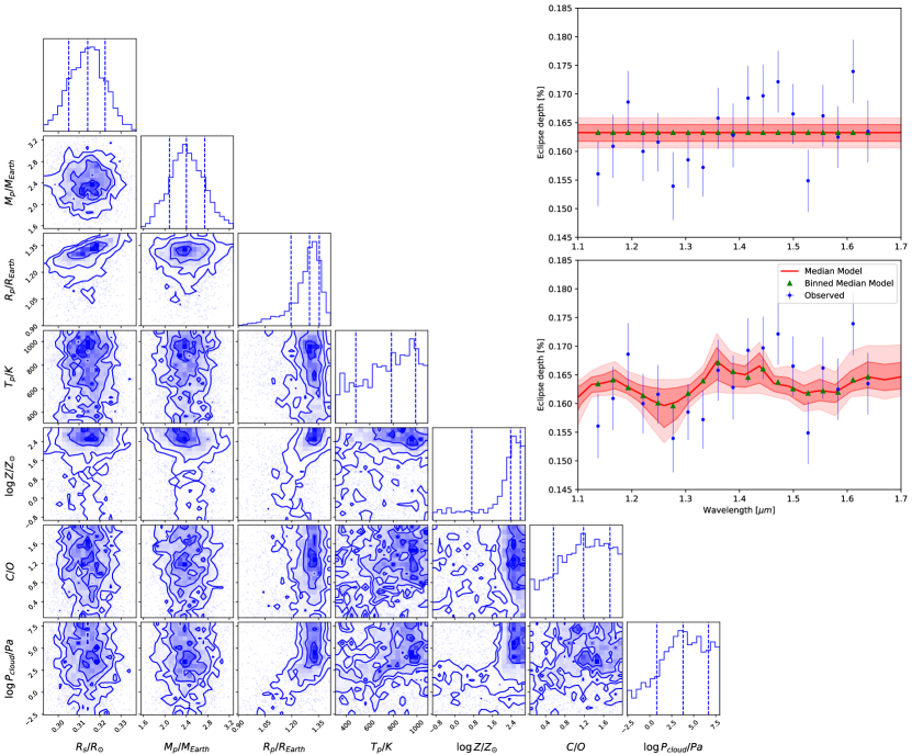
To determine the likelihood of an H₂ atmosphere on L 98-59 c, we compared the evidence of the retrieved fiducial atmosphere to that of a flat line spectrum. We introduced a flat spectrum into PLATON by fixing a very high, grey cloud. We then only allowed planet radius to vary in the fit. The resulting fit is shown in the upper-right panel of Figure 8. The odds ratio between the fiducial model and the flat-spectrum model was 3, which corresponds to a “weak” detection of roughly 2.1$\sigma$, or about 75% probability. We note that the specific sigma significance is relatively imprecise, since even a small numerical error in $\mathcal{Z}$ – which is common (Speagle, 2020) – could shift the odds ratio slightly below the empirical cut-off. We also compare the Bayesian evidences between the fiducial atmosphere and the same atmospheric model with no water opacity, finding the odds ratio to be $\sim$1. This indicates that there is no conclusive evidence of the presence of water vapor in the atmosphere. The evidence of water vapor specifically is weaker than that of the full atmosphere model since other opacity sources (e.g, NH₃) can “fill in” for water vapor and capture some of the structure in the observed spectrum.

5 PSG Atmospheric Modeling and Retrieval

The PLATON forward model and retrieval framework includes a number of assumptions about the atmospheric composition and structure that limit the ability to examine the evidence for individual atmospheric absorbers. For these reasons we also opted for an exploratory model-fitting approach using the Planetary Spectrum Generator (PSG), in which we analyze the potential for a molecular detection by looking at how well simulated spectra with a number of potential atmospheric absorbers fit the data. To quantify the goodness of the fit we used the reduced $\chi^{2}$ of the data and the model, and we examined the $\chi^{2}$ across a range of molecular combinations and abundances.

PSG (Villanueva et al., 2018, 2022) is a radiative transfer model and tool for synthesizing/retrieving planetary spectra (atmospheres and surfaces) for a broad range of wavelengths (50 nm to 100 mm, UV/Vis/near-IR/IR/far-IR/THz/sub-mm/Radio) and includes instrument/retrieval methods for a large variety instruments and observatories. As part of the retrieval framework of PSG, the tool has access to a Nested Sampling algorithm and an Optimal Estimation algorithm (Rodgers, 2000) to analyze planetary data and retrieve atmospheric/surface/physical parameters of interest via minimization of spectral residuals.

Simulated spectra with PSG include molecular, atomic, aerosol and continuum (e.g., Rayleigh, Raman, CIAs) radiative and scattering processes, which are implemented via a layer-by-layer framework. Many spectral databases are available in PSG, but for this study we have employed the molecular parameters from the latest HITRAN-2020 database (Gordon et al., 2022) that is implemented using a correlated-k method. This molecular database is complemented in the UV/optical with cross-sections from the Max Planck Institute of Chemistry database (Keller-Rudek et al., 2013). Besides the collision-induced absorption (CIA) bands available in the HITRAN database, the MT_CKD water continuum is characterized as H₂O–H₂O and H₂O–N₂ CIAs (Kofman & Villanueva, 2021).

For this simulation we omitted aerosols, clouds, haze, etc. and removed all molecules other than the two we wished to explore for any given simulation. The structure of the atmosphere was described in PSG by specifying for each layer the pressure (bars), temperature (K), and the abundances of atmospheric constituents with respect to the total gas content. For each gas, layer-by-layer integrated column densities (molecules m^-2) were then computed along the transit slant paths employing a pseudo-spherical and refractive geometry. We assumed the molecule abundance did not vary with temperature nor pressure, but rather was held consistent throughout the atmosphere. However, pressure and temperature were varied throughout the atmosphere using the Parmentier & Guillot (2014) model.

5.1 Chi-Squared Analysis Methodology

As previously pointed out, the large error affecting each spectral bin may be too large to clearly discern the abundance of gaseous species of interest by working with a classical retrieval approach, in which one tries to constrain abundance and uncertainty simultaneously for a set of species. Besides this, the spectral resolution is low enough that it would be challenging to uniquely distinguish molecular signatures from the spectral continuum.

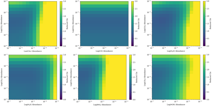
To estimate the presence of each molecule, we evaluate the reduced $\chi^{2}$ of specific models. Each model is produced by fixing the abundance of two gases of interest to two values, chosen in a given range. Then, the retrieval tool of the PSG is used to retrieve the planetary radius as the only free parameter, as that can be reliably constrained by the average intensity of the observed spectral continuum (as seen in Figure 8). For each fit, we retrieved only for diameter, while exploring the molecules by varying the pair abundances at each retrieval. We stored the reduced $\chi^{2}$ from the fit, and produced two-dimensional views of the reduced $\chi^{2}$ for each combination of gases and their respective abundances. This procedure is repeated for several combinations of gases, yielding a comprehensive view of the likelihood that the presence of those specific gases in the atmosphere may well fit the observed spectrum.

In this sense, the result of this approach is similar to what is commonly done by statistically sampling the parameter space via nesting or Monte-Carlo approaches. In this case, we explored the parameter space to locate a region where the reduced $\chi^{2}$ has a minimum. Those gases characterized by a clear minimum in the reduced $\chi^{2}$ in correspondence of a specific concentration are those that are more likely to be present in the atmosphere. Vice-versa, those who do not yield a clear reduced $\chi^{2}$ minimum for any concentration are likely not to be detectable above the noise level.

5.2 Results of the PSG model

The molecules were explored with abundances ranging from 10^-7 to 10^-2 volume mixing ratio. CO₂ was assumed to be present in each simulation, while the second molecule varied between five others: CH₄, H₂O, H₂S, NH₃, and HCN. We chose to include any molecular species that was present at abundance greater than 1 ppb and had absorption lines within 200 to 1000 nm, as trace secondary molecules. We also assumed an H₂ rich atmosphere, as the combination of an H₂ rich atmosphere, trace molecules, and no clouds is the most consistent with the observations.

As can be seen in Figure 9, the lowest reduced $\chi^{2}$ values (between 0.5 and 1.0) can be found at approximately 10^-4 VMR, or 10² ppm, CO₂ abundance. For each of the other trace molecules, this minima is achieved at extremely low abundances, 10^-6 or lower. While we searched for CO, its high-energy, low-intensity bands in this wavelength range, led to no fit improvement or detriment, thus it was not included in further analysis.

Figure 9: The heat maps above portray the results of a two molecule atmosphere analysis. All of the presented analyses have the molecule CO₂ on the y-axis. In the top left we have CH₄, in the top middle we have CO, in the top right we have H₂O, in the bottom left we have H₂S, in the bottom middle we have NH₃, and in the bottom right we have HCN. All molecules have been presented in the volume mixing ratio. We retrieved for diameter at each abundance level, and calculated the reduced $\chi^{2}$ to find the best fit retrieval for diameter.

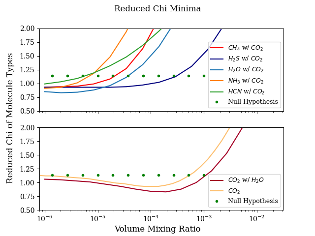
To expand on the results found in Figure 9, Figure 10 examines the direct molecular reduced $\chi^{2}$ when different molecules are locked to a value. In the top panel of the figure, all CO₂ concentrations are locked at 10^-4 VMR (i.e. the best fit value for CO₂), and the other molecules are free across the entire VMR range of 10^-7 to 10^-2. We also plotted the fit wherein we assume there is no atmosphere present, which presents a reduced $\chi^{2}$ of 1.14. As can be seen, the HCN and NH₃ lines cross the flat spectrum line just before 10^-5 VMR, and from that point forward make the fit worse. The CH₄ line crosses just after 10^-5. These molecules, if present, have extremely low abundances. This leaves the H₂O and H₂S lines, which cross the line for a flat spectrum at just before and after 10^-4 respectively. We extracted these molecular combinations that present the best reduced $\chi^{2}$ values, lock the trace molecules to their respective best values, and studied them further. In the lower panel, H₂O is locked at 10^-6 VMR and we examine the scenario wherein CO₂ is the only atmospheric molecule present. When the CO₂ and H₂S combination was examined, it was seen to be almost precisely the same as the CO₂ lines, and thus was omitted to prevent redundancy. Looking further at the lower panel of the plot, the CO₂ and H₂O combination results in the lowest reduced $\chi^{2}$ value reached in our simulation, approximately 0.83. Comparatively, the CO₂ simulation reached a reduced $\chi^{2}$ minima at 0.93. Both models cross the flat spectrum line just before 10^-3, at which point both models become less plausible than the potential of no atmosphere.

Figure 10: The reduced $\chi^{2}$ when various molecules are locked to their best-fit value. In the top panel, all CO₂ values are locked at approximately 10^-4 VMR while the other molecules are free. In the lower panel, H₂O is locked at approximately 10^-6 VMR. The value obtained with a flat transmission spectrum is presented in both panels as a dotted line, portraying the scenario in which there is no atmosphere present. This plot presents at which point every combination of molecules becomes a worse assumption than having no atmosphere - i.e. becoming an unrealistic scenario.

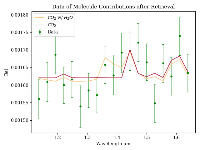
Shown in Figure 11 are the retrievals from the two best models described above in comparison to the L98-59 c data, with uncertainties. Figure 11 shows that our models well describe the observed data.The presence of H₂O is necessary for the model to fit the 1.35 to 1.5 $\mu$m wavelength region.

Figure 11: The plot above displays the best retrieval results from Figure 10, presented in the bottom panel. These retrieval results are presented with the actual data and error bars, to better portray the extent to which the model lies within the error bars.

6 Discussion

Herein, we presented HST observations of a single transit of the planet L98-59 c. Using data from the G141 grism setting for the WFC3 instrument on HST, we extracted a spectrum using our DEFLATE data reduction and analysis software. The final spectrum shows hints of deviations from a featureless spectrum, but the uncertainties on the data are sufficiently large to be fully consistent with a flat featureless spectrum (reduced $\chi^{2}=1.14$).

We performed atmospheric modeling with two different parameterized modeling schemes, using the open source tools PLATON (Zhang et al., 2019) and the Planetary Spectrum Generator (PSG, Villanueva et al., 2018), to determine limits on composition and cloud-top pressure that would still be consistent with the data.

The current uncertainties on the data are too large to conclusively determine anything beyond upper limits for a cloud-free or a deep-cloud scenario. However, our analysis with the PLATON Bayesian retrieval code as well as a $\chi^{2}$ analysis using forward models from PSG are both suggestive of molecular features. The PLATON retrieval finds a best-fit result consistent with a H2-dominated atmosphere with an elevated metallicity, while the PSG analysis finds that the data is best fit with with small contributions from H₂O and CO₂, with VMRs of 5$\times 10^{-6}$ and 9$\times 10^{-3}$ respectively.

6.1 Stellar Activity

L 98-59 was previously assumed to be a quiet star based on the analysis of TESS light curves. However, significantly more TESS data exists now than did when the planets were first identified (Kostov et al., 2019). We reexamined the TESS 2-minute cadence data, looking for signs of activity. We visually inspected approximately 14 months of TESS time-series data and saw five flares in the data, of which at least one shows a complex shape with two peaks. The flares are shown in Figure 12.

Figure 12: Five flares of L 98-59 seen in TESS 2-minute cadence data. The flares vary in peak fractional change in stellar brightness from 0.2% to 3.5%. There is also one complex flare that shows multiple peaks. The green curves are flare models with uncertainty regions inferred using an MCMC method.

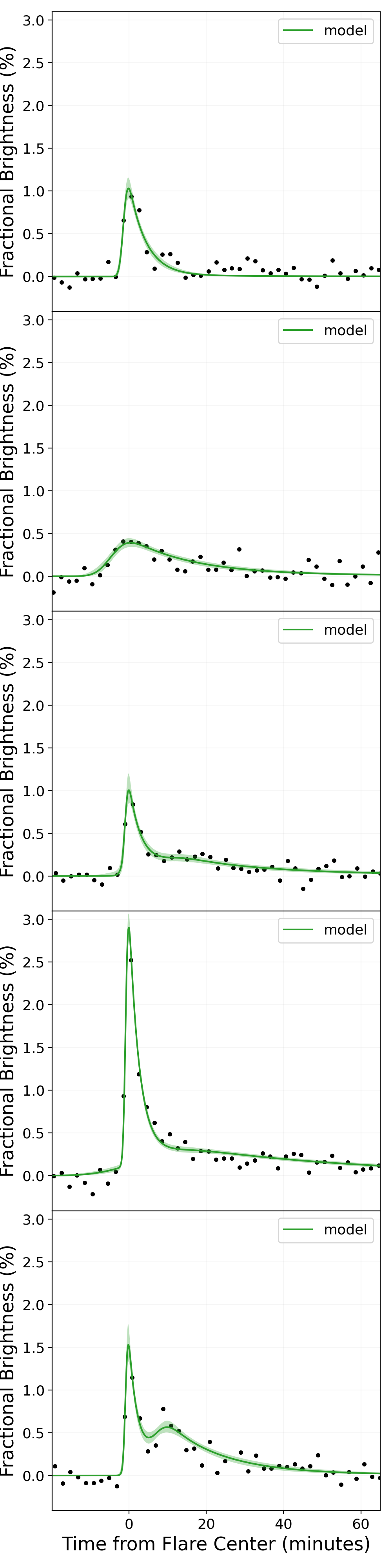
We modeled these five flares using software we developed called xoflares (Barclay & Gilbert, 2020). This version of the software implements the Mendoza et al. (2022) flare template. We sub-sampled the light curves by a factor of 7 to account for the non-linear changes in brightness occurring during a flare. The software uses Hamiltonian Monte Carlo method to efficiently sample the flare properties. We found that peak flare brightness ranged from 0.2% to 3.5%, which are not untypical values for mid-M dwarf stars (Paudel et al., 2021).

No rotational variability is visible in TESS data but with a rotational period of approximately 80 days (Demangeon et al., 2021) low amplitude variability would be challenging to measure. Given the activity identified, it is likely that L 98-59 has some level of surface inhomogeneities that could imprint into an exoplanet transmission spectrum (Rackham et al., 2018) because flares are frequently associated with starspots (Doyle et al., 2019). We performed an analysis similar to that presented in Barclay et al. (2021) to determine whether we could generate a model of contamination that could mimic the transmission spectrum seen in Figure 5. We were not successful – the fairly simple model used in the analysis of K2-18 b was not able to reproduce the shape of the peak around 1.45 $\mu$m that we see in the data. We could generate a peak at that location but this was always associated with a second broad peak near 1.3 $\mu$m. Moreover, generating a model that has a $>$100 ppm peak in the WFC3 G141 wavelenth range that also had no clear rotational modulation in TESS data was not possible. However, the analysis performed has numerous limitations. We are cautious in saying anything definitive on the possibility that stellar surface inhomogeneities could be corrupting the observed transmission spectrum because of our poor understanding of M-dwarf surfaces and the distribution of the parameters such as spot coverage, size distribution and spectral energy distributions.

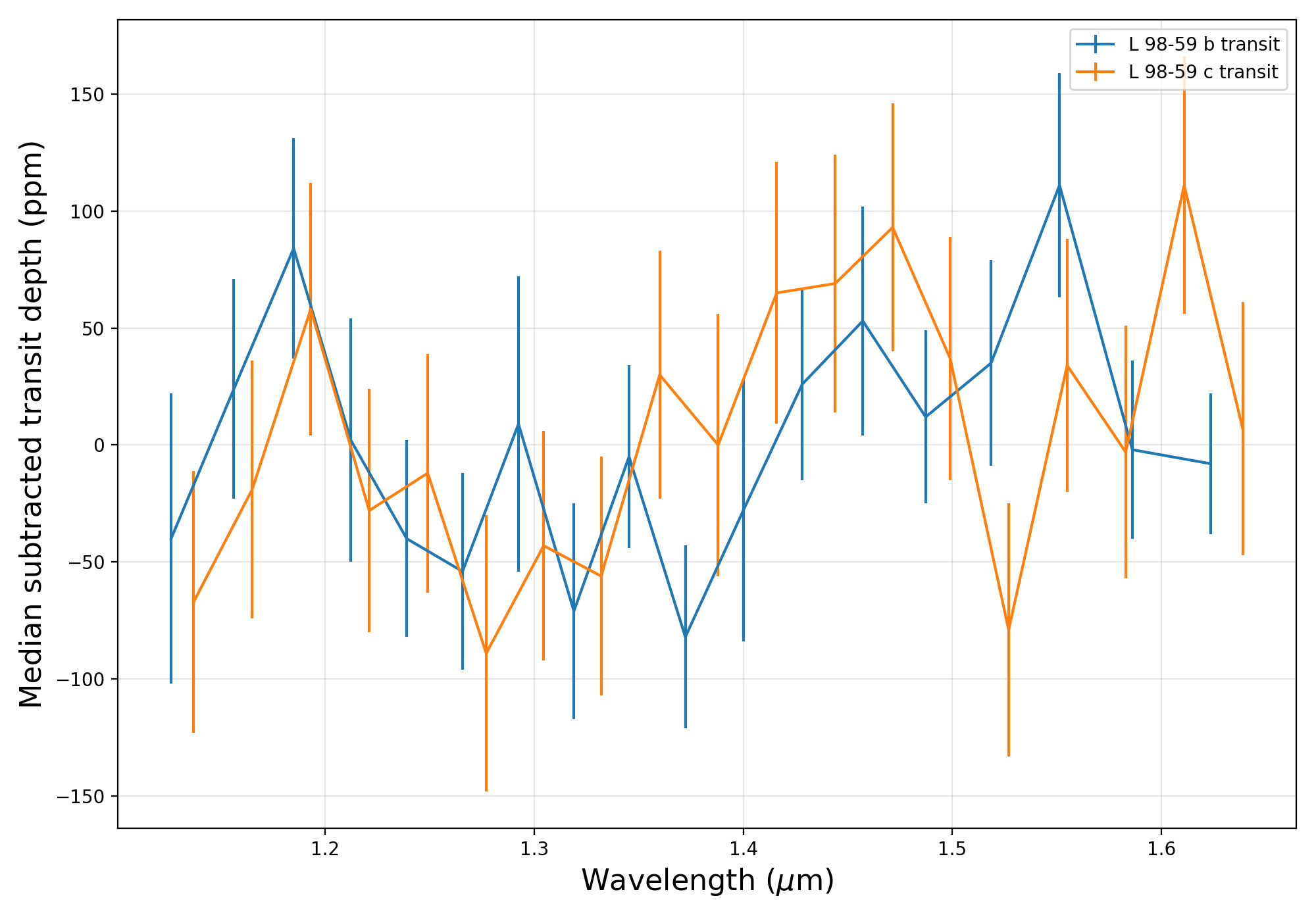
We also examined the HST observed transit of L 98-59 b collected on 2020-04-07, just 12.5 hours before the transit we are examining here. Our purpose in looking at these data was that if the L 98-59 c transit shows evidence for contamination, then is transit of planet b is likely to exhibit similar contamination signatures. This transit was the second of five observed for planet b, and showed properties largely consistent with the other four transits. However, using data from Damiano et al. (2022), the standard deviation of the Visit 2 transmission spectra data was the highest of all five visits, and the transit depth measured was also the lowest of all the observed transits, albeit at only a significance of $<$2$\sigma$. Additionally, in the wavelength range between 1.2–1.4 $\mu$m the values computed for Visit 2 is either the lowest or second lowest for each bin. This results in the appearance of an absorption peak around 1.45 $\mu$m similar to that seen in the L 98-59 c transit. Figure 13 shows the two transmission spectra overlaid with the median subtracted from each. There are similarities in the shape of the two transmission spectra. Both spectra have dips between 1.2–1.4 $\mu$m and both have absorption peaks between 1.4–1.5 $\mu$m.

In an effort to quantify whether the Visit 2 data is more similar to our L 98-59 c transit than the other transits we calculated the Pearson correlation coefficient between the planet c data and all visits of the planet b data using the pearsonr function from scipy (Virtanen et al., 2020). Visit 2 was the most correlated with the planet c data with a probability that the correlation between the datasets occurred by chance of only 13%, while the next highest was Visit 3 at 47% chance of the correlation occurring by chance. This difference implies that the correlation seen in Visit 2 is 3.6x less likely to have occurred by random chance than the correlation seen for Visit 3. This is indicative of the Visit 2 data being significantly more correlated than any of the other visits. However, we are not in a position to say whether the correlation is owing to a common systematic between the two data sets or whether this is simply a coincidence.

Figure 13: Observations of L 98-59 b and c were taken by HST just 12.5 hours apart. There is correlation between the two observations which could indicate a common systematic. The L 98-59 b data were shown here are from Visit 2 of 5, and are there dataset most correlated with the HST observations of L 98-59 c.

6.2 Future observations with HST

The spectrum reported here provides tantalizing hints of a detection of an atmospheric detection. However, the single transit observed limits the conclusions we can draw. A reliable detection will require additional data. Fortunately, L98-59 c has been selected for additional observations with HST to observe two more transits. As the observations are close to the shot noise limit, any increase in SNR should scale approximately with the square root of the number of transits observed. Furthermore, observing additional transits provides a robustness against a false positive detection owing to stellar activity.

6.3 A System of Benchmark Planets

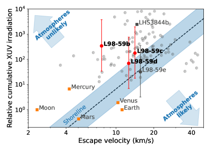
The L98-59 system provides an excellent opportunity to explore the atmospheres of small planets that evolved in the same stellar environment. The system also provides a unique opportunity to study the “Cosmic Shoreline” hypothesis (Zahnle & Catling, 2017), which suggests that there should be a relation between planetary mass and XUV irradiation that defines a boundary between planets with and without an atmosphere. Although L 98 59 has been previously observed by XMM-Newton, it is challenging to use these data to determine XUV flux because (a) it is missing the UV component, and (b) using single snapshots as a measurement for the integrated XUV flux is biased because flares can occur during observations. So while the integrated XUV history of L 98-59 is not well constrained, using the uncertainties of XUV fluxes representative of M-dwarfs (Shkolnik & Barman, 2014), planets c and d reside near the shoreline (Figure 14) (Kite & Barnett, 2020). If either planet is found to retain an atmosphere, we could place a constraint on the location of the shoreline; alternatively, if the planets are found to be inconsistent with the hypothesis, it would suggest other mass loss processes (such as impact erosion) are dominant (Kegerreis et al., 2020).

L 98-59 c and d are also both in the Venus Zone regime (Kane et al., 2014). Venus Zone planets are critical for comparative planetology efforts that aim to characterize the conditions for planetary habitability, and L98-59 could become a benchmark system for examining Venus-class planets that can help place our solar system into context.

Figure 14: The L98-59 system provides a unique opportunity to probe the cosmic shoreline. In the solar system, the light blue region separates bodies that have atmospheres from those that don’t (Zahnle & Catling, 2017). Grey dots show known rocky exoplanets with R$<$1.6 R_⊕ and measured masses and radii. The integrated XUV history of L98-59 is unknown, so the vertical error bars are representative of M-dwarfs (Shkolnik & Barman, 2014).

7 Conclusions

We observed a single transit of L 98-59 c with Hubble’s WFC3 and find some evidence that the transmission spectrum is not flat, indicative of an exoplanet atmosphere. However, the detection has low significance. While we are cautiously optimistic that our detection is real, our confidence is not high enough to make this a solid claim.

Since the original discovery of the L 98-59 planetary system, more TESS data has been obtained and the star is more active than previously thought. We were not able to simulate any scenarios where contamination could cause the detected signal, although more data will be useful as the spectra of stellar surface inhomogeneities is poorly constrained. We did find some suggestive anomalies about the transit of L 98-59 b collected just 12.5 hours prior to our L 98-59 c transit. This transit spectrum had the most scatter of any of the five collected, and in the region of wavelength-space where contamination is most problematic, this transit spectrum closely matched the shape of the L 98-59 c spectrum. This correlation is suggestive that both transits suffer from correlated systematics.

Fortunately, L98-59 c is scheduled to be observed by HST and JWST in the near future, which will likely resolve whether the signals we have detected are astrophysical in mature and caused by a planetary atmosphere.

References

- Akaike (1974) Akaike, H. 1974, IEEE Transactions on Automatic Control, 19, 716
- Andrae et al. (2010) Andrae, R., Schulze-Hartung, T., & Melchior, P. 2010, arXiv e-prints, arXiv:1012.3754. https://arxiv.org/abs/1012.3754
- Astropy Collaboration et al. (2013) Astropy Collaboration, Robitaille, T. P., Tollerud, E. J., et al. 2013, A&A, 558, A33, doi: 10.1051/0004-6361/201322068
- Astropy Collaboration et al. (2018) Astropy Collaboration, Price-Whelan, A. M., Sipőcz, B. M., et al. 2018, AJ, 156, 123, doi: 10.3847/1538-3881/aabc4f
- Barclay & Gilbert (2020) Barclay, T., & Gilbert, E. 2020, mrtommyb/xoflares, 0.2.1, Zenodo, doi: 10.5281/zenodo.4156285
- Barclay et al. (2021) Barclay, T., Kostov, V. B., Colón, K. D., et al. 2021, AJ, 162, 300, doi: 10.3847/1538-3881/ac2824
- Batalha et al. (2018) Batalha, N. E., Lewis, N. K., Line, M. R., Valenti, J., & Stevenson, K. 2018, ApJ, 856, L34, doi: 10.3847/2041-8213/aab896
- Batalha et al. (2023) Batalha, N. E., Wolfgang, A., Teske, J., et al. 2023, AJ, 165, 14, doi: 10.3847/1538-3881/ac9f45
- Benneke & Seager (2013) Benneke, B., & Seager, S. 2013, ApJ, 778, 153, doi: 10.1088/0004-637X/778/2/153
- Benneke et al. (2019) Benneke, B., Knutson, H. A., Lothringer, J., et al. 2019, Nature Astronomy, 3, 813, doi: 10.1038/s41550-019-0800-5
- Berta et al. (2012) Berta, Z. K., Charbonneau, D., Desert, J.-M., et al. 2012, The Astrophysical Journal, 747, 35, doi: 10.1088/0004-637X/747/1/35
- Bourrier et al. (2017) Bourrier, V., Ehrenreich, D., King, G., et al. 2017, A&A, 597, A26, doi: 10.1051/0004-6361/201629253
- Bourrier et al. (2018) Bourrier, V., Dumusque, X., Dorn, C., et al. 2018, A&A, 619, A1, doi: 10.1051/0004-6361/201833154
- Burt et al. (2021) Burt, J. A., Dragomir, D., Mollière, P., et al. 2021, AJ, 162, 87, doi: 10.3847/1538-3881/ac0432
- Castelli & Kurucz (2004) Castelli, F., & Kurucz, R. L. 2004, arXiv.org, 5087
- Claret & Bloemen (2011) Claret, A., & Bloemen, S. 2011, A&A, 529, A75, doi: 10.1051/0004-6361/201116451
- Claret et al. (2012) Claret, A., Hauschildt, P. H., & Witte, S. 2012, A&A, 546, A14, doi: 10.1051/0004-6361/201219849
- Cloutier et al. (2019) Cloutier, R., Astudillo-Defru, N., Bonfils, X., et al. 2019, A&A, 629, A111, doi: 10.1051/0004-6361/201935957
- Crossfield et al. (2020) Crossfield, I. J. M., Dragomir, D., Cowan, N. B., et al. 2020, ApJ, 903, L7, doi: 10.3847/2041-8213/abbc71
- Cubillos et al. (2017) Cubillos, P., Harrington, J., Loredo, T. J., et al. 2017, AJ, 153, 3, doi: 10.3847/1538-3881/153/1/3
- Damiano et al. (2022) Damiano, M., Hu, R., Barclay, T., et al. 2022, AJ, 164, 225, doi: 10.3847/1538-3881/ac9472
- de Wit et al. (2016) de Wit, J., Wakeford, H. R., Gillon, M., et al. 2016, Nature, 537, 69, doi: 10.1038/nature18641
- de Wit et al. (2018) de Wit, J., Wakeford, H. R., Lewis, N. K., et al. 2018, Nature Astronomy, 2, 214, doi: 10.1038/s41550-017-0374-z
- Demangeon et al. (2021) Demangeon, O. D. S., Zapatero Osorio, M. R., Alibert, Y., et al. 2021, A&A, 653, A41, doi: 10.1051/0004-6361/202140728
- Deming et al. (2013) Deming, D., Wilkins, A., McCullough, P., et al. 2013, ApJ, 774, 95, doi: 10.1088/0004-637X/774/2/95
- Diamond-Lowe et al. (2020) Diamond-Lowe, H., Berta-Thompson, Z., Charbonneau, D., Dittmann, J., & Kempton, E. M. R. 2020, AJ, 160, 27, doi: 10.3847/1538-3881/ab935f
- Diamond-Lowe et al. (2018) Diamond-Lowe, H., Berta-Thompson, Z., Charbonneau, D., & Kempton, E. M. R. 2018, AJ, 156, 42, doi: 10.3847/1538-3881/aac6dd
- Diamond-Lowe et al. (2022) Diamond-Lowe, H., Mendonca, J. M., Charbonneau, D., & Buchhave, L. A. 2022, arXiv e-prints, arXiv:2210.11809, doi: 10.48550/arXiv.2210.11809
- Doyle et al. (2019) Doyle, L., Ramsay, G., Doyle, J. G., & Wu, K. 2019, MNRAS, 489, 437, doi: 10.1093/mnras/stz2205
- Dragomir et al. (2020) Dragomir, D., Crossfield, I. J. M., Benneke, B., et al. 2020, ApJ, 903, L6, doi: 10.3847/2041-8213/abbc70
- Foreman-Mackey (2016) Foreman-Mackey, D. 2016, The Journal of Open Source Software, 1, 24, doi: 10.21105/joss.00024
- Foreman-Mackey et al. (2013) Foreman-Mackey, D., Hogg, D. W., Lang, D., & Goodman, J. 2013, PASP, 125, 306, doi: 10.1086/670067
- Fortney et al. (2013) Fortney, J. J., Mordasini, C., Nettelmann, N., et al. 2013, ApJ, 775, 80, doi: 10.1088/0004-637X/775/1/80
- Gennaro & et al. (2018) Gennaro, M., & et al. 2018, WFC3 Data Handbook v. 4.0
- Gialluca et al. (2021) Gialluca, M. T., Robinson, T. D., Rugheimer, S., & Wunderlich, F. 2021, PASP, 133, 054401, doi: 10.1088/1538-3873/abf367
- Gibson (2014a) Gibson, N. P. 2014a, MNRAS, 445, 3401, doi: 10.1093/mnras/stu1975
- Gibson (2014b) —. 2014b, MNRAS, 445, 3401, doi: 10.1093/mnras/stu1975
- Gillon et al. (2016) Gillon, M., Jehin, E., Lederer, S. M., et al. 2016, Nature, 533, 221, doi: 10.1038/nature17448
- Gillon et al. (2017) Gillon, M., Triaud, A. H. M. J., Demory, B.-O., et al. 2017, Nature, 542, 456, doi: 10.1038/nature21360
- Gordon et al. (2022) Gordon, I., Rothman, L., Hargreaves, R., et al. 2022, Journal of Quantitative Spectroscopy and Radiative Transfer, 277, 107949, doi: https://doi.org/10.1016/j.jqsrt.2021.107949
- Guo et al. (2020) Guo, X., Crossfield, I. J. M., Dragomir, D., et al. 2020, AJ, 159, 239, doi: 10.3847/1538-3881/ab8815
- Harris et al. (2020) Harris, C. R., Millman, K. J., van der Walt, S. J., et al. 2020, Nature, 585, 357, doi: 10.1038/s41586-020-2649-2
- Haynes et al. (2015) Haynes, K., Mandell, A. M., Madhusudhan, N., Deming, D., & Knutson, H. 2015, ApJ, 806, 146, doi: 10.1088/0004-637X/806/2/146
- Haynes et al. (2015) Haynes, K., Mandell, A. M., Madhusudhan, N., Deming, D., & Knutson, H. 2015, The Astrophysical Journal, 806, 146, doi: 10.1088/0004-637X/806/2/146
- Hunter (2007) Hunter, J. D. 2007, Computing In Science & Engineering, 9, 90, doi: 10.1109/MCSE.2007.55
- Kane et al. (2014) Kane, S. R., Kopparapu, R. K., & Domagal-Goldman, S. D. 2014, ApJ, 794, L5, doi: 10.1088/2041-8205/794/1/L5
- Kegerreis et al. (2020) Kegerreis, J. A., Eke, V. R., Catling, D. C., et al. 2020, The Astrophysical Journal, 901, L31, doi: 10.3847/2041-8213/abb5fb
- Keller-Rudek et al. (2013) Keller-Rudek, H., Moortgat, G. K., Sander, R., & Sörensen, R. 2013, Earth System Science Data, 5, 365, doi: 10.5194/essd-5-365-2013
- Kempton et al. (2017) Kempton, E. M. R., Lupu, R., Owusu-Asare, A., Slough, P., & Cale, B. 2017, PASP, 129, 044402, doi: 10.1088/1538-3873/aa61ef
- Kempton et al. (2018) Kempton, E. M. R., Bean, J. L., Louie, D. R., et al. 2018, PASP, 130, 114401, doi: 10.1088/1538-3873/aadf6f
- Kite & Barnett (2020) Kite, E. S., & Barnett, M. N. 2020, Proceedings of the National Academy of Science, 117, 18264, doi: 10.1073/pnas.2006177117
- Kofman & Villanueva (2021) Kofman, V., & Villanueva, G. L. 2021, Journal of Quantitative Spectroscopy and Radiative Transfer, 270, 107708, doi: 10.1016/j.jqsrt.2021.107708
- Kostov et al. (2019) Kostov, V. B., Schlieder, J. E., Barclay, T., et al. 2019, AJ, 158, 32, doi: 10.3847/1538-3881/ab2459
- Kreidberg (2015) Kreidberg, L. 2015, PASP, 127, 1161, doi: 10.1086/683602
- Kreidberg (2018) —. 2018, Exoplanet Atmosphere Measurements from Transmission Spectroscopy and Other Planet Star Combined Light Observations, 100, doi: 10.1007/978-3-319-55333-7_100
- Kreidberg et al. (2014) Kreidberg, L., Bean, J. L., Désert, J.-M., et al. 2014, Nature, 505, 69–72, doi: 10.1038/nature12888
- Kuntschner et al. (2009) Kuntschner, H., Bushouse, H., Kümmel, M., & Walsh, J. R. 2009, WFC3 SMOV proposal 11552: Calibration of the G141 grism, Space Telescope WFC Instrument Science Report
- Libby-Roberts et al. (2021) Libby-Roberts, J. E., Berta-Thompson, Z. K., Diamond-Lowe, H., et al. 2021, arXiv e-prints, arXiv:2105.10487. https://arxiv.org/abs/2105.10487
- Lustig-Yaeger et al. (2019) Lustig-Yaeger, J., Meadows, V. S., & Lincowski, A. P. 2019, AJ, 158, 27, doi: 10.3847/1538-3881/ab21e0
- Mandell et al. (2013) Mandell, A. M., Haynes, K., Sinukoff, E., et al. 2013, ApJ, 779, 128, doi: 10.1088/0004-637X/779/2/128
- Mendoza et al. (2022) Mendoza, G. T., Davenport, J. R. A., Agol, E., Jackman, J. A. G., & Hawley, S. L. 2022, AJ, 164, 17, doi: 10.3847/1538-3881/ac6fe6
- Mikal-Evans et al. (2022) Mikal-Evans, T., Madhusudhan, N., Dittmann, J., et al. 2022, arXiv e-prints, arXiv:2211.15576, doi: 10.48550/arXiv.2211.15576
- Moran et al. (2018) Moran, S. E., Hörst, S. M., Batalha, N. E., Lewis, N. K., & Wakeford, H. R. 2018, AJ, 156, 252, doi: 10.3847/1538-3881/aae83a
- Morley et al. (2017) Morley, C. V., Kreidberg, L., Rustamkulov, Z., Robinson, T., & Fortney, J. J. 2017, ApJ, 850, 121, doi: 10.3847/1538-4357/aa927b
- Mugnai et al. (2021) Mugnai, L. V., Modirrousta-Galian, D., Edwards, B., et al. 2021, AJ, 161, 284, doi: 10.3847/1538-3881/abf3c3
- Newton et al. (2021) Newton, E. R., Mann, A. W., Kraus, A. L., et al. 2021, AJ, 161, 65, doi: 10.3847/1538-3881/abccc6
- Nikolov et al. (2014) Nikolov, N., Sing, D. K., Pont, F., et al. 2014, MNRAS, 437, 46, doi: 10.1093/mnras/stt1859
- Parmentier & Guillot (2014) Parmentier, V., & Guillot, T. 2014, A&A, 562, A133, doi: 10.1051/0004-6361/201322342
- Paudel et al. (2021) Paudel, R. R., Barclay, T., Schlieder, J. E., et al. 2021, ApJ, 922, 31, doi: 10.3847/1538-4357/ac1946
- Pidhorodetska et al. (2021) Pidhorodetska, D., Moran, S. E., Schwieterman, E. W., et al. 2021, arXiv e-prints, arXiv:2106.00685. https://arxiv.org/abs/2106.00685
- Pont et al. (2006) Pont, F., Zucker, S., & Queloz, D. 2006, MNRAS, 373, 231, doi: 10.1111/j.1365-2966.2006.11012.x
- Rackham et al. (2018) Rackham, B. V., Apai, D., & Giampapa, M. S. 2018, ApJ, 853, 122, doi: 10.3847/1538-4357/aaa08c
- Ricker et al. (2015) Ricker, G. R., Winn, J. N., Vanderspek, R., et al. 2015, Journal of Astronomical Telescopes, Instruments, and Systems, 1, 014003, doi: 10.1117/1.JATIS.1.1.014003
- Rodgers (2000) Rodgers, C. D. 2000, Inverse Methods for Atmospheric Sounding: Theory and Practice, doi: 10.1142/3171
- Shapiro & Wilk (1965) Shapiro, S. S., & Wilk, M. B. 1965, Biometrika, 52, 591. http://www.jstor.org/stable/2333709
- Sheppard et al. (2017) Sheppard, K. B., Mandell, A. M., Tamburo, P., et al. 2017, ApJ, 850, L32, doi: 10.3847/2041-8213/aa9ae9
- Sheppard et al. (2021) Sheppard, K. B., Welbanks, L., Mandell, A. M., et al. 2021, AJ, 161, 51, doi: 10.3847/1538-3881/abc8f4
- Shkolnik & Barman (2014) Shkolnik, E. L., & Barman, T. S. 2014, AJ, 148, 64, doi: 10.1088/0004-6256/148/4/64
- Skilling (2004) Skilling, J. 2004, in American Institute of Physics Conference Series, Vol. 735, American Institute of Physics Conference Series, ed. R. Fischer, R. Preuss, & U. V. Toussaint, 395–405, doi: 10.1063/1.1835238
- Speagle (2020) Speagle, J. S. 2020, MNRAS, 493, 3132, doi: 10.1093/mnras/staa278
- Swain et al. (2021) Swain, M. R., Estrela, R., Roudier, G. M., et al. 2021, AJ, 161, 213, doi: 10.3847/1538-3881/abe879
- Terlouw & Vogelaar (2015) Terlouw, J. P., & Vogelaar, M. G. R. 2015, Kapteyn Package, version 2.3b6, Kapteyn Astronomical Institute, Groningen
- Trotta (2008) Trotta, R. 2008, Contemporary Physics, 49, 71, doi: 10.1080/00107510802066753
- Tsiaras et al. (2016) Tsiaras, A., Waldmann, I. P., Rocchetto, M., et al. 2016, ApJ, 832, 202, doi: 10.3847/0004-637X/832/2/202
- Tsiaras et al. (2019) Tsiaras, A., Waldmann, I. P., Tinetti, G., Tennyson, J., & Yurchenko, S. N. 2019, Nature Astronomy, 3, 1086, doi: 10.1038/s41550-019-0878-9
- Tsiaras et al. (2018) Tsiaras, A., Waldmann, I. P., Zingales, T., et al. 2018, AJ, 155, 156, doi: 10.3847/1538-3881/aaaf75
- Villanueva et al. (2022) Villanueva, G. L., Liuzzi, G., Faggi, S., et al. 2022, Fundamentals of the Planetary Spectrum Generator
- Villanueva et al. (2018) Villanueva, G. L., Smith, M. D., Protopapa, S., Faggi, S., & Mandell, A. M. 2018, J. Quant. Spec. Radiat. Transf., 217, 86, doi: 10.1016/j.jqsrt.2018.05.023
- Virtanen et al. (2020) Virtanen, P., Gommers, R., Oliphant, T. E., et al. 2020, Nature Methods, 17, 261, doi: 10.1038/s41592-019-0686-2
- Wakeford et al. (2016) Wakeford, H. R., Sing, D. K., Evans, T., Deming, D., & Mandell, A. 2016, ApJ, 819, 10, doi: 10.3847/0004-637X/819/1/10
- Wakeford et al. (2013) Wakeford, H. R., Sing, D. K., Deming, D., et al. 2013, MNRAS, 435, 3481, doi: 10.1093/mnras/stt1536
- Woitke et al. (2018) Woitke, P., Helling, C., Hunter, G. H., et al. 2018, A&A, 614, A1, doi: 10.1051/0004-6361/201732193
- Zahnle & Catling (2017) Zahnle, K. J., & Catling, D. C. 2017, ApJ, 843, 122, doi: 10.3847/1538-4357/aa7846
- Zhang et al. (2019) Zhang, M., Chachan, Y., Kempton, E. M. R., & Knutson, H. A. 2019, PASP, 131, 034501, doi: 10.1088/1538-3873/aaf5ad
- Zhou et al. (2017) Zhou, Y., Apai, D., Lew, B. W. P., & Schneider, G. 2017, AJ, 153, 243, doi: 10.3847/1538-3881/aa6481